M.Sc. Thesis Economics PPP Mean-Reversion Estimation for Iceland A Unit-Root & Single-Equation Cointegration Approach Using New Long-Run Time Series Páll Þórarinn Björnsson Supervisor: Dr. Gylfi Magnússon Faculty of Economics February 2014
Transcript
M.Sc. Thesis
Economics
PPP Mean-Reversion Estimation for Iceland
A Unit-Root & Single-Equation Cointegration Approach
Using New Long-Run Time Series
Páll Þórarinn Björnsson
Supervisor: Dr. Gylfi Magnússon
Faculty of Economics
February 2014
PPP Mean-Reversion Estimation for IcelandA Unit-Root & Single-Equation Cointegration Approach
Using New Long-Run Time Series
by
Páll Þórarinn Björnsson
in Partial Fulfilment of the Requirements for the Degree of
Master of Science in Economics
Thesis Supervisor: Dr. Gylfi Magnússon
Faculty of Economics
School of Social Science, University of Iceland
February 2014
PPP Mean-Reversion Estimation for IcelandA Unit-root & Single-Equation Cointegration Approach Using New Long-Run TimeSeries
This dissertation equals 30 ECTS credits towards partial fulfilment for the M.Sc.degree in Economics at the Faculty of Economics.School of Social Science, University of Iceland
This dissertation equals 30 ECTS credits towards partial fulfilment of the require-ments for the Master of Science degree (M.Sc.) in Economics, at the University ofIceland. I would like to express my utmost gratitude to the thesis supervisor, Dr.Gylfi Magnússon, for his professional advice and guidance, during the writing of thisthesis.
iv
Abstract
This study examines empirical evidence regarding long-run relative purchasingpower parity (PPP) convergence for Iceland. The aim is to examine whetherthe Icelandic króna’s fluctuating exchange rate exhibits a tendency towardsmean-reversion; that is, to determine if an equilibrium real exchange rate existsfor the ISK. Long-run trade-weighted nominal and real effective exchange rateindices are constructed, spanning a 117-year period of the ISK’s history. Annualand monthly data are used to construct the indices. The historical exchangerates are calculated as geometrically weighted chain indices with current tradeweights based on Iceland’s foreign trade in goods. The consumer price index(CPI) is used for deflation. Data are based on 13 to 15 of Iceland’s largesttrading partners, which accounted for at least 64 per cent of Iceland’s totalforeign trade in goods each year, during the period in question.
Empirical estimations are applied to the new time-series. Unit-root andsingle-equation cointegration tests are performed for stationarity estimation.Mean-reversion from PPP deviation is analysed via autoregressive models, withhalf-life calculations based on ordinary least squares (OLS) parameter estim-ates. Empirical estimations are applied to the period as a whole, as well asindividual estimations for two sub-periods, due to a structural break in theseries. Separate estimations are also carried out for post-1988 period, usingmonthly data.
The results are consistent with results from similar studies on purchasingpower parity. Evidence supporting relative PPP convergence is found for all butone of the periods, (post-1988), where results from unit-root and cointegrationtests contradict, indicating failure of PPP convergence for the period. Half-lifeestimates, are around four years for the period as a whole. The most rapid meanreversion appears during the inter-war and post-1981 periods. The inter-warperiod also shows the least volatility in the real exchange rate of the ISK.
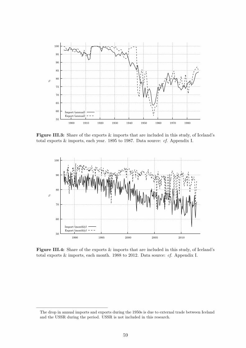
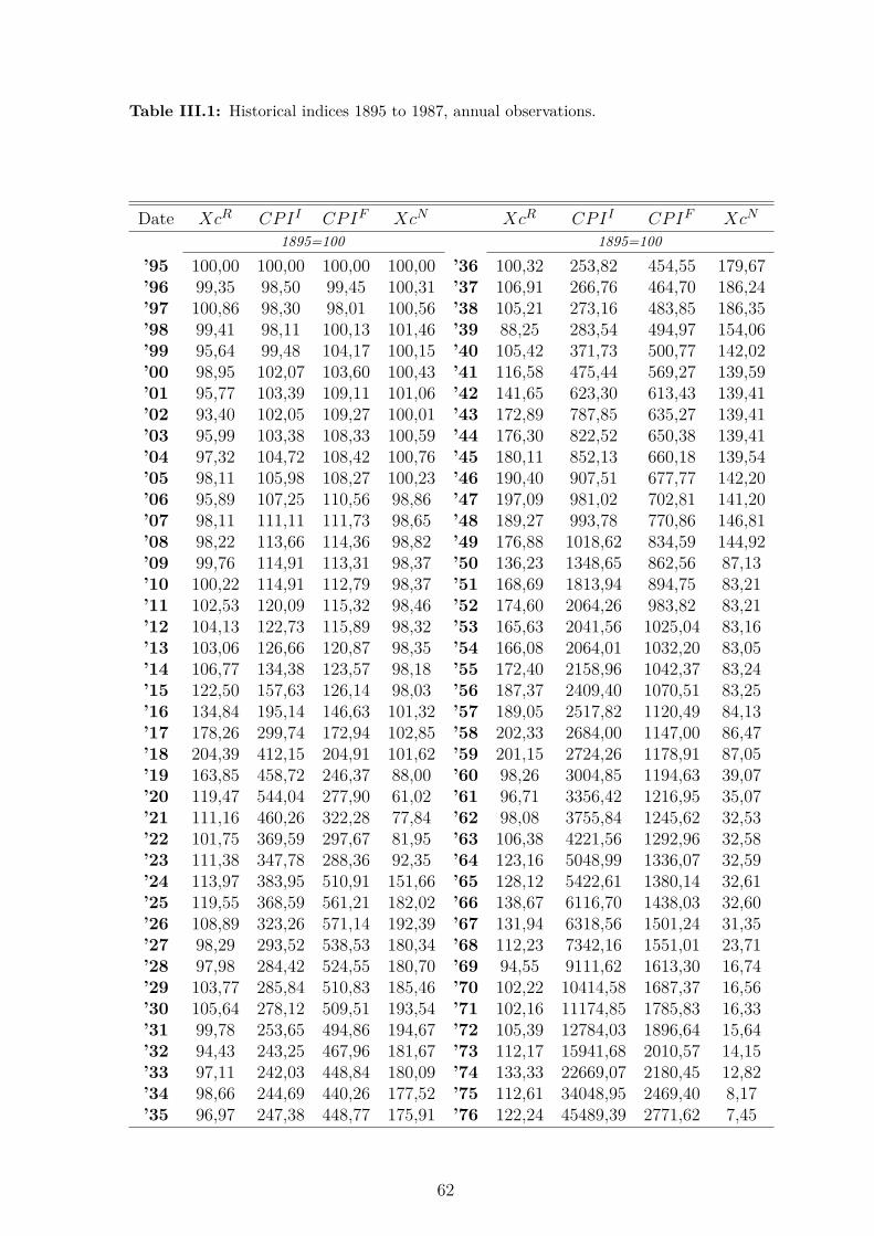
III.4 Share of the exports & imports that are included in this study, ofIceland’s total exports & imports, each month. 1988 to 2012. Datasource: cf. Appendix I. . . . . . . . . . . . . . . . . . . . . . . . . . . 59
III.5 Comparison of the new real effective exchange rate of the Icelandickróna (XcR) & the official real exchange rate of The Central Bank,monthly frequency: 1988 to 2012 (Jan 1988 = 100). Data source: cf.Appendix I & calculations in Section 3. . . . . . . . . . . . . . . . . . 60
III.6 The new nominal effective króna exchange rate (XcN ) and Relativeprices (RelCPI), monthly frequency: 1988 to 2012 (Jan 1988 = 100).Data source: cf. Appendix I & calculations in Section 3. . . . . . . . 60
viii
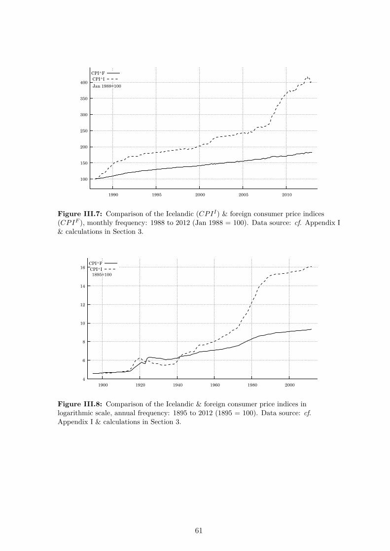
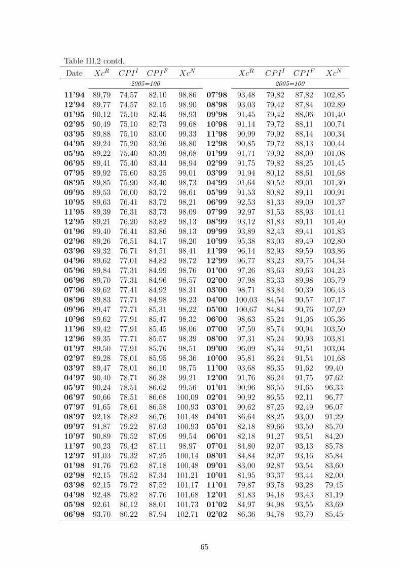
III.7 Comparison of the Icelandic (CPII) & foreign consumer price indices(CPIF ), monthly frequency: 1988 to 2012 (Jan 1988 = 100). Datasource: cf. Appendix I & calculations in Section 3. . . . . . . . . . . 61
III.8 Comparison of the Icelandic & foreign consumer price indices in log-arithmic scale, annual frequency: 1895 to 2012 (1895 = 100). Datasource: cf. Appendix I & calculations in Section 3. . . . . . . . . . . 61
ix
List of Tables
5.1 Unit-root test results for the period 1895-2012, annual data. . . . . . 175.2 Single-equation cointegration test result for the period 1895-2012, an-
nual data. . . . . . . . . . . . . . . . . . . . . . . . . . . . . . . . . . 185.3 Unit-root test results for the period 1895-1960, annual data. . . . . . 235.4 Single-equation cointegration test result for the period 1895-1960, an-
nual data. . . . . . . . . . . . . . . . . . . . . . . . . . . . . . . . . . 245.5 Unit-root test results for the period 1960-2012, annual data. . . . . . 265.6 Single-equation cointegration test result for the period 1960-2012, an-
nual data. . . . . . . . . . . . . . . . . . . . . . . . . . . . . . . . . . 275.7 Unit-root test results for the period 1988-2012, monthly data. . . . . 295.8 Single-equation cointegration test result for the period 1988-2012, monthly
In the modern world, currency exchange rate developments are a fundamental partof international economics. Exchange rates can have a substantial effect on externaltrade and other financial transactions between countries. The more dependent acountry is on external trade, the more currency fluctuations can affect its economy.
Unpredictable exchange rate volatility can sometimes have adverse effects on fin-ancial stability. The fluctuating exchange rate of the Icelandic króna have played amajor role in the history of the Icelandic economy. Iceland is a small, open economythat relies on external trade, with exports and imports averaging around 30 per centof GDP during the past century, cf. Appendix III, Figure 1.
The aim of this study is to examine whether the ISK’s fluctuating exchange rateexhibits a tendency towards mean-reversion; i.e, to determine whether an equilibriumreal exchange rate exists for the ISK in the long run.
Long-run trade-weighted nominal and real effective exchange rate indices are con-structed for the ISK from 1895 to 2012, or almost from its introduction as a currency1.Annual data are used for the period between 1895 and 1988 for the construction ofthe indices. For the period from 1988 to 2012 monthly data are used. The historicalexchange rates are constructed as geometrically weighted chain indices with currenttrade weights based on Iceland’s foreign trade in goods. The consumer price index(CPI) is used for deflation. Annual data are based on 13 of Iceland’s largest tradingpartners, which accounted for at least 70 per cent of Iceland’s total foreign trade ingoods each year, during the period. For the monthly data, two more countries areadded to the dataset, for a total of 15 trading partners which accounted for at least64 per cent of Iceland’s total foreign trade in goods each month, during the period.
Empirical estimations are applied to the new time series. Unit-root and single-equation cointegration tests are performed for stationarity estimation. The meanreversion from PPP deviation is analysed via autoregressive models, with half-lifecalculations based on ordinary least squares (OLS) parameter estimates. Empiricalestimations are applied to the period as a whole, as well as individual estimations fortwo sub-periods, that emerged after a structural-break estimation revealed a break-point at 1960. Separate estimations are also carried out for the post-1988 period,using monthly data.
The results are consistent with similar PPP studies. Evidence supporting relative
1 The first 10 years, between 1885 and 1895, could not be included due to data shortage.
1
PPP convergence is found for all but one of the periods (post-1988), where unit-rootand cointegration test results contradict, indicating a failure of PPP convergence.Half-life estimates are around four years for the period as a whole. The most rapidmean reversion appears during the inter-war and post-1981 periods. The inter-warperiod also shows the least amount of volatility in the real exchange rate of the ISK.
The paper is structured as follows: Section 2 contains a brief overview of thepurchasing power parity theory. Description of the data set and methodology for thecalculations of the historical indices are found in Section 3. Section 4 contains anoverview of the empirical methodology for PPP estimations, followed by empiricalfindings in Section 5. The final section contains the conclusions and a brief discussionof the scope for further research2.
2 Detailed data descriptions, figures, tables, and regression outputs are included in accompanyingappendices.
2
2 Purchasing Power Parity (PPP)
Purchasing power parity (PPP) is one of the fundamental theories in internationaleconomics. The theory postulates that currency exchange rates adjust over time tooffset divergent movements in national price levels. Persistence of real exchange ratescan be used for validation of the purchasing power parity theory, e.g. by estimationof the real exchange rate mean-reversion behaviour. Despite its simplicity, the theoryis widely debated in the literature. The general consensus seems to be that the theoryholds in the long run, although short-run parity convergence is generally not accepted(Kulkarni, 1990-1991).
2.1 Law of One Price
Although the term purchasing power parity was originally coined by Gustav Casselin 1922, the idea behind the theory has been around for much longer and exists todayin a number of variations. The Big Mac index, published by The Economist, is anexample of a well-known variation of PPP. It shares the same fundamental premise asPPP, the so-called law of one price (LOOP). According to LOOP, due to arbitrage,any price difference in an internationally trade-able good between countries shouldnot exist, at least not in the long run. The cheaper good would simply be exportedand transported to the more expensive location until equilibrium in price and quantitywas reached between the two locations3. LOOP is given by:
pt(i) = p∗t (i) +vt
vt = pt(i)−p∗t (i)
pt(i)−vt = p∗t (i)
where pt(i) is the log of the time-t domestic-currency price of good i, p∗(i) is theanalogous foreign-currency price, and vt is the log of the time-t domestic-currencyprice of foreign exchange.
3 Internationally integrated and open markets are necessary for LOOP to hold.
3
2.2 Absolute PPP
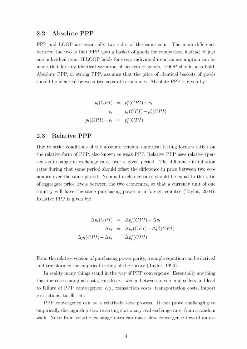
PPP and LOOP are essentially two sides of the same coin. The main differencebetween the two is that PPP uses a basket of goods for comparison instead of justone individual item. If LOOP holds for every individual item, an assumption can bemade that for any identical variation of baskets of goods, LOOP should also hold.Absolute PPP, or strong PPP, assumes that the price of identical baskets of goodsshould be identical between two separate economies. Absolute PPP is given by:
pt(CPI) = p∗t (CPI) +vt
vt = pt(CPI)−p∗t (CPI)
pt(CPI)−vt = p∗t (CPI)
2.3 Relative PPP
Due to strict conditions of the absolute version, empirical testing focuses rather onthe relative form of PPP, also known as weak PPP. Relative PPP uses relative (per-centage) change in exchange rates over a given period. The difference in inflationrates during that same period should offset the difference in price between two eco-nomies over the same period. Nominal exchange rates should be equal to the ratioof aggregate price levels between the two economies, so that a currency unit of onecountry will have the same purchasing power in a foreign country (Taylor, 2004).Relative PPP is given by:
From the relative version of purchasing power parity, a simple equation can be derivedand transformed for empirical testing of the theory (Taylor, 1996).
In reality many things stand in the way of PPP convergence. Essentially anythingthat increases marginal costs, can drive a wedge between buyers and sellers and leadto failure of PPP convergence; e.g., transaction costs, transportation costs, importrestrictions, tariffs, etc.
PPP convergence can be a relatively slow process. It can prove challenging toempirically distinguish a slow reverting stationary real exchange rate, from a randomwalk. Noise from volatile exchange rates can mask slow convergence toward an ex-
4
isting equilibrium. Estimating longer time series that incorporate different exchangerate policies, e.g. combining fixed and floating exchange rate periods in one con-tinuous series can increase the accuracy of empirical testing. Using a multi-countryenvironment for estimation is also important for increased accuracy.
A drawback of the purchasing power parity theory is the assumption that tradingrelations are the sole contributing factor to price and exchange rate developments.This is an understatement as many other factors influence exchange rate dynam-ics. The interest rate spread is thought to be one of those influencing factors. Theuncovered interest rate parity theory (UIP) relies on the premise that the interestrate difference between two financial assets should be offset by the expected rateof change in the exchange rate between two currencies over the period to maturity(Beirne, 2010).
A wealth of literature concerning deviations from purchasing power parity exists.Rogoff (1996) writes about the reluctance of real exchange rate mean-reversion whenestimated4. He points out that storage costs, labour costs, transportation costs, tariffsand non-tradable components of tradable goods, drive a wedge between domestic andforeign prices.
The Balassa-Samuelson effect, one of the driving factors of real currency exchangerates, could be an underestimated culprit behind the failure of PPP convergence5.Government spending could also be a contributing factor, leading to PPP failure, asthe non-tradable sector is usually more influenced by government spending than thetradable sector.
Possible methodology errors in PPP estimation might lead to non-stationary andslow mean-reversion estimations. Temporal aggregation and linear specification areunderestimated factors contributing to slow mean reversion estimates of real exchangerates, according to Taylor (2000). Linear restrictions force shocks to adjust back in alinear fashion, and therefore cannot account for mean reversion adjustments, which,might damp out at a faster rate than it began. Half-life estimation using aggregateddata, whether of annual, quarterly or monthly frequency, usually overestimates half-life times, because high-frequency adjustment processes can never be evaluated bylow-frequency data; the greater the aggregation, the greater the bias. Combining thetwo errors can exacerbate the problem even further.
Finally, the speed of reversion to parity is likely to depend on goods-specific
4 Rogoff’s (1996) purchasing power parity puzzle is as follows: “How can one reconcile the enormousshort-term volatility of real exchange rates with the extremely slow rate at which shocks appear todamp out?”.
5 The Balassa-Samuelsson effect states that measured in the same unit, price levels in high incomecountries are higher than those in low income countries, due to differences in productivity in thetradable and non-tradable sectors. The non-tradable sector is more affected than the tradablesector, consequently the Balassa-Samuelsson effect is more pronounced in the CPI than WPI(Rogoff, 1996).
5
characteristics, and is therefore not homogeneous across sectors. Failure to accountfor cross-sectoral heterogeneity in the dynamic properties of the typical price indexcomponents affects the estimated half-lives (Imbs et al., 2002).
6
3 Historical ISK Exchange Rate
The Central Bank of Iceland is responsible for official exchange rate calculationsfor the ISK. The bank bases calculations of the nominal exchange rate on predeter-mined weights. The composition of Iceland’s external trade from the previous yeardetermines weight composition. Nominal exchange rate movements reflect appre-ciation/depreciation vis-à-vis the currencies of the major trading nations that areincluded in the calculations.
Two separate real exchange rates for the króna are published by the Central Bank.One is based on relative consumer prices and the other is based on relative unit labourcosts. An increase in the real exchange rate describes a real appreciation of the ISKrelative to its trading partners. Real exchange rates are essentially indicators ofdevelopments in a country’s international competitiveness (Central Bank of Iceland,2013).
Annual real exchange rates for the ISK are available from the Central bank dat-ing back to 1980. Monthly data are available from 1985. No official real exchangerate data are available prior to 1980. In an article published in 1985 the real ISKexchange rate is calculated back to 1914 (Nordal & Tómasson, 1985). Calculationswere based on data from three of Iceland‘s largest trading partners: the US, the UK,and Denmark. No real exchange rate data for the ISK are available for the periodbefore 1914.
To construct historical time-series for PPP analysis, a multi-country environmentis needed in order to reflect changes in trade patterns on a current basis. Using datafrom two countries for estimation, is unlikely to yield an adequate explanation ofexchange rate behaviour that is driven by interactions of multiple trading partners(Beirne, 2010).
3.1 The Data Set
For historical exchange rate calculations, annual external trade data for Iceland werecompiled for 13 of Iceland’s largest trading partners during the period from 1895 to1988. The trading partners are Denmark, Finland, France, Germany, Italy, Japan,the Netherlands, Norway, Portugal, Spain, Sweden, the UK, and the US. Duringthe period, these countries accounted for at least 70 per cent of total foreign trade
7
and an average of 87 per cent6. Monthly data were compiled from January 1988through December 2012. In addition to the previous list of trading partners, twomore countries are added for the monthly data: Belgium and Switzerland. In all,these countries accounted for at least 64 per cent of Iceland’s total external trade,with an average of 83 per cent7.
Annual averages of consumer price indices were compiled for the previously listedcountries, for the period from 1895 to 1988. Monthly averages were compiled from1988 through 2012. When available, the consumer price index is replaced by theHarmonized index of consumer prices (HICP)8.
Annual averages of bilateral exchange rates of the Icelandic króna versus thecurrencies of the previously listed countries were compiled for the period from 1895to 1988. Monthly averages were used for the period between 1988 and 2012. Furtherdata details can be found in the appendices.
The following time-series were constructed:
1. XcN : Nominal effective exchange króna rate. Annual observations from1895 to 1988. Monthly observations from 1988m01 through 2012m12. Anincrease in the nominal index represents an appreciation of the ISK’s nominalvalue versus the currencies of Iceland’s main trading partners.
2. XcR: Real effective exchange króna rate. Annual observations from 1895to 1988. Monthly observations from 1988m01 through 2012m12. An increasein the real index represents an appreciation of the ISK’s real value versus thecurrencies of Iceland’s main trading partners.
3. CPII : Consumer price index for Iceland. Annual observations from 1895to 1988. Monthly observations from 1988m01 through 2012m12.
4. CPIF : Foreign consumer price index. Annual observations from 1895 to1988 and monthly observations from 1988m01 through 2012m12. The index isconstructed as geometrically weighted average of Iceland’s trading partners.
The consumer price index (CPI), wholesale price index (WPI) and producer priceindex (PPI) are all commonly used as deflators for PPP estimation. The structure ofthese price indices can vary across countries, especially in older data (Froot & Rogoff,1994). Different index structure can distort comparison, causing biased convergenceestimations. Other factors including different preferences, traditions, and others, canalso affect the index structure in each country, reducing reliability for comparison9.6 With an exception during the 1950s, cf. Appendix III.7 Cf. Appendix III, Figures 3 & 4.8 Initial starting dates of HICP measurements, vary from country to country.9 HICP should eliminate this distortion. cf. Appendix I, for details.
8
The use of WPI or PPI seem to give more accurate results when it comes to PPP es-timations. They usually place greater emphasis on tradable goods than the consumerprice index, which ordinarily includes substantial amounts of non-tradable goods, aswell as being generally more susceptible to effects caused by indirect taxes and sub-sides (Taylor & Taylor, 2004). Nonetheless, the consumer price index can serve as agood substitute for the WPI and PPI10.
3.2 Nominal Effective Exchange Rate Index
In order to calculate the historical real exchange rate for the ISK, historical nominalexchange rates must be constructed first. The nominal exchange rate index is cal-culated as a geometrically weighted chain index with current weights based on tradestatistics for each period since 1895. The index is based on Iceland’s total foreigntrade in goods11. The weights used for calculating the index are based on the sumof total bilateral imports and exports of goods vis-à-vis the major trading partnersthat are included in this study.
The historical nominal effective króna rate index (XcN ) is calculated as a geomet-rically weighted chain index with current weights based on trade statistics for eachperiod. The relative change in the XcN index is given by:
XcNtXcNt−1
=n∏t=1
(BEitBEit−1
)wit−1
wheren∑i=1
wit−1 = 1
where BEit is the bilateral exchange rate between the Icelandic króna and currencyi in period t (amount of foreign currency i per Icelandic króna). The index is ageometrically weighted chain where wit−1 represents the weight for currency i fromperiod t−1 to period t. The weight is structured as follows:
wit−1 =
(IP it−1 +XP it−1
)(∑IP t−1 +∑
XP t−1)
wit−1 is based on the sum of the Icelandic bilateral imports and exports of goodsin period t− 1 vis-à-vis country i relative to total Icelandic imports and exports ofgoods vis-à-vis the previously listed countries. Changes in the currencies from 1895to 1896 are thus weighted with trade weights reflecting the trade pattern in year 1895etc. An increase in the XcN describes an overall appreciation of the króna vis-à-visthe currencies of the major trading partners (Abildgren, 2004).
10The consumer price index is the only available deflator for Iceland, covering such a long period.11Data aggregated, i.e. no category distinction.
9
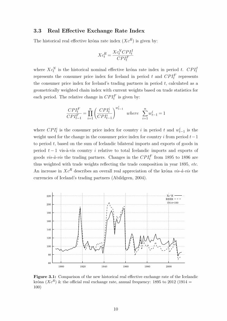
3.3 Real Effective Exchange Rate Index
The historical real effective króna rate index (XcR) is given by:
XcRt = XcNt CPIIt
CPIFt
where XcNt is the historical nominal effective króna rate index in period t. CPIIt
represents the consumer price index for Iceland in period t and CPIFt representsthe consumer price index for Iceland’s trading partners in period t, calculated as ageometrically weighted chain index with current weights based on trade statistics foreach period. The relative change in CPIFt is given by:
CPIFtCPIFt−1
=n∏i=1
(CPIitCPIit−1
)wit−1
wheren∑i=1
wit−1 = 1
where CPIit is the consumer price index for country i in period t and wit−1 is theweight used for the change in the consumer price index for country i from period t−1to period t, based on the sum of Icelandic bilateral imports and exports of goods inperiod t− 1 vis-à-vis country i relative to total Icelandic imports and exports ofgoods vis-à-vis the trading partners. Changes in the CPIFt from 1895 to 1896 arethus weighted with trade weights reflecting the trade composition in year 1895, etc.An increase in XcR describes an overall real appreciation of the króna vis-à-vis thecurrencies of Iceland’s trading partners (Abildgren, 2004).
60
80
100
120
140
160
180
200
220
1900 1920 1940 1960 1980 2000
Xc^RREER1914=100
Figure 3.1: Comparison of the new historical real effective exchange rate of the Icelandickróna (XcR) & the official real exchange rate, annual frequency: 1895 to 2012 (1914 =100)
10
Appreciation of the real exchange rate usually suggests that the country is growingwealthier, with increased competitiveness. This generally applies to foreign trade.Increased efficiency and competitiveness in non-exportable domestic services usuallycarries no weight in the fluctuations of a country’s currency exchange rate (Froot &Rogoff, 1994).
Comparison of the developments between the new historical real effective exchangerate (XcR) and official data can be seen in Figure 3.112. Figure 3.2 shows the de-velopment of the new historical nominal effective exchange rate (XcN ) and relativeprices (RelCPI) for the period, in logarithmic scale13.
0
50
100
150
200
1900 1920 1940 1960 1980 2000
Xc^NRelCPI
1895=100
Figure 3.2: Historical nominal effective exchange rate of the Icelandic króna (XcN ) &relative prices (RelCPI= (CPIF
t /CPIIt )) in logarithmic scale, annual frequency: 1895 to
2012 (1895 = 100)
12In order to make one continuous time-series covering the whole period, annual averages are cal-culated from monthly data post-1988.
13For more figures, cf. Appendix III.
11
4 Econometric Methodology
4.1 Stationarity
The mean reverting behaviour of the real exchange rate is commonly estimated viaunit-root and cointegration testing procedures. The basic idea is to test whether theXcR behaves like a random walk, where a variable’s value equals its previous valuewith a stochastic term added. In such a case the time series is said to contain a unitroot, i.e. it is non-stationary14.
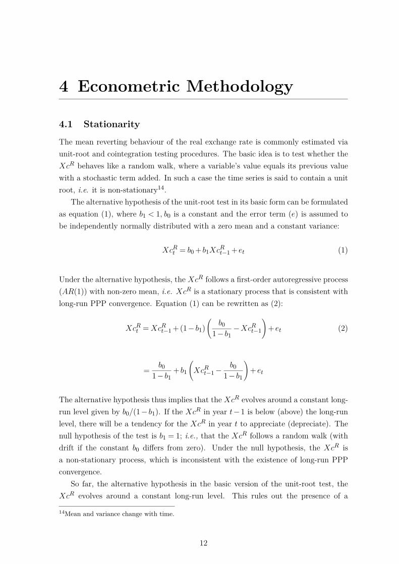
The alternative hypothesis of the unit-root test in its basic form can be formulatedas equation (1), where b1 < 1, b0 is a constant and the error term (e) is assumed tobe independently normally distributed with a zero mean and a constant variance:
XcRt = b0 + b1XcRt−1 + et (1)
Under the alternative hypothesis, the XcR follows a first-order autoregressive process(AR(1)) with non-zero mean, i.e. XcR is a stationary process that is consistent withlong-run PPP convergence. Equation (1) can be rewritten as (2):
XcRt =XcRt−1 + (1− b1)(
b01− b1
−XcRt−1
)+ et (2)
= b01− b1
+ b1
(XcRt−1−
b01− b1
)+ et
The alternative hypothesis thus implies that the XcR evolves around a constant long-run level given by b0/(1− b1). If the XcR in year t−1 is below (above) the long-runlevel, there will be a tendency for the XcR in year t to appreciate (depreciate). Thenull hypothesis of the test is b1 = 1; i.e., that the XcR follows a random walk (withdrift if the constant b0 differs from zero). Under the null hypothesis, the XcR isa non-stationary process, which is inconsistent with the existence of long-run PPPconvergence.
So far, the alternative hypothesis in the basic version of the unit-root test, theXcR evolves around a constant long-run level. This rules out the presence of a
14Mean and variance change with time.
12
deterministic trend in the real effective exchange rate. Unit-root presence can leadto spurious correlation in regression analysis which causes parameter estimation foradjusted R2 and t-scores to be overestimated. A trend-stationary variable is subjectto non-stationary estimation, if the trend is not accounted for. Adding a time trendparameter to the model, can prevent spurious regression. A deterministic trend couldbe formalised in a unit-root test where the alternative hypothesis in its basic versionis given by equation (3):
XcRt = b0 + b1XcRt−1 +dt+ et (3)
This alternative hypothesis, where b1 < 1, thus implies that the XcR evolves arounda deterministic time trend (i.e. a trend-stationary process). The forces of the relativePPP ensure a long-run mean reversion towards the trend. The null hypothesis of thetest is b1 = 1, i.e. that the XcR follows a random walk (with drift if the constantb0 6= 0) around a deterministic trend (Abildgren, 2004).
4.1.1 Unit-root: Augmented Dickey Fuller
The ADF test has become the “standard” test for stationarity in the literature.However, it should be noted that the power of the ADF test is not very strong.It can therefore be difficult to reject the null hypothesis of non-stationarity evenwhen it is false, especially if the stationary alternative has a sum of autoregressiveparameters (∑bj) close to one (i.e. in cases where convergence towards PPP is slow).
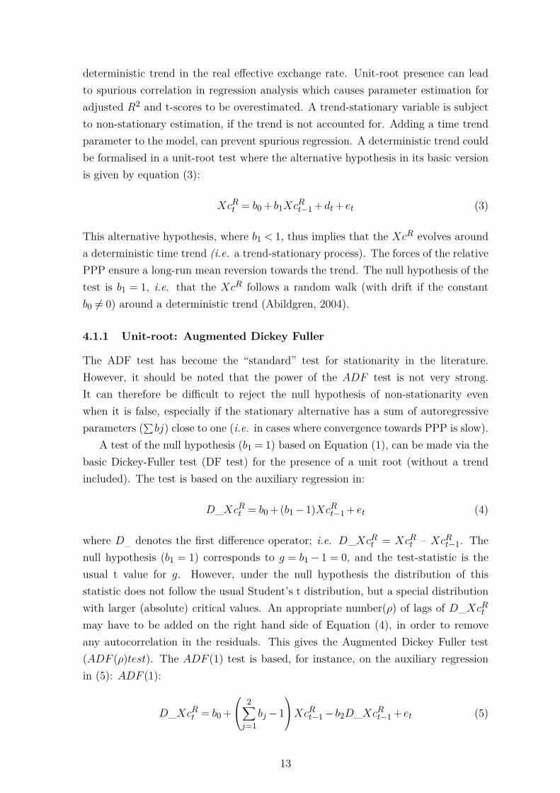
A test of the null hypothesis (b1 = 1) based on Equation (1), can be made via thebasic Dickey-Fuller test (DF test) for the presence of a unit root (without a trendincluded). The test is based on the auxiliary regression in:
D_XcRt = b0 + (b1−1)XcRt−1 + et (4)
where D_ denotes the first difference operator; i.e. D_XcRt = XcRt – XcRt−1. Thenull hypothesis (b1 = 1) corresponds to g = b1− 1 = 0, and the test-statistic is theusual t value for g. However, under the null hypothesis the distribution of thisstatistic does not follow the usual Student’s t distribution, but a special distributionwith larger (absolute) critical values. An appropriate number(ρ) of lags of D_XcRtmay have to be added on the right hand side of Equation (4), in order to removeany autocorrelation in the residuals. This gives the Augmented Dickey Fuller test(ADF (ρ)test). The ADF (1) test is based, for instance, on the auxiliary regressionin (5): ADF (1):
D_XcRt = b0 + 2∑j=1
bj−1XcRt−1− b2D_XcRt−1 + et (5)
13
and ADF (ρ) is based on:
D_XcRt = b0 +ρ+1∑j=1
bj−1XcRt−1 +
ρ∑j=1
b∗jD_XcRt−j + et (6)
where b∗j are functions of b2, ..., bp+1. The null hypothesis of non-stationarity of theADF (ρ) test is that g =∑
bj−1 = 0 and the test-statistic is the usual t value for g.However, as it was the case in the DF-test, the distribution of this statistic is non-standard. With no significant lags, the ADF (0) test is identical to the DF test. Withρ significant lags in an ADF (ρ) test, the XcR follows an (ρ+1)-order autoregressivepath under the alternative hypothesis(∑bj < 1)15:
XcRt = b0 +ρ+1∑j=1
bjXcRt−j + et (7)
(7) can be rewritten as (8):
XcRt = b0
1−∑ρ+1j=1 bj
+ρ+1∑j=1
bjXcRt−j− b0
1−∑ρ+1j=1 bj
+ et (8)
The alternative hypothesis thus implies that the XcR evolves around a constantlong-run level given by b0/(1−
After unit-root testing, determining order of integration is the next logical step indetermining whether the variables share a similar stochastic trend; that is, discoveringwhether cointegration relationships exist between them. Consider again the simplefirst-order autoregressive model in Equation (1). If XcRt follows a random walk, thenb1 = 0. If the error term et is stationary, i.e., does not follow a random walk then thefirst difference D_XcRt =XcRt −XcRt−1 is also stationary:
XcRt = b0 + b1XcRt−1 + et
D_XcRt = XcRt −XcRt−1 = et
The cointegration test is essentially a stationarity test of the residuals. (Griffithset al., 2008). Cointegration entails that the error terms et are stationary, whichmeans that they never diverge too far from each other. Cointegration holds that the
15The number of lags in the ADF test, has been chosen so that autocorrelation is minimized in theresiduals from the auxiliary regression.
14
combination of two or more non-stationary series can yield a long-run relationship aslong as the series are integrated of the same order, non-stationarity can therefore becancelled out, and a stationary relationship observed instead (Beirne, 2010).
Cointegration consists of matching the degree of non-stationarity of the variablesin an equation in a way that makes the error term and residuals of the equationstationary and rids the equation of any spurious regression estimation (Studenmund,2011).
The Engle-Granger single-equation cointegration test is an alternative way to theunit-root for relative PPP assessment. Should relative PPP hold, the real effectivekróna rate must be equal to a constant (K):
XcR = XcNCPIItCPIFt
= XcNt(CPIFt /CPIIt )
= XcNtRelCPIt
=K (9)
Where XcN is the nominal effective króna rate and RelCPI = (CPIFt /CPIIt ) is theratio between the domestic and foreign price indices. Adding an error term (e) whichis assumed to be independently normally distributed with a zero mean and constantvariance, (9) becomes:
ln(XcNt )− ln(RelCPIt) = ln(K) + et (10)
If ln(XcNt ) and ln(RelCPIt) are both integrated of first order (I(1)), they arecointegrated if the natural logarithm of the real effective króna rate is stationary(ln(XcRt ) = ln(XcNt )− ln(RelCPIt)). This can be evaluated via ADF tests onln(XcNt ), ln(RelCPIt) and ln(XcRt ). If ln(XcNt ) and ln(RelCPIt) are I(1) andln(XcRt ) is stationary, the results support a hypothesis of long-run relative PPP con-vergence, and the cointegrating relationship implied by equation (10) can be viewedas the long-term relationship between ln(XcNt ) and ln(RelCPIt). If ln(XcNt ) andln(RelCPIt) are both stationary, then the ln(XcRt ) is also stationary. This also givessupport for long-run relative PPP. If stationarity of ln(XcRt ) is rejected, there is nosupport for relative PPP (Abildgren, 2004).
4.2 Mean-Reversion
4.2.1 Half-Life Estimation
The validity of long-run PPP depends not just on the absence of a unit-root intime series. A sufficient degree of mean-reversion in the real exchange rate is alsoimportant if PPP assumption-based models are to have real-world meaning (Cashin& McDermott, 2003).
In a first-order autoregressive process (AR(1)) such as Equation (2), parameter
15
b1 determines the speed of mean reversion, since (1− b1) per cent of the absolutedeviation from the long-run level is expected to close each year. The number of yearsbefore one-half of a deviation from the long-run level of the real effective exchangerate is extinguished, the so-called Half-life (HL) can be found as:
HLin(1) = ln(0.5)ln(b1) (11)
where ln denotes the natural logarithmic function. For an AR(ρ) process, a commonlyused approximate formula for the number of years before one-half of a shock to thereal effective exchange rate is extinguished when estimating is given by:
HLin(6) = ln(0,5)ln(∑p+1
j=1 bj) (12)
Ordinary least squares (OLS) estimates of the parameters to the lagged dependentvariables in Equations (1), and (6) will be downward biased in finite even when theXcR is stationary. In a linear framework, half-lives can only be considered as a simple“summary measure” of mean reversion, as speed of adjustment may not always beuniform (Abildgren, 2004)16.
4.2.2 Bias-Adjusted Half-Life Estimation
More accurate estimations for half-life analysis in a linear autoregressive frameworkmight be achieved through bias adjusted estimation. A downward bias in the para-meters implies that point estimates for half-lives will be too low when calculatedfrom OLS estimates (Abildgren, 2004). In the case of the AR(1)-model for XcR,a bias-adjusted half-life may be calculated from the OLS estimate as bias-adjustedOLS estimate for half-life in AR(1) model for XcR:
ln(0,5)ln(b1NN−3 + 1
N−3
)
where N denotes the number of observations. In the case of an AR(2)-model for theXcR, a bias-adjusted approximate half-life may be calculated from the OLS estimatesas the bias-adjusted OLS estimate for half-life in AR(2) model for XcR.
ln(0,5)ln(b1NN−1 + 1
N−1 +(
1N−1 + 1
)(b2NN−4 + 2
N−4
))
16A time trend parameter, is usually not included in half-life estimation, as it is not consistent withthe idea of mean reversion (Cashin & McDermott, 2003).
16
5 Empirical Findings
5.1 1895 to 2012
5.1.1 Unit-Root
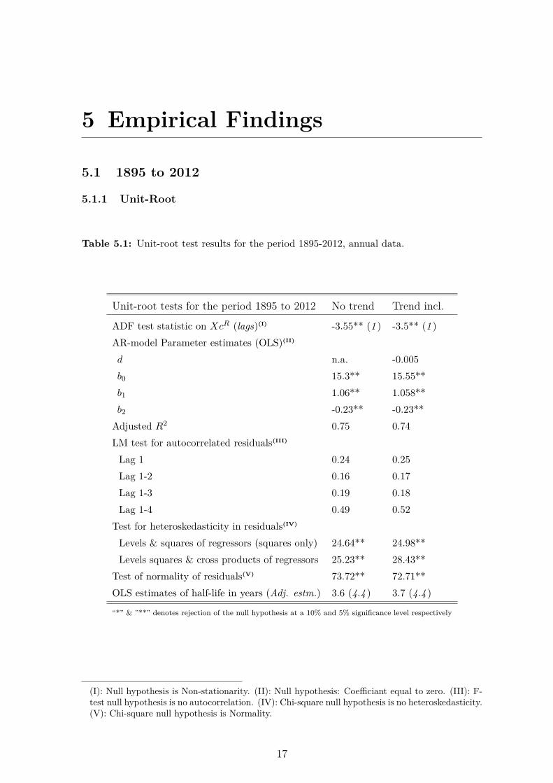
Table 5.1: Unit-root test results for the period 1895-2012, annual data.
Unit-root tests for the period 1895 to 2012 No trend Trend incl.
ADF test statistic on XcR (lags)(I) -3.55** (1 ) -3.5** (1 )AR-model Parameter estimates (OLS)(II)
d n.a. -0.005b0 15.3** 15.55**b1 1.06** 1.058**b2 -0.23** -0.23**
Adjusted R2 0.75 0.74LM test for autocorrelated residuals(III)
Levels & squares of regressors (squares only) 24.64** 24.98**Levels squares & cross products of regressors 25.23** 28.43**
Test of normality of residuals(V) 73.72** 72.71**OLS estimates of half-life in years (Adj. estm.) 3.6 (4.4 ) 3.7 (4.4 )
“*” & ”**” denotes rejection of the null hypothesis at a 10% and 5% significance level respectively
(I): Null hypothesis is Non-stationarity. (II): Null hypothesis: Coefficiant equal to zero. (III): F-test null hypothesis is no autocorrelation. (IV): Chi-square null hypothesis is no heteroskedasticity.(V): Chi-square null hypothesis is Normality.
17
Estimation results for the period as a whole support long-run relative purchasingpower parity convergence. The null hypothesis of non-stationarity is rejected at a 5per cent significance level, both with and without a trend parameter present. Estim-ations show no trace of autocorrelation in the residuals; however, heteroskedasticityand non-normality of the residuals are evident. The underlying univariate autore-gressive models explain around 75 per cent of the linear variation in the real effectiveexchange rate for the period.
Although insignificant, the negative sign for the trend parameter could indicate aslow decline in Iceland’s competitiveness relative to its major trading partners overthe period. Another possible explanation could be due to biased parameter estimates,caused by an unknown structural-break in the series.
5.1.2 Cointegration
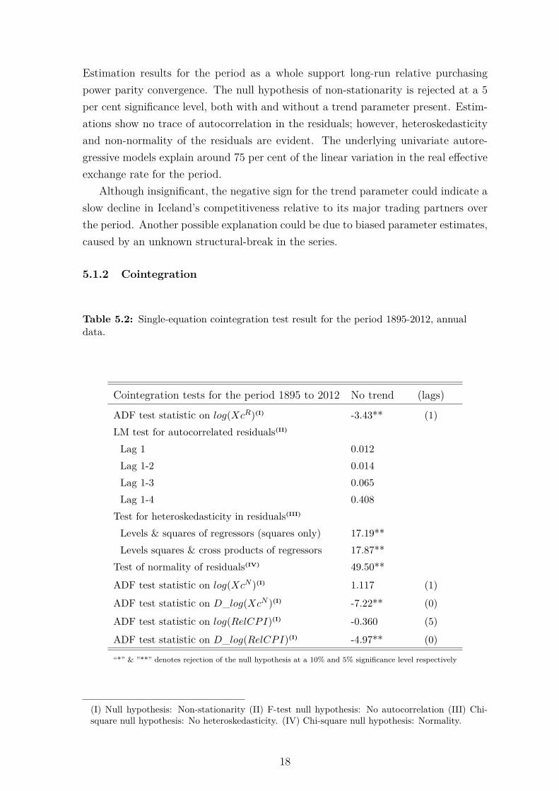
Table 5.2: Single-equation cointegration test result for the period 1895-2012, annualdata.
Cointegration tests for the period 1895 to 2012 No trend (lags)
ADF test statistic on log(XcR)(I) -3.43** (1)LM test for autocorrelated residuals(II)
Lag 1 0.012Lag 1-2 0.014Lag 1-3 0.065Lag 1-4 0.408
Test for heteroskedasticity in residuals(III)
Levels & squares of regressors (squares only) 17.19**Levels squares & cross products of regressors 17.87**
Test of normality of residuals(IV) 49.50**
ADF test statistic on log(XcN )(I) 1.117 (1)
ADF test statistic on D_log(XcN )(I) -7.22** (0)
ADF test statistic on log(RelCPI)(I) -0.360 (5)
ADF test statistic on D_log(RelCPI)(I) -4.97** (0)
“*” & ”**” denotes rejection of the null hypothesis at a 10% and 5% significance level respectively
(I) Null hypothesis: Non-stationarity (II) F-test null hypothesis: No autocorrelation (III) Chi-square null hypothesis: No heteroskedasticity. (IV) Chi-square null hypothesis: Normality.
18
OLS half-life estimates for the period are around 3.6 years, and around 4.4 years whenadjusted for bias17. Results from single-equation cointegration tests confirm previousresults of stationarity. Unit-root presence is rejected in log(XcR) at a 5 per centsignificance level. Although unit-root presence in log(XcN ) and log(RelCPI) cannotbe rejected, it is rejected for the first difference of both series which makes themintegrated of first order I(1). Stationarity of log(XcR) also indicates a cointegrationrelationship between log(XcN ) and log(RelCPI).
17Bias-adjusted half-life estimates produce longer half-life times, which is consistent with a prioriexpectations.
19
5.2 Structural Break Estimation
5.2.1 QLR Unknown Breakpoint Estimation
Structural breaks in time-series that are not accounted for, can lead to biased para-meter estimates. They can also lead unit-root tests to falsely accept a null hypothesisof non-stationarity (Byrne & Perman, 2006).
Although visual inspection of time-series can give indication of structural breaks,empirical testing is necessary to determine specific breakpoint dates. The Chow testis commonly used to test for structural breaks. The test essentially splits the sampleinto two sub-periods, evaluates the parameters for each sub-period, and compares theF statistics. The Chow test is given by:
Fn
(m
n
)= Fn(λ) = (SSR1,n− (SSR1,m+SSRm+1,n))/k
(SSR1,m+SSRm+1,n)/(n−2k)
where SSR is the sum of squared residuals. The main disadvantage of using the Chowtest is that it requires a priori knowledge about brake dates. Choosing a breakpointbased on knowledge about the data can lead to true break dates being overlooked.Possible candidates can be endogenous; e.g., correlated with the data, etc.
An alternative approach to the Chow test is Quandt’s LR test with an unknownbreak date, also known as the QLR test (Hansen, 2001). The QLR test does notrequire knowledge about breakpoints beforehand. The QLR test applies a series ofChow tests to all possible breakpoints in the time-series and plots the test statistic.The QLR test is given by:
QLR = maxm∈[m0,m1]
Fn
(m
n
)= maxλ∈[λ0,λ1]
Fn(λ)
λi = mi
n= trimmingparameters, i= 0,1
When testing for unknown break dates, the usual χ2 likelihood distribution is notappropriate. χ2 critical values can lead to breakpoints being estimated as significantwhen they are not. Andrews (1993) provides a table of asymptotic critical valuesthat give a more accurate likelihood distribution, appropriate for the Quandt statisticassessment. These values are considerably larger than χ2 asymptotic critical valuesand therefore less likely to reject a null hypothesis of no structural break18.
18The largest break test-point on the graph is called the Quandt statistic, after Richard E. Quandtwho proposed the test.
20
0
2
4
6
8
10
12
14
16
1920 1930 1940 1950 1960 1970 1980 1990
Chow F-statisticChow F-statistic (trend incl.)
Chi² (3)
Chi² (4)
Andrews (3)
Andrews (4)
Figure 5.1: QLR unknown structural break test for the period 1913 to 1994, w. 15 percent trimming (λ0.15)
In Figure 5.1, estimated Chow statistics have been plotted as a function of breakdates, covering the period from 1913 through 199419. The visible peaks at 1960are the Quandt statistics with the estimated values 40.1 and 49.3 for the solidand dotted line, respectively. Also plotted on the graph are horizontal lines rep-resenting the following asymptotic critical values: χ2
0.95(3) = 7.81, χ20.95(4) = 9.49,
Andrews CV0.9(ρ3, λ0.15) = 12.28 and Andrews CV0.9(ρ4, λ0.15) = 14.3620. Break-points too close to the beginning or end of a sample cannot be considered, as thereare not enough observations to identify the sub-sample parameters (Hansen, 2001).Andrews (1993) recommends 15 per cent trimming (λ0.15) of each end if no priorknowledge of brake-dates exists.
Both critical values for the χ2 likelihood distribution reject the null hypothesisof no structural break at a 5 per cent significance level by a substantial margin.Andrews CV0.9(ρ3, λ0.15) also rejects the null hypothesis of no structural break at a10 per cent significance level. For the period de-trended, structural break presencecannot be rejected at 10 per cent significance level based on AndrewsCV0.9(ρ4, λ0.15).
A CUSUMQ test supports the previous QLR test results, by rejecting variancestability at a 95 per cent confidence level at the same breakpoint, i.e. 1960 (cf. Figure5.2).
Historical interpretations might support a possible structural breakpoint at 1960.During the years leading up to 1960 a complex multiple exchange rate system was inplace. The official ISK exchange rate during the period from 1951 to 1960 was not19The dotted line represents the time period de-trended.20χ2critical values are at a 5 per cent significance level. Andrews critical values are at a 10 per centsignificance level.
21
registered correctly. The period is characterized by heavy import restrictions, tariffs,and strict capital controls (Magnússon, 2012)21.
-0,2
0
0,2
0,4
0,6
0,8
1
1,2
1900 1920 1940 1960 1980 2000 2020
Observation
CUSUMSQ plot with 95% confidence band
Figure 5.2: CUSUMQ parameter stability tests for the period 1895 to 2012.
21A so-called “Boat-currency-system” was put in place to support the marine export sector, mostlyat the expense of the importing sectors.
22
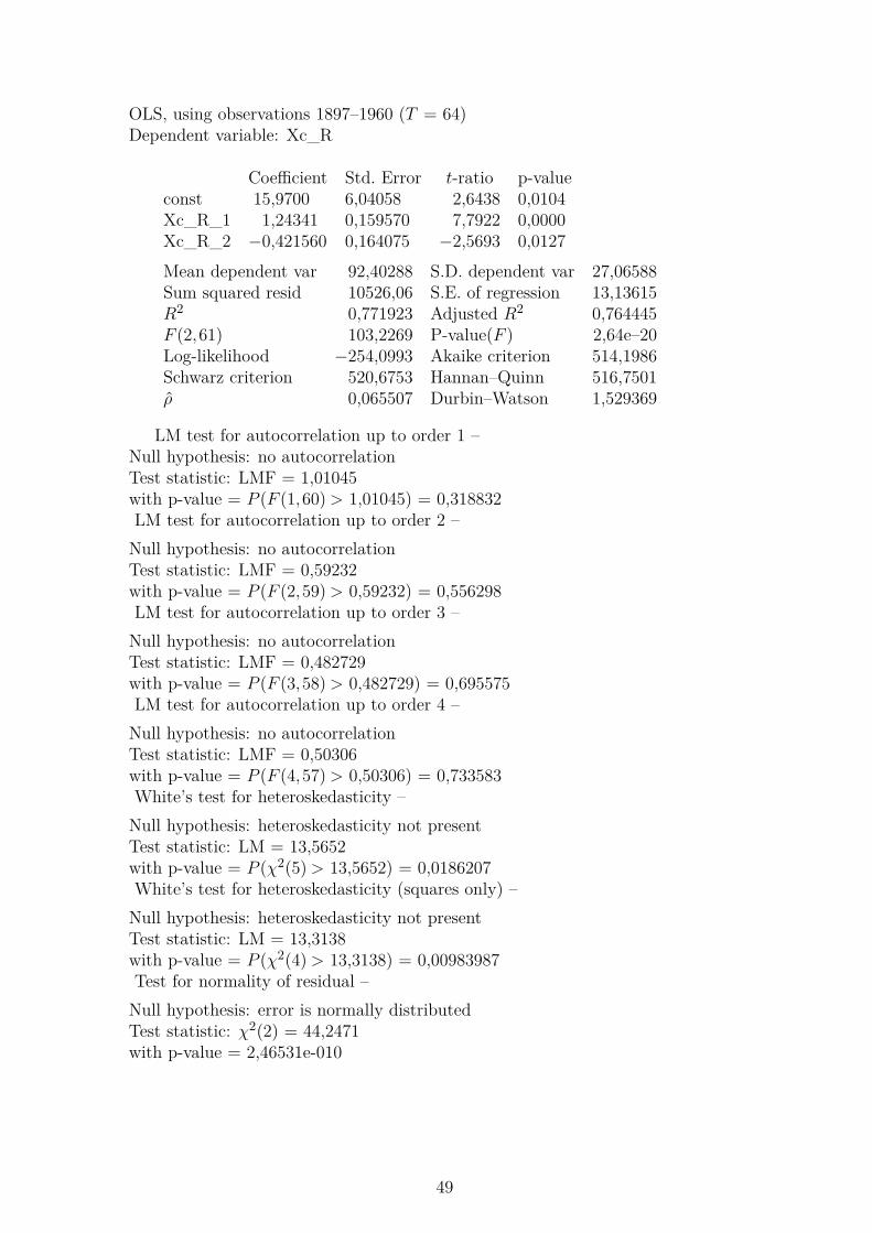
5.3 1895 to 1960
5.3.1 Unit-Root
Table 5.3: Unit-root test results for the period 1895-1960, annual data.
Unit-root tests for the period 1895 to 1960 No trend Trend incl.
ADF test statistic on XcR (lags)(I) -2.81* (1 ) -3.07 (1 )AR-model Parameter estimates (OLS)(II)
d n.a. n.a.b0 15.97** n.a.b1 1.24** n.a.b2 -0.42** n.a.
Adjusted R2 0.76 n.a.LM test for autocorrelated residuals(III)
Levels & squares of regressors (squares only) 13.31** 13.01**Levels squares & cross products of regressors 13.57** 19.68**
Test of normality of residuals(V) 44.25** 44.91**OLS estimates of half-life in years (Adj. estm.) 3.5 (4.7 ) n.a.
“*” & ”**” denotes rejection of the null hypothesis at a 10% and 5% significance level respectively
For the 1895-1960 period, non-stationarity is rejected at a 10 per cent significancelevel without trend22. Estimations show no trace of autocorrelation in the residuals.Heteroskedasticity and non-normality presence in the residuals is not rejected. Theunderlying univariate autoregressive models explain around 76 per cent of the linearvariation in the real exchange rate for the period. Mean-reversion estimation producessimilar results to the half-life estimates for the period as a whole, around 3.5 years,and 4.7 years when adjusted for bias.
(I) Null hypothesis: Non-stationarity (II) Null hypothesis: Coefficiant equal to zero (III) F-testnull hypothesis: No autocorrelation (IV) Chi-square null hypothesis: No heteroskedasticity. (V)Chi-square null hypothesis: Normality.
22For the de-trended period, unit-root presence could not be rejected, parameter estimates weretherefore omitted.
23
5.3.2 Cointegration
Table 5.4: Single-equation cointegration test result for the period 1895-1960, annualdata.
Cointegration tests for the period 1895 to 1960 No trend (lags)
ADF test statistic on log(XcR)(I) -2.62* (1)LM test for autocorrelated residuals(II)
Lag 1 0.25Lag 1-2 0.12Lag 1-3 0.10Lag 1-4 0.19
Test for heteroskedasticity in residuals(III)
Levels & squares of regressors (squares only) 10.25**Levels squares & cross products of regressors 10.39*
Test of normality of residuals(IV) 37.32**
ADF test statistic on log(XcN )(I) -0.414 (0)
ADF test statistic on D_log(XcN )(I) -4.72** (0)
ADF test statistic on log(RelCPI)(I) -0.92 (1)
ADF test statistic on D_log(RelCPI)(I) -5.08** (0)
“*” & ”**” denotes rejection of the null hypothesis at a 10% and 5% significance level respectively
Cointegration tests confirm the results for the period. Non-stationarity of log(XcR)is rejected at a 10 per cent significance level. Unit-root presence in log(XcN ) andlog(RelCPI) cannot be rejected. The two variables are both integrated of first or-der (I(1)), as unit-root presence is rejected for the first difference of both series.The stationarity result for log(XcR) suggests that log(XcN ) and log(RelCPI) arecointegrated.
(I) Null hypothesis: Non-stationarity (II) F-test null hypothesis: No autocorrelation (III) Chi-square null hypothesis: No heteroskedasticity. (IV) Chi-square null hypothesis: Normality.
24
0
2
4
6
8
10
1920 1925 1930 1935 1940
Yea
rs
OLS Rolling-Regression Estimates of Half-LivesBias-Adjusted OLS Rolling-Regression Estimates of Half-Lives
Figure 5.3: OLS estimates of half-lives in a 20-year rolling-window regression ofAR(2)-model for XcR. Period 1916 to 1942, annual frequency.
Prior to 1922, during the classical gold standard period, the Icelandic króna waspegged to the Danish krone. The two currencies were separated in 1922 due toimbalances that had developed during World War I. The years leading up to WorldWar II were characterized by relative stability in Iceland (Guðmundsson et al., 2001).Uniform and stable half-life estimates are seen throughout the period, cf. Figure 5.323.
23Rolling half-life estimates for the period between 1943 and 1960 were omitted.
25
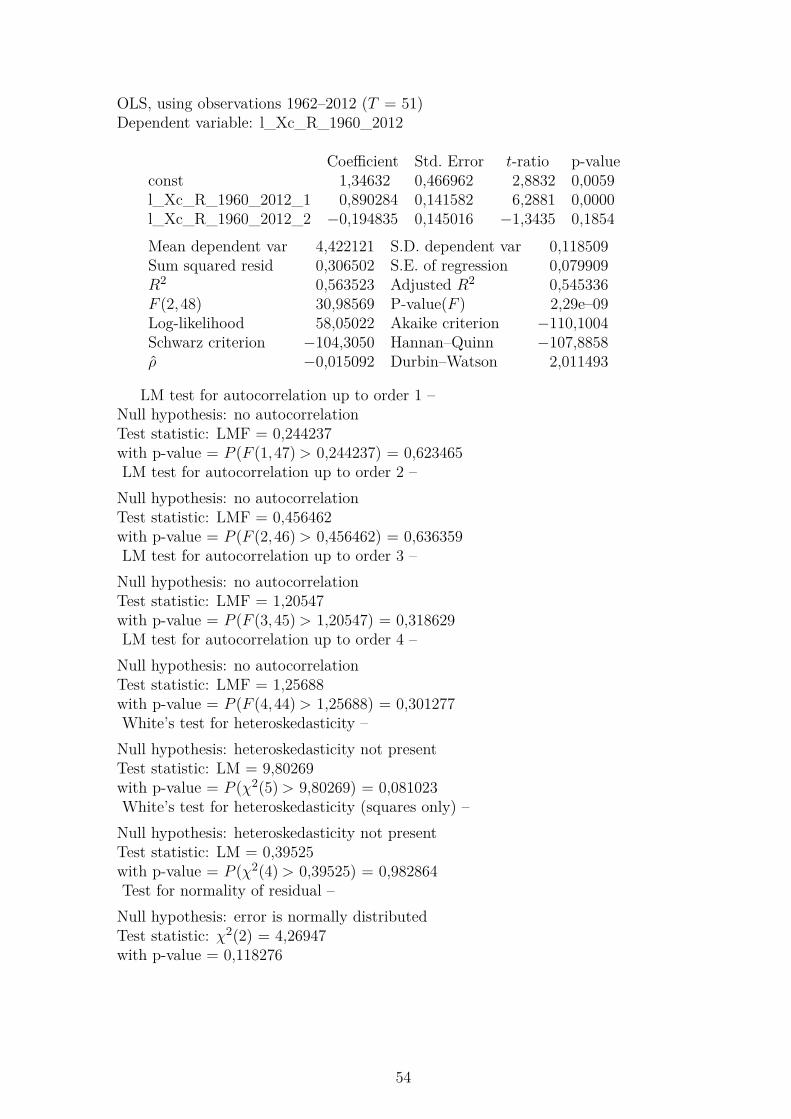
5.4 1960 to 2012
5.4.1 Unit-Root
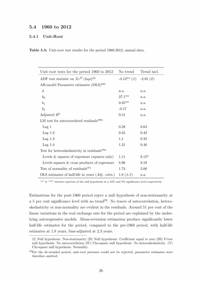
Table 5.5: Unit-root test results for the period 1960-2012, annual data.
Unit root tests for the period 1960 to 2012 No trend Trend incl.
ADF test statistic on XcR (lags)(I) -3.13** (3 ) -2.85 (0 )AR-model Parameter estimates (OLS)(II)
d n.a. n.a.b0 27.1** n.a.b1 0.85** n.a.b2 -0.17 n.a.
Adjusted R2 0.51 n.a.LM test for autocorrelated residuals(III)
Levels & squares of regressors (squares only) 1.11 8.13*Levels squares & cross products of regressors 8.96 9.19
Test of normality of residuals(V) 1.74 2.06OLS estimates of half-life in years (Adj. estm.) 1.8 (2.3 ) n.a.
“*” & ”**” denotes rejection of the null hypothesis at a 10% and 5% significance level respectively
Estimations for the post-1960 period reject a null hypothesis of non-stationarity ata 5 per cent significance level with no trend24. No traces of autocorrelation, hetero-skedasticity or non-normality are evident in the residuals. Around 51 per cent of thelinear variations in the real exchange rate for the period are explained by the under-lying autoregressive models. Mean-reversion estimation produce significantly lowerhalf-life estimates for the period, compared to the pre-1960 period, with half-lifeestimates at 1.8 years, bias-adjusted at 2.3 years.
(I) Null hypothesis: Non-stationarity (II) Null hypothesis: Coefficiant equal to zero (III) F-testnull hypothesis: No autocorrelation (IV) Chi-square null hypothesis: No heteroskedasticity. (V)Chi-square null hypothesis: Normality.
24For the de-trended period, unit-root presence could not be rejected, parameter estimates weretherefore omitted.
26
5.4.2 Cointegration
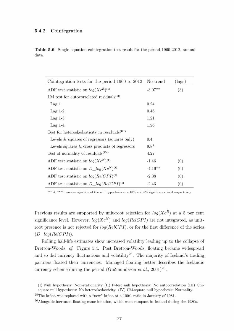
Table 5.6: Single-equation cointegration test result for the period 1960-2012, annualdata.
Cointegration tests for the period 1960 to 2012 No trend (lags)
ADF test statistic on log(XcR)(I) -3.07** (3)LM test for autocorrelated residuals(II)
Lag 1 0.24Lag 1-2 0.46Lag 1-3 1.21Lag 1-4 1.26
Test for heteroskedasticity in residuals(III)
Levels & squares of regressors (squares only) 0.4Levels squares & cross products of regressors 9.8*
Test of normality of residuals(IV) 4.27
ADF test statistic on log(XcN )(I) -1.46 (0)
ADF test statistic on D_log(XcN )(I) -4.16** (0)
ADF test statistic on log(RelCPI)(I) -2.38 (0)
ADF test statistic on D_log(RelCPI)(I) -2.43 (0)
“*” & ”**” denotes rejection of the null hypothesis at a 10% and 5% significance level respectively
Previous results are supported by unit-root rejection for log(XcR) at a 5 per centsignificance level. However, log(XcN ) and log(RelCPI) are not integrated, as unit-root presence is not rejected for log(RelCPI), or for the first difference of the series(D_log(RelCPI)).
Rolling half-life estimates show increased volatility leading up to the collapse ofBretton-Woods, cf. Figure 5.4. Post Bretton-Woods, floating became widespreadand so did currency fluctuations and volatility25. The majority of Iceland’s tradingpartners floated their currencies. Managed floating better describes the Icelandiccurrency scheme during the period (Guðmundsson et al., 2001)26.
(I) Null hypothesis: Non-stationarity (II) F-test null hypothesis: No autocorrelation (III) Chi-square null hypothesis: No heteroskedasticity. (IV) Chi-square null hypothesis: Normality.
25The króna was replaced with a “new” króna at a 100:1 ratio in January of 1981.26Alongside increased floating came inflation, which went rampant in Iceland during the 1980s.
27
0
2
4
6
8
10
1960 1965 1970 1975 1980 1985 1990
Yea
rs
OLS Rolling-Regression Estimates of Half-LivesBias-Adjusted OLS Rolling-Regression Estimates of Half-Lives
Figure 5.4: OLS estimates of half-lives in a 20-year rolling-window regression ofAR(2)-model for XcR. Period 1960 to 1992, annual frequency.
A considerable difference between unadjusted half-life estimates (solid line) andthe bias-adjusted half-life estimates (dotted line) is visible. Unadjusted estimatesshow no dramatic changes during the period27. Bias-adjusted estimates show a sub-stantial increase in half-life duration early in the period, peaking around 1970, withclose to 9 year estimates, before slowly subsiding from then on28.
27In early 1990 a national stability pact was signed. The pact was an agreement between the labourforce and the Government, calling for an end to the wage-price spiral caused by wage demandson top of increasing prices. Formal Government policy emphasizing exchange rate stability at thesame time, drove inflation down. Relative stability ensued (Snævarr, 1993).
28Price Indexation was implemented in the early 1980s, might help explain lower half-life estimatespost-1980.
28
5.5 Monthly Data
5.5.1 Unit-Root
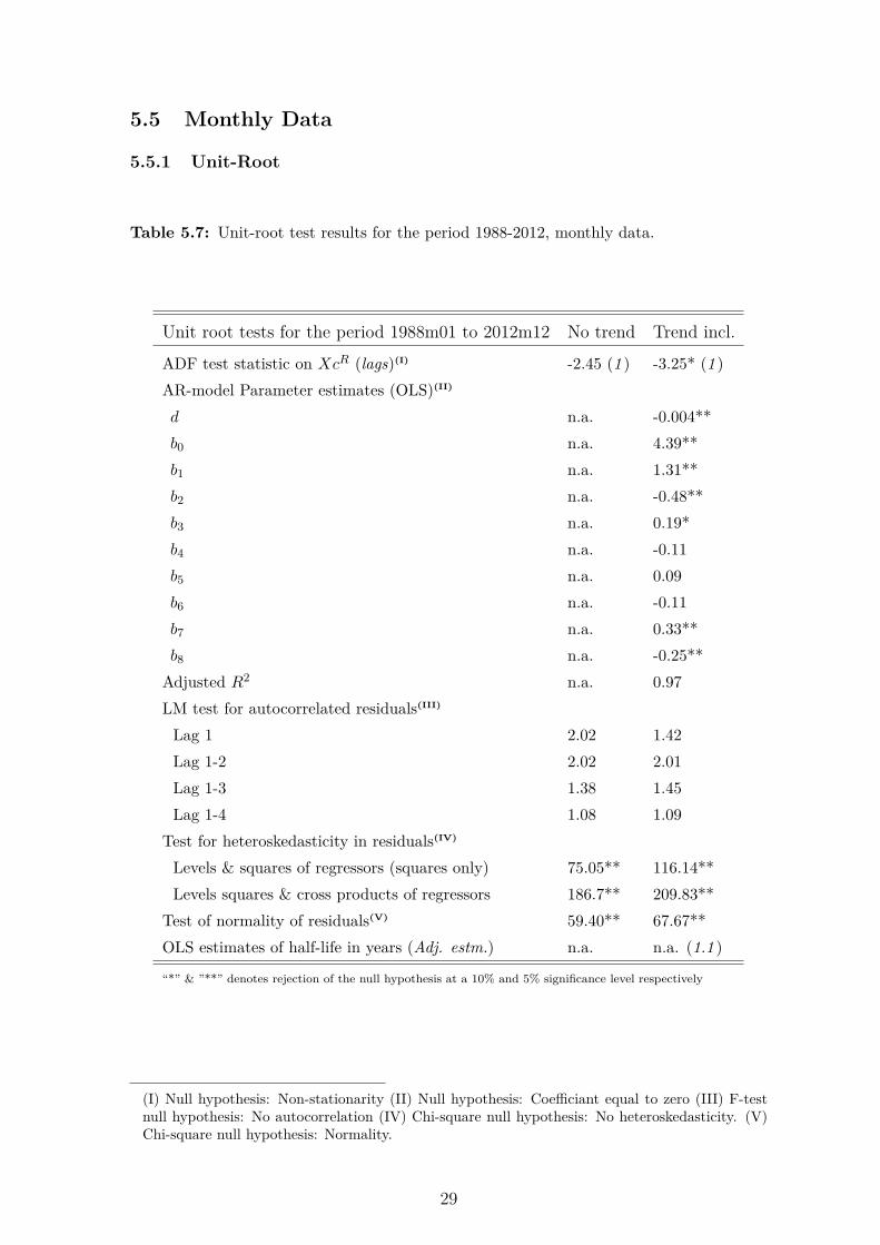
Table 5.7: Unit-root test results for the period 1988-2012, monthly data.
Unit root tests for the period 1988m01 to 2012m12 No trend Trend incl.
ADF test statistic on XcR (lags)(I) -2.45 (1 ) -3.25* (1 )AR-model Parameter estimates (OLS)(II)
Levels & squares of regressors (squares only) 75.05** 116.14**Levels squares & cross products of regressors 186.7** 209.83**
Test of normality of residuals(V) 59.40** 67.67**OLS estimates of half-life in years (Adj. estm.) n.a. n.a. (1.1 )
“*” & ”**” denotes rejection of the null hypothesis at a 10% and 5% significance level respectively
(I) Null hypothesis: Non-stationarity (II) Null hypothesis: Coefficiant equal to zero (III) F-testnull hypothesis: No autocorrelation (IV) Chi-square null hypothesis: No heteroskedasticity. (V)Chi-square null hypothesis: Normality.
29
Using monthly data, non-stationarity is rejected at a 10 per cent significance level forthe period, with trend included29. No traces of autocorrelation are evident; however,the presence of heteroskedasticity and non-normality of the residuals cannot be rejec-ted. The underlying univariate autoregressive models explain around 97 per cent ofthe linear variation in the real effective exchange rate for the period. Bias-adjustedhalf-life estimates are around 1.1 years, in duration.
The negative sign for the time trend parameter is statistically significant. Itcould indicate that Iceland’s competitiveness relative to its trading partners declinedduring the period. Another explanation might be due to the fact that carry tradewas prevalent during a large portion of the period. High interest rates in Iceland,during the so-called “boom years” attracted significant capital inflows, resulting ina considerable appreciation of the ISK. Such effects on exchange rates caused bycapital movements, not involving trade with goods, are not accounted for in the PPPframework30.
A 10-year rolling window of half-life estimates, shows substantial fall in half-lifeduration, after the floating of the ISK in early 2001 (cf. Figure 5.5), from estimatesjust over two years in duration, down to 10 months. A sharp rise noticeable at theend of 2008, when the global recession struck.
0
1
2
3
4
5
1998 2000 2002 2004 2006 2008 2010 2012
Yea
rs
OLS Rolling-Regression Estimates of Half-Lives
Figure 5.5: OLS estimates of half-lives in a 120-month rolling-window regression ofAR(2)-model for XcR. Period 1998 to 2012, monthly frequency.
29For the period without a trend parameter, unit-root presence could not be rejected, parameterestimates were therefore omitted.
30Cf. uncovered interest rate parity discussion in Section 2.
30
Two sharp peaks in late 2005 and early 2006, are likely caused by a so-called mini-crisisthat occurred at the time when the Icelandic banks began to attract internationalattention, due to critical coverage concerning they’re rapid growth in previous years(Guðmundsson, 2010).
5.5.2 Cointegration
Table 5.8: Single-equation cointegration test result for the period 1988-2012, monthlydata
Cointegration tests for the period 1988m01 to 2012m12 No trend (lags)
ADF test statisitc on log(XcR)(I) -2.22 (1)LM test for autocorrelated residuals(II)
Lag 1 2.01Lag 1-2 1.99Lag 1-3 1.62Lag 1-4 1.32
Test for heteroskedasticity in residuals(III)
Levels & squares of regressors (squares only) 106.28**Levels squares & cross products of regressors 216.54**
Test of normality of residuals(IV) 125.23**
ADF test statistic on log(XcN )(I) -1.419 (1)
ADF test statistic on D_log(XcN )(I) -10.80** (1)
ADF test statistic on log(RelCPI)(I) -1.64 (0)
ADF test statistic on D_log(RelCPI)(I) -10.62** (0)
“*” & ”**” denotes rejection of the null hypothesis at a 10% and 5% significance level respectively
Results from cointegration tests contradict previous results for the period. Station-arity is rejected for log(XcR). Unit-root presence in log(XcN ) and log(RelCPI),cannot be rejected, as well. The first differences of both variables reject unit-rootpresence, which indicates first order integration (I(1)), between the two series, butcointegration relationship does not exists.
(I) Null hypothesis: Non-stationarity (II) F-test null hypothesis: No autocorrelation (III) Chi-square null hypothesis: No heteroskedasticity. (IV) Chi-square null hypothesis: Normality.
31
6 Conclusion
This study has explored the validity of the purchasing power parity in the case ofIceland. New historical nominal- and real effective exchange rate indices were con-structed for the Icelandic króna, covering the period from 1895 through 2012. Theindices are based on annual data for the period between 1895 and 1988 and monthlydata from 1988 through 2012. They are constructed as geometrically weighted chainindices with current trade weights based on Iceland’s foreign trade in goods. Con-sumer prices (CPI) are used for deflators. The annual data are based on 13 of Ice-land’s largest trading partners, which accounted for at least 70 per cent of Iceland’stotal foreign trade in good each year during the period. For the monthly data, twocountries are added to the previous list of trading partners. Adding up to a total of15 of Iceland’s largest trading partners, which accounted for at least 64 per cent ofIceland’s total foreign trade in goods each month throughout the period.
For empirical estimation, unit-root and cointegration tests were performed on thenew time-series as a whole, and for two sub-periods that emerged after structuralbreak estimation revealed a breakpoint at 1960. Empirical tests were also performedseparately for the monthly data. The mean-reversion from PPP deviation was ana-lysed via autoregressive models, with half-life calculations using ordinary least squares(OLS) parameter estimates.
The results of unit-root and cointegration tests support long-run relative purchas-ing power parity convergence for Iceland. Estimations from both sub-periods showedsimilar results in support of PPP convergence31. Contradicting test results for thepost-1988 period, indicates a failure of PPP convergence for that period.
Half-lives for the period as a whole, are estimated at around four years in duration,pre-1960 half-lives are also estimated at around four years. The post-1960 periodproduces slightly lower half-life estimates, at around two years in length.
The most rapid mean-reversion is seen in the floating period between 2001 and2008, with half-life estimates around 10 months. Excluding the floating period theinter-war and post-1981 periods show the most rapid mean reversion, with half-lifeestimates ranging from 18 to 24 months. The inter-war period is also the least volatilein the ISK’s history, relative to the trading countries32.
31Stationarity is rejected for both de-trended sub-periods individually, but not for the period as awhole, which might be explained by a structural break presence at 1960.
32Unfortunately rolling estimates do not extend back further than 1915 due to data shortage. His-torically, the pre-1914 period was characterized by relative stability. Iceland was under Danish
32
The results are consistent with results from similar studies on purchasing powerparity. Evidence in support of PPP validation in the long run is found, with half-lifeestimates from PPP deviations that fall right in the middle of the average half-lifeduration of 3-5 years, seen in similar studies (Rogoff, 1996). The relatively lowhalf-life estimates in the post-Bretton-Woods are also consistent with the results ofCashin & McDermott (2003). They concluded that shocks to the real exchange ratedo not appear to be very persistent in the case of the Icelandic króna, relative to realexchange rates of other currencies they examined.
The various tests for relative PPP in this study have been simple and should beconsidered as a first exploratory examination of the new historical time-series for thereal effective exchange rate of the ISK. A combination of the PPP and UIP frameworkfor estimation, might shed light on the results obtained here, especially for the periodbetween 2001 and 2008. For a robustness review of the results proposed here, anon-linear framework using non-aggregated deflator indices as suggested by Taylor(2004), could prove an interesting next step in purchasing power parity examinationfor Iceland.
rule and was therefore, by extension, a part of the Nordic Council Monetary Union, which meantthat all the Nordic currencies, i.e. the Danish-, Norwegian-, Swedish- and Icelandic Krona hadthe same value. This was during the classical gold standard period, when Nordic and most tradingpartner’s currencies were pegged to gold (Guðmundsson et al., 2001).
33
I Appendix
Annual data:Bilateral exchange rates for the Danish krona vis-à-vis Finland, France, Germany,Italy, Japan, the Netherlands, Norway, Portugal, Spain, Sweden, the UK, and theUS, for the period 1895-1988 were obtained from Abildgren (2004). Based on anassumption of perfect international arbitrage cross-currency calculations were madevis-à-vis the Icelandic króna and other currencies, using the bilateral exchange rateof the ISK vis-à-vis the Danish krone, with an exception during the period 9 April1940 to 8 September 1945, when the US dollar is used as a cross reference due tothe quotation suspension of the Danish krone. Official exchange rate quotations forthe ISK versus foreign currencies began on 13 June 1922. Exchange rates before thatdate are calculated from the króna’s gold value (Iceland historical statistics, 1997).Consumer Price indices for Denmark, Finland, France, Germany, Italy, Japan, theNetherlands, Norway, Portugal, Spain, Sweden, the UK, and the US covering theperiod 1895 to 1987 were obtained from Abildgren (2004). The Icelandic consumerprice index is constructed for the period by linking several different price indices, withthe aim of presenting an index of general prices. 1849–98: Price index based on abasket of 27 selected domestic commodities and imported goods. 1899 to 1938: Priceindex 1899 to 1912 based on sources from the Laugarnes Leprosery (Reykjavík); 1913is an estimate; the years 1914 to 1938 are based on price observations of StatisticsIceland made in July 1914 and October each year from 1914 to 1938. 1939 to 1988:Consumer price index excluding housing costs, by Statistics Iceland. Source: IcelandHistorical Statistics, 1997.External trade data for Denmark, Finland, France, Germany, Italy, Japan, the Neth-erlands, Norway, Portugal, Spain, Sweden, the UK, and the US were collected. Im-ports are at cif value and exports at fob value. Data for the Faeroe Islands areincluded with the data for Denmark. Data for East Germany are included in thedata for Germany 1946 to 1988 (Iceland Historical Statistics, 1997)Terms of trade. Data source: Iceland Historical Statistics, 1997 & the Central Bankof Iceland, 2013.Official real exchange rate (REER). Data source: Central Bank of Iceland, 2013(www.cb.is).Gross Domestic Product. GNP is replaced by the GDP post-1945. GNP is in the
34
table deflated with a weighted index composed of the consumer price index (2/3) andbuilding cost index (1/3). Iceland Historical Statistics (1997).
Monthly data:Bilateral exchange rates for the Icelandic króna vis-à-vis Belgium, Denmark, Finland,France, Germany, Italy, Japan, the Netherlands, Norway, Portugal, Spain, Sweden,Switzerland, the UK, and the US were obtained from the Central Bank of Iceland(2013). In September 2002 the following countries adopted the euro: France, theNetherlands, Portugal, Spain, Germany, Belgium, Finland and Italy. From 2002onwards, the exchange rates for those countries are calculated on basis of the euroexchange rate versus the Icelandic króna and exchange rates of the euro vis-à-vis thecurrencies of the previously listed countries.External trade data for Belgium, Denmark, Finland, France, Germany, Italy, Japan,the Netherlands, Norway, Portugal, Spain, Sweden, Switzerland, the UK, and the USwere collected. Data for the Faeroe Islands and Greenland are included in the datafor Denmark. Imports are at cif value and exports at fob value (Statistics Iceland,2013).Consumer Price indices (CPI) and Harmonized Indices of Consumer Price (HICP)for Belgium, Denmark, Finland, France, Germany, Italy, Japan, the Netherlands,Norway, Portugal, Spain, Sweden, Switzerland, the UK, the US, and Iceland werecollected. Data source: OECD database (2013) & BIS database (2013). HICP re-place normal CPI’s when available. The Harmonized consumer price index providesa standard measurement for the index and is therefore a better choice as deflator forthis kind of survey. HICP data do not exist prior to January 1990. To incorporateHICP into the CPI in order to construct one continuous time-series, relative changein each country’s CPI is applied to the starting value of the HICP and calculatedbackwards. The starting date for HICP measurements varies from country to coun-try. HICP data are available for Denmark, France, Netherlands, Portugal, Sweden,the UK, Finland, and Italy from January 1990, for Spain from January 1992, forIceland and Germany from January 1995, for Belgium from January 1991, for the USfrom December 1997, for Japan and Norway from January 1996, and for Switzerlandfrom December 2004. HICP are consumer price indices compiled on the basis of aharmonised coverage and methodology. For further details, cf. Harmonized Indicesof Consumer Prices. A Short Guide for Users (HICPs), 2004.
35
II Appendix
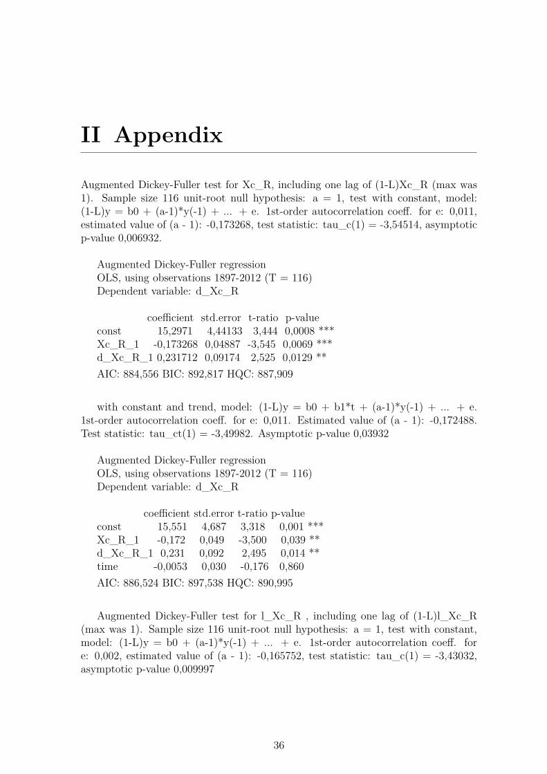
Augmented Dickey-Fuller test for Xc_R, including one lag of (1-L)Xc_R (max was1). Sample size 116 unit-root null hypothesis: a = 1, test with constant, model:(1-L)y = b0 + (a-1)*y(-1) + ... + e. 1st-order autocorrelation coeff. for e: 0,011,estimated value of (a - 1): -0,173268, test statistic: tau_c(1) = -3,54514, asymptoticp-value 0,006932.
Augmented Dickey-Fuller test for l_Xc_R , including one lag of (1-L)l_Xc_R(max was 1). Sample size 116 unit-root null hypothesis: a = 1, test with constant,model: (1-L)y = b0 + (a-1)*y(-1) + ... + e. 1st-order autocorrelation coeff. fore: 0,002, estimated value of (a - 1): -0,165752, test statistic: tau_c(1) = -3,43032,asymptotic p-value 0,009997
Augmented Dickey-Fuller test for l_Xc_N, including one lag of (1-L)l_Xc_N(max was 1). Sample size 116 unit-root, null hypothesis: a = 1, Test with constant,model: (1-L)y = b0 + (a-1)*y(-1) + ... + e. 1st-order autocorrelation coeff. fore: -0,024, estimated value of (a - 1): 0,00599407, test statistic: tau_c(1) = 1,11729,asymptotic p-value 0,9977
Dickey-Fuller test for d_l_Xc_N. sample size 116 unit-root, null hypothesis: a =1. Test with constant, model: (1-L)y = b0 + (a-1)*y(-1) + e. 1st-order autocorrela-tion coeff. for e: -0,034, estimated value of (a - 1): -0,626694, test statistic: tau_c(1)= -7,21607, p-value 3,547e-009
Dickey-Fuller regressionOLS, using observations 1897-2012 (T = 116)Dependent variable: d_d_l_Xc_N
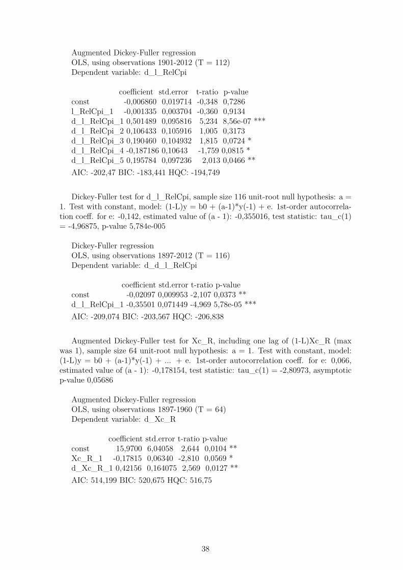
Augmented Dickey-Fuller test for l_RelCpi, including 5 lags of (1-L)l_RelCpi(max was 5). Sample size 112 unit-root null hypothesis: a = 1, test with constant,model: (1-L)y = b0 + (a-1)*y(-1) + ... + e. 1st-order autocorrelation coeff. fore: 0,029, lagged differences: F(5, 105) = 18,059 [0,0000], estimated value of (a - 1):-0,00133539, test statistic: tau_c(1) = -0,360434, asymptotic p-value 0,9134
Dickey-Fuller test for d_l_RelCpi, sample size 116 unit-root null hypothesis: a =1. Test with constant, model: (1-L)y = b0 + (a-1)*y(-1) + e. 1st-order autocorrela-tion coeff. for e: -0,142, estimated value of (a - 1): -0,355016, test statistic: tau_c(1)= -4,96875, p-value 5,784e-005
Dickey-Fuller regressionOLS, using observations 1897-2012 (T = 116)Dependent variable: d_d_l_RelCpi
Augmented Dickey-Fuller test for Xc_R, including one lag of (1-L)Xc_R (maxwas 1), sample size 64 unit-root null hypothesis: a = 1. Test with constant, model:(1-L)y = b0 + (a-1)*y(-1) + ... + e. 1st-order autocorrelation coeff. for e: 0,066,estimated value of (a - 1): -0,178154, test statistic: tau_c(1) = -2,80973, asymptoticp-value 0,05686
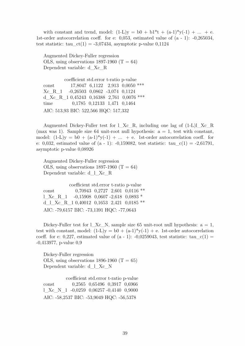
Augmented Dickey-Fuller test for l_Xc_R, including one lag of (1-L)l_Xc_R(max was 1). Sample size 64 unit-root null hypothesis: a = 1, test with constant,model: (1-L)y = b0 + (a-1)*y(-1) + ... + e. 1st-order autocorrelation coeff. fore: 0,032, estimated value of (a - 1): -0,159082, test statistic: tau_c(1) = -2,61791,asymptotic p-value 0,08926
Dickey-Fuller test for l_Xc_N, sample size 65 unit-root null hypothesis: a = 1,test with constant, model: (1-L)y = b0 + (a-1)*y(-1) + e. 1st-order autocorrelationcoeff. for e: 0,227, estimated value of (a - 1): -0,0259043, test statistic: tau_c(1) =-0,413977, p-value 0,9
Dickey-Fuller regressionOLS, using observations 1896-1960 (T = 65)Dependent variable: d_l_Xc_N
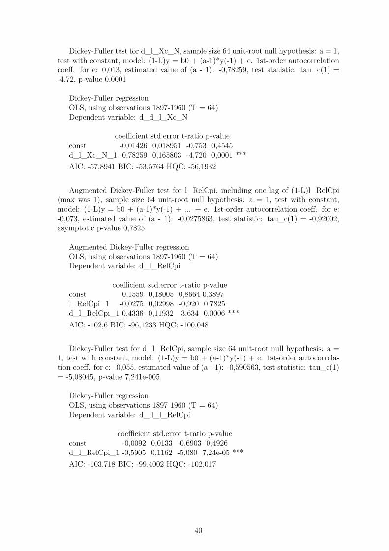
Dickey-Fuller test for d_l_Xc_N, sample size 64 unit-root null hypothesis: a = 1,test with constant, model: (1-L)y = b0 + (a-1)*y(-1) + e. 1st-order autocorrelationcoeff. for e: 0,013, estimated value of (a - 1): -0,78259, test statistic: tau_c(1) =-4,72, p-value 0,0001
Dickey-Fuller regressionOLS, using observations 1897-1960 (T = 64)Dependent variable: d_d_l_Xc_N
Augmented Dickey-Fuller test for l_RelCpi, including one lag of (1-L)l_RelCpi(max was 1), sample size 64 unit-root null hypothesis: a = 1, test with constant,model: (1-L)y = b0 + (a-1)*y(-1) + ... + e. 1st-order autocorrelation coeff. for e:-0,073, estimated value of (a - 1): -0,0275863, test statistic: tau_c(1) = -0,92002,asymptotic p-value 0,7825
Dickey-Fuller test for d_l_RelCpi, sample size 64 unit-root null hypothesis: a =1, test with constant, model: (1-L)y = b0 + (a-1)*y(-1) + e. 1st-order autocorrela-tion coeff. for e: -0,055, estimated value of (a - 1): -0,590563, test statistic: tau_c(1)= -5,08045, p-value 7,241e-005
Dickey-Fuller regressionOLS, using observations 1897-1960 (T = 64)Dependent variable: d_d_l_RelCpi
Augmented Dickey-Fuller test for Xc_R_1960_2012including 3 lags of (1-L)Xc_R_1960_2012 (max was 3), sample size 49 unit-root nullhypothesis: a = 1, test with constant, model: (1-L)y = b0 + (a-1)*y(-1) + ... +e. 1st-order autocorrelation coeff. for e: -0,016, lagged differences: F(3, 44) = 1,433[0,2459], estimated value of (a - 1): -0,482749, test statistic: tau_c(1) = -3,13359,asymptotic p-value 0,02419
Dickey-Fuller test for Xc_R_1960_2012, sample size 52 unit-root null hypothesis:a = 1, with constant and trend, model: (1-L)y = b0 + b1*t + (a-1)*y(-1) + e. 1st-order autocorrelation coeff. for e: 0,085, estimated value of (a - 1): -0,279732, teststatistic: tau_ct(1) = -2,85408, p-value 0,1856
Dickey-Fuller regressionOLS, using observations 1961-2012 (T = 52)Dependent variable: d_Xc_R_1960_2012
Augmented Dickey-Fuller test for l_Xc_R_1960_2012, including 3 lags of (1-L)l_Xc_R_1960_2012 (max was 3), sample size 49 unit-root null hypothesis: a= 1, test with constant, model: (1-L)y = b0 + (a-1)*y(-1) + ... + e. 1st-orderautocorrelation coeff. for e: -0,010, lagged differences: F(3, 44) = 1,573 [0,2094],estimated value of (a - 1): -0,46579, test statistic: tau_c(1) = -3,06756, asymptoticp-value 0,02907
Dickey-Fuller test for l_Xc_N_1960_2012, sample size 52 unit-root null hypo-thesis: a = 1, test with constant, model: (1-L)y = b0 + (a-1)*y(-1) + e. 1st-orderautocorrelation coeff. for e: 0,459, estimated value of (a - 1): -0,0141904, test stat-istic: tau_c(1) = -1,459, p-value 0,5463
Dickey-Fuller regressionOLS, using observations 1961-2012 (T = 52)Dependent variable: d_l_Xc_N_1960_2012
Dickey-Fuller test for d_l_Xc_N_1960_2012, sample size 51 unit-root null hy-pothesis: a = 1, test with constant, model: (1-L)y = b0 + (a-1)*y(-1) + e. 1st-orderautocorrelation coeff. for e: -0,027, estimated value of (a - 1): -0,524971, test stat-istic: tau_c(1) = -4,15546, p-value 0,001864
Dickey-Fuller regressionOLS, using observations 1962-2012 (T = 51)Dependent variable: d_d_l_Xc_N_1960_2012
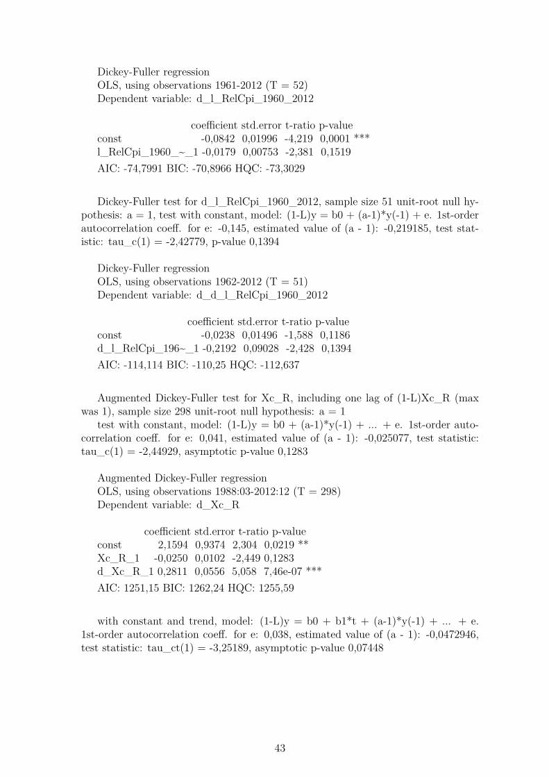
Dickey-Fuller test for l_RelCpi_1960_2012, sample size 52 unit-root null hypo-thesis: a = 1, test with constant, model: (1-L)y = b0 + (a-1)*y(-1) + e. 1st-orderautocorrelation coeff. for e: 0,753, estimated value of (a - 1): -0,0179279, test stat-istic: tau_c(1) = -2,38101, p-value 0,1519
42
Dickey-Fuller regressionOLS, using observations 1961-2012 (T = 52)Dependent variable: d_l_RelCpi_1960_2012
Dickey-Fuller test for d_l_RelCpi_1960_2012, sample size 51 unit-root null hy-pothesis: a = 1, test with constant, model: (1-L)y = b0 + (a-1)*y(-1) + e. 1st-orderautocorrelation coeff. for e: -0,145, estimated value of (a - 1): -0,219185, test stat-istic: tau_c(1) = -2,42779, p-value 0,1394
Dickey-Fuller regressionOLS, using observations 1962-2012 (T = 51)Dependent variable: d_d_l_RelCpi_1960_2012
Augmented Dickey-Fuller test for Xc_R, including one lag of (1-L)Xc_R (maxwas 1), sample size 298 unit-root null hypothesis: a = 1
test with constant, model: (1-L)y = b0 + (a-1)*y(-1) + ... + e. 1st-order auto-correlation coeff. for e: 0,041, estimated value of (a - 1): -0,025077, test statistic:tau_c(1) = -2,44929, asymptotic p-value 0,1283
Augmented Dickey-Fuller test for l_Xc_R, including one lag of (1-L)l_Xc_R(max was 1), sample size 298 unit-root null hypothesis: a = 1, test with constant,model: (1-L)y = b0 + (a-1)*y(-1) + ... + e. 1st-order autocorrelation coeff. fore: 0,045, estimated value of (a - 1): -0,0227047, test statistic: tau_c(1) = -2,2185,asymptotic p-value 0,1997
Augmented Dickey-Fuller test for l_Xc_N, including one lag of (1-L)l_Xc_N(max was 1), sample size 298 unit-root null hypothesis: a = 1, test with constant,model: (1-L)y = b0 + (a-1)*y(-1) + ... + e. 1st-order autocorrelation coeff. for e:0,045, estimated value of (a - 1): -0,00648686, test statistic: tau_c(1) = -1,41897,asymptotic p-value 0,5746
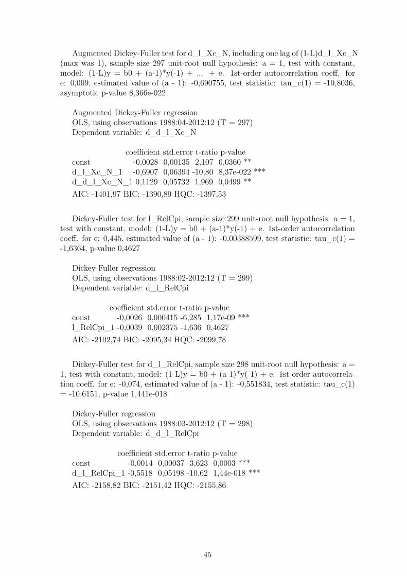
Augmented Dickey-Fuller test for d_l_Xc_N, including one lag of (1-L)d_l_Xc_N(max was 1), sample size 297 unit-root null hypothesis: a = 1, test with constant,model: (1-L)y = b0 + (a-1)*y(-1) + ... + e. 1st-order autocorrelation coeff. fore: 0,009, estimated value of (a - 1): -0,690755, test statistic: tau_c(1) = -10,8036,asymptotic p-value 8,366e-022
Dickey-Fuller test for l_RelCpi, sample size 299 unit-root null hypothesis: a = 1,test with constant, model: (1-L)y = b0 + (a-1)*y(-1) + e. 1st-order autocorrelationcoeff. for e: 0,445, estimated value of (a - 1): -0,00388599, test statistic: tau_c(1) =-1,6364, p-value 0,4627
Dickey-Fuller regressionOLS, using observations 1988:02-2012:12 (T = 299)Dependent variable: d_l_RelCpi
Dickey-Fuller test for d_l_RelCpi, sample size 298 unit-root null hypothesis: a =1, test with constant, model: (1-L)y = b0 + (a-1)*y(-1) + e. 1st-order autocorrela-tion coeff. for e: -0,074, estimated value of (a - 1): -0,551834, test statistic: tau_c(1)= -10,6151, p-value 1,441e-018
Dickey-Fuller regressionOLS, using observations 1988:03-2012:12 (T = 298)Dependent variable: d_d_l_RelCpi
Mean dependent var 88,43992 S.D. dependent var 21,48312Sum squared resid 13219,81 S.E. of regression 10,81617R2 0,750924 Adjusted R2 0,746515F (2,113) 170,3380 P-value(F ) 7,81e–35Log-likelihood −439,2780 Akaike criterion 884,5560Schwarz criterion 892,8168 Hannan–Quinn 887,9094ρ̂ 0,010775 Durbin’s h 0,603017
LM test for autocorrelation up to order 1 –Null hypothesis: no autocorrelationTest statistic: LMF = 0,241768with p-value = P (F (1,112)> 0,241768) = 0,623894
LM test for autocorrelation up to order 2 –Null hypothesis: no autocorrelationTest statistic: LMF = 0,16029with p-value = P (F (2,111)> 0,16029) = 0,852093
LM test for autocorrelation up to order 3 –Null hypothesis: no autocorrelationTest statistic: LMF = 0,194025with p-value = P (F (3,110)> 0,194025) = 0,900275
LM test for autocorrelation up to order 4 –Null hypothesis: no autocorrelationTest statistic: LMF = 0,498338with p-value = P (F (4,109)> 0,498338) = 0,73698
White’s test for heteroskedasticity –Null hypothesis: heteroskedasticity not presentTest statistic: LM = 25,2318with p-value = P (χ2(5)> 25,2318) = 0,00012568
White’s test for heteroskedasticity (squares only) –Null hypothesis: heteroskedasticity not presentTest statistic: LM = 24,6408with p-value = P (χ2(4)> 24,6408) = 5,94063e-005
Test for normality of residual –Null hypothesis: error is normally distributedTest statistic: χ2(2) = 73,7181with p-value = 9,82452e-017
46
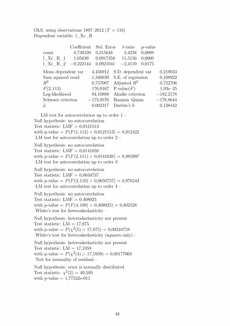
OLS, using observations 1897–2012 (T = 116)Dependent variable: Xc_R
LM test for autocorrelation up to order 1 –Null hypothesis: no autocorrelationTest statistic: LMF = 0,248408with p-value = P (F (1,111)> 0,248408) = 0,619185LM test for autocorrelation up to order 2 –Null hypothesis: no autocorrelationTest statistic: LMF = 0,166767with p-value = P (F (2,110)> 0,166767) = 0,84661LM test for autocorrelation up to order 3 –Null hypothesis: no autocorrelationTest statistic: LMF = 0,17564with p-value = P (F (3,109)> 0,17564) = 0,912687LM test for autocorrelation up to order 4 –Null hypothesis: no autocorrelationTest statistic: LMF = 0,518602with p-value = P (F (4,108)> 0,518602) = 0,722216White’s test for heteroskedasticity –Null hypothesis: heteroskedasticity not presentTest statistic: LM = 28,4342with p-value = P (χ2(9)> 28,4342) = 0,000806822White’s test for heteroskedasticity (squares only) –Null hypothesis: heteroskedasticity not presentTest statistic: LM = 24,9801with p-value = P (χ2(6)> 24,9801) = 0,000344368Test for normality of residual –Null hypothesis: error is normally distributedTest statistic: χ2(2) = 72,7118with p-value = 1,62494e-016
47
OLS, using observations 1897–2012 (T = 116)Dependent variable: l_Xc_R
LM test for autocorrelation up to order 1 –Null hypothesis: no autocorrelationTest statistic: LMF = 0,0121513with p-value = P (F (1,112)> 0,0121513) = 0,912422LM test for autocorrelation up to order 2 –Null hypothesis: no autocorrelationTest statistic: LMF = 0,0141038with p-value = P (F (2,111)> 0,0141038) = 0,985997LM test for autocorrelation up to order 3 –Null hypothesis: no autocorrelationTest statistic: LMF = 0,0650737with p-value = P (F (3,110)> 0,0650737) = 0,978243LM test for autocorrelation up to order 4 –Null hypothesis: no autocorrelationTest statistic: LMF = 0,408025with p-value = P (F (4,109)> 0,408025) = 0,802528White’s test for heteroskedasticity –Null hypothesis: heteroskedasticity not presentTest statistic: LM = 17,875with p-value = P (χ2(5)> 17,875) = 0,00310719White’s test for heteroskedasticity (squares only) –Null hypothesis: heteroskedasticity not presentTest statistic: LM = 17,1959with p-value = P (χ2(4)> 17,1959) = 0,00177069Test for normality of residual –Null hypothesis: error is normally distributedTest statistic: χ2(2) = 49,509with p-value = 1,77522e-011
48
OLS, using observations 1897–1960 (T = 64)Dependent variable: Xc_R
LM test for autocorrelation up to order 1 –Null hypothesis: no autocorrelationTest statistic: LMF = 1,01045with p-value = P (F (1,60)> 1,01045) = 0,318832LM test for autocorrelation up to order 2 –Null hypothesis: no autocorrelationTest statistic: LMF = 0,59232with p-value = P (F (2,59)> 0,59232) = 0,556298LM test for autocorrelation up to order 3 –Null hypothesis: no autocorrelationTest statistic: LMF = 0,482729with p-value = P (F (3,58)> 0,482729) = 0,695575LM test for autocorrelation up to order 4 –Null hypothesis: no autocorrelationTest statistic: LMF = 0,50306with p-value = P (F (4,57)> 0,50306) = 0,733583White’s test for heteroskedasticity –Null hypothesis: heteroskedasticity not presentTest statistic: LM = 13,5652with p-value = P (χ2(5)> 13,5652) = 0,0186207White’s test for heteroskedasticity (squares only) –Null hypothesis: heteroskedasticity not presentTest statistic: LM = 13,3138with p-value = P (χ2(4)> 13,3138) = 0,00983987Test for normality of residual –Null hypothesis: error is normally distributedTest statistic: χ2(2) = 44,2471with p-value = 2,46531e-010
49
OLS, using observations 1897–1960 (T = 64)Dependent variable: Xc_R
LM test for autocorrelation up to order 1 –Null hypothesis: no autocorrelationTest statistic: LMF = 0,528047with p-value = P (F (1,59)> 0,528047) = 0,470302LM test for autocorrelation up to order 2 –Null hypothesis: no autocorrelationTest statistic: LMF = 0,443305with p-value = P (F (2,58)> 0,443305) = 0,644068LM test for autocorrelation up to order 3 –Null hypothesis: no autocorrelationTest statistic: LMF = 0,409194with p-value = P (F (3,57)> 0,409194) = 0,746989LM test for autocorrelation up to order 4 –Null hypothesis: no autocorrelationTest statistic: LMF = 0,378875with p-value = P (F (4,56)> 0,378875) = 0,822779White’s test for heteroskedasticity –Null hypothesis: heteroskedasticity not presentTest statistic: LM = 19,6845with p-value = P (χ2(9)> 19,6845) = 0,0199628White’s test for heteroskedasticity (squares only) –Null hypothesis: heteroskedasticity not presentTest statistic: LM = 13,0133with p-value = P (χ2(6)> 13,0133) = 0,0428252Test for normality of residual –Null hypothesis: error is normally distributedTest statistic: χ2(2) = 44,9109with p-value = 1,76895e-010
50
OLS, using observations 1897–1960 (T = 64)Dependent variable: l_Xc_R
LM test for autocorrelation up to order 1 –Null hypothesis: no autocorrelationTest statistic: LMF = 0,245716with p-value = P (F (1,60)> 0,245716) = 0,621918LM test for autocorrelation up to order 2 –Null hypothesis: no autocorrelationTest statistic: LMF = 0,121415with p-value = P (F (2,59)> 0,121415) = 0,885887LM test for autocorrelation up to order 3 –Null hypothesis: no autocorrelationTest statistic: LMF = 0,101124with p-value = P (F (3,58)> 0,101124) = 0,959053LM test for autocorrelation up to order 4 –Null hypothesis: no autocorrelationTest statistic: LMF = 0,191with p-value = P (F (4,57)> 0,191) = 0,942147White’s test for heteroskedasticity –Null hypothesis: heteroskedasticity not presentTest statistic: LM = 10,3855with p-value = P (χ2(5)> 10,3855) = 0,0650219White’s test for heteroskedasticity (squares only) –Null hypothesis: heteroskedasticity not presentTest statistic: LM = 10,2512with p-value = P (χ2(4)> 10,2512) = 0,0364019Test for normality of residual –Null hypothesis: error is normally distributedTest statistic: χ2(2) = 37,3186with p-value = 7,87714e-009
51
OLS, using observations 1962–2012 (T = 51)Dependent variable: Xc_R_1960_2012
LM test for autocorrelation up to order 1 –Null hypothesis: no autocorrelationTest statistic: LMF = 0,277671with p-value = P (F (1,47)> 0,277671) = 0,60071LM test for autocorrelation up to order 2 –Null hypothesis: no autocorrelationTest statistic: LMF = 0,446407with p-value = P (F (2,46)> 0,446407) = 0,642666LM test for autocorrelation up to order 3 –Null hypothesis: no autocorrelationTest statistic: LMF = 1,09831with p-value = P (F (3,45)> 1,09831) = 0,359695LM test for autocorrelation up to order 4 –Null hypothesis: no autocorrelationTest statistic: LMF = 1,20654with p-value = P (F (4,44)> 1,20654) = 0,32158White’s test for heteroskedasticity (squares only) –Null hypothesis: heteroskedasticity not presentTest statistic: LM = 1,11055with p-value = P (χ2(4)> 1,11055) = 0,892595White’s test for heteroskedasticity –Null hypothesis: heteroskedasticity not presentTest statistic: LM = 8,95846with p-value = P (χ2(5)> 8,95846) = 0,110733Test for normality of residual –Null hypothesis: error is normally distributedTest statistic: χ2(2) = 1,74447with p-value = 0,418016
52
OLS, using observations 1961–2012 (T = 52)Dependent variable: Xc_R_1960_2012
LM test for autocorrelation up to order 1 –Null hypothesis: no autocorrelationTest statistic: LMF = 0,644903with p-value = P (F (1,48)> 0,644903) = 0,4259LM test for autocorrelation up to order 2 –Null hypothesis: no autocorrelationTest statistic: LMF = 0,422911with p-value = P (F (2,47)> 0,422911) = 0,657605LM test for autocorrelation up to order 3 –Null hypothesis: no autocorrelationTest statistic: LMF = 0,321171with p-value = P (F (3,46)> 0,321171) = 0,810007LM test for autocorrelation up to order 4 –Null hypothesis: no autocorrelationTest statistic: LMF = 0,477526with p-value = P (F (4,45)> 0,477526) = 0,752004White’s test for heteroskedasticity –Null hypothesis: heteroskedasticity not presentTest statistic: LM = 9,189with p-value = P (χ2(5)> 9,189) = 0,101759White’s test for heteroskedasticity (squares only) –Null hypothesis: heteroskedasticity not presentTest statistic: LM = 8,13327with p-value = P (χ2(4)> 8,13327) = 0,0868165Test for normality of residual –Null hypothesis: error is normally distributedTest statistic: χ2(2) = 2,06003with p-value = 0,357002
53
OLS, using observations 1962–2012 (T = 51)Dependent variable: l_Xc_R_1960_2012
LM test for autocorrelation up to order 1 –Null hypothesis: no autocorrelationTest statistic: LMF = 0,244237with p-value = P (F (1,47)> 0,244237) = 0,623465LM test for autocorrelation up to order 2 –Null hypothesis: no autocorrelationTest statistic: LMF = 0,456462with p-value = P (F (2,46)> 0,456462) = 0,636359LM test for autocorrelation up to order 3 –Null hypothesis: no autocorrelationTest statistic: LMF = 1,20547with p-value = P (F (3,45)> 1,20547) = 0,318629LM test for autocorrelation up to order 4 –Null hypothesis: no autocorrelationTest statistic: LMF = 1,25688with p-value = P (F (4,44)> 1,25688) = 0,301277White’s test for heteroskedasticity –Null hypothesis: heteroskedasticity not presentTest statistic: LM = 9,80269with p-value = P (χ2(5)> 9,80269) = 0,081023White’s test for heteroskedasticity (squares only) –Null hypothesis: heteroskedasticity not presentTest statistic: LM = 0,39525with p-value = P (χ2(4)> 0,39525) = 0,982864Test for normality of residual –Null hypothesis: error is normally distributedTest statistic: χ2(2) = 4,26947with p-value = 0,118276
54
OLS, using observations 1988:09–2012:12 (T = 292)Dependent variable: Xc_R
LM test for autocorrelation up to order 1 –Null hypothesis: no autocorrelationTest statistic: LMF = 2,01786with p-value = P (F (1,282)> 2,01786) = 0,156563LM test for autocorrelation up to order 2 –Null hypothesis: no autocorrelationTest statistic: LMF = 2,02437with p-value = P (F (2,281)> 2,02437) = 0,133999LM test for autocorrelation up to order 3 –Null hypothesis: no autocorrelationTest statistic: LMF = 1,37573with p-value = P (F (3,280)> 1,37573) = 0,250412LM test for autocorrelation up to order 4 –Null hypothesis: no autocorrelationTest statistic: LMF = 1,08183with p-value = P (F (4,279)> 1,08183) = 0,365743White’s test for heteroskedasticity –Null hypothesis: heteroskedasticity not presentTest statistic: LM = 186,716with p-value = P (χ2(44)> 186,716) = 1,69401e-019White’s test for heteroskedasticity (squares only) –Null hypothesis: heteroskedasticity not presentTest statistic: LM = 75,0501with p-value = P (χ2(16)> 75,0501) = 1,28097e-009Test for normality of residual –Null hypothesis: error is normally distributedTest statistic: χ2(2) = 59,4075with p-value = 1,25841e-013
55
OLS, using observations 1988:09–2012:12 (T = 292)Dependent variable: l_Xc_R
LM test for autocorrelation up to order 1 –Null hypothesis: no autocorrelationTest statistic: LMF = 2,00912with p-value = P (F (1,282)> 2,00912) = 0,15746LM test for autocorrelation up to order 2 –Null hypothesis: no autocorrelationTest statistic: LMF = 1,99863with p-value = P (F (2,281)> 1,99863) = 0,137443LM test for autocorrelation up to order 3 –Null hypothesis: no autocorrelationTest statistic: LMF = 1,62489with p-value = P (F (3,280)> 1,62489) = 0,183791LM test for autocorrelation up to order 4 –Null hypothesis: no autocorrelationTest statistic: LMF = 1,32055with p-value = P (F (4,279)> 1,32055) = 0,262451White’s test for heteroskedasticity –Null hypothesis: heteroskedasticity not presentTest statistic: LM = 216,543with p-value = P (χ2(44)> 216,543) = 1,22252e-024White’s test for heteroskedasticity (squares only) –Null hypothesis: heteroskedasticity not presentTest statistic: LM = 106,282with p-value = P (χ2(16)> 106,282) = 2,27342e-015Test for normality of residual –Null hypothesis: error is normally distributedTest statistic: χ2(2) = 125,234with p-value = 6,39354e-028
56
OLS, using observations 1988:09–2012:12 (T = 292)Dependent variable: Xc_R
LM test for autocorrelation up to order 1 –Null hypothesis: no autocorrelationTest statistic: LMF = 1,42423with p-value = P (F (1,281)> 1,42423) = 0,233716LM test for autocorrelation up to order 2 –Null hypothesis: no autocorrelationTest statistic: LMF = 2,01047with p-value = P (F (2,280)> 2,01047) = 0,135855LM test for autocorrelation up to order 3 –Null hypothesis: no autocorrelationTest statistic: LMF = 1,44505with p-value = P (F (3,279)> 1,44505) = 0,229924LM test for autocorrelation up to order 4 –Null hypothesis: no autocorrelationTest statistic: LMF = 1,08877with p-value = P (F (4,278)> 1,08877) = 0,362337White’s test for heteroskedasticity –Null hypothesis: heteroskedasticity not presentTest statistic: LM = 209,833with p-value = P (χ2(54)> 209,833) = 3,11608e-020White’s test for heteroskedasticity (squares only) –Null hypothesis: heteroskedasticity not presentTest statistic: LM = 116,142with p-value = P (χ2(18)> 116,142) = 2,23481e-016Test for normality of residual –Null hypothesis: error is normally distributedTest statistic: χ2(2) = 67,6665with p-value = 2,02491e-015
57
III Appendix
0
10
20
30
40
50
60
1900 1920 1940 1960 1980 2000
%
Imports/GDPExports/GDP
Figure III.1: Total annual share of exports and imports of GDP, each year for theperiod 1901-2012, at current prices. Data source: cf. Appendix I.
50
100
150
200
250
300
350
1900 1920 1940 1960 1980 2000
Xc^RTerms of Trade
1895=100
Figure III.2: Development of the new XcR & terms of trade for Iceland, annualfrequency: 1895 to 2012 (1895=2012). Data source: cf. Appendix I.
58
55
60
65
70
75
80
85
90
95
100
1900 1910 1920 1930 1940 1950 1960 1970 1980
%
Import (annual)Export (annual)
Figure III.3: Share of the exports & imports that are included in this study, of Iceland’stotal exports & imports, each year. 1895 to 1987. Data source: cf. Appendix I.
50
60
70
80
90
100
1990 1995 2000 2005 2010
%
Import (monthly)Export (monthly)
Figure III.4: Share of the exports & imports that are included in this study, of Iceland’stotal exports & imports, each month. 1988 to 2012. Data source: cf. Appendix I.
The drop in annual imports and exports during the 1950s is due to external trade between Icelandand the USSR during the period. USSR is not included in this research.
59
50
60
70
80
90
100
110
1990 1995 2000 2005 2010
REERXc^R
Jan 1988=100
Figure III.5: Comparison of the new real effective exchange rate of the Icelandic króna(XcR) & the official real exchange rate of The Central Bank, monthly frequency: 1988 to2012 (Jan 1988 = 100). Data source: cf. Appendix I & calculations in Section 3.
20
30
40
50
60
70
80
90
100
110
1990 1995 2000 2005 2010
Xc^NRelCPIJan 1988=100
Figure III.6: The new nominal effective króna exchange rate (XcN ) and Relative prices(RelCPI), monthly frequency: 1988 to 2012 (Jan 1988 = 100). Data source: cf.Appendix I & calculations in Section 3.
60
100
150
200
250
300
350
400
1990 1995 2000 2005 2010
CPI^FCPI^I
Jan 1988=100
Figure III.7: Comparison of the Icelandic (CPII) & foreign consumer price indices(CPIF ), monthly frequency: 1988 to 2012 (Jan 1988 = 100). Data source: cf. Appendix I& calculations in Section 3.
4
6
8
10
12
14
16
1900 1920 1940 1960 1980 2000
CPI^FCPI^I1895=100
Figure III.8: Comparison of the Icelandic & foreign consumer price indices inlogarithmic scale, annual frequency: 1895 to 2012 (1895 = 100). Data source: cf.Appendix I & calculations in Section 3.
61
Table III.1: Historical indices 1895 to 1987, annual observations.
Abildgren, Kim (2004). An empirical examination of the purchasing-power-parityhypothesis for Denmark. Danmarks Nationalbank Working Papers, No. 14.
Abildgren, Kim (2004). Nominal and real effective krone rate indices for Denmark1875-2002. Danmarks Nationalbank Working Papers, No. 13.
Andrews, Donald W.K. (1993). Tests for parameter instability and structuralchange with unknown change point. Econometrica. Vol. 61, No. 4.pp 821-856.
Beirne, John. (2010). International exchange rate dynamics and purchasing powerparity. (Doctoral thesis). Dept. of Economics and Finance. Brunel University.
BIS database. (2013). Bank of International Settlements. Statistics database. Dataretrieved August, 2013, from www.bis.org
Byrne, Joseph P. & Perman, Roger. (2006). Unit-root and structural breaks: Asurvey of the literature. University of Glasgow and University of Strathclyde.
Cashin, Paul & McDermott, John. (2003). An unbiased appraisal of purchasingpower parity. IMF staff papers. Vol. 50, No. 3. International Monetary Fund.
Central Bank of Iceland. (2013). Real exchange rate, metadata. Retrieved October2013, from http://www.cb.is/statistics/metadata/real-exchange-rate/
Eurostat. (2004). Harmonized indices of consumer prices. A short guide for users(HICPs). European Commission et al. Retrieved October 2013, from http://-epp.eurostat.ec.europa.eu/cache/ITY_OFFPUB/KS-BE-04-001/EN/KS-BE-04-001-EN.PDF
68
Froot, Kenneth A. & Rogoff, Kenneth. (1994). Perspectives on PPP and long-runreal exchange rates. National Bureau of Economic Research. Working paperNo. 4952. Cambridge, MA.
Griffiths, William E., Hill, R Carter & Lim, Guay C. (2008). Principles of Econo-metrics. 3 ed. John Wiley & sons Inc.
Guðmundsson, Már. Pétursson, Þórarinn G. & Sighvatsson, Arnór. (2001). Val áhagkvæmustu gengisstefnu fyrir Ísland. Fjármalatíðindi, 48. ed. Second pub-lication. pp. 20-49. Reykjavík.
Guðmundsson, Már. (2010). The financial crisis in Iceland and the fault lines incross-border banking. Speech by Mr. Már Guðmundsson, Governor of theCentral Bank of Iceland, at FIBE Bergen in January 2007. Retrieved December2. at: http://www.bis.org/review/r100129a.pdf
Hamilton, James D. (1994). Time Series Analysis. Princeton University Press.
Hansen, Bruce E. (2001). The new econometrics of structural change: Datingbreaks in U.S labour productivity. Journal of economic perspectives. Vol 15,No. 4. pp 117-128.
Imbs, Jean., Mumtaz, Haroon., Ravn, Morten O. & Rey, Héléne. (2002). PPPstrikes back: Aggregation and the real exchange rate. National Bureau ofeconomic research. Working paper no. 9372. Cambridge, MA.
Jónsson, Guðmundur & Magnússon, Magnús S. (Eds.). (1997). Iceland Historicalstatistics (Hagskinna). Reykjavík: Statistics Iceland.
Kulkarni, K. G. (1990 - 1991). A test of Purchasing Power Parity (PPP) theoryand the International Fisher Effect: A case of the US dollar and the Japaneseyen. The journal of applied business research. Vol. 7, No. 1.
Magnússon, Gylfi. (2012). Gengið og verðlagsmælingar til mjög langs tíma. Rann-sóknir í félagsvísindum 8. Erindi flutt á ráðstefnu okt. 2012. Reykjavík: Félagsvísindastofnun Háskóla Íslands.
69
Nordal, Jóhannes & Tómasson, Ólafur. (1985). Frá floti til flots. Þættir úr sögugengismála 1922-1973. Klemensarbók. Ed. Sigurður Snævarr. Reykjavík.
OECD database. (2013). Organisation for economic co-operation and development.Statistics database. Data retrieved August 2013, from: www.oecd.org
Reinert, Kenneth A. & Rajan, Ramkishen S. (Eds.) (2009). Princeton Encyclo-pedia of the World Economy. Princeton University Press.
Rogoff, Kenneth. (1996). The purchasing power parity. Journal of economic liter-ature Vol. 2. No. 2. American Economic Association. pp 647-668.
Snævarr, Sigurður. (1993). Haglýsing Íslands. 2nd print. Reykjavík: HeimskringlaMál og Menning.
Statistics Iceland. (2013). Statistics Iceland, database. Data retrieved August 2013from www.statice.is
Studenmund, A.H. (2011). Using econometrics. A practical guide. 6. ed. PearsonUSA.
Taylor, Alan M. (1996). International capital mobility in history: Purchasing powerparity in the long run. National Bureau of Economic Research. Working paperaper No. 5742. Cambridge, MA.
Taylor, Alan M. (2000). A century of purchasing power parity. National Bureau ofEconomic Research. Working Paper No. 8012. Cambridge, MA.
Taylor, Alan M. (2000). Potential pitfalls for the purchasing power parity puzzle?Sampling and specification biases in mean-reversion tests of the law of oneprice. Econometrica, Vol. 69, No. 2. pp 473-498.
Taylor, Alan M. & Taylor, Mark P. (2004). The purchasing power parity debate.National Bureau of Economic Research. Working paper No. 10607.Cambridge, MA.
Zivot, Eric. (2003). Lectures on Structural change. Department of Economics.University of Washington. Available at: http://faculty.washington.edu/ezivot/-book/structuralchangeslides1.pdf