542
Additions and Corrections MSC.Marc Version 2001 Volumes A - E
Additions and Corrections
MSC.Marc
Version 2001
Volumes A - E
Copyright 2001 MSC.Software CorporationPrinted in U. S. A.This notice shall be marked on any reproduction of this data, in whole or in part.
Corporate EuropeMSC.Software Corporation MSC.Software Corporation815 Colorado Boulevard Innsbrucker Ring 15Los Angeles, CA 90041-1777 Postfach 80 12 40Telephone: (323) 258-9111 or (800) 336-4858 81612 München, GERMANYFAX: (323) 259-3638 Telephone: (49) (89) 431 9870
Fax: (49) (89) 436 1716
Asia Pacific Worldwide WebMSC.Software Corporation www.mscsoftware.comEntsuji-Gadelius Building2-39, Akasaka 5-chomeMinato-ku, Tokyo 107, JAPANTelephone: (81) (03) 3505-0266Fax: (81) (03) 3505-0914
Document Title: MSC.Marc Volumes A - D: Additions and Corrections
Part Number:
Revision Date: February, 2001
Proprietary NoticeMSC.Software Corporation reserves the right to make changes in specifications and other information contained in this document without prior notice.
ALTHOUGH DUE CARE HAS BEEN TAKEN TO PRESENT ACCURATE INFORMATION, MSC.SOFTWARE CORPORATION DISCLAIMS ALL WARRANTIES WITH RESPECT TO THE CONTENTS OF THIS DOCUMENT (INCLUDING, WITHOUT LIMITATION, WARRANTIES OR MERCHANTABILITY AND FITNESS FOR A PARTICULAR PURPOSE) EITHER EXPRESSED OR IMPLIED. MSC.SOFTWARE CORPORATION SHALL NOT BE LIABLE FOR DAMAGES RESULTING FROM ANY ERROR CONTAINED HEREIN, INCLUDING, BUT NOT LIMITED TO, FOR ANY SPECIAL, INCIDENTAL OR CONSEQUENTIAL DAMAGES ARISING OUT OF, OR IN CONNECTION WITH, THE USE OF THIS DOCUMENT.
This software documentation set is copyrighted and all rights are reserved by MSC.Software Corporation. Usage of this documentation is only allowed under the terms set forth in the MSC.Software Corporation License Agreement. Any reproduction or distribution of this document, in whole or in part, without the prior written consent of MSC.Software Corporation is prohibited.
TrademarksAll products mentioned are the trademarks, service marks, or registered trademarks of their respective holders.
C O N T E N T SMSC.Marc Volumes A - E: Additions and Corrections
Volume A: Theory and User Information
Chapter 4Introduction to Mesh Definition
Local Adaptivity, 4 Number of Elements Created, 4 Boundary Conditions, 5 Location of New Nodes, 6
Global Remeshing, 11 Remeshing Criteria, 13 Remeshing Techniques, 14
Chapter 5Structural Procedure Library
Load Incrementation, 21 Selecting Load Increment Size, 22 Automatic Load Incrementation, 23
Data Transfer from Axisymmetric Analysis to 3-D Analysis, 26
Chapter 6Nonstructural Procedure Library
Output, 28
Chapter 7Material Library Buyukozturk Criterion (Hydrostatic Stress Dependence), 36
Damage Models, 37 Ductile Metals, 37
Chapter 8Contact Numbering of Contact Bodies, 39
Automatic Penetration Checking Procedure, 40

MSC.Marc Volumes A - E: Additions and Corrections
ii
Chapter 9Boundary Conditions Shell-to-Solid Tying, 42
Cyclic Symmetry, 43 Cross Section, 45
Chapter 10Element Library Incompressible Elements, 49
Large Strain Elasticity, 49
Chapter 11Solution Procedures for Nonlinear Systems
Convergence Controls, 51
Solution of Linear Equations, 54 Direct Methods, 54 Nonsymmetric Systems, 55 Complex Systems, 55 Iterative Solvers, 55
Chapter 12Output Results Status File, 57

Contentsiii
Volume B: Element Library
Chapter 2MSC.Marc Element Classifications
Special Elements
Elements 4, 8, 12, 22, 23, 24, 31, 45, 46, 47, 48, 49, 68, 72, 75, 76, 77, 78, 79, 85, 86, 87,88, 89, 90, 91, 92, 93, 94, 95, 96, 97, 98, 99, 100, 101, 102, 103, 104, 105, 106, 107, 108, 109, 110, 136, 137, 138, 139, 140, 141, 142, 143, 144, 145, 146, 147, 148, 149, 150, 151, 152, 153, 154, 155, 156, and 157, 4
Chapter 3Element Library Element 22 —Quadratic Thick Shell Element, 6
Element 23 —Three-dimensional 20-node Rebar Element, 11Element 36 —Three-dimensional Link (Heat Transfer Element), 14Element 46 —Eight-node Plane Strain Rebar Element, 16Element 86 —Eight-node Curved Shell (Heat Transfer Element), 19Element 109 —Eight-node 3-D Magnetostatic Element, 23Element 110 —Twelve-node 3-D Semi-infinite
Magnetostatic Element, 27Element 142 —Eight-node Axisymmetric Rebar Element
with Twist, 30Element 155 —Plane Strain, Low-order, Triangular Element,
Herrmann Formulations, 33Element 156 —Axisymmetric, Low-order, Triangular Element,
Herrmann Formulations, 36Element 157 —Three-dimensional, Low-order, Tetrahedron,
Herrmann Formulations, 39

MSC.Marc Volumes A - E: Additions and Corrections
iv
Volume C: Program Input
Chapter 2Parameters SUPER —Super Element Input, 4
NEW —Use New Format, 5OLD —Use Old Format, 6PRINT —Debug Printout, 7FILMS —Film Coefficients and Sink Temperatures, 9
Chapter 3Model Definition Options NEW —Use New Format, 11
OLD —Use Old Format, 12WRITE —Write Connectivity and Coordinates, 13ADAPT GLOBAL —Define Meshing Parameters Used in
Global Remeshing, 14GEOMETRY —Specify Geometrical Data, 19CYCLIC SYMMETRY —Enter Data for a Cyclic Symmetric
Structure, 21CROSS-SECTION —Enter Data to Define Cross Sections, 23SPRINGS —Input Simple Linear Spring (Dashpot), 25TYING —Define Tying Constraints, 27SOLVER —Specify Direct or Iterative Solver, 32POST —Create File for Postprocessing, 34INITIAL PLASTIC STRAIN —Define Initial Plastic Strain, 45INITIAL STATE —Initialize State Variables, 48CONTROL (Mechanical) —Control Option for Stress Analysis, 52PARAMETERS —Definition of Parameters used in
Numerical Analysis, 58AXITO3D —Transfer Data from Axisymmetric Analysis to
3-D Analysis, 61CHANGE STATE —Redefine State Variables, 65POINT TEMP —Define Point Temperatures, 70CONTACT (2-D) —Define Two-dimensional Contact Surface, 72CONTACT (3-D) —Define Three-dimensional Contact Surface, 81INITIAL TEMP (Thermal Stress) —Define Initial Temperatures, 95CONTACT TABLE —Define Contact Table, 97HYPOELASTIC —Define Data for Hypoelastic Materials, 100MOONEY —Define Data for Mooney-Rivlin Materials, 102
Contentsv
OGDEN —Define Data for Ogden or Principal Stretch Based Material Model, 104
FOAM —Define Data for Foam Material Model, 106GASKET —Define Material Data for Gasket Materials, 108TABLE —Define Table, 111DAMAGE —Define Properties for Damaging Materials, 113REBAR —Define Rebar Positions, Areas, and Orientations, 118ORIENTATION —Define Orientation of Elements, 123INITIAL TEMP (Heat Transfer) —Define Initial Temperatures, 130
Chapter 4History Definition Options
NEW —Use New Format, 133OLD —Use Old Format, 134CONTROL (Stress) —Define History Controls, 135PARAMETERS —Definition of Parameters used in
Numerical Analysis, 141ADAPT GLOBAL —Define Meshing Parameters Used in
Global Remeshing, 144SOLVER —Specify Direct or Iterative Solver, 149AUTO LOAD —Define Equal Load Increments, 151AUTO INCREMENT —Define Automatic Load Stepping, 153AUTO STEP —Adaptive Load Step Control, 156CHANGE STATE —Redefine State Variables, 160POINT TEMP —Define Point Temperatures, 165CHANGE PORE —Define Pore Pressures for Uncoupled
Soil Analysis, 167CONTACT TABLE —Define Contact Table, 170
Chapter 5Rezoning Options CONTACT CHANGE —Change Surface Contact after Rezoning, 174
Appendix AProgram Messages Exit Numbers 1001-2000, 180
MSC.Marc Volumes A - E: Additions and Corrections
vi
Appendix BWorkspace Definition and the Sizing Option
Appendix FMaterial Database
Volume D: User Subroutines and Special Routines
Chapter 2User-defined Loading Boundary Conditions and State Variables User Subroutines
USINC —Input of Initial Conditions, 3MOTION (2-D) —Definition of Rigid Surface Motion for
2-D Contact, 4MOTION (3-D) —Definition of Rigid Surface Motion for
3-D Contact, 7UHTCOE —Definition of Environment Film Coefficient, 10
Chapter 3User-defined Anistropy and Constitutive Relations User Subroutines
USPRNG —Input of Nonlinear Spring, Dashpot and Foundation Stiffness, 17
UVOIDN —Definition of the Void Nucleation Rate, 19UDAMAG —Prediction of Material Damage, 21USELEM —User-defined Element, 23USSUBS —Superelements Not Generated by Marc, 26
Chapter 6Geometry Modifications User Subroutines
UACTIVE —Activate or Deactivate Elements, 29
Chapter 7Output Quantities User Subroutines
PLOTV —User-selected Postprocessing of Element Variables, 31
Chapter 9Special Routines — Marc Post File Processor
Contentsvii
Volume E: Demonstration Problems, Part IIChapter 3
Plasticity and Creep 3.7 Elastic-Plastic Analysis of a Thick Cylinder, 53.32 Superplastic Forming of a Strip, 133.33 Large Strain Tensile Loading of a Plate with a Hole, 24
Volume E: Demonstration Problems, Part IIIChapter 5
Heat Transfer 5.17 Cooling of Electronic Chips, 34
Chapter 6Dynamics 6.22 Dynamic Collapse of a Cylinder, 42
Volume E: Demonstration Problems, Part IV
Chapter 7Contact 7.8 Cylinder Under External Pressure (Fourier Analysis), 54
7.13 Analysis of Pipeline Structure, 617.27 Twist and Extension of Circular Bar of Variable Thickness at
Large Strains, 677.28 Analysis of a Thick Rubber Cylinder Under Internal Pressure, 717.29 3-D Analyses of a Plate with a Hole at Large Strains, 757.32 Structural Relaxation of a Glass Cube, 84
Chapter 8Advanced Topics 8.33 Coupled Analysis of Ring Compression, 98
8.23 3-D Magnetostatic Analysis of a Coil, 1098.37 Interference Fit Analysis, 1148.55 Deep Drawing of Copper Sheet, 1188.59 Thermal-Mechanical Coupled Simulation of Cylinder Upsetting
with Plastic and Friction Heat Generation, 1248.60 Simulation of Sheet Bending, 1378.61 Simulation of Rubber Bushing, 1508.63 Coupled Structural-acoustic Analysis, 1578.64 Simulation of Rubber and Metal Contact with Remeshing, 1638.65 Pipe-nozzle Connection with a Rubber Seal, 1728.66 A Block Sliding over a Flat Surface, 1788.67 Analysis of an Automobile Tire, 1858.68 Squeezing of two blocks, 193

MSC.Marc Volumes A - E: Additions and Corrections
viii

Volume A: Theory and User Information1
Volume A: Theory and User
Information

MSC.Marc Volume A: Theory and User Information Corrections
2

Chapter 4 Introduction to Mesh Definition3
Chapter 4 Introduction to Mesh
Definition
MSC.Marc Volume A: Theory and User Information Corrections
4
Local Adaptivity
The adaptive mesh generation capability increases the number of elements and nodes to improve the accuracy of the solution. The capability is applicable for both linear elastic analysis and for nonlinear analysis. The capability can be used for lower-order elements, 3-node triangles, 4-node quadrilaterals, 4-node tetrahedrals, and 8-node hexahedral elements.
When used in conjunction with the ELASTIC parameter for linear analysis, the mesh is adapted and the analysis repeated until the adaptive criteria is satisfied. When used in a nonlinear analysis, an increment is performed. If necessary, this increment is followed by a mesh adjustment which is followed by the analysis of the next increment in time. While this can result in some error, as long as the mesh is not overly coarse, it should be adequate.
Number of Elements Created
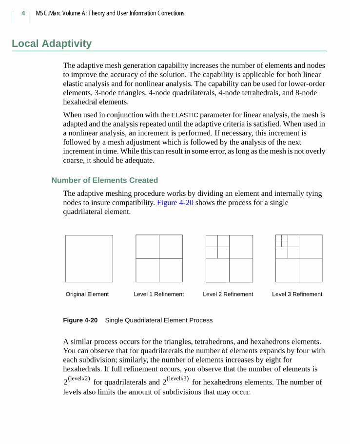
The adaptive meshing procedure works by dividing an element and internally tying nodes to insure compatibility. Figure 4-20 shows the process for a single quadrilateral element.
Figure 4-20 Single Quadrilateral Element Process
A similar process occurs for the triangles, tetrahedrons, and hexahedrons elements. You can observe that for quadrilaterals the number of elements expands by four with each subdivision; similarly, the number of elements increases by eight for hexahedrals. If full refinement occurs, you observe that the number of elements is
for quadrilaterals and for hexahedrons elements. The number of levels also limits the amount of subdivisions that may occur.
Original Element Level 1 Refinement Level 2 Refinement Level 3 Refinement
2levelx2( )
2levelx3( )
Chapter 4 Introduction to Mesh Definition5
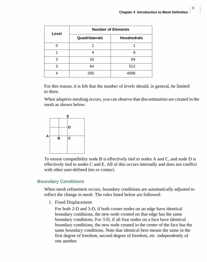
For this reason, it is felt that the number of levels should, in general, be limited to three.
When adaptive meshing occurs, you can observe that discontinuities are created in the mesh as shown below:
To ensure compatibility node B is effectively tied to nodes A and C, and node D is effectively tied to nodes C and E. All of this occurs internally and does not conflict with other user-defined ties or contact.
Boundary Conditions
When mesh refinement occurs, boundary conditions are automatically adjusted to reflect the change in mesh. The rules listed below are followed:
1. Fixed Displacement
For both 2-D and 3-D, if both corner nodes on an edge have identical boundary conditions, the new node created on that edge has the same boundary conditions. For 3-D, if all four nodes on a face have identical boundary conditions, the new node created in the center of the face has the same boundary conditions. Note that identical here means the same in the first degree of freedom, second degree of freedom, etc. independently of one another.
LevelNumber of Elements
Quadrilaterals Hexahedrals
0 1 1
1 4 8
2 16 64
3 64 512
4 256 4096
AB C
D
E

MSC.Marc Volume A: Theory and User Information Corrections
6
2. Point Loads
The point loads remain unchanged on the original node number.
3. Distributed Loads
Distributed loads are automatically placed on the new elements. Caution should be used when using user subroutine FORCEM as the element numbers can be changed due to the new mesh process.
4. Contact
The new nodes generated on the exterior of a body are automatically treated as potential contact nodes. The elements in a deformable body are expanded to include the new elements created. After the new mesh is created, the new nodes are checked to determine if they are in contact.
CAUTION: None of the nodes of an element being subdivided should have a local coordinate system defined through the TRANSFORMATION option.
Location of New Nodes
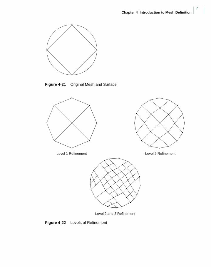
When an element is refined, the default is that the new node on an edge is midside to the two corner nodes. As an alternative, the SURFACE and ATTACH NODE options can be used or user subroutine UCOORD can be used. The SURFACE option can be used to describe the mathematical form of the surface. If the corner nodes of an edge are attached to the surface, the new node is placed upon the actual surface.
This is illustrated in Figure 4-21 and Figure 4-22, where initially a single element is used to represent a circle. The circle is defined with the SURFACE option and the original four nodes are placed on it using the ATTACH NODE option. Notice that the new nodes are placed on the circle.
Chapter 4 Introduction to Mesh Definition7
Figure 4-21 Original Mesh and Surface
Figure 4-22 Levels of Refinement
Level 1 Refinement Level 2 Refinement
Level 2 and 3 Refinement

MSC.Marc Volume A: Theory and User Information Corrections
8
Adaptive Criteria
The adaptive meshing subdivision occurs when a particular adaptive criteria is satisfied. Multiple adaptive criteria can be selected using the ADAPTIVE model definition option. These include:
Mean Strain Energy Criterion
The element is refined if the strain energy of the element is greater than the average strain energy in an element times a given factor, .
(4-31)
Zienkiewicz-Zhu Criterion
The error norm is defined as either
(4-32)
The stress error and strain energy errors are
and (4-33)
where is the smoothed stress and is the calculated stress. Similarly, is for energy.
An element is subdivided if
and
or
and
where NUMEL is the number of elements in the mesh. If , , , and are input
as zero, then .
f1
element strain energytotal strain energy
number of elements----------------------------------------------- * f1>
π2σ∗ σ–( )2
dV∫σ2
dV σ∗ σ–( )2dV∫+∫
--------------------------------------------------------= γ2E∗ E–( )2
dV∫E
2dV E∗ E–( )2
dV∫+∫---------------------------------------------------------=
X σ∗ σ–( )2dV∫= Y E∗ E–( )2
dV∫=
σ* σ E
π f1>
Xel f2 * X/NUMEL f3 * X * f1 π NUMEL⁄⁄+>
γ f1>
Yel f4 * Y/NUMEL f5 * Y * f1 γ NUMEL⁄⁄+>
f2 f3 f4 f5
f2 1.0=

Chapter 4 Introduction to Mesh Definition9
Zienkiewicz – Zhu Plastic Strain Criterion
The plastic strain error norm is defined as .
The plastic strain error is . The allowable element plastic strain
error is . The element will
be subdivided when and . NUMEL is the number of elements in
the mesh.
Zienkiewicz-Zhu Creep Strain Criterion
Zienkiewicz-Zhu creep strain error norm is defined as
. The creep strain error is . The
allowable element creep strain error is
.
The element will be subdivided when and . NUMEL is the number
of elements in the mesh.
Equivalent Values Criterion
This method is based upon either relative or absolute testing using either the equivalent von Mises stress, the equivalent strain, equivalent plastic strain or equivalent creep strain. An element is subdivided if the current element value is a given fraction of the maximum (relative) or above a given absolute value.
or
or
α2εp* εp
–( )2dV∫
εp2dV εp* εp
–( )2dV∫+∫
-----------------------------------------------------------=
A εp* εp–( )
2dV∫=
AEPS f2 * A NUMEL f3 * A * f1 α NUMEL⁄⁄+⁄=
α f1> Ael AEPS>
β2εc* εc
–( )2dV∫
εc2dV εc* εc
–( )2dV∫+∫
----------------------------------------------------------= B εc* εc–( )
2dV∫=
AECS f2 * B NUMEL f3 * B * f1 β NUMEL⁄⁄+⁄=
β f1> Bel AECS>
σvm f1σmax
vm> σvm f2>
εvm f3σmax
vm> εvm f4>
MSC.Marc Volume A: Theory and User Information Corrections
10
Node Within A Box Criterion
An element is subdivided if it falls within the specified box. If all of the nodes of the subdivided elements move outside the box, the elements are merged back together.
Nodes In Contact Criterion
An element is subdivided if one of its nodes is associated with a new contact condition. In the case of a deformable-to-rigid contact, this implies that the node has touched a rigid surface. For deformable-to-deformable contact, the node can be either a tied or retained node. Note that if chattering occurs, there can be an excessive number of elements generated. Use the level option to reduce this problem.
Temperature Gradient Criterion
An element is subdivided if the gradient in the element is greater than a given fraction of the maximum gradient in the solution. This is the recommended method for heat transfer.
User-defined Criterion
User subroutine UADAP can be used to prescribe a user-defined adaptive criteria.
Previously Refined Mesh Criterion
Use the refined mesh from a previous analysis as the starting point to this analysis. The information from the previous adapted analysis is read in.
Chapter 4 Introduction to Mesh Definition11
Global Remeshing
In the analysis of metal or rubber, the materials may be deformed from some initial (maybe simple) shape to a final, very often, complex shape. During the process, the deformation can be so large that the mesh used to model the materials may become highly distorted, and the analysis cannot go any further without using some special techniques. Remeshing/rezoning in Marc is a useful feature to overcome the difficulties.
In the release before MSC.Marc 2000, the global remeshing/rezoning is done manually. When the mesh becomes too distorted because of the large deformation to continue the analysis, the analysis is stopped. A new mesh is created based on the deformed shape of the contact body to be rezoned. A data mapping is performed to transfer necessary data from the old, deformed mesh to the new mesh. The contact tolerance is recalculated (if not specified by you) and the contact conditions are redefined, and the analysis continues.
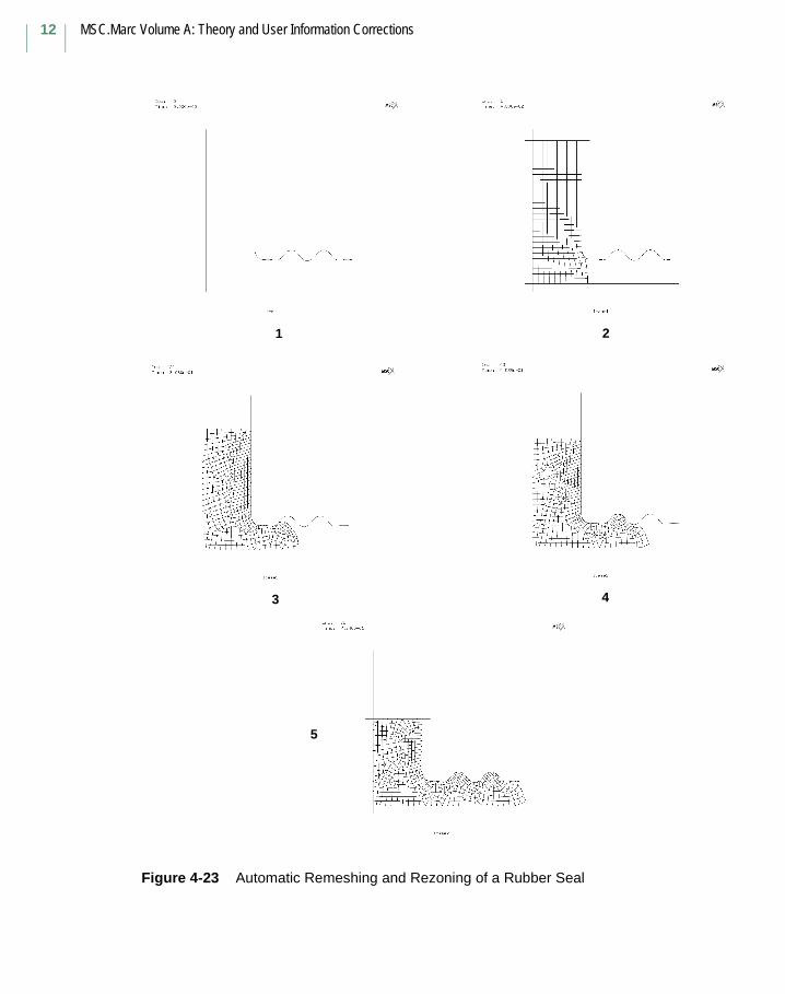
After the release of MSC.Marc 2000, the above steps are done automatically (see Figure 4-23). Based on the different remeshing criteria you specified, the program determines when the remeshing/rezoning is required. The automatic remeshing control can be instructed through the ADAPT GLOBAL option or through automatic time stepping control. With automatic time stepping control, remeshing (if allowed) is forced when the mesh of the body is distorted during the analysis. At the point of remeshing/rezoning on a 2-D application, the program finds the outline of the body to be rezoned and repairs the outline to remove possible penetrations. Then, the program calls the mesher to create a new mesh based on the clean outline. Furthermore, the program performs data transfer from the old mesh to the new mesh, redetermines the contact conditions, and continues the analysis.
The automatic remeshing/rezoning feature can be activated using REZONING,1 parameter. Remeshing/rezoning can be carried out for one or more contact bodies at one increment. Different bodies can use different remeshing/rezoning criteria. The remeshing/rezoning criteria, the bodies to be rezoned, the element target length and other remeshing control parameters for the new meshes are specified by you or by the program via the ADAPT GLOBAL model and history definition options.
Note: Automatic remeshing/rezoning feature only works for two-dimensional cases in the current release of Marc.
Only updated Lagrangian formulation can be used for the feature.
MSC.Marc Volume A: Theory and User Information Corrections
12
Figure 4-23 Automatic Remeshing and Rezoning of a Rubber Seal
1 2
3 4
5
Chapter 4 Introduction to Mesh Definition13
Remeshing Criteria
It is possible to choose any combinations of the following remeshing criteria: Element Distortion, Contact Penetration, Increment, Angle Deviation or Immediate.
Element Distortion
The identified body is remeshed when the distortion in the elements becomes large, or it is anticipated that the distortion will become large.
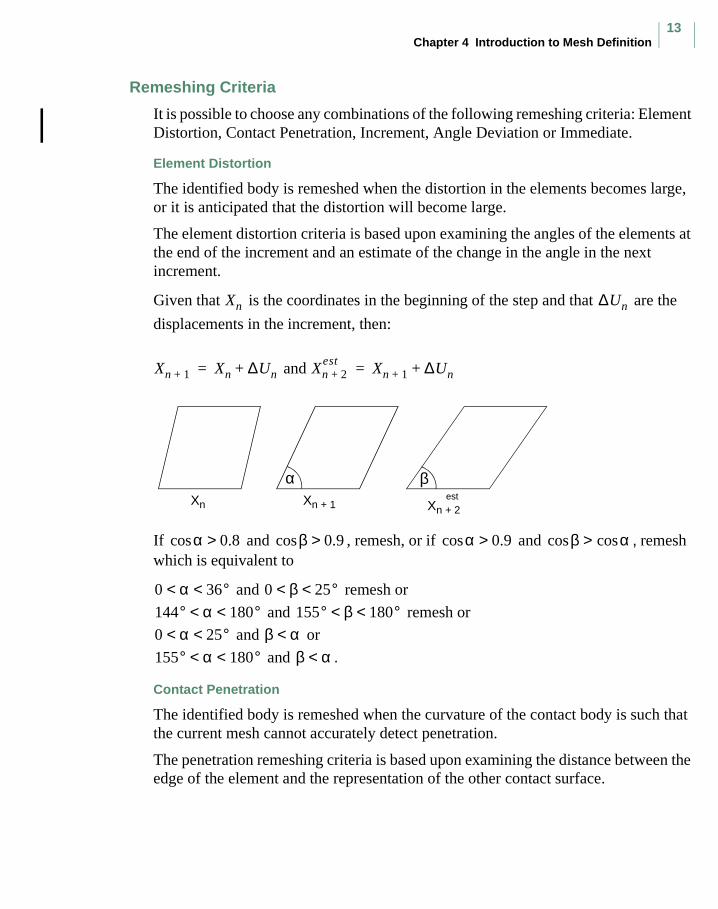
The element distortion criteria is based upon examining the angles of the elements at the end of the increment and an estimate of the change in the angle in the next increment.
Given that is the coordinates in the beginning of the step and that are the
displacements in the increment, then:
and
If and , remesh, or if and , remesh which is equivalent to
and remesh or
and remesh or
and or
and .
Contact Penetration
The identified body is remeshed when the curvature of the contact body is such that the current mesh cannot accurately detect penetration.
The penetration remeshing criteria is based upon examining the distance between the edge of the element and the representation of the other contact surface.
Xn ∆Un
Xn 1+ Xn ∆Un+= Xn 2+est Xn 1+ ∆Un+=
Xn Xn + 1 Xn + 2est
α β
α 0.8>cos β 0.9>cos α 0.9>cos β αcos>cos
0 α 36°< < 0 β 25°< <144° α 180°< < 155° β 180°< <0 α 25°< < β α<155° α 180°< < β α<
MSC.Marc Volume A: Theory and User Information Corrections
14
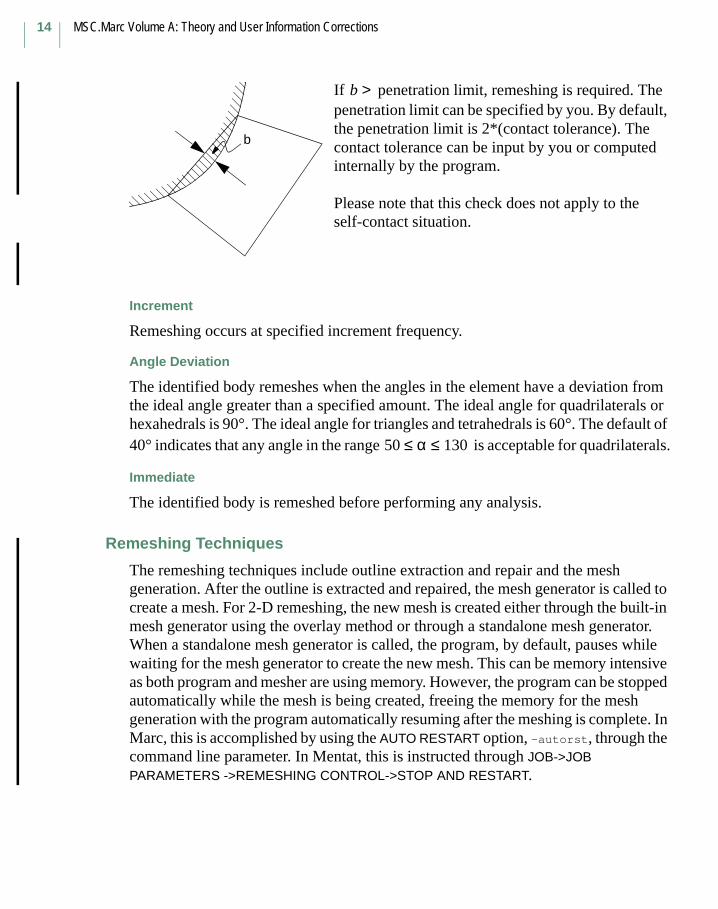
If penetration limit, remeshing is required. The penetration limit can be specified by you. By default, the penetration limit is 2*(contact tolerance). The contact tolerance can be input by you or computed internally by the program.
Please note that this check does not apply to the self-contact situation.
Increment
Remeshing occurs at specified increment frequency.
Angle Deviation
The identified body remeshes when the angles in the element have a deviation from the ideal angle greater than a specified amount. The ideal angle for quadrilaterals or hexahedrals is 90°. The ideal angle for triangles and tetrahedrals is 60°. The default of 40° indicates that any angle in the range is acceptable for quadrilaterals.
Immediate
The identified body is remeshed before performing any analysis.
Remeshing Techniques
The remeshing techniques include outline extraction and repair and the mesh generation. After the outline is extracted and repaired, the mesh generator is called to create a mesh. For 2-D remeshing, the new mesh is created either through the built-in mesh generator using the overlay method or through a standalone mesh generator. When a standalone mesh generator is called, the program, by default, pauses while waiting for the mesh generator to create the new mesh. This can be memory intensive as both program and mesher are using memory. However, the program can be stopped automatically while the mesh is being created, freeing the memory for the mesh generation with the program automatically resuming after the meshing is complete. In Marc, this is accomplished by using the AUTO RESTART option, -autorst, through the command line parameter. In Mentat, this is instructed through JOB->JOB PARAMETERS ->REMESHING CONTROL->STOP AND RESTART.
b
b >
50 α 130≤ ≤
Chapter 4 Introduction to Mesh Definition15
Mesh Generation
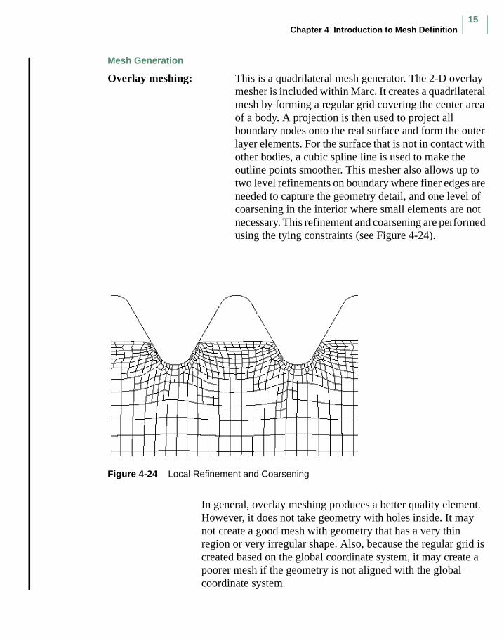
Overlay meshing: This is a quadrilateral mesh generator. The 2-D overlay mesher is included within Marc. It creates a quadrilateral mesh by forming a regular grid covering the center area of a body. A projection is then used to project all boundary nodes onto the real surface and form the outer layer elements. For the surface that is not in contact with other bodies, a cubic spline line is used to make the outline points smoother. This mesher also allows up to two level refinements on boundary where finer edges are needed to capture the geometry detail, and one level of coarsening in the interior where small elements are not necessary. This refinement and coarsening are performed using the tying constraints (see Figure 4-24).
Figure 4-24 Local Refinement and Coarsening
In general, overlay meshing produces a better quality element. However, it does not take geometry with holes inside. It may not create a good mesh with geometry that has a very thin region or very irregular shape. Also, because the regular grid is created based on the global coordinate system, it may create a poorer mesh if the geometry is not aligned with the global coordinate system.
MSC.Marc Volume A: Theory and User Information Corrections
16
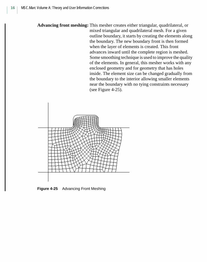
Advancing front meshing: This mesher creates either triangular, quadrilateral, or mixed triangular and quadrilateral mesh. For a given outline boundary, it starts by creating the elements along the boundary. The new boundary front is then formed when the layer of elements is created. This front advances inward until the complete region is meshed. Some smoothing technique is used to improve the quality of the elements. In general, this mesher works with any enclosed geometry and for geometry that has holes inside. The element size can be changed gradually from the boundary to the interior allowing smaller elements near the boundary with no tying constraints necessary (see Figure 4-25).
Figure 4-25 Advancing Front Meshing
Chapter 4 Introduction to Mesh Definition17
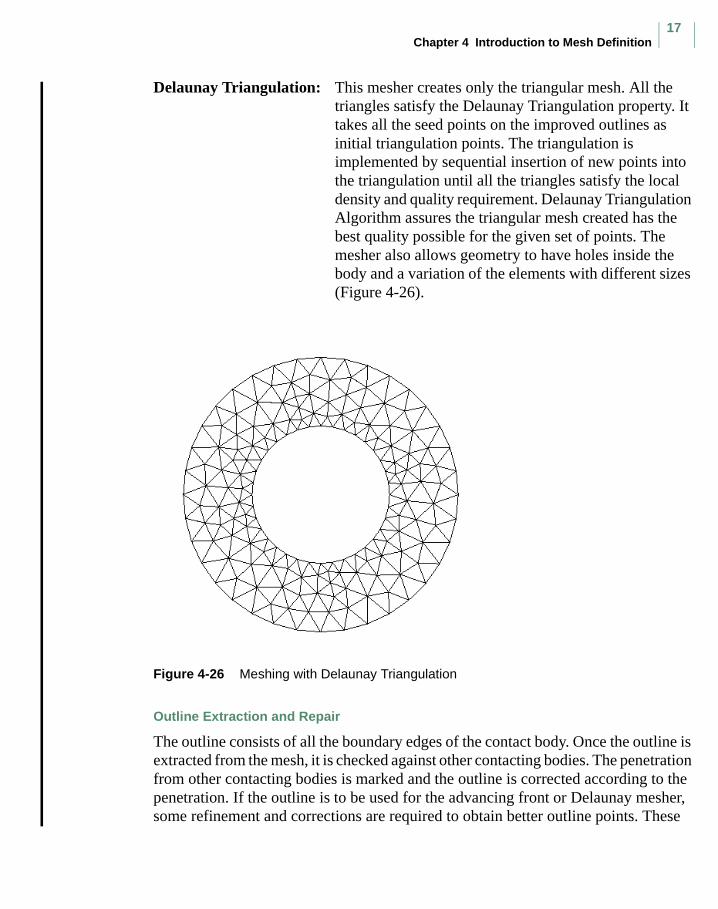
Delaunay Triangulation: This mesher creates only the triangular mesh. All the triangles satisfy the Delaunay Triangulation property. It takes all the seed points on the improved outlines as initial triangulation points. The triangulation is implemented by sequential insertion of new points into the triangulation until all the triangles satisfy the local density and quality requirement. Delaunay Triangulation Algorithm assures the triangular mesh created has the best quality possible for the given set of points. The mesher also allows geometry to have holes inside the body and a variation of the elements with different sizes (Figure 4-26).
Figure 4-26 Meshing with Delaunay Triangulation
Outline Extraction and Repair
The outline consists of all the boundary edges of the contact body. Once the outline is extracted from the mesh, it is checked against other contacting bodies. The penetration from other contacting bodies is marked and the outline is corrected according to the penetration. If the outline is to be used for the advancing front or Delaunay mesher, some refinement and corrections are required to obtain better outline points. These
MSC.Marc Volume A: Theory and User Information Corrections
18
outline points become boundary nodes in the new mesh and cannot be altered during the meshing process. The following procedures are taken by the program to prepare the new outline for the remeshing:
Step 1: Marking the hard points: The hard points are those points that represent important features of the original outline. Hard points are points that mark the beginning of a contact or the last of the contact, and the points that represent a sharp corner (such as 90° angle).
Step 2: Marking the points with target element size and minimum element size: The outline points are placed based on the target element size. The refinements and the user-defined outline points are allowed to change this control. However, the minimum element size is used to make sure the outline segment is not too small for the mesh generation.
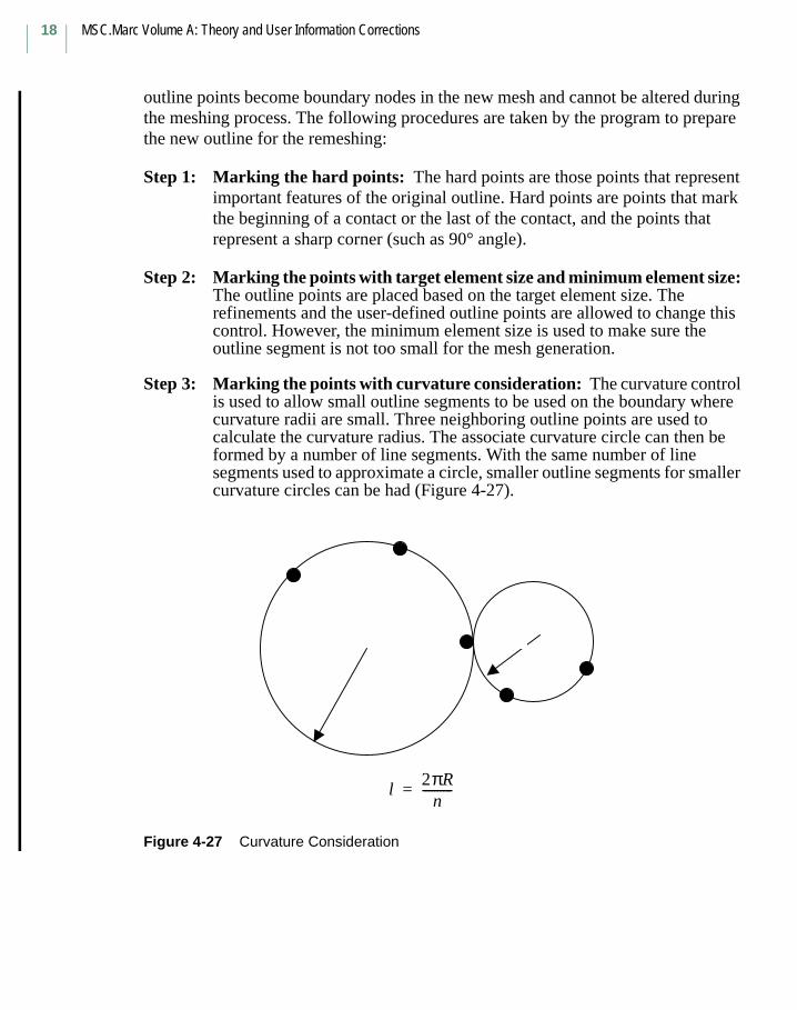
Step 3: Marking the points with curvature consideration: The curvature control is used to allow small outline segments to be used on the boundary where curvature radii are small. Three neighboring outline points are used to calculate the curvature radius. The associate curvature circle can then be formed by a number of line segments. With the same number of line segments used to approximate a circle, smaller outline segments for smaller curvature circles can be had (Figure 4-27).
Figure 4-27 Curvature Consideration
l2πR
n----------=

Chapter 4 Introduction to Mesh Definition19
Step 4: Marking the points with thin region consideration: In the area where a thin region is formed, small elements are preferred. This can be done by detecting the thin region and using smaller outline segments in the area. The segment length used for the thin area is to allow at least three elements to be presented across the thin area.
Step 5: Smoothing the outline points: Smoothing is required on the outline so that the segment length can gradually vary.
Step 6: Interpolations: Interpolation is the actual process to create a new outline based on the extracted outline and the marking of the outline points. Linear interpolation is used on the contact area to prevent penetration into the other contact bodies. Cubic spline line interpolation is used for the free surfaces.
Remeshing Based on the Target Number of Elements
Instead of giving the element size, you can give the target number of elements for the remeshing. The number of elements in the new mesh can also be controlled by using a percentage tolerance to ensure that the new mesh does not have too many or too few elements. However, this tolerance control requires remeshing trials and it cannot be used with automatic stop and restart control.

MSC.Marc Volume A: Theory and User Information Corrections
20
Chapter 5 Structural Procedure
Library

Chapter 5 Structural Procedure Library21
Load Incrementation
Several history definition options are available in Marc to input mechanical and thermal load increments (see Table 5-8). The choice is between a fixed and an automatic load stepping scheme. For a fixed scheme, the load step size remains constant during a load case. The fixed schemes are AUTO LOAD for static mechanical, CREEP INCREMENT for creep, DYNAMIC CHANGE for dynamic mechanical and TRANSIENT NON AUTO for thermal/thermo-mechanically coupled. For an adaptive scheme, the load step size changes from one increment to the other and also within an increment depending on convergence criteria and/or user-defined criteria. The adaptive schemes are AUTO STEP and AUTO INCREMENT for static mechanical, AUTO CREEP and AUTO STEP for creep, AUTO STEP and TRANSIENT for dynamic mechanical and AUTO STEP and TRANSIENT for thermal/thermo-mechanically coupled.
The main automatic scheme is AUTO STEP, which has been greatly enhanced in the 2001 release. Previously, one or more criteria based upon strain, stress displacement, or temperature increments for controlling the time step had to be given. These criteria are still available, but there is a new criterion for automatically controlling the load step based upon the number of recycles. This allows the option to be used directly with default settings for mechanical, thermal and thermomechanically coupled analysis problems. More details on the AUTO STEP scheme are given in the next section.
While the improved AUTO STEP option is designed as the default adaptive stepping procedure, it may still be advantageous to use one of the other available adaptive time-stepping options. This is the case for the following analysis types:
• Post buckling or snap-through analyses requires the so-called arclength method which is available through the AUTO INCREMENT option. This option can only be used in static mechanical analyses and the applied load is automatically increased or decreased in order to maintain a certain arclength. AUTO INCREMENT can also be used for general situations without instabilities, but, in general, the AUTO STEP option is preferred for these situations.
• For creep analysis, the available adaptive options are AUTO CREEP and AUTO STEP. The AUTO CREEP option supports some features which are not available through AUTO STEP (see the description in Volume C). If AUTO STEP is used for creep problems, it may be advisable to use a creep strain increment criterion and a stress increment criterion as additional user-defined criteria in combination with the default recycle criterion. AUTO STEP is usually more reliable in cases involving creep and contact.
• For the case of automatic load stepping for a thermally loaded elastic-creep/elastic-plastic-creep stress analysis, the only available scheme is AUTO THERM CREEP (see Volume C).
MSC.Marc Volume A: Theory and User Information Corrections
22
• For thermally driven mechanical problems, the AUTO THERM option can be used. The thermal loads derived from a thermal analysis are applied using the CHANGE STATE option in a mechanical analysis. The load step of the mechanical analysis is automatically adjusted based upon user-specified (allowed) changes in temperature from the thermal analysis per increment. For example, if there is a change of 50° in the thermal analysis in one increment and you only allowed a change of 10° per increment in the mechanical analysis, AUTO THERM splits up the thermal increment into five mechanical increment.
Selecting Load Increment Size
Selecting a proper load step increment is an important ingredient in a nonlinear solution scheme. Large steps often lead to many recycles per increment and, if the step is too large, it can lead to inaccuracies and non convergence. On the other hand, using too small steps is inefficient.
When a fixed load stepping scheme is used, it is important to select an appropriate load step size that captures the loading history and allows for convergence within a reasonable number of recycles. For complex load histories, it is often necessary to break up the analysis into separate load cases with different step sizes. For fixed stepping, there is an option to have the load step automatically cut back in case of failure to obtain convergence. When an increment diverges, the intermediate deformations after each recycle can show large fluctuations and the final cause of program exit can be any of maximum number of recycles reached (exit 3002), elements going inside out (exit 1005 or 1009) or, in a contact analysis, nodes sliding off a rigid contact body (exit 2400). These deformations are normally not visible as post results (there is a feature to allow for the intermediate results to be available on the post file, see the POST option). If the cut-back feature is activated and one of these
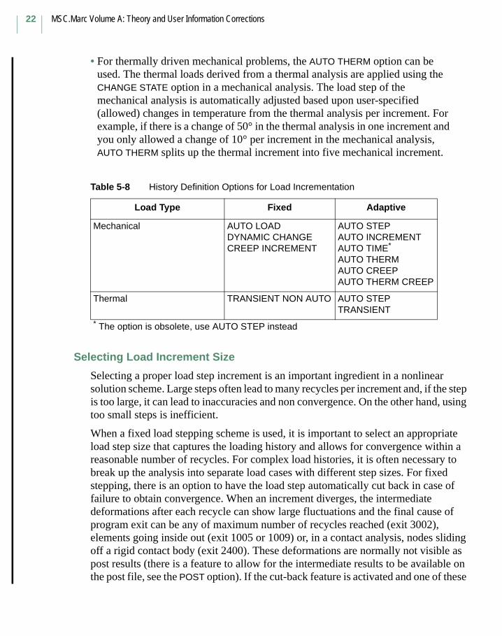
Table 5-8 History Definition Options for Load Incrementation
Load Type Fixed Adaptive
Mechanical AUTO LOADDYNAMIC CHANGECREEP INCREMENT
AUTO STEPAUTO INCREMENTAUTO TIME*
AUTO THERMAUTO CREEPAUTO THERM CREEP
Thermal TRANSIENT NON AUTO AUTO STEPTRANSIENT
* The option is obsolete, use AUTO STEP instead
Chapter 5 Structural Procedure Library23
failures occurs, the state of the analysis at the end of the previous increment is restored from a copy kept in memory, and the increment is subdivided into a number of sub increments. The step size is halved until convergence is obtained or the user-specified number of cut-backs has been performed. Once an increment is converged, the rest of the original increment is completed in equally sized steps unless further cut-backs are necessary. No results are written to the post file during subincrementation, and the original increment count is preserved.
Automatic Load Incrementation
In many nonlinear analyses, it is useful to have Marc figure out the appropriate load step size automatically. The AUTO INCREMENT option is a so-called arc-length method and is designed for applications like post buckling and snap-through analysis. This method is described in detail in Chapter 11, Arc-Length Methods on page 11.
AUTO STEP
The scheme appropriate for most other applications is AUTO STEP. The primary control of the load step is based upon the number of recycles needed to obtained convergence. There are a number of optional user-specified physical criteria that can be used to additionally control the load step. For the recycle based option, the user specifies a desired number of recycles. This number is used as a target value for the load stepping scheme. If the number of recycles needed to obtain convergence exceeds the desired number, the load step size is reduced, the recycle counter is reset to zero and the increment is performed again with the new load step. The factor with which the time step is cut back defaults to 1.2 and can be specified by you. The load step for the next increment is increased if the number of recycles required in the current increment is less than the desired number. The same factor that is used for decreasing the time step is used for increasing it. The load step is never increased during an increment. In addition, the same type of cut-back feature for fixed load stepping is available for this scheme as well. If the maximum number of recycles is reached (exit 3002), elements go inside out (exit 1005/1009), or nodes slide off the end of a rigid contact body (exit 2400), the load step is halved and the increment is redone. Whenever the load step is reduced (either due to number of recycles becoming larger than desired or one of the four exits), the state at the end of the previous increment is restored from a copy kept in memory. This is the principal behavior of the scheme.
There are some exceptions to the basic scheme outlined above. If an increment is consistently converging with the original load step and the number of recycles exceeds the desired number, the number of recycles is allowed to go beyond the
MSC.Marc Volume A: Theory and User Information Corrections
24
desired number until convergence or up to the user specified maximum number. The time step is then decreased for the next increment. An increment is determined to be converging if the convergence ratio was decreasing in three previous recycles.
Special rules also apply in a contact analysis. For quasi-static problems, the AUTO STEP option is designed to only use the automated penetration check option (see CONTACT option, 7th field of 2nd data block; option 3 is always used). Even if you flag the increment splitting penetration check option, Marc internally converts it to automated penetration check. During the recycles, the contact status can keep changing (new nodes come in contact, nodes slide to new segments, separate etc.). Whenever the contact status changes during an increment, a new set of contact constraints are incorporated into the equilibrium equations and more recycles are necessary in order to find equilibrium. These extra recycles, which are solely due to contact changes, are not counted when the comparison is made to the desired number for determining if the load step needs to be decreased within the increment. Thus, only true Newton-Raphson iterations are taken into account. For the load step of the next increment, the accumulated number of recycles during the previous increment is used. This ensures that the time step is not increased when there are many changes in contact during the previous increment.
In addition to allowing Marc to use the number of recycles for automatically controlling the step size for AUTO STEP, user-specified physical criteria can be used for controlling the step size. You can specify the maximum allowed incremental change within certain ranges for specific quantities during an increment. The quantities available are displacements, rotations, stresses, strains, strain energy, and temperature (in thermal or thermomechanically coupled analyses). These criteria can be utilized in two ways. By default, they are used as limits, which means that the load step is decreased if a criterion is violated during the current increment, but they do not influence the decision to change the load step for the next increment (that is, only the actual number of recycles versus desired number of recycles controls the load step for the next increment). The criteria can also be used as targets; in which case, they are used as the main means for controlling the time step for the current and next increments. If the calculated values of the criteria are higher than the user-specified values, the time step is scaled down. If the obtained values for a converged increment are less than the user specified, the time step is scaled up. The scale factor used is the ratio between the actual value and the target value, and this factor is limited by user-specified minimum and maximum factors (defaults to 0.1 and 10 respectively). If this type of load step control is used together with the recycle based control, the time step can be reduced due to whichever criterion that is violated. The decision to increase the step size for the next increment is based upon the physical criteria.
Chapter 5 Structural Procedure Library25
In many analyses, it is convenient to obtain post file results at specified time intervals. This is naturally obtained with a fixed load stepping scheme but not with an automatic
scheme. Traditionally, the post output frequency is given as every nth increment. With the AUTO STEP option, you can request post output to be obtained at equally spaced time intervals. In this case, the time step is temporarily modified to exactly reach the time for output. The time step is then restored in the following increment.
The AUTO STEP option also has an artificial damping feature available for mechanical statics analysis. If the time step is decreased to below the user-specified minimum time step, Marc normally stops with exit number 3015, but if the artificial damping feature is activated, the analysis is continued with a smaller time step. The solution is stabilized by adding a factored mass matrix to the stiffness matrix. This artificial stabilization is turned off once the time step increases above the minimum time step. No post file results are written while the artificial damping is active. The critical parameter for this feature is the (artificial) mass density. You need to specify an appropriate value for all materials in the model.
The defaults of the AUTO STEP scheme are carefully chosen to be adequate in a wide variety of applications. There are cases, however, when the settings may need to be modified. Assume that the default settings are used, which means that the recycle based control is active with an initial load of one per cent of the total. If the structure is weakly nonlinear, convergence can be obtained in just a few recycles even if the step is large. In certain cases this may lead to an inaccurate solution. It can also lead to problems if an initially weakly nonlinear structure suddenly exhibits stronger nonlinearities; for instance, occurrence of plasticity or parts coming into contact. Possible remedies to this problem include:
(i) decrease the time step scale factor from 1.2 to a smaller number so the step size does not grow so rapidly;
(ii) use a physical criterion like maximum increment of displacements to limit the load step;
(iii)use the maximum time step to limit large steps;
(iv)decrease the desired and maximum number of recycles to make the scheme more prone to decrease the load step if more recycles are needed.
Another situation is if the structure is highly nonlinear and convergence is slow. In this case, it may be necessary to increase the desired number and maximum number of recycles. In general, there is a close connection between the convergence tolerances used and the desired number and maximum number of recycles. In many cases, it may be beneficial to use one or more physical criteria; for example, the increment of plastic strain as targets for controlling the load step.
MSC.Marc Volume A: Theory and User Information Corrections
26
Data Transfer from Axisymmetric Analysis to 3-D Analysis
In many cases, it is possible to begin the numerical simulations as a two-dimensional axisymmetric problem even though the final problem is fully three-dimensional. This is advantageous because of the large computational savings. For this to be useful, the first stage of the problem should be truly axisymmetric. The second stage of the problem can be fully three-dimensional. The AXITO3D model definition option is used in the input file of the 3-D problem to transfer results from an axisymmetric analysis into a 3-D analysis. The data from the axisymmetric analysis is stored on the post file. In the 3-D analysis, the results from axisymmetric analysis are used as initial conditions.
There are three steps in performing an axisymmetric to 3-D analysis.
1. Run axisymmetric analysis.
2. Expand axisymmetric model to 3-D model and transfer data from axisymmetric model to 3-D model.
3. Run 3-D analysis.
Most quadrilateral axisymmetric elements (in 3-D case, hexahedral elements), including Herrmann elements, and most available materials, such as metal and rubber, can be used in the axisymmetric to 3-D analysis. For problems involving large deformation, either total or updated Lagrangian formulation must be used. Thermal and dynamic effects are considered.
For more detailed information on this feature, see the model definition option, AXITO3D, in MSC.Marc Volume C: Program Input.

Chapter 6 Nonstructural Procedure Library27
Chapter 6 Nonstructural
Procedure Library
MSC.Marc Volume A: Theory and User Information Corrections
28
Output
Marc prints out both the nodal temperatures and the temperatures at the element centroid when the CENTROID parameter is used, or at the integration points if the ALL POINTS parameter is invoked. You can also indicate on the HEAT parameter for the program to print out the temperature gradients and the resulting nodal fluxes.
To create a file of element and nodal point temperatures, use the POST model definition option. This file can be used as temperature input for performing a thermal stress analysis. This file is processed using the CHANGE STATE option in the subsequent thermal stress analysis. This post file can also interface with Mentat to plot temperature as a function of time.
Heat Transfer with Convection
Marc has the capability to perform heat transfer with convection if the velocity field is known. The numerical solutions of the convection-diffusion equation have been developed in recent years. The streamline-upwind Petro-Galerkin (SUPG) method has been implemented into the Marc heat transfer capability.
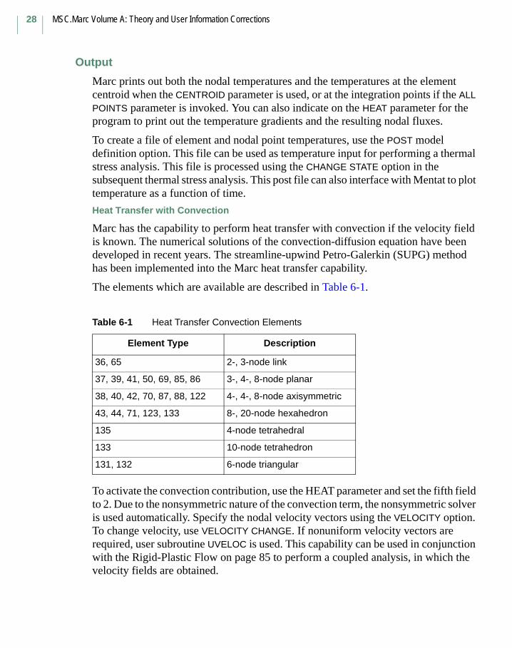
The elements which are available are described in Table 6-1.
To activate the convection contribution, use the HEAT parameter and set the fifth field to 2. Due to the nonsymmetric nature of the convection term, the nonsymmetric solver is used automatically. Specify the nodal velocity vectors using the VELOCITY option. To change velocity, use VELOCITY CHANGE. If nonuniform velocity vectors are required, user subroutine UVELOC is used. This capability can be used in conjunction with the Rigid-Plastic Flow on page 85 to perform a coupled analysis, in which the velocity fields are obtained.
Table 6-1 Heat Transfer Convection Elements
Element Type Description
36, 65 2-, 3-node link
37, 39, 41, 50, 69, 85, 86 3-, 4-, 8-node planar
38, 40, 42, 70, 87, 88, 122 4-, 4-, 8-node axisymmetric
43, 44, 71, 123, 133 8-, 20-node hexahedron
135 4-node tetrahedral
133 10-node tetrahedron
131, 132 6-node triangular
Chapter 6 Nonstructural Procedure Library29
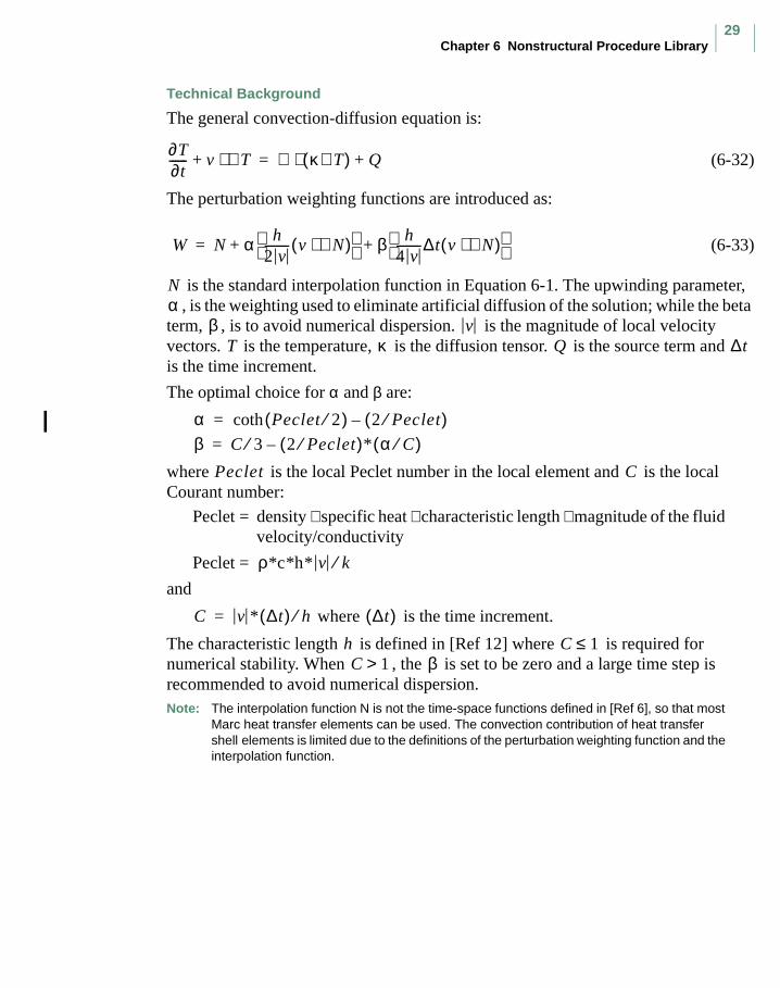
Technical Background
The general convection-diffusion equation is:
(6-32)
The perturbation weighting functions are introduced as:
(6-33)
is the standard interpolation function in Equation 6-1. The upwinding parameter, , is the weighting used to eliminate artificial diffusion of the solution; while the beta
term, , is to avoid numerical dispersion. is the magnitude of local velocity vectors. is the temperature, is the diffusion tensor. is the source term and is the time increment.
The optimal choice for α and β are:
where is the local Peclet number in the local element and is the local Courant number:
Peclet = density ∗ specific heat ∗ characteristic length ∗ magnitude of the fluid velocity/conductivity
Peclet =
and
where is the time increment.
The characteristic length is defined in [Ref 12] where is required for numerical stability. When , the is set to be zero and a large time step is recommended to avoid numerical dispersion.Note: The interpolation function N is not the time-space functions defined in [Ref 6], so that most
Marc heat transfer elements can be used. The convection contribution of heat transfer shell elements is limited due to the definitions of the perturbation weighting function and the interpolation function.
∂T∂t------ v ∇ T⋅+ ∇ κ∇ T( ) Q+⋅=
W N α h2 v-------- v ∇ N⋅( )
β h4 v--------∆t v ∇ N⋅( )
+ +=
Nα
β vT κ Q ∆t
α Peclet 2⁄( ) 2 Peclet⁄( )–coth=
β C 3 2 Peclet⁄( )–⁄ * α C⁄( )=
Peclet C
ρ*c*h* v k⁄
C v * ∆t( ) h⁄= ∆t( )h C 1≤C 1> β
MSC.Marc Volume A: Theory and User Information Corrections
30
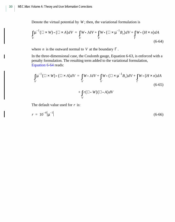
Denote the virtual potential by ; then, the variational formulation is
(6-64)
where is the outward normal to at the boundary .
In the three-dimensional case, the Coulomb gauge, Equation 6-63, is enforced with a penalty formulation. The resulting term added to the variational formulation, Equation 6-64 reads:
(6-65)
The default value used for is:
(6-66)
W
µ 1– ∇ W×( ) ∇ A×( )dV•
V∫ W JdV• W ∇ µ 1–
Br×( )dV• W H n×( )dA•
Γ∫+
V∫+
V∫=
n V Γ
µ 1– ∇ W×( ) ∇ A×( )dV•
V∫ W JdV• W ∇ µ 1–
Br×( )dV• W H n×( )dA•
Γ∫+
V∫+
V∫=
r ∇ W•( ) ∇ A•( ) VdV∫+
r
r 104– µ 1–
=

Chapter 7 Material Library31
Chapter 7 Material Library
MSC.Marc Volume A: Theory and User Information Corrections
32
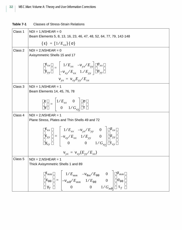
Table 7-1 Classes of Stress-Strain Relations
Class 1 NDI = 1,NSHEAR = 0Beam Elements 5, 8, 13, 16, 23, 46, 47, 48, 52, 64, 77, 79, 142-148
Class 2 NDI = 2,NSHEAR = 0Axisymmetric Shells 15 and 17
Class 3 NDI = 1,NSHEAR = 1Beam Elements 14, 45, 76, 78
Class 4 NDI = 2,NSHEAR = 1Plane Stress, Plates and Thin Shells 49 and 72
Class 5 NDI = 2,NSHEAR = 1Thick Axisymmetric Shells 1 and 89
ε 1 Exx⁄ σ [=
εxx
εyy 1 Exx⁄ νyx Eyy⁄–
νxy Exx⁄– 1. Eyy⁄
σxx
σyy
=
νyx νxyEyy Exx⁄=
εγ
1 Exx⁄ 0
0 1 Gxy⁄
στ
=
εxx
εyy
γxy
1 Exx⁄ νyx Eyy⁄– 0
νxy Exx⁄– 1 Eyy⁄ 0
0 0 1 Gxy⁄
σxx
σyy
τxy
=
νyx νxy Eyy Exx⁄( )=
εmm
εθθ
γT 1 Emm⁄ νθm Eθθ⁄– 0
νmθ Emm⁄– 1 Eθθ⁄ 0
0 0 1 Gmθ⁄
σmm
σθθ
τT
=
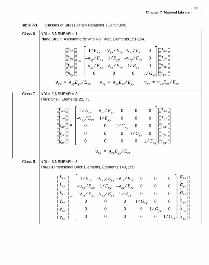
Chapter 7 Material Library33
Class 6 NDI = 3,NSHEAR = 1Plane Strain, Axisymmetric with No Twist, Elements 151-154.
Class 7 NDI = 2,NSHEAR = 3Thick Shell, Elements 22, 75
Class 8 NDI = 3,NSHEAR = 3Three-Dimensional Brick Elements, Elements 149, 150
Table 7-1 Classes of Stress-Strain Relations (Continued)
εxx
εyy
εzz
γxy 1 Exx⁄ νyx Eyy⁄– νzx Ezz⁄– 0
νxy Exx⁄– 1 Eyy⁄ νzy Ezz⁄– 0
νxz Exx⁄– νyz Eyy⁄– 1 Ezz⁄ 0
0 0 0 1 Gxy⁄
σxx
σyy
σzz
τzx
=
νyx νxyEyy Exx⁄= νzy νyzEzz Eyy⁄= νxz νzxExx Ezz⁄=
εxx
εyy
γxy
γyz
γzx 1 Exx⁄ νyx Eyy⁄– 0 0 0
νxy Exx⁄– 1 Eyy⁄ 0 0 0
0 0 1 Gxy⁄ 0 0
0 0 0 1 Gyz⁄ 0
0 0 0 0 1 Gzx⁄
σxx
σyy
τxy
τyz
τxy
=
νxy νxyEyy Exx⁄=
εxx
εyy
εzz
γxy
γyz
γzx 1 Exx⁄ νyx Eyy⁄– νzx Ezz⁄– 0 0 0
νxy Exx⁄– 1 Eyy⁄ νzy Ezz⁄– 0 0 0
νxz Exx⁄– νyz Eyy⁄– 1. Ezz⁄ 0 0 0
0 0 0 1 Gxy⁄ 0 0
0 0 0 0 1 Gyz⁄ 0
0 0 0 0 0 1 Gzx⁄
σxx
σyy
σzz
τxy
τyz
τzx
=

MSC.Marc Volume A: Theory and User Information Corrections
34
Mohr-Coulomb Material (Hydrostatic Yield Dependence)
Marc includes options for elastic-plastic behavior based on a yield surface that exhibits hydrostatic stress dependence. Such behavior is observed in a wide class of soil and rock-like materials. These materials are generally classified as Mohr-Coulomb materials (generalized von Mises materials). Ice is also thought to be a Mohr-Coulomb material. The generalized Mohr-Coulomb model developed by Drucker and Prager is implemented in Marc. There are two types of Mohr-Coulomb materials: linear and parabolic. Each is discussed on the following pages.
Linear Mohr-Coulomb Material
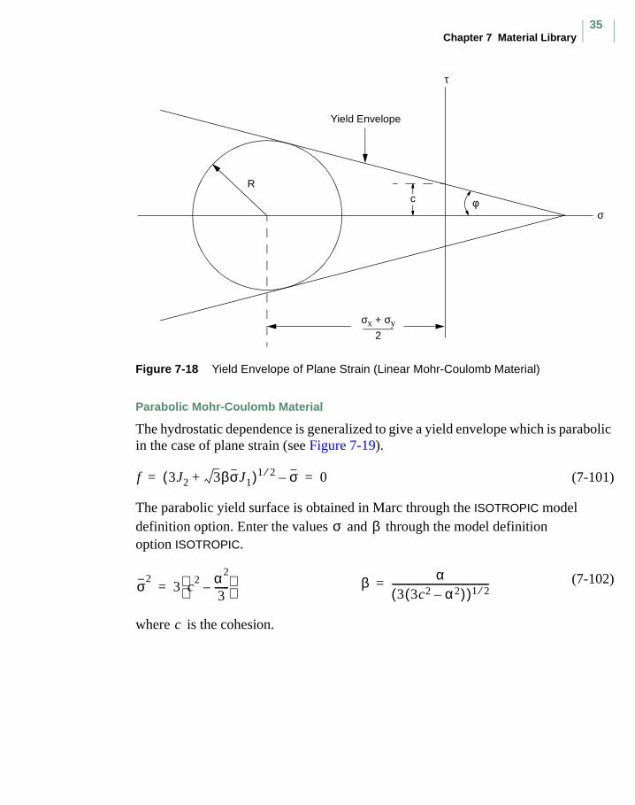
The deviatoric yield function, as shown in Figure 7-18, is assumed to be a linear function of the hydrostatic stress.
(7-97)
where
(7-98)
(7-99)
Analysis of linear Mohr-Coulomb material based on the constitutive description above is available in Marc through the ISOTROPIC model definition option. Through the ISOTROPIC option, the values of and are entered. Note that, throughout the program, the convention that the tensile direct stress is positive is maintained, contrary to its use in many soil mechanics texts.
The constants and can be related to and by
(7-100)
where is the cohesion and is the angle of friction.
f αJ1 J21 2⁄ σ
3-------–+ 0= =
J1 σii=
J212---σ′
ijσ′
ij=
σ α
α σ c φ
cσ
3 1 12α2–( )[ ] 1 2⁄------------------------------------------ 3α
1 3α2–( )1 2⁄-------------------------------; φsin= =
c φ
Chapter 7 Material Library35
Figure 7-18 Yield Envelope of Plane Strain (Linear Mohr-Coulomb Material)
Parabolic Mohr-Coulomb Material
The hydrostatic dependence is generalized to give a yield envelope which is parabolic in the case of plane strain (see Figure 7-19).
(7-101)
The parabolic yield surface is obtained in Marc through the ISOTROPIC model definition option. Enter the values and through the model definition option ISOTROPIC.
(7-102)
where is the cohesion.
Yield Envelope
c
σφ
R
σx + σy2
τ
f 3J2 3βσJ1+( )1 2⁄ σ– 0= =
σ β
β α3 3c2 α2–( )( )1 2⁄-----------------------------------------=σ2
3 c2 α2
3------–
=
c
MSC.Marc Volume A: Theory and User Information Corrections
36
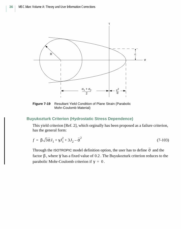
Figure 7-19 Resultant Yield Condition of Plane Strain (Parabolic Mohr-Coulomb Material)
Buyukozturk Criterion (Hydrostatic Stress Dependence)
This yield criterion [Ref. 2], which orginally has been proposed as a failure criterion, has the general form:
(7-103)
Through the ISOTROPIC model definition option, the user has to define and the
factor , where has a fixed value of . The Buyukozturk criterion reduces to the
parabolic Mohr-Coulomb criterion if .
c2
c
σ
R
σx + σy2 α
τ
f β 3σJ1 γJ12
3J2 σ2–+ +=
σβ γ 0.2
γ 0=

Chapter 7 Material Library37
Damage Models
In many structural applications, the finite element method is used to predict failure. This is often performed by comparing the calculated solution to some failure criteria, or by using classical fracture mechanics. Previously, we discussed two models where the actual material model changed due to some failure, see Progressive Composite Failure on page 22 and the previous section on Low Tension Material on page 100. In this section, the damage models appropriate for ductile metals and elastomeric materials will be discussed.
Ductile Metals
In ductile materials given the appropriate loading conditions, voids will form in the material, grow, then coalesce, leading to crack formation and potentially, failure. Experimental studies have shown that these processes are strongly influenced by hydrostatic stress. Gurson studied microscopic voids in materials and derived a set of modified constitutive equations for elastic-plastic materials. Tvergaard and Needleman modified the model with respect to the behavior for small void volume fractions and for void coalescence.
In the modified Gurson model, the amount of damage is indicated with a scalar parameter called the void volume fraction f. The yield criterion for the macroscopic assembly of voids and matrix material is given by:
(7-233)
as seen in Figure 7-53.
The parameter was introduced by Tvergaard to improve the Gurson model at
small values of the void volume fraction. For solids with periodically spaced voids, numerical studies [10] showed that the values of and were
quite accurate.
Fσσy-----
22q1f∗
q2σkk
2σy-------------
1 q1f∗( )2+[ ]–cosh+ 0= =
q1
q1 1.5= q2 1=

MSC.Marc Volume A: Theory and User Information Corrections
38
Chapter 8 Contact

Chapter 8 Contact39
Numbering of Contact Bodies
When defining contact bodies for a deformable-to-deformable analysis, it is important to define them in the proper order. As a general rule, a body with a finer mesh should be defined before a body with a coarser mesh.
Note: For problems involving adaptive meshing or automated remeshing, care must be taken to satisfy this rule before as well as after the mesh change.
If one has defined a body numbering which violates the general rule, or if the rule is violated upon remeshing, then a CONTACT TABLE model or history definition option can be used to modify the order in which contact will be established. This order can be directly user-defined or decided by the program. In the latter case, the order is based on the rule that if two deformable bodies might come into contact, searching is done for nodes of the body having the smallest element edge length. It should be noted that this implies single-sided contact for this body combination, as opposed to the default double-sided contact.
MSC.Marc Volume A: Theory and User Information Corrections
40
Automatic Penetration Checking Procedure
To detect contact between bodies whose boundaries are moving towards each other, an automatic penetration checking procedure is available. This procedure significantly increases accuracy and stability for models in which boundary nodes are displacing significantly. Typical examples include metal forming processes (sheet forming and forging), highly deformable elastomeric models (rubber boots), and snap-fit problems (inserting a key into a lock).
The automatic penetration checking procedure is available under the CONTACT option. It is automatically activated if the adaptive loading procedure is selected. It is not currently available for dynamics or the arc length control procedure. If the automatic penetration checking procedure is selected for these two options, a different procedure, as described below, is used instead.
From a computational perspective, the automatic penetration checking procedure detects penetration each time displacements are updated.
For implicit analysis, this typically happens after a matrix solution which produces a change in the displacements due to a change in applied loads and internal forces. The procedure detects nodes traversing a contact boundary due to the change in displacements. If at least one node penetrates a contact surface, a scale factor is applied to the change in displacements such that the penetrating nodes are moved back to the contact surface.
The automatic penetration checking procedure can, therefore, be considered to be a type of a line search. The procedure also looks at the magnitude of the change in displacement of nodes which already are contacting and not necessarily penetrating. Using stability considerations, the scale factor calculated above may be further modified. In addition, for nodes on a contact boundary which are not yet contacting, a similar procedure is followed to enhance stability.
Because the procedure can reduce the change in displacements, it may require more iterations to complete an increment. It is important to ensure that the maximum allowable number of iterations to complete an increment is set to a sufficiently large value. When the adaptive loading procedure is used, or when the fixed time stepping procedure is used with automatic restarting, the increment automatically restarts if the maximum allowable number of iterations is exceeded. In the case of the adaptive loading procedure, the time step is modified.
When dynamics or the arc length control method is used, the above procedure is not available. Instead, penetration is checked for when convergence is achieved, usually after multiple iterations.

Chapter 9 Boundary Conditions41
Chapter 9 Boundary Conditions
MSC.Marc Volume A: Theory and User Information Corrections
42
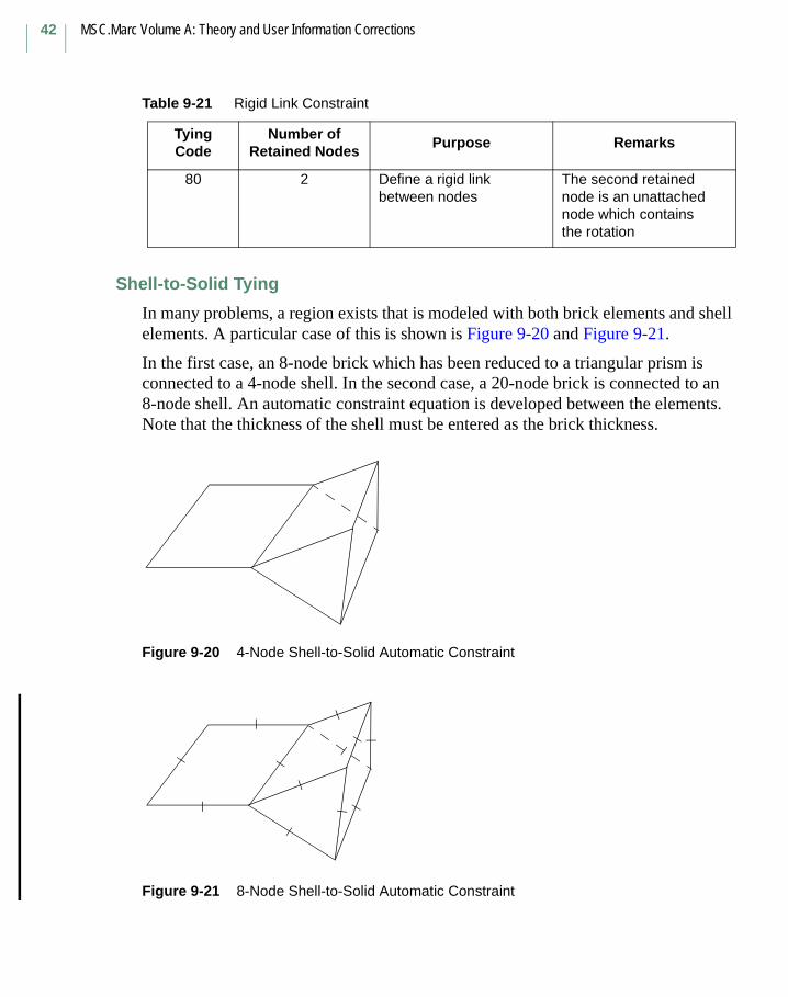
Shell-to-Solid Tying
In many problems, a region exists that is modeled with both brick elements and shell elements. A particular case of this is shown is Figure 9-20 and Figure 9-21.
In the first case, an 8-node brick which has been reduced to a triangular prism is connected to a 4-node shell. In the second case, a 20-node brick is connected to an 8-node shell. An automatic constraint equation is developed between the elements. Note that the thickness of the shell must be entered as the brick thickness.
Figure 9-20 4-Node Shell-to-Solid Automatic Constraint
Figure 9-21 8-Node Shell-to-Solid Automatic Constraint
Table 9-21 Rigid Link Constraint
Tying Code
Number of Retained Nodes
Purpose Remarks
80 2 Define a rigid link between nodes
The second retained node is an unattached node which contains the rotation
Chapter 9 Boundary Conditions43
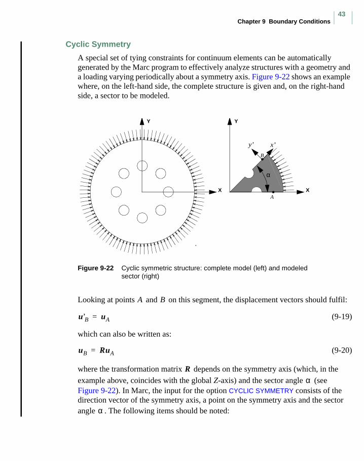
Cyclic Symmetry
A special set of tying constraints for continuum elements can be automatically generated by the Marc program to effectively analyze structures with a geometry and a loading varying periodically about a symmetry axis. Figure 9-22 shows an example where, on the left-hand side, the complete structure is given and, on the right-hand side, a sector to be modeled.
Figure 9-22 Cyclic symmetric structure: complete model (left) and modeled sector (right)
Looking at points and on this segment, the displacement vectors should fulfil:
(9-19)
which can also be written as:
(9-20)
where the transformation matrix depends on the symmetry axis (which, in the
example above, coincides with the global Z-axis) and the sector angle (see Figure 9-22). In Marc, the input for the option CYCLIC SYMMETRY consists of the direction vector of the symmetry axis, a point on the symmetry axis and the sector angle . The following items should be noted:
X
Y
X
Y
x’y’
A
B
α
A B
u’B uA=
uB RuA=
Rα
α
MSC.Marc Volume A: Theory and User Information Corrections
44
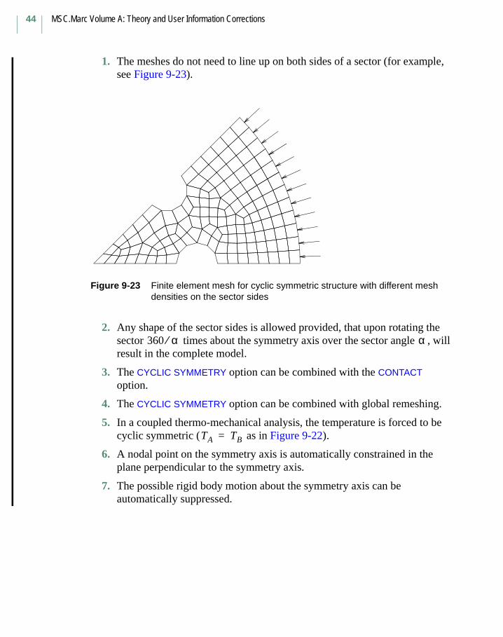
1. The meshes do not need to line up on both sides of a sector (for example, see Figure 9-23).
Figure 9-23 Finite element mesh for cyclic symmetric structure with different mesh densities on the sector sides
2. Any shape of the sector sides is allowed provided, that upon rotating the sector times about the symmetry axis over the sector angle , will result in the complete model.
3. The CYCLIC SYMMETRY option can be combined with the CONTACT option.
4. The CYCLIC SYMMETRY option can be combined with global remeshing.
5. In a coupled thermo-mechanical analysis, the temperature is forced to be cyclic symmetric ( as in Figure 9-22).
6. A nodal point on the symmetry axis is automatically constrained in the plane perpendicular to the symmetry axis.
7. The possible rigid body motion about the symmetry axis can be automatically suppressed.
360 α⁄ α
TA TB=
Chapter 9 Boundary Conditions45
Cross Section
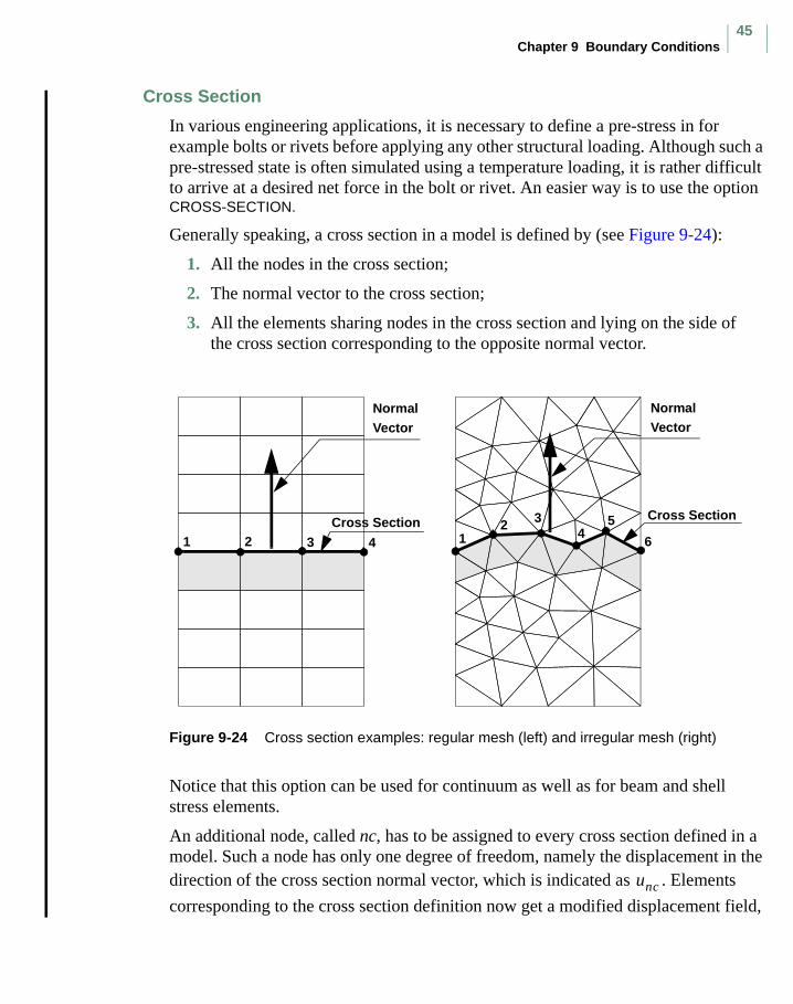
In various engineering applications, it is necessary to define a pre-stress in for example bolts or rivets before applying any other structural loading. Although such a pre-stressed state is often simulated using a temperature loading, it is rather difficult to arrive at a desired net force in the bolt or rivet. An easier way is to use the option CROSS-SECTION.
Generally speaking, a cross section in a model is defined by (see Figure 9-24):
1. All the nodes in the cross section;
2. The normal vector to the cross section;
3. All the elements sharing nodes in the cross section and lying on the side of the cross section corresponding to the opposite normal vector.
Figure 9-24 Cross section examples: regular mesh (left) and irregular mesh (right)
Notice that this option can be used for continuum as well as for beam and shell stress elements.
An additional node, called nc, has to be assigned to every cross section defined in a model. Such a node has only one degree of freedom, namely the displacement in the direction of the cross section normal vector, which is indicated as . Elements
corresponding to the cross section definition now get a modified displacement field,
1 2 3 4 12 3
45
6
Normal Normal
Cross Section Cross Section
Vector Vector
unc
MSC.Marc Volume A: Theory and User Information Corrections
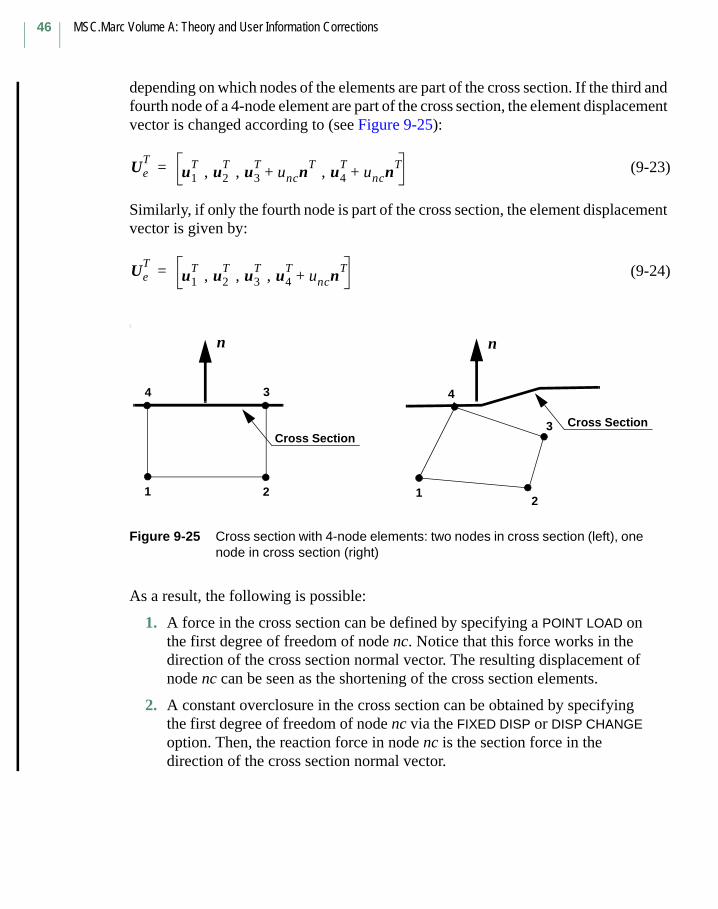
46
depending on which nodes of the elements are part of the cross section. If the third and fourth node of a 4-node element are part of the cross section, the element displacement vector is changed according to (see Figure 9-25):
(9-23)
Similarly, if only the fourth node is part of the cross section, the element displacement vector is given by:
(9-24)
:
Figure 9-25 Cross section with 4-node elements: two nodes in cross section (left), one node in cross section (right)
As a result, the following is possible:
1. A force in the cross section can be defined by specifying a POINT LOAD on the first degree of freedom of node nc. Notice that this force works in the direction of the cross section normal vector. The resulting displacement of node nc can be seen as the shortening of the cross section elements.
2. A constant overclosure in the cross section can be obtained by specifying the first degree of freedom of node nc via the FIXED DISP or DISP CHANGE option. Then, the reaction force in node nc is the section force in the direction of the cross section normal vector.
UeT
u1T
, u2T
, u3T
uncnT+ , u4
TuncnT
+=
UeT
u1T
, u2T
, u3T
, u4T
uncnT+=
1
Cross Section
4 3
2
n
1
Cross Section
4
3
2
n

Chapter 9 Boundary Conditions47
During an analysis, you can switch from one of the above options to the other. So, to simulate the behavior of a pre-stressed bolt under additional loading conditions, you should first define the pre-tension force via the POINT LOAD option and subsequently use the DISP CHANGE option to "lock" the bolt by setting the incremental displacement to zero.
If you are only interested in the total force in the cross section, the displacement
should be set to zero. Then, the total force in the cross section is given by the reaction force in node nc.
∆unc
unc

MSC.Marc Volume A: Theory and User Information Corrections
48
Chapter 10 Element Library
Chapter 10 Element Library49
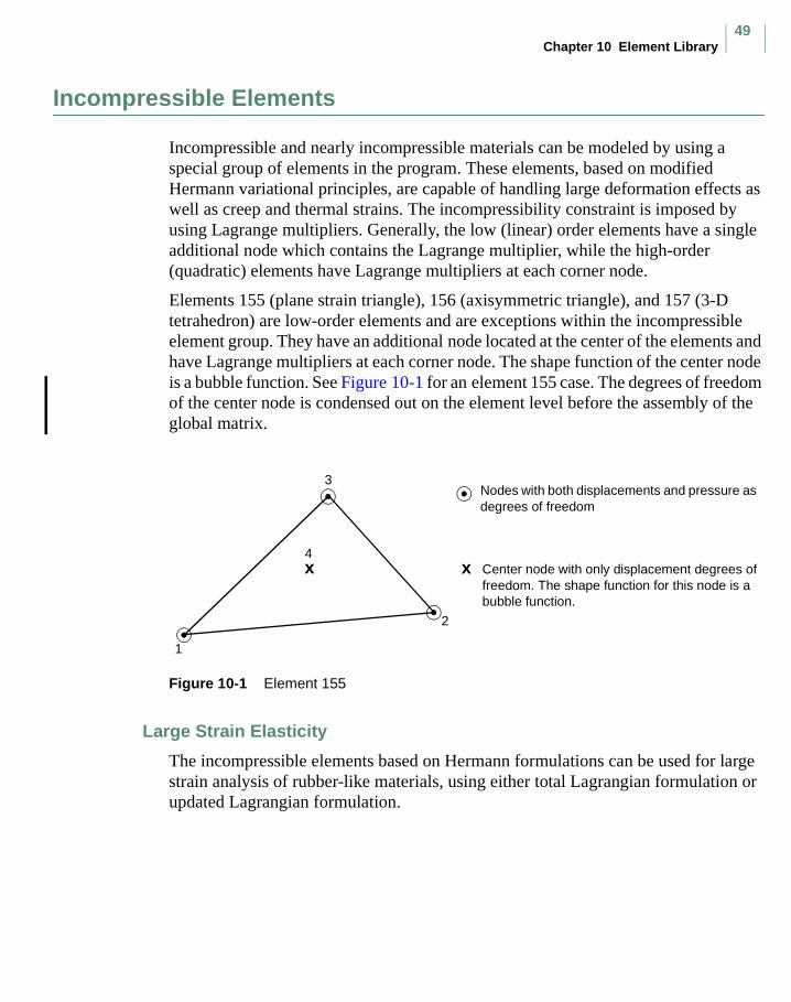
Incompressible Elements
Incompressible and nearly incompressible materials can be modeled by using a special group of elements in the program. These elements, based on modified Hermann variational principles, are capable of handling large deformation effects as well as creep and thermal strains. The incompressibility constraint is imposed by using Lagrange multipliers. Generally, the low (linear) order elements have a single additional node which contains the Lagrange multiplier, while the high-order (quadratic) elements have Lagrange multipliers at each corner node.
Elements 155 (plane strain triangle), 156 (axisymmetric triangle), and 157 (3-D tetrahedron) are low-order elements and are exceptions within the incompressible element group. They have an additional node located at the center of the elements and have Lagrange multipliers at each corner node. The shape function of the center node is a bubble function. See Figure 10-1 for an element 155 case. The degrees of freedom of the center node is condensed out on the element level before the assembly of the global matrix.
Figure 10-1 Element 155
Large Strain Elasticity
The incompressible elements based on Hermann formulations can be used for large strain analysis of rubber-like materials, using either total Lagrangian formulation or updated Lagrangian formulation.
x
1
2
3
4
Nodes with both displacements and pressure as degrees of freedom
Center node with only displacement degrees of freedom. The shape function for this node is a bubble function.
x

MSC.Marc Volume A: Theory and User Information Corrections
50
Chapter 11 Solution Procedures for
Nonlinear Systems

Chapter 11 Solution Procedures for Nonlinear Systems51
Convergence Controls
The default procedure for convergence criterion in Marc is based on the magnitude of the maximum residual load compared to the maximum reaction force. This method is appropriate since the residuals measure the out-of-equilibrium force, which should be minimized. This technique is also appropriate for Newton methods, where zero-load iterations reduce the residual load. The method has the additional benefit that convergence can be satisfied without iteration.
The basic procedures are outlined below.
1. RESIDUAL CHECKING
(11-44)
(11-45)
(11-46)
(11-47)
Where is the force vector, and is the moment vector. and
are control tolerances. indicates the component of with the
highest absolute value. Residual checking has two drawbacks. First, if the CENTROID parameter is used, the residuals and reactions are not calculated accurately. Second, in some special problems, such as free thermal expansion, there are no reaction forces. The program uses displacement checking in either of these cases.
2. DISPLACEMENT CHECKING
(11-48)
(11-49)
(11-50)
(11-51)
Fresidual ∞Freaction ∞
---------------------------- TOL1<
Fresidual ∞Freaction ∞
---------------------------- TOL1 and<Mresidual ∞Mreaction ∞
------------------------------ TOL2<
Fresidual ∞ TOL1<
Fresidual ∞ TOL1 and Mresidual ∞ TOL2<<
F M TOL1
TOL2 F ∞ F
δu ∞∆u ∞
--------------- TOL1<
δu ∞∆u ∞
--------------- TOL1 and<δφ ∞∆φ ∞
--------------- TOL2<
δu ∞ TOL1<
δu ∞ TOL1 and δφ ∞ TOL2<<
MSC.Marc Volume A: Theory and User Information Corrections
52
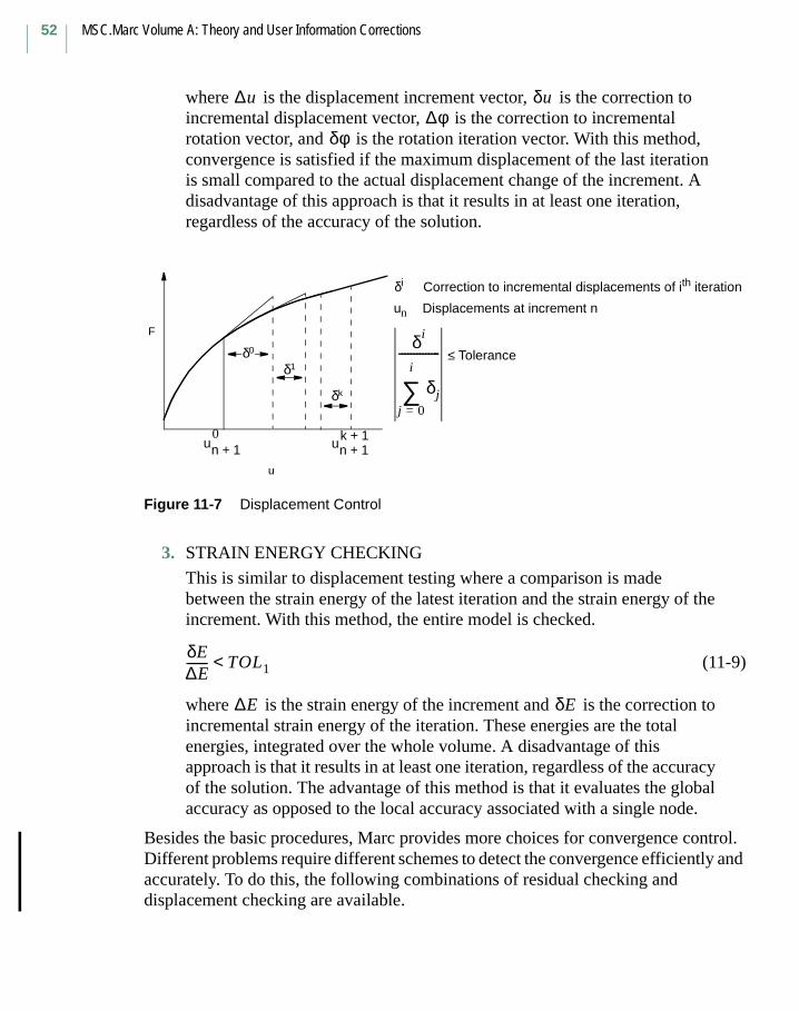
where is the displacement increment vector, is the correction to incremental displacement vector, is the correction to incremental rotation vector, and is the rotation iteration vector. With this method, convergence is satisfied if the maximum displacement of the last iteration is small compared to the actual displacement change of the increment. A disadvantage of this approach is that it results in at least one iteration, regardless of the accuracy of the solution.
Figure 11-7 Displacement Control
3. STRAIN ENERGY CHECKING
This is similar to displacement testing where a comparison is made between the strain energy of the latest iteration and the strain energy of the increment. With this method, the entire model is checked.
(11-9)
where is the strain energy of the increment and is the correction to incremental strain energy of the iteration. These energies are the total energies, integrated over the whole volume. A disadvantage of this approach is that it results in at least one iteration, regardless of the accuracy of the solution. The advantage of this method is that it evaluates the global accuracy as opposed to the local accuracy associated with a single node.
Besides the basic procedures, Marc provides more choices for convergence control. Different problems require different schemes to detect the convergence efficiently and accurately. To do this, the following combinations of residual checking and displacement checking are available.
∆u δu∆φ
δφ
F
u
δk
δ1δ0
Correction to incremental displacements of ith iterationδi
Displacements at increment nun
δi
δjj 0=
i
∑-------------- ≤ Tolerance
un 1+0
un 1+k 1+
δE∆E------- TOL1<
∆E δE

Chapter 11 Solution Procedures for Nonlinear Systems53
4. RESIDUAL OR DISPLACEMENT CHECKING
This procedure does convergence checking on both residuals (Procedure 1) and displacements (Procedure 2). Convergence is obtained if one converges.
5. RESIDUAL AND DISPLACEMENT CHECKING
This procedure does a convergence check on both residuals and displacements (Procedure 4). Convergence is achieved if both criteria converge simultaneously.
For problems where maximum reactions or displacements are extremely small (even close to the round-off errors of computers), the convergence check based on relative values could be meaningless if the convergence criteria chosen is based on these small values. It is necessary to check the convergence with absolute values; otherwise, the analysis is prematurely terminated due to a nonconvergent solution. Such situations are not predicable and usually happen at certain stages of an analysis. For example, problems with stress free motion (rigid body motion or free thermal expansion) and small displacements (springback or constraint thermal expansion) may need to check absolute value at some stage of the analysis. However, it is not convenient and it is also difficult to determine when to check the absolute value and how small the absolute criterion value should be used due to its unpredictability. In order to reduce human interventions and improve the robustness of an FE analysis, Marc allows you to use the AUTO SWITCH option to switch the convergence check scheme if the above mentioned situation occurs during an FE analysis. Turning ON the AUTO SWITCH option allows Marc to automatically change the convergence check scheme to Procedure 4 if small reactions or displacements are detected. This function can be deactivated by turning the AUTO SWITCH option OFF or specifying an absolute value check.
MSC.Marc Volume A: Theory and User Information Corrections
54
Solution of Linear Equations
The finite element formulation leads to a set of linear equations. The solution is obtained through numerically inverting the system. Because of the wide range of problems encountered with Marc, there are several solution procedures available.
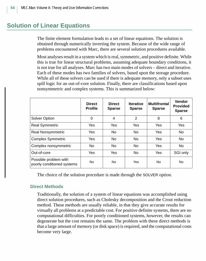
Most analyses result in a system which is real, symmetric, and positive definite. While this is true for linear structural problems, assuming adequate boundary conditions, it is not true for all analyses. Marc has two main modes of solvers – direct and iterative. Each of these modes has two families of solvers, based upon the storage procedure. While all of these solvers can be used if there is adequate memory, only a subset uses spill logic for an out-of-core solution. Finally, there are classifications based upon nonsymmetric and complex systems. This is summarized below:
The choice of the solution procedure is made through the SOLVER option.
Direct Methods
Traditionally, the solution of a system of linear equations was accomplished using direct solution procedures, such as Cholesky decomposition and the Crout reduction method. These methods are usually reliable, in that they give accurate results for virtually all problems at a predictable cost. For positive definite systems, there are no computational difficulties. For poorly conditioned systems, however, the results can degenerate but the cost remains the same. The problem with these direct methods is that a large amount of memory (or disk space) is required, and the computational costs become very large.
Direct Profile
Direct Sparse
Iterative Sparse
Multifrontal Sparse
Vendor Provided Sparse
Solver Option 0 4 2 8 6
Real Symmetric Yes Yes Yes Yes Yes
Real Nonsymmetric Yes No No Yes No
Complex Symmetric Yes No No Yes No
Complex nonsymmetric No No No Yes No
Out-of-core Yes Yes No Yes SGI only
Possible problem with poorly conditioned systems
No No Yes No No
Chapter 11 Solution Procedures for Nonlinear Systems55
Nonsymmetric Systems
The following analyses types result in nonsymmetric systems of equations:
Inclusion of convective terms in heat transfer analysisCoriolis effects in transient dynamic analysisFluid mechanicsSoil analysisFollower force stiffnessFrictional contact
The first three always result in a nonsymmetric system. The last three can be solved either fully using the nonsymmetric solver, or (approximately) using a symmetric solver. The nonsymmetric problem uses twice as much memory for storing the stiffness matrix.
Complex Systems
Marc utilizes a complex operator matrix for dynamic harmonic analyses when the damping matrix is present or for transient electromagnetic analyses. The matrix is always symmetric.
Iterative Solvers
In Marc, an iterative sparse solver is available using a sparse matrix technique. This method is advantageous for different classes of problems.
There exist certain types of analyses for which the sparse iterative solver is not appropriate. These types include:
elastic analysisexplicit creep analysiscomplex harmonic analysissubstructurescentral difference techniqueseigenvalue analysisuse of gap elements
Elastic or explicit creep analysis involves repeated solutions using different load vectors. When a direct solver is used, this is performed very efficiently using back substitution. However, when an iterative solver is used, the stiffness matrix is never inverted, and the solution associated with a new load vector requires a complete re-solution.
The sparse iterative solver can exhibit poor convergence when Herrmann incompressible elements are present.

MSC.Marc Volume A: Theory and User Information Corrections
56
Chapter 12 Output Results

Chapter 12 Output Results57
Status File
The status file contains summarized information of the analysis. Each line within the main content of this file includes the number of load cases and increments; the total cycles, separations from contact surfaces, and cutbacks numbers occurring within each increment; the accumulated total cycles, separations, cutbacks, and remeshing times numbers in the analysis as well as the time step size of each increment and the overall time achieved by the analysis. Marc reports all this information on one line upon completion of each increment. If the increment is partially completed (for example, the completion of one part of a split increment or one part of the whole increment due to cutback), Marc also reports one line for each part of the increment. Therefore, if the increment has increment splittings or cutbacks, it is reported in several lines.

MSC.Marc Volume A: Theory and User Information Corrections
58

Volume B: Element Library1
Volume B: Element Library

MSC.Marc Volume B: Element Library
2

Chapter 2 MSC.Marc Element Classifications3
Chapter 2 MSC.Marc Element
Classifications

MSC.Marc Volume B: Element Library
4
Special Elements
Elements 4, 8, 12, 22, 23, 24, 31, 45, 46, 47, 48, 49, 68, 72, 75, 76, 77, 78, 79, 85, 86, 87,88, 89, 90, 91, 92, 93, 94, 95, 96, 97, 98, 99, 100, 101, 102, 103, 104, 105, 106, 107, 108, 109, 110, 136, 137, 138, 139, 140, 141, 142, 143, 144, 145, 146, 147, 148, 149, 150, 151, 152, 153, 154, 155, 156, and 157
These special elements do not belong to any of the 18 element classes described in this chapter. These elements include Beam and Shell Elements (4, 8, 22, 24, 31, 49, 72, 75-79, 85-90, 98, and 138-140), Friction and Gap Elements (12 and 97), Rebar Elements (23, 46-48, and 142-148), Elastic Shear Panel (68), Semi-infinite Elements (91-94 and 101-108), Axisymmetric Elements with Bending (95 and 96), Composite Elements (149-154), Lower Triangular and Tetrahedral Elements with a cubic bubble function (155-157), and Magnetostatic Elements (109 and 110). See Chapter 3 for detailed information on these elements.
Elements types 99, 100, 136, 137, and 141 are not available.

Chapter 3 Element Library5
Chapter 3 Element Library
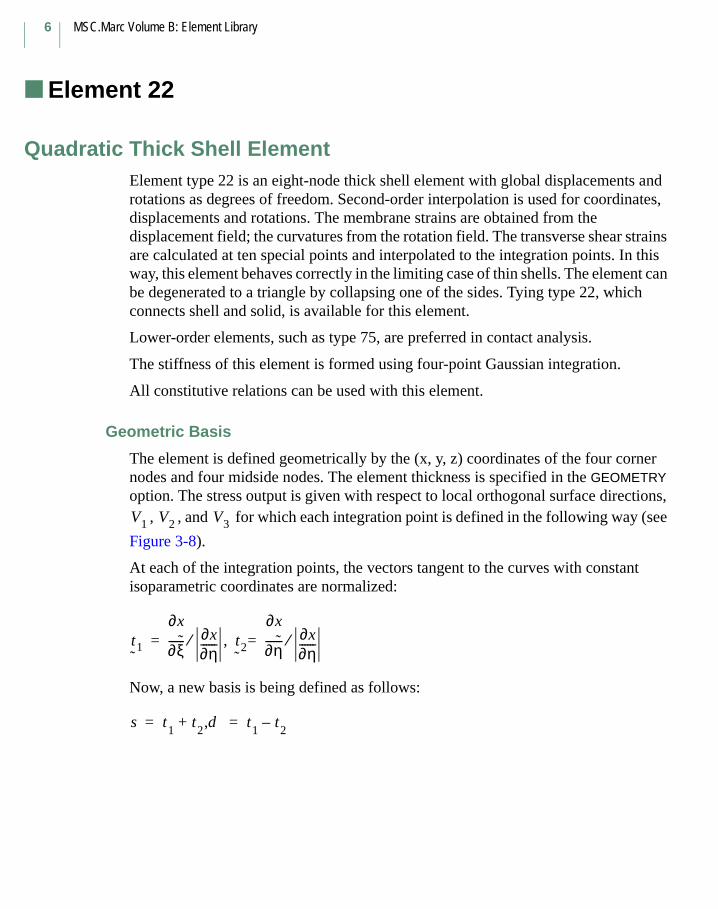
MSC.Marc Volume B: Element Library
6
Element 22
Quadratic Thick Shell ElementElement type 22 is an eight-node thick shell element with global displacements and rotations as degrees of freedom. Second-order interpolation is used for coordinates, displacements and rotations. The membrane strains are obtained from the displacement field; the curvatures from the rotation field. The transverse shear strains are calculated at ten special points and interpolated to the integration points. In this way, this element behaves correctly in the limiting case of thin shells. The element can be degenerated to a triangle by collapsing one of the sides. Tying type 22, which connects shell and solid, is available for this element.
Lower-order elements, such as type 75, are preferred in contact analysis.
The stiffness of this element is formed using four-point Gaussian integration.
All constitutive relations can be used with this element.
Geometric Basis
The element is defined geometrically by the (x, y, z) coordinates of the four corner nodes and four midside nodes. The element thickness is specified in the GEOMETRY option. The stress output is given with respect to local orthogonal surface directions,
, , and for which each integration point is defined in the following way (see
Figure 3-8).
At each of the integration points, the vectors tangent to the curves with constant isoparametric coordinates are normalized:
Now, a new basis is being defined as follows:
V1 V2 V3
t˜
1
∂x˜∂ξ
------ ∂x∂η------⁄ t
˜2,
∂x˜∂η
------ ∂x∂η------⁄= =
s t1
t2
d ,+ t1
t2
–= =
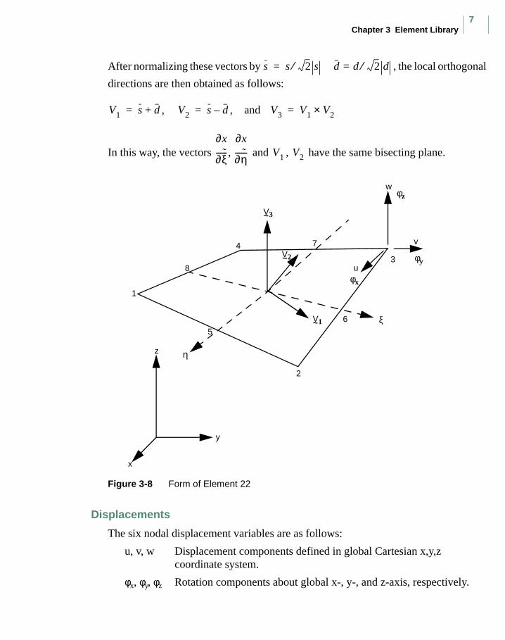
Chapter 3 Element Library7
After normalizing these vectors by , the local orthogonal
directions are then obtained as follows:
, , and
In this way, the vectors and , have the same bisecting plane.
Figure 3-8 Form of Element 22
Displacements
The six nodal displacement variables are as follows:
u, v, w Displacement components defined in global Cartesian x,y,z coordinate system.
φx, φy, φz Rotation components about global x-, y-, and z-axis, respectively.
s s 2 s d⁄ d 2 d⁄==
V1 s d+= V2 s d–= V3 V1 V2×=
∂x˜∂ξ
------,∂x
˜∂η------ V1 V2
1
2
3
4
η
ξ
z
y
x
V3~
V2~
V1~
8
5
7
6
v
uφx
φy
φzw

MSC.Marc Volume B: Element Library
8
Quick Reference
Type 22
Bilinear, eight-node shell element including transverse shear effects.
Connectivity
Eight nodes per element. The element can be collapsed to a triangle.
Geometry
Bilinear thickness variation is allowed in the plane of the element. Thicknesses at first, second, third, and fourth nodes of the element are stored for each element in the first (EGEOM1), second (EGEOM2), third (EGEOM3) and fourth (EGEOM4), geometry data fields, respectively. If EGEOM2 = EGEOM3 = EGEOM4 = 0, then a constant thickness (EGEOM1) is assumed for the element.
Note that the NODAL THICKNESS model definition option can also be used for the input of element thickness.
Coordinates
Three coordinates per node in the global x-, y-, and z-direction.
Degrees of Freedom
Six degrees of freedom per node:
1 = u = global (Cartesian) x-displacement2 = v = global (Cartesian) y-displacement3 = w = global (Cartesian) z-displacement4 = φx = rotation about global x-axis5 = φy = rotation about global y-axis6 = φz = rotation about global z-axis
Distributed Loads
Distributed load types follow below:
Load Type Description
1 Uniform gravity load per surface area in -z-direction.
2 Uniform pressure with positive magnitude in -V3-direction.
3 Nonuniform gravity load per surface area in -z-direction; magnitude given in the FORCEM user subroutine.
4 Nonuniform pressure with positive magnitude in -V3-direction; magnitude given in the FORCEM user subroutine.

Chapter 3 Element Library9
Point loads and moments can also be applied at the nodes.
5 Nonuniform load per surface area in arbitrary direction; magnitude given in the FORCEM user subroutine.
11 Uniform edge load in the plane of the surface on the 1-2 edge and perpendicular to this edge.
12 Nonuniform edge load; magnitude given in the FORCEM user subroutine in the plane of the surface on the 1-2 edge.
13 Nonuniform edge load; magnitude and direction given in the FORCEM user subroutine on 1-2 edge.
21 Uniform edge load in the plane of the surface on the 2-3 edge and perpendicular to this edge.
22 Nonuniform edge load; magnitude given in the FORCEM user subroutine in the plane of the surface on 2-3 edge.
23 Nonuniform edge load; magnitude and direction given in the FORCEM user subroutine on 2-3 edge.
31 Uniform edge load in the plane of the surface on the 3-4 edge and perpendicular to this edge.
32 Nonuniform edge load; magnitude given in the FORCEM user subroutine in the plane of the surface on 3-4 edge.
33 Nonuniform edge load; magnitude and direction given in the FORCEM user subroutine on 3-4 edge.
41 Uniform edge load in the plane of the surface on the 4-1 edge and perpendicular to this edge.
42 Nonuniform edge load; magnitude given in the FORCEM user subroutine in the plane of the surface on 4-1 edge.
43 Nonuniform edge load; magnitude and direction given in the FORCEM user subroutine on 4-1 edge.
100 Centrifugal load, magnitude represents square of angular velocity [rad/time]. Rotation axis specified in the ROTATION A option.
102 Gravity loading in global direction. Enter 3 magnitudes of gravity acceleration in respectively global x, y, z direction.
103 Coriolis and centrifugal load; magnitude represents square of angular velocity [rad/time]. Rotation axis is specified in the ROTATION A option.
Load Type Description
MSC.Marc Volume B: Element Library
10
Output of Strains
Generalized strain components are as follows:
Middle surface stretches:ε11 ε22 ε12
Middle surface curvatures:κ11 κ22 κ12
Transverse shear strains:γ23 γ31
in local ( , , ) system.
Output of Stresses
σ11, σ22, σ12, σ23, σ31 in local ( , , ) system given at equally spaced layers
though thickness. First layer is on positive V3 direction surface.
Transformation
Displacement and rotation at each node can be transformed to local direction.
Tying
Use the UFORMS user subroutine.
Updated Lagrange Procedure and Finite Strain Plasticity
Updated Lagrange capability is available. Note, however, that since the curvature calculation is linearized, you have to select your loadsteps such that the rotation remains small within a load step. Thickness is only updated if the FINITE parameter is specified.
Section Stress – Integration
Integration through the shell thickness is performed numerically using Simpson’s rule. Use the SHELL SECT parameter to specify the number of integration points. This number must be odd.
Coupled Analysis
In a coupled thermal-mechanical analysis, the associated heat transfer element is type 85. See Element 85 for a description of the conventions used for entering the flux and film data for this element. Volumetric flux due to dissipation of plastic work specified with type 101.
Design Variables
The thickness can be considered as a design variable.
V1 V2 V3
V1 V2 V3

Chapter 3 Element Library11
Element 23
Three-dimensional 20-node Rebar ElementThis element is an isoparametric, three-dimensional, 20-node empty brick in which you can place single strain members such as reinforcing rods or cords (i.e., rebars). The element is then used in conjunction with the 20-node brick continuum element (e.g., elements 21, 35, 57, or 61) to represent cord reinforced composite materials. This technique allows the rebar and the filler to be represented accurately with respect to their stress distribution, so that separate constitutive theories can be used in each (e.g., cracking concrete and yield rebar). The position, size, and orientation of the rebars are input either via the REBAR option or via the REBAR user subroutine.
Integration
It is assumed that several “layers” of rebars are presented. The number of such “layers” is input by you via the REBAR option or, if the REBAR user subroutine is used, in the second element geometry field. A maximum number of five layers can be used within a rebar element. Each layer is assumed to be similar to a pair of opposite element faces (although the rebar direction is arbitrary), so that the “thickness” direction is from one of the element faces to its opposite one. For instance (see Figure 3-29), if the layer is similar to the 1, 2, 3, 4 and 5, 6, 7, 8 faces of the element, the “thickness” direction is from the 1, 2, 3, 4 face to 5, 6, 7, 8 face of the element. The element is integrated using a numerical scheme based on Gauss quadrature. Each layer contains four integration points (see Figure 3-29). At each such integration point on each layer, you must input (via either the REBAR option or the REBAR user subroutine) the position, equivalent thickness (or, alternatively, spacing and area of cross section), and orientation of the rebars. See MSC.Marc Volume C: Program Input for REBAR option or MSC.Marc Volume D: User Subroutines and Special Routines for the REBAR user subroutine.
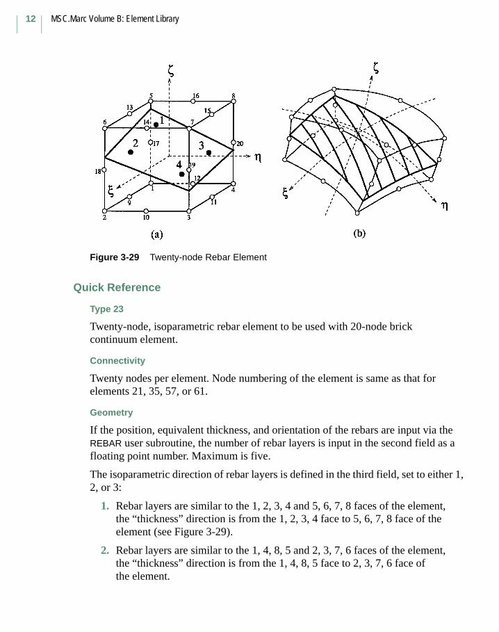
MSC.Marc Volume B: Element Library
12
Figure 3-29 Twenty-node Rebar Element
Quick Reference
Type 23
Twenty-node, isoparametric rebar element to be used with 20-node brick continuum element.
Connectivity
Twenty nodes per element. Node numbering of the element is same as that for elements 21, 35, 57, or 61.
Geometry
If the position, equivalent thickness, and orientation of the rebars are input via the REBAR user subroutine, the number of rebar layers is input in the second field as a floating point number. Maximum is five.
The isoparametric direction of rebar layers is defined in the third field, set to either 1, 2, or 3:
1. Rebar layers are similar to the 1, 2, 3, 4 and 5, 6, 7, 8 faces of the element, the “thickness” direction is from the 1, 2, 3, 4 face to 5, 6, 7, 8 face of the element (see Figure 3-29).
2. Rebar layers are similar to the 1, 4, 8, 5 and 2, 3, 7, 6 faces of the element, the “thickness” direction is from the 1, 4, 8, 5 face to 2, 3, 7, 6 face of the element.
Chapter 3 Element Library13
3. Rebar layers are similar to the 2, 1, 5, 6 and 3, 4, 8, 7 faces of the element, the “thickness” direction is from the 2, 1, 5, 6 face to 3, 4, 8, 7, face of the element.
The number of rebar layers and the isoparametric direction of the layers can also be defined using the REBAR model definition option.
Coordinates
Three global coordinates in the x-, y-, and z-directions.
Degrees of Freedom
Displacement output in global components is as follows:
1 – u2 – v3 – w
Tractions
Point loads can be applied at the nodes, but no distributed loads are available. Distributed loads are applied only to corresponding 20-node brick elements (e.g., element types 21, 35, 57, or 61).
Output of Strains and Stresses
One stress and one strain are output at each integration point – the axial rebar value. For the case of large deformations, the stress is the second Piola-Kirchhoff stress and the strain is the Green strain.
By using post code 471 and 481 (representing Second Piola Kirchhoff stress in undeformed configuration and Cauchy stress in deformed configuration, respectively), the rebar stress can be written into the post file in the form of a stress tensor defined in the global coordinate directions. Mentat can be used to plot the principal directions of the stress tensor to show the magnitude of rebar stress, rebar orientation, and their changes based on deformation.
Transformation
Any local set (u,v,w) can be used at any node.
Special Consideration
Either the REBAR option or the REBAR user subroutine is needed to input the position, size, and orientation of the rebars.
Updated Lagrange Procedure and Finite Strain Plasticity
Capability is not available.
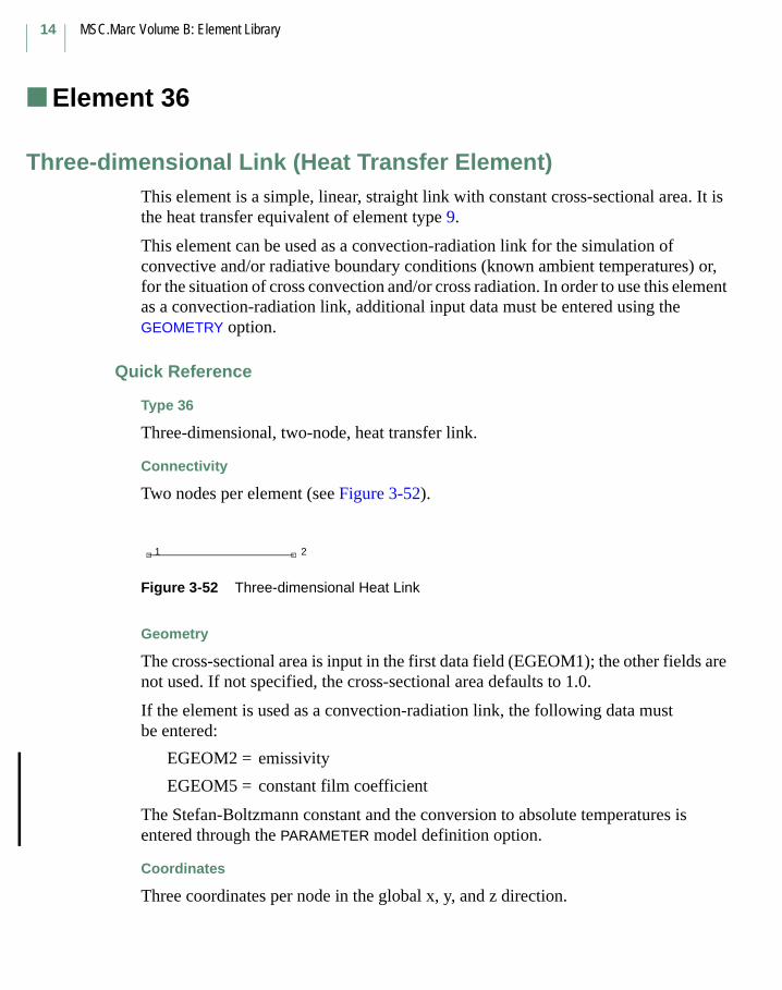
MSC.Marc Volume B: Element Library
14
Element 36
Three-dimensional Link (Heat Transfer Element)This element is a simple, linear, straight link with constant cross-sectional area. It is the heat transfer equivalent of element type 9.
This element can be used as a convection-radiation link for the simulation of convective and/or radiative boundary conditions (known ambient temperatures) or, for the situation of cross convection and/or cross radiation. In order to use this element as a convection-radiation link, additional input data must be entered using the GEOMETRY option.
Quick Reference
Type 36
Three-dimensional, two-node, heat transfer link.
Connectivity
Two nodes per element (see Figure 3-52).
Figure 3-52 Three-dimensional Heat Link
Geometry
The cross-sectional area is input in the first data field (EGEOM1); the other fields are not used. If not specified, the cross-sectional area defaults to 1.0.
If the element is used as a convection-radiation link, the following data must be entered:
EGEOM2 = emissivity
EGEOM5 = constant film coefficient
The Stefan-Boltzmann constant and the conversion to absolute temperatures is entered through the PARAMETER model definition option.
Coordinates
Three coordinates per node in the global x, y, and z direction.
21
Chapter 3 Element Library15
Degrees of Freedom
One degree of freedom per node:
1 = temperature
Fluxes
Distributed fluxes according to value of IBODY are as follows:
Films
Same specification as Fluxes.
Tying
Use the UFORMS user subroutine.
Joule Heating
Capability is available.
Current
Same specification as Fluxes.
Output Points
A single value at the centroid is given.
Flux Type Description
0 Uniform flux on first node (per cross-sectional area).
1 Volumetric flux on entire element (per volume).
2 Nonuniform flux given in the FLUX user subroutine on first node (per cross-sectional area).
3 Nonuniform volumetric flux given in the FLUX user subroutine on entire element (per volume).
MSC.Marc Volume B: Element Library
16
Element 46
Eight-node Plane Strain Rebar ElementThis element is isoparametric, plane strain, 8-node hollow quadrilateral in which you can place single strain members such as reinforcing rods or cords (that is, rebars). The element is then used in conjunction with the 8-node plane strain continuum element (for example, element 27 or 32) to represent cord reinforced composite materials. This technique allows the rebar and the filler to be represented accurately with respect to their stress distribution, so that separate constitutive theories can be used in each (e.g., cracking concrete and yield rebar). The position, size, and orientation of the rebars are input either via the REBAR option or via the REBAR user subroutine.
Integration
It is assumed that several “layers” of rebars are presented. The number of such “layers” is input by you via REBAR option or, if the REBAR user subroutine is used, in the second element geometry field. A maximum number of five layers can be used within a rebar element. Each layer is assumed to be similar to a pair of opposite element edges (although the rebar direction is arbitrary), so that the “thickness” direction is from one of the element edges to its opposite one. For instance (see Figure 3-64), if the layer is similar to the 1, 2 and 3, 4 edges of the element, the “thickness” direction is from the 1, 2 edge to 3, 4 edge of the element. The element is integrated using a numerical scheme based on Gauss quadrature. Each layer contains two integration points. At each such integration point on each layer, you must input, via either the REBAR option or the REBAR user subroutine, the position, equivalent thickness (or, alternatively, spacing and area of cross section), and orientation of the rebars. See MSC.Marc Volume C: Program Input for REBAR option or MSC.Marc Volume D: User Subroutines and Special Routines for the REBAR user subroutine.
Quick Reference
Type 46
Eight-node, isoparametric rebar element to be used with 8-node plane strain continuum element.
Connectivity
Eight nodes per element. Node numbering of the element is same as that for element 27 or 32.
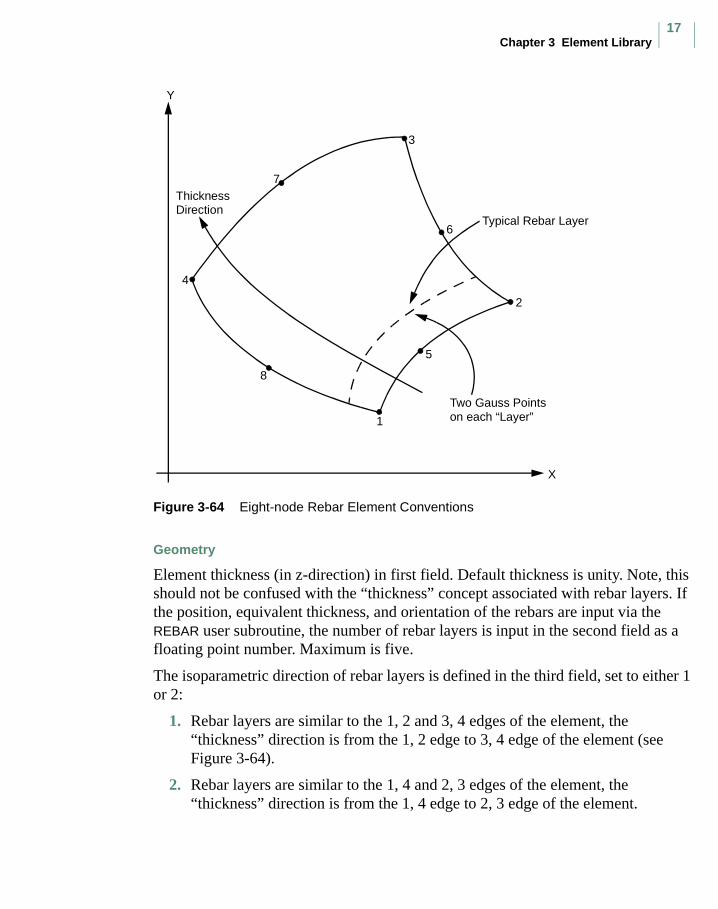
Chapter 3 Element Library17
Figure 3-64 Eight-node Rebar Element Conventions
Geometry
Element thickness (in z-direction) in first field. Default thickness is unity. Note, this should not be confused with the “thickness” concept associated with rebar layers. If the position, equivalent thickness, and orientation of the rebars are input via the REBAR user subroutine, the number of rebar layers is input in the second field as a floating point number. Maximum is five.
The isoparametric direction of rebar layers is defined in the third field, set to either 1 or 2:
1. Rebar layers are similar to the 1, 2 and 3, 4 edges of the element, the “thickness” direction is from the 1, 2 edge to 3, 4 edge of the element (see Figure 3-64).
2. Rebar layers are similar to the 1, 4 and 2, 3 edges of the element, the “thickness” direction is from the 1, 4 edge to 2, 3 edge of the element.
Typical Rebar Layer
Two Gauss Pointson each “Layer”1
2
3
4
5
6
7
8
ThicknessDirection
Y
X
MSC.Marc Volume B: Element Library
18
The number of rebar layers and the isoparametric direction of the layers can also be defined using the REBAR model definition option.
Coordinates
Two global coordinates x- and y-directions.
Degrees of Freedom
Displacement output in global components is as follows:
1 - u2 - v
Tractions
Point loads can be applied at the nodes, but no distributed loads are available. Distributed loads are applied only to corresponding 8-node plane strain elements (for example, element types 27 or 32).
Output of Stress and Strain
One stress and one strain are output at each integration point – the axial rebar value. For the case of large deformations, the stress is the second Piola-Kirchhoff stress and the strain is the Green strain.
By using post code 471 and 481 (representing Second Piola Kirchhoff stress in undeformed configuration and Cauchy stress in deformed configuration, respectively), the rebar stress can be written into the post file in the form of a stress tensor defined in the global coordinate directions. Mentat can be used to plot the principal directions of the stress tensor to show the magnitude of rebar stress, rebar orientation, and their changes based on deformation.
Transformation
Any local set (u,v) can be used at any node.
Special Consideration
Either REBAR option or the REBAR user subroutine is needed to input the position, size, and orientation of the rebars.
Updated Lagrange Procedure and Finite Strain Plasticity
Capability is not available.
Chapter 3 Element Library19
Element 86
Eight-node Curved Shell (Heat Transfer Element)This is a eight-node heat transfer shell element with temperatures as nodal degrees of freedom. Quadratic interpolation is used for the temperatures in the plane of the shell and either a linear or a quadratic temperature distribution is assumed in the shell thickness direction (see the HEAT parameter). A nine-point Gaussian integration is chosen for the element in the plane of the shell and Simpson’s rule is used in the thickness direction. This element can be used in conjunction with three-dimensional heat transfer brick elements through tying for heat transfer analysis. Note that only centroid or four Gaussian points are used for the output of element temperatures.
Geometric Basis
Similar to element type 22, the element is defined geometrically by the (x, y, z) coordinates of the four corner nodes and four midside nodes. The element thickness is specified in the GEOMETRY option. Local orthogonal surface directions (V1, V2, and V3) for each integration point are defined below (see Figure 3-65):
At each of the integration points, the vectors tangent to the curves with constant isoparametric coordinates are normalized.
Now a new basis is being defined as:
After normalizing these vectors by:
,
the local orthogonal directions are then obtained as:
, , and
In this way, the vectors , and V1, V2 have the same bisecting plane.
t1∂x∂ξ------ ∂x
∂ξ------⁄ , t2∂x∂η------ ∂x
∂η------⁄= =
s t1 t2, d+ t1 t2–= =
s s 2 s( )⁄= d d 2 d( )⁄=
V1 s d+= V2 s d–= V3 V1 V2×=
∂x∂ξ------
∂x∂η------
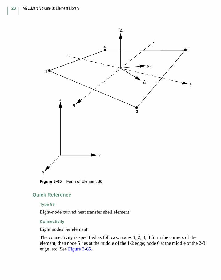
MSC.Marc Volume B: Element Library
20
Figure 3-65 Form of Element 86
Quick Reference
Type 86
Eight-node curved heat transfer shell element.
Connectivity
Eight nodes per element.
The connectivity is specified as follows: nodes 1, 2, 3, 4 form the corners of the element, then node 5 lies at the middle of the 1-2 edge; node 6 at the middle of the 2-3 edge, etc. See Figure 3-65.
1
2
34
η
ξ
z
y
x
V3~
V2~
V1~
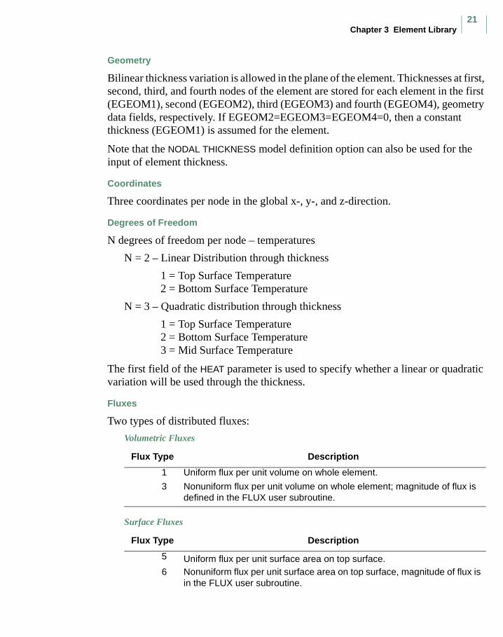
Chapter 3 Element Library21
Geometry
Bilinear thickness variation is allowed in the plane of the element. Thicknesses at first, second, third, and fourth nodes of the element are stored for each element in the first (EGEOM1), second (EGEOM2), third (EGEOM3) and fourth (EGEOM4), geometry data fields, respectively. If EGEOM2=EGEOM3=EGEOM4=0, then a constant thickness (EGEOM1) is assumed for the element.
Note that the NODAL THICKNESS model definition option can also be used for the input of element thickness.
Coordinates
Three coordinates per node in the global x-, y-, and z-direction.
Degrees of Freedom
N degrees of freedom per node – temperatures
N = 2 – Linear Distribution through thickness
1 = Top Surface Temperature2 = Bottom Surface Temperature
N = 3 – Quadratic distribution through thickness
1 = Top Surface Temperature2 = Bottom Surface Temperature3 = Mid Surface Temperature
The first field of the HEAT parameter is used to specify whether a linear or quadratic variation will be used through the thickness.
Fluxes
Two types of distributed fluxes:
Volumetric Fluxes
Surface Fluxes
Flux Type Description
1 Uniform flux per unit volume on whole element.
3 Nonuniform flux per unit volume on whole element; magnitude of flux is defined in the FLUX user subroutine.
Flux Type Description
5 Uniform flux per unit surface area on top surface.6 Nonuniform flux per unit surface area on top surface, magnitude of flux is
in the FLUX user subroutine.
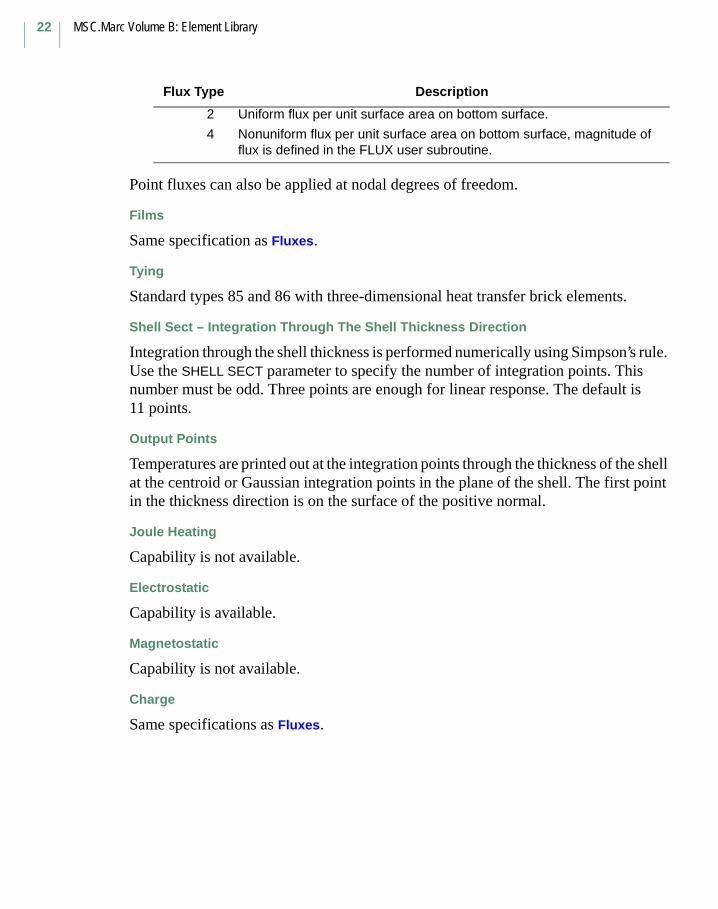
MSC.Marc Volume B: Element Library
22
Point fluxes can also be applied at nodal degrees of freedom.
Films
Same specification as Fluxes.
Tying
Standard types 85 and 86 with three-dimensional heat transfer brick elements.
Shell Sect – Integration Through The Shell Thickness Direction
Integration through the shell thickness is performed numerically using Simpson’s rule. Use the SHELL SECT parameter to specify the number of integration points. This number must be odd. Three points are enough for linear response. The default is 11 points.
Output Points
Temperatures are printed out at the integration points through the thickness of the shell at the centroid or Gaussian integration points in the plane of the shell. The first point in the thickness direction is on the surface of the positive normal.
Joule Heating
Capability is not available.
Electrostatic
Capability is available.
Magnetostatic
Capability is not available.
Charge
Same specifications as Fluxes.
2 Uniform flux per unit surface area on bottom surface.
4 Nonuniform flux per unit surface area on bottom surface, magnitude of flux is defined in the FLUX user subroutine.
Flux Type Description

Chapter 3 Element Library23
Element 109
Eight-node 3-D Magnetostatic ElementThis is an eight-node 3-D magnetostatic element with linear interpolation functions. It is similar to element type 43. The coefficient matrix is numerically integrated using eight (2 x 2 x 2) integration points.
Quick Reference
Type 109
Eight-node 3-D magnetostatic element.
Connectivity
Eight nodes per element.
See Figure 3-170 for numbering. Nodes 1-4 are the corners on one face, numbered in a counterclockwise direction when viewed from inside the element. Nodes 5-8 are the nodes on the other face, with node 5 opposite node 1, and so on.
Figure 3-170 Eight-node 3-D Magnetostatic Element
Coordinates
Three coordinates in the global x-, y-, and z-directions.
4
5
6
8
7
1
2
3
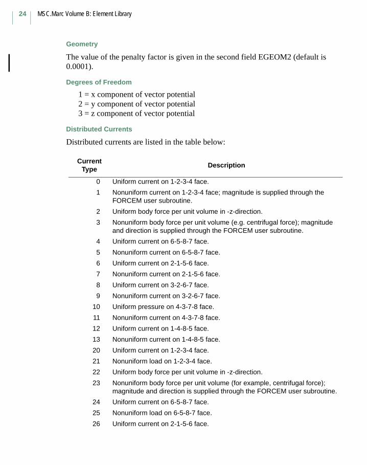
MSC.Marc Volume B: Element Library
24
Geometry
The value of the penalty factor is given in the second field EGEOM2 (default is 0.0001).
Degrees of Freedom
1 = x component of vector potential2 = y component of vector potential3 = z component of vector potential
Distributed Currents
Distributed currents are listed in the table below:
Current Type
Description
0 Uniform current on 1-2-3-4 face.
1 Nonuniform current on 1-2-3-4 face; magnitude is supplied through the FORCEM user subroutine.
2 Uniform body force per unit volume in -z-direction.
3 Nonuniform body force per unit volume (e.g. centrifugal force); magnitude and direction is supplied through the FORCEM user subroutine.
4 Uniform current on 6-5-8-7 face.
5 Nonuniform current on 6-5-8-7 face.
6 Uniform current on 2-1-5-6 face.
7 Nonuniform current on 2-1-5-6 face.
8 Uniform current on 3-2-6-7 face.
9 Nonuniform current on 3-2-6-7 face.
10 Uniform pressure on 4-3-7-8 face.
11 Nonuniform current on 4-3-7-8 face.
12 Uniform current on 1-4-8-5 face.
13 Nonuniform current on 1-4-8-5 face.
20 Uniform current on 1-2-3-4 face.
21 Nonuniform load on 1-2-3-4 face.
22 Uniform body force per unit volume in -z-direction.
23 Nonuniform body force per unit volume (for example, centrifugal force); magnitude and direction is supplied through the FORCEM user subroutine.
24 Uniform current on 6-5-8-7 face.
25 Nonuniform load on 6-5-8-7 face.
26 Uniform current on 2-1-5-6 face.
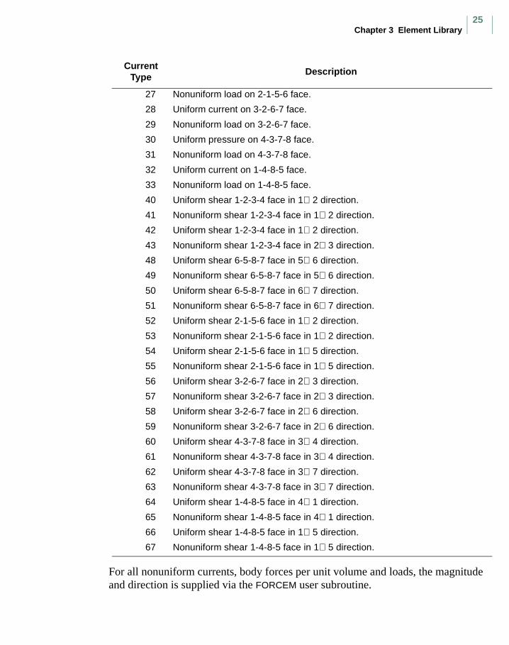
Chapter 3 Element Library25
For all nonuniform currents, body forces per unit volume and loads, the magnitude and direction is supplied via the FORCEM user subroutine.
27 Nonuniform load on 2-1-5-6 face.
28 Uniform current on 3-2-6-7 face.
29 Nonuniform load on 3-2-6-7 face.
30 Uniform pressure on 4-3-7-8 face.
31 Nonuniform load on 4-3-7-8 face.
32 Uniform current on 1-4-8-5 face.
33 Nonuniform load on 1-4-8-5 face.
40 Uniform shear 1-2-3-4 face in 1⇒ 2 direction.
41 Nonuniform shear 1-2-3-4 face in 1⇒ 2 direction.
42 Uniform shear 1-2-3-4 face in 1⇒ 2 direction.
43 Nonuniform shear 1-2-3-4 face in 2⇒ 3 direction.
48 Uniform shear 6-5-8-7 face in 5⇒ 6 direction.
49 Nonuniform shear 6-5-8-7 face in 5⇒ 6 direction.
50 Uniform shear 6-5-8-7 face in 6⇒ 7 direction.
51 Nonuniform shear 6-5-8-7 face in 6⇒ 7 direction.
52 Uniform shear 2-1-5-6 face in 1⇒ 2 direction.
53 Nonuniform shear 2-1-5-6 face in 1⇒ 2 direction.
54 Uniform shear 2-1-5-6 face in 1⇒ 5 direction.
55 Nonuniform shear 2-1-5-6 face in 1⇒ 5 direction.
56 Uniform shear 3-2-6-7 face in 2⇒ 3 direction.
57 Nonuniform shear 3-2-6-7 face in 2⇒ 3 direction.
58 Uniform shear 3-2-6-7 face in 2⇒ 6 direction.
59 Nonuniform shear 3-2-6-7 face in 2⇒ 6 direction.
60 Uniform shear 4-3-7-8 face in 3⇒ 4 direction.
61 Nonuniform shear 4-3-7-8 face in 3⇒ 4 direction.
62 Uniform shear 4-3-7-8 face in 3⇒ 7 direction.
63 Nonuniform shear 4-3-7-8 face in 3⇒ 7 direction.
64 Uniform shear 1-4-8-5 face in 4⇒ 1 direction.
65 Nonuniform shear 1-4-8-5 face in 4⇒ 1 direction.
66 Uniform shear 1-4-8-5 face in 1⇒ 5 direction.
67 Nonuniform shear 1-4-8-5 face in 1⇒ 5 direction.
Current Type
Description

MSC.Marc Volume B: Element Library
26
Currents are positive into element face.
Joule Heating
Capability is not available.
Electrostatic
Capability is not available.
Magnetostatic
Capability is available.
Output Points
Centroid or eight Gaussian integration points.
Tying
Use the UFORMS user subroutine.
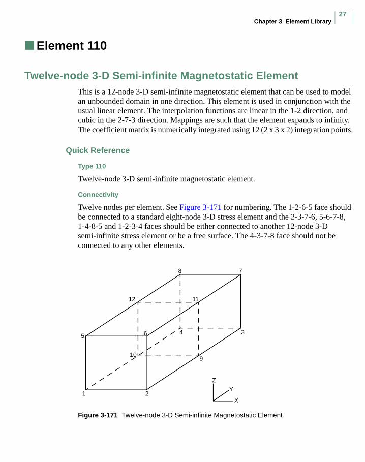
Chapter 3 Element Library27
Element 110
Twelve-node 3-D Semi-infinite Magnetostatic ElementThis is a 12-node 3-D semi-infinite magnetostatic element that can be used to model an unbounded domain in one direction. This element is used in conjunction with the usual linear element. The interpolation functions are linear in the 1-2 direction, and cubic in the 2-7-3 direction. Mappings are such that the element expands to infinity. The coefficient matrix is numerically integrated using 12 (2 x 3 x 2) integration points.
Quick Reference
Type 110
Twelve-node 3-D semi-infinite magnetostatic element.
Connectivity
Twelve nodes per element. See Figure 3-171 for numbering. The 1-2-6-5 face should be connected to a standard eight-node 3-D stress element and the 2-3-7-6, 5-6-7-8, 1-4-8-5 and 1-2-3-4 faces should be either connected to another 12-node 3-D semi-infinite stress element or be a free surface. The 4-3-7-8 face should not be connected to any other elements.
Figure 3-171 Twelve-node 3-D Semi-infinite Magnetostatic Element
1 2
345 6
78
910
1112
Z
Y
X
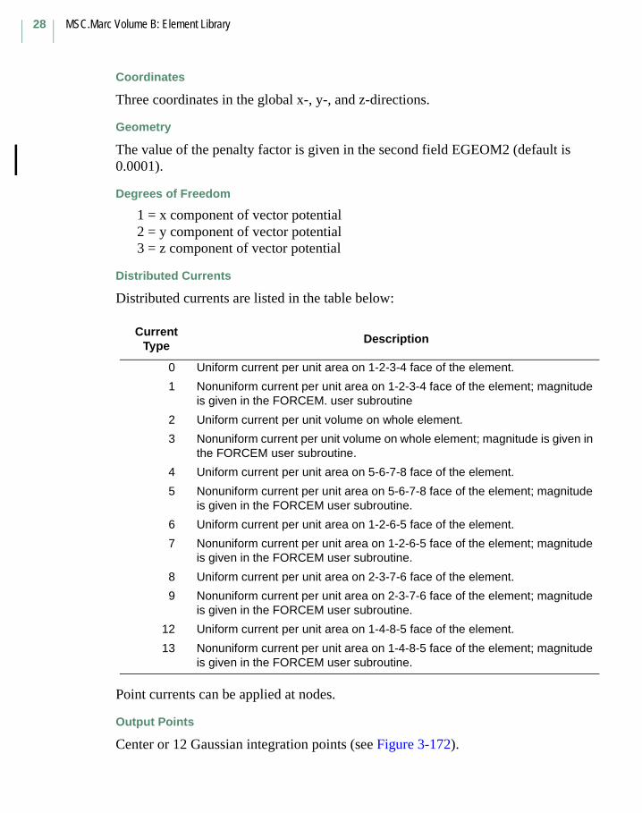
MSC.Marc Volume B: Element Library
28
Coordinates
Three coordinates in the global x-, y-, and z-directions.
Geometry
The value of the penalty factor is given in the second field EGEOM2 (default is 0.0001).
Degrees of Freedom
1 = x component of vector potential2 = y component of vector potential3 = z component of vector potential
Distributed Currents
Distributed currents are listed in the table below:
Point currents can be applied at nodes.
Output Points
Center or 12 Gaussian integration points (see Figure 3-172).
Current Type
Description
0 Uniform current per unit area on 1-2-3-4 face of the element.
1 Nonuniform current per unit area on 1-2-3-4 face of the element; magnitude is given in the FORCEM. user subroutine
2 Uniform current per unit volume on whole element.
3 Nonuniform current per unit volume on whole element; magnitude is given in the FORCEM user subroutine.
4 Uniform current per unit area on 5-6-7-8 face of the element.
5 Nonuniform current per unit area on 5-6-7-8 face of the element; magnitude is given in the FORCEM user subroutine.
6 Uniform current per unit area on 1-2-6-5 face of the element.
7 Nonuniform current per unit area on 1-2-6-5 face of the element; magnitude is given in the FORCEM user subroutine.
8 Uniform current per unit area on 2-3-7-6 face of the element.
9 Nonuniform current per unit area on 2-3-7-6 face of the element; magnitude is given in the FORCEM user subroutine.
12 Uniform current per unit area on 1-4-8-5 face of the element.
13 Nonuniform current per unit area on 1-4-8-5 face of the element; magnitude is given in the FORCEM user subroutine.
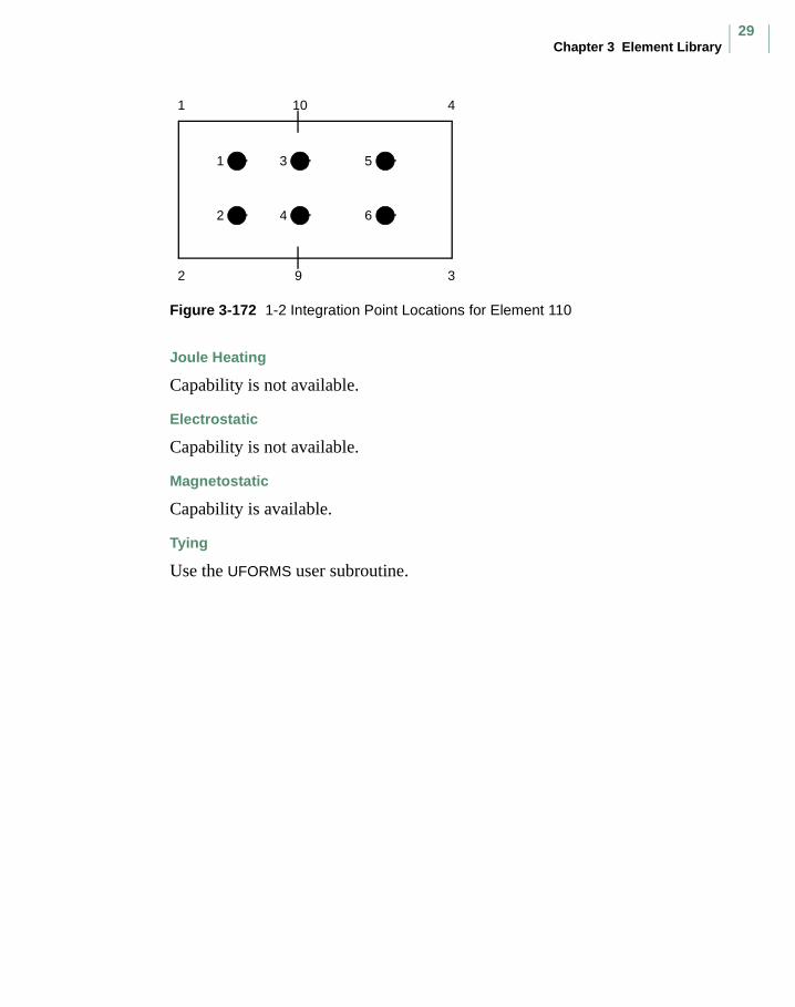
Chapter 3 Element Library29
Figure 3-172 1-2 Integration Point Locations for Element 110
Joule Heating
Capability is not available.
Electrostatic
Capability is not available.
Magnetostatic
Capability is available.
Tying
Use the UFORMS user subroutine.
1 3 5
2 4 6
1 10 4
2 9 3
MSC.Marc Volume B: Element Library
30
Element 142
Eight-node Axisymmetric Rebar Element with TwistThis element is similar to element 48, but is written for axisymmetric applications with torsional strains. It is a hollow, isoparametric 8-node quadrilateral in which you can place single strain members such as reinforcing rods or cords (i.e., rebars). The element is then used in conjunction with the 8-node axisymmetric continuum element with twist (for example, element 66 or 67) to represent cord reinforced composite materials. This technique allows the rebar and the filler to be represented accurately with respect to their stress distribution, so that separate constitutive theories can be used in each (for example, cracking concrete and yield rebar). The position, size, and orientation of the rebars are input either via the REBAR option or the REBAR user subroutine.
Integration
It is assumed that several “layers” of rebars are presented. The number of such “layers” is input by you via the REBAR option or, if the REBAR user subroutine is used, in the second element geometry field. A maximum number of five layers can be used within a rebar element. Each layer is assumed to be similar to a pair of opposite element edges (although the rebar direction is arbitrary), so that the “thickness” direction is from one of the element edges to its opposite one. For instance (see Figure 3-213), if the layer is similar to the 1, 2 and 3, 4 edges of the element, the “thickness” direction is from the 1, 2 edge to 3, 4 edge of the element. The element is integrated using a numerical scheme based on Gauss quadrature. Each layer contains two integration points.
At each such integration point on each layer, you must input (via either the REBAR option or the REBAR user subroutine) the position, equivalent thickness (or, alternatively, spacing and area of cross section), and orientation of the rebars. See MSC.Marc Volume C: Program Input for the REBAR option or MSC.Marc Volume D: User Subroutines and Special Routines for the REBAR user subroutine.
Quick Reference
Type 142
Eight-node, isoparametric rebar element with torsional strains.
Connectivity
Eight nodes per element. Node numbering of the element is same as that for element 66 or 67.
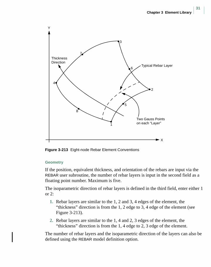
Chapter 3 Element Library31
Figure 3-213 Eight-node Rebar Element Conventions
Geometry
If the position, equivalent thickness, and orientation of the rebars are input via the REBAR user subroutine, the number of rebar layers is input in the second field as a floating point number. Maximum is five.
The isoparametric direction of rebar layers is defined in the third field, enter either 1 or 2:
1. Rebar layers are similar to the 1, 2 and 3, 4 edges of the element, the “thickness” direction is from the 1, 2 edge to 3, 4 edge of the element (see Figure 3-213).
2. Rebar layers are similar to the 1, 4 and 2, 3 edges of the element, the “thickness” direction is from the 1, 4 edge to 2, 3 edge of the element.
The number of rebar layers and the isoparametric direction of the layers can also be defined using the REBAR model definition option.
Typical Rebar Layer
Two Gauss Pointson each “Layer”1
2
3
4
5
6
7
8
ThicknessDirection
Y
X

MSC.Marc Volume B: Element Library
32
Coordinates
Two global coordinates in z- and r-directions.
Degrees of Freedom
Displacement output in global components is as follows:
1 - z2 - r3 - θ
Tractions
Point loads can be applied at the nodes but no distributed loads are available. Distributed loads are applied only to corresponding 8-node axisymmetric element with twist (for example, element types 66 or 67).
Output of Stress and Strain
One stress and one strain are output at each integration point – the axial rebar value. For the case of large deformations, the stress is the second Piola-Kirchhoff stress and the strain is the Green strain.
By using post code 471 and 481 (representing Second Piola Kirchhoff stress in undeformed configuration and Cauchy stress in deformed configuration, respectively), the rebar stress can be written into the post file in the form of a stress tensor defined in the global coordinate directions. Mentat can be used to plot the principal directions of the stress tensor to show the magnitude of rebar stress, rebar orientation, and their changes based on deformation.
Transformations
Any local set (u,v) can be used in the (z-r) plane at any node.
Special Considerations
Either the REBAR option or the REBAR user subroutine is needed to input the position, size, and orientation of the rebars.
Updated Lagrange Procedure and Finite Strain Plasticity
Capability is not available.
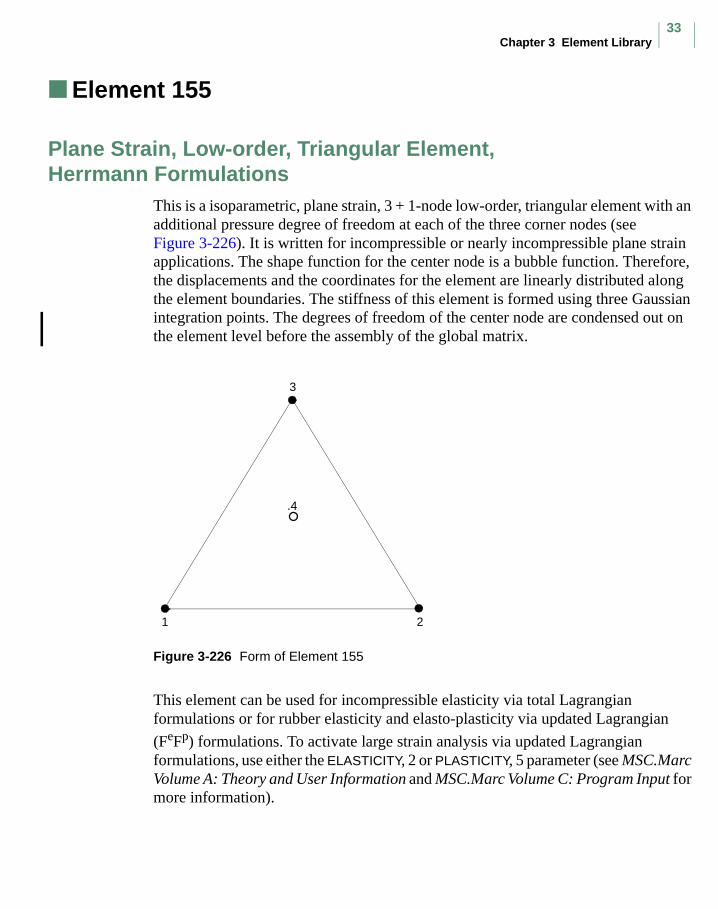
Chapter 3 Element Library33
Element 155
Plane Strain, Low-order, Triangular Element, Herrmann Formulations
This is a isoparametric, plane strain, 3 + 1-node low-order, triangular element with an additional pressure degree of freedom at each of the three corner nodes (see Figure 3-226). It is written for incompressible or nearly incompressible plane strain applications. The shape function for the center node is a bubble function. Therefore, the displacements and the coordinates for the element are linearly distributed along the element boundaries. The stiffness of this element is formed using three Gaussian integration points. The degrees of freedom of the center node are condensed out on the element level before the assembly of the global matrix.
Figure 3-226 Form of Element 155
This element can be used for incompressible elasticity via total Lagrangian formulations or for rubber elasticity and elasto-plasticity via updated Lagrangian
(FeFp) formulations. To activate large strain analysis via updated Lagrangian formulations, use either the ELASTICITY, 2 or PLASTICITY, 5 parameter (see MSC.Marc Volume A: Theory and User Information and MSC.Marc Volume C: Program Input for more information).
3
21
.4

MSC.Marc Volume B: Element Library
34
Integration
Three integration points are used to correctly interpolate the cubic shape function.
Quick Reference
Type 155
3 + 1-node, isoparametric, plane strain, triangular element using Herrmann formulation. Written for incompressible or nearly incompressible applications.
Connectivity
Four nodes per element (see Figure 3-226). Node numbering for the first three nodes is the same as for element type 6; that is, counterclockwise at three corners. The fourth node is located at the element center.
Geometry
Thickness of the element stored in the first data field (EGEOM1). Default thickness is unity. Other fields are not used.
Coordinates
Two global coordinates in the x- and y-directions. Marc automatically calculates the coordinates of the fourth (center) node of the element.
Degrees of Freedom
Displacement output in global components is:
1 - u2 - v
3 - p
Distributed Loads
Load types for distributed loads are as follows:
Load Type Description
0 Uniform pressure distributed on 1-2 face of the element.
1 Uniform body force per unit volume in first coordinate direction.
2 Uniform body force per unit volume in second coordinate direction.
3 Nonuniform pressure on 1-2 face of the element; magnitude supplied through the FORCEM user subroutine.
4 Nonuniform body force per unit volume in first coordinate direction; magnitude supplied through the FORCEM user subroutine.

Chapter 3 Element Library35
Output of Strain and Stresses
Stresses and Strains are output at each integration point. For the case of large deformations, the stresses are the second Piola-Kirchhoff stresses and the strains are the Green strains.
1 = global xx strain2 = global yy strain3 = global zz strain4 = global xy strain
If only element type 155, 156, or 157 is used in an analysis, the post file contains only one integration point for each element. The element stresses and strains in the point are the averaged results over three integration points of the element. This is to reduce the size of the post file.
Transformation
Any local set (u, v) can be used at any node.
Updated Lagrange Procedure and Finite Strain Plasticity
Capability is available with the ELASTICITY, 2 or PLASTICITY, 5 parameter.
5 Nonuniform body force per unit volume in second coordinate direction; magnitude supplied through the FORCEM user subroutine.
6 Uniform pressure on 2-3 face of the element.
7 Nonuniform pressure on 2-3 face of the element; magnitude supplied through the FORCEM user subroutine.
8 Uniform pressure on 3-1 face of the element.
9 Nonuniform pressure on 3-1 face of the element; magnitude supplied through the FORCEM user subroutine.
100 Centrifugal load; magnitude represents square angular velocity [rad/time]. Rotation axis is specified in the ROTATION A option.
102 Gravity loading in global direction. Enter three magnitudes of gravity acceleration in the x-, y-, and z-direction.
103 Coriolis and centrifugal load; magnitude represents square of angular velocity [rad/time]. Rotation axis is specified in the ROTATION A option.
Load Type Description
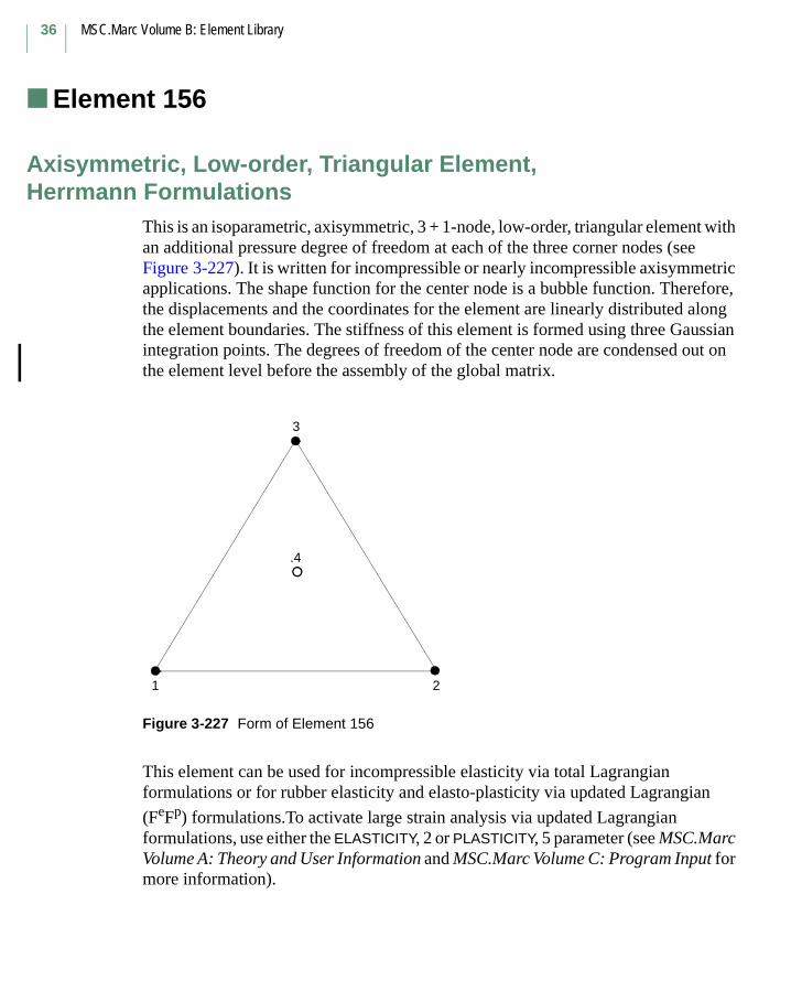
MSC.Marc Volume B: Element Library
36
Element 156
Axisymmetric, Low-order, Triangular Element, Herrmann Formulations
This is an isoparametric, axisymmetric, 3 + 1-node, low-order, triangular element with an additional pressure degree of freedom at each of the three corner nodes (see Figure 3-227). It is written for incompressible or nearly incompressible axisymmetric applications. The shape function for the center node is a bubble function. Therefore, the displacements and the coordinates for the element are linearly distributed along the element boundaries. The stiffness of this element is formed using three Gaussian integration points. The degrees of freedom of the center node are condensed out on the element level before the assembly of the global matrix.
Figure 3-227 Form of Element 156
This element can be used for incompressible elasticity via total Lagrangian formulations or for rubber elasticity and elasto-plasticity via updated Lagrangian
(FeFp) formulations.To activate large strain analysis via updated Lagrangian formulations, use either the ELASTICITY, 2 or PLASTICITY, 5 parameter (see MSC.Marc Volume A: Theory and User Information and MSC.Marc Volume C: Program Input for more information).
3
21
.4
Chapter 3 Element Library37
Integration
Three integration points are used to correctly interpolate the cubic shape function.
Quick Reference
Type 156
3 + 1-node, isoparametric, axisymmetric, triangular element using Herrmann formulation. Written for incompressible or nearly incompressible applications.
Connectivity
Four nodes per element (see Figure 3-227). Node numbering for the first three nodes is the same as for element type 2; that is, counterclockwise at three corners. The fourth node is located at the element center.
Coordinates
Two global coordinates in the z- and r-directions. Marc automatically calculates the coordinates of the fourth (center) node of the element.
Degrees of Freedom
1 - u2 - v3 - p
Distributed Loads
Load types for distributed loads are as follows:
Load Type Description
0 Uniform pressure distributed on 1-2 face of the element.
1 Uniform body force per unit volume in first coordinate direction.
2 Uniform body force per unit volume in second coordinate direction.
3 Nonuniform pressure on 1-2 face of the element; magnitude supplied through the FORCEM user subroutine.
4 Nonuniform body force per unit volume in first coordinate direction; magnitude supplied through the FORCEM user subroutine.
5 Nonuniform body force per unit volume in second coordinate direction; magnitude supplied through the FORCEM user subroutine.
6 Uniform pressure on 2-3 face of the element.
7 Nonuniform pressure on 2-3 face of the element; magnitude supplied through the FORCEM user subroutine.

MSC.Marc Volume B: Element Library
38
All pressures are positive when directed into the element. In addition, point loads can be applied at the nodes.
Concentrated loads applied at the nodes must be the value of the load integrated around the circumference.
Output of Strain and Stresses
Stresses and Strains are output at each integration point. For the case of large deformations, the stresses are the second Piola-Kirchhoff stresses and the strains are the Green strains.
1 = global zz strain2 = global rr strain3 = global θθ strain4 = global zr strain
If only element type 155, 156, or 157 is used in an analysis, the post file contains only one integration point for each element. The element stresses and strains in the point are the averaged results over three integration points of the element. This is to reduce the size of the post file.
Updated Lagrange Procedure and Finite Strain Plasticity
Capability is available with the ELASTICITY, 2 or PLASITICITY, 5 parameter.
8 Uniform pressure on 3-1 face of the element.
9 Nonuniform pressure on 3-1 face of the element; magnitude supplied through the FORCEM user subroutine.
100 Centrifugal load; magnitude represents square angular velocity [rad/time]. Rotation axis is specified in the ROTATION A option.
102 Gravity loading in global direction. Enter three magnitudes of gravity acceleration in the x-, y-, and z-direction.
103 Coriolis and centrifugal load; magnitude represents square of angular velocity [rad/time]. Rotation axis is specified in the ROTATION A option.
Load Type Description
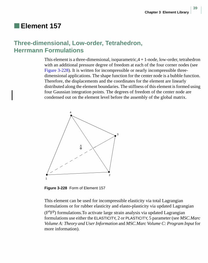
Chapter 3 Element Library39
Element 157
Three-dimensional, Low-order, Tetrahedron, Herrmann Formulations
This element is a three-dimensional, isoparametric,4 + 1-node, low-order, tetrahedron with an additional pressure degree of freedom at each of the four corner nodes (see Figure 3-228). It is written for incompressible or nearly incompressible three-dimensional applications. The shape function for the center node is a bubble function. Therefore, the displacements and the coordinates for the element are linearly distributed along the element boundaries. The stiffness of this element is formed using four Gaussian integration points. The degrees of freedom of the center node are condensed out on the element level before the assembly of the global matrix.
Figure 3-228 Form of Element 157
This element can be used for incompressible elasticity via total Lagrangian formulations or for rubber elasticity and elasto-plasticity via updated Lagrangian
(FeFp) formulations.To activate large strain analysis via updated Lagrangian formulations use either the ELASTICITY, 2 or PLASTICITY, 5 parameter (see MSC.Marc Volume A: Theory and User Information and MSC.Marc Volume C: Program Input for more information).
2
3
4
1
.5
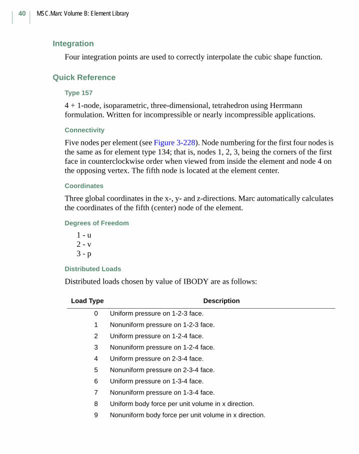
MSC.Marc Volume B: Element Library
40
Integration
Four integration points are used to correctly interpolate the cubic shape function.
Quick Reference
Type 157
4 + 1-node, isoparametric, three-dimensional, tetrahedron using Herrmann formulation. Written for incompressible or nearly incompressible applications.
Connectivity
Five nodes per element (see Figure 3-228). Node numbering for the first four nodes is the same as for element type 134; that is, nodes 1, 2, 3, being the corners of the first face in counterclockwise order when viewed from inside the element and node 4 on the opposing vertex. The fifth node is located at the element center.
Coordinates
Three global coordinates in the x-, y- and z-directions. Marc automatically calculates the coordinates of the fifth (center) node of the element.
Degrees of Freedom
1 - u2 - v3 - p
Distributed Loads
Distributed loads chosen by value of IBODY are as follows:
Load Type Description
0 Uniform pressure on 1-2-3 face.
1 Nonuniform pressure on 1-2-3 face.
2 Uniform pressure on 1-2-4 face.
3 Nonuniform pressure on 1-2-4 face.
4 Uniform pressure on 2-3-4 face.
5 Nonuniform pressure on 2-3-4 face.
6 Uniform pressure on 1-3-4 face.
7 Nonuniform pressure on 1-3-4 face.
8 Uniform body force per unit volume in x direction.
9 Nonuniform body force per unit volume in x direction.
Chapter 3 Element Library41
Output of Strain and Stresses
Stresses and Strains are output at each integration point. For the case of large deformations, the stresses are the second Piola-Kirchhoff stresses and the strains are the Green strains.
1 = global xx strain2 = global yy strain3 = global zz strain4 = global xy strain5 = global yz strain6 = global zx strain
If only element type 155, 156, or 157 is used in an analysis, the post file contains only one integration point for each element. The element stresses and strains in the point are the averaged results over three integration points of the element. This is to reduce the size of the post file.
Transformation
Any local set (u, v, w) can be used at any node.
Updated Lagrange Procedure and Finite Strain Plasticity
Capability is available with parameter ELASTICITY, 2 or parameter PLASTICITY, 5.
10 Uniform body force per unit volume in y direction.
11 Nonuniform body force per unit volume in y direction.
12 Uniform body force per unit volume in z direction.
13 Nonuniform body force per unit volume in z direction.
100 Centrifugal load, magnitude represents square of angular velocity [rad/time]. Rotation axis is specified in the ROTATION A option.
102 Gravity loading in global direction. Enter three magnitudes of gravity acceleration in respectively global x, y, z direction.
103 Coriolis and centrifugal load; magnitude represents square of angular velocity [rad/time]. Rotation axis is specified in the ROTATION A option.
Load Type Description

MSC.Marc Volume B: Element Library
42

Volume C: Program Input1
Volume C: Program Input

MSC.Marc Volume C: Program Input
2

Chapter 2 Parameters3
Chapter 2 Parameters
MSC.Marc Volume C: Program Input
4
SUPER
Super Element Input
Description
This parameter allows for the input of stiffness and load terms generated by the SUBSTRUCTURE commands in a previous analysis. It can be used in a multilevel substructure definition in combination with the SUBSTRUC parameter or on the main level of a substructure analysis. If this parameter is used, no other elements are necessary; in which case, the ELEMENTS parameter is not used.
FormatFree Entry
DataTypeFixed
Format
1-5 1st A Enter the word SUPER.
11-15 2nd I Enter Fortran unit number for the data base containing the super element information.
16-20 3rd I Enter the maximum number of nodes in any super element.
21-25 4th I Enter the maximum number of degrees of freedom per node number in any super element.
26-30 5th I Enter the number of super elements in this analysis.
31-35 6th I = 0 Marc superelement created using SUBSTRUCTURE in previous Marc job.
= 1 Super element comes from an external program and all relevant data, except the connectivity specified in SUPERINPUT model definition data is created using the USSUBS user subroutine. In this case, the second entry should be left blank.

Chapter 2 Parameters5
NEW
Use New Format
Description
This parameter allows the input of data in the new Version K style format. Input is interpreted to be in this format until an OLD parameter is encountered. This parameter must not appear embedded inside a model definition or history definition option.
FormatFree Entry
DataTypeFixed
Format
1-10 1st A Enter the word NEW.
11-15 2nd I Enter 1 if the default width of the data fields is used for input. This will override the EXTENDED parameter.
Enter 2 if the double width of the data fields is used for input.

MSC.Marc Volume C: Program Input
6
OLD
Use Old Format
Description
This parameter allows the input of data in the old (Rev. G, H, J) style format. Input is interpreted to be in this format until a NEW parameter is encountered. This parameter must not appear embedded inside a model definition or history definition option.
FormatFree Entry
DataTypeFixed
Format
1-10 1st A Enter the word OLD.
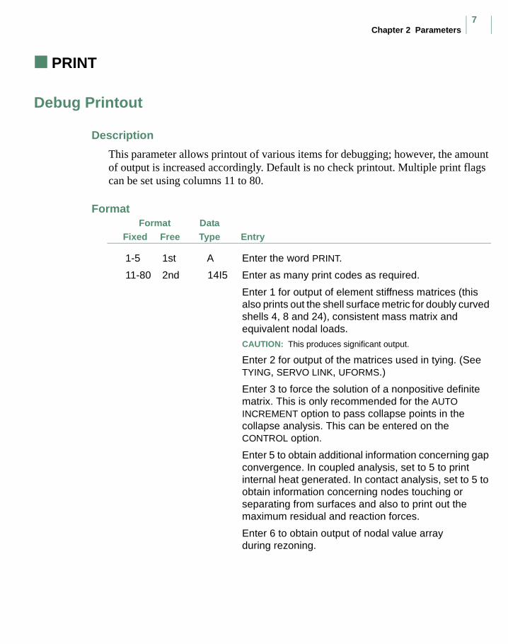
Chapter 2 Parameters7
Debug Printout
Description
This parameter allows printout of various items for debugging; however, the amount of output is increased accordingly. Default is no check printout. Multiple print flags can be set using columns 11 to 80.
FormatFree Entry
DataTypeFixed
Format
1-5 1st A Enter the word PRINT.
11-80 2nd 14I5 Enter as many print codes as required.
Enter 1 for output of element stiffness matrices (this also prints out the shell surface metric for doubly curved shells 4, 8 and 24), consistent mass matrix and equivalent nodal loads. CAUTION: This produces significant output.
Enter 2 for output of the matrices used in tying. (See TYING, SERVO LINK, UFORMS.)
Enter 3 to force the solution of a nonpositive definite matrix. This is only recommended for the AUTO INCREMENT option to pass collapse points in the collapse analysis. This can be entered on the CONTROL option.
Enter 5 to obtain additional information concerning gap convergence. In coupled analysis, set to 5 to print internal heat generated. In contact analysis, set to 5 to obtain information concerning nodes touching or separating from surfaces and also to print out the maximum residual and reaction forces.
Enter 6 to obtain output of nodal value array during rezoning.

MSC.Marc Volume C: Program Input
8
FormatFree Entry
DataTypeFixed
Enter 7 to obtain tying information in CONRAD GAP option and fluid element numbers in CHANNEL option which is used to define fluid channel input data in heat transfer analysis.
Enter 8 to obtain incremental displacements in local system in contact problems.
Enter 9 to obtain latent heat output.
Enter 10 to obtain the stress-strain relation in the local coordinate system.
Enter 11 to obtain additional information on the interlaminar stress calculation.
Enter 12 to output the right hand side and solution vector.CAUTION: This produces significant output.
Enter 14 to obtain information regarding the mesh adapting process.

Chapter 2 Parameters9
FILMS
Film Coefficients and Sink Temperatures
Description
This parameter allows for the input of the maximum number of elements that have films. This parameter is not needed if the number of elements with films is not increased in the history definition section.
FormatFree Entry
DataTypeFixed
Format
1-10 1st A Enter the FILMS.
11-15 2nd I Maximum number of elements that have films.

MSC.Marc Volume C: Program Input
10
Chapter 3 Model Definition
Options

Chapter 3 Model Definition Options11
NEW (Model Definition)
Use New Format
Description
This option allows the input of data in the K style format. Input is interpreted to be in this format until an OLD option is encountered. This option must not appear embedded inside a model definition or history definition option.
FormatFree Entry
DataTypeFixed
Format
1-10 1st A Enter the word NEW.
11-15 2nd I Enter 1 if the default width of the data fields is used for input. This will override the EXTENDED parameter.
Enter 2 if the double width of the data fields is used for input.
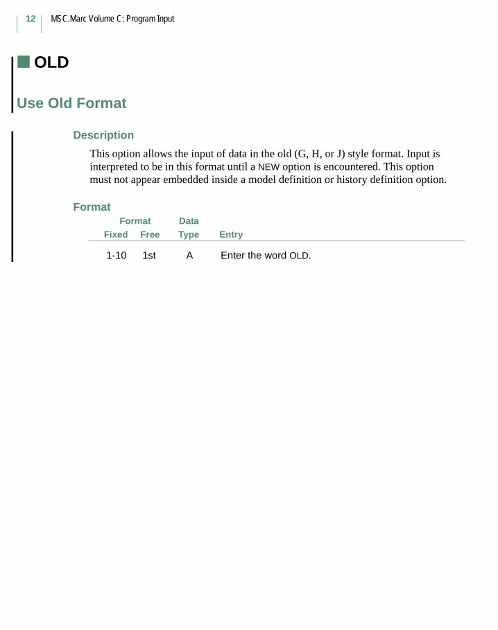
MSC.Marc Volume C: Program Input
12
OLD (Model Definition)
Use Old Format
Description
This option allows the input of data in the old (G, H, or J) style format. Input is interpreted to be in this format until a NEW option is encountered. This option must not appear embedded inside a model definition or history definition option.
FormatFree Entry
DataTypeFixed
Format
1-10 1st A Enter the word OLD.

Chapter 3 Model Definition Options13
WRITE
Write Connectivity and Coordinates
Description
This option allows you to write the final connectivity and coordinates to an auxiliary file. The values written are those after all internal mesh generations (MESH2D, FXORD or incremental generators) and all external (UFXORD, UFCONN) transformations have been performed. All node numbers are in the user system; that is, nonoptimized.
Note: The connectivity and coordinates data are written to the auxiliary file in the format (default or extended) based on the last related valid option (see the EXTENDED parameter as well as the NEW (model definition and history definition option) and OLD (model definition and history definition option) before the END OPTION line.
FormatFree Entry
DataTypeFixed
Format
1st data block
1-10 1st A Enter the word WRITE.
11-15 2nd I Enter the unit number to write to. Default is unit 1.
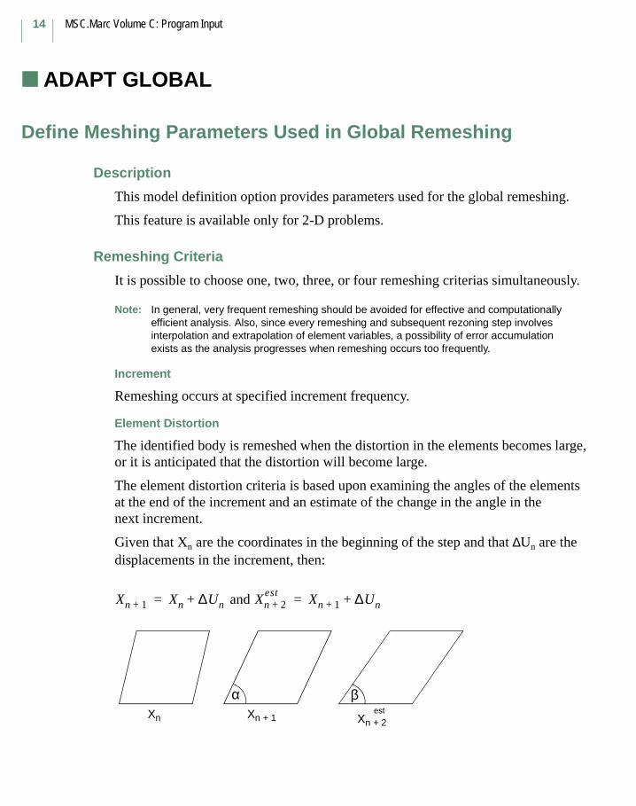
MSC.Marc Volume C: Program Input
14
ADAPT GLOBAL (Model Definition)
Define Meshing Parameters Used in Global Remeshing
Description
This model definition option provides parameters used for the global remeshing.
This feature is available only for 2-D problems.
Remeshing Criteria
It is possible to choose one, two, three, or four remeshing criterias simultaneously.
Note: In general, very frequent remeshing should be avoided for effective and computationally efficient analysis. Also, since every remeshing and subsequent rezoning step involves interpolation and extrapolation of element variables, a possibility of error accumulation exists as the analysis progresses when remeshing occurs too frequently.
Increment
Remeshing occurs at specified increment frequency.
Element Distortion
The identified body is remeshed when the distortion in the elements becomes large, or it is anticipated that the distortion will become large.
The element distortion criteria is based upon examining the angles of the elements at the end of the increment and an estimate of the change in the angle in the next increment.
Given that Xn are the coordinates in the beginning of the step and that ∆Un are the displacements in the increment, then:
and Xn 1+ Xn ∆Un+= Xn 2+est Xn 1+ ∆Un+=
Xn Xn + 1 Xn + 2est
α β

Chapter 3 Model Definition Options15
If cos α > 0.8 and cos β > 0.9, remesh, or if cos α > 0.9 and cos β > cos α, remesh
which is equivalent to
0 <α < 36° and 0<β<25° remesh or144°<α<180° and 155°<β<180° remesh or0<α<25° and β<α or155°<α<180° and β>α
Contact Penetration
The identified body is remeshed when the curvature of the contact body is such that the current mesh cannot accurately detect penetration.
The penetration remeshing criteria is based upon examining the distance between the edge of the element and the representation of the other contact surface.
If b> penetration limit, remeshing is required. By default, penetration is 2 * (contact tolerance). The contact tolerance can be input by you or computed internally by the program.
Please note that this check does not apply to the self-contact situation.
Angle Deviation
The identified body remeshes when the angles in the element have a deviation from the ideal angle greater than a specified amount. The ideal angle for quadrilaterals or hexahedrals is 90°. The ideal angle for triangles and tetrahedrals is 60°. The default of 40° indicates that any angle in the range 50< α < 130 is acceptable for quadrilaterals.
Immediate
The identified body is remeshed before performing any analysis.
b

MSC.Marc Volume C: Program Input
16
FormatFree Entry
DataTypeFixed
Format
1st data block
1-8 1st A Enter the words ADAPT GLOBAL.
2nd data block
1-5 1st I Enter the number of bodies to be remeshed.
6-10 2nd I Enter 0 for default.Enter the unit number to read data; defaults to input.
11-15 3rd I Not used; enter 0.
The third, fourth, and fifth data blocks are repeated based on the number of remeshing bodies selected in the 2nd data block.
3rd data block
1-5 1st I Enter 2 for Advancing Front 2-D quadrilateral or triangular mesher.
Enter 3 for Delaunay 2-D triangular mesher
Enter 4 for 2-D Overlay quadrilateral mesher.
A valid mesher type (2-4) must be used.
6-10 2nd I Not used; enter 0.
11-15 3rd I Enter the contact body to be remeshed (default = 1) where the contact body number is defined under the CONTACT option.
4th data block
1-5 1st I Enter 1 if increment frequency used as remesh criterion.
6-10 2nd I Enter 1 if element distortion used as remesh criterion.
11-15 3rd I Enter 1 if penetration is used as remesh criterion.
16-20 4th I If the first field is 1, enter the frequency in increments.
21-30 5th E Not used.
31-35 6th I Enter 1 if angle criterion is used.
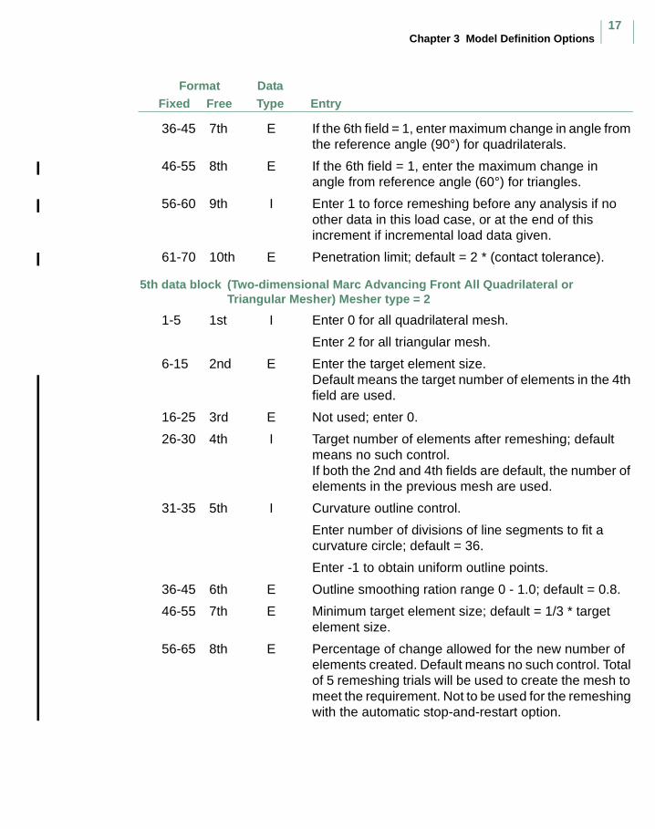
Chapter 3 Model Definition Options17
FormatFree Entry
DataTypeFixed
36-45 7th E If the 6th field = 1, enter maximum change in angle from the reference angle (90°) for quadrilaterals.
46-55 8th E If the 6th field = 1, enter the maximum change in angle from reference angle (60°) for triangles.
56-60 9th I Enter 1 to force remeshing before any analysis if no other data in this load case, or at the end of this increment if incremental load data given.
61-70 10th E Penetration limit; default = 2 * (contact tolerance).
5th data block (Two-dimensional Marc Advancing Front All Quadrilateral or Triangular Mesher) Mesher type = 2
1-5 1st I Enter 0 for all quadrilateral mesh.
Enter 2 for all triangular mesh.
6-15 2nd E Enter the target element size.Default means the target number of elements in the 4th field are used.
16-25 3rd E Not used; enter 0.
26-30 4th I Target number of elements after remeshing; default means no such control.If both the 2nd and 4th fields are default, the number of elements in the previous mesh are used.
31-35 5th I Curvature outline control.
Enter number of divisions of line segments to fit a curvature circle; default = 36.
Enter -1 to obtain uniform outline points.
36-45 6th E Outline smoothing ration range 0 - 1.0; default = 0.8.
46-55 7th E Minimum target element size; default = 1/3 * target element size.
56-65 8th E Percentage of change allowed for the new number of elements created. Default means no such control. Total of 5 remeshing trials will be used to create the mesh to meet the requirement. Not to be used for the remeshing with the automatic stop-and-restart option.

MSC.Marc Volume C: Program Input
18
FormatFree Entry
DataTypeFixed
5th data block (Two-dimensional Delaunay Triangular Mesher)Mesher type = 3
1-5 1st I Not used; enter 0.
6-15 2nd E Enter the target element size.
16-25 3rd E Not used; enter 0.
26-30 4th I Target number of elements after remeshing; default means no such control.
31-35 5th I Curvature outline control. Enter number of divisions of line segments to fit a curvature circle. Default = 36.
Enter -1 to obtain uniform outline points.
36-45 6th E Outline smoothing ratio (range 0-1.0); default = 0.8.
46-55 7th E Minimum target element size; default = 1/3 * target element size.
56-65 8th E Percentage of change allowed for the new number of elements created. Default means no such control. Totally 5 remeshing trials will be used to create the mesh to meet the requirement. Not to be used for the remeshing with the automatic stop-and-restart option.
5th data block (Two-dimensional Overlay Quadrilateral Mesher)Mesher type = 4
1-10 1st E Enter the element target length.
11-15 2nd I Enter 1 if elements on the boundary in contact are to be refined one level if necessary.
Enter 2 if elements on the boundary in contact are to be refined two levels if necessary.
16-20 3rd I Enter 1 if elements in the interior can be merged together. Four elements at a time will be merged.
21-25 4th I Target number of elements after remeshing; default means no such control.
26-30 5th I Not used; enter 0.
31-40 6th E Not used; enter 0.
41-50 7th E Not used, enter 0.
51-60 8th E Percentage of change allowed for the new number of elements created. Default means no such control. Totally 5 remeshing trials will be used to create the mesh to meet the requirement. Not to be used for the remeshing with the automatic stop-and-restart option.
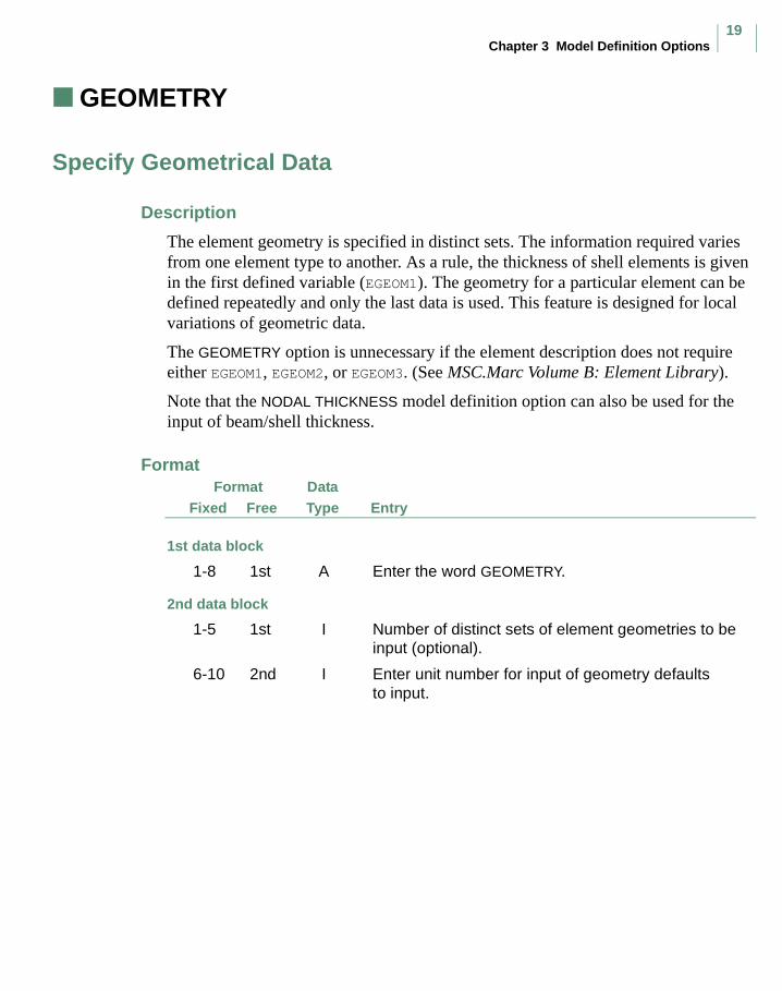
Chapter 3 Model Definition Options19
GEOMETRY
Specify Geometrical Data
Description
The element geometry is specified in distinct sets. The information required varies from one element type to another. As a rule, the thickness of shell elements is given in the first defined variable (EGEOM1). The geometry for a particular element can be defined repeatedly and only the last data is used. This feature is designed for local variations of geometric data.
The GEOMETRY option is unnecessary if the element description does not require either EGEOM1, EGEOM2, or EGEOM3. (See MSC.Marc Volume B: Element Library).
Note that the NODAL THICKNESS model definition option can also be used for the input of beam/shell thickness.
FormatFree Entry
DataTypeFixed
Format
1st data block
1-8 1st A Enter the word GEOMETRY.
2nd data block
1-5 1st I Number of distinct sets of element geometries to be input (optional).
6-10 2nd I Enter unit number for input of geometry defaults to input.
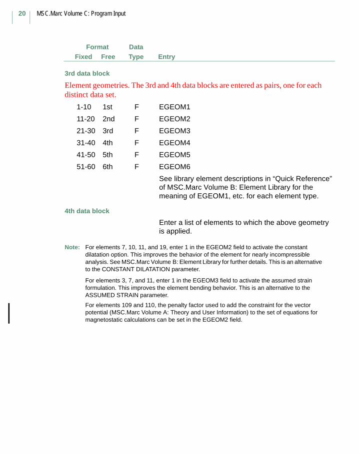
MSC.Marc Volume C: Program Input
20
FormatFree Entry
DataTypeFixed
3rd data block
Element geometries. The 3rd and 4th data blocks are entered as pairs, one for each distinct data set.
1-10 1st F EGEOM1
11-20 2nd F EGEOM2
21-30 3rd F EGEOM3
31-40 4th F EGEOM4
41-50 5th F EGEOM5
51-60 6th F EGEOM6
See library element descriptions in “Quick Reference” of MSC.Marc Volume B: Element Library for the meaning of EGEOM1, etc. for each element type.
4th data block
Enter a list of elements to which the above geometry is applied.
Note: For elements 7, 10, 11, and 19, enter 1 in the EGEOM2 field to activate the constant dilatation option. This improves the behavior of the element for nearly incompressible analysis. See MSC.Marc Volume B: Element Library for further details. This is an alternative to the CONSTANT DILATATION parameter.
For elements 3, 7, and 11, enter 1 in the EGEOM3 field to activate the assumed strain formulation. This improves the element bending behavior. This is an alternative to the ASSUMED STRAIN parameter.
For elements 109 and 110, the penalty factor used to add the constraint for the vector potential (MSC.Marc Volume A: Theory and User Information) to the set of equations for magnetostatic calculations can be set in the EGEOM2 field.
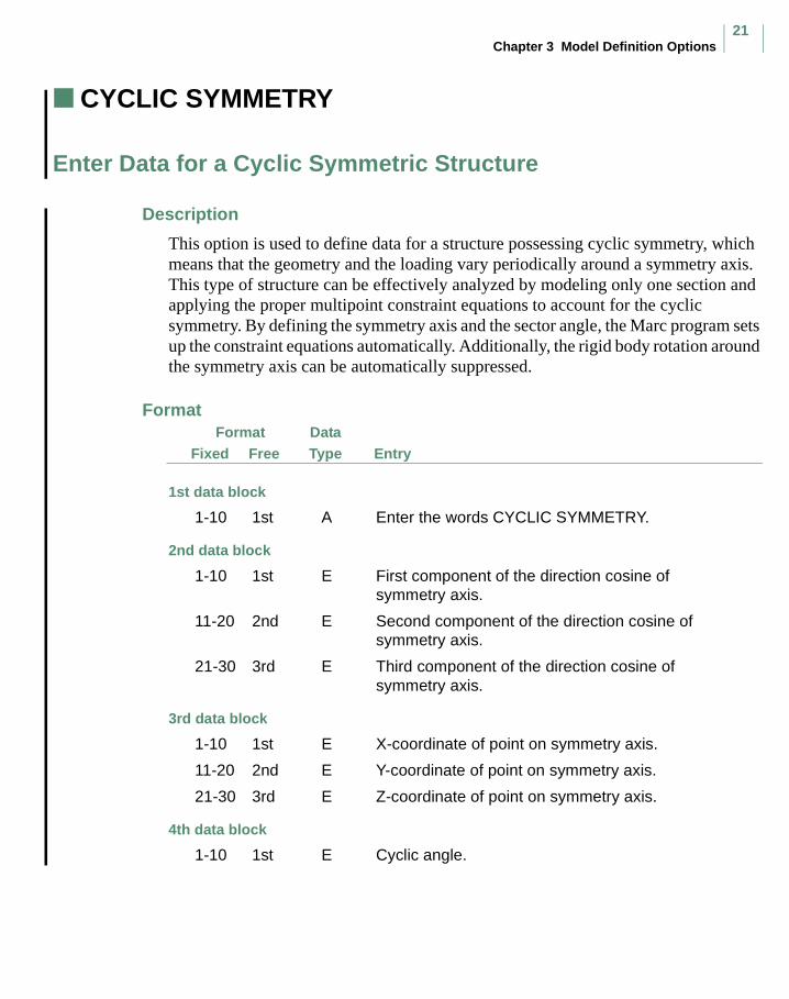
Chapter 3 Model Definition Options21
CYCLIC SYMMETRY
Enter Data for a Cyclic Symmetric Structure
Description
This option is used to define data for a structure possessing cyclic symmetry, which means that the geometry and the loading vary periodically around a symmetry axis. This type of structure can be effectively analyzed by modeling only one section and applying the proper multipoint constraint equations to account for the cyclic symmetry. By defining the symmetry axis and the sector angle, the Marc program sets up the constraint equations automatically. Additionally, the rigid body rotation around the symmetry axis can be automatically suppressed.
FormatFree Entry
DataTypeFixed
Format
1st data block
1-10 1st A Enter the words CYCLIC SYMMETRY.
2nd data block
1-10 1st E First component of the direction cosine of symmetry axis.
11-20 2nd E Second component of the direction cosine of symmetry axis.
21-30 3rd E Third component of the direction cosine of symmetry axis.
3rd data block
1-10 1st E X-coordinate of point on symmetry axis.
11-20 2nd E Y-coordinate of point on symmetry axis.
21-30 3rd E Z-coordinate of point on symmetry axis.
4th data block
1-10 1st E Cyclic angle.

MSC.Marc Volume C: Program Input
22
FormatFree Entry
DataTypeFixed
5th data block
1-5 1st I Enter:
-1 To automatically suppress rigid body mode.
0 To have no suppression.
>0 To supress at node number given.

Chapter 3 Model Definition Options23
CROSS-SECTION
Enter Data to Define Cross Sections
Description
This is option allows the definition of cross sections which can be used to simulate pre-stressed bolts or rivets. For each cross section, the option requires:
a. a special node associated with the cross section,
b. the normal to the cross section,
c. the nodes lying on the cross section and the elements connected to these nodes and lying on the side of the cross section corresponding to the negative normal direction.
FormatFree Entry
DataTypeFixed
Format
1st data block
1-10 1st A Enter the word CROSS-SECTION.
2nd data block
1-5 1st I Number of cross sections to be defined (optional).
6-10 2nd I Unit number for input of cross sections. Defaults to input.
3rd data block
1-5 1st I Cross section number.
5-10 2nd I Additional cross section node.
11-15 3rd I Enter a 2 to enter the list of nodes and elements given below.
4th data block
No data required.

MSC.Marc Volume C: Program Input
24
FormatFree Entry
DataTypeFixed
5th data block
1-10 1st F First component of normal to cross section.
11-20 2nd F Second component of normal to cross section.
21-30 3rd F Third component of normal to cross section.
6th data block
Enter the list of nodes in the cross section.
7th data block
Enter the list of elements.
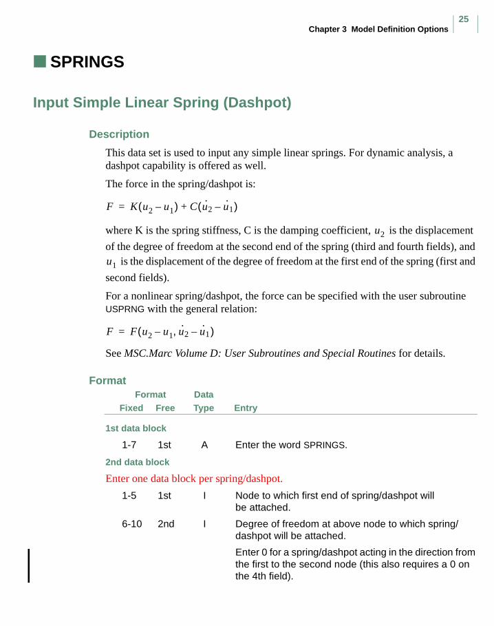
Chapter 3 Model Definition Options25
SPRINGS
Input Simple Linear Spring (Dashpot)
Description
This data set is used to input any simple linear springs. For dynamic analysis, a dashpot capability is offered as well.
The force in the spring/dashpot is:
where K is the spring stiffness, C is the damping coefficient, is the displacement
of the degree of freedom at the second end of the spring (third and fourth fields), and is the displacement of the degree of freedom at the first end of the spring (first and
second fields).
For a nonlinear spring/dashpot, the force can be specified with the user subroutine USPRNG with the general relation:
See MSC.Marc Volume D: User Subroutines and Special Routines for details.
FormatFree Entry
DataTypeFixed
Format
1st data block
1-7 1st A Enter the word SPRINGS.
2nd data block
Enter one data block per spring/dashpot.
1-5 1st I Node to which first end of spring/dashpot will be attached.
6-10 2nd I Degree of freedom at above node to which spring/dashpot will be attached.
Enter 0 for a spring/dashpot acting in the direction from the first to the second node (this also requires a 0 on the 4th field).
F K u2 u1–( ) C u·2 u·1–( )+=
u2
u1
F F u2 u1 u·2 u·1–,–( )=
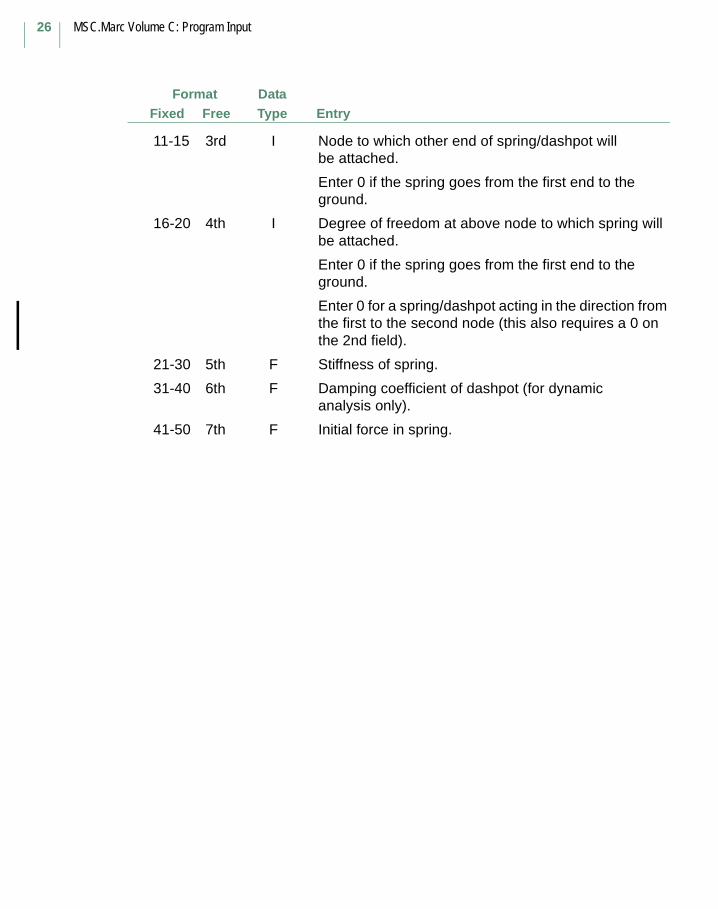
MSC.Marc Volume C: Program Input
26
FormatFree Entry
DataTypeFixed
11-15 3rd I Node to which other end of spring/dashpot will be attached.
Enter 0 if the spring goes from the first end to the ground.
16-20 4th I Degree of freedom at above node to which spring will be attached.
Enter 0 if the spring goes from the first end to the ground.
Enter 0 for a spring/dashpot acting in the direction from the first to the second node (this also requires a 0 on the 2nd field).
21-30 5th F Stiffness of spring.
31-40 6th F Damping coefficient of dashpot (for dynamic analysis only).
41-50 7th F Initial force in spring.
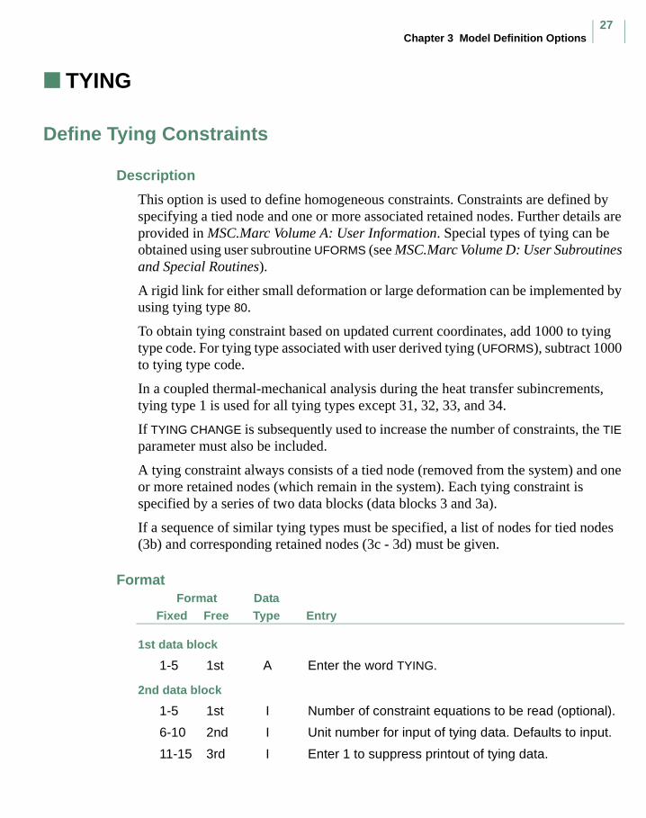
Chapter 3 Model Definition Options27
TYING
Define Tying Constraints
Description
This option is used to define homogeneous constraints. Constraints are defined by specifying a tied node and one or more associated retained nodes. Further details are provided in MSC.Marc Volume A: User Information. Special types of tying can be obtained using user subroutine UFORMS (see MSC.Marc Volume D: User Subroutines and Special Routines).
A rigid link for either small deformation or large deformation can be implemented by using tying type 80.
To obtain tying constraint based on updated current coordinates, add 1000 to tying type code. For tying type associated with user derived tying (UFORMS), subtract 1000 to tying type code.
In a coupled thermal-mechanical analysis during the heat transfer subincrements, tying type 1 is used for all tying types except 31, 32, 33, and 34.
If TYING CHANGE is subsequently used to increase the number of constraints, the TIE parameter must also be included.
A tying constraint always consists of a tied node (removed from the system) and one or more retained nodes (which remain in the system). Each tying constraint is specified by a series of two data blocks (data blocks 3 and 3a).
If a sequence of similar tying types must be specified, a list of nodes for tied nodes (3b) and corresponding retained nodes (3c - 3d) must be given.
FormatFree Entry
DataTypeFixed
Format
1st data block
1-5 1st A Enter the word TYING.
2nd data block
1-5 1st I Number of constraint equations to be read (optional).
6-10 2nd I Unit number for input of tying data. Defaults to input.
11-15 3rd I Enter 1 to suppress printout of tying data.
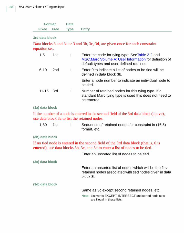
MSC.Marc Volume C: Program Input
28
FormatFree Entry
DataTypeFixed
3rd data block
Data blocks 3 and 3a or 3 and 3b, 3c, 3d, are given once for each constraint equation set.
1-5 1st I Enter the code for tying type. SeeTable 3-2 and MSC.Marc Volume A: User Information for definition of default types and user-defined routines.
6-10 2nd I Enter 0 to indicate a list of nodes to be tied will be defined in data block 3b.
Enter a node number to indicate an individual node to be tied.
11-15 3rd I Number of retained nodes for this tying type. If a standard Marc tying type is used this does not need to be entered.
(3a) data block
If the number of a node is entered in the second field of the 3rd data block (above), use data block 3a to list the retained nodes.
1-80 1st I Sequence of retained nodes for constraint in (16I5) format, etc.
(3b) data block
If no tied node is entered in the second field of the 3rd data block (that is, 0 is entered), use data blocks 3b, 3c, and 3d to enter a list of nodes to be tied.
Enter an unsorted list of nodes to be tied.
(3c) data block
Enter an unsorted list of nodes which will be the first retained nodes associated with tied nodes given in data block 3b.
(3d) data block
Same as 3c except second retained nodes, etc.Note: List verbs EXCEPT, INTERSECT and sorted node sets
are illegal in these lists.

Chapter 3 Model Definition Options29
Table 3-2 Summary of Standard Tying Types
Tying Code
Number of Retained
NodesPurpose Remarks
I<NDEG 1 Tie the Ith degree of freedom at the tied node to the Ith degree of freedom at the retained node
100 1 Tie all degrees of freedom at the tied node to the corresponding degrees of freedom at the retained node
23 1 Tie axisymmetric solid node to axisymmetric-shell (element type 1) node
Both tied and retained nodes must be transformed to local system. TRANSFORMATION option must be invoked. (See MSC.Marc Volume A: User Information, Table 9-17)
15 Number of retained nodes is 1 less than the number of shell nodes in the z-r plane of the section
Special tying types for pipe bend element 17 to remove rigid body modes (see Volume B: Element Library)
16 Number of shell nodes in the z-r plane of the section
Special tying types for pipe bend element 17 to remove rigid body modes (see Volume B: Element Library)
17 2 Special tying types for pipe bend element 17 to couple bend section into pipe line (see Volume B: Element Library)
18 2 Joining together the boundaries of intersecting shell, element type 4, 8 or 24. Fully moment carrying joint.
Tied node is also second retained node. Neither node can be transformed (see MSC.Marc Volume A: User Information, Table 9-15)
28 2 Joining intersecting shells, element type 4, 8, or 24. Pinned joint.
Tied node is also second retained node (see MSC.Marc Volume A: User Information, Table 9-15)
19 2 Use beam element 13 as a stiffener on shell elements 4 or 8. Tied node is beam node: First retained node is shell node, second is beam node again. Beam node should be on, or close to, the normal to the shell at the shell node.

MSC.Marc Volume C: Program Input
30
20 3 Create an extra node in a shell type 8 element tied to the interpolation function of the shell. Use in conjunction with tying type 21 to tie a beam element 13 or a stiffener across a shell element.
Always use after tying type 21.
21 2 Same as type 19, but tying beam to an interpolated shell node not as a vertex of an element – element type 8 only. Must be followed by type 20 to tie the interpolated shell node into the shell mesh.
Must be followed by a tying type 20.
24 2 Join intersecting shells or beams, element type 15-17.
Tied node is also second retained node. Neither node can be transformed. Tying is necessary only when there is a large angle between the two plates.
25 2 Join solid mesh to shell or beam (type 15 or 16).
Similar to 23, but no transformation needed. Tied node is also second retained node.
26 2 Join solid mesh to axisymmetric shell (type 1 or 89).
Similar to 5. Tied node is also second to retained node.
27 2 Join Fourier solid to Fourier shell (type 90). Tied node is also second retained node.
31 2 Refine mesh of first order (linear displacement) elements in 2-D.
Tie interior nodes on refined side to corner nodes on coarse side.
32 2 Refine mesh of second order (quadratic displacement) elements in 2-D.
Tie interior nodes on refined side to the edge of an element on the coarse side.
33 4 Refine mesh of 8-node bricks Tie interior node on the refined side to the 4 corner nodes of an element face on the coarse side.
34 8 Refine mesh of 20-node bricks Tie interior nodes on refined side to the 8 (4 corner, 4 midside) nodes of an element on the coarse side.
52 1 Pin joint for beam types 14, 25, or 52.
53 1 Fully moment carrying joint for beam types 14, 25, or 52.
13 2 Joining two elements type 13 under an arbitrary angle. Fully moment carrying joint.
Tied node is also the second retained node.
Table 3-2 Summary of Standard Tying Types (Continued)
Tying Code
Number of Retained
NodesPurpose Remarks
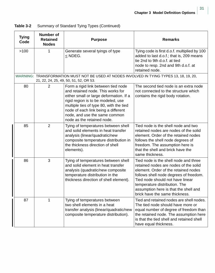
Chapter 3 Model Definition Options31
>100 1 Generate several tyings of type< NDEG.
Tying code is first d.o.f. multiplied by 100 added to last d.o.f.; that is, 209 means tie 2nd to 9th d.o.f. at tied node to resp. 2nd and 9th d.o.f. at retained node.
WARNING: TRANSFORMATION MUST NOT BE USED AT NODES INVOLVED IN TYING TYPES 13, 18, 19, 20, 21, 22, 24, 25, 49, 50, 51, 52, OR 53.
80 2 Form a rigid link between tied node and retained node. This works for either small or large deformation. If a rigid region is to be modeled, use multiple ties of type 80, with the tied node of each link being a different node, and use the same common node as the retained node.
The second tied node is an extra node not connected to the structure which contains the rigid body rotation.
85 2 Tying of temperatures between shell and solid elements in heat transfer analysis (linear/quadratic/new composite temperature distribution in the thickness direction of shell elements).
Tied node is the shell node and two retained nodes are nodes of the solid element. Order of the retained nodes follows the shell node degrees of freedom. The assumption here is that the shell and brick have the same thickness.
86 3 Tying of temperatures between shell and solid element in heat transfer analysis (quadratic/new composite temperature distribution in the thickness direction of shell element).
Tied node is the shell node and three retained nodes are nodes of the solid element. Order of the retained nodes follows shell node degrees of freedom. Tied node should not have linear temperature distribution. The assumption here is that the shell and brick have the same thickness.
87 1 Tying of temperatures between two shell elements in a heat transfer analysis (linear/quadratic/new composite temperature distribution).
Tied and retained nodes are shell nodes. The tied node should have more or equal number of degree of freedom than the retained node. The assumption here is that the tied shell and retained shell have equal thickness.
Table 3-2 Summary of Standard Tying Types (Continued)
Tying Code
Number of Retained
NodesPurpose Remarks
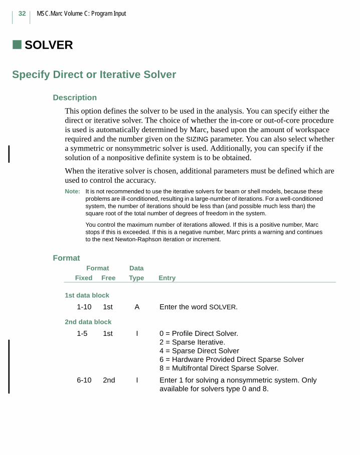
MSC.Marc Volume C: Program Input
32
SOLVER (Model Definition)
Specify Direct or Iterative Solver
Description
This option defines the solver to be used in the analysis. You can specify either the direct or iterative solver. The choice of whether the in-core or out-of-core procedure is used is automatically determined by Marc, based upon the amount of workspace required and the number given on the SIZING parameter. You can also select whether a symmetric or nonsymmetric solver is used. Additionally, you can specify if the solution of a nonpositive definite system is to be obtained.
When the iterative solver is chosen, additional parameters must be defined which are used to control the accuracy. Note: It is not recommended to use the iterative solvers for beam or shell models, because these
problems are ill-conditioned, resulting in a large-number of iterations. For a well-conditioned system, the number of iterations should be less than (and possible much less than) the square root of the total number of degrees of freedom in the system.
You control the maximum number of iterations allowed. If this is a positive number, Marc stops if this is exceeded. If this is a negative number, Marc prints a warning and continues to the next Newton-Raphson iteration or increment.
FormatFree Entry
DataTypeFixed
Format
1st data block
1-10 1st A Enter the word SOLVER.
2nd data block
1-5 1st I 0 = Profile Direct Solver.2 = Sparse Iterative.4 = Sparse Direct Solver6 = Hardware Provided Direct Sparse Solver8 = Multifrontal Direct Sparse Solver.
6-10 2nd I Enter 1 for solving a nonsymmetric system. Only available for solvers type 0 and 8.
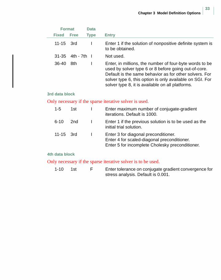
Chapter 3 Model Definition Options33
FormatFree Entry
DataTypeFixed
11-15 3rd I Enter 1 if the solution of nonpositive definite system is to be obtained.
31-35 4th - 7th I Not used.
36-40 8th I Enter, in millions, the number of four-byte words to be used by solver type 6 or 8 before going out-of-core. Default is the same behavior as for other solvers. For solver type 6, this option is only available on SGI. For solver type 8, it is available on all platforms.
3rd data block
Only necessary if the sparse iterative solver is used.
1-5 1st I Enter maximum number of conjugate-gradient iterations. Default is 1000.
6-10 2nd I Enter 1 if the previous solution is to be used as the initial trial solution.
11-15 3rd I Enter 3 for diagonal preconditioner.Enter 4 for scaled-diagonal preconditioner.Enter 5 for incomplete Cholesky preconditioner.
4th data block
Only necessary if the sparse iterative solver is to be used.
1-10 1st F Enter tolerance on conjugate gradient convergence for stress analysis. Default is 0.001.
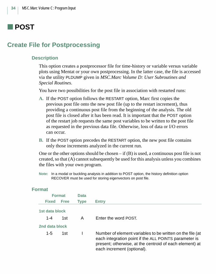
MSC.Marc Volume C: Program Input
34
POST
Create File for Postprocessing
Description
This option creates a postprocessor file for time-history or variable versus variable plots using Mentat or your own postprocessing. In the latter case, the file is accessed via the utility PLDUMP given in MSC.Marc Volume D: User Subroutines and Special Routines.
You have two possibilities for the post file in association with restarted runs:
A. If the POST option follows the RESTART option, Marc first copies the previous post file onto the new post file (up to the restart increment), thus providing a continuous post file from the beginning of the analysis. The old post file is closed after it has been read. It is important that the POST option of the restart job requests the same post variables to be written to the post file as requested in the previous data file. Otherwise, loss of data or I/O errors can occur.
B. If the POST option precedes the RESTART option, the new post file contains only those increments analyzed in the current run.
One or the other options should be chosen – if (B) is used, a continuous post file is not created, so that (A) cannot subsequently be used for this analysis unless you combines the files with your own program.
Note: In a modal or buckling analysis in addition to POST option, the history definition option RECOVER must be used for storing eigenvectors on post file.
FormatFree Entry
DataTypeFixed
Format
1st data block
1-4 1st A Enter the word POST.
2nd data block
1-5 1st I Number of element variables to be written on the file (at each integration point if the ALL POINTS parameter is present; otherwise, at the centroid of each element) at each increment (optional).
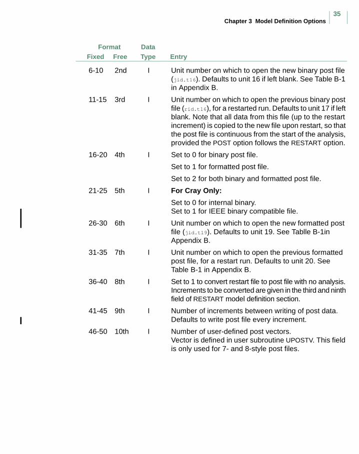
Chapter 3 Model Definition Options35
FormatFree Entry
DataTypeFixed
6-10 2nd I Unit number on which to open the new binary post file (jid.t16). Defaults to unit 16 if left blank. See Table B-1 in Appendix B.
11-15 3rd I Unit number on which to open the previous binary post file (rid.t16), for a restarted run. Defaults to unit 17 if left blank. Note that all data from this file (up to the restart increment) is copied to the new file upon restart, so that the post file is continuous from the start of the analysis, provided the POST option follows the RESTART option.
16-20 4th I Set to 0 for binary post file.
Set to 1 for formatted post file.
Set to 2 for both binary and formatted post file.
21-25 5th I For Cray Only:
Set to 0 for internal binary.Set to 1 for IEEE binary compatible file.
26-30 6th I Unit number on which to open the new formatted post file (jid.t19). Defaults to unit 19. See Tablle B-1in Appendix B.
31-35 7th I Unit number on which to open the previous formatted post file, for a restart run. Defaults to unit 20. See Table B-1 in Appendix B.
36-40 8th I Set to 1 to convert restart file to post file with no analysis. Increments to be converted are given in the third and ninth field of RESTART model definition section.
41-45 9th I Number of increments between writing of post data. Defaults to write post file every increment.
46-50 10th I Number of user-defined post vectors.Vector is defined in user subroutine UPOSTV. This field is only used for 7- and 8-style post files.
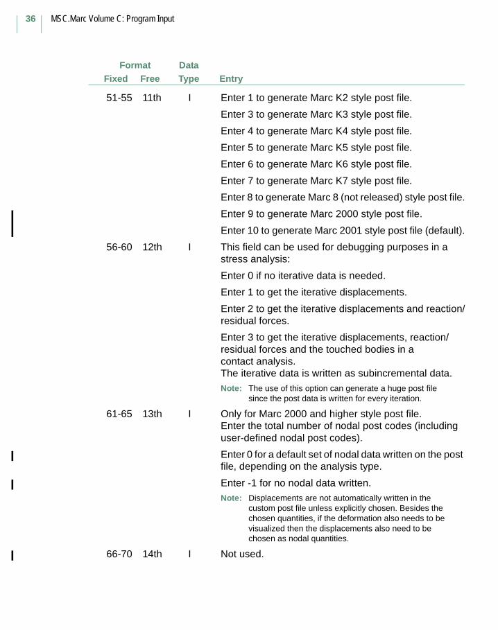
MSC.Marc Volume C: Program Input
36
FormatFree Entry
DataTypeFixed
51-55 11th I Enter 1 to generate Marc K2 style post file.
Enter 3 to generate Marc K3 style post file.
Enter 4 to generate Marc K4 style post file.
Enter 5 to generate Marc K5 style post file.
Enter 6 to generate Marc K6 style post file.
Enter 7 to generate Marc K7 style post file.
Enter 8 to generate Marc 8 (not released) style post file.
Enter 9 to generate Marc 2000 style post file.
Enter 10 to generate Marc 2001 style post file (default).
56-60 12th I This field can be used for debugging purposes in a stress analysis:
Enter 0 if no iterative data is needed.
Enter 1 to get the iterative displacements.
Enter 2 to get the iterative displacements and reaction/residual forces.
Enter 3 to get the iterative displacements, reaction/residual forces and the touched bodies in a contact analysis. The iterative data is written as subincremental data.Note: The use of this option can generate a huge post file
since the post data is written for every iteration.
61-65 13th I Only for Marc 2000 and higher style post file. Enter the total number of nodal post codes (including user-defined nodal post codes).
Enter 0 for a default set of nodal data written on the post file, depending on the analysis type.
Enter -1 for no nodal data written.Note: Displacements are not automatically written in the
custom post file unless explicitly chosen. Besides the chosen quantities, if the deformation also needs to be visualized then the displacements also need to be chosen as nodal quantities.
66-70 14th I Not used.
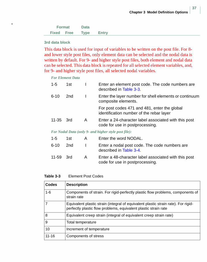
Chapter 3 Model Definition Options37
FormatFree Entry
DataTypeFixed
3rd data block
This data block is used for input of variables to be written on the post file. For 8- and lower style post files, only element data can be selected and the nodal data is written by default. For 9- and higher style post files, both element and nodal data can be selected. This data block is repeated for all selected element variables, and, for 9- and higher style post files, all selected nodal variables.
For Element Data
1-5 1st I Enter an element post code. The code numbers are described in Table 3-3.
6-10 2nd I Enter the layer number for shell elements or continuum composite elements.
For post codes 471 and 481, enter the global identification number of the rebar layer
11-35 3rd A Enter a 24-character label associated with this post code for use in postprocessing.
For Nodal Data (only 9- and higher style post file):
1-5 1st A Enter the word NODAL.
6-10 2nd I Enter a nodal post code. The code numbers are described in Table 3-4.
11-59 3rd A Enter a 48-character label associated with this post code for use in postprocessing.
Table 3-3 Element Post Codes
Codes Description
1-6 Components of strain. For rigid-perfectly plastic flow problems, components of strain rate
7 Equivalent plastic strain (integral of equivalent plastic strain rate). For rigid-perfectly plastic flow problems, equivalent plastic strain rate
8 Equivalent creep strain (integral of equivalent creep strain rate)
9 Total temperature
10 Increment of temperature
11-16 Components of stress
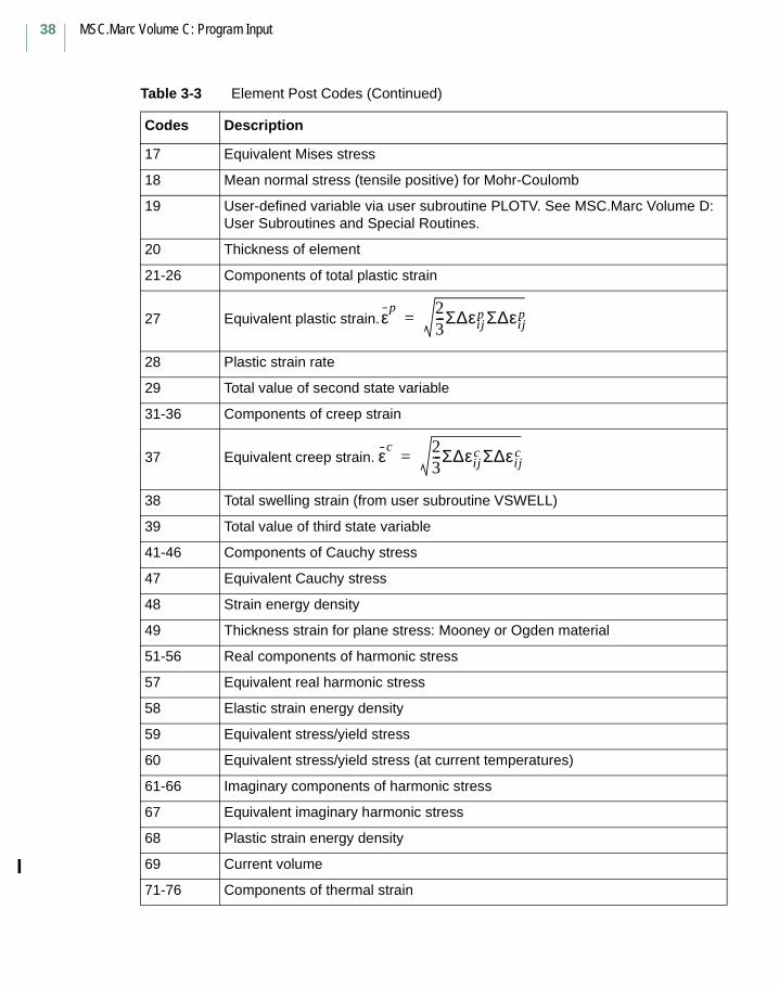
MSC.Marc Volume C: Program Input
38
17 Equivalent Mises stress
18 Mean normal stress (tensile positive) for Mohr-Coulomb
19 User-defined variable via user subroutine PLOTV. See MSC.Marc Volume D: User Subroutines and Special Routines.
20 Thickness of element
21-26 Components of total plastic strain
27 Equivalent plastic strain.
28 Plastic strain rate
29 Total value of second state variable
31-36 Components of creep strain
37 Equivalent creep strain.
38 Total swelling strain (from user subroutine VSWELL)
39 Total value of third state variable
41-46 Components of Cauchy stress
47 Equivalent Cauchy stress
48 Strain energy density
49 Thickness strain for plane stress: Mooney or Ogden material
51-56 Real components of harmonic stress
57 Equivalent real harmonic stress
58 Elastic strain energy density
59 Equivalent stress/yield stress
60 Equivalent stress/yield stress (at current temperatures)
61-66 Imaginary components of harmonic stress
67 Equivalent imaginary harmonic stress
68 Plastic strain energy density
69 Current volume
71-76 Components of thermal strain
Table 3-3 Element Post Codes (Continued)
Codes Description
εp 2
3---Σ∆εij
p Σ∆εijp=
εc 23---Σ∆εij
c Σ∆εijc=
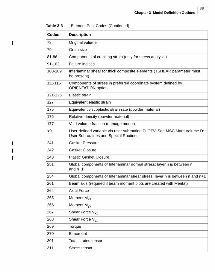
Chapter 3 Model Definition Options39
78 Original volume
79 Grain size
81-86 Components of cracking strain (only for stress analysis)
91-103 Failure indices
108-109 Interlaminar shear for thick composite elements (TSHEAR parameter must be present)
111-116 Components of stress in preferred coordinate system defined by ORIENTATION option
121-126 Elastic strain
127 Equivalent elastic strain
175 Equivalent viscoplastic strain rate (powder material)
176 Relative density (powder material)
177 Void volume fraction (damage model)
<0 User-defined variable via user subroutine PLOTV. See MSC.Marc Volume D: User Subroutines and Special Routines.
241 Gasket Pressure.
242 Gasket Closure.
243 Plastic Gasket Closure.
251 Global components of Interlaminar normal stress; layer n is between n and n+1
254 Global components of Interlaminar shear stress; layer n is between n and n+1
261 Beam axis (required if beam moment plots are created with Mentat)
264 Axial Force
265 Moment Mxx
266 Moment Myy
267 Shear Force Vxz
268 Shear Force Vyz
269 Torque
270 Bimoment
301 Total strains tensor
311 Stress tensor
Table 3-3 Element Post Codes (Continued)
Codes Description
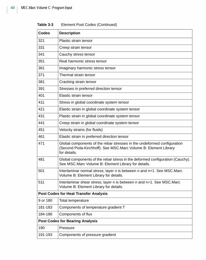
MSC.Marc Volume C: Program Input
40
321 Plastic strain tensor
331 Creep strain tensor
341 Cauchy stress tensor
351 Real harmonic stress tensor
361 Imaginary harmonic stress tensor
371 Thermal strain tensor
381 Cracking strain tensor
391 Stresses in preferred direction tensor
401 Elastic strain tensor
411 Stress in global coordinate system tensor
421 Elastic strain in global coordinate system tensor
431 Plastic strain in global coordinate system tensor
441 Creep strain in global coordinate system tensor
451 Velocity strains (for fluids)
461 Elastic strain in preferred direction tensor
471 Global components of the rebar stresses in the undeformed configuration (Second Piola-Kirchhoff). See MSC.Marc Volume B: Element Library for details.
481 Global components of the rebar stress in the deformed configuration (Cauchy). See MSC.Marc Volume B: Element Library for details.
501 Interlaminar normal stress; layer n is between n and n+1. See MSC.Marc Volume B: Element Library for details.
511 Interlaminar shear stress; layer n is between n and n+1. See MSC.Marc Volume B: Element Library for details.
Post Codes for Heat Transfer Analysis
9 or 180 Total temperature
181-183 Components of temperature gradient T
184-186 Components of flux
Post Codes for Bearing Analysis
190 Pressure
191-193 Components of pressure gradient
Table 3-3 Element Post Codes (Continued)
Codes Description
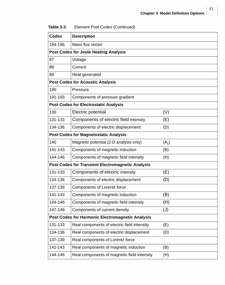
Chapter 3 Model Definition Options41
194-196 Mass flux vector
Post Codes for Joule Heating Analysis
87 Voltage
88 Current
89 Heat generated
Post Codes for Acoustic Analysis
190 Pressure
191-193 Components of pressure gradient
Post Codes for Electrostatic Analysis
130 Electric potential (V)
131-133 Components of electric field intensity (E)
134-136 Components of electric displacement (D)
Post Codes for Magnetostatic Analysis
140 Magnetic potential (2-D analysis only) (Az)
141-143 Components of magnetic induction (B)
144-146 Components of magnetic field intensity (H)
Post Codes for Transient Electromagnetic Analysis
131-133 Components of electric intensity (E)
134-136 Components of electric displacement (D)
137-139 Components of Lorentz force
141-143 Components of magnetic induction (B)
144-146 Components of magnetic field intensity (H)
147-149 Components of current density (J)
Post Codes for Harmonic Electromagnetic Analysis
131-133 Real components of electric field intensity (E)
134-136 Real components of electric displacement (D)
137-139 Real components of Lorentz force
141-143 Real components of magnetic induction (B)
144-146 Real components of magnetic field intensity (H)
Table 3-3 Element Post Codes (Continued)
Codes Description

MSC.Marc Volume C: Program Input
42
Notes: Codes 1-6 are the generalized strains and are section (not layer) quantities, so that the layer number need not be given.
Codes 11-16 give generalized stress quantities if no layer number is given for shell analysis. If a layer number is given, these are physical layer quantities.
For heat transfer, code 9 is used for all heat transfer elements.
When using shells in heat transfer, it is important to enter a code for each layer in chronological order if post file is to be correctly read by the INITIAL STATE or CHANGE STATE options.
Note that you do not need to select nodal values (that is, displacement, velocities and accelerations, and temperature for a heat transfer run) as these are automatically written to the post file.
Eigenmodes (dynamic analysis) and eigenvectors (buckling analysis) are written to the post file only if indicated by the RECOVER or MODAL INCREMENT/BUCKLE INCREMENT option.
For post codes 411, 421, 431, and 441 global quantities for shell elements are reported for as many layers and use the same layer numbering system as regular shell quantities. Layer 1 is the top surface; layer 2 is the next surface, etc. This convention is followed from Marc 2000 on.
147-149 Real components of current density (J)
151-153 Imaginary components of electric field intensity (E)
154-156 Imaginary components of electric displacement (D)
157-159 Imaginary components of Lorentz force
161-163 Imaginary components of magnetic induction (B)
164-166 Imaginary components of magnetic field intensity (H)
167-169 Imaginary components of current density (J)
Post Codes for Soil Analysis
171 Porosity
172 Void ratio
173 Pore pressure
174 Preconsolidation pressure
Table 3-3 Element Post Codes (Continued)
Codes Description
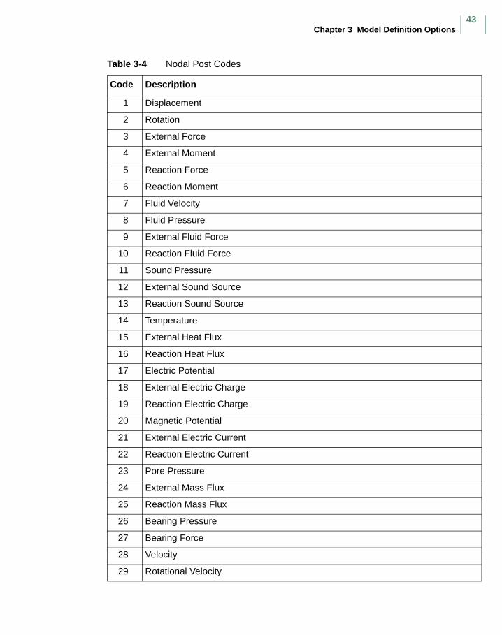
Chapter 3 Model Definition Options43
Table 3-4 Nodal Post Codes
Code Description
1 Displacement
2 Rotation
3 External Force
4 External Moment
5 Reaction Force
6 Reaction Moment
7 Fluid Velocity
8 Fluid Pressure
9 External Fluid Force
10 Reaction Fluid Force
11 Sound Pressure
12 External Sound Source
13 Reaction Sound Source
14 Temperature
15 External Heat Flux
16 Reaction Heat Flux
17 Electric Potential
18 External Electric Charge
19 Reaction Electric Charge
20 Magnetic Potential
21 External Electric Current
22 Reaction Electric Current
23 Pore Pressure
24 External Mass Flux
25 Reaction Mass Flux
26 Bearing Pressure
27 Bearing Force
28 Velocity
29 Rotational Velocity

MSC.Marc Volume C: Program Input
44
30 Acceleration
31 Rotational Acceleration
32 Modal Mass
33 Rotational Modal Mass
34 Contact Normal Stress
35 Contact Normal Force
36 Contact Friction Stress
37 Contact Friction Force
38 Contact Status
39 Contact Touched Body
40 Herrmann Variable
<0 User-defined nodal quantity via user subroutine UPSTNO.
Table 3-4 Nodal Post Codes
Code Description

Chapter 3 Model Definition Options45
INITIAL PLASTIC STRAIN
Define Initial Plastic Strain
Description
This option provides various ways of initializing the equivalent plastic strain throughout the model. Occasionally, in metal forming analysis, it is required to define the previous amount of equivalent plastic strain. This history dependent variable represents the amount of plastic deformation that the model was subjected to, and is used in the work (strain) hardening model.
Four ways of specifying the initial equivalent plastic strain values are shown below:
• Read the range of elements, integration points and layers and a corresponding value.
• Read the initial values through user subroutine INITPL.
• Read the initial values from a step of the post output file from a previous analysis with Marc. With this option, Marc assumes direct correspondence of the post file elements with the elements in the current analysis. Any spatial interpolation must be provided separately by you.
• Read a list of elements, integration points and layers and a corresponding value.
FormatFree Entry
DataTypeFixed
Format
1st data block
1-13 1st A Enter the words INITIAL PLASTIC STRAIN.
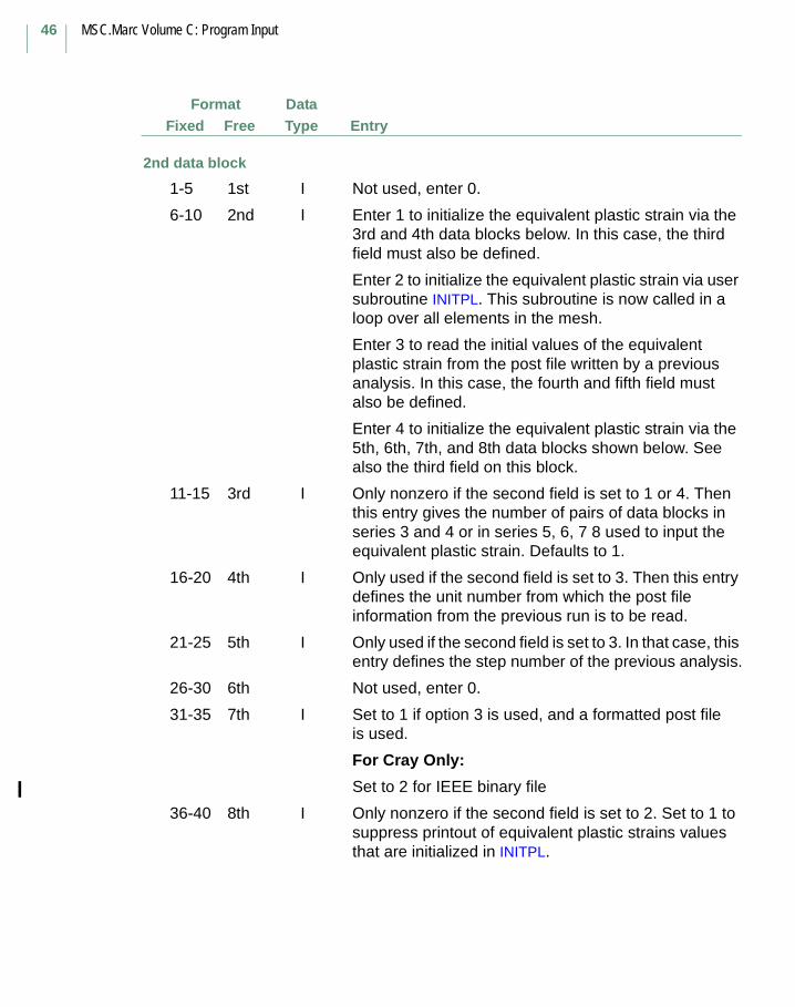
MSC.Marc Volume C: Program Input
46
FormatFree Entry
DataTypeFixed
2nd data block
1-5 1st I Not used, enter 0.
6-10 2nd I Enter 1 to initialize the equivalent plastic strain via the 3rd and 4th data blocks below. In this case, the third field must also be defined.
Enter 2 to initialize the equivalent plastic strain via user subroutine INITPL. This subroutine is now called in a loop over all elements in the mesh.
Enter 3 to read the initial values of the equivalent plastic strain from the post file written by a previous analysis. In this case, the fourth and fifth field must also be defined.
Enter 4 to initialize the equivalent plastic strain via the 5th, 6th, 7th, and 8th data blocks shown below. See also the third field on this block.
11-15 3rd I Only nonzero if the second field is set to 1 or 4. Then this entry gives the number of pairs of data blocks in series 3 and 4 or in series 5, 6, 7 8 used to input the equivalent plastic strain. Defaults to 1.
16-20 4th I Only used if the second field is set to 3. Then this entry defines the unit number from which the post file information from the previous run is to be read.
21-25 5th I Only used if the second field is set to 3. In that case, this entry defines the step number of the previous analysis.
26-30 6th Not used, enter 0.
31-35 7th I Set to 1 if option 3 is used, and a formatted post file is used.
For Cray Only:
Set to 2 for IEEE binary file
36-40 8th I Only nonzero if the second field is set to 2. Set to 1 to suppress printout of equivalent plastic strains values that are initialized in INITPL.
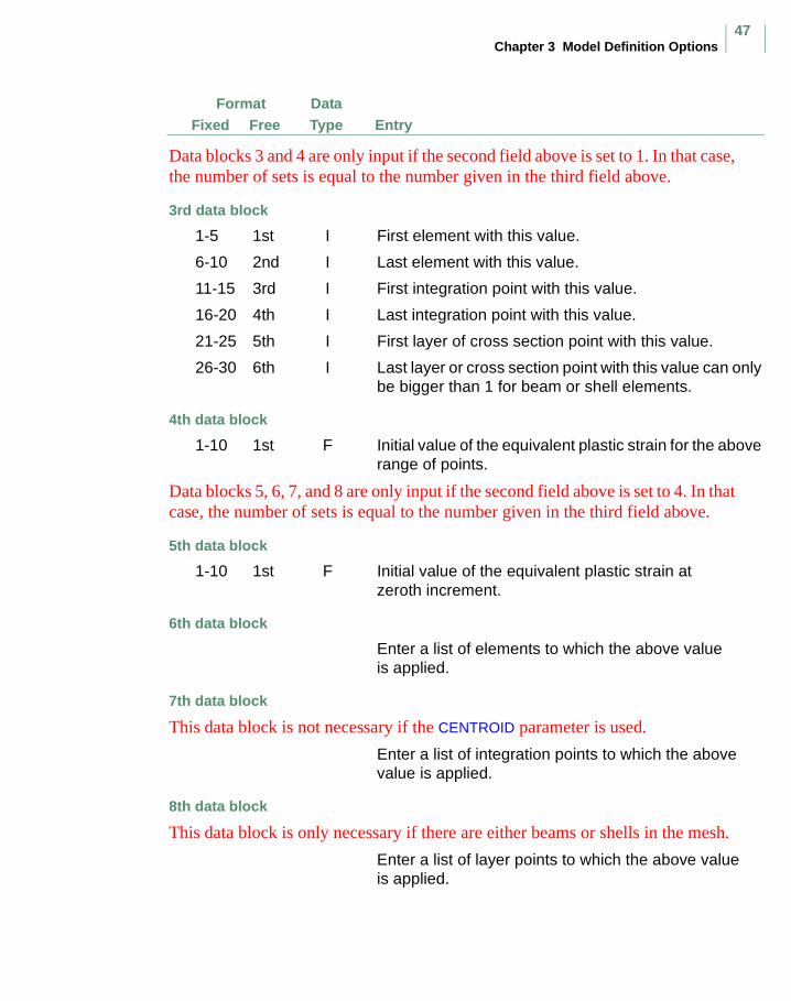
Chapter 3 Model Definition Options47
FormatFree Entry
DataTypeFixed
Data blocks 3 and 4 are only input if the second field above is set to 1. In that case, the number of sets is equal to the number given in the third field above.
3rd data block
1-5 1st I First element with this value.
6-10 2nd I Last element with this value.
11-15 3rd I First integration point with this value.
16-20 4th I Last integration point with this value.
21-25 5th I First layer of cross section point with this value.
26-30 6th I Last layer or cross section point with this value can only be bigger than 1 for beam or shell elements.
4th data block
1-10 1st F Initial value of the equivalent plastic strain for the above range of points.
Data blocks 5, 6, 7, and 8 are only input if the second field above is set to 4. In that case, the number of sets is equal to the number given in the third field above.
5th data block
1-10 1st F Initial value of the equivalent plastic strain at zeroth increment.
6th data block
Enter a list of elements to which the above value is applied.
7th data block
This data block is not necessary if the CENTROID parameter is used.
Enter a list of integration points to which the above value is applied.
8th data block
This data block is only necessary if there are either beams or shells in the mesh.
Enter a list of layer points to which the above value is applied.

MSC.Marc Volume C: Program Input
48
INITIAL STATE
Initialize State Variables
Description
This option provides various ways of initializing the state variables throughout the model. The number of state variables per integration point is defined in the STATE VARS parameter. The default is one, with temperature always being the first state variable at an integration point. If more than one state variable per integration point has been assigned, this option can be used repeatedly to initialize all the state variables. The default value of state variables not initialized is zero.
Four ways of providing the state variable initial values are shown below:
• Read the range of elements, integration points and layers and a corresponding state variable value.
• Read the initial values through user subroutine INITSV.
• Read the initial values from a step of the binary or formatted post output file from a previous heat transfer analysis with Marc. This technique is most common for thermal stress analysis to initialize temperature (the first state variable at any point). With this option Marc assumes direct correspondence of the post file elements with the elements in the current analysis. Any spatial interpolation must be provided separately by you.
• Read a list of elements, integration points and layers and a corresponding state variable value.
Note: Initial temperature values read in by this option are assumed to define the stress-free temperature field. Temperature changes which cause thermal strains are read in through the CHANGE STATE or AUTO THERM options.
In a coupled analysis, the temperatures are not independent state variables and the INITIAL TEMP option must be used.

Chapter 3 Model Definition Options49
FormatFree Entry
DataTypeFixed
1st data block
1-13 1st A Enter the words INITIAL STATE.
2nd data block
1-5 1st I Enter the state variable identifier for the state variable being set (1,2,etc.). 1=temperature. If more than one state variable is being used, the STATE VARS parameter must be included.
6-10 2nd I Enter 1 to initialize the state variable via the 3rd and 4th data block below. See also the third field on this data block.
Enter 2 to initialize the state variable via user subroutine INITSV. This subroutine is now called in a loop over all elements in the mesh.
Enter 3 to read the file values of the state variable from the post file written by a previous heat transfer analysis. In this case, the fourth and fifth fields must also be defined.
Enter 4 to initialize the state variable via the 5th, 6th, 7th, and 8th data blocks as given below. Also, see the third field on this data block.
11-15 3rd I Only nonzero if the second field is set to 1 or 4. Then this entry gives the number of pairs of data blocks in series 3 and 4 or in series 5, 6, 7, and 8 used to input the state variable.
16-20 4th I Only used if the second field is set to 3. Then this entry defines the unit number from which the post file information from the previous heat transfer run is to be read. Defaults to unit 24 for a formatted post file and to unit 25 for a binary post file.
21-25 5th I Only used if the second field is set to 3. In that case, this entry defines the increment number on the heat transfer run post file to be used as the definition of the initial state variable values.
26-30 6th Not used, enter 0.
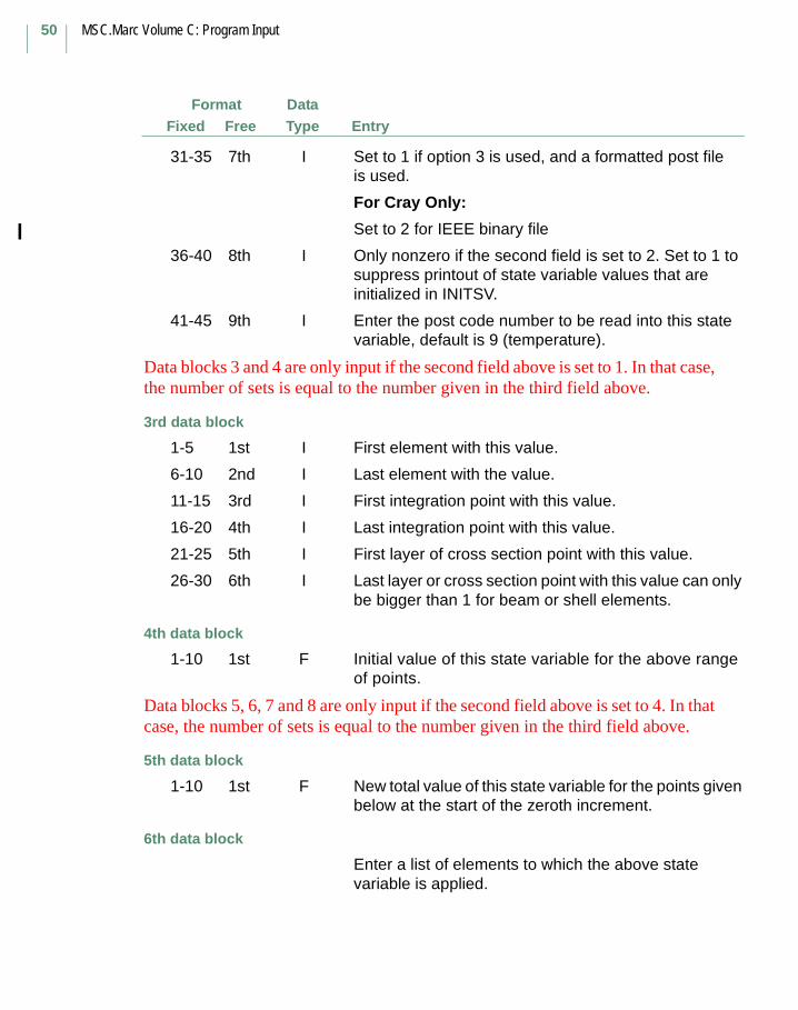
MSC.Marc Volume C: Program Input
50
FormatFree Entry
DataTypeFixed
31-35 7th I Set to 1 if option 3 is used, and a formatted post file is used.
For Cray Only:
Set to 2 for IEEE binary file
36-40 8th I Only nonzero if the second field is set to 2. Set to 1 to suppress printout of state variable values that are initialized in INITSV.
41-45 9th I Enter the post code number to be read into this state variable, default is 9 (temperature).
Data blocks 3 and 4 are only input if the second field above is set to 1. In that case, the number of sets is equal to the number given in the third field above.
3rd data block
1-5 1st I First element with this value.
6-10 2nd I Last element with the value.
11-15 3rd I First integration point with this value.
16-20 4th I Last integration point with this value.
21-25 5th I First layer of cross section point with this value.
26-30 6th I Last layer or cross section point with this value can only be bigger than 1 for beam or shell elements.
4th data block
1-10 1st F Initial value of this state variable for the above range of points.
Data blocks 5, 6, 7 and 8 are only input if the second field above is set to 4. In that case, the number of sets is equal to the number given in the third field above.
5th data block
1-10 1st F New total value of this state variable for the points given below at the start of the zeroth increment.
6th data block
Enter a list of elements to which the above state variable is applied.

Chapter 3 Model Definition Options51
FormatFree Entry
DataTypeFixed
7th data block
This data block is not necessary if the CENTROID parameter is used.
Enter a list of integration points to which the above state variable is applied.
8th data block
This data block is only necessary if there are either beams or shells in the mesh.
Enter a list of layer points to which the above state variable is applied.
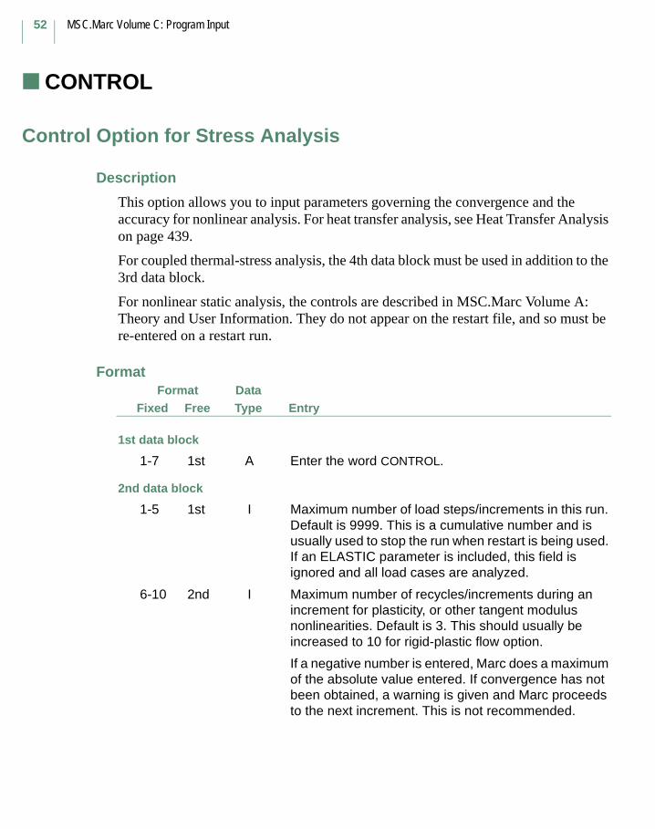
MSC.Marc Volume C: Program Input
52
CONTROL (Mechanical)
Control Option for Stress Analysis
Description
This option allows you to input parameters governing the convergence and the accuracy for nonlinear analysis. For heat transfer analysis, see Heat Transfer Analysis on page 439.
For coupled thermal-stress analysis, the 4th data block must be used in addition to the 3rd data block.
For nonlinear static analysis, the controls are described in MSC.Marc Volume A: Theory and User Information. They do not appear on the restart file, and so must be re-entered on a restart run.
FormatFree Entry
DataTypeFixed
Format
1st data block
1-7 1st A Enter the word CONTROL.
2nd data block
1-5 1st I Maximum number of load steps/increments in this run. Default is 9999. This is a cumulative number and is usually used to stop the run when restart is being used. If an ELASTIC parameter is included, this field is ignored and all load cases are analyzed.
6-10 2nd I Maximum number of recycles/increments during an increment for plasticity, or other tangent modulus nonlinearities. Default is 3. This should usually be increased to 10 for rigid-plastic flow option.
If a negative number is entered, Marc does a maximum of the absolute value entered. If convergence has not been obtained, a warning is given and Marc proceeds to the next increment. This is not recommended.
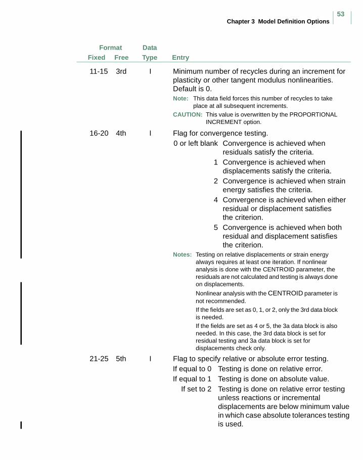
Chapter 3 Model Definition Options53
FormatFree Entry
DataTypeFixed
11-15 3rd I Minimum number of recycles during an increment for plasticity or other tangent modulus nonlinearities. Default is 0. Note: This data field forces this number of recycles to take
place at all subsequent increments.CAUTION: This value is overwritten by the PROPORTIONAL
INCREMENT option.
16-20 4th I Flag for convergence testing. 0 or left blank Convergence is achieved when
residuals satisfy the criteria. 1 Convergence is achieved when
displacements satisfy the criteria.2 Convergence is achieved when strain
energy satisfies the criteria.4 Convergence is achieved when either
residual or displacement satisfies the criterion.
5 Convergence is achieved when both residual and displacement satisfies the criterion.
Notes: Testing on relative displacements or strain energy always requires at least one iteration. If nonlinear analysis is done with the CENTROID parameter, the residuals are not calculated and testing is always done on displacements.
Nonlinear analysis with the CENTROID parameter is not recommended. If the fields are set as 0, 1, or 2, only the 3rd data block is needed.If the fields are set as 4 or 5, the 3a data block is also needed. In this case, the 3rd data block is set for residual testing and 3a data block is set for displacements check only.
21-25 5th I Flag to specify relative or absolute error testing.If equal to 0 Testing is done on relative error.If equal to 1 Testing is done on absolute value.
If set to 2 Testing is done on relative error testing unless reactions or incremental displacements are below minimum value in which case absolute tolerances testing is used.
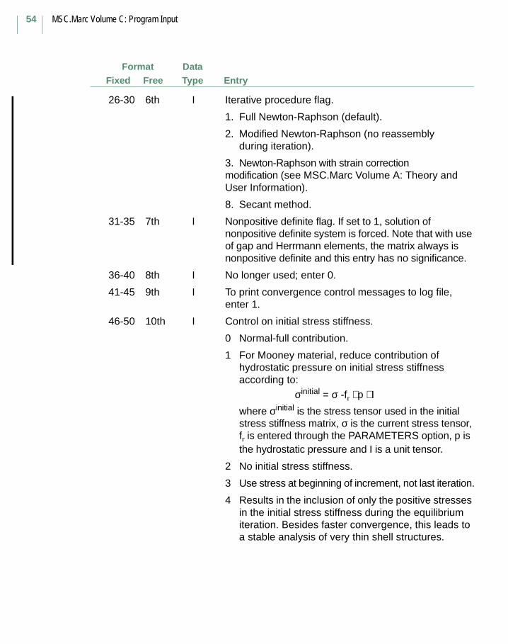
MSC.Marc Volume C: Program Input
54
FormatFree Entry
DataTypeFixed
26-30 6th I Iterative procedure flag.
1. Full Newton-Raphson (default).
2. Modified Newton-Raphson (no reassembly during iteration).
3. Newton-Raphson with strain correction modification (see MSC.Marc Volume A: Theory and User Information).
8. Secant method.
31-35 7th I Nonpositive definite flag. If set to 1, solution of nonpositive definite system is forced. Note that with use of gap and Herrmann elements, the matrix always is nonpositive definite and this entry has no significance.
36-40 8th I No longer used; enter 0.
41-45 9th I To print convergence control messages to log file, enter 1.
46-50 10th I Control on initial stress stiffness.
0 Normal-full contribution.
1 For Mooney material, reduce contribution of hydrostatic pressure on initial stress stiffness according to:
σinitial = σ -fr ⋅ p ⋅ Iwhere σinitial is the stress tensor used in the initial stress stiffness matrix, σ is the current stress tensor, fr is entered through the PARAMETERS option, p is the hydrostatic pressure and I is a unit tensor.
2 No initial stress stiffness.
3 Use stress at beginning of increment, not last iteration.
4 Results in the inclusion of only the positive stresses in the initial stress stiffness during the equilibrium iteration. Besides faster convergence, this leads to a stable analysis of very thin shell structures.
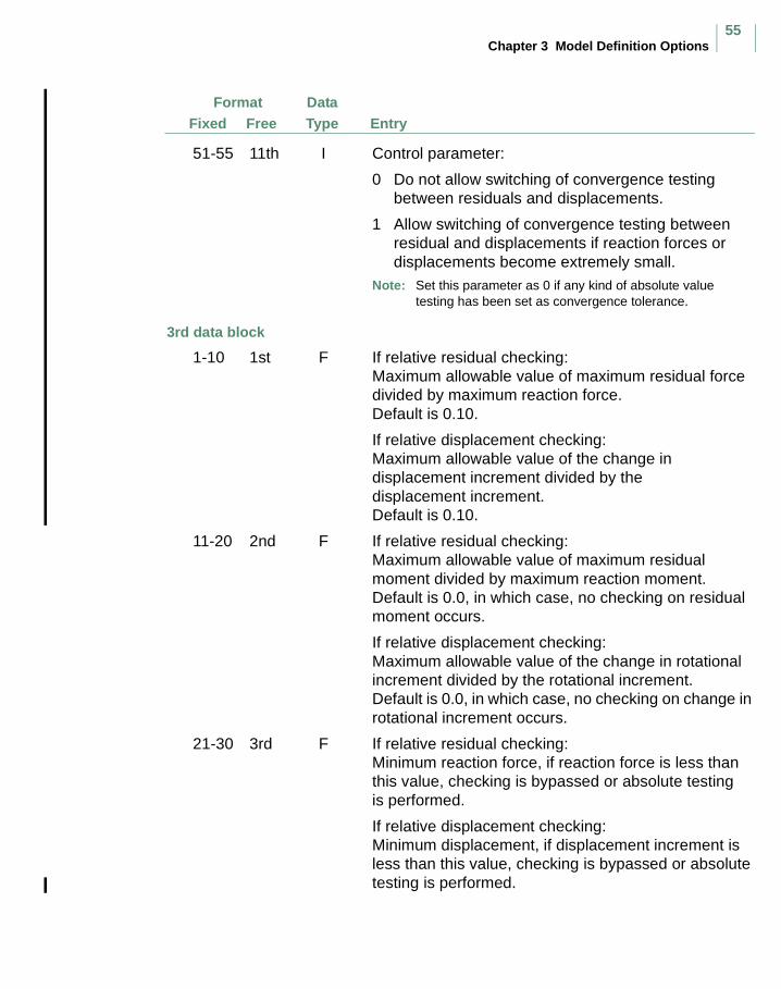
Chapter 3 Model Definition Options55
FormatFree Entry
DataTypeFixed
51-55 11th I Control parameter:
0 Do not allow switching of convergence testing between residuals and displacements.
1 Allow switching of convergence testing between residual and displacements if reaction forces or displacements become extremely small.
Note: Set this parameter as 0 if any kind of absolute value testing has been set as convergence tolerance.
3rd data block
1-10 1st F If relative residual checking: Maximum allowable value of maximum residual force divided by maximum reaction force. Default is 0.10.
If relative displacement checking: Maximum allowable value of the change in displacement increment divided by the displacement increment. Default is 0.10.
11-20 2nd F If relative residual checking: Maximum allowable value of maximum residual moment divided by maximum reaction moment. Default is 0.0, in which case, no checking on residual moment occurs.
If relative displacement checking: Maximum allowable value of the change in rotational increment divided by the rotational increment. Default is 0.0, in which case, no checking on change in rotational increment occurs.
21-30 3rd F If relative residual checking: Minimum reaction force, if reaction force is less than this value, checking is bypassed or absolute testing is performed.
If relative displacement checking: Minimum displacement, if displacement increment is less than this value, checking is bypassed or absolute testing is performed.
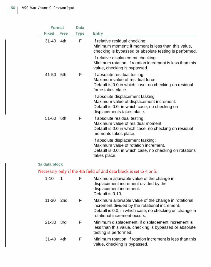
MSC.Marc Volume C: Program Input
56
FormatFree Entry
DataTypeFixed
31-40 4th F If relative residual checking: Minimum moment: if moment is less than this value, checking is bypassed or absolute testing is performed.
If relative displacement checking: Minimum rotation: if rotation increment is less than this value, checking is bypassed.
41-50 5th F If absolute residual testing:Maximum value of residual force. Default is 0.0 in which case, no checking on residual force takes place.
If absolute displacement taskingMaximum value of displacement increment.Default is 0.0; in which case, no checking on displacements takes place.
51-60 6th F If absolute residual testing:Maximum value of residual moment. Default is 0.0 in which case, no checking on residual moments takes place.
If absolute displacement tasking:Maximum value of rotation increment.Default is 0.0; in which case, no checking on rotations takes place.
3a data block
Necessary only if the 4th field of 2nd data block is set to 4 or 5.
1-10 1 F Maximum allowable value of the change in displacement increment divided by the displacement increment. Default is 0.10.
11-20 2nd F Maximum allowable value of the change in rotational increment divided by the rotational increment. Default is 0.0, in which case, no checking on change in rotational increment occurs.
21-30 3rd F Minimum displacement, if displacement increment is less than this value, checking is bypassed or absolute testing is performed.
31-40 4th F Minimum rotation: if rotation increment is less than this value, checking is bypassed.
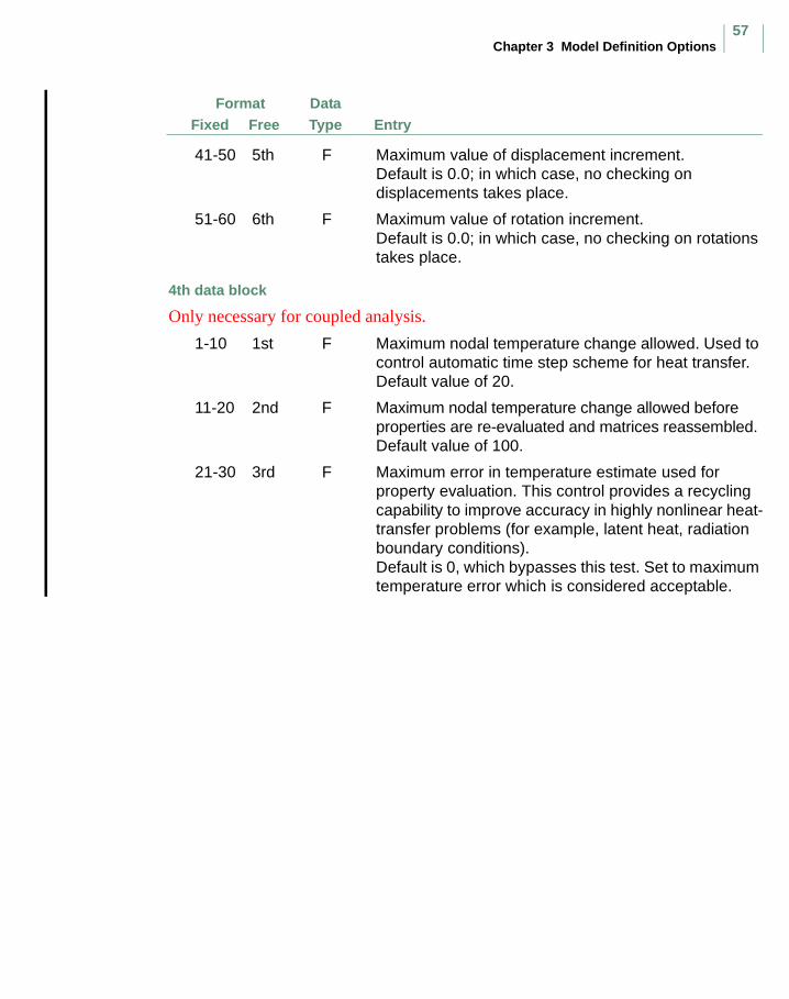
Chapter 3 Model Definition Options57
FormatFree Entry
DataTypeFixed
41-50 5th F Maximum value of displacement increment.Default is 0.0; in which case, no checking on displacements takes place.
51-60 6th F Maximum value of rotation increment.Default is 0.0; in which case, no checking on rotations takes place.
4th data block
Only necessary for coupled analysis.
1-10 1st F Maximum nodal temperature change allowed. Used to control automatic time step scheme for heat transfer. Default value of 20.
11-20 2nd F Maximum nodal temperature change allowed before properties are re-evaluated and matrices reassembled. Default value of 100.
21-30 3rd F Maximum error in temperature estimate used for property evaluation. This control provides a recycling capability to improve accuracy in highly nonlinear heat-transfer problems (for example, latent heat, radiation boundary conditions). Default is 0, which bypasses this test. Set to maximum temperature error which is considered acceptable.
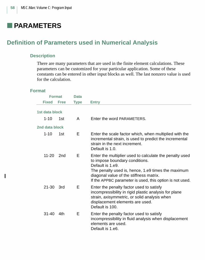
MSC.Marc Volume C: Program Input
58
PARAMETERS (Model Definition)
Definition of Parameters used in Numerical Analysis
Description
There are many parameters that are used in the finite element calculations. These parameters can be customized for your particular application. Some of these constants can be entered in other input blocks as well. The last nonzero value is used for the calculation.
FormatFree Entry
DataTypeFixed
Format
1st data block
1-10 1st A Enter the word PARAMETERS.
2nd data block
1-10 1st E Enter the scale factor which, when multiplied with the incremental strain, is used to predict the incremental strain in the next increment.Default is 1.0.
11-20 2nd E Enter the multiplier used to calculate the penalty used to impose boundary conditions.Default is 1.e9.The penalty used is, hence, 1.e9 times the maximum diagonal value of the stiffness matrix. If the APPBC parameter is used, this option is not used.
21-30 3rd E Enter the penalty factor used to satisfy incompressibility in rigid plastic analysis for plane strain, axisymmetric, or solid analysis when displacement elements are used.Default is 100.
31-40 4th E Enter the penalty factor used to satisfy incompressibility in fluid analysis when displacement elements are used.Default is 1.e6.
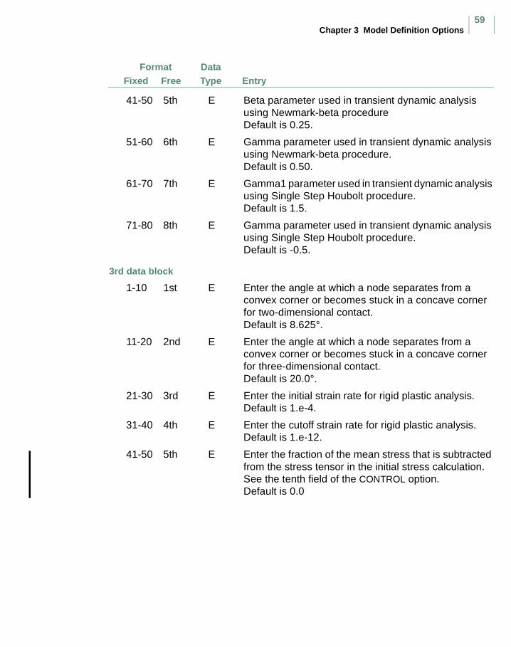
Chapter 3 Model Definition Options59
FormatFree Entry
DataTypeFixed
41-50 5th E Beta parameter used in transient dynamic analysis using Newmark-beta procedureDefault is 0.25.
51-60 6th E Gamma parameter used in transient dynamic analysis using Newmark-beta procedure.Default is 0.50.
61-70 7th E Gamma1 parameter used in transient dynamic analysis using Single Step Houbolt procedure.Default is 1.5.
71-80 8th E Gamma parameter used in transient dynamic analysis using Single Step Houbolt procedure.Default is -0.5.
3rd data block
1-10 1st E Enter the angle at which a node separates from a convex corner or becomes stuck in a concave corner for two-dimensional contact.Default is 8.625°.
11-20 2nd E Enter the angle at which a node separates from a convex corner or becomes stuck in a concave corner for three-dimensional contact.Default is 20.0°.
21-30 3rd E Enter the initial strain rate for rigid plastic analysis.Default is 1.e-4.
31-40 4th E Enter the cutoff strain rate for rigid plastic analysis.Default is 1.e-12.
41-50 5th E Enter the fraction of the mean stress that is subtracted from the stress tensor in the initial stress calculation. See the tenth field of the CONTROL option.Default is 0.0
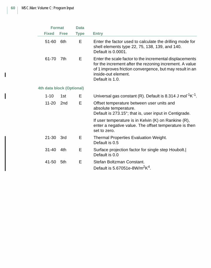
MSC.Marc Volume C: Program Input
60
FormatFree Entry
DataTypeFixed
51-60 6th E Enter the factor used to calculate the drilling mode for shell elements type 22, 75, 138, 139, and 140.Default is 0.0001.
61-70 7th E Enter the scale factor to the incremental displacements for the increment after the rezoning increment. A value of 1 improves friction convergence, but may result in an inside-out element. Default is 1.0.
4th data block (Optional)
1-10 1st E Universal gas constant (R). Default is 8.314 J mol-1K-1.
11-20 2nd E Offset temperature between user units and absolute temperature. Default is 273.15°; that is, user input in Centigrade.
If user temperature is in Kelvin (K) on Rankine (R), enter a negative value. The offset temperature is then set to zero.
21-30 3rd E Thermal Properties Evaluation Weight.Default is 0.5
31-40 4th E Surface projection factor for single step Houbolt.|Default is 0.0
41-50 5th E Stefan Boltzman Constant.
Default is 5.67051e-8W/m2K4.
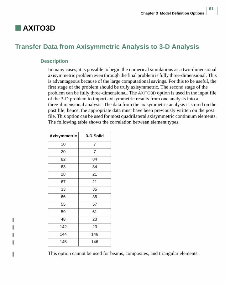
Chapter 3 Model Definition Options61
AXITO3D (Model Definition)
Transfer Data from Axisymmetric Analysis to 3-D Analysis
Description
In many cases, it is possible to begin the numerical simulations as a two-dimensional axisymmetric problem even through the final problem is fully three-dimensional. This is advantageous because of the large computational savings. For this to be useful, the first stage of the problem should be truly axisymmetric. The second stage of the problem can be fully three-dimensional. The AXITO3D option is used in the input file of the 3-D problem to import axisymmetric results from one analysis into a three-dimensional analysis. The data from the axisymmetric analysis is stored on the post file; hence, the appropriate data must have been previously written on the post file. This option can be used for most quadrilateral axisymmetric continuum elements. The following table shows the correlation between element types.
This option cannot be used for beams, composites, and triangular elements.
Axisymmetric 3-D Solid
10 7
20 7
82 84
83 84
28 21
67 21
33 35
66 35
55 57
59 61
48 23
142 23
144 146
145 146

MSC.Marc Volume C: Program Input
62
There are three steps required to perform these types of analysis using Mentat.
1. Perform axisymmetric analysis:
a. Create axisymmetric model using Mentat.
b. Save the created model; for example, into stage_axi.mud.
c. Run axisymmetric model and keep post file (stage_axi_job1.t16 or stage_axi_job1.t19).
Note: Make certain that the post file contains the data to be transferred. For example, for metal plasticity using PLASTICITY,3, this would include at least stress (post code 311) and equivalent plastic strain (post code 7). For rubber elasticity using ELASTICITY,2, strain (post code 301) and stress are needed. For analysis involving temperature, post code 9 is required. Creep strain and equivalent creep strain, velocity and acceleration are needed for creep and dynamic analysis, respectively.
2. Create 3-D model using Mentat.
a. Open axisymmetric model stage_axi.mud.
b. Expand axisymmetric mesh to 3-D model via:
MESH GENERATION⇒ EXPAND⇒ AXSYMMETRIC MODEL TO 3D
and move the rigid surfaces, if any, to the deformed configuration.
c. Define data transfer parameters via:
INITIAL CONDITIONS⇒ MECHANICAL⇒ AXSYMMETRIC-3D
d. Add additional model data such as contact surfaces if necessary.
e. Save the created model with a different name to avoid overwriting the existing stage_axi.mud; for example, into stage_3d.mud.
3. Run 3-D model.
Note: (1) If a 3-D analysis is run outside of Mentat, use the -pid command line option to read in a post file of axisymmetric analysis. For example, to submit a 3-D analysis, use the command:
marc -j stage_3d_job1 -pid stage_axi_job1
(2) If remeshing/rezoning steps are performed in the axisymmetric analysis, the original mesh in the model is replaced by a new mesh. The 3-D analysis starts based on the deformed configuration.
To replace step 2-a above, do the following:
i. Open post file stage_axi.t16 (or stage_axi.t19)ii. Position to the desired increment.iii. Rezone.iv. Save the model to stage_3d.mud.v. Close post file.
vi. Open stage_3d.mud.
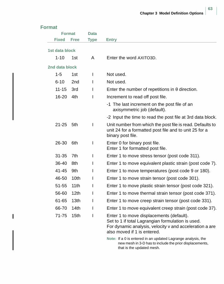
Chapter 3 Model Definition Options63
FormatFree Entry
DataTypeFixed
Format
1st data block
1-10 1st A Enter the word AXITO3D.
2nd data block
1-5 1st I Not used.
6-10 2nd I Not used.
11-15 3rd I Enter the number of repetitions in θ direction.
16-20 4th I Increment to read off post file.
-1 The last increment on the post file of an axisymmetric job (default).
-2 Input the time to read the post file at 3rd data block.
21-25 5th I Unit number from which the post file is read. Defaults to unit 24 for a formatted post file and to unit 25 for a binary post file.
26-30 6th I Enter 0 for binary post file.Enter 1 for formatted post file.
31-35 7th I Enter 1 to move stress tensor (post code 311).
36-40 8th I Enter 1 to move equivalent plastic strain (post code 7).
41-45 9th I Enter 1 to move temperatures (post code 9 or 180).
46-50 10th I Enter 1 to move strain tensor (post code 301).
51-55 11th I Enter 1 to move plastic strain tensor (post code 321).
56-60 12th I Enter 1 to move thermal strain tensor (post code 371).
61-65 13th I Enter 1 to move creep strain tensor (post code 331).
66-70 14th I Enter 1 to move equivalent creep strain (post code 37).
71-75 15th I Enter 1 to move displacements (default). Set to 1 if total Lagrangian formulation is used.For dynamic analysis, velocity v and acceleration a are also moved if 1 is entered.Note: If a 0 is entered in an updated Lagrange analysis, the
new mesh in 3-D has to include the prior displacements, that is the updated mesh.

MSC.Marc Volume C: Program Input
64
FormatFree Entry
DataTypeFixed
The 3rd data block is needed only if the 4th field of the 2nd data block is -2.
3rd data block
1-10 1st F Enter the time to read the post file.
Default is the last increment in the post file.
Chapter 3 Model Definition Options65
CHANGE STATE (Model Definition)
Redefine State Variables
Description
This option provides various ways of changing the state variables throughout the model. State variables are initialized in the INITIAL STATE model definition set. The number of state variables per point is defined in the STATE VARS parameter. The default is one, with temperature always being the first state variable at a point. If more than one state variable per point has been assigned, this option can be used repeatedly to change the values of all state variables. The default value is no change if this option is not used. In this option, the values of the state variable at the end of the current increment are read in. When the temperature is being defined, the following points should be noted:
• For “history following analysis”, the thermal strains are based on temperature change during this step.
• For elastic re-analysis (ELASTIC parameter) the thermal strains are always based on temperature change between the initial, stress free temperature field and the values read in here.
• The AUTO LOAD option is available for specifying a time-varying history of state variables. The value of the total state variable at the end of each increment is specified.
• The AUTO THERM option is available for automatic control of a nonlinear (elastic-plastic) temperature loaded stress problem, to be used in conjunction with this option.
• The THERMAL LOADS option can be used as an alternate to input the change of temperature. Either incremental or total temperatures can be specified using this option.
• The AUTO THERM CREEP option is available for automatic control of a thermally loaded elastic-plastic-creep problem, to be used in conjunction with this option.
Four ways of changing any state variable through CHANGE STATE are possible:
• Read a range of elements, integration points and layers and a corresponding state variable value for the end of the current step.
• Read the state variable values for the end of the current step through user subroutine NEWSV.
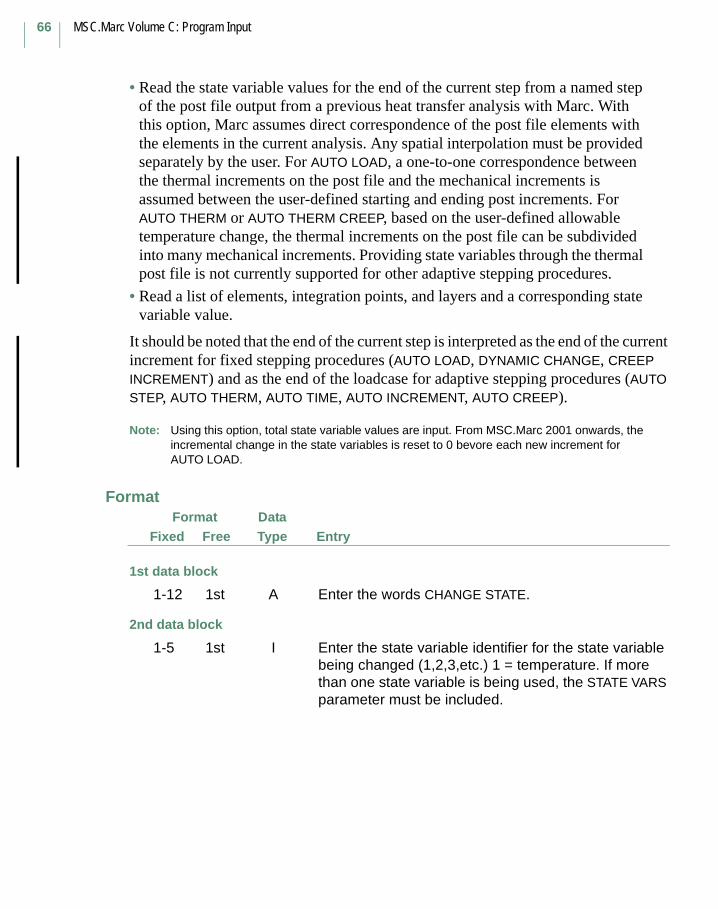
MSC.Marc Volume C: Program Input
66
• Read the state variable values for the end of the current step from a named step of the post file output from a previous heat transfer analysis with Marc. With this option, Marc assumes direct correspondence of the post file elements with the elements in the current analysis. Any spatial interpolation must be provided separately by the user. For AUTO LOAD, a one-to-one correspondence between the thermal increments on the post file and the mechanical increments is assumed between the user-defined starting and ending post increments. For AUTO THERM or AUTO THERM CREEP, based on the user-defined allowable temperature change, the thermal increments on the post file can be subdivided into many mechanical increments. Providing state variables through the thermal post file is not currently supported for other adaptive stepping procedures.
• Read a list of elements, integration points, and layers and a corresponding state variable value.
It should be noted that the end of the current step is interpreted as the end of the current increment for fixed stepping procedures (AUTO LOAD, DYNAMIC CHANGE, CREEP INCREMENT) and as the end of the loadcase for adaptive stepping procedures (AUTO STEP, AUTO THERM, AUTO TIME, AUTO INCREMENT, AUTO CREEP).
Note: Using this option, total state variable values are input. From MSC.Marc 2001 onwards, the incremental change in the state variables is reset to 0 bevore each new increment for AUTO LOAD.
FormatFree Entry
DataTypeFixed
Format
1st data block
1-12 1st A Enter the words CHANGE STATE.
2nd data block
1-5 1st I Enter the state variable identifier for the state variable being changed (1,2,3,etc.) 1 = temperature. If more than one state variable is being used, the STATE VARS parameter must be included.

Chapter 3 Model Definition Options67
FormatFree Entry
DataTypeFixed
6-10 2nd I Enter 1 to change the state variable via the 3rd and 4th data blocks below. In this case, the third field must also be defined.
Enter 2 to change the state variable via user subroutine NEWSV. This subroutine is now called in a loop on all the elements in the mesh.
Enter 3 to read the new values of the state variable from a post file written by a previous heat transfer analysis. In this case, the fourth and fifth field must be defined.
Enter 4 to change the state variable via data blocks 5, 6, 7, and 8 below.
11-15 3rd I Only nonzero if the second field is set to 1 or 4. In that case, this entry gives the number of data blocks set in data blocks 3 and 4 used to input the new value of the state variable (optional).
16-20 4th I Only nonzero if the second field is set to 3. Then. this entry defines the unit number from which the post file information from the previous heat transfer run is read. Defaults to unit 24 for a formatted post file, and to unit 25 for a binary post file.
21-25 5th I Only nonzero if the second field is set to 3. In that case, this entry defines the step number on the heat transfer run post file to be read as the definition of the new value of the state variable at the end of the current step. This is currently only supported for AUTO LOAD and AUTO THERM.
26-30 6th I Only used if the AUTO LOAD or AUTO THERM options are in use. Give the number of sets of input to be read to define the temperature history.
31-35 7th I Enter 1 if formatted post file is used.
For Cray Only:
Set to 2 for IEEE binary file.
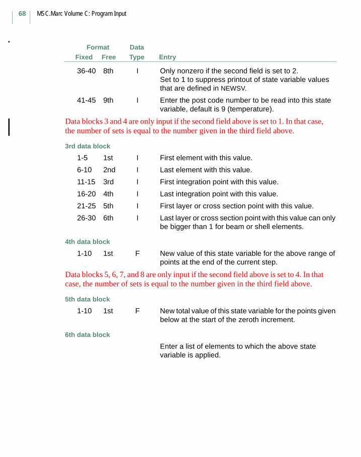
MSC.Marc Volume C: Program Input
68
FormatFree Entry
DataTypeFixed
36-40 8th I Only nonzero if the second field is set to 2. Set to 1 to suppress printout of state variable values that are defined in NEWSV.
41-45 9th I Enter the post code number to be read into this state variable, default is 9 (temperature).
Data blocks 3 and 4 are only input if the second field above is set to 1. In that case, the number of sets is equal to the number given in the third field above.
3rd data block
1-5 1st I First element with this value.
6-10 2nd I Last element with this value.
11-15 3rd I First integration point with this value.
16-20 4th I Last integration point with this value.
21-25 5th I First layer or cross section point with this value.
26-30 6th I Last layer or cross section point with this value can only be bigger than 1 for beam or shell elements.
4th data block
1-10 1st F New value of this state variable for the above range of points at the end of the current step.
Data blocks 5, 6, 7, and 8 are only input if the second field above is set to 4. In that case, the number of sets is equal to the number given in the third field above.
5th data block
1-10 1st F New total value of this state variable for the points given below at the start of the zeroth increment.
6th data block
Enter a list of elements to which the above state variable is applied.

Chapter 3 Model Definition Options69
FormatFree Entry
DataTypeFixed
7th data block
This data block is not necessary if the CENTROID parameter is used.
Enter a list of integration points to which the above state variable is applied.
8th data block
This data block is only necessary if there are either beams or shells in the mesh.
Enter a list of layer points to which the above state variable is applied.
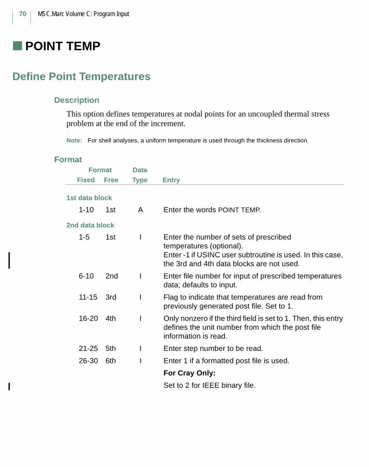
MSC.Marc Volume C: Program Input
70
POINT TEMP (Model Definition)
Define Point Temperatures
Description
This option defines temperatures at nodal points for an uncoupled thermal stress problem at the end of the increment.
Note: For shell analyses, a uniform temperature is used through the thickness direction.
FormatFree Entry
DataTypeFixed
Format
1st data block
1-10 1st A Enter the words POINT TEMP.
2nd data block
1-5 1st I Enter the number of sets of prescribed temperatures (optional).Enter -1 if USINC user subtroutine is used. In this case, the 3rd and 4th data blocks are not used.
6-10 2nd I Enter file number for input of prescribed temperatures data; defaults to input.
11-15 3rd I Flag to indicate that temperatures are read from previously generated post file. Set to 1.
16-20 4th I Only nonzero if the third field is set to 1. Then, this entry defines the unit number from which the post file information is read.
21-25 5th I Enter step number to be read.
26-30 6th I Enter 1 if a formatted post file is used.
For Cray Only:
Set to 2 for IEEE binary file.
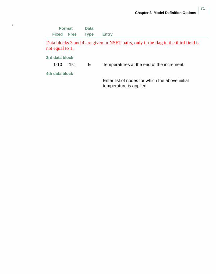
Chapter 3 Model Definition Options71
FormatFree Entry
DataTypeFixed
Data blocks 3 and 4 are given in NSET pairs, only if the flag in the third field is not equal to 1.
3rd data block
1-10 1st E Temperatures at the end of the increment.
4th data block
Enter list of nodes for which the above initial temperature is applied.
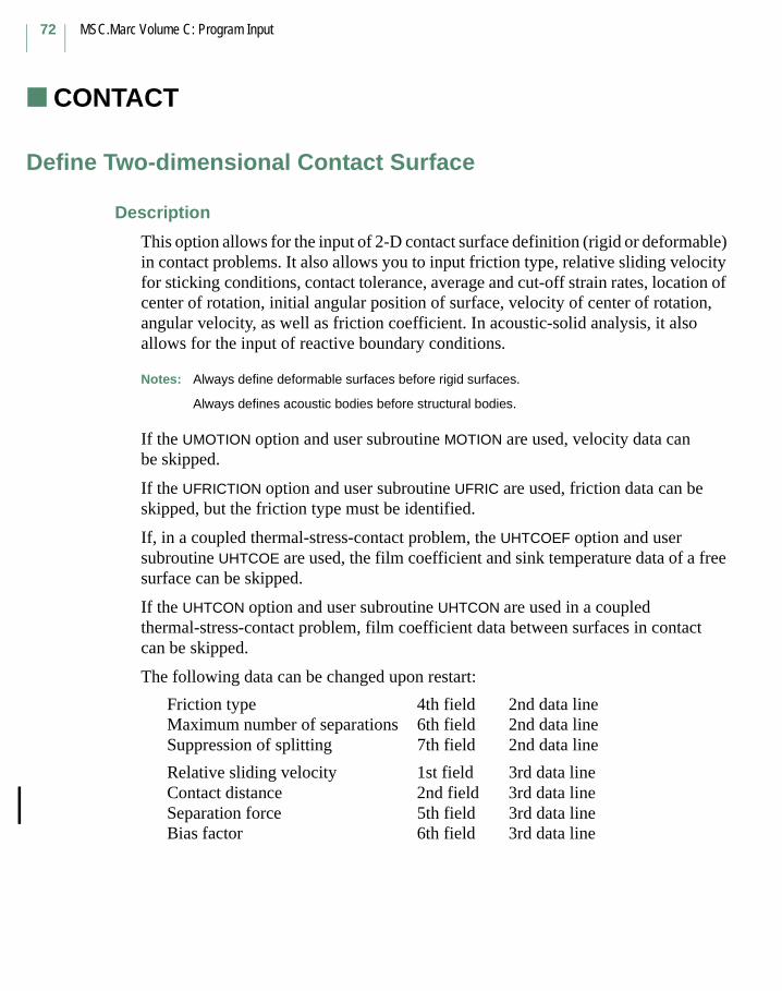
MSC.Marc Volume C: Program Input
72
CONTACT (2-D)
Define Two-dimensional Contact Surface
Description
This option allows for the input of 2-D contact surface definition (rigid or deformable) in contact problems. It also allows you to input friction type, relative sliding velocity for sticking conditions, contact tolerance, average and cut-off strain rates, location of center of rotation, initial angular position of surface, velocity of center of rotation, angular velocity, as well as friction coefficient. In acoustic-solid analysis, it also allows for the input of reactive boundary conditions.
Notes: Always define deformable surfaces before rigid surfaces.
Always defines acoustic bodies before structural bodies.
If the UMOTION option and user subroutine MOTION are used, velocity data can be skipped.
If the UFRICTION option and user subroutine UFRIC are used, friction data can be skipped, but the friction type must be identified.
If, in a coupled thermal-stress-contact problem, the UHTCOEF option and user subroutine UHTCOE are used, the film coefficient and sink temperature data of a free surface can be skipped.
If the UHTCON option and user subroutine UHTCON are used in a coupled thermal-stress-contact problem, film coefficient data between surfaces in contact can be skipped.
The following data can be changed upon restart:
Friction type 4th field 2nd data lineMaximum number of separations 6th field 2nd data lineSuppression of splitting 7th field 2nd data line
Relative sliding velocity 1st field 3rd data lineContact distance 2nd field 3rd data lineSeparation force 5th field 3rd data lineBias factor 6th field 3rd data line
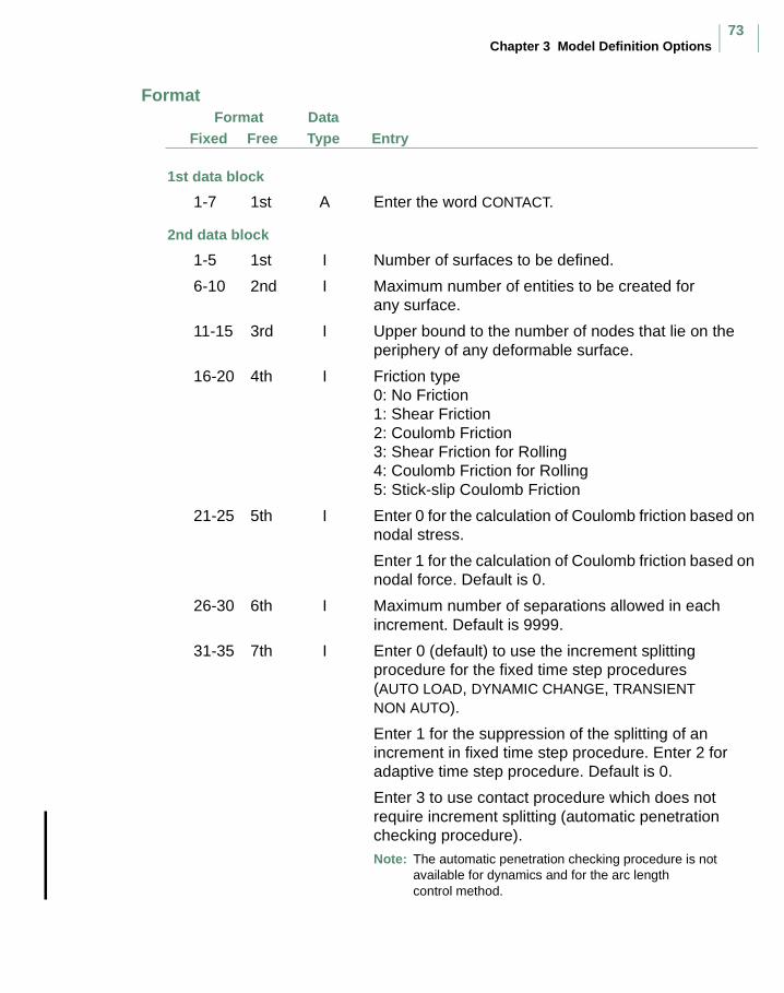
Chapter 3 Model Definition Options73
FormatFree Entry
DataTypeFixed
Format
1st data block
1-7 1st A Enter the word CONTACT.
2nd data block
1-5 1st I Number of surfaces to be defined.
6-10 2nd I Maximum number of entities to be created for any surface.
11-15 3rd I Upper bound to the number of nodes that lie on the periphery of any deformable surface.
16-20 4th I Friction type0: No Friction 1: Shear Friction 2: Coulomb Friction3: Shear Friction for Rolling4: Coulomb Friction for Rolling5: Stick-slip Coulomb Friction
21-25 5th I Enter 0 for the calculation of Coulomb friction based on nodal stress.
Enter 1 for the calculation of Coulomb friction based on nodal force. Default is 0.
26-30 6th I Maximum number of separations allowed in each increment. Default is 9999.
31-35 7th I Enter 0 (default) to use the increment splitting procedure for the fixed time step procedures (AUTO LOAD, DYNAMIC CHANGE, TRANSIENT NON AUTO).
Enter 1 for the suppression of the splitting of an increment in fixed time step procedure. Enter 2 for adaptive time step procedure. Default is 0.
Enter 3 to use contact procedure which does not require increment splitting (automatic penetration checking procedure).Note: The automatic penetration checking procedure is not
available for dynamics and for the arc length control method.
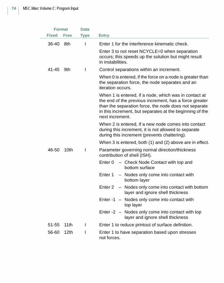
MSC.Marc Volume C: Program Input
74
FormatFree Entry
DataTypeFixed
36-40 8th I Enter 1 for the interference kinematic check.
Enter 3 to not reset NCYCLE=0 when separation occurs; this speeds up the solution but might result in instabilities.
41-45 9th I Control separations within an increment.
When 0 is entered, if the force on a node is greater than the separation force, the node separates and an iteration occurs.
When 1 is entered, if a node, which was in contact at the end of the previous increment, has a force greater than the separation force, the node does not separate in this increment, but separates at the beginning of the next increment.
When 2 is entered, if a new node comes into contact during this increment, it is not allowed to separate during this increment (prevents chattering).
When 3 is entered, both (1) and (2) above are in effect.
46-50 10th I Parameter governing normal direction/thickness contribution of shell (ISH).
Enter 0 – Check Node Contact with top and bottom surface
Enter 1 – Nodes only come into contact with bottom layer
Enter 2 – Nodes only come into contact with bottom layer and ignore shell thickness
Enter -1 – Nodes only come into contact with top layer
Enter -2 – Nodes only come into contact with top layer and ignore shell thickness
51-55 11th I Enter 1 to reduce printout of surface definition.
56-60 12th I Enter 1 to have separation based upon stresses not forces.
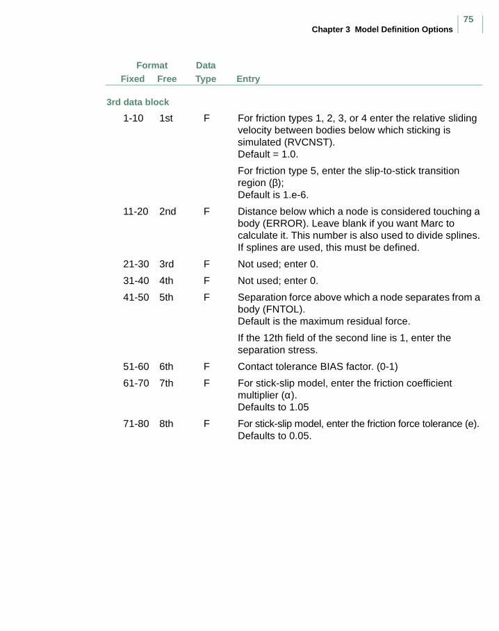
Chapter 3 Model Definition Options75
FormatFree Entry
DataTypeFixed
3rd data block
1-10 1st F For friction types 1, 2, 3, or 4 enter the relative sliding velocity between bodies below which sticking is simulated (RVCNST).Default = 1.0.
For friction type 5, enter the slip-to-stick transition region (β);Default is 1.e-6.
11-20 2nd F Distance below which a node is considered touching a body (ERROR). Leave blank if you want Marc to calculate it. This number is also used to divide splines. If splines are used, this must be defined.
21-30 3rd F Not used; enter 0.
31-40 4th F Not used; enter 0.
41-50 5th F Separation force above which a node separates from a body (FNTOL).Default is the maximum residual force.
If the 12th field of the second line is 1, enter the separation stress.
51-60 6th F Contact tolerance BIAS factor. (0-1)
61-70 7th F For stick-slip model, enter the friction coefficient multiplier (α).Defaults to 1.05
71-80 8th F For stick-slip model, enter the friction force tolerance (e).Defaults to 0.05.
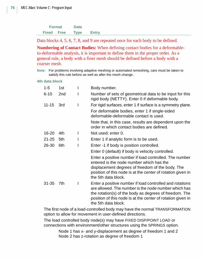
MSC.Marc Volume C: Program Input
76
FormatFree Entry
DataTypeFixed
Data blocks 4, 5, 6, 7, 8, and 9 are repeated once for each body to be defined.
Numbering of Contact Bodies: When defining contact bodies for a deformable-to-deformable analysis, it is important to define them in the proper order. As a general rule, a body with a finer mesh should be defined before a body with a coarser mesh.
Note: For problems involving adaptive meshing or automated remeshing, care must be taken to satisfy this rule before as well as after the mesh change.
4th data block
1-5 1st I Body number.
6-10 2nd I Number of sets of geometrical data to be input for this rigid body (NETTY). Enter 0 if deformable body.
11-15 3rd I For rigid surfaces, enter 1 if surface is a symmetry plane.
For deformable bodies, enter 1 if single-sided deformable-deformable contact is used.
Note that, in this case, results are dependent upon the order in which contact bodies are defined.
16-20 4th I Not used; enter 0.
21-25 5th I Enter 1 if analytic form is to be used.
26-30 6th I Enter -1 if body is position controlled.
Enter 0 (default) if body is velocity controlled.
Enter a positive number if load controlled. The number entered is the node number which has the displacement degrees of freedom of the body. The position of this node is at the center of rotation given in the 5th data block.
31-35 7th I Enter a positive number if load controlled and rotations are allowed. The number is the node number which has the rotation(s) of the body as degrees of freedom. The position of this node is at the center of rotation given in the 5th data block.
The first node of a load-controlled body may have the normal TRANSFORMATION option to allow for movement in user-defined directions.
The load controlled body node(s) may have FIXED DISP/POINT LOAD or connections with environment/other structures using the SPRINGS option.
Node 1 has x- and y-displacement as degree of freedom 1 and 2Node 2 has z-rotation as degree of freedom 1
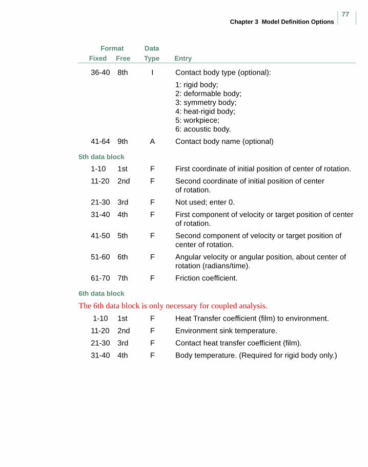
Chapter 3 Model Definition Options77
FormatFree Entry
DataTypeFixed
36-40 8th I Contact body type (optional):
1: rigid body;2: deformable body;3: symmetry body;4: heat-rigid body;5: workpiece;6: acoustic body.
41-64 9th A Contact body name (optional)
5th data block
1-10 1st F First coordinate of initial position of center of rotation.
11-20 2nd F Second coordinate of initial position of center of rotation.
21-30 3rd F Not used; enter 0.
31-40 4th F First component of velocity or target position of center of rotation.
41-50 5th F Second component of velocity or target position of center of rotation.
51-60 6th F Angular velocity or angular position, about center of rotation (radians/time).
61-70 7th F Friction coefficient.
6th data block
The 6th data block is only necessary for coupled analysis.
1-10 1st F Heat Transfer coefficient (film) to environment.
11-20 2nd F Environment sink temperature.
21-30 3rd F Contact heat transfer coefficient (film).
31-40 4th F Body temperature. (Required for rigid body only.)
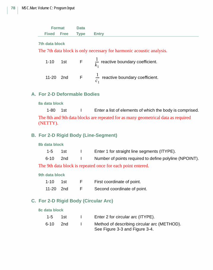
MSC.Marc Volume C: Program Input
78
FormatFree Entry
DataTypeFixed
7th data block
The 7th data block is only necessary for harmonic acoustic analysis.
1-10 1st F reactive boundary coefficient.
11-20 2nd F reactive boundary coefficient.
A. For 2-D Deformable Bodies
8a data block
1-80 1st I Enter a list of elements of which the body is comprised.
The 8th and 9th data blocks are repeated for as many geometrical data as required (NETTY).
B. For 2-D Rigid Body (Line-Segment)
8b data block
1-5 1st I Enter 1 for straight line segments (ITYPE).
6-10 2nd I Number of points required to define polyline (NPOINT).
The 9th data block is repeated once for each point entered.
9th data block
1-10 1st F First coordinate of point.
11-20 2nd F Second coordinate of point.
C. For 2-D Rigid Body (Circular Arc)
8c data block
1-5 1st I Enter 2 for circular arc (ITYPE).
6-10 2nd I Method of describing circular arc (METHOD). See Figure 3-3 and Figure 3-4.
1k1-----
1c1-----
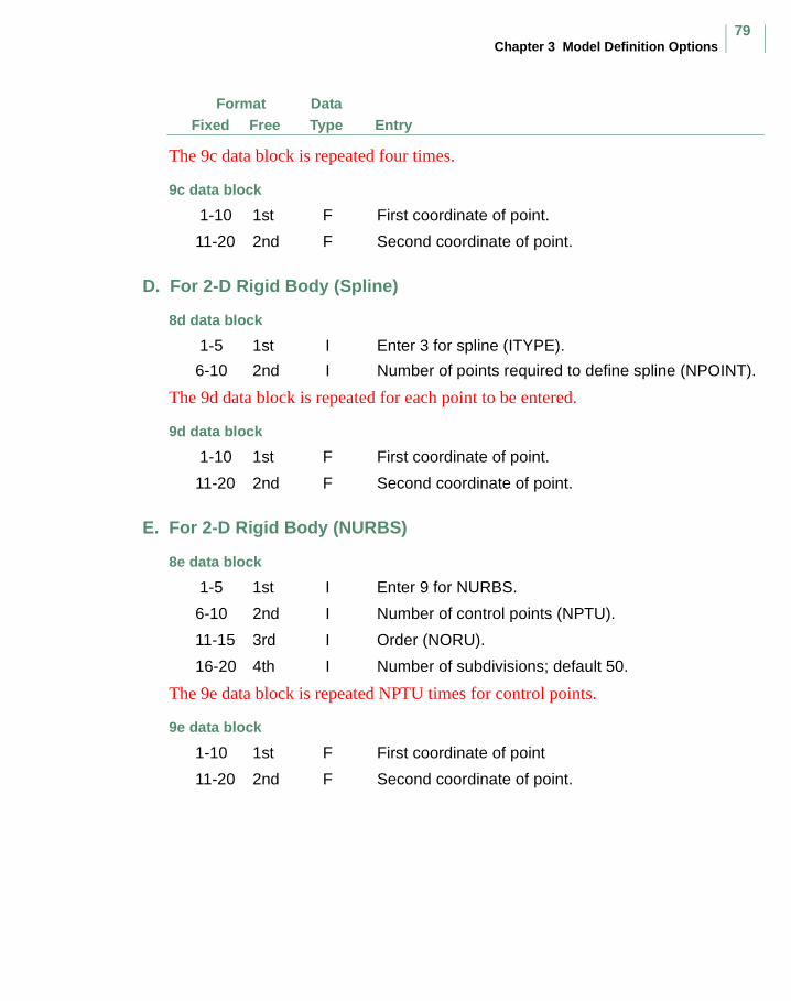
Chapter 3 Model Definition Options79
FormatFree Entry
DataTypeFixed
The 9c data block is repeated four times.
9c data block
1-10 1st F First coordinate of point.
11-20 2nd F Second coordinate of point.
D. For 2-D Rigid Body (Spline)
8d data block
1-5 1st I Enter 3 for spline (ITYPE).
6-10 2nd I Number of points required to define spline (NPOINT).
The 9d data block is repeated for each point to be entered.
9d data block
1-10 1st F First coordinate of point.
11-20 2nd F Second coordinate of point.
E. For 2-D Rigid Body (NURBS)
8e data block
1-5 1st I Enter 9 for NURBS.
6-10 2nd I Number of control points (NPTU).
11-15 3rd I Order (NORU).
16-20 4th I Number of subdivisions; default 50.
The 9e data block is repeated NPTU times for control points.
9e data block
1-10 1st F First coordinate of point
11-20 2nd F Second coordinate of point.
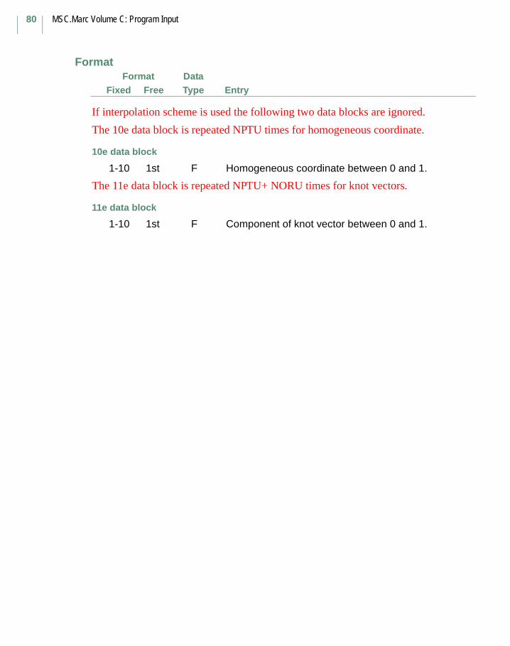
MSC.Marc Volume C: Program Input
80
FormatFree Entry
DataTypeFixed
Format
If interpolation scheme is used the following two data blocks are ignored.
The 10e data block is repeated NPTU times for homogeneous coordinate.
10e data block
1-10 1st F Homogeneous coordinate between 0 and 1.
The 11e data block is repeated NPTU+ NORU times for knot vectors.
11e data block
1-10 1st F Component of knot vector between 0 and 1.
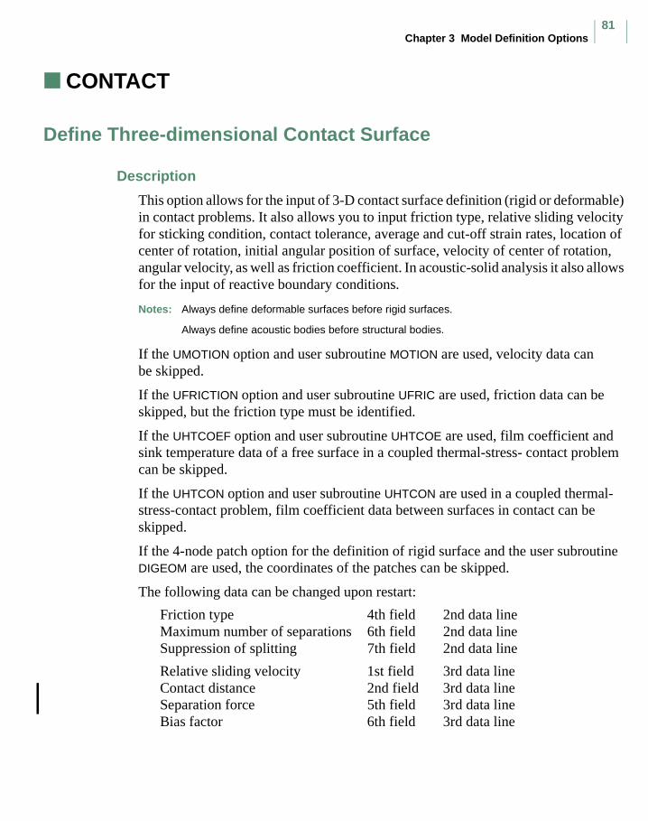
Chapter 3 Model Definition Options81
CONTACT (3-D)
Define Three-dimensional Contact Surface
Description
This option allows for the input of 3-D contact surface definition (rigid or deformable) in contact problems. It also allows you to input friction type, relative sliding velocity for sticking condition, contact tolerance, average and cut-off strain rates, location of center of rotation, initial angular position of surface, velocity of center of rotation, angular velocity, as well as friction coefficient. In acoustic-solid analysis it also allows for the input of reactive boundary conditions.
Notes: Always define deformable surfaces before rigid surfaces.
Always define acoustic bodies before structural bodies.
If the UMOTION option and user subroutine MOTION are used, velocity data can be skipped.
If the UFRICTION option and user subroutine UFRIC are used, friction data can be skipped, but the friction type must be identified.
If the UHTCOEF option and user subroutine UHTCOE are used, film coefficient and sink temperature data of a free surface in a coupled thermal-stress- contact problem can be skipped.
If the UHTCON option and user subroutine UHTCON are used in a coupled thermal-stress-contact problem, film coefficient data between surfaces in contact can be skipped.
If the 4-node patch option for the definition of rigid surface and the user subroutine DIGEOM are used, the coordinates of the patches can be skipped.
The following data can be changed upon restart:
Friction type 4th field 2nd data lineMaximum number of separations 6th field 2nd data lineSuppression of splitting 7th field 2nd data line
Relative sliding velocity 1st field 3rd data lineContact distance 2nd field 3rd data lineSeparation force 5th field 3rd data lineBias factor 6th field 3rd data line
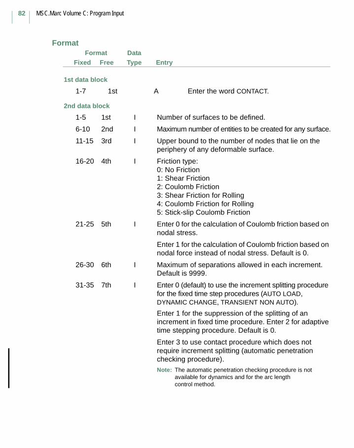
MSC.Marc Volume C: Program Input
82
FormatFree Entry
DataTypeFixed
Format
1st data block
1-7 1st A Enter the word CONTACT.
2nd data block
1-5 1st I Number of surfaces to be defined.
6-10 2nd I Maximum number of entities to be created for any surface.
11-15 3rd I Upper bound to the number of nodes that lie on the periphery of any deformable surface.
16-20 4th I Friction type:0: No Friction 1: Shear Friction2: Coulomb Friction3: Shear Friction for Rolling4: Coulomb Friction for Rolling5: Stick-slip Coulomb Friction
21-25 5th I Enter 0 for the calculation of Coulomb friction based on nodal stress.
Enter 1 for the calculation of Coulomb friction based on nodal force instead of nodal stress. Default is 0.
26-30 6th I Maximum of separations allowed in each increment. Default is 9999.
31-35 7th I Enter 0 (default) to use the increment splitting procedure for the fixed time step procedures (AUTO LOAD, DYNAMIC CHANGE, TRANSIENT NON AUTO).
Enter 1 for the suppression of the splitting of an increment in fixed time procedure. Enter 2 for adaptive time stepping procedure. Default is 0.
Enter 3 to use contact procedure which does not require increment splitting (automatic penetration checking procedure).Note: The automatic penetration checking procedure is not
available for dynamics and for the arc length control method.
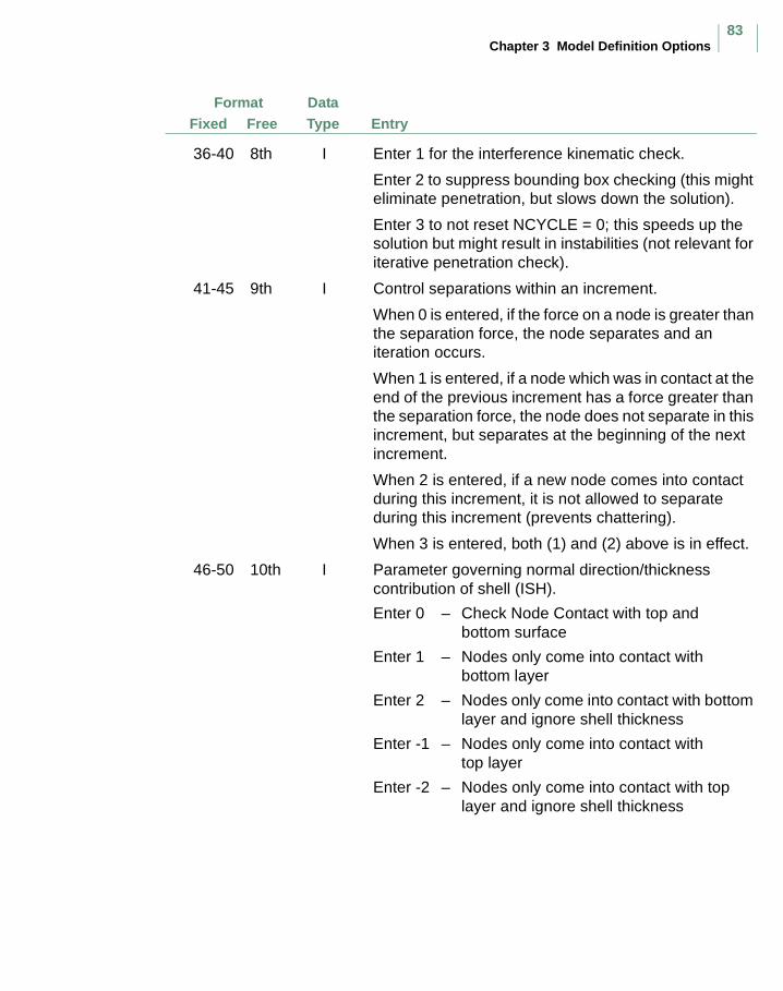
Chapter 3 Model Definition Options83
FormatFree Entry
DataTypeFixed
36-40 8th I Enter 1 for the interference kinematic check.
Enter 2 to suppress bounding box checking (this might eliminate penetration, but slows down the solution).
Enter 3 to not reset NCYCLE = 0; this speeds up the solution but might result in instabilities (not relevant for iterative penetration check).
41-45 9th I Control separations within an increment.
When 0 is entered, if the force on a node is greater than the separation force, the node separates and an iteration occurs.
When 1 is entered, if a node which was in contact at the end of the previous increment has a force greater than the separation force, the node does not separate in this increment, but separates at the beginning of the next increment.
When 2 is entered, if a new node comes into contact during this increment, it is not allowed to separate during this increment (prevents chattering).
When 3 is entered, both (1) and (2) above is in effect.
46-50 10th I Parameter governing normal direction/thickness contribution of shell (ISH).
Enter 0 – Check Node Contact with top and bottom surface
Enter 1 – Nodes only come into contact with bottom layer
Enter 2 – Nodes only come into contact with bottom layer and ignore shell thickness
Enter -1 – Nodes only come into contact with top layer
Enter -2 – Nodes only come into contact with top layer and ignore shell thickness

MSC.Marc Volume C: Program Input
84
FormatFree Entry
DataTypeFixed
51-55 11th I Enter 1 to reduce printout of surface definition.
56-60 12th I Enter 1 to have separation based upon stressesnot forces.
61-65 13th I Enter 1 to activate beam-beam contact.
3rd data block
1-10 1st F For friction types 1, 2, 3, or 4 enter the relative sliding velocity between bodies below which sticking is simulated (RVCNST).Default is 1.0.
For friction type 5, enter the slip-to-stick transition region (β);Default is 1.e-6.
11-20 2nd F Distance below which a node is considered touching a body (ERROR). Leave it blank if you want Marc to calculate it.
21-30 3rd F Not used.
31-40 4th F Not used.
41-50 5th F Separation force, above which a node separates from a body (FNTOL). Default is the maximum residual force.
If the 12th field of the second line is 1, enter the separation stress.
51-60 6th F Contact tolerance BIAS factor. (0-1)
61-70 7th F For stick-slip model, enter the friction coefficient multiplier (α).Defaults to 1.05
71-80 8th F For stick-slip model, enter the friction force tolerance (e).Defaults to 0.05.
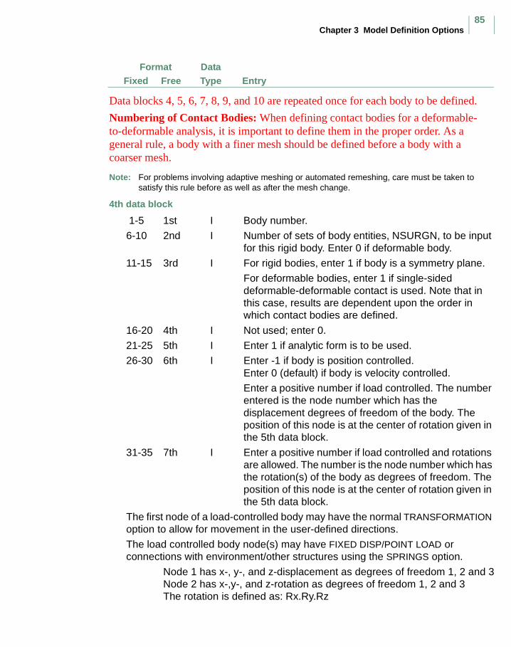
Chapter 3 Model Definition Options85
FormatFree Entry
DataTypeFixed
Data blocks 4, 5, 6, 7, 8, 9, and 10 are repeated once for each body to be defined.
Numbering of Contact Bodies: When defining contact bodies for a deformable-to-deformable analysis, it is important to define them in the proper order. As a general rule, a body with a finer mesh should be defined before a body with a coarser mesh.
Note: For problems involving adaptive meshing or automated remeshing, care must be taken to satisfy this rule before as well as after the mesh change.
4th data block
1-5 1st I Body number.
6-10 2nd I Number of sets of body entities, NSURGN, to be input for this rigid body. Enter 0 if deformable body.
11-15 3rd I For rigid bodies, enter 1 if body is a symmetry plane.
For deformable bodies, enter 1 if single-sided deformable-deformable contact is used. Note that in this case, results are dependent upon the order in which contact bodies are defined.
16-20 4th I Not used; enter 0.
21-25 5th I Enter 1 if analytic form is to be used.
26-30 6th I Enter -1 if body is position controlled.Enter 0 (default) if body is velocity controlled.
Enter a positive number if load controlled. The number entered is the node number which has the displacement degrees of freedom of the body. The position of this node is at the center of rotation given in the 5th data block.
31-35 7th I Enter a positive number if load controlled and rotations are allowed. The number is the node number which has the rotation(s) of the body as degrees of freedom. The position of this node is at the center of rotation given in the 5th data block.
The first node of a load-controlled body may have the normal TRANSFORMATION option to allow for movement in the user-defined directions.
The load controlled body node(s) may have FIXED DISP/POINT LOAD or connections with environment/other structures using the SPRINGS option.
Node 1 has x-, y-, and z-displacement as degrees of freedom 1, 2 and 3Node 2 has x-,y-, and z-rotation as degrees of freedom 1, 2 and 3The rotation is defined as: Rx.Ry.Rz
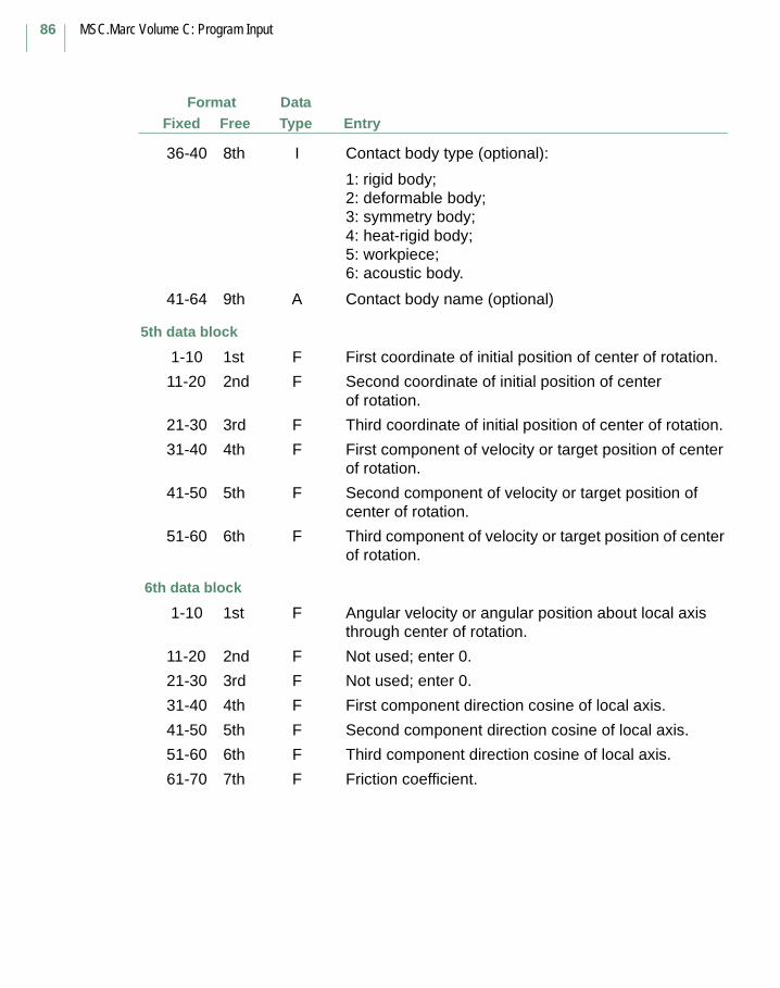
MSC.Marc Volume C: Program Input
86
FormatFree Entry
DataTypeFixed
36-40 8th I Contact body type (optional):
1: rigid body;2: deformable body;3: symmetry body;4: heat-rigid body;5: workpiece;6: acoustic body.
41-64 9th A Contact body name (optional)
5th data block
1-10 1st F First coordinate of initial position of center of rotation.
11-20 2nd F Second coordinate of initial position of center of rotation.
21-30 3rd F Third coordinate of initial position of center of rotation.
31-40 4th F First component of velocity or target position of center of rotation.
41-50 5th F Second component of velocity or target position of center of rotation.
51-60 6th F Third component of velocity or target position of center of rotation.
6th data block
1-10 1st F Angular velocity or angular position about local axis through center of rotation.
11-20 2nd F Not used; enter 0.
21-30 3rd F Not used; enter 0.
31-40 4th F First component direction cosine of local axis.
41-50 5th F Second component direction cosine of local axis.
51-60 6th F Third component direction cosine of local axis.
61-70 7th F Friction coefficient.
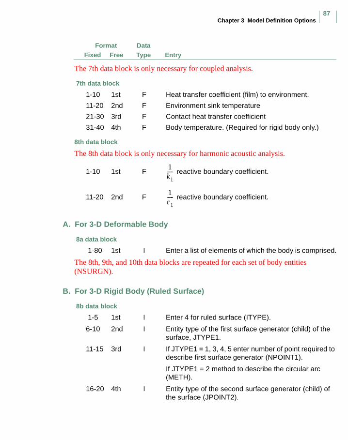
Chapter 3 Model Definition Options87
FormatFree Entry
DataTypeFixed
The 7th data block is only necessary for coupled analysis.
7th data block
1-10 1st F Heat transfer coefficient (film) to environment.
11-20 2nd F Environment sink temperature
21-30 3rd F Contact heat transfer coefficient
31-40 4th F Body temperature. (Required for rigid body only.)
8th data block
The 8th data block is only necessary for harmonic acoustic analysis.
1-10 1st F reactive boundary coefficient.
11-20 2nd F reactive boundary coefficient.
A. For 3-D Deformable Body
8a data block
1-80 1st I Enter a list of elements of which the body is comprised.
The 8th, 9th, and 10th data blocks are repeated for each set of body entities (NSURGN).
B. For 3-D Rigid Body (Ruled Surface)
8b data block
1-5 1st I Enter 4 for ruled surface (ITYPE).
6-10 2nd I Entity type of the first surface generator (child) of the surface, JTYPE1.
11-15 3rd I If JTYPE1 = 1, 3, 4, 5 enter number of point required to describe first surface generator (NPOINT1).
If JTYPE1 = 2 method to describe the circular arc (METH).
16-20 4th I Entity type of the second surface generator (child) of the surface (JPOINT2).
1k1-----
1c1-----
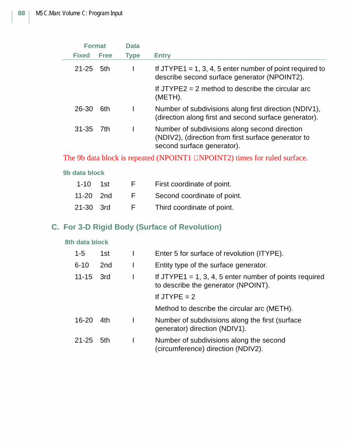
MSC.Marc Volume C: Program Input
88
FormatFree Entry
DataTypeFixed
21-25 5th I If JTYPE1 = 1, 3, 4, 5 enter number of point required to describe second surface generator (NPOINT2).
If JTYPE2 = 2 method to describe the circular arc (METH).
26-30 6th I Number of subdivisions along first direction (NDIV1), (direction along first and second surface generator).
31-35 7th I Number of subdivisions along second direction (NDIV2), (direction from first surface generator to second surface generator).
The 9b data block is repeated (NPOINT1 ∗ NPOINT2) times for ruled surface.
9b data block
1-10 1st F First coordinate of point.
11-20 2nd F Second coordinate of point.
21-30 3rd F Third coordinate of point.
C. For 3-D Rigid Body (Surface of Revolution)
8th data block
1-5 1st I Enter 5 for surface of revolution (ITYPE).
6-10 2nd I Entity type of the surface generator.
11-15 3rd I If JTYPE1 = 1, 3, 4, 5 enter number of points required to describe the generator (NPOINT).
If JTYPE = 2
Method to describe the circular arc (METH).
16-20 4th I Number of subdivisions along the first (surface generator) direction (NDIV1).
21-25 5th I Number of subdivisions along the second (circumference) direction (NDIV2).
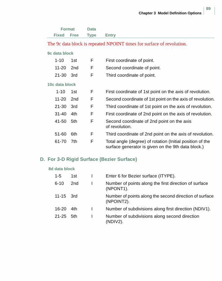
Chapter 3 Model Definition Options89
FormatFree Entry
DataTypeFixed
The 9c data block is repeated NPOINT times for surface of revolution.
9c data block
1-10 1st F First coordinate of point.
11-20 2nd F Second coordinate of point.
21-30 3rd F Third coordinate of point.
10c data block
1-10 1st F First coordinate of 1st point on the axis of revolution.
11-20 2nd F Second coordinate of 1st point on the axis of revolution.
21-30 3rd F Third coordinate of 1st point on the axis of revolution.
31-40 4th F First coordinate of 2nd point on the axis of revolution.
41-50 5th F Second coordinate of 2nd point on the axis of revolution.
51-60 6th F Third coordinate of 2nd point on the axis of revolution.
61-70 7th F Total angle (degree) of rotation (Initial position of the surface generator is given on the 9th data block.)
D. For 3-D Rigid Surface (Bezier Surface)
8d data block
1-5 1st I Enter 6 for Bezier surface (ITYPE).
6-10 2nd I Number of points along the first direction of surface (NPONT1).
11-15 3rd Number of points along the second direction of surface (NPOINT2).
16-20 4th I Number of subdivisions along first direction (NDIV1).
21-25 5th I Number of subdivisions along second direction (NDIV2).
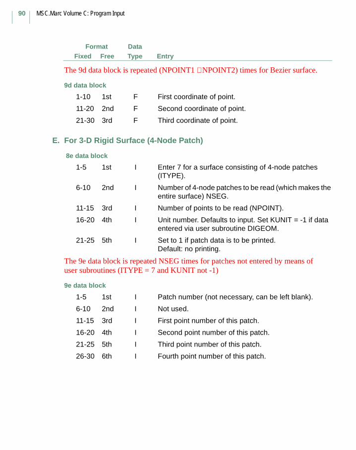
MSC.Marc Volume C: Program Input
90
FormatFree Entry
DataTypeFixed
The 9d data block is repeated (NPOINT1 ∗ NPOINT2) times for Bezier surface.
9d data block
1-10 1st F First coordinate of point.
11-20 2nd F Second coordinate of point.
21-30 3rd F Third coordinate of point.
E. For 3-D Rigid Surface (4-Node Patch)
8e data block
1-5 1st I Enter 7 for a surface consisting of 4-node patches (ITYPE).
6-10 2nd I Number of 4-node patches to be read (which makes the entire surface) NSEG.
11-15 3rd I Number of points to be read (NPOINT).
16-20 4th I Unit number. Defaults to input. Set KUNIT = -1 if data entered via user subroutine DIGEOM.
21-25 5th I Set to 1 if patch data is to be printed. Default: no printing.
The 9e data block is repeated NSEG times for patches not entered by means of user subroutines (ITYPE = 7 and KUNIT not -1)
9e data block
1-5 1st I Patch number (not necessary, can be left blank).
6-10 2nd I Not used.
11-15 3rd I First point number of this patch.
16-20 4th I Second point number of this patch.
21-25 5th I Third point number of this patch.
26-30 6th I Fourth point number of this patch.
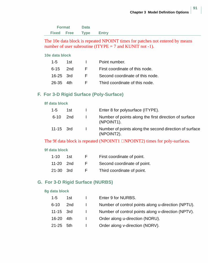
Chapter 3 Model Definition Options91
FormatFree Entry
DataTypeFixed
The 10e data block is repeated NPOINT times for patches not entered by means number of user subroutine (ITYPE = 7 and KUNIT not -1).
10e data block
1-5 1st I Point number.
6-15 2nd F First coordinate of this node.
16-25 3rd F Second coordinate of this node.
26-35 4th F Third coordinate of this node.
F. For 3-D Rigid Surface (Poly-Surface)
8f data block
1-5 1st I Enter 8 for polysurface (ITYPE).
6-10 2nd I Number of points along the first direction of surface (NPOINT1).
11-15 3rd I Number of points along the second direction of surface (NPOINT2).
The 9f data block is repeated (NPOINT1 ∗ NPOINT2) times for poly-surfaces.
9f data block
1-10 1st F First coordinate of point.
11-20 2nd F Second coordinate of point.
21-30 3rd F Third coordinate of point.
G. For 3-D Rigid Surface (NURBS)
8g data block
1-5 1st I Enter 9 for NURBS.
6-10 2nd I Number of control points along u-direction (NPTU).
11-15 3rd I Number of control points along v-direction (NPTV).
16-20 4th I Order along u-direction (NORU).
21-25 5th I Order along v-direction (NORV).
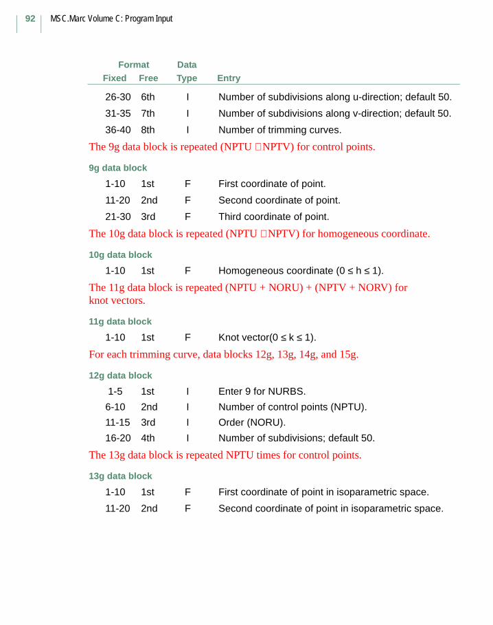
MSC.Marc Volume C: Program Input
92
FormatFree Entry
DataTypeFixed
26-30 6th I Number of subdivisions along u-direction; default 50.
31-35 7th I Number of subdivisions along v-direction; default 50.
36-40 8th I Number of trimming curves.
The 9g data block is repeated (NPTU ∗ NPTV) for control points.
9g data block
1-10 1st F First coordinate of point.
11-20 2nd F Second coordinate of point.
21-30 3rd F Third coordinate of point.
The 10g data block is repeated (NPTU ∗ NPTV) for homogeneous coordinate.
10g data block
1-10 1st F Homogeneous coordinate (0 ≤ h ≤ 1).
The 11g data block is repeated (NPTU + NORU) + (NPTV + NORV) for knot vectors.
11g data block
1-10 1st F Knot vector(0 ≤ k ≤ 1).
For each trimming curve, data blocks 12g, 13g, 14g, and 15g.
12g data block
1-5 1st I Enter 9 for NURBS.
6-10 2nd I Number of control points (NPTU).
11-15 3rd I Order (NORU).
16-20 4th I Number of subdivisions; default 50.
The 13g data block is repeated NPTU times for control points.
13g data block
1-10 1st F First coordinate of point in isoparametric space.
11-20 2nd F Second coordinate of point in isoparametric space.
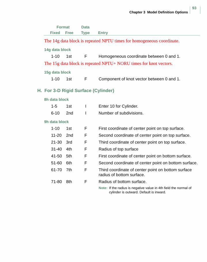
Chapter 3 Model Definition Options93
FormatFree Entry
DataTypeFixed
The 14g data block is repeated NPTU times for homogeneous coordinate.
14g data block
1-10 1st F Homogeneous coordinate between 0 and 1.
The 15g data block is repeated NPTU+ NORU times for knot vectors.
15g data block
1-10 1st F Component of knot vector between 0 and 1.
H. For 3-D Rigid Surface (Cylinder)
8h data block
1-5 1st I Enter 10 for Cylinder.
6-10 2nd I Number of subdivisions.
9h data block
1-10 1st F First coordinate of center point on top surface.
11-20 2nd F Second coordinate of center point on top surface.
21-30 3rd F Third coordinate of center point on top surface.
31-40 4th F Radius of top surface
41-50 5th F First coordinate of center point on bottom surface.
51-60 6th F Second coordinate of center point on bottom surface.
61-70 7th F Third coordinate of center point on bottom surface radius of bottom surface.
71-80 8th F Radius of bottom surface.Note: If the radius is negative value in 4th field the normal of
cylinder is outward. Default is inward.

MSC.Marc Volume C: Program Input
94
FormatFree Entry
DataTypeFixed
I. For 3-D Rigid Surface (Sphere)
8i data block
1-5 1st I Enter 11 for Sphere.
6-10 2nd I Number of subdivisions.
9i data block
1-10 1st F First coordinate of center point.
11-20 2nd F Second coordinate of center point.
21-30 3rd F Third coordinate of center point.
31-40 4th F Radius of sphere.Note: If the radius is negative value in 4th field, the normal of
sphere is outward. Default is inward.
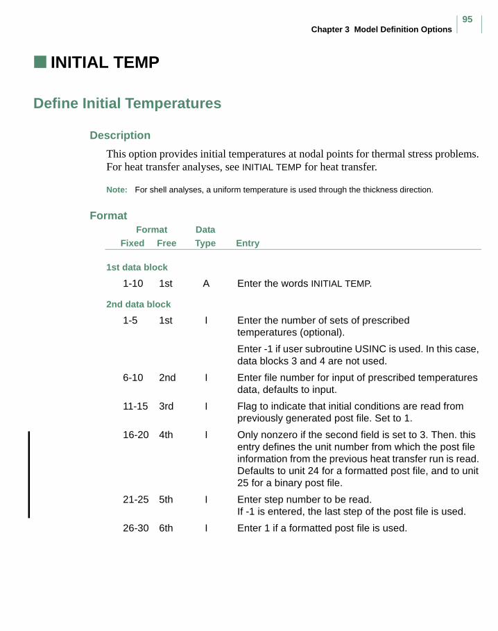
Chapter 3 Model Definition Options95
INITIAL TEMP (Thermal Stress)
Define Initial Temperatures
Description
This option provides initial temperatures at nodal points for thermal stress problems. For heat transfer analyses, see INITIAL TEMP for heat transfer.
Note: For shell analyses, a uniform temperature is used through the thickness direction.
FormatFree Entry
DataTypeFixed
Format
1st data block
1-10 1st A Enter the words INITIAL TEMP.
2nd data block
1-5 1st I Enter the number of sets of prescribed temperatures (optional).
Enter -1 if user subroutine USINC is used. In this case, data blocks 3 and 4 are not used.
6-10 2nd I Enter file number for input of prescribed temperatures data, defaults to input.
11-15 3rd I Flag to indicate that initial conditions are read from previously generated post file. Set to 1.
16-20 4th I Only nonzero if the second field is set to 3. Then. this entry defines the unit number from which the post file information from the previous heat transfer run is read. Defaults to unit 24 for a formatted post file, and to unit 25 for a binary post file.
21-25 5th I Enter step number to be read.If -1 is entered, the last step of the post file is used.
26-30 6th I Enter 1 if a formatted post file is used.

MSC.Marc Volume C: Program Input
96
FormatFree Entry
DataTypeFixed
Data blocks 3 and 4 are given in NSET pairs, only if the flag in the third field is not equal to 1.
3rd data block
1-10 1st E Initial temperature.
4th data block
Enter list of nodes for which the above initial temperature is applied.
Chapter 3 Model Definition Options97
CONTACT TABLE (Model Definition)
Define Contact Table
Description
This option is useful for deactivating or activating bodies when the CONTACT option is used. To avoid unnecessary detection of contact between bodies, you can control the detection of contact. The default for contact analysis is that every body detects the possibility of contact relative to all other bodies and itself if it is a flexible body. When the CONTACT TABLE option is entered, the default of detection for every body is overridden. Instead, you specify the relationship of detection between bodies for contact. The touching body does not contact itself unless you request it. Whenever the touched body is a flexible one, by default, the capability of double-sided contact is applied between the contacting bodies. This can be switched off by selecting single-sided contact on the CONTACT option or by setting the searching order in the CONTACT TABLE option. A positive value of the interference closure implies that there is an overlap between the bodies; a negative value implies that a gap exists.
The following control variables of contact between bodies can be modified throughout the table: contact tolerance, separation force, friction coefficient, interference closure and contact heat transfer coefficient (for coupled thermal-stress-contact analysis). In addition, you can invoke the glue option. The previous values of those control variables is not overridden unless nonzero values are entered here. For an acoustic-solid analysis, you can also modify the reactive boundary coefficients.
In the glue option, when a node contacts a rigid body, the relative tangential displacement is zero. When a node contacts a deformable body, all the translational degrees of freedom are tied.
Notes: This option should be placed after the CONTACT option.
In a restart analysis, if these values are to be changed, use the REAUTO option and specify the CONTACT TABLE after the END OPTION.

MSC.Marc Volume C: Program Input
98
FormatFree Entry
DataTypeFixed
Format
1st data block
1-10 1st A Enter the word CONTACT TABLE.
2nd data block
1-5 1st I Enter the number of sets of bodies to be input.
The 3rd, 4th, and 5th data blocks are entered once for each set of bodies to be input.
3rd data block
1-5 1st I Enter the touching body number.
6-15 2nd F Enter the contact tolerance (ERROR).
16-25 3rd F Enter the contact separation force (FNTOL).
26-35 4th F Enter the friction coefficient.
36-45 5th F Enter the interference closure amount, normal to the contact surface.
46-55 6th F Enter the contact heat transfer coefficient (coupled analysis only).
56-65 7th F Enter 1.0 to invoke the condition that, when a node comes into contact with this body, there is no relative normal or tangential displacement.
Enter 2.0 to invoke the condition that a node is initially in contact with this body (there can be a small gap or overclosure) and there is no relative normal or tangential displacement. The node is not projected onto the surface.

Chapter 3 Model Definition Options99
FormatFree Entry
DataTypeFixed
66-70 8th I Enter 1 to indicate that the searching order for deformable contact bodies is from the touching body to the touched bodies on the 5th data block. This might change the default order for deformable bodies, which is from bodies with a lower number to bodies with a higher number.
Enter 2 to let the program decide which searching order is optimal for deformable bodies. This order is set up such that searching is done starting with the body having the smallest element edge. This option forces single-sided contact between the touching and touched bodies: searching is done only from one body to another and not the other way around.
71-75 9th I Enter 1 to modify the coordinates of a node in contact with a deformable body so that stress-free initial contact can be obtained.
Enter 2 to extend the tangential error tolerance at sharp corners of deformable bodies to delay sliding off a contacted segment.
Enter 3 to have both 1 and 2 active.
4th data block (Only necessary for harmonic acoustic analysis)
1-10 1st F Enter the reactive boundary coefficient.
11-20 2nd F Enter the reactive boundary coefficient.
5th data block
Enter a list of bodies for which the touching body detects contact with the parameters above.
1k1-----
1c1-----
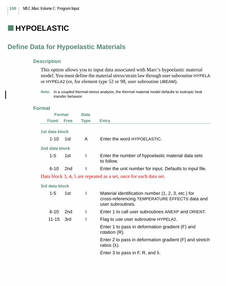
MSC.Marc Volume C: Program Input
100
HYPOELASTIC
Define Data for Hypoelastic Materials
Description
This option allows you to input data associated with Marc’s hypoelastic material model. You must define the material stress/strain law through user subroutine HYPELA or HYPELA2 (or, for element type 52 or 98, user subroutine UBEAM).
Note: In a coupled thermal-stress analysis, the thermal material model defaults to isotropic heat transfer behavior.
FormatFree Entry
DataTypeFixed
Format
1st data block
1-10 1st A Enter the word HYPOELASTIC.
2nd data block
1-5 1st I Enter the number of hypoelastic material data sets to follow.
6-10 2nd I Enter the unit number for input. Defaults to input file.
Data block 3, 4, 5 are repeated as a set, once for each data set.
3rd data block
1-5 1st I Material identification number (1, 2, 3, etc.) for cross-referencing TEMPERATURE EFFECTS data and user subroutines.
6-10 2nd I Enter 1 to call user subroutines ANEXP and ORIENT.
11-15 3rd I Flag to use user subroutine HYPELA2.
Enter 1 to pass in deformation gradient (F) and rotation (R).
Enter 2 to pass in deformation gradient (F) and stretch ratios (λ).
Enter 3 to pass in F, R, and λ.
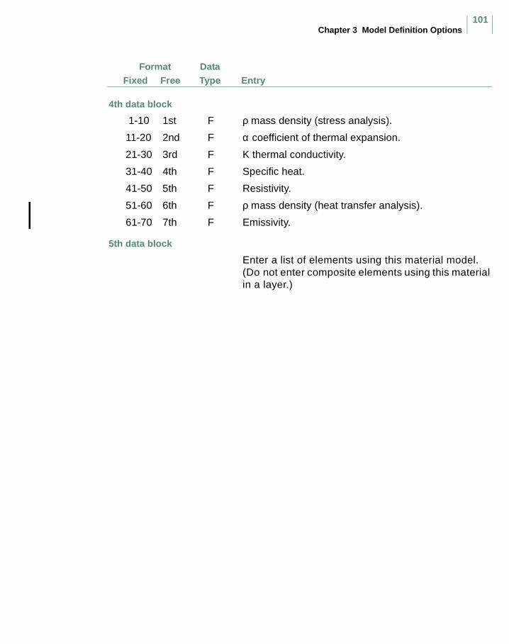
Chapter 3 Model Definition Options101
FormatFree Entry
DataTypeFixed
4th data block
1-10 1st F ρ mass density (stress analysis).
11-20 2nd F α coefficient of thermal expansion.
21-30 3rd F K thermal conductivity.
31-40 4th F Specific heat.
41-50 5th F Resistivity.
51-60 6th F ρ mass density (heat transfer analysis).
61-70 7th F Emissivity.
5th data block
Enter a list of elements using this material model. (Do not enter composite elements using this material in a layer.)

MSC.Marc Volume C: Program Input
102
MOONEY
Define Data for Mooney-Rivlin Materials
Description
This option allows you to enter all the material data for a Mooney-Rivlin rubber material. User subroutine UMOONY can be used to enter temperature dependent coefficients. User subroutine UENERG can be used to enter a general strain energy function. If rate effects are also present, the VISCELMOON model definition option can also be required. A list of elements can also be associated with this material.
Notes: For a Neo-Hookean material model, only C10 is needed.
For a Mooney/Rivlin material model, only C10 and C01 are needed.
For the full 3rd-order invariant model of Jamus, Green and Simpson, use all C10, C01, C11,
C20, C30.
The procedure used for the Mooney formulation is defined on the ELASTICITY parameter. If the Total Lagrange formulation is invoked, the elements in this case must be of the Herrmann formulation except for plane stress. If the Updated Lagrange formulation is invoked, the elements must be conventional displacement formulation. (Near-incompressibility is imposed using mixed approach and condensing out pressure degrees of freedom.) For plane stress, displacement elements are always used.
In a coupled thermal-stress analysis, the thermal material model defaults to isotropic heat transfer behavior
These material identifications cannot be referenced by any composite group.
The values C10, C01, C11, C20, and C30 can be redefined using the user subroutine UMOONY.
Although a general strain energy function can be defined by using the user subroutine UENERG, it is still required to define the elements associated with the material identifier here.
FormatFree Entry
DataTypeFixed
Format
1st data block
1-10 1st A Enter the word MOONEY.
2nd data block
1-5 1st I Enter the number of data sets to follow.
6-10 2nd I Unit number for data input. Defaults to input file.

Chapter 3 Model Definition Options103
FormatFree Entry
DataTypeFixed
Data blocks 3, 4, and 5 are repeated as a set, once for each data set.
3rd data block
1-5 1st I Material identification number.
4th data block
1-10 1st F C10 – Mooney-Rivlin constant.
11-20 2nd F C01 – Mooney-Rivlin constant.
21-30 3rd F ρ – mass density (stress analysis).
31-40 4th F α – coefficient of thermal expansion.
41-50 5th F C11 – higher order constants
51-60 6th F C20 – higher order constants.
61-70 7th F C30 – higher order constants.
71-80 8th F K – bulk modulus.
5th data block
Only necessary in a coupled thermal-stress analysis
1-10 1st F Conductivity.
11-20 2nd F Specific heat.
21-30 3rd F Mass density (heat transfer analysis).
31-40 4th F Electrical resistance.
41-50 5th F Emissivity.
6th data block
Enter a list of element numbers associated with this particular elastomeric material.
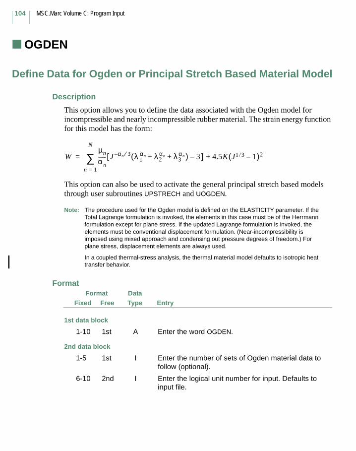
MSC.Marc Volume C: Program Input
104
OGDEN
Define Data for Ogden or Principal Stretch Based Material Model
Description
This option allows you to define the data associated with the Ogden model for incompressible and nearly incompressible rubber material. The strain energy function for this model has the form:
This option can also be used to activate the general principal stretch based models through user subroutines UPSTRECH and UOGDEN.
Note: The procedure used for the Ogden model is defined on the ELASTICITY parameter. If the Total Lagrange formulation is invoked, the elements in this case must be of the Herrmann formulation except for plane stress. If the updated Lagrange formulation is invoked, the elements must be conventional displacement formulation. (Near-incompressibility is imposed using mixed approach and condensing out pressure degrees of freedom.) For plane stress, displacement elements are always used.
In a coupled thermal-stress analysis, the thermal material model defaults to isotropic heat transfer behavior.
FormatFree Entry
DataTypeFixed
Format
1st data block
1-10 1st A Enter the word OGDEN.
2nd data block
1-5 1st I Enter the number of sets of Ogden material data to follow (optional).
6-10 2nd I Enter the logical unit number for input. Defaults to input file.
Wµn
αn------ J[ αn 3⁄– λ( 1
αn λ2αn λ3
αn ) 3–+ + ] 4.5K J1 3/ 1–( )2+
n 1=
N
∑=
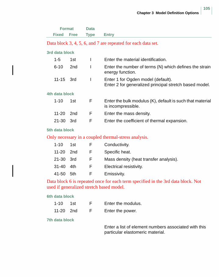
Chapter 3 Model Definition Options105
FormatFree Entry
DataTypeFixed
Data block 3, 4, 5, 6, and 7 are repeated for each data set.
3rd data block
1-5 1st I Enter the material identification.
6-10 2nd I Enter the number of terms (N) which defines the strain energy function.
11-15 3rd I Enter 1 for Ogden model (default).Enter 2 for generalized principal stretch based model.
4th data block
1-10 1st F Enter the bulk modulus (K), default is such that material is incompressible.
11-20 2nd F Enter the mass density.
21-30 3rd F Enter the coefficient of thermal expansion.
5th data block
Only necessary in a coupled thermal-stress analysis.
1-10 1st F Conductivity.
11-20 2nd F Specific heat.
21-30 3rd F Mass density (heat transfer analysis).
31-40 4th F Electrical resistivity.
41-50 5th F Emissivity.
Data block 6 is repeated once for each term specified in the 3rd data block. Not used if generalized stretch based model.
6th data block
1-10 1st F Enter the modulus.
11-20 2nd F Enter the power.
7th data block
Enter a list of element numbers associated with this particular elastomeric material.
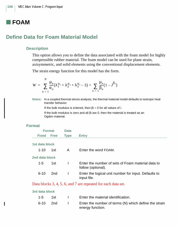
MSC.Marc Volume C: Program Input
106
FOAM
Define Data for Foam Material Model
Description
This option allows you to define the data associated with the foam model for highly compressible rubber material. The foam model can be used for plane strain, axisymmetric, and solid elements using the conventional displacement elements.
The strain energy function for this model has the form.
Notes: In a coupled thermal-stress analysis, the thermal material model defaults to isotropic heat transfer behavior.
If the bulk modulus is entered, then βi = 0 for all values of i.
If the bulk modulus is zero and all βi are 0, then the material is treated as an Ogden material.
FormatFree Entry
DataTypeFixed
Format
1st data block
1-10 1st A Enter the word FOAM.
2nd data block
1-5 1st I Enter the number of sets of Foam material data to follow (optional).
6-10 2nd I Enter the logical unit number for input. Defaults to input file.
Data blocks 3, 4, 5, 6, and 7 are repeated for each data set.
3rd data block
1-5 1st I Enter the material identification.
6-10 2nd I Enter the number of terms (N) which define the strain energy function.
Wµn
αn------ λ1
αn λ2αn λ3
αn 3–+ +( )µn
βn----- 1 J
βn–( )n 1=∑+
n 1=
N
∑=
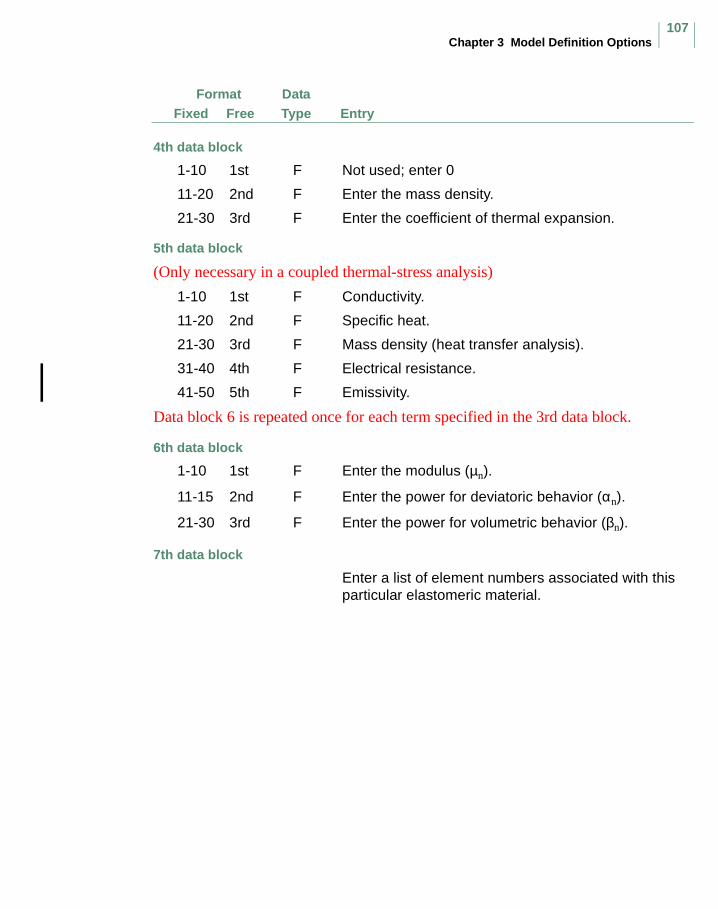
Chapter 3 Model Definition Options107
FormatFree Entry
DataTypeFixed
4th data block
1-10 1st F Not used; enter 0
11-20 2nd F Enter the mass density.
21-30 3rd F Enter the coefficient of thermal expansion.
5th data block
(Only necessary in a coupled thermal-stress analysis)
1-10 1st F Conductivity.
11-20 2nd F Specific heat.
21-30 3rd F Mass density (heat transfer analysis).
31-40 4th F Electrical resistance.
41-50 5th F Emissivity.
Data block 6 is repeated once for each term specified in the 3rd data block.
6th data block
1-10 1st F Enter the modulus (µn).
11-15 2nd F Enter the power for deviatoric behavior (αn).
21-30 3rd F Enter the power for volumetric behavior (βn).
7th data block
Enter a list of element numbers associated with this particular elastomeric material.

MSC.Marc Volume C: Program Input
108
GASKET
Define Material Data for Gasket Materials
Description
This option allows you to specify the material properties for a gasket material, such as the loading and unloading paths, the yield pressure, the transverse shear modulus, and the membrane behavior of the gasket (see also MSC.Marc Volume A: Theory and User Information). The loading and unloading paths should be defined using the TABLE option and must be given as a relation between the pressure on the gasket and the gasket closure (independent variable type 37). The reference value of these tables is always 1.
The membrane behavior should be specified using the ISOTROPIC option.
Note: This option can be used only with the lower-order solid composite element types 149, 151 and 152.
FormatFree Entry
DataTypeFixed
Format
1st data block
1-10 1st A Enter the word GASKET.
2nd data block
1-5 1st I Enter the number of sets of gasket material data to follow (optional).
6-10 2nd I Enter the unit number for input. Defaults to input file.
Data blocks 3 through 7 are repeated as a set, once for each set of gasket material to be input.
3rd data block
1-5 1st I Enter the gasket material identification number.
6-10 2nd I Enter the material identification number of the isotropic material to be used for the membrane behavior of the gasket.

Chapter 3 Model Definition Options109
FormatFree Entry
DataTypeFixed
4th data block
1-5 1st I Enter gasket behavior type in the thickness direction. Currently only type 0 (elastic-plastic) is supported.
6-10 2nd I Enter the table identification number of the loading path of the gasket.
11-15 3rd I Enter the number of unloading paths to be read through data block 4a.If a 0 is entered here, the gasket behavior will be fully elastic. Up to 10 unloading paths may be specified.
4a data block
Necessary only if the number of unloading paths entered in the 3rd field of the 4th data block is nonzero.
1-5 1st I Enter the table identification number of the first unloading path of the gasket.
6-10 2nd I Enter the table identification number of the second unloading path of the gasket if present.
11-15 3rd I Enter the table identification number of the third unloading path of the gasket if present.
16-20 4th I Enter the table identification number of the fourth unloading path of the gasket if present.
21-25 5th I Enter the table identification number of the fifth unloading path of the gasket if present.
26-30 6th I Enter the table identification number of the sixth unloading path of the gasket if present.
31-35 7th I Enter the table identification number of the seventh unloading path of the gasket if present.
36-40 8th I Enter the table identification number of the eighth unloading path of the gasket if present.
41-45 9th I Enter the table identification number of the ninth unloading path of the gasket if present.
46-50 10th I Enter the table identification number of the tenth unloading path of the gasket if present.
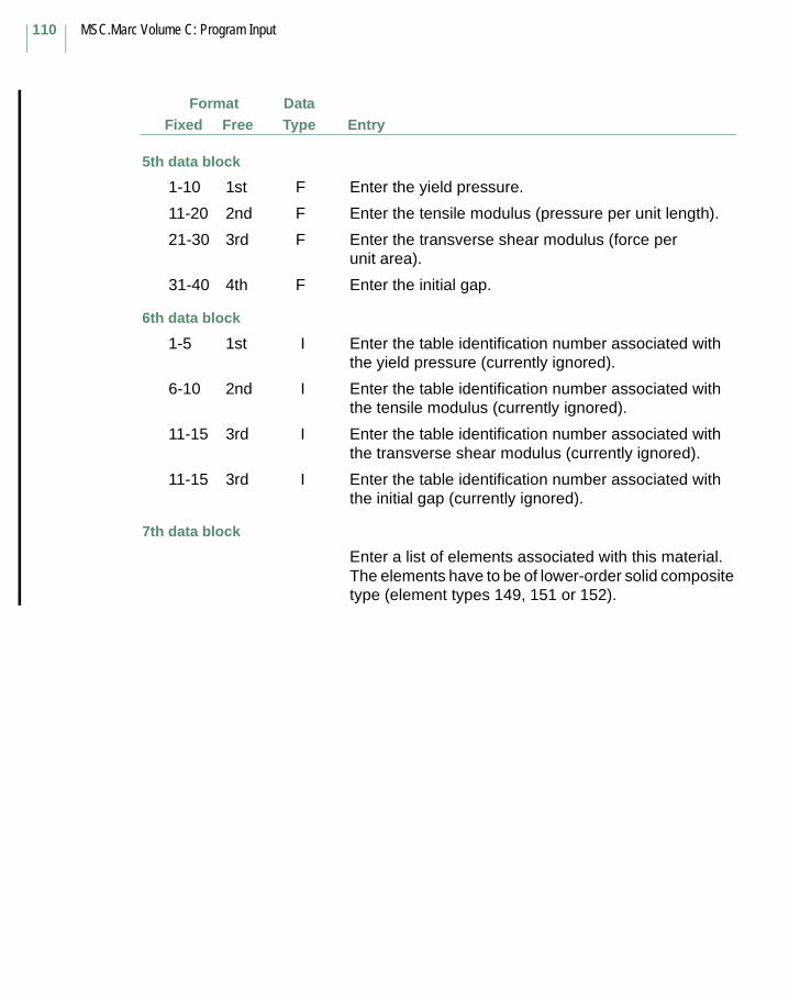
MSC.Marc Volume C: Program Input
110
FormatFree Entry
DataTypeFixed
5th data block
1-10 1st F Enter the yield pressure.
11-20 2nd F Enter the tensile modulus (pressure per unit length).
21-30 3rd F Enter the transverse shear modulus (force per unit area).
31-40 4th F Enter the initial gap.
6th data block
1-5 1st I Enter the table identification number associated with the yield pressure (currently ignored).
6-10 2nd I Enter the table identification number associated with the tensile modulus (currently ignored).
11-15 3rd I Enter the table identification number associated with the transverse shear modulus (currently ignored).
11-15 3rd I Enter the table identification number associated with the initial gap (currently ignored).
7th data block
Enter a list of elements associated with this material. The elements have to be of lower-order solid composite type (element types 149, 151 or 152).
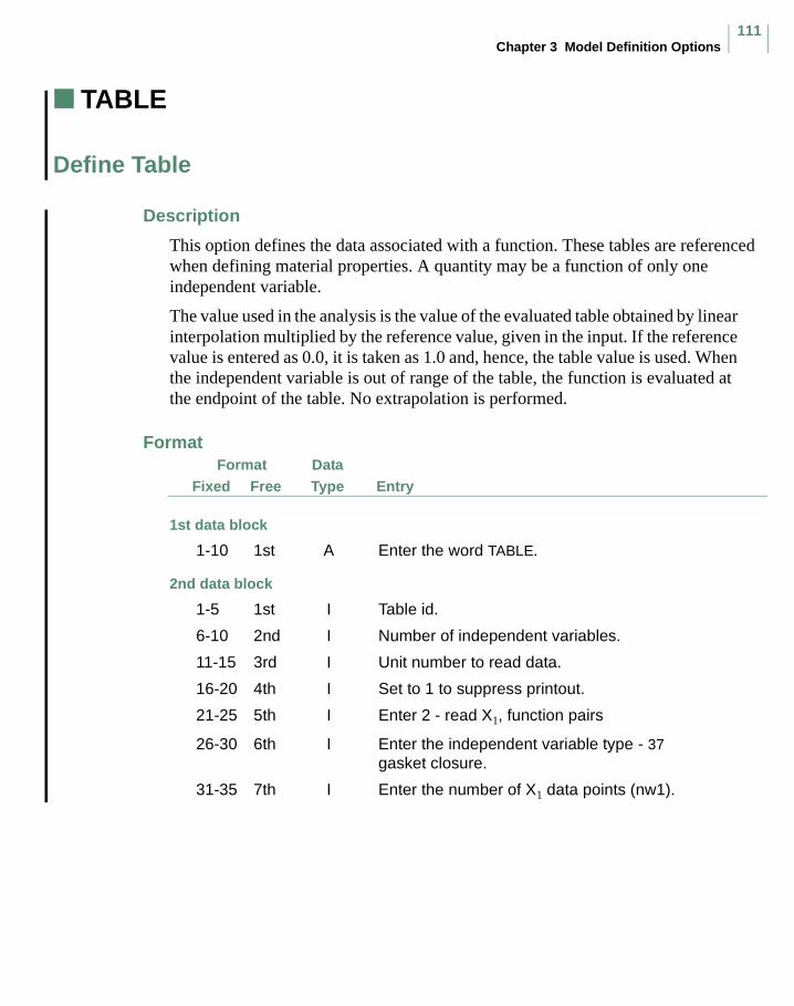
Chapter 3 Model Definition Options111
TABLE
Define Table
Description
This option defines the data associated with a function. These tables are referenced when defining material properties. A quantity may be a function of only one independent variable.
The value used in the analysis is the value of the evaluated table obtained by linear interpolation multiplied by the reference value, given in the input. If the reference value is entered as 0.0, it is taken as 1.0 and, hence, the table value is used. When the independent variable is out of range of the table, the function is evaluated at the endpoint of the table. No extrapolation is performed.
FormatFree Entry
DataTypeFixed
Format
1st data block
1-10 1st A Enter the word TABLE.
2nd data block
1-5 1st I Table id.
6-10 2nd I Number of independent variables.
11-15 3rd I Unit number to read data.
16-20 4th I Set to 1 to suppress printout.
21-25 5th I Enter 2 - read X1, function pairs
26-30 6th I Enter the independent variable type - 37 gasket closure.
31-35 7th I Enter the number of X1 data points (nw1).

MSC.Marc Volume C: Program Input
112
FormatFree Entry
DataTypeFixed
36-40 8th I Not used: enter 0.
41-45 9th I Not used: enter 0.
46-50 10th I Not used: enter 0.
51-55 11th I Not used: enter 0.
56-60 12th I Not used: enter 0.
61-65 13th I Not used: enter 0.
3rd data block
1-32 1st A Enter the table name.
4th data block
Enter nw1 lines each with the value of independent variable and function.
1-10 1st E Enter value of independent variable
11-20 2nd E Enter value of function.

Chapter 3 Model Definition Options113
DAMAGE
Define Properties for Damaging Materials
Description
This option allows you to define a set of data for a specific material which includes a damage model. The specific model and associated data can also be specified with this option.
Gurson Model
For elasto-plastic materials, the damage model is based on a Gurson model for the yield surface definition for materials with voids:
Void nucleation and void growth are based on a model by Tvergaard and Needleman. Here, f* is introduced to model the rapid decrease in load carrying capacity if void coalescence occurs:
if
if
the nucleation can be either stress or strain controlled. The strain controlled nucleation is given by:
Additional data for the initial void volume fraction can be defined with user subroutine UVOID. Other nucleation models are allowed via the user subroutine UVOIDN.
Fσσy-----
22q1f
* q2σkk
2σy-------------
1 q1f*( )
2–[ ]–cosh+ 0= =
f*
f= f fc≤
f*
fc
fu fc–
fF fc–-------------- f fc–( )+= f fc>
f·nucleationfN
S 2π-------------- exp
12---
εpm εn–
S-------------------
2
– ε·pm=

MSC.Marc Volume C: Program Input
114
Rubber Models
For elastomeric materials, the model is based on the undamaged strain energy
function multiplied by a Kachanov damage factor, . The damage capability is available for Ogden strain energy model using the total Lagrange formulation as well as the Mooney-Rivlin, Ogden, and general principal stretch based model using the updated Lagrange formulation.
Both continuous damage (Miehe’s formulation) as well as the discontinuous damage (Mullin’s effect) can be modeled within an additive:
or a multiplicative format:
is automatically calculated by Marc.
Simplified Model
For elastic, elastic-plastic, or rigid-plastic materials, there is the option for you to define a simplified damage model. You define the damage factor (df) in the user subroutine UDAMAG.
If model 9 is used, then:
If model 10 is used, then:
The normal data for a specific material are defined with the ISOTROPIC, WORK HARD, and OGDEN options. Cross-reference to this material is made with the material number.
W°
W K W°⋅=
K d∞ dna
n 1=
N
∑ αηn------–
dmβ
β
λm------–
exp
m 1=
N
∑+exp+= N 1 2,=( )
K d∞ dn expα δnβ+
ηn-------------------–
n 1=
N
∑+= N 1 2,=( )
d∞
σy σy εp ε· p
T, ,( )* 1.0 df–( )=
σy σy εp ε· p
T, ,( )* 1.0 df–( ) and E = E T( )* 1.0 df–( )=
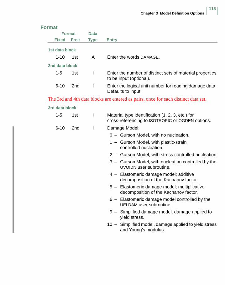
Chapter 3 Model Definition Options115
FormatFree Entry
DataTypeFixed
Format
1st data block
1-10 1st A Enter the words DAMAGE.
2nd data block
1-5 1st I Enter the number of distinct sets of material properties to be input (optional).
6-10 2nd I Enter the logical unit number for reading damage data. Defaults to input.
The 3rd and 4th data blocks are entered as pairs, once for each distinct data set.
3rd data block
1-5 1st I Material type identification (1, 2, 3, etc.) for cross-referencing to ISOTROPIC or OGDEN options.
6-10 2nd I Damage Model:
0 – Gurson Model, with no nucleation.
1 – Gurson Model, with plastic-strain controlled nucleation.
2 – Gurson Model, with stress controlled nucleation.
3 – Gurson Model, with nucleation controlled by the UVOIDN user subroutine.
4 – Elastomeric damage model; additive decomposition of the Kachanov factor.
5 – Elastomeric damage model; multiplicative decomposition of the Kachanov factor.
6 – Elastomeric damage model controlled by the UELDAM user subroutine.
9 – Simplified damage model, damage applied to yield stress.
10 – Simplified model, damage applied to yield stress and Young’s modulus.
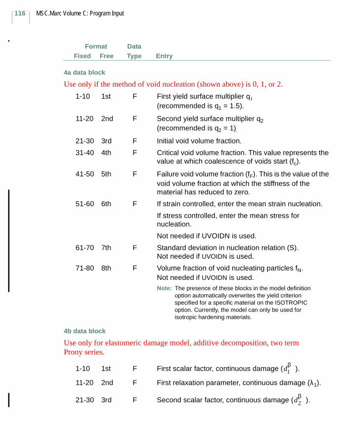
MSC.Marc Volume C: Program Input
116
FormatFree Entry
DataTypeFixed
4a data block
Use only if the method of void nucleation (shown above) is 0, 1, or 2.
1-10 1st F First yield surface multiplier q1
(recommended is q1 = 1.5).
11-20 2nd F Second yield surface multiplier q2
(recommended is q2 = 1).
21-30 3rd F Initial void volume fraction.
31-40 4th F Critical void volume fraction. This value represents the value at which coalescence of voids start (fc).
41-50 5th F Failure void volume fraction (fF). This is the value of the void volume fraction at which the stiffness of the material has reduced to zero.
51-60 6th F If strain controlled, enter the mean strain nucleation.
If stress controlled, enter the mean stress for nucleation.
Not needed if UVOIDN is used.
61-70 7th F Standard deviation in nucleation relation (S).Not needed if UVOIDN is used.
71-80 8th F Volume fraction of void nucleating particles fN.Not needed if UVOIDN is used.Note: The presence of these blocks in the model definition
option automatically overwrites the yield criterion specified for a specific material on the ISOTROPIC option. Currently, the model can only be used for isotropic hardening materials.
4b data block
Use only for elastomeric damage model, additive decomposition, two term Prony series.
1-10 1st F First scalar factor, continuous damage ( ).
11-20 2nd F First relaxation parameter, continuous damage (λ1).
21-30 3rd F Second scalar factor, continuous damage ( ).
dβ1
dβ2
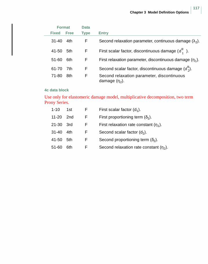
Chapter 3 Model Definition Options117
FormatFree Entry
DataTypeFixed
31-40 4th F Second relaxation parameter, continuous damage (λ2).
41-50 5th F First scalar factor, discontinuous damage ( ).
51-60 6th F First relaxation parameter, discontinuous damage (η1).
61-70 7th F Second scalar factor, discontinuous damage ( ).
71-80 8th F Second relaxation parameter, discontinuous damage (η2).
4c data block
Use only for elastomeric damage model, multiplicative decomposition, two term Prony Series.
1-10 1st F First scalar factor (d1).
11-20 2nd F First proportioning term (δ1).
21-30 3rd F First relaxation rate constant (η1).
31-40 4th F Second scalar factor (d2).
41-50 5th F Second proportioning term (δ2).
51-60 6th F Second relaxation rate constant (η2).
dα1
dα2
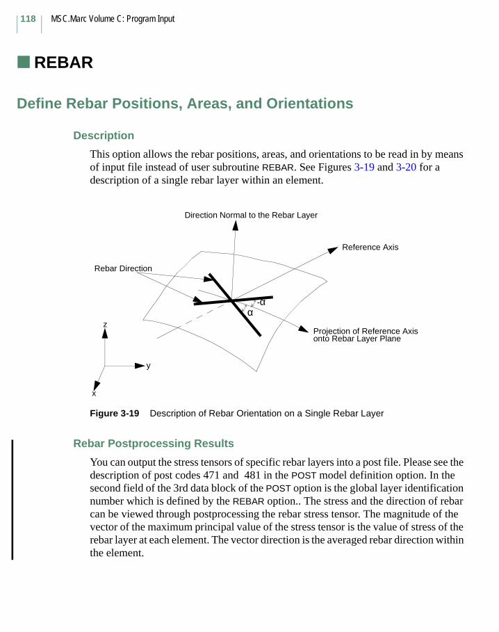
MSC.Marc Volume C: Program Input
118
REBAR
Define Rebar Positions, Areas, and Orientations
Description
This option allows the rebar positions, areas, and orientations to be read in by means of input file instead of user subroutine REBAR. See Figures 3-19 and 3-20 for a description of a single rebar layer within an element.
Figure 3-19 Description of Rebar Orientation on a Single Rebar Layer
Rebar Postprocessing Results
You can output the stress tensors of specific rebar layers into a post file. Please see the description of post codes 471 and 481 in the POST model definition option. In the second field of the 3rd data block of the POST option is the global layer identification number which is defined by the REBAR option.. The stress and the direction of rebar can be viewed through postprocessing the rebar stress tensor. The magnitude of the vector of the maximum principal value of the stress tensor is the value of stress of the rebar layer at each element. The vector direction is the averaged rebar direction within the element.
Rebar Direction
Direction Normal to the Rebar Layer
Reference Axis
Projection of Reference Axisonto Rebar Layer Plane
z
y
x
-αα
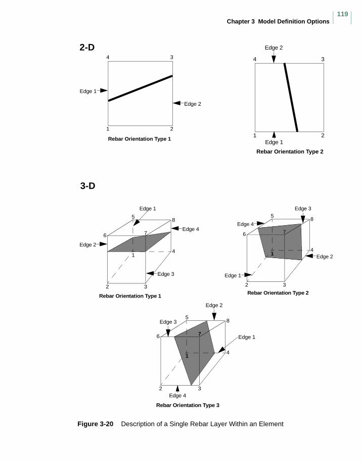
Chapter 3 Model Definition Options119
Figure 3-20 Description of a Single Rebar Layer Within an Element
3-D
4 3
1 2
Edge 1
Edge 2
4 3
1 2
Edge 4
Edge 2
Rebar Orientation Type 1
Edge 3
Rebar Orientation Type 2
Rebar Orientation Type 1
1
2 3
4
5
6 7
8
Edge 4
Edge 1
Edge 2
Edge 1
1
2 3
4
5
6 7
8
Edge 1
Edge 2
Edge 3
Edge 4
Rebar Orientation Type 2
Rebar Orientation Type 3
2 3
4
5
6
8Edge 3
Edge 2
2-D
Edge 1
1
7

MSC.Marc Volume C: Program Input
120
FormatFree Entry
DataTypeFixed
Format
1st data block
1-5 1st A Enter the word REBAR.2nd data block
1-5 1st I Number of data sets to be read in.
6-10 2nd I Unit number for input; defaults to standard input (unit 5).
Data blocks 3, 4, and 5 are given for each data set.3rd data block
1-5 1st I Rebar data set id.
6-10 2nd I Number of rebar layers to be read in. Maximum is 5.
11-15 3rd I Enter 2 if the considered structure is an axisymmetric expansion of cylinders made of bias plies and the cords are nearly inextensible relative to matrix materials. In this case, all parameters below describe the cylinders from which the considered structure was made. The rebar positions, areas, and orientations for real structure is calculated by Marc.When using cylinder expansion option in rebar data definition, the reference axis needs to be the symmetric axis of the original cylinder, and this needs to pass through the origin of the coordinates.
16-25 4th F First direction cosine of reference axis.
26-35 5th F Second direction cosine of reference axis.
36-45 6th F Third direction cosine of reference axis.The default reference axis is (1, 0, 0).Note: (1.) Reference axis should not be perpendicular to
rebar layer.
(2.) If AXITO3D option is used, the reference axis must be (1,0,0). If the rebar layer is vertical to (1,0,0), the program internally switches the reference axis to (0,1,0).
46-50 7th I Enter 0 (default) if no skew type of rebar layers are to be defined.
Enter 2 for 2-D.
Enter 3 for 3-D and for membrane elements. Set to 0 if the third field of the third data block is 2.
Chapter 3 Model Definition Options121
FormatFree Entry
DataTypeFixed
Data block 4 is given for each rebar layer.
4th data block
1-5 1st I Material id.
6-15 2nd F , relative position of the rebar layer at edge 1 (ratio
of the distance between the reference surface (edge) and the rebar layer to the distance across the element); not used for membrane elements.
16-25 3rd F A, area of cross section of each rebar at edge 1.
26-35 4th F S, number of rebars per unit length in each layer at edge 1.Equivalent thickness of the rebar layer is .
36-45 5th F Angle (α) between the rebar and the projection of the reference axis on rebar layer plane [-90, 90] at edge 1. See Figure 3-19.
46-55 6th F Radius of the cylinder; only used when the third field of the 3rd data block is 2.
56-60 7th I Enter the global identification number of the rebar layer. Use for postprocessing only.
61-65 8th I Enter the rebar layer orientation type.
2-D
Enter 1 if this rebar layer is similar to the 1,2 and 3,4 edges of the element; the “thickness” direction is from the 1,2 edge to 3,4 edge of the element.
Enter 2 if this rebar layer is similar to the 1,4 and 2,3 edges of the element; the “thickness” direction is from the 1,4 edge to 2,3 edge of the element.
3-D
Enter 1 if this rebar layer is similar to the 1,2,3,4 and 5,6,7,8 faces of the element; the “thickness” direction is from the 1,2,3,4 face to 5,6,7,8 face of the element.
Enter 2 if this rebar layer is similar to the 1,4,8,5 and 2,3,7,6 faces of the element; the “thickness” direction is from the 1,4,8,5 face to 2,3,7,6 face of the element.
p r ⋅T
------------
A S⋅
MSC.Marc Volume C: Program Input
122
FormatFree Entry
DataTypeFixed
Enter 3 if this rebar layer is similar to the 2,1,5,6 and 3,4,8,7 faces of the element, the “thickness” direction is from the 2,1,5,6 face to 3,4,8,7 face of the element.
Not used for membrane elements.
5th data block is only needed when the 7th field of the third data block is not zero.
5th data block
1-10 1st F Relative position of the rebar layer at edge 2. Not used for membrane elements.
11-20 2nd F Area of cross-section of rebar at edge 2.
21-30 3rd F Number of rebars per unit length at edge 2.
31-40 4th F Angle between the rebar and the projection of the reference axis on rebar layer plane (-90,90) at edge 2.
6th and 7th data blocks are only needed when the 7th field of the third data block is 3.
6th data block
1-10 1st F Relative position of the rebar layer at edge 3. Not used for membrane elements.
11-20 2nd F Area of cross-section of rebar at edge 3.
21-30 3rd F Number of rebars per unit length at edge 3.
31-40 4th F Angle between the rebar and the projection of the reference axis on rebar layer plane (-90,90) at edge 3.
7th data block
1-10 1st F Relative position of the rebar layer at edge 4. Not used for membrane elements.
11-20 2nd F Area of cross-section of rebar at edge 4.
21-30 3rd F Number of rebars per unit length at edge 4.
31-40 4th F Angle between the rebar and the projection of the reference axis on rebar layer plane (-90,90) at edge 4.
8th data block
Enter a list of elements.
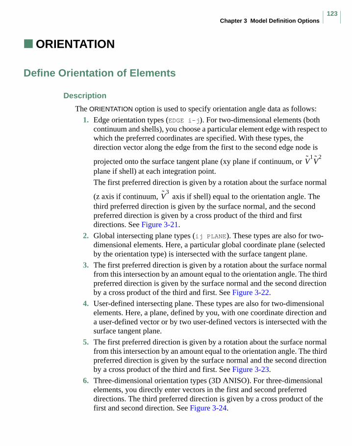
Chapter 3 Model Definition Options123
ORIENTATION
Define Orientation of Elements
Description
The ORIENTATION option is used to specify orientation angle data as follows:
1. Edge orientation types (EDGE i-j). For two-dimensional elements (both continuum and shells), you choose a particular element edge with respect to which the preferred coordinates are specified. With these types, the direction vector along the edge from the first to the second edge node is
projected onto the surface tangent plane (xy plane if continuum, or plane if shell) at each integration point.
The first preferred direction is given by a rotation about the surface normal
(z axis if continuum, axis if shell) equal to the orientation angle. The third preferred direction is given by the surface normal, and the second preferred direction is given by a cross product of the third and first directions. See Figure 3-21.
2. Global intersecting plane types (ij PLANE). These types are also for two-dimensional elements. Here, a particular global coordinate plane (selected by the orientation type) is intersected with the surface tangent plane.
3. The first preferred direction is given by a rotation about the surface normal from this intersection by an amount equal to the orientation angle. The third preferred direction is given by the surface normal and the second direction by a cross product of the third and first. See Figure 3-22.
4. User-defined intersecting plane. These types are also for two-dimensional elements. Here, a plane, defined by you, with one coordinate direction and a user-defined vector or by two user-defined vectors is intersected with the surface tangent plane.
5. The first preferred direction is given by a rotation about the surface normal from this intersection by an amount equal to the orientation angle. The third preferred direction is given by the surface normal and the second direction by a cross product of the third and first. See Figure 3-23.
6. Three-dimensional orientation types (3D ANISO). For three-dimensional elements, you directly enter vectors in the first and second preferred directions. The third preferred direction is given by a cross product of the first and second direction. See Figure 3-24.
V1V
2
V3
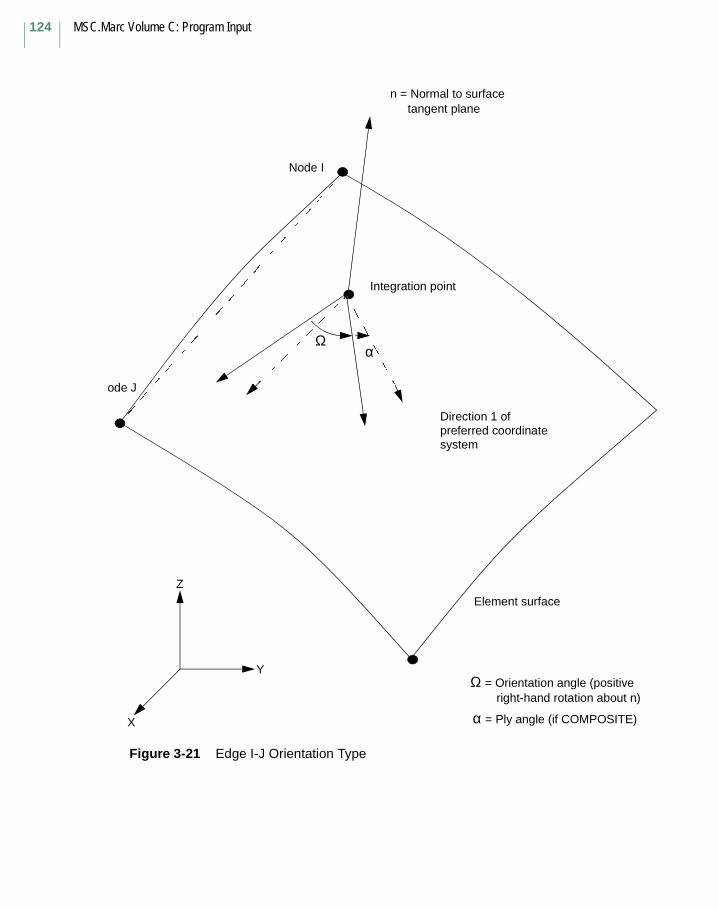
MSC.Marc Volume C: Program Input
124
Figure 3-21 Edge I-J Orientation Type
Ωα
Direction 1 ofpreferred coordinate system
n = Normal to surfacetangent plane
Element surface
Z
Y
X
Ω = Orientation angle (positive
α = Ply angle (if COMPOSITE)
right-hand rotation about n)
Node I
ode J
Integration point
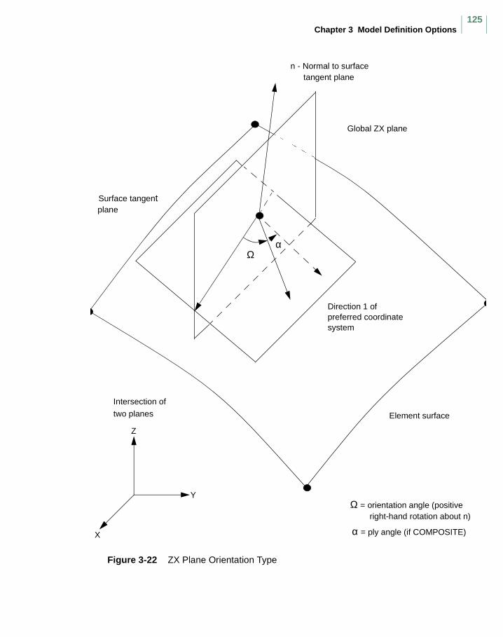
Chapter 3 Model Definition Options125
Figure 3-22 ZX Plane Orientation Type
Ωα
Direction 1 ofpreferred coordinate system
Global ZX plane
n - Normal to surfacetangent plane
Surface tangentplane
Intersection of two planes Element surface
Z
Y
X
Ω = orientation angle (positive
α = ply angle (if COMPOSITE)
right-hand rotation about n)
MSC.Marc Volume C: Program Input
126
Figure 3-23 XU Plane Orientation Type
Ωα
Direction 1 ofpreferred coordinate system
u = User-defined vector
n = Normal to surfacetangent plane
Surface tangentplane
Element surface
Z
Y
X
Ω = Orientation angle (positive
α = ply angle (if COMPOSITE)
right-hand rotation about n)
_
globalX
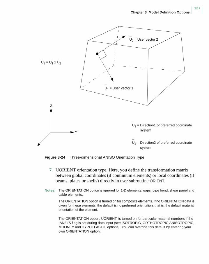
Chapter 3 Model Definition Options127
Figure 3-24 Three-dimensional ANISO Orientation Type
7. UORIENT orientation type. Here, you define the transformation matrix between global coordinates (if continuum elements) or local coordinates (if beams, plates or shells) directly in user subroutine ORIENT.
Notes: The ORIENTATION option is ignored for 1-D elements, gaps, pipe bend, shear panel and cable elements.
The ORIENTATION option is turned on for composite elements. If no ORIENTATION data is given for these elements, the default is no preferred orientation; that is, the default material orientation of the element.
The ORIENTATION option, UORIENT, is turned on for particular material numbers if the IANELS flag is set during data input (see ISOTROPIC, ORTHOTROPIC,ANISOTROPIC, MOONEY and HYPOELASTIC options). You can override this default by entering your own ORIENTATION option.
Z
Y
U1 = Direction1 of preferred coordinatesystem
U2 = Direction2 of preferred coordinatesystem
_
_
U1 = User vector 1
_
U2 = User vector 2
_
U3 = U1 x U2
_ __
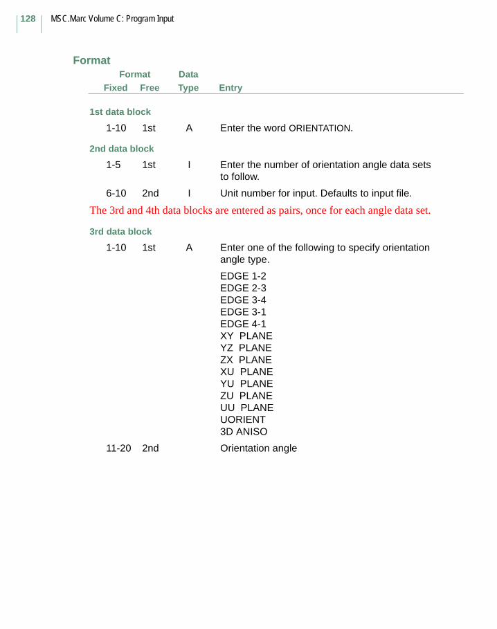
MSC.Marc Volume C: Program Input
128
FormatFree Entry
DataTypeFixed
Format
1st data block
1-10 1st A Enter the word ORIENTATION.
2nd data block
1-5 1st I Enter the number of orientation angle data sets to follow.
6-10 2nd I Unit number for input. Defaults to input file.
The 3rd and 4th data blocks are entered as pairs, once for each angle data set.
3rd data block
1-10 1st A Enter one of the following to specify orientation angle type.
EDGE 1-2EDGE 2-3EDGE 3-4EDGE 3-1EDGE 4-1XY PLANEYZ PLANEZX PLANEXU PLANEYU PLANEZU PLANEUU PLANEUORIENT3D ANISO
11-20 2nd Orientation angle

Chapter 3 Model Definition Options129
FormatFree Entry
DataTypeFixed
For XU PLANE, YU PLANE, ZU PLANE, UU PLANE, and 3D ANISO, complete the following:
21-30 3rd F 1
31-40 4th F 2 component of user vector 1 w.r.t. global coordinates.
41-50 5th F 3
For UU PLANE and 3D ANISO, complete the following:
51-60 6th F 1
61-70 7th F 2 component of user vector 2 w.r.t. global coordinates.
71-80 8th F 3
4th data block
Enter a list of elements to be associated with this orientation angle.
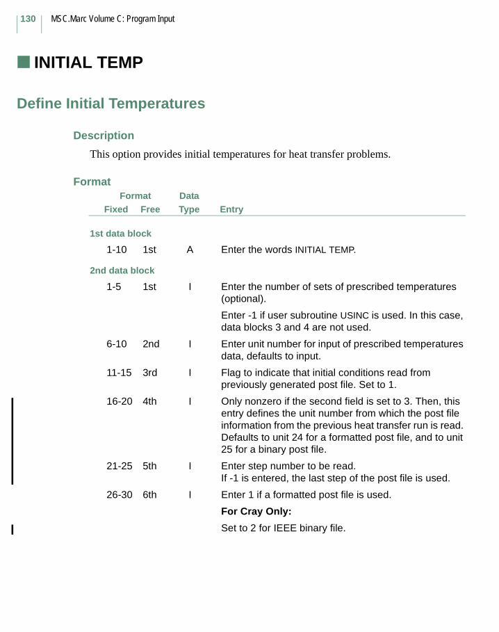
MSC.Marc Volume C: Program Input
130
INITIAL TEMP (Heat Transfer)
Define Initial Temperatures
Description
This option provides initial temperatures for heat transfer problems.
FormatFree Entry
DataTypeFixed
Format
1st data block
1-10 1st A Enter the words INITIAL TEMP.
2nd data block
1-5 1st I Enter the number of sets of prescribed temperatures (optional).
Enter -1 if user subroutine USINC is used. In this case, data blocks 3 and 4 are not used.
6-10 2nd I Enter unit number for input of prescribed temperatures data, defaults to input.
11-15 3rd I Flag to indicate that initial conditions read from previously generated post file. Set to 1.
16-20 4th I Only nonzero if the second field is set to 3. Then, this entry defines the unit number from which the post file information from the previous heat transfer run is read. Defaults to unit 24 for a formatted post file, and to unit 25 for a binary post file.
21-25 5th I Enter step number to be read. If -1 is entered, the last step of the post file is used.
26-30 6th I Enter 1 if a formatted post file is used.
For Cray Only:
Set to 2 for IEEE binary file.
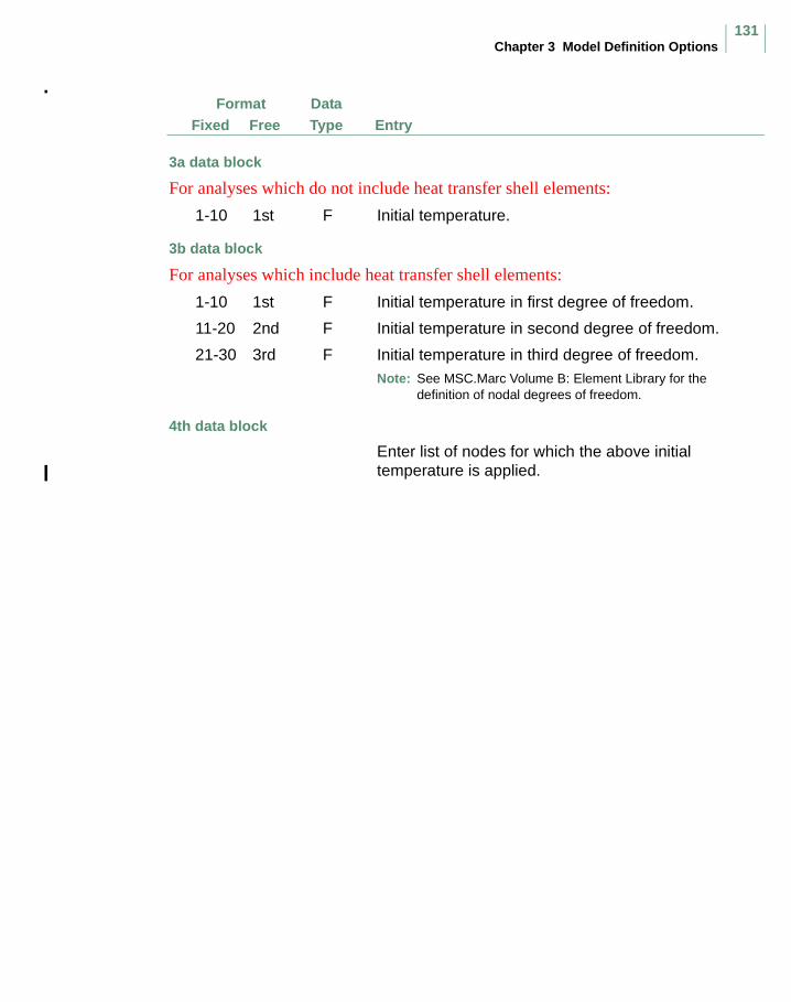
Chapter 3 Model Definition Options131
FormatFree Entry
DataTypeFixed
3a data block
For analyses which do not include heat transfer shell elements:
1-10 1st F Initial temperature.
3b data block
For analyses which include heat transfer shell elements:
1-10 1st F Initial temperature in first degree of freedom.
11-20 2nd F Initial temperature in second degree of freedom.
21-30 3rd F Initial temperature in third degree of freedom.Note: See MSC.Marc Volume B: Element Library for the
definition of nodal degrees of freedom.
4th data block
Enter list of nodes for which the above initial temperature is applied.

MSC.Marc Volume C: Program Input
132
Chapter 4 History Definition
Options

Chapter 4 History Definition Options133
NEW (History Definition)
Use New Format
Description
This option allows the input of data in the K style format. Input is interpreted to be in this format until an OLD option is encountered. This option must not appear embedded inside a model definition or history definition option.
FormatFree Entry
DataTypeFixed
Format
1-10 1st A Enter the word NEW.
11-15 2nd I Enter 1 if the default width of the data fields is used for input.This will override the EXTENDED parameter.
Enter 2 if the double width of the data fields is used for input.
MSC.Marc Volume C: Program Input
134
OLD (History Definition)
Use Old Format
Description
This option allows the input of data in the old (G, H, or J) style format. Input is interpreted to be in this format until a NEW option is encountered. This option must not appear embedded inside a model definition or history definition option.
FormatFree Entry
DataTypeFixed
Formats
1-10 1st A Enter the word OLD.
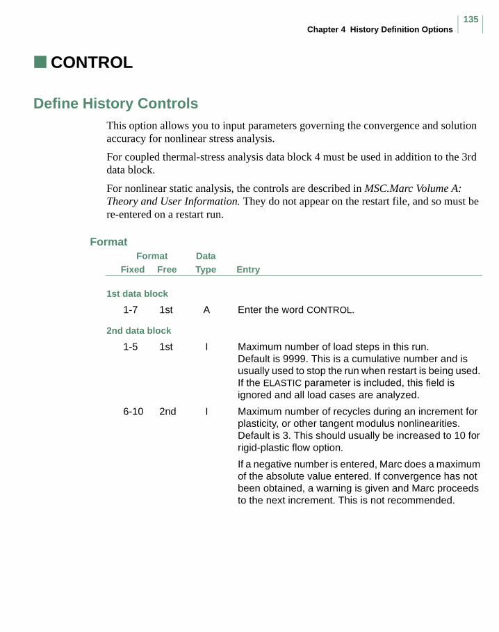
Chapter 4 History Definition Options135
CONTROL (Stress)
Define History ControlsThis option allows you to input parameters governing the convergence and solution accuracy for nonlinear stress analysis.
For coupled thermal-stress analysis data block 4 must be used in addition to the 3rd data block.
For nonlinear static analysis, the controls are described in MSC.Marc Volume A: Theory and User Information. They do not appear on the restart file, and so must be re-entered on a restart run.
FormatFree Entry
DataTypeFixed
Format
1st data block
1-7 1st A Enter the word CONTROL.
2nd data block
1-5 1st I Maximum number of load steps in this run. Default is 9999. This is a cumulative number and is usually used to stop the run when restart is being used. If the ELASTIC parameter is included, this field is ignored and all load cases are analyzed.
6-10 2nd I Maximum number of recycles during an increment for plasticity, or other tangent modulus nonlinearities. Default is 3. This should usually be increased to 10 for rigid-plastic flow option.
If a negative number is entered, Marc does a maximum of the absolute value entered. If convergence has not been obtained, a warning is given and Marc proceeds to the next increment. This is not recommended.

MSC.Marc Volume C: Program Input
136
FormatFree Entry
DataTypeFixed
11-15 3rd I Minimum number of recycles during an increment for plasticity or other tangent modulus nonlinearities. Default is 0. Note: This data field forces this number of recycles to take
place at all subsequent increments. CAUTION: This value is overwritten by the PROPORTIONAL
INCREMENT option.
16-20 4th I Flag for convergence testing. 0 or left blank Convergence is achieved when
residuals satisfy the criteria. 1 Convergence is achieved when
displacements satisfy the criteria.2 Convergence is achieved when strain
energy satisfies the criteria.4 Convergence is achieved when either
residual or displacement satisfies the criterion.
5 Convergence is achieved when both residual and displacement satisfies the criterion.
Notes: Testing on relative displacements or strain energy always requires at least one iteration. If nonlinear analysis is done with the CENTROID parameter, the residuals are not calculated and testing is always done on displacements.
Nonlinear analysis with the CENTROID parameter is not recommended. If the fields are set as 0, 1, or 2, only the 3rd data block is needed.If the fields are set as 4 or 5, the 3a data block is also needed. In this case, the 3rd data block is set for residual testing and 3a data block is set for displacements check only.
21-25 5th I Flag to specify relative or absolute error testing.If equal to 0 Testing is done on relative error. If equal to 1 Testing is done on absolute value.
If set to 2 Testing is done on relative error testing unless reactions or incremental displacements are below minimum value in which case absolute tolerances testing is used.
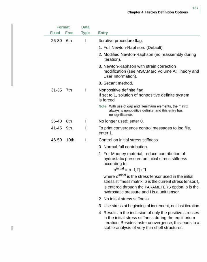
Chapter 4 History Definition Options137
FormatFree Entry
DataTypeFixed
26-30 6th I Iterative procedure flag.
1. Full Newton-Raphson. (Default)
2. Modified Newton-Raphson (no reassembly during iteration).
3. Newton-Raphson with strain correction modification (see MSC.Marc Volume A: Theory and User Information).
8. Secant method.
31-35 7th I Nonpositive definite flag. If set to 1, solution of nonpositive definite system is forced. Note: With use of gap and Herrmann elements, the matrix
always is nonpositive definite, and this entry has no significance.
36-40 8th I No longer used; enter 0.
41-45 9th I To print convergence control messages to log file, enter 1.
46-50 10th I Control on initial stress stiffness
0 Normal-full contribution.
1 For Mooney material, reduce contribution of hydrostatic pressure on initial stress stiffness according to:
σinitial = σ -fr ⋅ p ⋅ Iwhere σinitial is the stress tensor used in the initial stress stiffness matrix, σ is the current stress tensor, fr is entered through the PARAMETERS option, p is the hydrostatic pressure and I is a unit tensor.
2 No initial stress stiffness.
3 Use stress at beginning of increment, not last iteration.
4 Results in the inclusion of only the positive stresses in the initial stress stiffness during the equilibrium iteration. Besides faster convergence, this leads to a stable analysis of very thin shell structures.
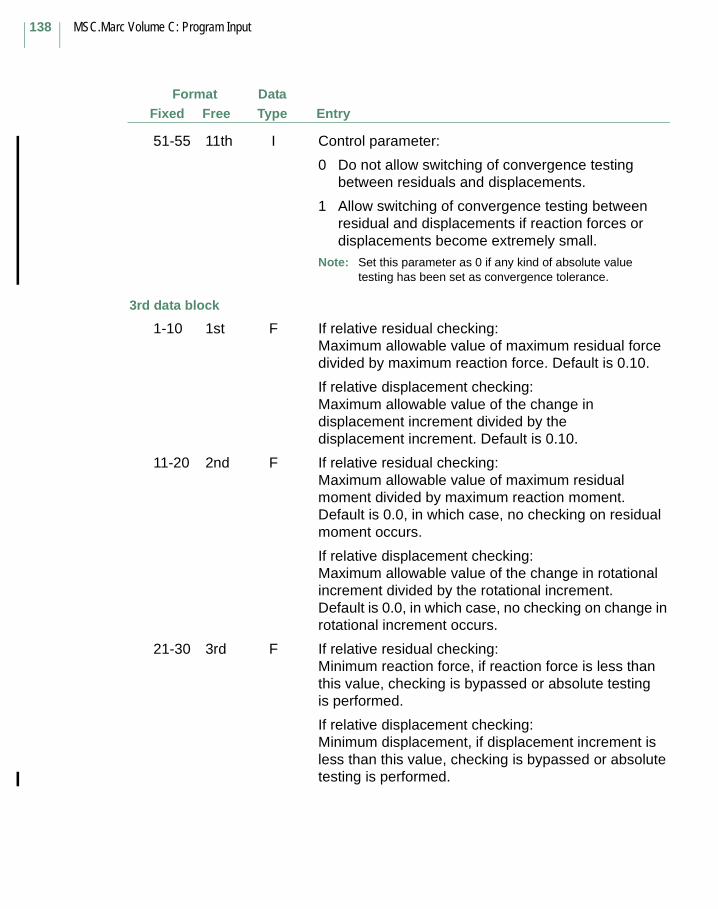
MSC.Marc Volume C: Program Input
138
FormatFree Entry
DataTypeFixed
51-55 11th I Control parameter:
0 Do not allow switching of convergence testing between residuals and displacements.
1 Allow switching of convergence testing between residual and displacements if reaction forces or displacements become extremely small.
Note: Set this parameter as 0 if any kind of absolute value testing has been set as convergence tolerance.
3rd data block
1-10 1st F If relative residual checking: Maximum allowable value of maximum residual force divided by maximum reaction force. Default is 0.10.
If relative displacement checking: Maximum allowable value of the change in displacement increment divided by the displacement increment. Default is 0.10.
11-20 2nd F If relative residual checking: Maximum allowable value of maximum residual moment divided by maximum reaction moment. Default is 0.0, in which case, no checking on residual moment occurs.
If relative displacement checking: Maximum allowable value of the change in rotational increment divided by the rotational increment. Default is 0.0, in which case, no checking on change in rotational increment occurs.
21-30 3rd F If relative residual checking: Minimum reaction force, if reaction force is less than this value, checking is bypassed or absolute testing is performed.
If relative displacement checking: Minimum displacement, if displacement increment is less than this value, checking is bypassed or absolute testing is performed.
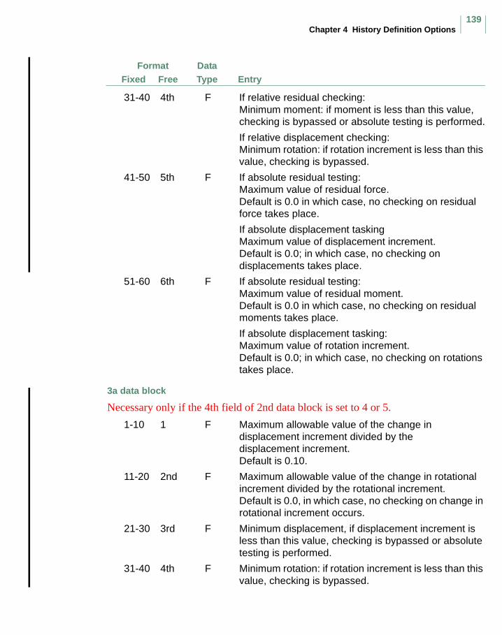
Chapter 4 History Definition Options139
FormatFree Entry
DataTypeFixed
31-40 4th F If relative residual checking: Minimum moment: if moment is less than this value, checking is bypassed or absolute testing is performed.
If relative displacement checking: Minimum rotation: if rotation increment is less than this value, checking is bypassed.
41-50 5th F If absolute residual testing:Maximum value of residual force. Default is 0.0 in which case, no checking on residual force takes place.
If absolute displacement taskingMaximum value of displacement increment.Default is 0.0; in which case, no checking on displacements takes place.
51-60 6th F If absolute residual testing:Maximum value of residual moment. Default is 0.0 in which case, no checking on residual moments takes place.
If absolute displacement tasking:Maximum value of rotation increment.Default is 0.0; in which case, no checking on rotations takes place.
3a data block
Necessary only if the 4th field of 2nd data block is set to 4 or 5.
1-10 1 F Maximum allowable value of the change in displacement increment divided by the displacement increment. Default is 0.10.
11-20 2nd F Maximum allowable value of the change in rotational increment divided by the rotational increment. Default is 0.0, in which case, no checking on change in rotational increment occurs.
21-30 3rd F Minimum displacement, if displacement increment is less than this value, checking is bypassed or absolute testing is performed.
31-40 4th F Minimum rotation: if rotation increment is less than this value, checking is bypassed.
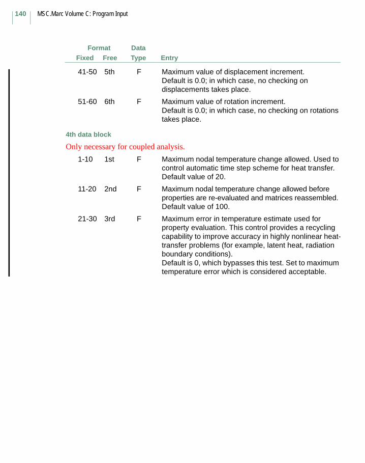
MSC.Marc Volume C: Program Input
140
FormatFree Entry
DataTypeFixed
41-50 5th F Maximum value of displacement increment.Default is 0.0; in which case, no checking on displacements takes place.
51-60 6th F Maximum value of rotation increment.Default is 0.0; in which case, no checking on rotations takes place.
4th data block
Only necessary for coupled analysis.
1-10 1st F Maximum nodal temperature change allowed. Used to control automatic time step scheme for heat transfer. Default value of 20.
11-20 2nd F Maximum nodal temperature change allowed before properties are re-evaluated and matrices reassembled. Default value of 100.
21-30 3rd F Maximum error in temperature estimate used for property evaluation. This control provides a recycling capability to improve accuracy in highly nonlinear heat-transfer problems (for example, latent heat, radiation boundary conditions). Default is 0, which bypasses this test. Set to maximum temperature error which is considered acceptable.

Chapter 4 History Definition Options141
PARAMETERS (History Definition)
Definition of Parameters used in Numerical Analysis
Description
There are many parameters that are used in the finite element calculations. These parameters can be customized for your particular application. Some of these constants can be entered in other input blocks as well. The last nonzero value is used for the calculation.
FormatFree Entry
DataTypeFixed
Format
1st data block
1-10 1st A Enter the word PARAMETERS.
2nd data block
1-10 1st E Enter the scale factor which, when multiplied with the incremental strain, is used to predict the incremental strain in the next increment.Default is 1.0.
11-20 2nd E Enter the multiplier used to calculate the penalty used to impose boundary conditions.Default is 1.e9.The penalty used is, hence, 1.e9 times the maximum diagonal of the stiffness matrix. If the APPBC parameter is used, this option is not used.
21-30 3rd E Enter the penalty factor used to satisfy incompressibility in rigid plastic analysis for plane strain, axisymmetric, or solid analysis when displacement elements are used.Default is 100.
31-40 4th E Enter the penalty factor used to satisfy incompressibility in fluid analysis when displacement elements are used.Default is 1.e6.
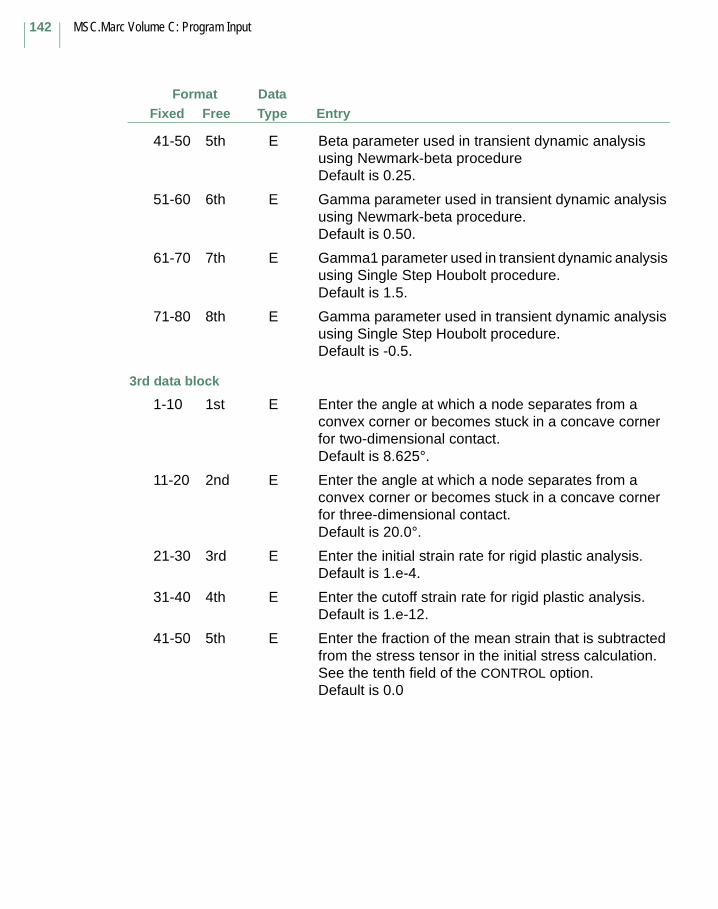
MSC.Marc Volume C: Program Input
142
FormatFree Entry
DataTypeFixed
41-50 5th E Beta parameter used in transient dynamic analysis using Newmark-beta procedureDefault is 0.25.
51-60 6th E Gamma parameter used in transient dynamic analysis using Newmark-beta procedure.Default is 0.50.
61-70 7th E Gamma1 parameter used in transient dynamic analysis using Single Step Houbolt procedure.Default is 1.5.
71-80 8th E Gamma parameter used in transient dynamic analysis using Single Step Houbolt procedure.Default is -0.5.
3rd data block
1-10 1st E Enter the angle at which a node separates from a convex corner or becomes stuck in a concave corner for two-dimensional contact.Default is 8.625°.
11-20 2nd E Enter the angle at which a node separates from a convex corner or becomes stuck in a concave corner for three-dimensional contact.Default is 20.0°.
21-30 3rd E Enter the initial strain rate for rigid plastic analysis.Default is 1.e-4.
31-40 4th E Enter the cutoff strain rate for rigid plastic analysis.Default is 1.e-12.
41-50 5th E Enter the fraction of the mean strain that is subtracted from the stress tensor in the initial stress calculation. See the tenth field of the CONTROL option.Default is 0.0
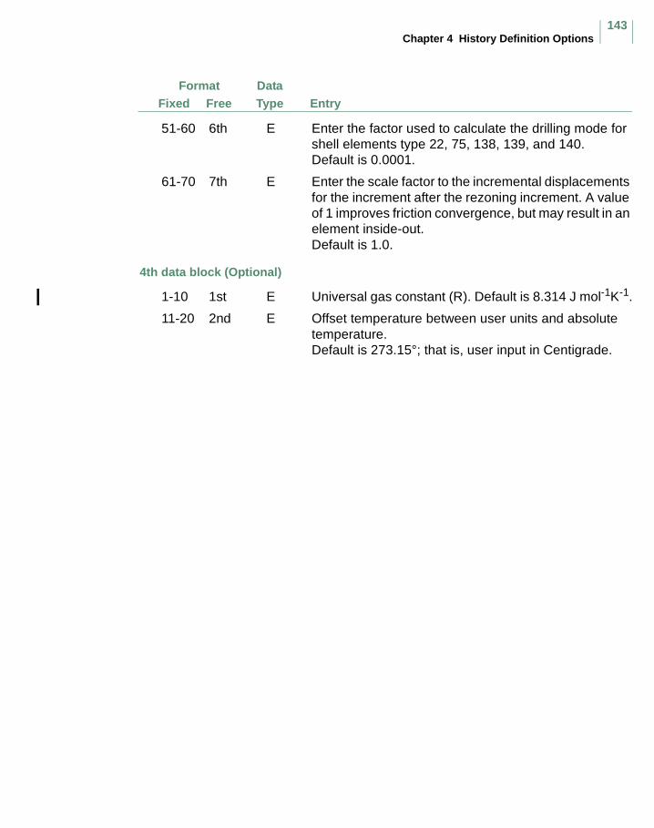
Chapter 4 History Definition Options143
FormatFree Entry
DataTypeFixed
51-60 6th E Enter the factor used to calculate the drilling mode for shell elements type 22, 75, 138, 139, and 140.Default is 0.0001.
61-70 7th E Enter the scale factor to the incremental displacements for the increment after the rezoning increment. A value of 1 improves friction convergence, but may result in an element inside-out.Default is 1.0.
4th data block (Optional)
1-10 1st E Universal gas constant (R). Default is 8.314 J mol-1K-1.
11-20 2nd E Offset temperature between user units and absolute temperature. Default is 273.15°; that is, user input in Centigrade.
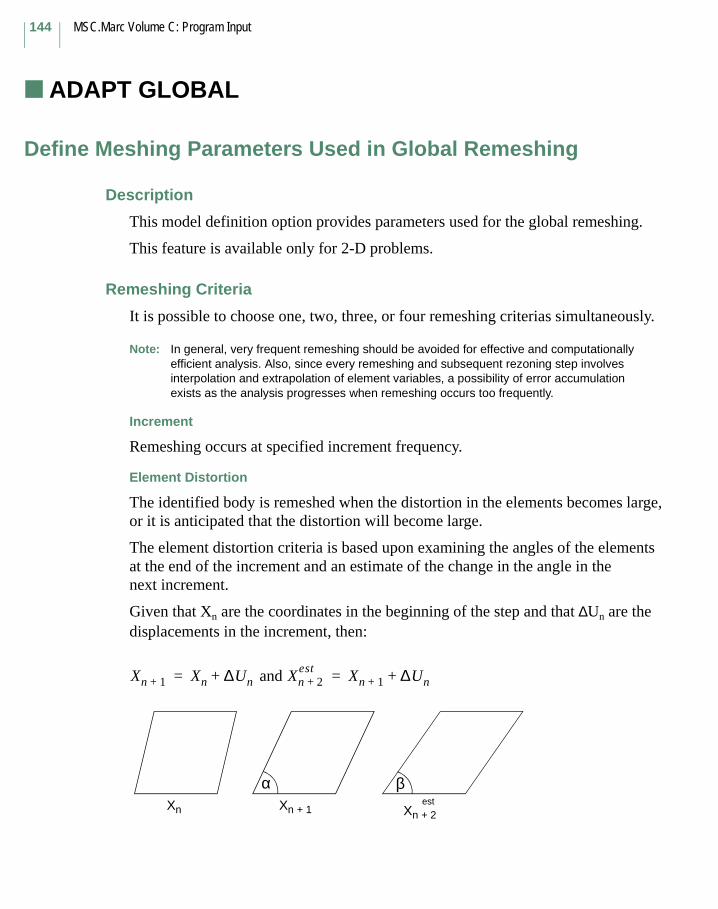
MSC.Marc Volume C: Program Input
144
ADAPT GLOBAL (History Definition)
Define Meshing Parameters Used in Global Remeshing
Description
This model definition option provides parameters used for the global remeshing.
This feature is available only for 2-D problems.
Remeshing Criteria
It is possible to choose one, two, three, or four remeshing criterias simultaneously.
Note: In general, very frequent remeshing should be avoided for effective and computationally efficient analysis. Also, since every remeshing and subsequent rezoning step involves interpolation and extrapolation of element variables, a possibility of error accumulation exists as the analysis progresses when remeshing occurs too frequently.
Increment
Remeshing occurs at specified increment frequency.
Element Distortion
The identified body is remeshed when the distortion in the elements becomes large, or it is anticipated that the distortion will become large.
The element distortion criteria is based upon examining the angles of the elements at the end of the increment and an estimate of the change in the angle in the next increment.
Given that Xn are the coordinates in the beginning of the step and that ∆Un are the displacements in the increment, then:
and Xn 1+ Xn ∆Un+= Xn 2+est Xn 1+ ∆Un+=
Xn Xn + 1 Xn + 2est
α β

Chapter 4 History Definition Options145
If cos α > 0.8 and cos β > 0.9, remesh, or if cos α > 0.9 and cos β > cos α, remesh
which is equivalent to
0 <α < 36° and 0<β<25° remesh or144°<α<180° and 155°<β<180° remesh or0<α<25° and β<α or155°<α<180° and β>α
Contact Penetration
The identified body is remeshed when the curvature of the contact body is such that the current mesh cannot accurately detect penetration.
The penetration remeshing criteria is based upon examining the distance between the edge of the element and the representation of the other contact surface.
If b> penetration limit, remeshing is required. By default, penetration is 2 * (contact tolerance). The contact tolerance can be input by you or computed internally by the program
Please note that this check does not apply to the self-contact situation.
Angle Deviation
The identified body remeshes when the angles in the element have a deviation from the ideal angle greater than a specified amount. The ideal angle for quadrilaterals or hexahedrals is 90°. The ideal angle for triangles and tetrahedrals is 60°. The default of 40° indicates that any angle in the range 50< α < 130 is acceptable for quadrilaterals.
Immediate
The identified body is remeshed before performing any analysis.
b

MSC.Marc Volume C: Program Input
146
FormatFree Entry
DataTypeFixed
Format
1st data block
1-8 1st A Enter the words ADAPT GLOBAL.
2nd data block
1-5 1st I Enter the number of bodies to be remeshed.
6-10 2nd I Enter 0 for default.Enter the unit number to read data; defaults to input.
11-15 3rd I Not used; enter 0.
The third, fourth, and fifth data blocks are repeated as a set for each criteria selected based on the number of remeshing bodies selected in the 2nd data block.
3rd data block
1-5 1st I Enter 2 for Advancing Front 2-D quadrilateral or triangular mesher.
Enter 3 for Delaunay 2-D triangular mesher
Enter 4 for 2-D Overlay quadrilateral mesher.
A valid mesher type (2-4) must be used.
6-10 2nd I Not used; enter 0.
11-15 3rd I Enter the contact body to be remeshed (default = 1) where the contact body number is defined under the CONTACT option.
4th data block
1-5 1st I Enter 1 if increment frequency used as remesh criterion.
6-10 2nd I Enter 1 if element distortion used as remesh criterion.
11-15 3rd I Enter 1 if penetration is used as remesh criterion.
16-20 4th I If the first field is 1, enter the frequency in increments.
21-30 5th E Not used.
31-35 6th I Enter 1 if angle criterion is used.
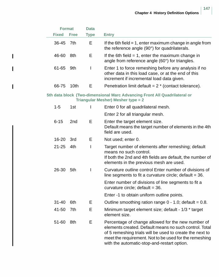
Chapter 4 History Definition Options147
FormatFree Entry
DataTypeFixed
36-45 7th E If the 6th field = 1, enter maximum change in angle from the reference angle (90°) for quadrilaterals.
46-60 8th E If the 6th field = 1, enter the maximum change in angle from reference angle (60°) for triangles.
61-65 9th I Enter 1 to force remeshing before any analysis if no other data in this load case, or at the end of this increment if incremental load data given.
66-75 10th E Penetration limit default = 2 * (contact tolerance).
5th data block (Two-dimensional Marc Advancing Front All Quadrilateral or Triangular Mesher) Mesher type = 2
1-5 1st I Enter 0 for all quadrilateral mesh.
Enter 2 for all triangular mesh.
6-15 2nd E Enter the target element size.Default means the target number of elements in the 4th field are used.
16-20 3rd E Not used; enter 0.
21-25 4th I Target number of elements after remeshing; default means no such control.If both the 2nd and 4th fields are default, the number of elements in the previous mesh are used.
26-30 5th I Curvature outline control Enter number of divisions of line segments to fit a curvature circle; default = 36.
Enter number of divisions of line segments to fit a curvature circle; default = 36.
Enter -1 to obtain uniform outline points.
31-40 6th E Outline smoothing ration range 0 - 1.0; default = 0.8.
41-50 7th E Minimum target element size; default - 1/3 * target element size.
51-60 8th E Percentage of change allowed for the new number of elements created. Default means no such control. Total of 5 remeshing trials will be used to create the next to meet the requirement. Not to be used for the remeshing with the automatic-stop-and-restart option.
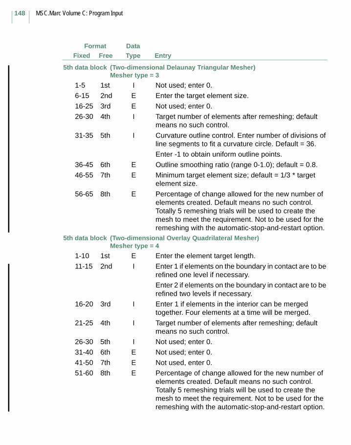
MSC.Marc Volume C: Program Input
148
FormatFree Entry
DataTypeFixed
5th data block (Two-dimensional Delaunay Triangular Mesher)Mesher type = 3
1-5 1st I Not used; enter 0.
6-15 2nd E Enter the target element size.
16-25 3rd E Not used; enter 0.
26-30 4th I Target number of elements after remeshing; default means no such control.
31-35 5th I Curvature outline control. Enter number of divisions of line segments to fit a curvature circle. Default = 36.
Enter -1 to obtain uniform outline points.
36-45 6th E Outline smoothing ratio (range 0-1.0); default = 0.8.
46-55 7th E Minimum target element size; default = 1/3 * target element size.
56-65 8th E Percentage of change allowed for the new number of elements created. Default means no such control. Totally 5 remeshing trials will be used to create the mesh to meet the requirement. Not to be used for the remeshing with the automatic-stop-and-restart option.
5th data block (Two-dimensional Overlay Quadrilateral Mesher)Mesher type = 4
1-10 1st E Enter the element target length.
11-15 2nd I Enter 1 if elements on the boundary in contact are to be refined one level if necessary.
Enter 2 if elements on the boundary in contact are to be refined two levels if necessary.
16-20 3rd I Enter 1 if elements in the interior can be merged together. Four elements at a time will be merged.
21-25 4th I Target number of elements after remeshing; default means no such control.
26-30 5th I Not used; enter 0.
31-40 6th E Not used; enter 0.
41-50 7th E Not used, enter 0.
51-60 8th E Percentage of change allowed for the new number of elements created. Default means no such control. Totally 5 remeshing trials will be used to create the mesh to meet the requirement. Not to be used for the remeshing with the automatic-stop-and-restart option.
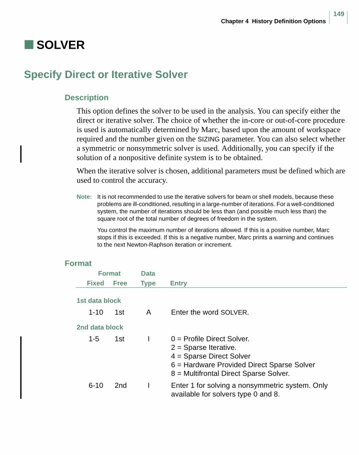
Chapter 4 History Definition Options149
SOLVER (History Definition)
Specify Direct or Iterative Solver
Description
This option defines the solver to be used in the analysis. You can specify either the direct or iterative solver. The choice of whether the in-core or out-of-core procedure is used is automatically determined by Marc, based upon the amount of workspace required and the number given on the SIZING parameter. You can also select whether a symmetric or nonsymmetric solver is used. Additionally, you can specify if the solution of a nonpositive definite system is to be obtained.
When the iterative solver is chosen, additional parameters must be defined which are used to control the accuracy.
Note: It is not recommended to use the iterative solvers for beam or shell models, because these problems are ill-conditioned, resulting in a large-number of iterations. For a well-conditioned system, the number of iterations should be less than (and possible much less than) the square root of the total number of degrees of freedom in the system.
You control the maximum number of iterations allowed. If this is a positive number, Marc stops if this is exceeded. If this is a negative number, Marc prints a warning and continues to the next Newton-Raphson iteration or increment.
FormatFree Entry
DataTypeFixed
Format
1st data block
1-10 1st A Enter the word SOLVER.
2nd data block
1-5 1st I 0 = Profile Direct Solver.2 = Sparse Iterative.4 = Sparse Direct Solver6 = Hardware Provided Direct Sparse Solver8 = Multifrontal Direct Sparse Solver.
6-10 2nd I Enter 1 for solving a nonsymmetric system. Only available for solvers type 0 and 8.
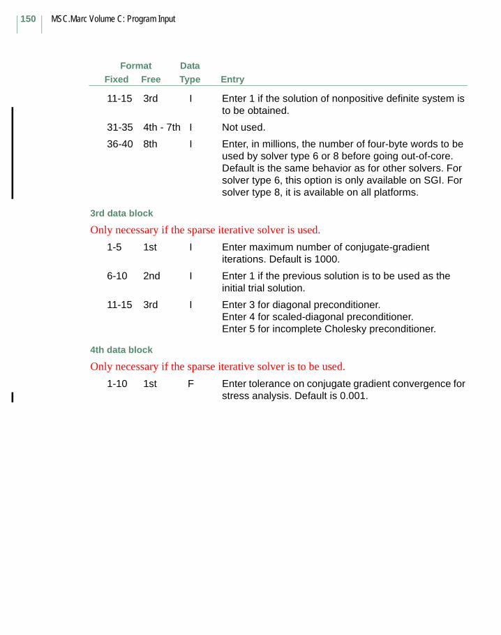
MSC.Marc Volume C: Program Input
150
FormatFree Entry
DataTypeFixed
11-15 3rd I Enter 1 if the solution of nonpositive definite system is to be obtained.
31-35 4th - 7th I Not used.
36-40 8th I Enter, in millions, the number of four-byte words to be used by solver type 6 or 8 before going out-of-core. Default is the same behavior as for other solvers. For solver type 6, this option is only available on SGI. For solver type 8, it is available on all platforms.
3rd data block
Only necessary if the sparse iterative solver is used.
1-5 1st I Enter maximum number of conjugate-gradient iterations. Default is 1000.
6-10 2nd I Enter 1 if the previous solution is to be used as the initial trial solution.
11-15 3rd I Enter 3 for diagonal preconditioner.Enter 4 for scaled-diagonal preconditioner.Enter 5 for incomplete Cholesky preconditioner.
4th data block
Only necessary if the sparse iterative solver is to be used.
1-10 1st F Enter tolerance on conjugate gradient convergence for stress analysis. Default is 0.001.
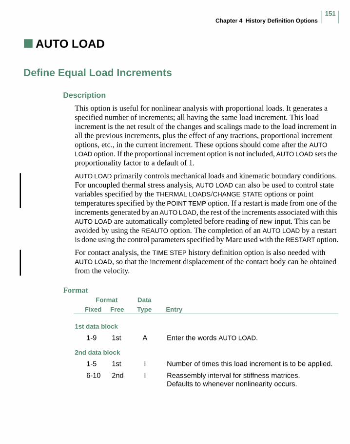
Chapter 4 History Definition Options151
AUTO LOAD
Define Equal Load Increments
Description
This option is useful for nonlinear analysis with proportional loads. It generates a specified number of increments; all having the same load increment. This load increment is the net result of the changes and scalings made to the load increment in all the previous increments, plus the effect of any tractions, proportional increment options, etc., in the current increment. These options should come after the AUTO LOAD option. If the proportional increment option is not included, AUTO LOAD sets the proportionality factor to a default of 1.
AUTO LOAD primarily controls mechanical loads and kinematic boundary conditions. For uncoupled thermal stress analysis, AUTO LOAD can also be used to control state variables specified by the THERMAL LOADS/CHANGE STATE options or point temperatures specified by the POINT TEMP option. If a restart is made from one of the increments generated by an AUTO LOAD, the rest of the increments associated with this AUTO LOAD are automatically completed before reading of new input. This can be avoided by using the REAUTO option. The completion of an AUTO LOAD by a restart is done using the control parameters specified by Marc used with the RESTART option.
For contact analysis, the TIME STEP history definition option is also needed with AUTO LOAD, so that the increment displacement of the contact body can be obtained from the velocity.
FormatFree Entry
DataTypeFixed
Format
1st data block
1-9 1st A Enter the words AUTO LOAD.
2nd data block
1-5 1st I Number of times this load increment is to be applied.
6-10 2nd I Reassembly interval for stiffness matrices. Defaults to whenever nonlinearity occurs.

MSC.Marc Volume C: Program Input
152
FormatFree Entry
DataTypeFixed
11-15 3rd I Maximum number of allowable time step cuts.
= 0 means no automatic restart from the previously converged step.
> 1 means maximum number of time step cutbacks allowed. Marc automatically restart the analysis after each cutback until the maximum number is reached.

Chapter 4 History Definition Options153
AUTO INCREMENT
Define Automatic Load Stepping
Description
This option allows automatic load stepping in a quasi-static analysis and is very useful for both geometric (LARGE DISP) and material (elastic-plastic) nonlinear problems. The option is capable of handling elastic/plastic snap-through phenomena; hence, the post-buckling behavior of structures can be analyzed. However, the option cannot be used for thermal loading.
You have to specify in the DIST LOADS, POINT LOAD, and/or DISP CHANGE options the total loading for a sequence of load steps, and Marc automatically generates the magnitude of each load step based on an initial load step and the amount of nonlinearity occurring during the loading.
The length of the incremental displacement vector (C = ∆uT∆u) is based on the number of recycles in the previous increment. The size of the load increment is controlled by the length of the incremental displacement vector. The analysis is stopped when the total load is reached or when the maximum allowed number of increments is reached. In case of a snap-through problem, the loading can initially increase, decrease after the buckle load has been reached, and increase if the stiffness increases in the post-buckled state. Within the history definition data, the AUTO INCREMENT option can be used as often as desired. For more details, see MSC.Marc Volume A: Theory and User Information.
Notes: The option cannot be used for thermal loading; use the AUTO THERM option instead.
If this option is used for post-buckling analysis, the nonpositive definite flag in the SOLVER model definition option has to be used. This option can be added upon restart.
FormatFree Entry
DataTypeFixed
Format
1st data block
1-14 1st A Enter the words AUTO INCREMENT.
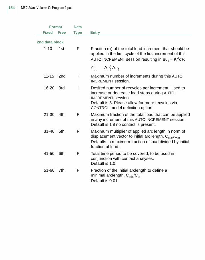
MSC.Marc Volume C: Program Input
154
FormatFree Entry
DataTypeFixed
2nd data block
1-10 1st F Fraction (α) of the total load increment that should be applied in the first cycle of the first increment of this AUTO INCREMENT session resulting in ∆u1 = K-1αP.
.
11-15 2nd I Maximum number of increments during this AUTO INCREMENT session.
16-20 3rd I Desired number of recycles per increment. Used to increase or decrease load steps during AUTO INCREMENT session. Default is 3. Please allow for more recycles via CONTROL model definition option.
21-30 4th F Maximum fraction of the total load that can be applied in any increment of this AUTO INCREMENT session. Default is 1 if no contact is present.
31-40 5th F Maximum multiplier of applied arc length in norm of displacement vector to initial arc length. Cmax/Cin
Defaults to maximum fraction of load divided by initial fraction of load.
41-50 6th F Total time period to be covered; to be used in conjunction with contact analyses. Default is 1.0.
51-60 7th F Fraction of the initial arclength to define a minimal arclength. Cmin/Cin
Default is 0.01.
Cin ∆u1T ∆u1=

Chapter 4 History Definition Options155
FormatFree Entry
DataTypeFixed
61-65 8th I Arclength root procedure:
1 = Crisfield (quadratic constraint)
2 = Riks/Ramm (linear constraint)
3 = Modified Riks/Ramm (linear constraint) (default)
4 = Crisfield; switch to Modified Riks/Ramm if no real root found
Note: Upon restart, before reading history definition data, this AUTO INCREMENT session is finished. The maximum number of increments allowed, the desired number of recycles, and the maximum step size for this session can be changed upon restart using the REAUTO model definition option.
66-70 9th I Maximum number of allowable time step cuts.
= 0 means no automatic restart from the previously converged step.
> 1 means maximum number of time step cutbacks allowed. Marc automatically restart the analysis after each cutback until the maximum number is reached.
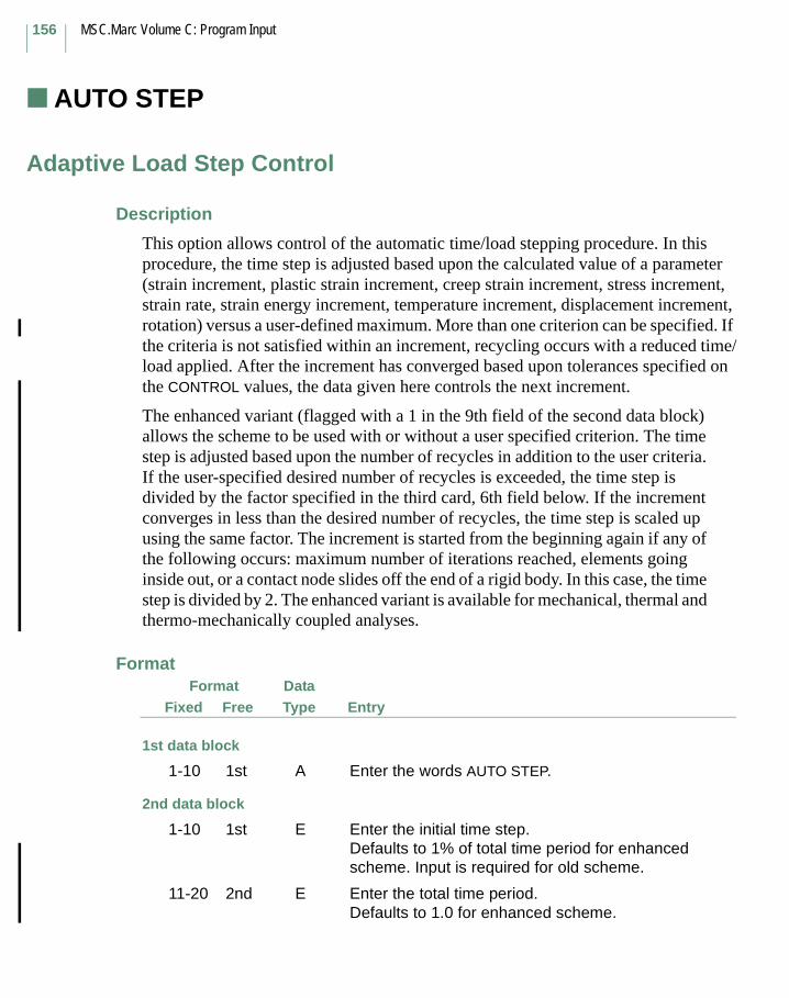
MSC.Marc Volume C: Program Input
156
AUTO STEP
Adaptive Load Step Control
Description
This option allows control of the automatic time/load stepping procedure. In this procedure, the time step is adjusted based upon the calculated value of a parameter (strain increment, plastic strain increment, creep strain increment, stress increment, strain rate, strain energy increment, temperature increment, displacement increment, rotation) versus a user-defined maximum. More than one criterion can be specified. If the criteria is not satisfied within an increment, recycling occurs with a reduced time/load applied. After the increment has converged based upon tolerances specified on the CONTROL values, the data given here controls the next increment.
The enhanced variant (flagged with a 1 in the 9th field of the second data block) allows the scheme to be used with or without a user specified criterion. The time step is adjusted based upon the number of recycles in addition to the user criteria. If the user-specified desired number of recycles is exceeded, the time step is divided by the factor specified in the third card, 6th field below. If the increment converges in less than the desired number of recycles, the time step is scaled up using the same factor. The increment is started from the beginning again if any of the following occurs: maximum number of iterations reached, elements going inside out, or a contact node slides off the end of a rigid body. In this case, the time step is divided by 2. The enhanced variant is available for mechanical, thermal and thermo-mechanically coupled analyses.
FormatFree Entry
DataTypeFixed
Format
1st data block
1-10 1st A Enter the words AUTO STEP.
2nd data block
1-10 1st E Enter the initial time step.Defaults to 1% of total time period for enhanced scheme. Input is required for old scheme.
11-20 2nd E Enter the total time period.Defaults to 1.0 for enhanced scheme.
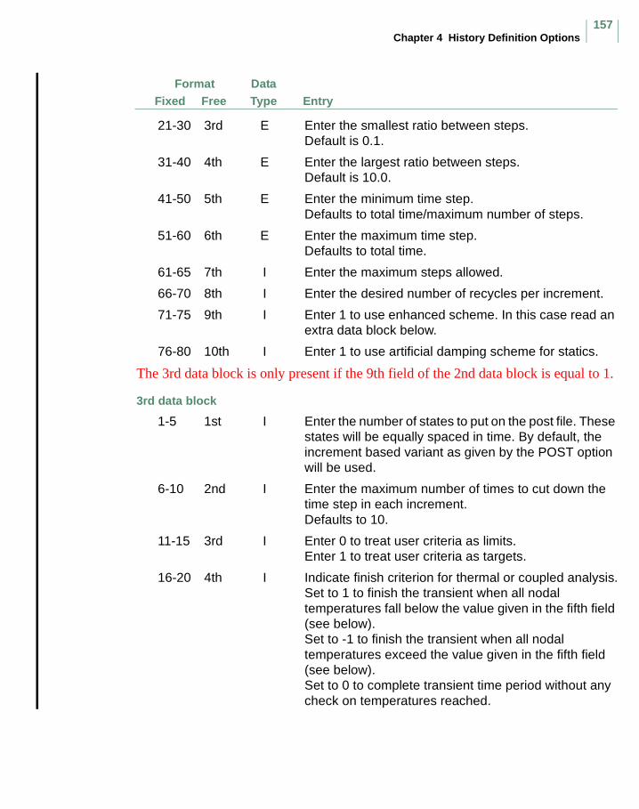
Chapter 4 History Definition Options157
FormatFree Entry
DataTypeFixed
21-30 3rd E Enter the smallest ratio between steps.Default is 0.1.
31-40 4th E Enter the largest ratio between steps.Default is 10.0.
41-50 5th E Enter the minimum time step.Defaults to total time/maximum number of steps.
51-60 6th E Enter the maximum time step.Defaults to total time.
61-65 7th I Enter the maximum steps allowed.
66-70 8th I Enter the desired number of recycles per increment.
71-75 9th I Enter 1 to use enhanced scheme. In this case read an extra data block below.
76-80 10th I Enter 1 to use artificial damping scheme for statics.
The 3rd data block is only present if the 9th field of the 2nd data block is equal to 1.
3rd data block
1-5 1st I Enter the number of states to put on the post file. These states will be equally spaced in time. By default, the increment based variant as given by the POST option will be used.
6-10 2nd I Enter the maximum number of times to cut down the time step in each increment.Defaults to 10.
11-15 3rd I Enter 0 to treat user criteria as limits.Enter 1 to treat user criteria as targets.
16-20 4th I Indicate finish criterion for thermal or coupled analysis.Set to 1 to finish the transient when all nodal temperatures fall below the value given in the fifth field (see below). Set to -1 to finish the transient when all nodal temperatures exceed the value given in the fifth field (see below). Set to 0 to complete transient time period without any check on temperatures reached.
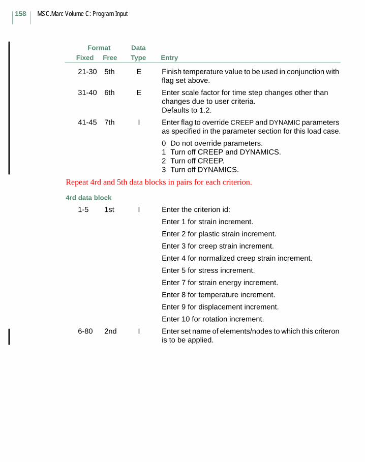
MSC.Marc Volume C: Program Input
158
FormatFree Entry
DataTypeFixed
21-30 5th E Finish temperature value to be used in conjunction with flag set above.
31-40 6th E Enter scale factor for time step changes other than changes due to user criteria.Defaults to 1.2.
41-45 7th I Enter flag to override CREEP and DYNAMIC parameters as specified in the parameter section for this load case.
0 Do not override parameters.1 Turn off CREEP and DYNAMICS.2 Turn off CREEP.3 Turn off DYNAMICS.
Repeat 4rd and 5th data blocks in pairs for each criterion.
4rd data block
1-5 1st I Enter the criterion id:
Enter 1 for strain increment.
Enter 2 for plastic strain increment.
Enter 3 for creep strain increment.
Enter 4 for normalized creep strain increment.
Enter 5 for stress increment.
Enter 7 for strain energy increment.
Enter 8 for temperature increment.
Enter 9 for displacement increment.
Enter 10 for rotation increment.
6-80 2nd I Enter set name of elements/nodes to which this criteron is to be applied.
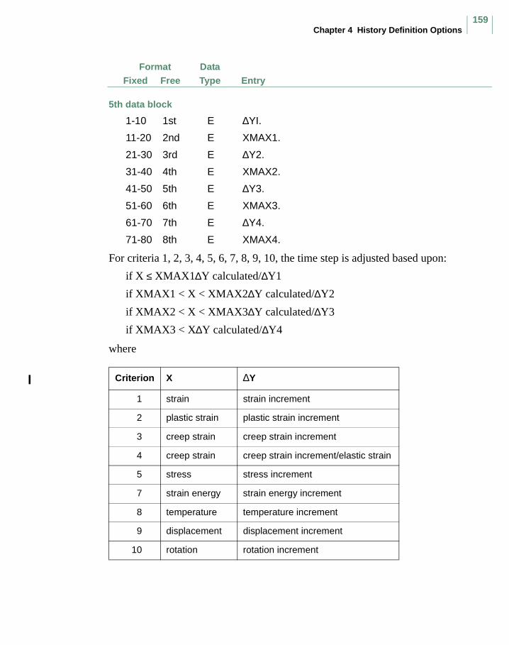
Chapter 4 History Definition Options159
FormatFree Entry
DataTypeFixed
5th data block
1-10 1st E ∆YI.
11-20 2nd E XMAX1.
21-30 3rd E ∆Y2.
31-40 4th E XMAX2.
41-50 5th E ∆Y3.
51-60 6th E XMAX3.
61-70 7th E ∆Y4.
71-80 8th E XMAX4.
For criteria 1, 2, 3, 4, 5, 6, 7, 8, 9, 10, the time step is adjusted based upon:
if X ≤ XMAX1∆Y calculated/∆Y1
if XMAX1 < X < XMAX2∆Y calculated/∆Y2
if XMAX2 < X < XMAX3∆Y calculated/∆Y3
if XMAX3 < X∆Y calculated/∆Y4
where
Criterion X ∆Y
1 strain strain increment
2 plastic strain plastic strain increment
3 creep strain creep strain increment
4 creep strain creep strain increment/elastic strain
5 stress stress increment
7 strain energy strain energy increment
8 temperature temperature increment
9 displacement displacement increment
10 rotation rotation increment

MSC.Marc Volume C: Program Input
160
CHANGE STATE (Model Definition)
Redefine State Variables
Description
This option provides various ways of changing the state variables throughout the model. State variables are initialized in the INITIAL STATE model definition set. The number of state variables per point is defined in the STATE VARS parameter. The default is one, with temperature always being the first state variable at a point. If more than one state variable per point has been assigned, this option can be used repeatedly to change the values of all state variables. The default value is no change if this option is not used. In this option, the values of the state variable at the end of the current increment are read in. When the temperature is being defined, the following points should be noted:
• For “history following analysis”, the thermal strains are based on temperature change during this step.
• For elastic re-analysis (ELASTIC parameter) the thermal strains are always based on temperature change between the initial, stress free temperature field and the values read in here.
• The AUTO LOAD option is available for specifying a time-varying history of state variables. The value of the total state variable at the end of each increment is specified.
• The AUTO THERM option is available for automatic control of a nonlinear (elastic-plastic) temperature loaded stress problem, to be used in conjunction with this option.
• The THERMAL LOADS option can be used as an alternate to input the change of temperature. Either incremental or total temperatures can be specified using this option.
• The AUTO THERM CREEP option is available for automatic control of a thermally loaded elastic-plastic-creep problem, to be used in conjunction with this option.
Four ways of changing any state variable through CHANGE STATE are possible:
• Read a range of elements, integration points and layers and a corresponding state variable value for the end of the current step.
• Read the state variable values for the end of the current step through user subroutine NEWSV.

Chapter 4 History Definition Options161
• Read the state variable values for the end of the current step from a named step of the post file output from a previous heat transfer analysis with Marc. With this option, Marc assumes direct correspondence of the post file elements with the elements in the current analysis. Any spatial interpolation must be provided separately by the user. For AUTO LOAD, a one-to-one correspondence between the thermal increments on the post file and the mechanical increments is assumed between the user-defined starting and ending post increments. For AUTO THERM or AUTO THERM CREEP, based on the user-defined allowable temperature change, the thermal increments on the post file can be subdivided into many mechanical increments. Providing state variables through the thermal post file is not currently supported for other adaptive stepping procedures.
• Read a list of elements, integration points, and layers and a corresponding state variable value.
It should be noted that the end of the current step is interpreted as the end of the current increment for fixed stepping procedures (AUTO LOAD, DYNAMIC CHANGE, CREEP INCREMENT) and as the end of the loadcase for adaptive stepping procedures (AUTO STEP, AUTO THERM, AUTO TIME, AUTO INCREMENT, AUTO CREEP).
Note: Using this option, total state variable values are input. From MSC.Marc 2001 onwards, the incremental change in the state variables is reset to 0 bevore each new increment for AUTO LOAD.
FormatFree Entry
DataTypeFixed
Format
1st data block
1-12 1st A Enter the words CHANGE STATE.
2nd data block
1-5 1st I Enter the state variable identifier for the state variable being changed (1,2,3,etc.) 1 = temperature. If more than one state variable is being used, the STATE VARS parameter must be included.

MSC.Marc Volume C: Program Input
162
FormatFree Entry
DataTypeFixed
6-10 2nd I Enter 1 to change the state variable via the 3rd and 4th data blocks below. In this case, the third field must also be defined.
Enter 2 to change the state variable via user subroutine NEWSV. This subroutine is now called in a loop on all the elements in the mesh.
Enter 3 to read the new values of the state variable from a post file written by a previous heat transfer analysis. In this case, the fourth and fifth field must be defined.
Enter 4 to change the state variable via data blocks 5, 6, 7, and 8 below.
11-15 3rd I Only nonzero if the second field is set to 1 or 4. In that case, this entry gives the number of data blocks set in data blocks 3 and 4 used to input the new value of the state variable (optional).
16-20 4th I Only nonzero if the second field is set to 3. Then. this entry defines the unit number from which the post file information from the previous heat transfer run is read. Defaults to unit 24 for a formatted post file, and to unit 25 for a binary post file.
21-25 5th I Only nonzero if the second field is set to 3. In that case, this entry defines the step number on the heat transfer run post file to be read as the definition of the new value of the state variable at the end of the current step. This is currently only supported for AUTO LOAD and AUTO THERM.
26-30 6th I Only used if the AUTO LOAD or AUTO THERM options are in use. Give the number of sets of input to be read to define the temperature history.
31-35 7th I Enter 1 if formatted post file is used.
For Cray Only:
Set to 2 for IEEE binary file.
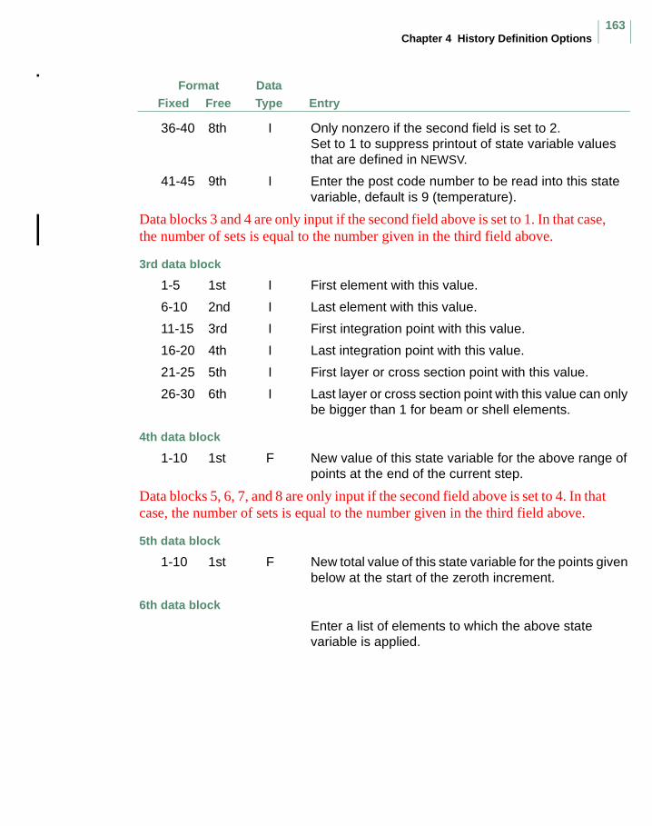
Chapter 4 History Definition Options163
FormatFree Entry
DataTypeFixed
36-40 8th I Only nonzero if the second field is set to 2. Set to 1 to suppress printout of state variable values that are defined in NEWSV.
41-45 9th I Enter the post code number to be read into this state variable, default is 9 (temperature).
Data blocks 3 and 4 are only input if the second field above is set to 1. In that case, the number of sets is equal to the number given in the third field above.
3rd data block
1-5 1st I First element with this value.
6-10 2nd I Last element with this value.
11-15 3rd I First integration point with this value.
16-20 4th I Last integration point with this value.
21-25 5th I First layer or cross section point with this value.
26-30 6th I Last layer or cross section point with this value can only be bigger than 1 for beam or shell elements.
4th data block
1-10 1st F New value of this state variable for the above range of points at the end of the current step.
Data blocks 5, 6, 7, and 8 are only input if the second field above is set to 4. In that case, the number of sets is equal to the number given in the third field above.
5th data block
1-10 1st F New total value of this state variable for the points given below at the start of the zeroth increment.
6th data block
Enter a list of elements to which the above state variable is applied.

MSC.Marc Volume C: Program Input
164
FormatFree Entry
DataTypeFixed
7th data block
This data block is not necessary if the CENTROID parameter is used.
Enter a list of integration points to which the above state variable is applied.
8th data block
This data block is only necessary if there are either beams or shells in the mesh.
Enter a list of layer points to which the above state variable is applied.

Chapter 4 History Definition Options165
POINT TEMP (History Definition)
Define Point Temperatures
Description
This option defines temperatures at nodal points for an uncoupled thermal stress problems at the end of the increment.
Note: For shell analyses, a uniform temperature is used through the thickness direction.
FormatFree Entry
DataTypeFixed
Format
1st data block
1-10 1st A Enter the words POINT TEMP.
2nd data block
1-5 1st I Enter the number of sets of prescribed temperatures (optional).Enter -1 if USINC user subtroutine is used. In this case, the 3rd and 4th data blocks are not used.
6-10 2nd I Enter file number for input of prescribed temperatures data.Defaults to input.
11-15 3rd I Flag to indicate that temperatures are read from previously generated post file. Set to 1.
16-20 4th I Only nonzero if the third field is set to 1. This entry defines the unit number from which the post file information is read.
21-25 5th I Enter step number to be read.
26-30 6th I Enter 1 if a formatted post file is used.
For Cray Only:
Set to 2 for IEEE binary file.

MSC.Marc Volume C: Program Input
166
FormatFree Entry
DataTypeFixed
Data blocks 3 and 4 are given in NSET pairs, only if the flag in the third field is not equal to 1.
3rd data block
1-10 1st E Temperatures at the end of the increment.
4th data block
Enter list of nodes for which the above initial temperature is applied.
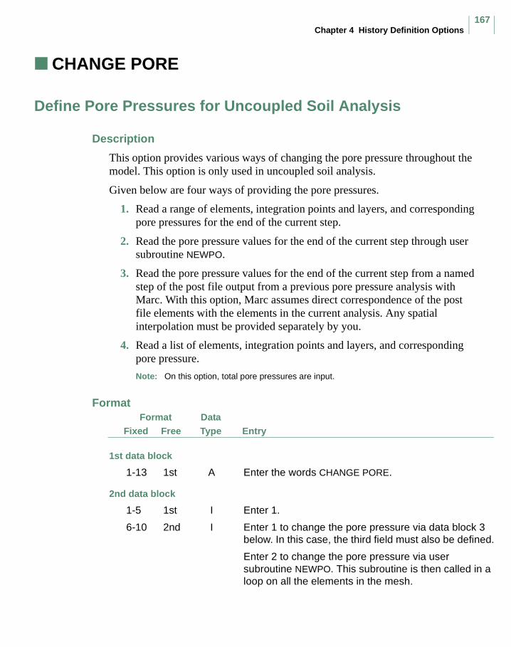
Chapter 4 History Definition Options167
CHANGE PORE (History Definition)
Define Pore Pressures for Uncoupled Soil Analysis
Description
This option provides various ways of changing the pore pressure throughout the model. This option is only used in uncoupled soil analysis.
Given below are four ways of providing the pore pressures.
1. Read a range of elements, integration points and layers, and corresponding pore pressures for the end of the current step.
2. Read the pore pressure values for the end of the current step through user subroutine NEWPO.
3. Read the pore pressure values for the end of the current step from a named step of the post file output from a previous pore pressure analysis with Marc. With this option, Marc assumes direct correspondence of the post file elements with the elements in the current analysis. Any spatial interpolation must be provided separately by you.
4. Read a list of elements, integration points and layers, and corresponding pore pressure.
Note: On this option, total pore pressures are input.
FormatFree Entry
DataTypeFixed
Format
1st data block
1-13 1st A Enter the words CHANGE PORE.
2nd data block
1-5 1st I Enter 1.
6-10 2nd I Enter 1 to change the pore pressure via data block 3 below. In this case, the third field must also be defined.
Enter 2 to change the pore pressure via user subroutine NEWPO. This subroutine is then called in a loop on all the elements in the mesh.
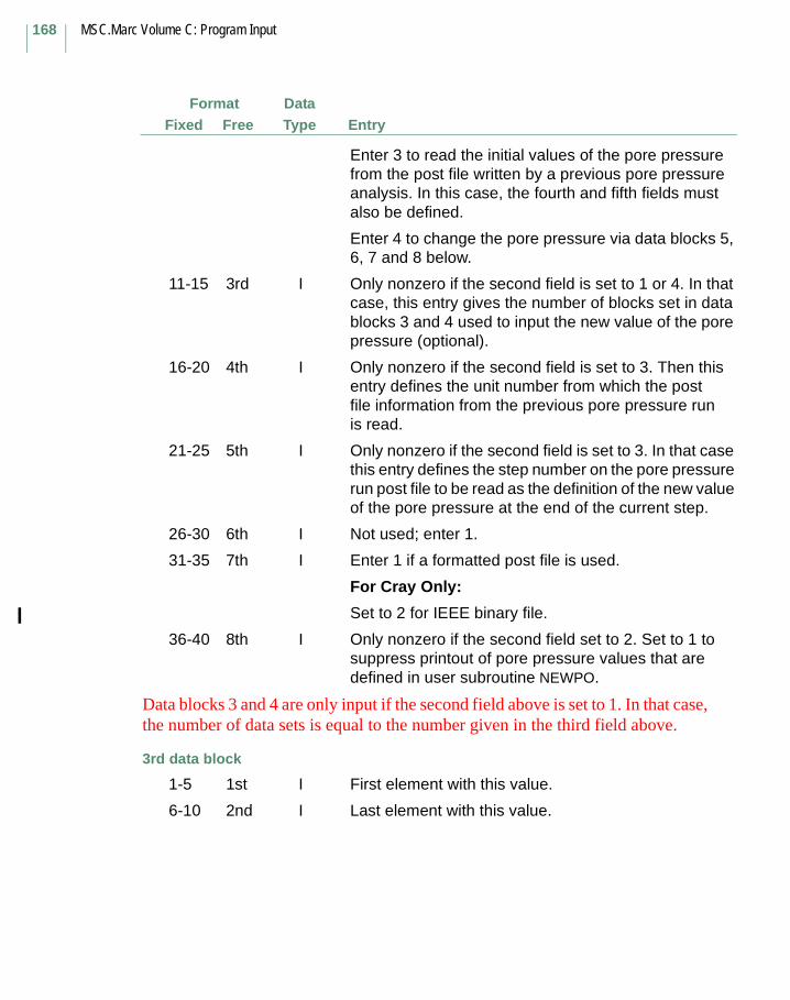
MSC.Marc Volume C: Program Input
168
FormatFree Entry
DataTypeFixed
Enter 3 to read the initial values of the pore pressure from the post file written by a previous pore pressure analysis. In this case, the fourth and fifth fields must also be defined.
Enter 4 to change the pore pressure via data blocks 5, 6, 7 and 8 below.
11-15 3rd I Only nonzero if the second field is set to 1 or 4. In that case, this entry gives the number of blocks set in data blocks 3 and 4 used to input the new value of the pore pressure (optional).
16-20 4th I Only nonzero if the second field is set to 3. Then this entry defines the unit number from which the post file information from the previous pore pressure run is read.
21-25 5th I Only nonzero if the second field is set to 3. In that case this entry defines the step number on the pore pressure run post file to be read as the definition of the new value of the pore pressure at the end of the current step.
26-30 6th I Not used; enter 1.
31-35 7th I Enter 1 if a formatted post file is used.
For Cray Only:
Set to 2 for IEEE binary file.
36-40 8th I Only nonzero if the second field set to 2. Set to 1 to suppress printout of pore pressure values that are defined in user subroutine NEWPO.
Data blocks 3 and 4 are only input if the second field above is set to 1. In that case, the number of data sets is equal to the number given in the third field above.
3rd data block
1-5 1st I First element with this value.
6-10 2nd I Last element with this value.
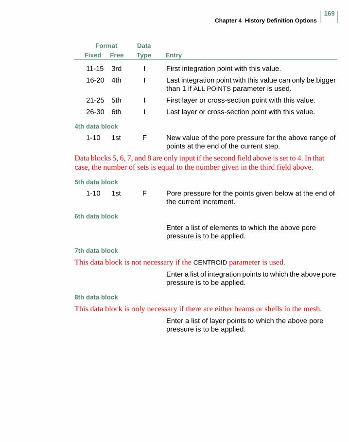
Chapter 4 History Definition Options169
FormatFree Entry
DataTypeFixed
11-15 3rd I First integration point with this value.
16-20 4th I Last integration point with this value can only be bigger than 1 if ALL POINTS parameter is used.
21-25 5th I First layer or cross-section point with this value.
26-30 6th I Last layer or cross-section point with this value.
4th data block
1-10 1st F New value of the pore pressure for the above range of points at the end of the current step.
Data blocks 5, 6, 7, and 8 are only input if the second field above is set to 4. In that case, the number of sets is equal to the number given in the third field above.
5th data block
1-10 1st F Pore pressure for the points given below at the end of the current increment.
6th data block
Enter a list of elements to which the above pore pressure is to be applied.
7th data block
This data block is not necessary if the CENTROID parameter is used.
Enter a list of integration points to which the above pore pressure is to be applied.
8th data block
This data block is only necessary if there are either beams or shells in the mesh.
Enter a list of layer points to which the above pore pressure is to be applied.
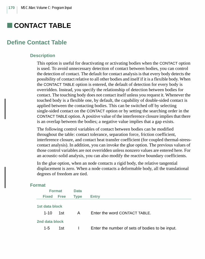
MSC.Marc Volume C: Program Input
170
CONTACT TABLE (History Definition)
Define Contact Table
Description
This option is useful for deactivating or activating bodies when the CONTACT option is used. To avoid unnecessary detection of contact between bodies, you can control the detection of contact. The default for contact analysis is that every body detects the possibility of contact relative to all other bodies and itself if it is a flexible body. When the CONTACT TABLE option is entered, the default of detection for every body is overridden. Instead, you specify the relationship of detection between bodies for contact. The touching body does not contact itself unless you request it. Whenever the touched body is a flexible one, by default, the capability of double-sided contact is applied between the contacting bodies. This can be switched off by selecting single-sided contact on the CONTACT option or by setting the searching order in the CONTACT TABLE option. A positive value of the interference closure implies that there is an overlap between the bodies; a negative value implies that a gap exists.
The following control variables of contact between bodies can be modified throughout the table: contact tolerance, separation force, friction coefficient, interference closure, and contact heat transfer coefficient (for coupled thermal-stress-contact analysis). In addition, you can invoke the glue option. The previous values of those control variables are not overridden unless nonzero values are entered here. For an acoustic-solid analysis, you can also modify the reactive boundary coefficients.
In the glue option, when an node contacts a rigid body, the relative tangential displacement is zero. When a node contacts a deformable body, all the translational degrees of freedom are tied.
FormatFree Entry
DataTypeFixed
Format
1st data block
1-10 1st A Enter the word CONTACT TABLE.
2nd data block
1-5 1st I Enter the number of sets of bodies to be input.
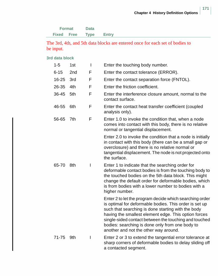
Chapter 4 History Definition Options171
FormatFree Entry
DataTypeFixed
The 3rd, 4th, and 5th data blocks are entered once for each set of bodies to be input.
3rd data block
1-5 1st I Enter the touching body number.
6-15 2nd F Enter the contact tolerance (ERROR).
16-25 3rd F Enter the contact separation force (FNTOL).
26-35 4th F Enter the friction coefficient.
36-45 5th F Enter the interference closure amount, normal to the contact surface.
46-55 6th F Enter the contact heat transfer coefficient (coupled analysis only).
56-65 7th F Enter 1.0 to invoke the condition that, when a node comes into contact with this body, there is no relative normal or tangential displacement.
Enter 2.0 to invoke the condition that a node is initially in contact with this body (there can be a small gap or overclosure) and there is no relative normal or tangential displacement. The node is not projected onto the surface.
65-70 8th I Enter 1 to indicate that the searching order for deformable contact bodies is from the touching body to the touched bodies on the 5th data block. This might change the default order for deformable bodies, which is from bodies with a lower number to bodies with a higher number.
Enter 2 to let the program decide which searching order is optimal for deformable bodies. This order is set up such that searching is done starting with the body having the smallest element edge. This option forces single-sided contact between the touching and touched bodies: searching is done only from one body to another and not the other way around.
71-75 9th I Enter 2 or 3 to extend the tangential error tolerance at sharp corners of deformable bodies to delay sliding off a contacted segment.
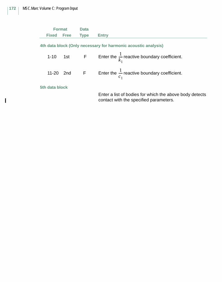
MSC.Marc Volume C: Program Input
172
FormatFree Entry
DataTypeFixed
4th data block (Only necessary for harmonic acoustic analysis)
1-10 1st F Enter the reactive boundary coefficient.
11-20 2nd F Enter the reactive boundary coefficient.
5th data block
Enter a list of bodies for which the above body detects contact with the specified parameters.
1k1-----
1c1-----

Chapter 5 Rezoning Options173
Chapter 5 Rezoning Options
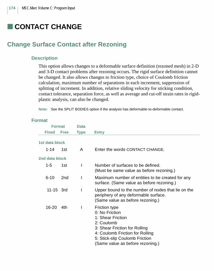
MSC.Marc Volume C: Program Input
174
CONTACT CHANGE
Change Surface Contact after Rezoning
Description
This option allows changes to a deformable surface definition (rezoned mesh) in 2-D and 3-D contact problems after rezoning occurs. The rigid surface definition cannot be changed. It also allows changes to friction type, choice of Coulomb friction calculation, maximum number of separations in each increment, suppression of splitting of increment. In addition, relative sliding velocity for sticking condition, contact tolerance, separation force, as well as average and cut-off strain rates in rigid-plastic analysis, can also be changed.
Note: See the SPLIT BODIES option if the analysis has deformable-to-deformable contact.
FormatFree Entry
DataTypeFixed
Format
1st data block
1-14 1st A Enter the words CONTACT CHANGE.
2nd data block
1-5 1st I Number of surfaces to be defined.(Must be same value as before rezoning.)
6-10 2nd I Maximum number of entities to be created for any surface. (Same value as before rezoning.)
11-15 3rd I Upper bound to the number of nodes that lie on the periphery of any deformable surface. (Same value as before rezoning.)
16-20 4th I Friction type0: No Friction 1: Shear Friction 2: Coulomb3: Shear Friction for Rolling4: Coulomb Friction for Rolling5: Stick-slip Coulomb Friction(Same value as before rezoning.)
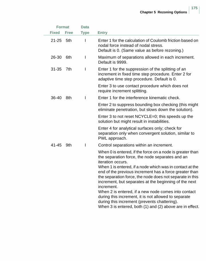
Chapter 5 Rezoning Options175
FormatFree Entry
DataTypeFixed
21-25 5th I Enter 1 for the calculation of Coulomb friction based on nodal force instead of nodal stress. Default is 0. (Same value as before rezoning.)
26-30 6th I Maximum of separations allowed in each increment. Default is 9999.
31-35 7th I Enter 1 for the suppression of the splitting of an increment in fixed time step procedure. Enter 2 for adaptive time step procedure. Default is 0.
Enter 3 to use contact procedure which does not require increment splitting.
36-40 8th I Enter 1 for the interference kinematic check.
Enter 2 to suppress bounding box checking (this might eliminate penetration, but slows down the solution).
Enter 3 to not reset NCYCLE=0; this speeds up the solution but might result in instabilities.
Enter 4 for analytical surfaces only; check for separation only when convergent solution, similar to PWL approach.
41-45 9th I Control separations within an increment.
When 0 is entered, if the force on a node is greater than the separation force, the node separates and an iteration occurs.When 1 is entered, if a node which was in contact at the end of the previous increment has a force greater than the separation force, the node does not separate in this increment, but separates at the beginning of the next increment.When 2 is entered, if a new node comes into contact during this increment, it is not allowed to separate during this increment (prevents chattering).When 3 is entered, both (1) and (2) above are in effect.
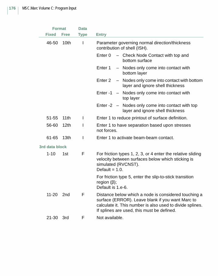
MSC.Marc Volume C: Program Input
176
FormatFree Entry
DataTypeFixed
46-50 10th I Parameter governing normal direction/thickness contribution of shell (ISH).
Enter 0 – Check Node Contact with top and bottom surface
Enter 1 – Nodes only come into contact with bottom layer
Enter 2 – Nodes only come into contact with bottom layer and ignore shell thickness
Enter -1 – Nodes only come into contact with top layer
Enter -2 – Nodes only come into contact with top layer and ignore shell thickness
51-55 11th I Enter 1 to reduce printout of surface definition.
56-60 12th I Enter 1 to have separation based upon stresses not forces.
61-65 13th I Enter 1 to activate beam-beam contact.
3rd data block
1-10 1st F For friction types 1, 2, 3, or 4 enter the relative sliding velocity between surfaces below which sticking is simulated (RVCNST).Default = 1.0.
For friction type 5, enter the slip-to-stick transition region (β);Default is 1.e-6.
11-20 2nd F Distance below which a node is considered touching a surface (ERROR). Leave blank if you want Marc to calculate it. This number is also used to divide splines. If splines are used, this must be defined.
21-30 3rd F Not available.
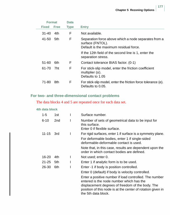
Chapter 5 Rezoning Options177
FormatFree Entry
DataTypeFixed
31-40 4th F Not available.
41-50 5th F Separation force above which a node separates from a surface (FNTOL).Default is the maximum residual force.
If the 12th field of the second line is 1, enter the separation stress.
51-60 6th F Contact tolerance BIAS factor. (0-1)
61-70 7ht F For stick-slip model, enter the friction coefficient multiplier (α).Defaults to 1.05
71-80 8th F For stick-slip model, enter the friction force tolerance (e).Defaults to 0.05.
For two- and three-dimensional contact problems
The data blocks 4 and 5 are repeated once for each data set.
4th data block
1-5 1st I Surface number.
6-10 2nd I Number of sets of geometrical data to be input for this surface. Enter 0 if flexible surface.
11-15 3rd I For rigid surfaces, enter 1 if surface is a symmetry plane.
For deformable bodies, enter 1 if single-sided deformable-deformable contact is used.
Note that, in this case, results are dependent upon the order in which contact bodies are defined.
16-20 4th I Not used; enter 0.
21-25 5th I Enter 1 if analytic form is to be used.
26-30 6th I Enter -1 if body is position controlled.
Enter 0 (default) if body is velocity controlled.
Enter a positive number if load controlled. The number entered is the node number which has the displacement degrees of freedom of the body. The position of this node is at the center of rotation given in the 5th data block.

MSC.Marc Volume C: Program Input
178
FormatFree Entry
DataTypeFixed
31-35 7th I Enter a positive number if load controlled and rotations are allowed. The number is the node number which has the rotation(s) of the body as degrees of freedom. The position of this node is at the center of rotation given in the 5th data block.
36-40 8th I Contact body type (optional):
1: rigid body;2: deformable body;3: symmetry body;4: heat-rigid body;5: workpiece;6: acoustic body.
41-64 9th A Contact body name (optional)
The 5th data block is only necessary if the surface is deformable; if the surface is rigid, no additional data is required.
5th data block
Enter a list of elements of which the surface is comprised.

Appendix A Program Messages179
Appendix A Program Messages
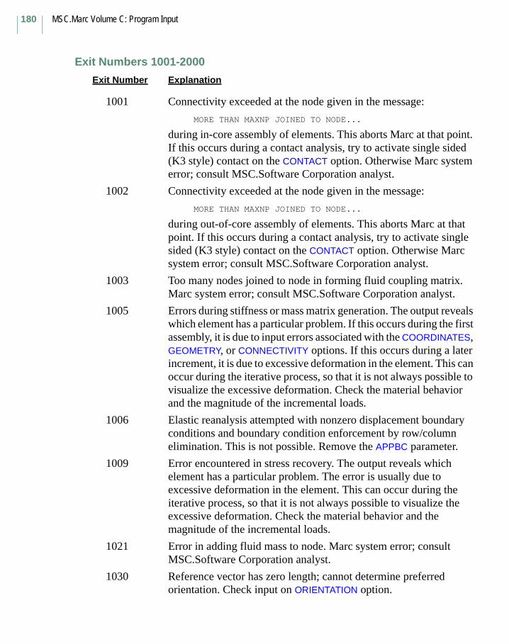
MSC.Marc Volume C: Program Input
180
Exit Numbers 1001-2000
Exit Number Explanation
1001 Connectivity exceeded at the node given in the message:
MORE THAN MAXNP JOINED TO NODE...
during in-core assembly of elements. This aborts Marc at that point. If this occurs during a contact analysis, try to activate single sided (K3 style) contact on the CONTACT option. Otherwise Marc system error; consult MSC.Software Corporation analyst.
1002 Connectivity exceeded at the node given in the message:
MORE THAN MAXNP JOINED TO NODE...
during out-of-core assembly of elements. This aborts Marc at that point. If this occurs during a contact analysis, try to activate single sided (K3 style) contact on the CONTACT option. Otherwise Marc system error; consult MSC.Software Corporation analyst.
1003 Too many nodes joined to node in forming fluid coupling matrix. Marc system error; consult MSC.Software Corporation analyst.
1005 Errors during stiffness or mass matrix generation. The output reveals which element has a particular problem. If this occurs during the first assembly, it is due to input errors associated with the COORDINATES, GEOMETRY, or CONNECTIVITY options. If this occurs during a later increment, it is due to excessive deformation in the element. This can occur during the iterative process, so that it is not always possible to visualize the excessive deformation. Check the material behavior and the magnitude of the incremental loads.
1006 Elastic reanalysis attempted with nonzero displacement boundary conditions and boundary condition enforcement by row/column elimination. This is not possible. Remove the APPBC parameter.
1009 Error encountered in stress recovery. The output reveals which element has a particular problem. The error is usually due to excessive deformation in the element. This can occur during the iterative process, so that it is not always possible to visualize the excessive deformation. Check the material behavior and the magnitude of the incremental loads.
1021 Error in adding fluid mass to node. Marc system error; consult MSC.Software Corporation analyst.
1030 Reference vector has zero length; cannot determine preferred orientation. Check input on ORIENTATION option.
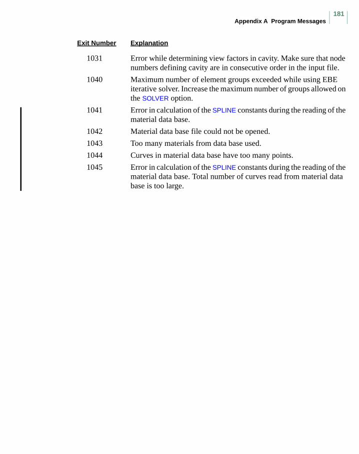
Appendix A Program Messages181
Exit Number Explanation
1031 Error while determining view factors in cavity. Make sure that node numbers defining cavity are in consecutive order in the input file.
1040 Maximum number of element groups exceeded while using EBE iterative solver. Increase the maximum number of groups allowed on the SOLVER option.
1041 Error in calculation of the SPLINE constants during the reading of the material data base.
1042 Material data base file could not be opened.
1043 Too many materials from data base used.
1044 Curves in material data base have too many points.
1045 Error in calculation of the SPLINE constants during the reading of the material data base. Total number of curves read from material data base is too large.

MSC.Marc Volume C: Program Input
182
Appendix B Workspace Definition and the Sizing Option
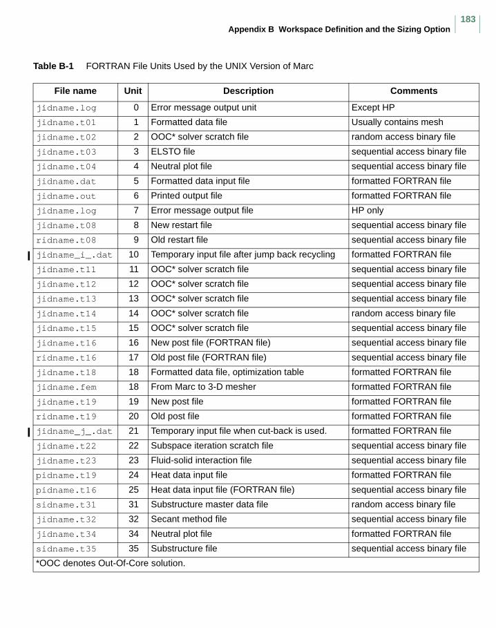
Appendix B Workspace Definition and the Sizing Option183
Table B-1 FORTRAN File Units Used by the UNIX Version of Marc
File name Unit Description Comments
jidname.log 0 Error message output unit Except HP
jidname.t01 1 Formatted data file Usually contains mesh
jidname.t02 2 OOC* solver scratch file random access binary file
jidname.t03 3 ELSTO file sequential access binary file
jidname.t04 4 Neutral plot file sequential access binary file
jidname.dat 5 Formatted data input file formatted FORTRAN file
jidname.out 6 Printed output file formatted FORTRAN file
jidname.log 7 Error message output file HP only
jidname.t08 8 New restart file sequential access binary file
ridname.t08 9 Old restart file sequential access binary file
jidname_i_.dat 10 Temporary input file after jump back recycling formatted FORTRAN file
jidname.t11 11 OOC* solver scratch file sequential access binary file
jidname.t12 12 OOC* solver scratch file sequential access binary file
jidname.t13 13 OOC* solver scratch file sequential access binary file
jidname.t14 14 OOC* solver scratch file random access binary file
jidname.t15 15 OOC* solver scratch file sequential access binary file
jidname.t16 16 New post file (FORTRAN file) sequential access binary file
ridname.t16 17 Old post file (FORTRAN file) sequential access binary file
jidname.t18 18 Formatted data file, optimization table formatted FORTRAN file
jidname.fem 18 From Marc to 3-D mesher formatted FORTRAN file
jidname.t19 19 New post file formatted FORTRAN file
ridname.t19 20 Old post file formatted FORTRAN file
jidname_j_.dat 21 Temporary input file when cut-back is used. formatted FORTRAN file
jidname.t22 22 Subspace iteration scratch file sequential access binary file
jidname.t23 23 Fluid-solid interaction file sequential access binary file
pidname.t19 24 Heat data input file formatted FORTRAN file
pidname.t16 25 Heat data input file (FORTRAN file) sequential access binary file
sidname.t31 31 Substructure master data file random access binary file
jidname.t32 32 Secant method file sequential access binary file
jidname.t34 34 Neutral plot file formatted FORTRAN file
sidname.t35 35 Substructure file sequential access binary file
*OOC denotes Out-Of-Core solution.

MSC.Marc Volume C: Program Input
184
sidname.t36 36 Substructure file sequential access binary file
jidname.t41 41 New Post file – Domain Decomposition sequential access binary
ridname.t42 42 Post file – Domain Decomposition formatted FORTRAN file
jidname.t45 45 Optimization data file formatted FORTRAN file
jidname.t46 46 Optimization scratch file formatted FORTRAN file
jidname.trk 47 New particle tracking file formatted FORTRAN file
ridname.trk 48 Old particle tracking file formatted FORTRAN file
jidname.cntl 52 Dynamic control file formatted FORTRAN file
jidname.seq 53 Sequence option formatted FORTRAN file
jidname.rst 54 Load case data formatted FORTRAN file
jidname.mesh 55 User supplied mesh formatted FORTRAN file
jidname.feb 55 From 3-D mesher to Marc formatted FORTRAN file
jidname.pass 56 Auto restart command line formatted FORTRAN file
jidname.rms 57 2D outline file for remeshing formatted FORTRAN file
jidname.domeshjidname.donemesh
59 Lock files indicating meshing status formatted FORTRAN file
jidname.sts 67 Analysis progress reporting file formatted FORTRAN file
USRDEF 98 Global default file formatted FORTRAN file
EXITMSG 99 Exit messages formatted FORTRAN file
Table B-1 FORTRAN File Units Used by the UNIX Version of Marc (Continued)
File name Unit Description Comments
*OOC denotes Out-Of-Core solution.

Appendix F Material Database185
Appendix F Material Database

MSC.Marc Volume C: Program Input
186
To enter a new material into the database, the following steps would be performed.
Please use the name convention followed in Marc to be certain that Marc reads your material data file properly. Using the convention, Marc will exit with error if the file with the material name does not exist in the directory. The user-defined material data should use the prefix of usr_ and the file extension for the flow stress data should be .mat. Eight characters are allowed after usr_. For example, if you name your material as usr_material, you will create one use_material.mud or use_material.mfd file for Mentat database and one flow stress data file, usr_material.mat for the analysis. You have to place the Mentat database file in mentat/materials/directory. You can put the flow stress file in your current job directory or in marc/AF_flowmat directory if you want to share it with other users. Once you have done the preparation for the material database, you can use it in setting up your finite element model file in the future.
APPENDIX
F Material Database
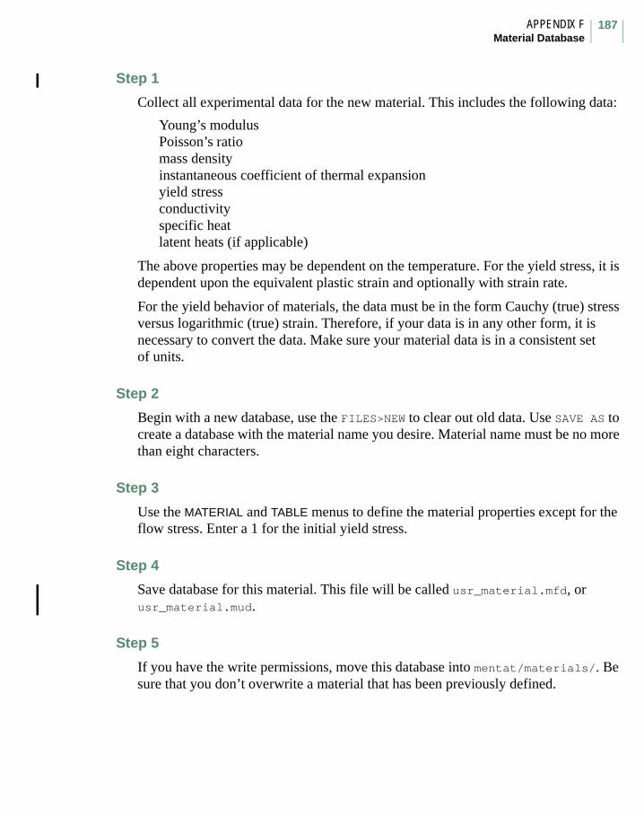
APPENDIX FMaterial Database
187
Step 1
Collect all experimental data for the new material. This includes the following data:
Young’s modulusPoisson’s ratiomass densityinstantaneous coefficient of thermal expansionyield stressconductivityspecific heatlatent heats (if applicable)
The above properties may be dependent on the temperature. For the yield stress, it is dependent upon the equivalent plastic strain and optionally with strain rate.
For the yield behavior of materials, the data must be in the form Cauchy (true) stress versus logarithmic (true) strain. Therefore, if your data is in any other form, it is necessary to convert the data. Make sure your material data is in a consistent set of units.
Step 2
Begin with a new database, use the FILES>NEW to clear out old data. Use SAVE AS to create a database with the material name you desire. Material name must be no more than eight characters.
Step 3
Use the MATERIAL and TABLE menus to define the material properties except for the flow stress. Enter a 1 for the initial yield stress.
Step 4
Save database for this material. This file will be called usr_material.mfd, or usr_material.mud.
Step 5
If you have the write permissions, move this database into mentat/materials/. Be sure that you don’t overwrite a material that has been previously defined.

MSC.Marc Volume C: Program Input
188
Step 6
Use the editor to define a file for the flow stress. This file should be called usr_material.dat.
The structure of this file is as follows:
Data structure in x_xxxxcc.dat
1. data card: Material name beginning in column one with thematerial identification number
Format : character*40Example : 3.2318 AlMgSi 1
2. data card: ncurves, npoints, ntemps, nerates, number of :where ncurves : number of curves in input (Max. 400)
npoints : number of data points in each curve (Max. 100)ntemps : number of reference temperatures (Max. 20)nerates : number of reference strain rates (Max. 20)
Format : four integer in free formatExample : 30, 13, 5, 6
3. data card: eqpemin, eqpemax, equivalent plastic strain range of thematerial described in this input eqpeminmust be = 0.0, logarithmic strain measure
Format : two real in free formatExample : 0.0, 7.0,
4. data card: eratmin, eratmax, equivalent plastic strain rate range of thematerial described in this input
Format : two real in free formatExample : 0.2, 10.0,
5. data card: eratmin, eratmax, Temperature range of the materialdescribed in this input
Format : two real in free formatExample : 350.0, 550.0,
The following data are repeated “ ncurves “ time (See card 2)
6. 0 data card : documentation text, character*80
6. 1 data card : icurve, temp., erate, sequential curve identification number, Temperature and equivalent plastic strain rate
6. 2 data card : eqpmin, eq_stress, logarithmic equivalent plastic strain and equivalent von mises (true) stress (first point)
6. n data card : eqpmax, eq_stress, logarithmic equivalent plastic strain and equivalent von mises (true) stress (npoint’th point, see card 2)

APPENDIX FMaterial Database
189
6.0 : Format : character*80Example : === CURVE_01 Sig_Yiel, T=350. C, Eps_dot=0.2 1/s
6.1 : Format : one integer, two real in free formatExample : 1, 350.0, 0.20,
6.2 : Format : two real in free formatExample : 0.00, 78.0,
6.i : Format : two real in free formatExample : 11.75, 59.0,0,
6.n : Format : two real in free formatExample : 7.00, 52.0,
•••
Step 7
Save file and move file into marc/AF_flowmat/.
Step 8
Your new material can now be read from:
material properties>Read>Read other materials.

MSC.Marc Volume C: Program Input
190

Volume D: User Subroutines and Special Routines1
Volume D: User Subroutines and
Special Routines

MSC.Marc Volume D: User Subroutines and Special Routines
2
Chapter 2 User-defined Loading Boundary Conditions and State Variables User Subroutines
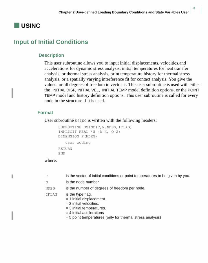
Chapter 2 User-defined Loading Boundary Conditions and State Variables User3
USINC
Input of Initial Conditions
Description
This user subroutine allows you to input initial displacements, velocities,and accelerations for dynamic stress analysis, initial temperatures for heat transfer analysis, or thermal stress analysis, print temperature history for thermal stress analysis, or a spatially varying interference fit for contact analysis. You give the values for all degrees of freedom in vector F. This user subroutine is used with either the INITIAL DISP, INITIAL VEL, INITIAL TEMP model definition options, or the POINT TEMP model and history definition options. This user subroutine is called for every node in the structure if it is used.
Format
User subroutine USINC is written with the following headers:SUBROUTINE USINC(F,N,NDEG,IFLAG)IMPLICIT REAL *8 (A-H, O-Z)DIMENSION F(NDEG)
user coding
RETURNEND
where:
F is the vector of initial conditions or point temperatures to be given by you.
N is the node number.
NDEG is the number of degrees of freedom per node.
IFLAG is the type flag.= 1 initial displacement.= 2 initial velocities.= 3 initial temperatures. = 4 initial acellerations= 5 point temperatures (only for thermal stress analysis)
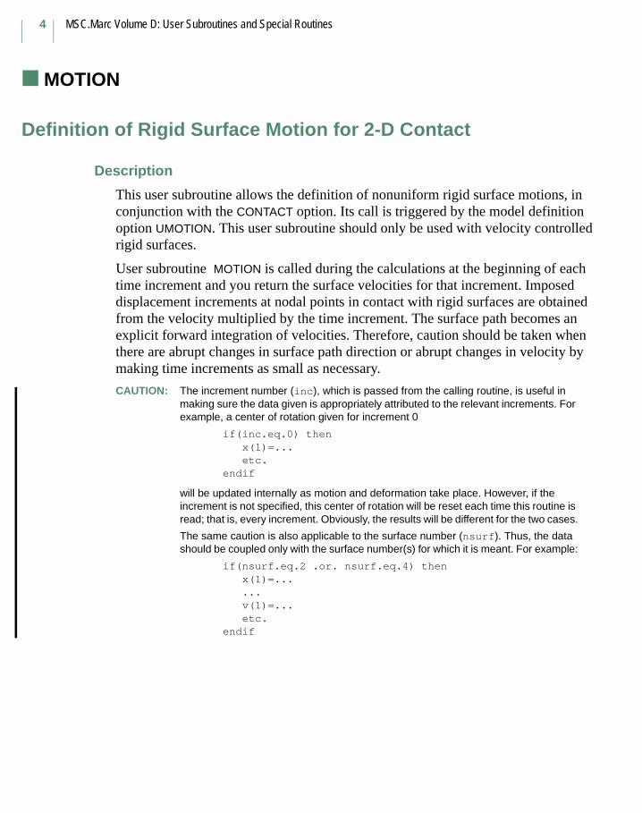
MSC.Marc Volume D: User Subroutines and Special Routines
4
MOTION (2-D)
Definition of Rigid Surface Motion for 2-D Contact
Description
This user subroutine allows the definition of nonuniform rigid surface motions, in conjunction with the CONTACT option. Its call is triggered by the model definition option UMOTION. This user subroutine should only be used with velocity controlled rigid surfaces.
User subroutine MOTION is called during the calculations at the beginning of each time increment and you return the surface velocities for that increment. Imposed displacement increments at nodal points in contact with rigid surfaces are obtained from the velocity multiplied by the time increment. The surface path becomes an explicit forward integration of velocities. Therefore, caution should be taken when there are abrupt changes in surface path direction or abrupt changes in velocity by making time increments as small as necessary.
CAUTION: The increment number (inc), which is passed from the calling routine, is useful in making sure the data given is appropriately attributed to the relevant increments. For example, a center of rotation given for increment 0
if(inc.eq.0) thenx(1)=...etc.
endif
will be updated internally as motion and deformation take place. However, if the increment is not specified, this center of rotation will be reset each time this routine is read; that is, every increment. Obviously, the results will be different for the two cases.
The same caution is also applicable to the surface number (nsurf). Thus, the data should be coupled only with the surface number(s) for which it is meant. For example:
if(nsurf.eq.2 .or. nsurf.eq.4) thenx(1)=......v(1)=...etc.
endif
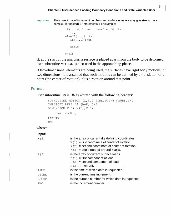
Chapter 2 User-defined Loading Boundary Conditions and State Variables User5
Important: The correct use of increment numbers and surface numbers may give rise to more complex (or nested) if statements. For example:
if(inc.eq.2 .and. nsurf.eq.3) then...
elseif(....) thenif(....) then
...endif
...endif
If, at the start of the analysis, a surface is placed apart from the body to be deformed, user subroutine MOTION is also used in the approaching phase.
If two-dimensional elements are being used, the surfaces have rigid body motions in two dimensions. It is assumed that such motions can be defined by a translation of a point (the center of rotation), plus a rotation around that point.
Format
User subroutine MOTION is written with the following headers:SUBROUTINE MOTION (X,F,V,TIME,DTIME,NSURF,INC)IMPLICIT REAL *8 (A-H, O-Z)DIMENSION X(*),V(*),F(*)
user coding
RETURNEND
where:
Input:X(3) is the array of current die defining coordinates.
X(1) = first coordinate of center of rotation.X(2) = second coordinate of center of rotation.X(3) = angle rotated around z-axis.
F(3) is the array of current surface loads.F(1) = first component of load.F(2) = second component of load.F(3) = moment.
TIME is the time at which data is requested.DTIME is the current time increment.NSURF is the surface number for which data is requested.INC is the increment number.

MSC.Marc Volume D: User Subroutines and Special Routines
6
Example
Assume that a rigid surface is identified as surface number 1, and is moving in the negative x-direction with a velocity of 1.0. The user subroutine MOTION can be written as follows:
SUBROUTINE MOTION(X,F,V,TIME,DTIME,NSURF,INC)IMPLICIT REAL *8 (A-H, O-Z)DIMENSION X(*),V(*),F(*)IF(NSURF.EQ.1) THEN
V(1)=-1.V(2)=0.V(3)=0.
ENDIFRETURNEND
Output:V(3) is the array of current surface velocities.
V(1) = first component of the velocity at the center of rotation.V(2) = second component of the velocity at the center of rotation.V(3) = angular velocity.
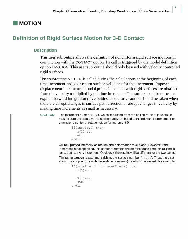
Chapter 2 User-defined Loading Boundary Conditions and State Variables User7
MOTION (3-D)
Definition of Rigid Surface Motion for 3-D Contact
Description
This user subroutine allows the definition of nonuniform rigid surface motions in conjunction with the CONTACT option. Its call is triggered by the model definition option UMOTION. This user subroutine should only be used with velocity controlled rigid surfaces.
User subroutine MOTION is called during the calculations at the beginning of each time increment and your return surface velocities for that increment. Imposed displacement increments at nodal points in contact with rigid surfaces are obtained from the velocity multiplied by the time increment. The surface path becomes an explicit forward integration of velocities. Therefore, caution should be taken when there are abrupt changes in surface path direction or abrupt changes in velocity by making time increments as small as necessary.
CAUTION: The increment number (inc), which is passed from the calling routine, is useful in making sure the data given is appropriately attributed to the relevant increments. For example, a center of rotation given for increment 0
if(inc.eq.0) thenx(1)=...etc.
endif
will be updated internally as motion and deformation take place. However, if the increment is not specified, this center of rotation will be reset each time this routine is read; that is, every increment. Obviously, the results will be different for the two cases.
The same caution is also applicable to the surface number (nsurf). Thus, the data should be coupled only with the surface number(s) for which it is meant. For example:
if(nsurf.eq.2 .or. nsurf.eq.4) thenx(1)=......v(1)=...etc.
endif
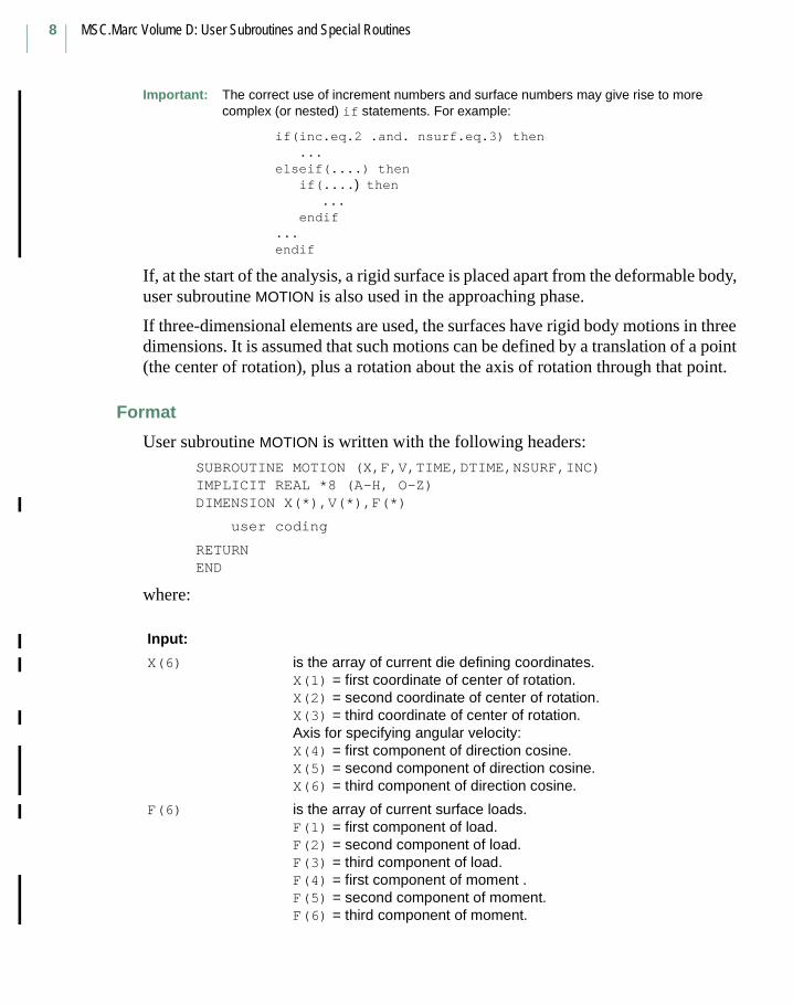
MSC.Marc Volume D: User Subroutines and Special Routines
8
Important: The correct use of increment numbers and surface numbers may give rise to more complex (or nested) if statements. For example:
if(inc.eq.2 .and. nsurf.eq.3) then...
elseif(....) thenif(....) then
...endif
...endif
If, at the start of the analysis, a rigid surface is placed apart from the deformable body, user subroutine MOTION is also used in the approaching phase.
If three-dimensional elements are used, the surfaces have rigid body motions in three dimensions. It is assumed that such motions can be defined by a translation of a point (the center of rotation), plus a rotation about the axis of rotation through that point.
Format
User subroutine MOTION is written with the following headers:SUBROUTINE MOTION (X,F,V,TIME,DTIME,NSURF,INC)IMPLICIT REAL *8 (A-H, O-Z)DIMENSION X(*),V(*),F(*)
user coding
RETURNEND
where:
Input:
X(6) is the array of current die defining coordinates.X(1) = first coordinate of center of rotation.X(2) = second coordinate of center of rotation.X(3) = third coordinate of center of rotation.Axis for specifying angular velocity:X(4) = first component of direction cosine.X(5) = second component of direction cosine.X(6) = third component of direction cosine.
F(6) is the array of current surface loads.F(1) = first component of load.F(2) = second component of load.F(3) = third component of load.F(4) = first component of moment .F(5) = second component of moment.F(6) = third component of moment.
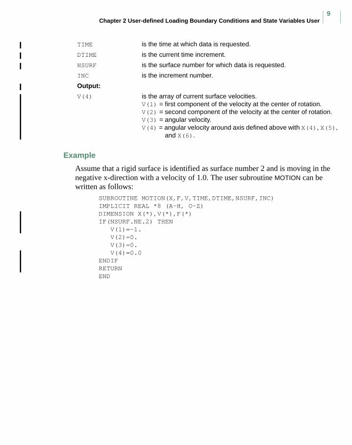
Chapter 2 User-defined Loading Boundary Conditions and State Variables User9
Example
Assume that a rigid surface is identified as surface number 2 and is moving in the negative x-direction with a velocity of 1.0. The user subroutine MOTION can be written as follows:
SUBROUTINE MOTION(X,F,V,TIME,DTIME,NSURF,INC)IMPLICIT REAL *8 (A-H, O-Z)DIMENSION X(*),V(*),F(*)IF(NSURF.NE.2) THEN
V(1)=-1.V(2)=0.V(3)=0.V(4)=0.0
ENDIFRETURNEND
TIME is the time at which data is requested.
DTIME is the current time increment.
NSURF is the surface number for which data is requested.
INC is the increment number.
Output:
V(4) is the array of current surface velocities.V(1) = first component of the velocity at the center of rotation.V(2) = second component of the velocity at the center of rotation.V(3) = angular velocity.V(4) = angular velocity around axis defined above with X(4), X(5),
and X(6).

MSC.Marc Volume D: User Subroutines and Special Routines
10
UHTCOE
Definition of Environment Film Coefficient
Description
This user subroutine allows the definition of variable film coefficients and sink temperatures of free surfaces, in conjunction with the CONTACT option and COUPLE parameter. Its call is triggered by the UHTCOEF option.
User subroutine UHTCOE is called at every element surface containing nodes that are on a free body boundary and for each surface at the trapezoidal rule integration points (that is, the nodes). These calls are made every iteration both during the assembly phase and the recovery phase of the heat transfer pass of a coupled analysis.
A distributed heat flux is being calculated according to the equation:
where:
By modifying H and TS, you can model varying heat transfer conditions along the boundary. Special attention has been given to provide you the capability of simulating radiation heat transfer, by making available the location and temperatures of all the surfaces in the environment.
You can either specify H and TS or specify the flux q directly which is treated strictly as such.
q is the heat flux entering the surface.
T is the surface temperature.
TS is the sink temperature.
H is the film coefficient.
q = H(T - TS)
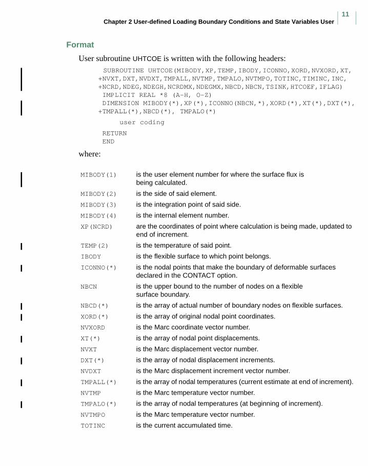
Chapter 2 User-defined Loading Boundary Conditions and State Variables User11
Format
User subroutine UHTCOE is written with the following headers:SUBROUTINE UHTCOE(MIBODY,XP,TEMP,IBODY,ICONNO,XORD,NVXORD,XT,
+NVXT,DXT,NVDXT,TMPALL,NVTMP,TMPALO,NVTMPO,TOTINC,TIMINC,INC,+NCRD,NDEG,NDEGH,NCRDMX,NDEGMX,NBCD,NBCN,TSINK,HTCOEF,IFLAG) IMPLICIT REAL *8 (A-H, O-Z) DIMENSION MIBODY(*),XP(*),ICONNO(NBCN,*),XORD(*),XT(*),DXT(*),+TMPALL(*),NBCD(*), TMPALO(*)
user coding
RETURN END
where:
MIBODY(1) is the user element number for where the surface flux is being calculated.
MIBODY(2) is the side of said element.
MIBODY(3) is the integration point of said side.
MIBODY(4) is the internal element number.
XP(NCRD) are the coordinates of point where calculation is being made, updated to end of increment.
TEMP(2) is the temperature of said point.
IBODY is the flexible surface to which point belongs.
ICONNO(*) is the nodal points that make the boundary of deformable surfaces declared in the CONTACT option.
NBCN is the upper bound to the number of nodes on a flexible surface boundary.
NBCD(*) is the array of actual number of boundary nodes on flexible surfaces.
XORD(*) is the array of original nodal point coordinates.
NVXORD is the Marc coordinate vector number.
XT(*) is the array of nodal point displacements.
NVXT is the Marc displacement vector number.
DXT(*) is the array of nodal displacement increments.
NVDXT is the Marc displacement increment vector number.
TMPALL(*) is the array of nodal temperatures (current estimate at end of increment).
NVTMP is the Marc temperature vector number.
TMPALO(*) is the array of nodal temperatures (at beginning of increment).
NVTMPO is the Marc temperature vector number.
TOTINC is the current accumulated time.

MSC.Marc Volume D: User Subroutines and Special Routines
12
TIMINC is the time increment.
INC is the increment number.
NCRD is the number of coordinates per node.
NDEG is the number of degrees of freedom per node.
NDEGH is the number of degrees of freedom for temperature (usually 1).
NCRDMX = NCRD unless different element types are in the model.
NDEGMX = NDEG unless different element types are in the model.
TSINK is the sink temperature declared in contact option for this flexible surface.
IFLAG =0 HTCOEF is a heat transfer coefficient =1 HTCOEF is a flux.
HTCOEF is the heat transfer coefficient between surface and environment, such that the heat flux per unit area that leaves the surface is:
Q = HTCOEF (TEMP - TSINK)orthe heat flux per unit area that leaves the surface.HTCOEF is to be defined here.

Chapter 3 User-defined Anistropy and Constitutive Relations User Subroutines13
Chapter 3 User-defined Anistropy
and Constitutive Relations User
Subroutines
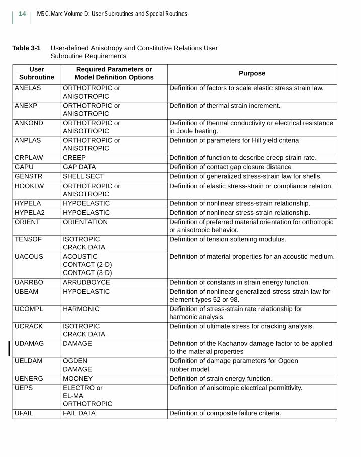
MSC.Marc Volume D: User Subroutines and Special Routines
14
Table 3-1 User-defined Anisotropy and Constitutive Relations User Subroutine Requirements
User Subroutine
Required Parameters or Model Definition Options
Purpose
ANELAS ORTHOTROPIC orANISOTROPIC
Definition of factors to scale elastic stress strain law.
ANEXP ORTHOTROPIC orANISOTROPIC
Definition of thermal strain increment.
ANKOND ORTHOTROPIC orANISOTROPIC
Definition of thermal conductivity or electrical resistance in Joule heating.
ANPLAS ORTHOTROPIC orANISOTROPIC
Definition of parameters for Hill yield criteria
CRPLAW CREEP Definition of function to describe creep strain rate.GAPU GAP DATA Definition of contact gap closure distanceGENSTR SHELL SECT Definition of generalized stress-strain law for shells.HOOKLW ORTHOTROPIC or
ANISOTROPICDefinition of elastic stress-strain or compliance relation.
HYPELA HYPOELASTIC Definition of nonlinear stress-strain relationship.HYPELA2 HYPOELASTIC Definition of nonlinear stress-strain relationship.ORIENT ORIENTATION Definition of preferred material orientation for orthotropic
or anisotropic behavior.TENSOF ISOTROPIC
CRACK DATADefinition of tension softening modulus.
UACOUS ACOUSTICCONTACT (2-D)CONTACT (3-D)
Definition of material properties for an acoustic medium.
UARRBO ARRUDBOYCE Definition of constants in strain energy function.UBEAM HYPOELASTIC Definition of nonlinear generalized stress-strain law for
element types 52 or 98.UCOMPL HARMONIC Definition of stress-strain rate relationship for
harmonic analysis.UCRACK ISOTROPIC
CRACK DATADefinition of ultimate stress for cracking analysis.
UDAMAG DAMAGE Definition of the Kachanov damage factor to be applied to the material properties
UELDAM OGDENDAMAGE
Definition of damage parameters for Ogden rubber model.
UENERG MOONEY Definition of strain energy function.UEPS ELECTRO or
EL-MAORTHOTROPIC
Definition of anisotropic electrical permittivity.
UFAIL FAIL DATA Definition of composite failure criteria.
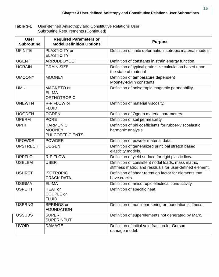
Chapter 3 User-defined Anistropy and Constitutive Relations User Subroutines15
UFINITE PLASTICITY orELASTICITY
Definition of finite deformation isotropic material models.
UGENT ARRUDBOYCE Definition of constants in strain energy function.UGRAIN GRAIN SIZE Definition of typical grain size calculation based upon
the state of materialUMOONY MOONEY Definition of temperature dependent
Mooney-Rivlin constants.UMU MAGNETO or
EL-MAORTHOTROPIC
Definition of anisotropic magnetic permeability.
UNEWTN R-P FLOW orFLUID
Definition of material viscosity.
UOGDEN OGDEN Definition of Ogden material parameters.UPERM PORE Definition of soil permeability.UPHI HARMONIC
MOONEYPHI-COEFFICIENTS
Definition of phi coefficients for rubber-viscoelastic harmonic analysis.
UPOWDR POWDER Definition of powder material data.UPSTRECH ODGEN Definition of generalized principal stretch based
elasticity models.URPFLO R-P FLOW Definition of yield surface for rigid plastic flow.USELEM USER Definition of consistent nodal loads, mass matrix,
stiffness matrix, and residuals for user-defined element.USHRET ISOTROPIC
CRACK DATADefinition of shear retention factor for elements that have cracks.
USIGMA EL-MA Definition of anisotropic electrical conductivity.USPCHT HEAT or
COUPLE orFLUID
Definition of specific heat.
USPRNG SPRINGS orFOUNDATION
Definition of nonlinear spring or foundation stiffness.
USSUBS SUPERSUPERINPUT
Definition of superelements not generated by Marc.
UVOID DAMAGE Definition of initial void fraction for Gurson damage model.
Table 3-1 User-defined Anisotropy and Constitutive Relations User Subroutine Requirements (Continued)
User Subroutine
Required Parameters or Model Definition Options
Purpose

MSC.Marc Volume D: User Subroutines and Special Routines
16
UVOIDN DAMAGE Definition of void nucleation for Gurson damage model.VSWELL CREEP Definition of volumetric swelling.WKSLP ISOTROPIC or
ORTHOTROPIC orANISOTROPICWORK HARD
Definition of work hardening or strain hardening data.
Table 3-1 User-defined Anisotropy and Constitutive Relations User Subroutine Requirements (Continued)
User Subroutine
Required Parameters or Model Definition Options
Purpose
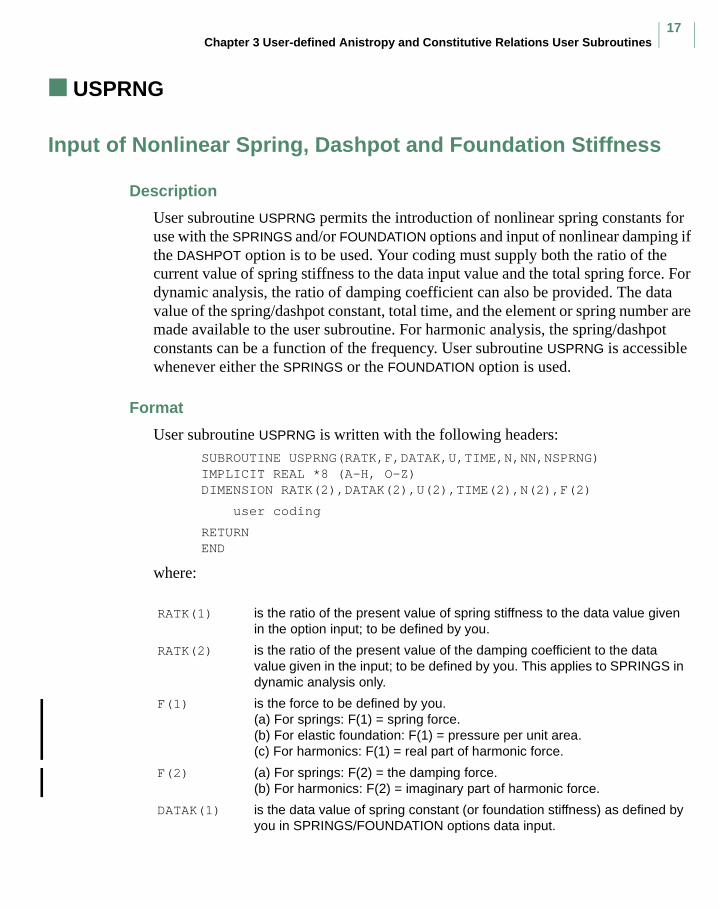
Chapter 3 User-defined Anistropy and Constitutive Relations User Subroutines17
USPRNG
Input of Nonlinear Spring, Dashpot and Foundation Stiffness
Description
User subroutine USPRNG permits the introduction of nonlinear spring constants for use with the SPRINGS and/or FOUNDATION options and input of nonlinear damping if the DASHPOT option is to be used. Your coding must supply both the ratio of the current value of spring stiffness to the data input value and the total spring force. For dynamic analysis, the ratio of damping coefficient can also be provided. The data value of the spring/dashpot constant, total time, and the element or spring number are made available to the user subroutine. For harmonic analysis, the spring/dashpot constants can be a function of the frequency. User subroutine USPRNG is accessible whenever either the SPRINGS or the FOUNDATION option is used.
Format
User subroutine USPRNG is written with the following headers:SUBROUTINE USPRNG(RATK,F,DATAK,U,TIME,N,NN,NSPRNG)IMPLICIT REAL *8 (A-H, O-Z)DIMENSION RATK(2),DATAK(2),U(2),TIME(2),N(2),F(2)
user coding
RETURNEND
where:
RATK(1) is the ratio of the present value of spring stiffness to the data value given in the option input; to be defined by you.
RATK(2) is the ratio of the present value of the damping coefficient to the data value given in the input; to be defined by you. This applies to SPRINGS in dynamic analysis only.
F(1) is the force to be defined by you.(a) For springs: F(1) = spring force.(b) For elastic foundation: F(1) = pressure per unit area.(c) For harmonics: F(1) = real part of harmonic force.
F(2) (a) For springs: F(2) = the damping force.(b) For harmonics: F(2) = imaginary part of harmonic force.
DATAK(1) is the data value of spring constant (or foundation stiffness) as defined by you in SPRINGS/FOUNDATION options data input.
MSC.Marc Volume D: User Subroutines and Special Routines
18
If the user subroutine is called for an elastic foundation point, NSPRNG is zero.
If the user subroutine is called for a spring, N and NN are zero.
Note that if you prefer to give the absolute value of the spring constant rather than a ratio, the corresponding value in the SPRINGS or FOUNDATION option should be set to 1. The same applies for a damping constant.
DATAK(2) is the data value of the damping constant as defined by you in the SPRINGS option data input.
For elastic foundation (only static contribution):
U(1) For elastic foundation: U(1) = Un.
(positive in the direction specified by face identification given in the FOUNDATION option).
U(2)-U(4) not used
For springs/dashpots (static and/or dynamic contribution):
U(1) For springs: .
U(2) For dynamic spring/dashpot .
U(3)-U(4) not used
For springs/dashpots (harmonic analysis):
U(1) static predeformation
U(2) not used
U(3) real part of harmonic deformation.
U(4) imaginary part of harmonic deformation
TIME(1) is the total time (for dynamic or creep analysis).
TIME(2) is the frequency (for harmonic analysis with spring/dashpot).
N(1) is the element number (only for elastic foundation).
N(2) is the face number (only for elastic foundation).
NN is the integration point number (only for elastic foundation).
NSPRNG is the spring number, the position of the spring in the input data list (only for springs).
U 1( ) U2 U1–=
U 2( ) U·
2 U·
1–=
U 1( ) U2 U1–=
U 3( ) U2 U1–=
U 4( ) U2 U1–=
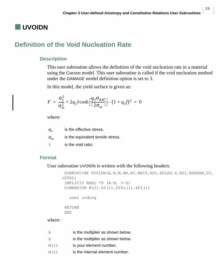
Chapter 3 User-defined Anistropy and Constitutive Relations User Subroutines19
UVOIDN
Definition of the Void Nucleation Rate
Description
This user subroutine allows the definition of the void nucleation rate in a material using the Gurson model. This user subroutine is called if the void nucleation method under the DAMAGE model definition option is set to 3.
In this model, the yield surface is given as:
where:
Format
User subroutine UVOIDN is written with the following headers: SUBROUTINE UVOIDN(A,B,M,NN,KC,MATS,EPL,EPLAS,S,NDI,NSHEAR,DT,+DTDL) IMPLICIT REAL *8 (A-H, O-Z) DIMENSION M(2),DT(1),DTDL(1),EPL(1) user coding RETURN END
where:
σe is the effective stress.
σm is the equivalent tensile stress.
f is the void ratio.
A is the multiplier as shown below.
B is the multiplier as shown below.
M(1) is your element number.
M(2) is the internal element number.
Fσe
2
σm2
------- 2q1fq2σKK
2σm---------------
cosh 1 q1f+( )2–+ 0= =

MSC.Marc Volume D: User Subroutines and Special Routines
20
In this user subroutine, the following type of stress controlled nucleation rate can be specified:
where is the von Mises equivalent stress rate, and is the hydrostatic stress rate.
NN is the integration point number.
KC is the layer number.
MATS is the material id.
EPL is the plastic strain components.
EPLAS is the equivalent plastic strain.
S is the stress array.
NDI is the number of direct components.
NSHEAR is the number of shear components.
DT is the array of state variables, temperature first.
DTDL is the array of increment of state variables.
f· Aσ·
Bσ· kk
3--------+=
σ·
σ· kk
Chapter 3 User-defined Anistropy and Constitutive Relations User Subroutines21
UDAMAG
Prediction of Material Damage
Description
This user subroutine provides you with the mechanism for providing a Kachanov damage factor to be applied to the material properties. UDAMAG is used in conjunction with the DAMAGE model definition option. You define the damage factor (df). 0 ≤ df ≤ 1 where df = 0 implies a fully damaged material. If model 9 is used, then:
If model 10 is used, then:
Format
User subroutine UDAMAG is written with the following header lines:
SUBROUTINE UDAMAG(M,N,NN,KC,MATS,EPLAS,ERATE,DT,DTDl,*DAMDAT,DAMFAC,TIME,DELTIME) IMPLICIT REAL*8 (A-H,O-Z) DIMENSION DT (*),DAMDAT(*) user coding RETURN END
where:
M is the element number.
N is the elsto number.
NN is the integration point number.
KC is the layer.
MATS is the material id.
EPLAS is the equivalent plastic strain.
ERATE is the equivalent plastic strain rate.
DT is the state variables at beginning of increment.
DTDL is the incremental state variables.
DAMDAT is the material data, DAMDAT (1) is the initial damage factor.
σy σy εp ε· p
T, ,( )* 1.0 df–( )=
σy σy εp ε· p
T, ,( )* 1.0 df–( ) and E = E T( )* 1.0 df–( )=

MSC.Marc Volume D: User Subroutines and Special Routines
22
DAMFAC is the current damage factor.
TIME is the time - beginning of increment.
DELTIME is the incremental time.
Chapter 3 User-defined Anistropy and Constitutive Relations User Subroutines23
USELEM
User-defined Element
Description
This user subroutine allows you to calculate your own finite element stiffness or mass matrix. This can also be used as interface with other numerical techniques. In general, in the finite element calculation, several matrices are required; hence, for a particular element, this user subroutine is called a multiple number of times. The calls and your requirements are defined as follows:
To use this option, the USER parameter must be included to define the size of the element stiffness matrix and other critical dimensions and the element type given on the connectivity must be a negative number.
IFLAG=1 Return the equivalent nodal loads (F) given distributed surface or body loads. If the ELASTIC, FOLLOW FOR parameters or the AUTO STEP, AUTO TIME, AUTO INCREMENT options are used, these are total loads or else incremental loads. In a heat transfer analysis, this is the total flux vector.
IFLAG=2 Return the element tangent stiffness matrix (K). For an elastic analysis, this is the usual stiffness. For a heat transfer matrix analysis, this is the conductivity matrix. Also calculate the total internal forces (R). This is not necessary in a linear elastic analysis if the LOAD COR parameter has been turned off.
IFLAG=3 Return the mass matrix (M) for a dynamic analysis or specific heat matrix for a heat transfer problem.
IFLAG=4 Calculate the incremental strains (DE), generalized stresses (GSIGS) and the internal force (R). For a linear elastic solution, if only displacements are required, you do not need to return any values.
IFLAG=5 Output element results if so desired.
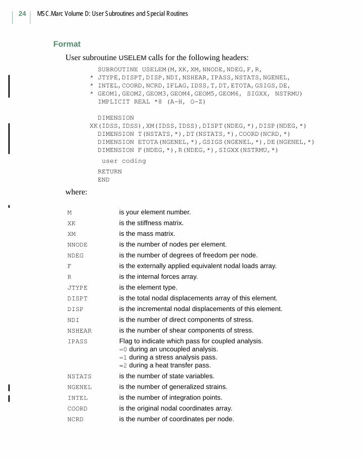
MSC.Marc Volume D: User Subroutines and Special Routines
24
Format
User subroutine USELEM calls for the following headers: SUBROUTINE USELEM(M,XK,XM,NNODE,NDEG,F,R,* JTYPE,DISPT,DISP,NDI,NSHEAR,IPASS,NSTATS,NGENEL,* INTEL,COORD,NCRD,IFLAG,IDSS,T,DT,ETOTA,GSIGS,DE,* GEOM1,GEOM2,GEOM3,GEOM4,GEOM5,GEOM6, SIGXX, NSTRMU) IMPLICIT REAL *8 (A-H, O-Z) DIMENSION XK(IDSS,IDSS),XM(IDSS,IDSS),DISPT(NDEG,*),DISP(NDEG,*) DIMENSION T(NSTATS,*),DT(NSTATS,*),COORD(NCRD,*) DIMENSION ETOTA(NGENEL,*),GSIGS(NGENEL,*),DE(NGENEL,*) DIMENSION F(NDEG,*),R(NDEG,*),SIGXX(NSTRMU,*)
user coding
RETURN END
where:
M is your element number.
XK is the stiffness matrix.
XM is the mass matrix.
NNODE is the number of nodes per element.
NDEG is the number of degrees of freedom per node.
F is the externally applied equivalent nodal loads array.
R is the internal forces array.
JTYPE is the element type.
DISPT is the total nodal displacements array of this element.
DISP is the incremental nodal displacements of this element.
NDI is the number of direct components of stress.
NSHEAR is the number of shear components of stress.
IPASS Flag to indicate which pass for coupled analysis.=0 during an uncoupled analysis.=1 during a stress analysis pass.=2 during a heat transfer pass.
NSTATS is the number of state variables.
NGENEL is the number of generalized strains.
INTEL is the number of integration points.
COORD is the original nodal coordinates array.
NCRD is the number of coordinates per node.

Chapter 3 User-defined Anistropy and Constitutive Relations User Subroutines25
Note that the stiffness matrix is normally symmetric. If a nonsymmetric formulation is used, the SOLVER option should be used to indicate this.
IFLAG indicates what is to be returned by you.=1 Called by OPRESS during formation of load vector.
You return F.=2 Called by OASEMB during formation of stiffness matrix.
You return XK,R.=3 Called by OASMAS during formation of mass matrix.
You return XM.=4 Called by OGETST during stress recovery.
You return R,GSIGS,DE,ETOTA,SIGXX.=5 Called by SCIMP during output phase.
You print results.
IDSS is the size of element stiffness matrix.
T is the state variables.
DT is the increment of state variables.
ETOTA is the total strain array.
GSIGS is the generalized stress array.
DE is the increment of strain array.
GEOM1 is the first geometric parameter.
GEOM2 is the second geometric parameter.
GEOM3 is the third geometric parameter.
GEOM4 is the fourth geometric parameter.
GEOM5 is the fifth geometric parameter.
GEOM6 is the sixth geometric parameter.
SIGXX is layer stresses for shell elements and is equal to GSIGS for continuum element.
NSTRMU is the number of stresses per integration points.
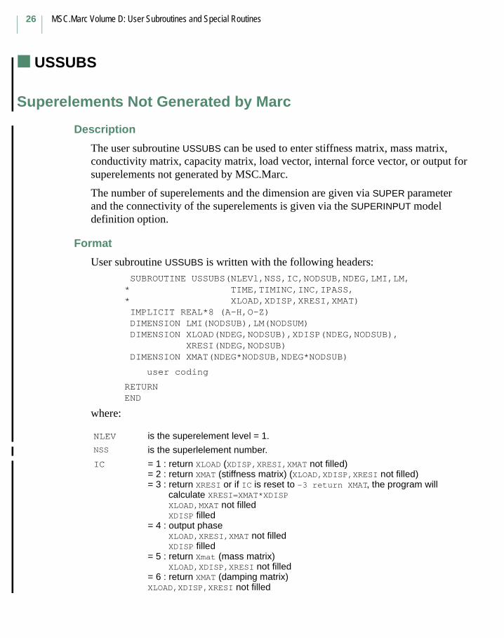
MSC.Marc Volume D: User Subroutines and Special Routines
26
USSUBS
Superelements Not Generated by Marc
Description
The user subroutine USSUBS can be used to enter stiffness matrix, mass matrix, conductivity matrix, capacity matrix, load vector, internal force vector, or output for superelements not generated by MSC.Marc.
The number of superelements and the dimension are given via SUPER parameter and the connectivity of the superelements is given via the SUPERINPUT model definition option.
Format
User subroutine USSUBS is written with the following headers:SUBROUTINE USSUBS(NLEVl,NSS,IC,NODSUB,NDEG,LMI,LM,
* TIME,TIMINC,INC,IPASS,* XLOAD,XDISP,XRESI,XMAT)IMPLICIT REAL*8 (A-H,O-Z)DIMENSION LMI(NODSUB),LM(NODSUM)DIMENSION XLOAD(NDEG,NODSUB),XDISP(NDEG,NODSUB),
XRESI(NDEG,NODSUB)DIMENSION XMAT(NDEG*NODSUB,NDEG*NODSUB)
user coding
RETURNEND
where:
NLEV is the superelement level = 1.NSS is the superlelement number.
IC = 1 : return XLOAD (XDISP,XRESI,XMAT not filled)= 2 : return XMAT (stiffness matrix) (XLOAD,XDISP,XRESI not filled)= 3 : return XRESI or if IC is reset to -3 return XMAT, the program will
calculate XRESI=XMAT*XDISP XLOAD,MXAT not filled XDISP filled
= 4 : output phase XLOAD,XRESI,XMAT not filled XDISP filled
= 5 : return Xmat (mass matrix)XLOAD,XDISP,XRESI not filled
= 6 : return XMAT (damping matrix)XLOAD,XDISP,XRESI not filled

Chapter 3 User-defined Anistropy and Constitutive Relations User Subroutines27
NODSUM is the number of nodes in the superelement.
NDEG is the number of degrees of freedom per node in the superelement.
LIM() is the node id’s of the superelement.
LM() is the future expansion.
TIME is the transient time at the start of the increment.
TIMINC is the incremental time period.
INC is the increment number.
IPASS 0 - not a coupled analysis.1 - coupled analysis, stress pass2 - coupled analysis, heat transfer pass
XLOAD() is the external load vector on the superelement; this is total external force.XDISP() is the displacement of the superelement.XRESI() in the internal force vector for the superelement
XRESI-XMAT*XDISP (if linear)XMAT() is the stiffness, mass, damping matrix of the superelement.

MSC.Marc Volume D: User Subroutines and Special Routines
28
Chapter 6 Geometry Modifications
User Subroutines
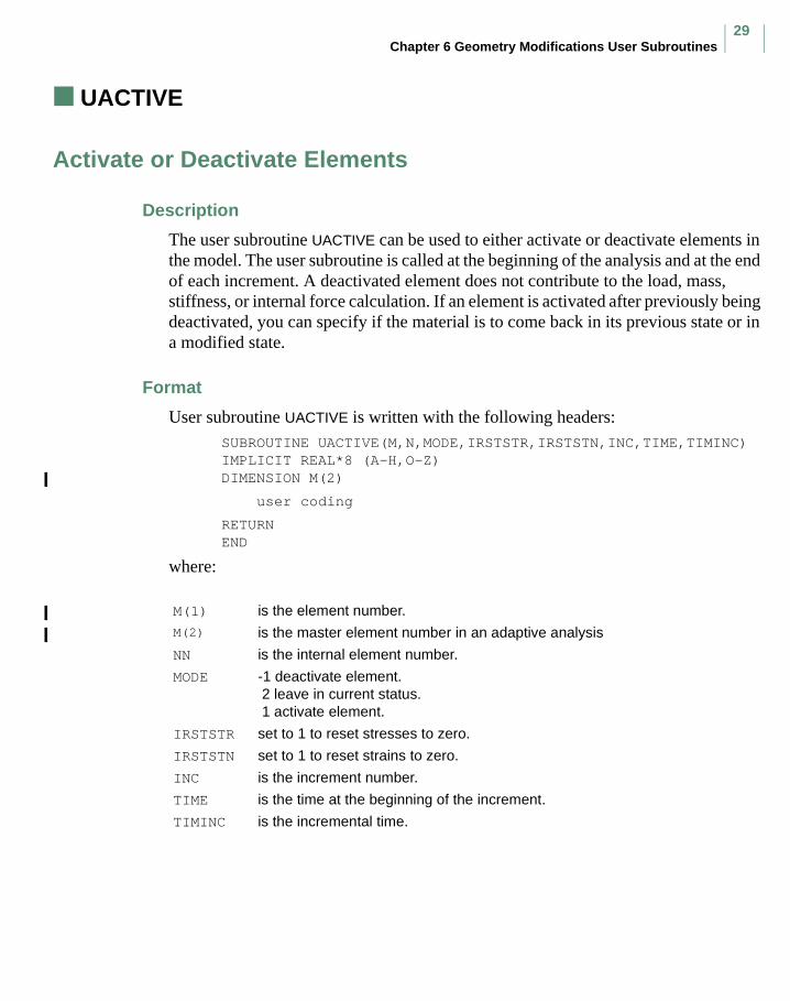
Chapter 6 Geometry Modifications User Subroutines29
UACTIVE
Activate or Deactivate Elements
Description
The user subroutine UACTIVE can be used to either activate or deactivate elements in the model. The user subroutine is called at the beginning of the analysis and at the end of each increment. A deactivated element does not contribute to the load, mass, stiffness, or internal force calculation. If an element is activated after previously being deactivated, you can specify if the material is to come back in its previous state or in a modified state.
Format
User subroutine UACTIVE is written with the following headers:SUBROUTINE UACTIVE(M,N,MODE,IRSTSTR,IRSTSTN,INC,TIME,TIMINC)IMPLICIT REAL*8 (A-H,O-Z)DIMENSION M(2)
user coding
RETURNEND
where:
M(1) is the element number.M(2) is the master element number in an adaptive analysis
NN is the internal element number.
MODE -1 deactivate element.2 leave in current status.1 activate element.
IRSTSTR set to 1 to reset stresses to zero.
IRSTSTN set to 1 to reset strains to zero.
INC is the increment number.
TIME is the time at the beginning of the increment.
TIMINC is the incremental time.

MSC.Marc Volume D: User Subroutines and Special Routines
30
Chapter 7 Output Quantities User Subroutines
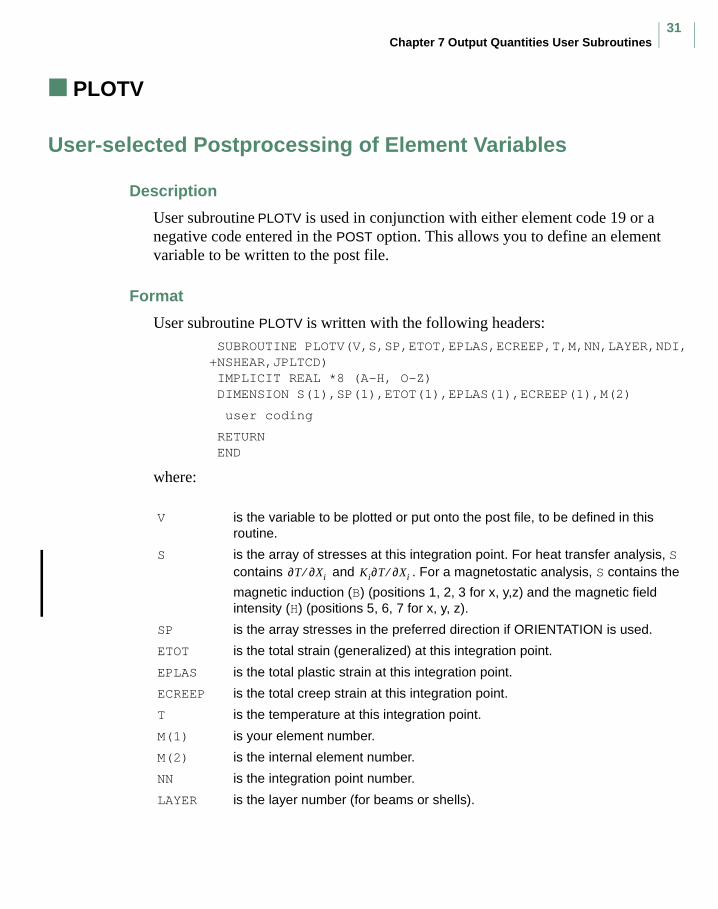
Chapter 7 Output Quantities User Subroutines31
PLOTV
User-selected Postprocessing of Element Variables
Description
User subroutine PLOTV is used in conjunction with either element code 19 or a negative code entered in the POST option. This allows you to define an element variable to be written to the post file.
Format
User subroutine PLOTV is written with the following headers: SUBROUTINE PLOTV(V,S,SP,ETOT,EPLAS,ECREEP,T,M,NN,LAYER,NDI, +NSHEAR,JPLTCD) IMPLICIT REAL *8 (A-H, O-Z) DIMENSION S(1),SP(1),ETOT(1),EPLAS(1),ECREEP(1),M(2)
user coding
RETURN END
where:
V is the variable to be plotted or put onto the post file, to be defined in this routine.
S is the array of stresses at this integration point. For heat transfer analysis, S contains and . For a magnetostatic analysis, S contains the
magnetic induction (B) (positions 1, 2, 3 for x, y,z) and the magnetic field intensity (H) (positions 5, 6, 7 for x, y, z).
SP is the array stresses in the preferred direction if ORIENTATION is used.
ETOT is the total strain (generalized) at this integration point.
EPLAS is the total plastic strain at this integration point.
ECREEP is the total creep strain at this integration point.
T is the temperature at this integration point.
M(1) is your element number.
M(2) is the internal element number.
NN is the integration point number.
LAYER is the layer number (for beams or shells).
∂T ∂Xi⁄ Ki∂T ∂Xi⁄
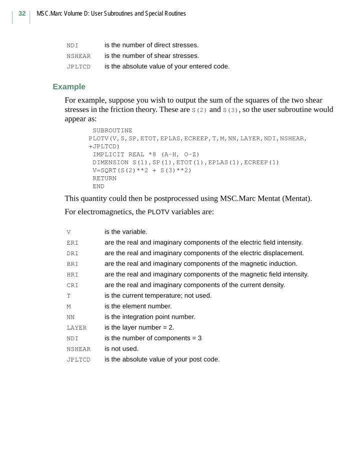
MSC.Marc Volume D: User Subroutines and Special Routines
32
Example
For example, suppose you wish to output the sum of the squares of the two shear stresses in the friction theory. These are S(2) and S(3), so the user subroutine would appear as:
SUBROUTINE PLOTV(V,S,SP,ETOT,EPLAS,ECREEP,T,M,NN,LAYER,NDI,NSHEAR,+JPLTCD) IMPLICIT REAL *8 (A-H, O-Z) DIMENSION S(1),SP(1),ETOT(1),EPLAS(1),ECREEP(1) V=SQRT(S(2)**2 + S(3)**2) RETURN END
This quantity could then be postprocessed using MSC.Marc Mentat (Mentat).
For electromagnetics, the PLOTV variables are:
NDI is the number of direct stresses.
NSHEAR is the number of shear stresses.
JPLTCD is the absolute value of your entered code.
V is the variable.
ERI are the real and imaginary components of the electric field intensity.
DRI are the real and imaginary components of the electric displacement.
BRI are the real and imaginary components of the magnetic induction.
HRI are the real and imaginary components of the magnetic field intensity.
CRI are the real and imaginary components of the current density.
T is the current temperature; not used.
M is the element number.
NN is the integration point number.
LAYER is the layer number = 2.
NDI is the number of components = 3
NSHEAR is not used.
JPLTCD is the absolute value of your post code.

Chapter 9 Special Routines — Marc Post File Processor33
Chapter 9 Special Routines —
Marc Post File Processor
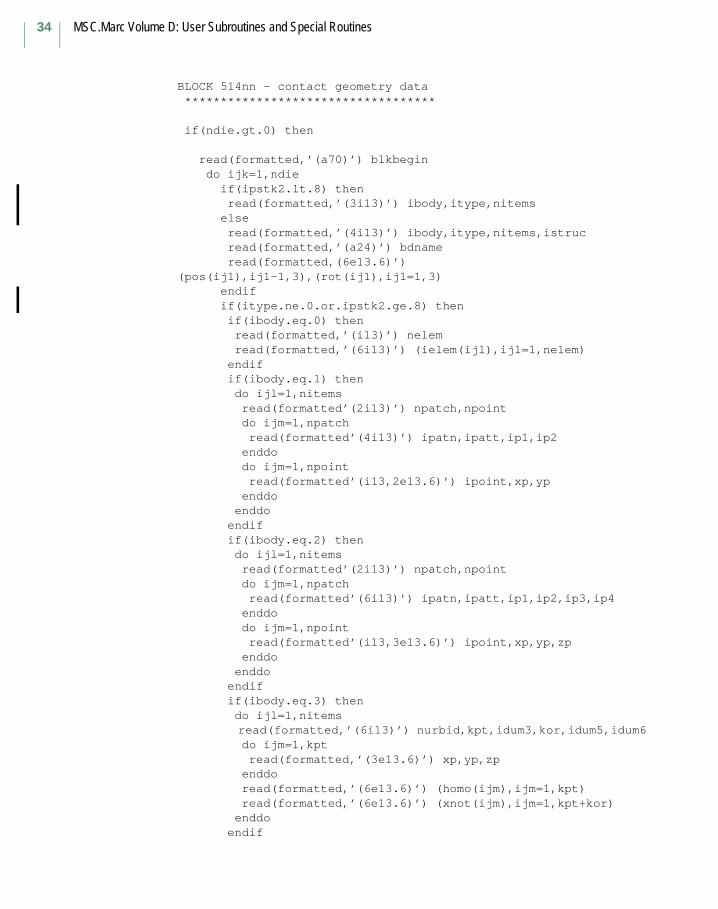
MSC.Marc Volume D: User Subroutines and Special Routines
34
BLOCK 514nn - contact geometry data *********************************** if(ndie.gt.0) then
read(formatted,’(a70)’) blkbegin do ijk=1,ndie
if(ipstk2.lt.8) thenread(formatted,’(3i13)’) ibody,itype,nitemselseread(formatted,’(4i13)’) ibody,itype,nitems,istrucread(formatted,’(a24)’) bdnameread(formatted,(6e13.6)’)
(pos(ij1),ij1-1,3),(rot(ij1),ij1=1,3)endifif(itype.ne.0.or.ipstk2.ge.8) then
if(ibody.eq.0) then read(formatted,’(i13)’) nelem read(formatted,’(6i13)’) (ielem(ijl),ijl=1,nelem) endif if(ibody.eq.1) then do ijl=1,nitems read(formatted’(2i13)’) npatch,npoint do ijm=1,npatch read(formatted’(4i13)’) ipatn,ipatt,ip1,ip2 enddo do ijm=1,npoint read(formatted’(i13,2e13.6)’) ipoint,xp,yp enddo enddo endif if(ibody.eq.2) then do ijl=1,nitems read(formatted’(2i13)’) npatch,npoint do ijm=1,npatch read(formatted’(6i13)’) ipatn,ipatt,ip1,ip2,ip3,ip4 enddo do ijm=1,npoint read(formatted’(i13,3e13.6)’) ipoint,xp,yp,zp enddo enddo endif if(ibody.eq.3) then do ijl=1,nitems read(formatted,’(6i13)’) nurbid,kpt,idum3,kor,idum5,idum6 do ijm=1,kpt read(formatted,’(3e13.6)’) xp,yp,zp enddo read(formatted,’(6e13.6)’) (homo(ijm),ijm=1,kpt) read(formatted,’(6e13.6)’) (xnot(ijm),ijm=1,kpt+kor) enddo endif
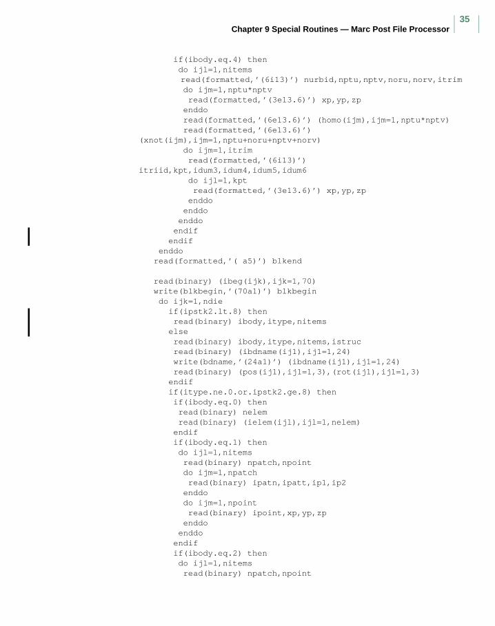
Chapter 9 Special Routines — Marc Post File Processor35
if(ibody.eq.4) then do ijl=1,nitems read(formatted,’(6i13)’) nurbid,nptu,nptv,noru,norv,itrim do ijm=1,nptu*nptv read(formatted,’(3e13.6)’) xp,yp,zp enddo read(formatted,’(6e13.6)’) (homo(ijm),ijm=1,nptu*nptv) read(formatted,’(6e13.6)’) (xnot(ijm),ijm=1,nptu+noru+nptv+norv) do ijm=1,itrim read(formatted,’(6i13)’) itriid,kpt,idum3,idum4,idum5,idum6 do ijl=1,kpt read(formatted,’(3e13.6)’) xp,yp,zp enddo enddo enddo endif endif enddo read(formatted,’( a5)’) blkend
read(binary) (ibeg(ijk),ijk=1,70) write(blkbegin,’(70a1)’) blkbegin do ijk=1,ndie
if(ipstk2.lt.8) thenread(binary) ibody,itype,nitemselseread(binary) ibody,itype,nitems,istrucread(binary) (ibdname(ij1),ij1=1,24)write(bdname,’(24a1)’) (ibdname(ij1),ij1=1,24)read(binary) (pos(ij1),ij1=1,3),(rot(ij1),ij1=1,3)endifif(itype.ne.0.or.ipstk2.ge.8) then
if(ibody.eq.0) then read(binary) nelem read(binary) (ielem(ijl),ijl=1,nelem) endif if(ibody.eq.1) then do ijl=1,nitems read(binary) npatch,npoint do ijm=1,npatch read(binary) ipatn,ipatt,ip1,ip2 enddo do ijm=1,npoint read(binary) ipoint,xp,yp,zp enddo enddo endif if(ibody.eq.2) then do ijl=1,nitems read(binary) npatch,npoint
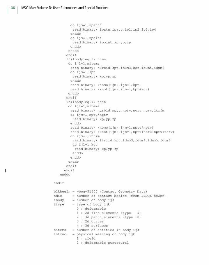
MSC.Marc Volume D: User Subroutines and Special Routines
36
do ijm=1,npatch read(binary) ipatn,ipatt,ip1,ip2,ip3,ip4 enddo do ijm=1,npoint read(binary) ipoint,xp,yp,zp enddo enddo endif if(ibody.eq.3) then do ijl=1,nitems read(binary) nurbid,kpt,idum3,kor,idum5,idum6 do ijm=1,kpt read(binary) xp,yp,zp enddo read(binary) (homo(ijm),ijm=1,kpt) read(binary) (xnot(ijm),ijm=1,kpt+kor) enddo endif if(ibody.eq.4) then do ijl=1,nitems read(binary) nurbid,nptu,nptv,noru,norv,itrim do ijm=1,nptu*nptv read(binary) xp,yp,zp enddo read(binary) (homo(ijm),ijm=1,nptu*nptv) read(binary) (xnot(ijm),ijm=1,nptu+noru+nptv+norv) do ijm=1,itrim read(binary) itriid,kpt,idum3,idum4,idum5,idum6 do ijl=1,kpt read(binary) xp,yp,zp enddo enddo enddo endif endif enddo
endif
blkbegin = =beg=51400 (Contact Geometry Data) ndie = number of contact bodies (from BLOCK 502nn) ibody = number of body ijk itype = type of body ijk 0 : deformable 1 : 2d line elements (type 9) 2 : 3d patch elements (type 18) 3 : 2d curves 4 : 3d surfaces nitems = number of entities in body ijk istruc = physical meaning of body ijk 1 : rigid 2 : deformable structural
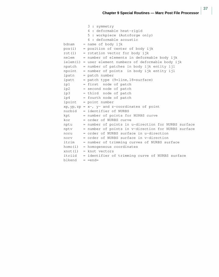
Chapter 9 Special Routines — Marc Post File Processor37
3 : symmetry 4 : deformable heat-rigid 5 : workpiece (Autoforge only) 6 : deformable acoustic bdnam = name of body ijk pos(i) = position of center of body ijk rot(i) = rotation vector for body ijk nelem = number of elements in deformable body ijk ielem(i) = user element numbers of deformable body ijk npatch = number of patches in body ijk entity ijl npoint = number of points in body ijk entity ijl ipatn = patch number ipatt = patch type (9=line,18=surface) ip1 = first node of patch ip2 = second node of patch ip3 = third node of patch ip4 = fourth node of patch ipoint = point number xp,yp,zp = x-, y- and z-coordinates of point nurbid = identifier of NURBS kpt = number of points for NURBS curve kor = order of NURBS curve nptu = number of points in u-direction for NURBS surface nptv = number of points in v-direction for NURBS surface noru = order of NURBS surface in u-direction norv = order of NURBS surface in v-direction itrim = number of trimming curves of NURBS surface homo(i) = homogeneous coordinates xnot(i) = knot vectors itriid = identifier of trimming curve of NURBS surface blkend = =end=
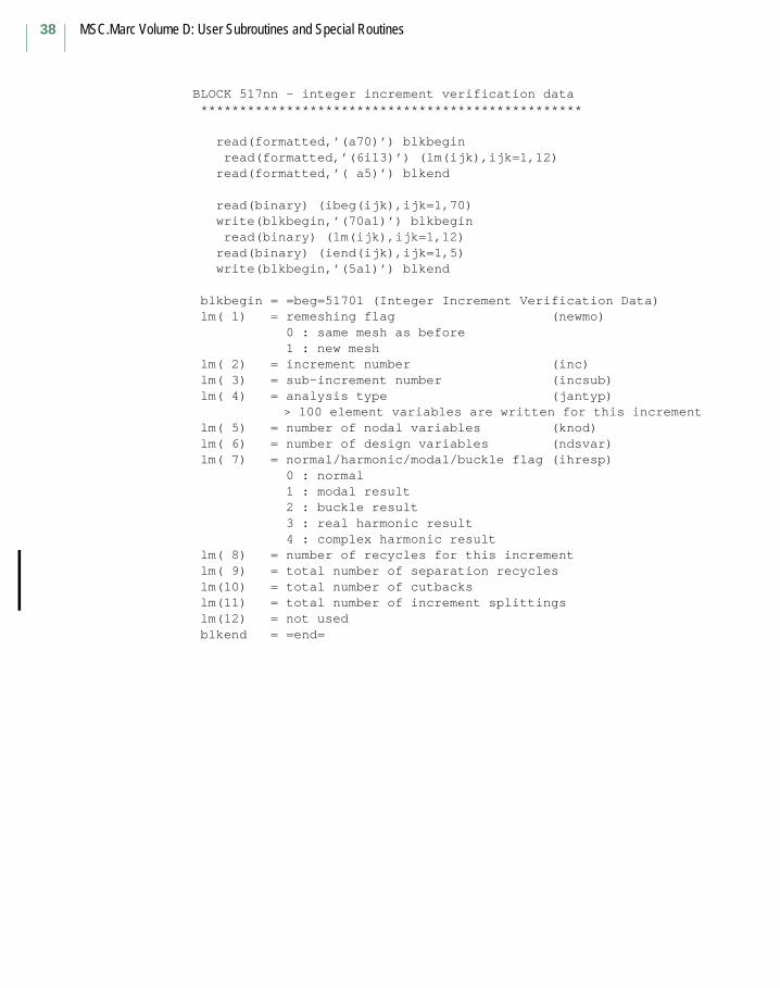
MSC.Marc Volume D: User Subroutines and Special Routines
38
BLOCK 517nn - integer increment verification data *************************************************
read(formatted,’(a70)’) blkbegin read(formatted,’(6i13)’) (lm(ijk),ijk=1,12) read(formatted,’( a5)’) blkend
read(binary) (ibeg(ijk),ijk=1,70) write(blkbegin,’(70a1)’) blkbegin read(binary) (lm(ijk),ijk=1,12) read(binary) (iend(ijk),ijk=1,5) write(blkbegin,’(5a1)’) blkend
blkbegin = =beg=51701 (Integer Increment Verification Data) lm( 1) = remeshing flag (newmo) 0 : same mesh as before 1 : new mesh lm( 2) = increment number (inc) lm( 3) = sub-increment number (incsub) lm( 4) = analysis type (jantyp) > 100 element variables are written for this increment lm( 5) = number of nodal variables (knod) lm( 6) = number of design variables (ndsvar) lm( 7) = normal/harmonic/modal/buckle flag (ihresp) 0 : normal 1 : modal result 2 : buckle result 3 : real harmonic result 4 : complex harmonic result lm( 8) = number of recycles for this increment lm( 9) = total number of separation recycles lm(10) = total number of cutbacks lm(11) = total number of increment splittings lm(12) = not used blkend = =end=
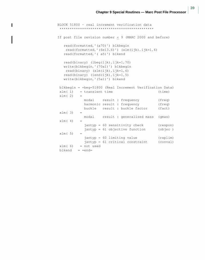
Chapter 9 Special Routines — Marc Post File Processor39
BLOCK 51800 - real increment verification data **********************************************
If post file revision number < 9 (MARC 2000 and before)
read(formatted,’(a70)’) blkbegin read(formatted,’(6e13.6)’) (xlm(ijk),ijk=1,6) read(formatted,’( a5)’) blkend
read(binary) (ibeg(ijk),ijk=1,70) write(blkbegin,’(70a1)’) blkbegin read(binary) (xlm(ijk),ijk=1,6) read(binary) (iend(ijk),ijk=1,5) write(blkbegin,’(5a1)’) blkend
blkbegin = =beg=51800 (Real Increment Verification Data) xlm( 1) = transient time (time) xlm( 2) = modal result : frequency (freq) harmonic result : frequency (freq) buckle result : buckle factor (fact) xlm( 3) = modal result : generalized mass (gmas) xlm( 4) = jantyp = 60 sensitivity check (respon) jantyp = 61 objective function (objec ) xlm( 5) = jantyp = 60 limiting value (rsplim) jantyp = 61 critical constraint (conval) xlm( 6) = not used blkend = =end=
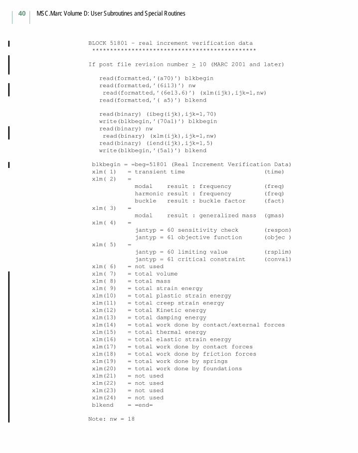
MSC.Marc Volume D: User Subroutines and Special Routines
40
BLOCK 51801 - real increment verification data **********************************************
If post file revision number > 10 (MARC 2001 and later)
read(formatted,’(a70)’) blkbegin read(formatted,’(6i13)’) nw
read(formatted,’(6e13.6)’) (xlm(ijk),ijk=1,nw) read(formatted,’( a5)’) blkend
read(binary) (ibeg(ijk),ijk=1,70) write(blkbegin,’(70a1)’) blkbegin
read(binary) nw read(binary) (xlm(ijk),ijk=1,nw) read(binary) (iend(ijk),ijk=1,5) write(blkbegin,’(5a1)’) blkend
blkbegin = =beg=51801 (Real Increment Verification Data) xlm( 1) = transient time (time) xlm( 2) = modal result : frequency (freq) harmonic result : frequency (freq) buckle result : buckle factor (fact) xlm( 3) = modal result : generalized mass (gmas) xlm( 4) = jantyp = 60 sensitivity check (respon) jantyp = 61 objective function (objec ) xlm( 5) = jantyp = 60 limiting value (rsplim) jantyp = 61 critical constraint (conval) xlm( 6) = not used xlm( 7) = total volumexlm( 8) = total massxlm( 9) = total strain energyxlm(10) = total plastic strain energyxlm(11) = total creep strain energyxlm(12) = total Kinetic energyxlm(13) = total damping energyxlm(14) = total work done by contact/external forcesxlm(15) = total thermal energyxlm(16) = total elastic strain energyxlm(17) = total work done by contact forcesxlm(18) = total work done by friction forcesxlm(19) = total work done by springsxlm(20) = total work done by foundationsxlm(21) = not usedxlm(22) = not usedxlm(23) = not usedxlm(24) = not usedblkend = =end=
Note: nw = 18

Chapter 9 Special Routines — Marc Post File Processor41

MSC.Marc Volume D: User Subroutines and Special Routines
42

Volume E: Demonstration Problems, Part II1
Volume E: Demonstration
Problems, Part II

MSC.Marc Volume E: Demostration Problems
2

Chapter 3 Plasticity and Creep3
Chapter 3 Plasticity and Creep

MSC.Marc Volume E: Demostration Problems
4

Chapter 3 Plasticity and Creep5
3.7 Elastic-Plastic Analysis of a Thick CylinderIn this problem, a thick cylinder under the action of uniform internal pressure is loaded into the plastic region. A comparison with rigid plastic results is provided.
Element
The axisymmetric quadrilateral element, library element type 10, is used to model the wall of the cylinder. Details for this element are found in MSC.Marc Volume B: Element Library.
Model
Figure 3.7-1 shows the model geometry for this example. The cylinder wall has an inner radius of 1.0 inches and an outer radius of 2.0 inches.
The mesh is shown in Figure 3.7-2 and results in a model of the wall consisting of 20 elements, 42 nodes and 84 degrees of freedom.
Geometry
The geometry option is not required for this element.
Material Properties
The material data is: Young’s modulus (E) of 30.0 x 10⁶ psi, Poisson’s ratio (ν) of 0.3, and von Mises yield stress (σy) of 45,000 psi. The material is assumed to behave elastic-perfectly plastic; that is, no strain hardening.
Boundary Conditions
Restraint boundary conditions are imposed in the axial direction on all nodes thus allowing only radial motion of the wall. This solution corresponds to a plane strain case.
Loading
An initial uniform pressure of 19,550 psi is applied using the DIST LOAD option. To investigate the plastic effects, SCALE is used to raise this pressure to a magnitude such that the highest stressed element (element 1) in the model has an equivalent yield stress (J2) which is equal to the specified yield stress of 45,000 psi. The resulting scale factor here is 1.045 which indicates the applied pressure for increment zero is 20,430 psi.
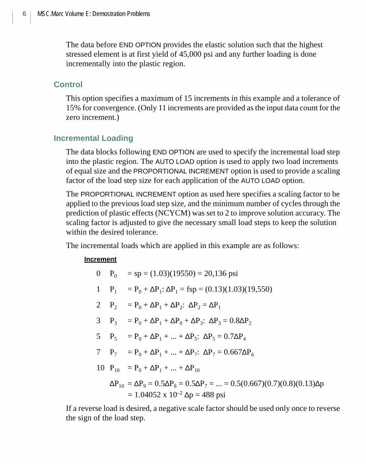
MSC.Marc Volume E: Demostration Problems
6
The data before END OPTION provides the elastic solution such that the highest stressed element is at first yield of 45,000 psi and any further loading is done incrementally into the plastic region.
Control
This option specifies a maximum of 15 increments in this example and a tolerance of 15% for convergence. (Only 11 increments are provided as the input data count for the zero increment.)
Incremental Loading
The data blocks following END OPTION are used to specify the incremental load step into the plastic region. The AUTO LOAD option is used to apply two load increments of equal size and the PROPORTIONAL INCREMENT option is used to provide a scaling factor of the load step size for each application of the AUTO LOAD option.
The PROPORTIONAL INCREMENT option as used here specifies a scaling factor to be applied to the previous load step size, and the minimum number of cycles through the prediction of plastic effects (NCYCM) was set to 2 to improve solution accuracy. The scaling factor is adjusted to give the necessary small load steps to keep the solution within the desired tolerance.
The incremental loads which are applied in this example are as follows:
Increment
0 P0 = sp = (1.03)(19550) = 20,136 psi
1 P1 = P0 + ∆P1: ∆P1 = fsp = (0.13)(1.03)(19,550)
2 P2 = P0 + ∆P1 + ∆P2: ∆P2 = ∆P1
3 P3 = P0 + ∆P1 + ∆P0 + ∆P3: ∆P3 = 0.8∆P2
5 P5 = P0 + ∆P1 + ... + ∆P5: ∆P5 = 0.7∆P4
7 P7 = P0 + ∆P1 + ... + ∆P7: ∆P7 = 0.667∆P6
10 P10 = P0 + ∆P1 + ... + ∆P10
∆P10 = ∆P9 = 0.5∆P8 = 0.5∆P7 = ... = 0.5(0.667)(0.7)(0.8)(0.13)∆p = 1.04052 x 10⁻² ∆p = 488 psi
If a reverse load is desired, a negative scale factor should be used only once to reverse the sign of the load step.
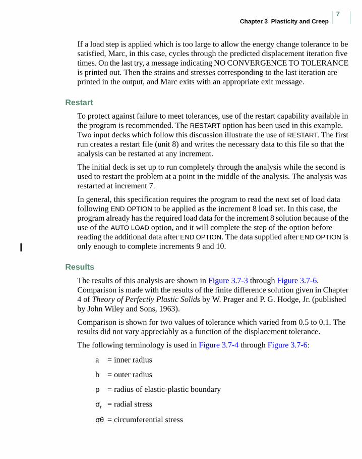
Chapter 3 Plasticity and Creep7
If a load step is applied which is too large to allow the energy change tolerance to be satisfied, Marc, in this case, cycles through the predicted displacement iteration five times. On the last try, a message indicating NO CONVERGENCE TO TOLERANCE is printed out. Then the strains and stresses corresponding to the last iteration are printed in the output, and Marc exits with an appropriate exit message.
Restart
To protect against failure to meet tolerances, use of the restart capability available in the program is recommended. The RESTART option has been used in this example. Two input decks which follow this discussion illustrate the use of RESTART. The first run creates a restart file (unit 8) and writes the necessary data to this file so that the analysis can be restarted at any increment.
The initial deck is set up to run completely through the analysis while the second is used to restart the problem at a point in the middle of the analysis. The analysis was restarted at increment 7.
In general, this specification requires the program to read the next set of load data following END OPTION to be applied as the increment 8 load set. In this case, the program already has the required load data for the increment 8 solution because of the use of the AUTO LOAD option, and it will complete the step of the option before reading the additional data after END OPTION. The data supplied after END OPTION is only enough to complete increments 9 and 10.
Results
The results of this analysis are shown in Figure 3.7-3 through Figure 3.7-6. Comparison is made with the results of the finite difference solution given in Chapter 4 of Theory of Perfectly Plastic Solids by W. Prager and P. G. Hodge, Jr. (published by John Wiley and Sons, 1963).
Comparison is shown for two values of tolerance which varied from 0.5 to 0.1. The results did not vary appreciably as a function of the displacement tolerance.
The following terminology is used in Figure 3.7-4 through Figure 3.7-6:
a = inner radius
b = outer radius
ρ = radius of elastic-plastic boundary
σr = radial stress
σθ = circumferential stress

MSC.Marc Volume E: Demostration Problems
8
σz = axial stress
Y = yield stress
k =
The elastic-plastic boundary is shown as a function of the pressure, p, in Figure 3.7-3.
For the plane strain condition, a numerical solution obtained by finite difference methods was given in the reference. The radial stress distribution for two different positions of the elastic-plastic boundary (ρ/a = 1.2 and ρ/a = 2.0) are compared to the solution given in the reference in Figure 3.7-4. Excellent agreement is observed. The circumferential stress distribution in the partially plastic tube is similarly compared in Figure 3.7-5. A comparison of the axial stress distribution is given in Figure 3.7-6. The two solutions are seen to be in good agreement.
Parameters, Options, and Subroutines Summary
Example e3x7a.dat:
Parameters Model Definition Options History Definition Options
END CONNECTIVITY AUTO LOAD
SCALE CONTROL CONTINUE
SIZING COORDINATES PROPORTIONAL INCREMENT
TITLE DIST LOADS
END OPTION
FIXED DISP
ISOTROPIC
PRINT CHOICE
RESTART
Y 3⁄

Chapter 3 Plasticity and Creep9
Example e3x7b.dat:
Figure 3.7-1 Cylinder Wall
Parameters Model Definition Options History Definition Options
END CONTROL AUTO LOAD
SCALE DIST LOADS CONTINUE
SIZING END OPTION PROPORTIONAL INCREMENT
TITLE FIXED DISP
ISOTROPIC
PRINT CHOICE
Symmetry Axis
Radial AxisR
Z
4 3
21
1”
1”
2”
p
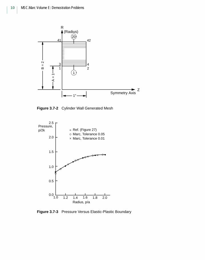
MSC.Marc Volume E: Demostration Problems
10
Figure 3.7-2 Cylinder Wall Generated Mesh
Figure 3.7-3 Pressure Versus Elastic-Plastic Boundary
Symmetry Axis
(Radius)R
42
43
1”
A =
1
B =
2
2041
121
Z
Ref. (Figure 27)Marc, Tolerance 0.05Marc, Tolerance 0.01
Pressure,p/2k
2.5
2.0
1.5
1.0
0.5
0.01.0 1.2 1.4 1.6 1.8 2.0
Radius, p/a
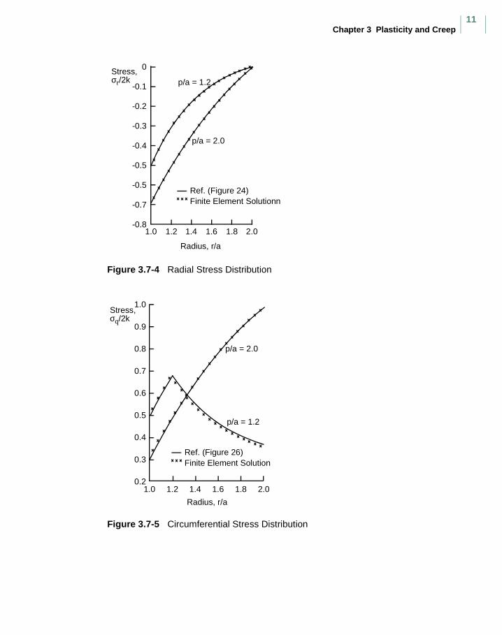
Chapter 3 Plasticity and Creep11
Figure 3.7-4 Radial Stress Distribution
Figure 3.7-5 Circumferential Stress Distribution
Ref. (Figure 24)Finite Element Solutionn
Stress,σr/2k
0
-0.1
-0.2
-0.4
-0.5
-0.81.0 1.2 1.4 1.6 1.8 2.0
Radius, r/a
-0.3
-0.5
-0.7
p/a = 1.2
p/a = 2.0
Ref. (Figure 26)Finite Element Solution
Stress,σq/2k
1.0
0.9
0.8
0.6
0.4
0.21.0 1.2 1.4 1.6 1.8 2.0
Radius, r/a
0.7
0.5
0.3
p/a = 1.2
p/a = 2.0
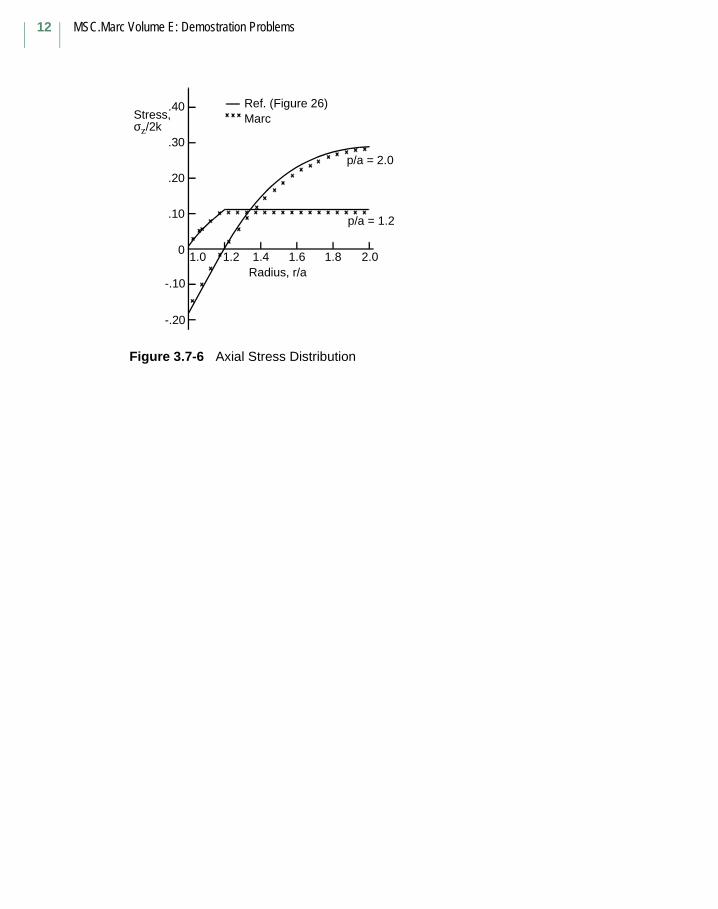
MSC.Marc Volume E: Demostration Problems
12
Figure 3.7-6 Axial Stress Distribution
Ref. (Figure 26)MarcStress,
σz/2k
.40
.30
.20
-.10
1.0 1.2 1.4 1.6 1.8 2.0Radius, r/a
.10
0
p/a = 1.2
p/a = 2.0
-.20
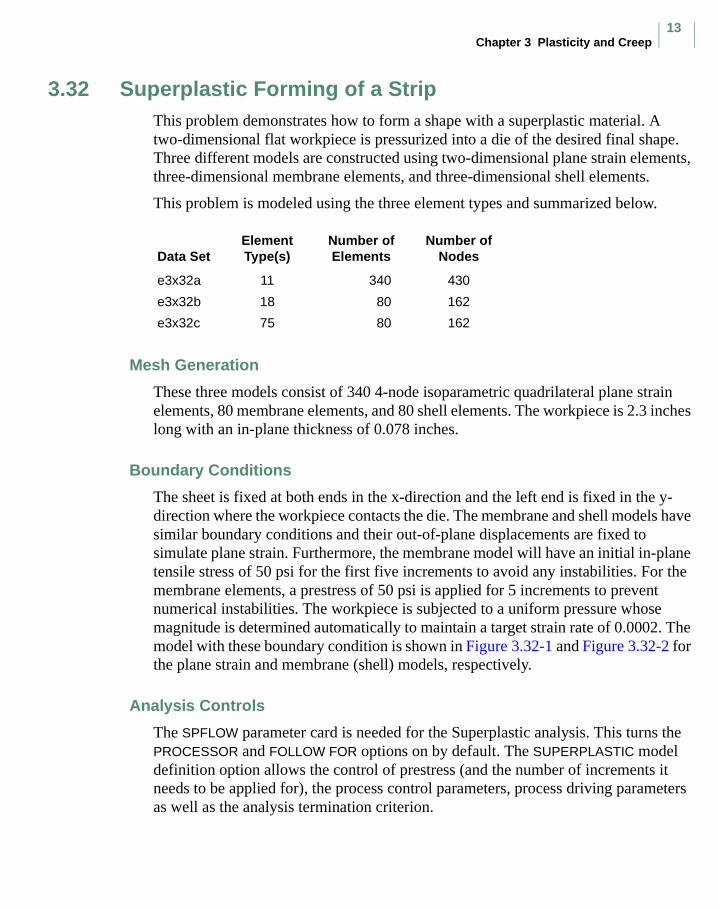
Chapter 3 Plasticity and Creep13
3.32 Superplastic Forming of a StripThis problem demonstrates how to form a shape with a superplastic material. A two-dimensional flat workpiece is pressurized into a die of the desired final shape. Three different models are constructed using two-dimensional plane strain elements, three-dimensional membrane elements, and three-dimensional shell elements.
This problem is modeled using the three element types and summarized below.
Mesh Generation
These three models consist of 340 4-node isoparametric quadrilateral plane strain elements, 80 membrane elements, and 80 shell elements. The workpiece is 2.3 inches long with an in-plane thickness of 0.078 inches.
Boundary Conditions
The sheet is fixed at both ends in the x-direction and the left end is fixed in the y-direction where the workpiece contacts the die. The membrane and shell models have similar boundary conditions and their out-of-plane displacements are fixed to simulate plane strain. Furthermore, the membrane model will have an initial in-plane tensile stress of 50 psi for the first five increments to avoid any instabilities. For the membrane elements, a prestress of 50 psi is applied for 5 increments to prevent numerical instabilities. The workpiece is subjected to a uniform pressure whose magnitude is determined automatically to maintain a target strain rate of 0.0002. The model with these boundary condition is shown in Figure 3.32-1 and Figure 3.32-2 for the plane strain and membrane (shell) models, respectively.
Analysis Controls
The SPFLOW parameter card is needed for the Superplastic analysis. This turns the PROCESSOR and FOLLOW FOR options on by default. The SUPERPLASTIC model definition option allows the control of prestress (and the number of increments it needs to be applied for), the process control parameters, process driving parameters as well as the analysis termination criterion.
Data SetElement Type(s)
Number of Elements
Number of Nodes
e3x32a 11 340 430
e3x32b 18 80 162
e3x32c 75 80 162
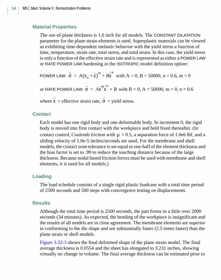
MSC.Marc Volume E: Demostration Problems
14
Material Properties
The out-of-plane thickness is 1.0 inch for all models. The CONSTANT DILATATION parameter for the plane strain elements is used. Superplastic materials can be viewed as exhibiting time-dependent inelastic behavior with the yield stress a function of time, temperature, strain rate, total stress, and total strain. In this case, the yield stress is only a function of the effective strain rate and is represented as either a POWER LAW or RATE POWER LAW hardening in the ISOTROPIC model definition option:
POWER LAW: with A = 0, B = 50000, n = 0.6, m = 0
or RATE POWER LAW: with B = 0, A = 50000, m = 0, n = 0.6
where = effective strain rate, = yield stress.
Contact
Each model has one rigid body and one deformable body. In increment 0, the rigid body is moved into first contact with the workpiece and held fixed thereafter. (In contact control, Coulomb friction with = 0.5, a separation force of 1.0e6 lbf, and a sliding velocity of 1.0e-5 inches/seconds are used. For the membrane and shell models, the contact zone tolerance is set equal to one-half of the element thickness and the bias factor is set to .99 to reduce the touching distance because of the large thickness. Because nodal based friction forces must be used with membrane and shell elements, it is used for all models.)
Loading
The load schedule consists of a single rigid plastic loadcase with a total time period of 2500 seconds and 500 steps with convergence testing on displacements.
Results
Although the total time period is 2500 seconds, the part forms in a little over 2000 seconds (34 minutes). As expected, the bending of the workpiece is insignificant and the results of all models are in close agreement. The membrane elements are superior in conforming to the die shape and are substantially faster (2.5 times faster) than the plane strain or shell models.
Figure 3.32-3 shows the final deformed shape of the plane strain model. The final average thickness is 0.0554 and the sheet has elongated to 3.231 inches, showing virtually no change in volume. The final average thickness can be estimated prior to
σ A εo ε+( )mBε
· n+=
σ Aεmε· n
B+=
ε·
σ
µ
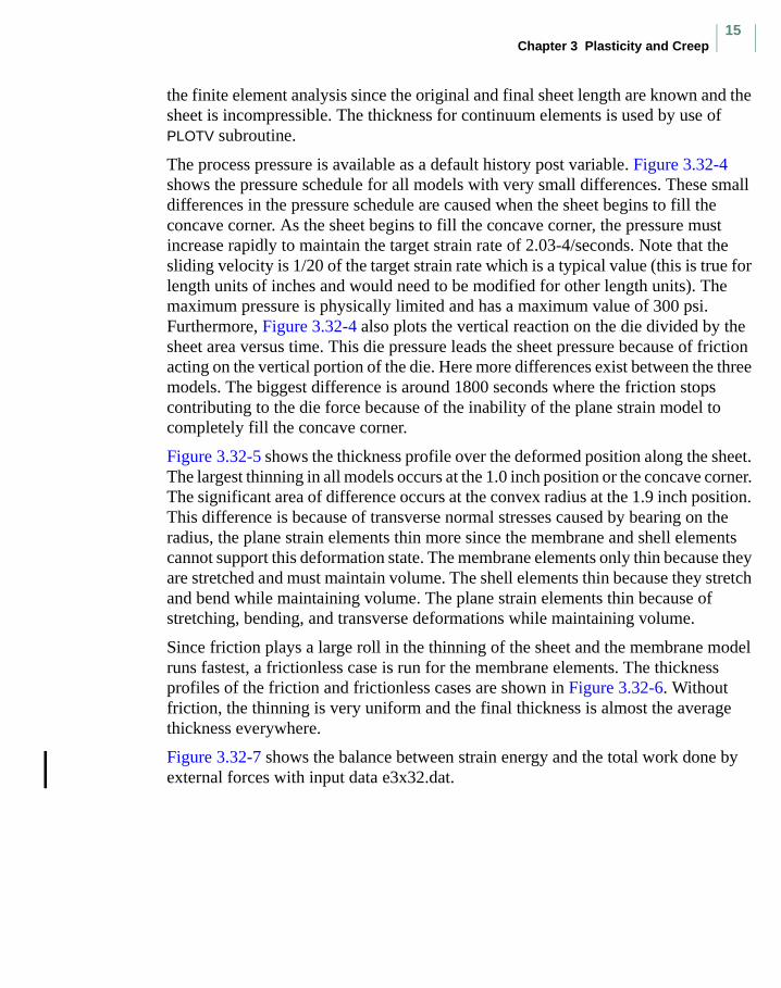
Chapter 3 Plasticity and Creep15
the finite element analysis since the original and final sheet length are known and the sheet is incompressible. The thickness for continuum elements is used by use of PLOTV subroutine.
The process pressure is available as a default history post variable. Figure 3.32-4 shows the pressure schedule for all models with very small differences. These small differences in the pressure schedule are caused when the sheet begins to fill the concave corner. As the sheet begins to fill the concave corner, the pressure must increase rapidly to maintain the target strain rate of 2.03-4/seconds. Note that the sliding velocity is 1/20 of the target strain rate which is a typical value (this is true for length units of inches and would need to be modified for other length units). The maximum pressure is physically limited and has a maximum value of 300 psi. Furthermore, Figure 3.32-4 also plots the vertical reaction on the die divided by the sheet area versus time. This die pressure leads the sheet pressure because of friction acting on the vertical portion of the die. Here more differences exist between the three models. The biggest difference is around 1800 seconds where the friction stops contributing to the die force because of the inability of the plane strain model to completely fill the concave corner.
Figure 3.32-5 shows the thickness profile over the deformed position along the sheet. The largest thinning in all models occurs at the 1.0 inch position or the concave corner. The significant area of difference occurs at the convex radius at the 1.9 inch position. This difference is because of transverse normal stresses caused by bearing on the radius, the plane strain elements thin more since the membrane and shell elements cannot support this deformation state. The membrane elements only thin because they are stretched and must maintain volume. The shell elements thin because they stretch and bend while maintaining volume. The plane strain elements thin because of stretching, bending, and transverse deformations while maintaining volume.
Since friction plays a large roll in the thinning of the sheet and the membrane model runs fastest, a frictionless case is run for the membrane elements. The thickness profiles of the friction and frictionless cases are shown in Figure 3.32-6. Without friction, the thinning is very uniform and the final thickness is almost the average thickness everywhere.
Figure 3.32-7 shows the balance between strain energy and the total work done by external forces with input data e3x32.dat.

MSC.Marc Volume E: Demostration Problems
16
Summary of Parameters, Options, and Subroutines Used
Example e3x32a.dat, e3x32b, e3x32c:
Parameters Model Definition Options History Definition Options
ELEMENTS CONNECTIVITY AUTO LOAD
END CONTROL CONTINUE
PRINT COORDINATES DIST LOADS
SIZING DIST LOADS MOTION CHANGE
SPFLOW FIXED DISP SUPERPLASTIC
TITLE GEOMETRY TIME STEP
ISOTROPIC
NO PRINT
OPTIMIZE
POST
SOLVER
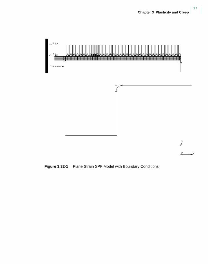
Chapter 3 Plasticity and Creep17
Figure 3.32-1 Plane Strain SPF Model with Boundary Conditions
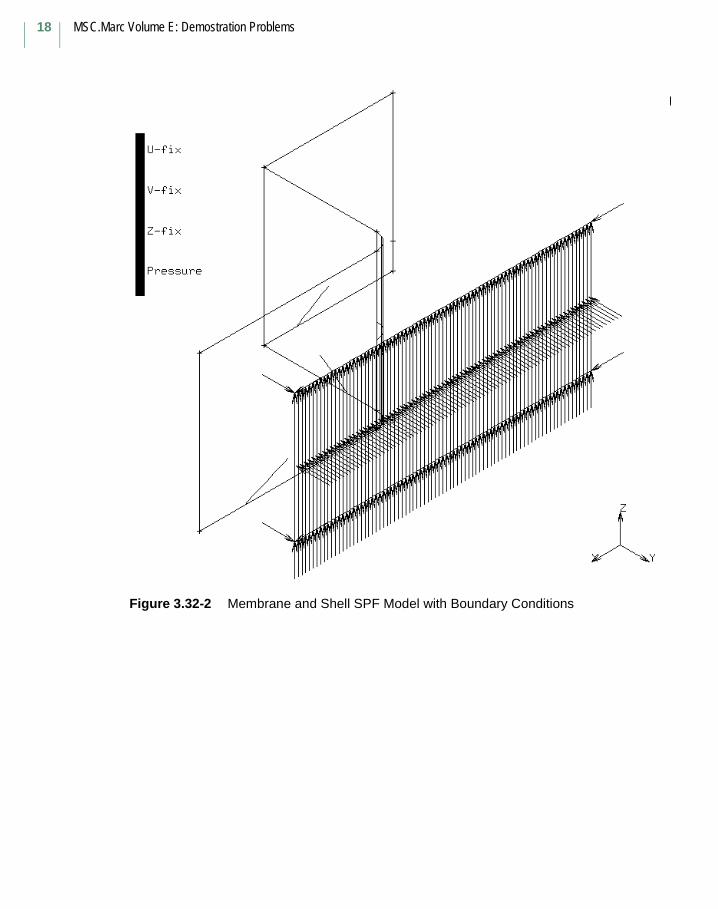
MSC.Marc Volume E: Demostration Problems
18
Figure 3.32-2 Membrane and Shell SPF Model with Boundary Conditions
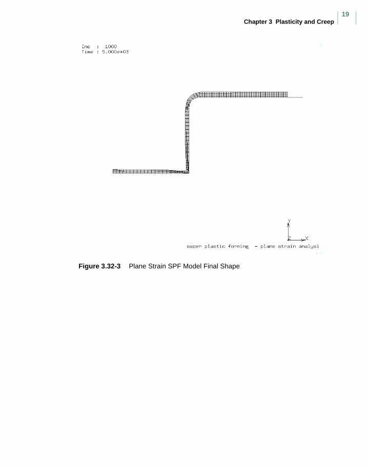
Chapter 3 Plasticity and Creep19
Figure 3.32-3 Plane Strain SPF Model Final Shape
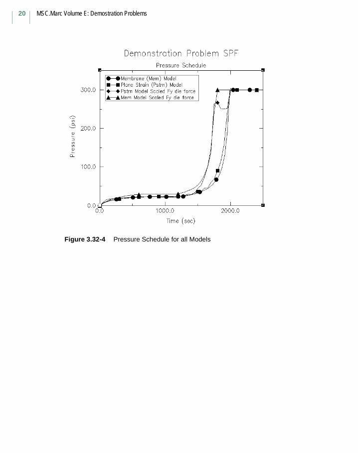
MSC.Marc Volume E: Demostration Problems
20
Figure 3.32-4 Pressure Schedule for all Models
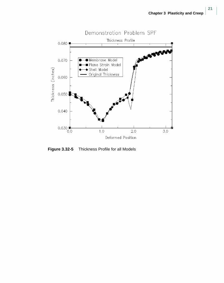
Chapter 3 Plasticity and Creep21
Figure 3.32-5 Thickness Profile for all Models
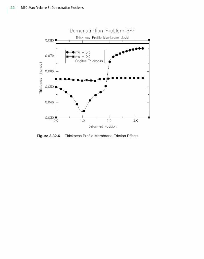
MSC.Marc Volume E: Demostration Problems
22
Figure 3.32-6 Thickness Profile Membrane Friction Effects
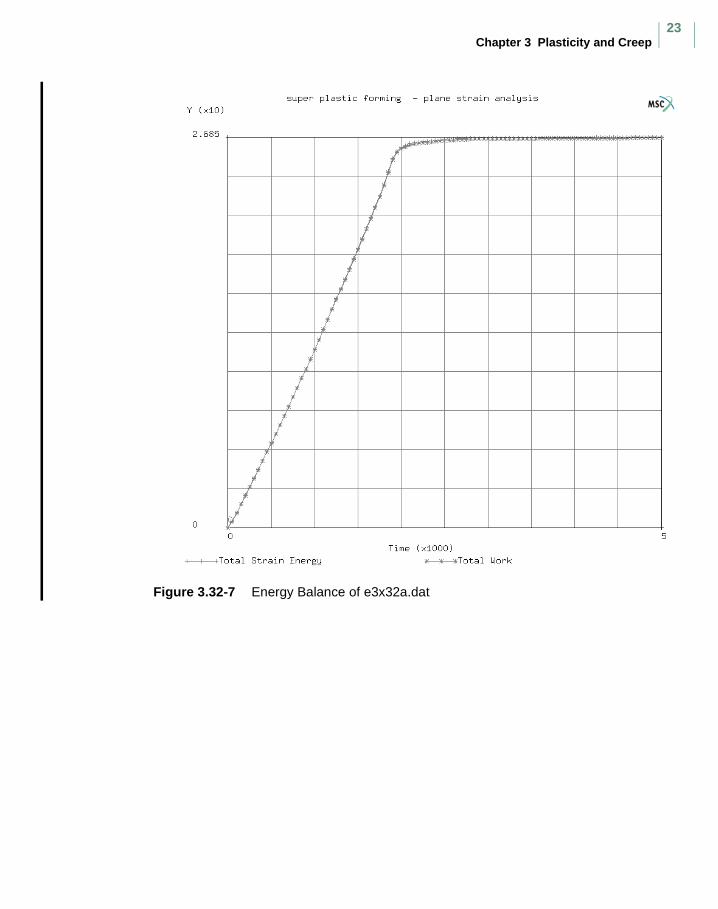
Chapter 3 Plasticity and Creep23
Figure 3.32-7 Energy Balance of e3x32a.dat
MSC.Marc Volume E: Demostration Problems
24
3.33 Large Strain Tensile Loading of a Plate with a HoleThis problem simulates the tensile loading of a plate with a hole to large strains. The
example demonstrates the accuracy of the finite strain plasticity algorithm using FeFp formulation to simulate large strains. The multiplicative decomposition procedure is invoked using the PLASTICITY option.
This problem is modeled using two techniques summarized below.
Element
This problem simulates two-dimensional plane stress and plane strain cases. For the plane stress case, an 8-node plane stress isoparametric element type 26 is used to construct a mesh while for the plane strain case, an 8-node plane stress isoparametric element type 27 is used. There are two degrees of freedom per node with a bi-quadratic interpolation and eight-point Gaussian quadrature for stiffness assembly.
Model
Due to symmetry of the geometry and loading, a quarter of the actual model is simulated. The finite element model is made up of 20 elements and 79 nodes. There is a total of 158 degrees of freedom. The model is shown in Figure 3.33-1.
Geometry
The model is assumed to be a square of side five units from which a quarter of a circle of radius one unit has been cut out. In the plane stress case, the initial thickness is one unit.
Material Properties
The material is assumed to be isotropic elastic plastic. The Young’s modulus is 3.0E+07 psi. Poisson’s ratio is 0.30. The initial yield stress is 5.0E+04 psi. The hardening behavior is given in Table 3.33-1.
Data SetElement Type(s)
Number of Elements
Number of Nodes
Differentiating Features
e3x33 26 20 79 Plane Stress
e3x33b 27 20 79 Plane Strain
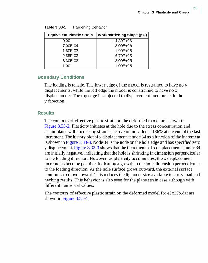
Chapter 3 Plasticity and Creep25
Boundary Conditions
The loading is tensile. The lower edge of the model is restrained to have no y displacements, while the left edge the model is constrained to have no x displacements. The top edge is subjected to displacement increments in the y direction.
Results
The contours of effective plastic strain on the deformed model are shown in Figure 3.33-2. Plasticity initiates at the hole due to the stress concentration and accumulates with increasing strain. The maximum value is 186% at the end of the last increment. The history plot of x displacement at node 34 as a function of the increment is shown in Figure 3.33-3. Node 34 is the node on the hole edge and has specified zero y displacement. Figure 3.33-3 shows that the increments of x displacement at node 34 are initially negative, indicating that the hole is shrinking in dimension perpendicular to the loading direction. However, as plasticity accumulates, the x displacement increments become positive, indicating a growth in the hole dimension perpendicular to the loading direction. As the hole surface grows outward, the external surface continues to move inward. This reduces the ligament size available to carry load and necking results. This behavior is also seen for the plane strain case although with different numerical values.
The contours of effective plastic strain on the deformed model for e3x33b.dat are shown in Figure 3.33-4.
Table 3.33-1 Hardening Behavior
Equivalent Plastic Strain Workhardening Slope (psi)
0.00 14.30E+067.00E-04 3.00E+061.60E-03 1.90E+062.55E-03 6.70E+053.30E-03 3.00E+051.00 1.00E+05
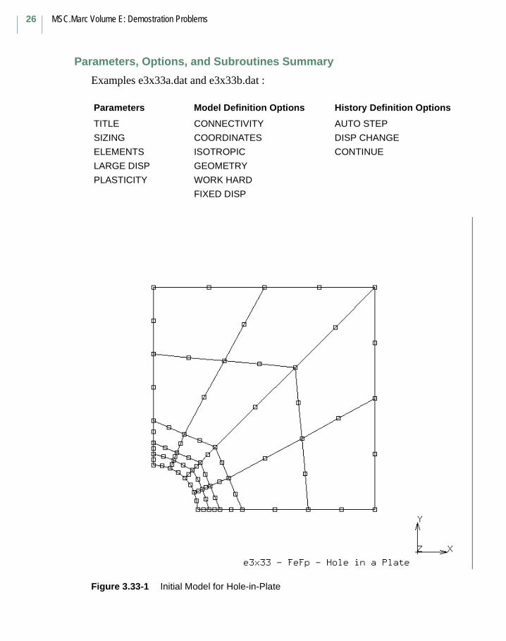
MSC.Marc Volume E: Demostration Problems
26
Parameters, Options, and Subroutines Summary
Examples e3x33a.dat and e3x33b.dat :
Figure 3.33-1 Initial Model for Hole-in-Plate
Parameters Model Definition Options History Definition Options
TITLE CONNECTIVITY AUTO STEP
SIZING COORDINATES DISP CHANGE
ELEMENTS ISOTROPIC CONTINUE
LARGE DISP GEOMETRY
PLASTICITY WORK HARD
FIXED DISP
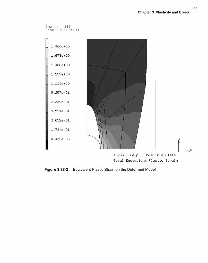
Chapter 3 Plasticity and Creep27
Figure 3.33-2 Equivalent Plastic Strain on the Deformed Model
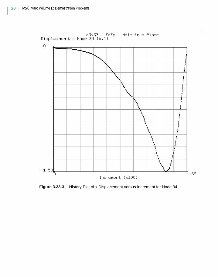
MSC.Marc Volume E: Demostration Problems
28
Figure 3.33-3 History Plot of x Displacement versus Increment for Node 34
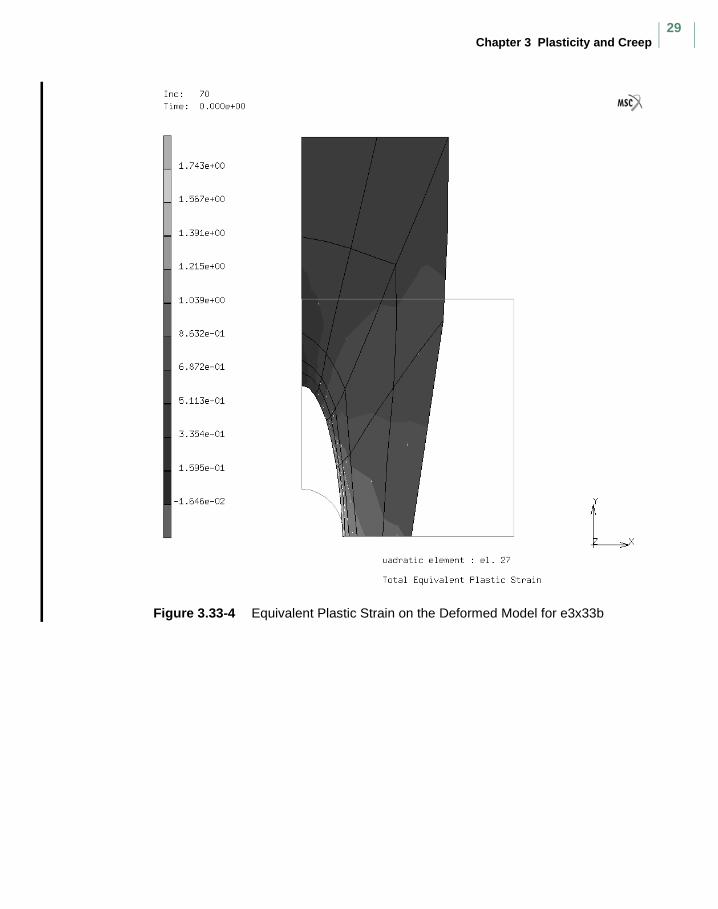
Chapter 3 Plasticity and Creep29
Figure 3.33-4 Equivalent Plastic Strain on the Deformed Model for e3x33b

MSC.Marc Volume E: Demostration Problems
30
Volume E: Demonstration
Problems, Part III

Volume E: Demonstration Problems, Part III31

MSC.Marc Volume E: Demostration Problems
32
Chapter 5 Heat Transfer

Chapter 5 Heat Transfer33
MSC.Marc Volume E: Demostration Problems
34
5.17 Cooling of Electronic ChipsThis problem demonstrates the air cooling of an electronic chip at room temperature. The comparison of the no-inclusion of heat convection, e5x17a.dat, and the inclusion of the contribution of heat convection, e5x17b.dat, by air is made. The nonsymmetric solver is turned on automatically when heat convection is included.
This problem is modeled using the two techniques summarized below.
Element
Element type 39 is used for both the air region and the chip body. The model is shown in Figures 5.17-1 and 5.17-3.
Material properties
Room temperature thermal properties for air are used. The specific heat is 1.0057 kJ/kg.°C, the density is 1.177e-6 kg/cm3, and thermal conductivity is 0.0002624 W/cm.°C. Thermal properties for pure copper are used for the chip. The specific heat is 0.3855 kJ/kg.°C, the density is 8.893e-3 kg/cm3, and thermal conductivity is 3.8015 W/cm.°C. Assume the variation of properties with temperature is negligible.
Initial Conditions
The initial nodal temperature for chips is 40°C and for air is 10°C throughout.
Boundary Conditions
The temperature of the air far away from chips is fixed at 10°C and velocity of the air is kept at a constant 1400 cm/second. The velocity of the chips is zero.
Transient Nonauto
A fixed time step is used to simulate the cooling process near steady-state condition.
Data SetElement Type(s)
Number of Elements
Number of Nodes
Differentiating Features
e5x17a 39 360 399 Exclude convection
e5x17b 39 360 399 Include convection
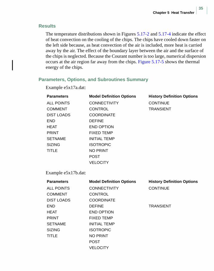
Chapter 5 Heat Transfer35
Results
The temperature distributions shown in Figures 5.17-2 and 5.17-4 indicate the effect of heat convection on the cooling of the chips. The chips have cooled down faster on the left side because, as heat convection of the air is included, more heat is carried away by the air. The effect of the boundary layer between the air and the surface of the chips is neglected. Because the Courant number is too large, numerical dispersion occurs at the air region far away from the chips. Figure 5.17-5 shows the thermal energy of the chips.
Parameters, Options, and Subroutines Summary
Example e5x17a.dat:
Example e5x17b.dat:
Parameters Model Definition Options History Definition Options
ALL POINTS CONNECTIVITY CONTINUE
COMMENT CONTROL TRANSIENT
DIST LOADS COORDINATE
END DEFINE
HEAT END OPTION
PRINT FIXED TEMP
SETNAME INITIAL TEMP
SIZING ISOTROPIC
TITLE NO PRINT
POST
VELOCITY
Parameters Model Definition Options History Definition Options
ALL POINTS CONNECTIVITY CONTINUE
COMMENT CONTROL
DIST LOADS COORDINATE
END DEFINE TRANSIENT
HEAT END OPTION
PRINT FIXED TEMP
SETNAME INITIAL TEMP
SIZING ISOTROPIC
TITLE NO PRINT
POST
VELOCITY
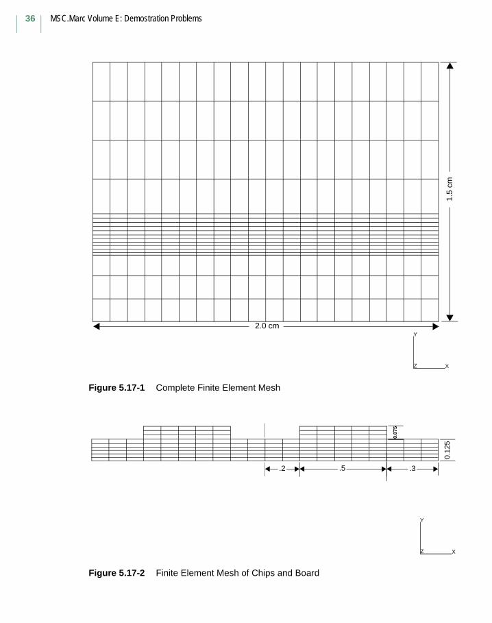
MSC.Marc Volume E: Demostration Problems
36
Figure 5.17-1 Complete Finite Element Mesh
Figure 5.17-2 Finite Element Mesh of Chips and Board
2.0 cm
1.5
cm
Y
Z X
0.12
5
0.07
5
.2 .5 .3
Y
Z X
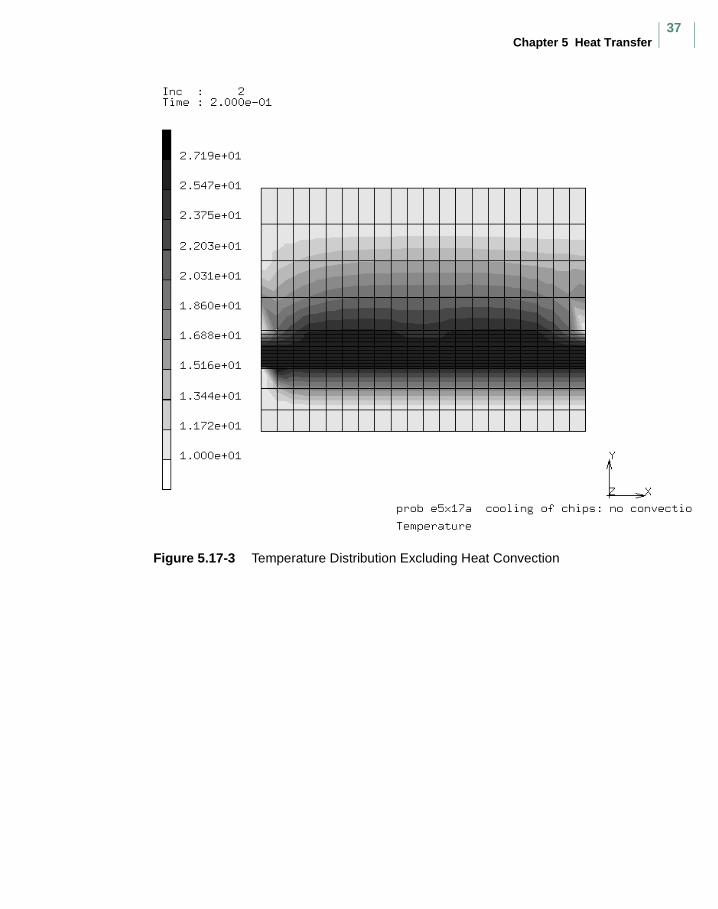
Chapter 5 Heat Transfer37
Figure 5.17-3 Temperature Distribution Excluding Heat Convection
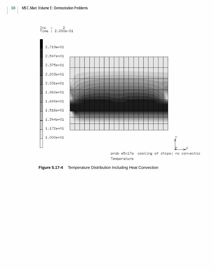
MSC.Marc Volume E: Demostration Problems
38
Figure 5.17-4 Temperature Distribution Including Heat Convection
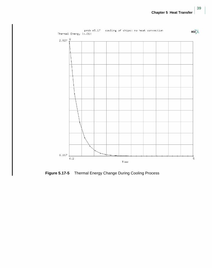
Chapter 5 Heat Transfer39
Figure 5.17-5 Thermal Energy Change During Cooling Process

MSC.Marc Volume E: Demostration Problems
40
Chapter 6 Dynamics

Chapter 6 Dynamics41
MSC.Marc Volume E: Demostration Problems
42
6.22 Dynamic Collapse of a CylinderIn this example, the dynamic collapse of a cylinder is analyzed. The cylinder, with a radius of 0.02 m, a wall thickness of 0.00131 m and a length of 0.08 m, is compressed between two rigid bodies, of which one is fixed and one has a velocity of 50 m/s.
Element
Element type 10, a four-node axisymmetric isoparametric element with full integration is used to model the cylinder.
Constant Dilatation
The CONSTANT DILATATION parameter is used since large plastic deformations occur. In this way, the incompressibility of the material during plastic deformations can be accounted for without showing a too stiff behavior.
Dynamic
The Single Step Houbolt dynamic time integration method is activated using the DYNAMIC parameter. This method is especially recommended for dynamic contact problems, since is possesses high-frequency dissipation, so that undesired, numerically triggered, high-frequency oscillations may be damped out quickly.
Lump
The mass matrices are applied in a lumped form using the LUMP parameter.
Plasticity
The material behavior is based on small strain elasticity and large strain plasticity based on the additive decomposition of the strain tensor.
Isotropic
The elastic material properties are given by a Young’s modulus of 1 x 10¹¹ N/mm2, a
Poisson’s ratio of 0.3 and a density of 7000 kg/mm3. Plasticity is according to the von
Mises criterion with an initial yield stress of 1 x 10⁸ N/mm2.
Work Hard,Data
A linear hardening modulus of 3 x 10 N/m2 is defined using the WORK HARD,DATA model definition option.
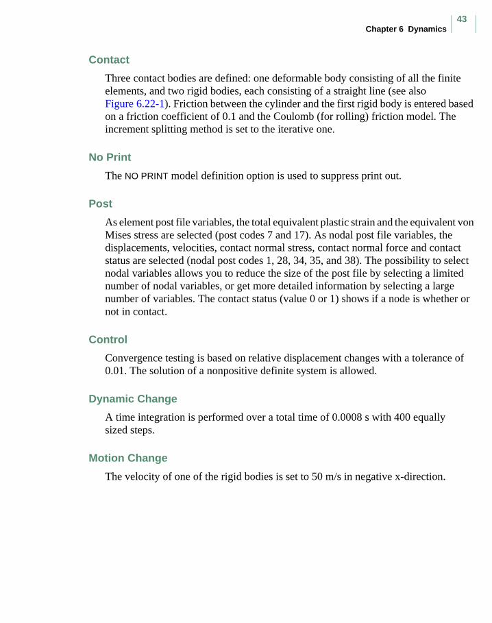
Chapter 6 Dynamics43
Contact
Three contact bodies are defined: one deformable body consisting of all the finite elements, and two rigid bodies, each consisting of a straight line (see also Figure 6.22-1). Friction between the cylinder and the first rigid body is entered based on a friction coefficient of 0.1 and the Coulomb (for rolling) friction model. The increment splitting method is set to the iterative one.
No Print
The NO PRINT model definition option is used to suppress print out.
Post
As element post file variables, the total equivalent plastic strain and the equivalent von Mises stress are selected (post codes 7 and 17). As nodal post file variables, the displacements, velocities, contact normal stress, contact normal force and contact status are selected (nodal post codes 1, 28, 34, 35, and 38). The possibility to select nodal variables allows you to reduce the size of the post file by selecting a limited number of nodal variables, or get more detailed information by selecting a large number of variables. The contact status (value 0 or 1) shows if a node is whether or not in contact.
Control
Convergence testing is based on relative displacement changes with a tolerance of 0.01. The solution of a nonpositive definite system is allowed.
Dynamic Change
A time integration is performed over a total time of 0.0008 s with 400 equally sized steps.
Motion Change
The velocity of one of the rigid bodies is set to 50 m/s in negative x-direction.
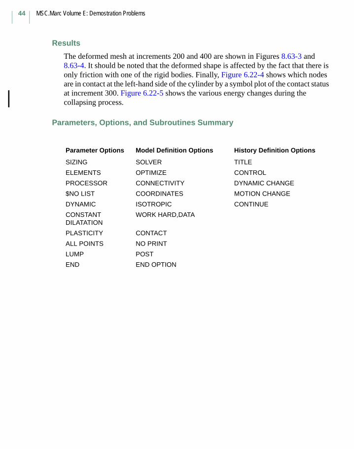
MSC.Marc Volume E: Demostration Problems
44
Results
The deformed mesh at increments 200 and 400 are shown in Figures 8.63-3 and 8.63-4. It should be noted that the deformed shape is affected by the fact that there is only friction with one of the rigid bodies. Finally, Figure 6.22-4 shows which nodes are in contact at the left-hand side of the cylinder by a symbol plot of the contact status at increment 300. Figure 6.22-5 shows the various energy changes during the collapsing process.
Parameters, Options, and Subroutines Summary
Parameter Options Model Definition Options History Definition Options
SIZING SOLVER TITLE
ELEMENTS OPTIMIZE CONTROL
PROCESSOR CONNECTIVITY DYNAMIC CHANGE
$NO LIST COORDINATES MOTION CHANGE
DYNAMIC ISOTROPIC CONTINUE
CONSTANT DILATATION
WORK HARD,DATA
PLASTICITY CONTACT
ALL POINTS NO PRINT
LUMP POST
END END OPTION
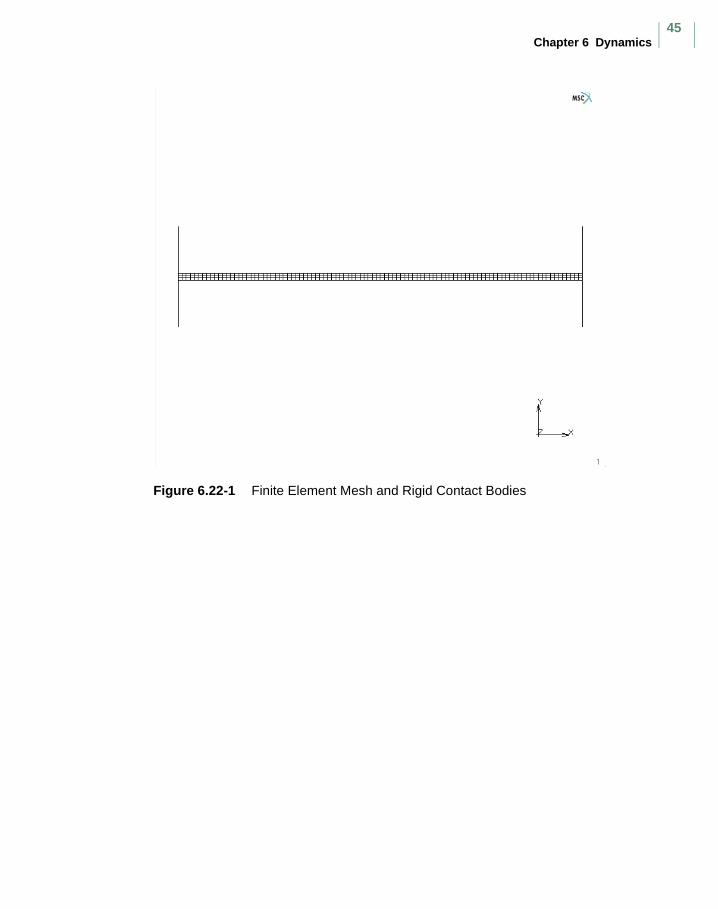
Chapter 6 Dynamics45
Figure 6.22-1 Finite Element Mesh and Rigid Contact Bodies
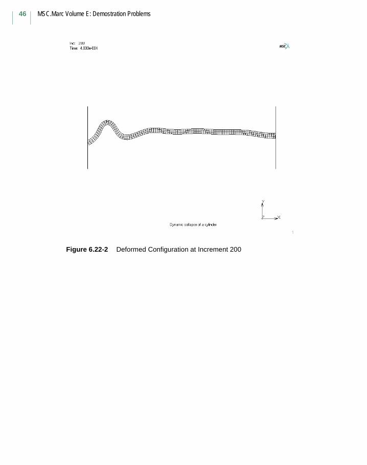
MSC.Marc Volume E: Demostration Problems
46
Figure 6.22-2 Deformed Configuration at Increment 200
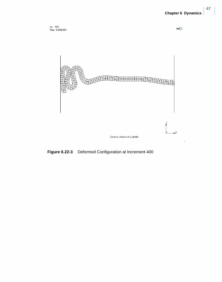
Chapter 6 Dynamics47
Figure 6.22-3 Deformed Configuration at Increment 400
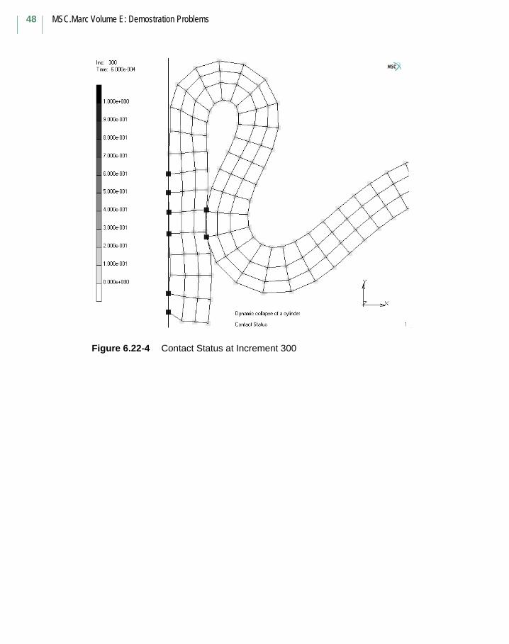
MSC.Marc Volume E: Demostration Problems
48
Figure 6.22-4 Contact Status at Increment 300
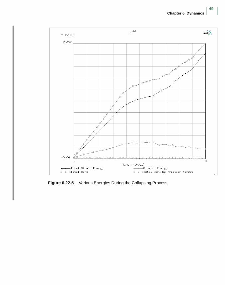
Chapter 6 Dynamics49
Figure 6.22-5 Various Energies During the Collapsing Process

MSC.Marc Volume E: Demostration Problems
50
Volume E: Demonstration
Problems, Part IV

Volume E: Demonstration Problems, Part IV51

MSC.Marc Volume E: Demostration Problems
52
Chapter 7 Contact

Chapter 7 Contact53
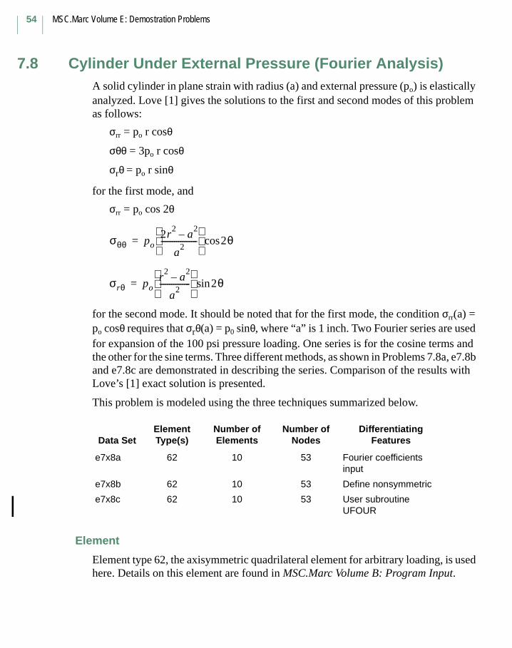
MSC.Marc Volume E: Demostration Problems
54
7.8 Cylinder Under External Pressure (Fourier Analysis)A solid cylinder in plane strain with radius (a) and external pressure (po) is elastically analyzed. Love [1] gives the solutions to the first and second modes of this problem as follows:
σrr = po r cosθ
σθθ = 3po r cosθ
σrθ = po r sinθ
for the first mode, and
σrr = po cos 2θ
for the second mode. It should be noted that for the first mode, the condition σrr(a) = po cosθ requires that σrθ(a) = p0 sinθ, where “a” is 1 inch. Two Fourier series are used for expansion of the 100 psi pressure loading. One series is for the cosine terms and the other for the sine terms. Three different methods, as shown in Problems 7.8a, e7.8b and e7.8c are demonstrated in describing the series. Comparison of the results with Love’s [1] exact solution is presented.
This problem is modeled using the three techniques summarized below.
Element
Element type 62, the axisymmetric quadrilateral element for arbitrary loading, is used here. Details on this element are found in MSC.Marc Volume B: Program Input.
Data SetElement Type(s)
Number of Elements
Number of Nodes
Differentiating Features
e7x8a 62 10 53 Fourier coefficients input
e7x8b 62 10 53 Define nonsymmetric
e7x8c 62 10 53 User subroutine UFOUR
σθθ po2r
2a
2–
a2
-------------------
2θcos=
σrθ por
2a
2–
a2
----------------
2θsin=

Chapter 7 Contact55
Model
The geometry and mesh used are shown in Figure 7.8-1. The solid cylinder has a height of 0.1 inch and a radius of 1.0 inch. The mesh has 10 elements and 53 nodes.
Geometry
This option is not required for this problem.
Material Properties
The elastic material data assumed for this example is Young’s modulus (E) is 30. x 106 psi and Poisson’s ratio (ν) is 0.25.
Loading
The 100 psi external pressure is specified as a distributed load (IBODY=0) and associated with Fourier series number 1. The -100 psi shear is specified as a uniform load in the circumferential direction (IBODY=14) and associated with Fourier series number 2. Only element 10 is specified with the above loads using the DIST LOAD option.
Boundary Conditions
All nodes on the plane Z = 0. and Z = 0.1 are constrained in the axial direction such that only radial motion is permitted. Nodes 1, 2, and 3 on the plane R = 0 are also constrained in the radial direction due to symmetry.
Fourier
Three different ways are used to describe the series:
1. Specify the first two nonzero terms for series number 1 by evaluating the following integral:
and the first nonzero term for series number 2 by evaluating the following integral:
an1π---
θcos2θcos
nθ dθcoso
2π∫ 1 n, 1 and 2,=0 all n except,
= =
bn1π--- θ nθ dθsinsin
o
2π∫ 1 n, 1=0 all n except,
= =
MSC.Marc Volume E: Demostration Problems
56
2. Describe the function F(θ) which is to be expanded into a Fourier series by an arbitrary number (say 5) of [θ, F(θ)] pairs of data.
3. Use user subroutine UFOUR to generate an arbitrary number of [θ,F(θ)] pairs and let Marc calculate the Fourier series coefficients. Five pairs of [θ,F(θ)] are defined in this example.
It should be pointed out that five pairs of [θ,F(θ)] have been chosen for demonstration only. It is easy to add more by changing the number 5 in the user subroutine UFOUR. An increased number of [θ,F(θ)] pairs would yield better results in comparison with the exact coefficient evaluations.
Results
The results for the radial and circumferential stresses of Problem e7.8a and Love’s exact solution are plotted in Figure 7.8-2 and Figure 7.8-3. They indicate that the finite element solutions are in good agreement with the exact solutions.
Reference
Love, A.E.H., A Treatise on the Mathematical Theory of Elasticity, Dover, New York.
Parameters, Options, and Subroutines Summary
Example e7x8a.dat:
Parameters Model Definition Options
ELEMENT CONNECTIVITY
END CONTROL
FOURIER COORDINATE
SIZING DIST LOADS
TITLE END OPTION
FIXED DISP
FOURIER
ISOTROPIC
RESTART

Chapter 7 Contact57
Example e7x8b.dat:
Example e7x8c.dat:
User subroutine in u7x8c.f: UFOUR
Parameters Model Definition Options
ELEMENT CONNECTIVITY
END CONTROL
FOURIER COORDINATE
SIZING DIST LOADS
TITLE END OPTION
FIXED DISP
FOURIER
ISOTROPIC
RESTART
Parameters Model Definition Options
ELEMENT CONNECTIVITY
END CONTROL
FOURIER COORDINATE
SIZING DIST LOADS
TITLE END OPTION
FIXED DISP
FOURIER
ISOTROPIC
RESTART
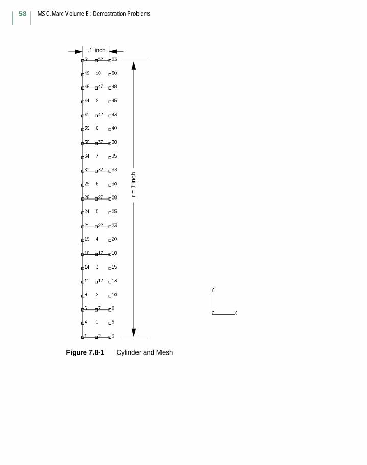
MSC.Marc Volume E: Demostration Problems
58
Figure 7.8-1 Cylinder and Mesh
r =
1 in
ch
.1 inch
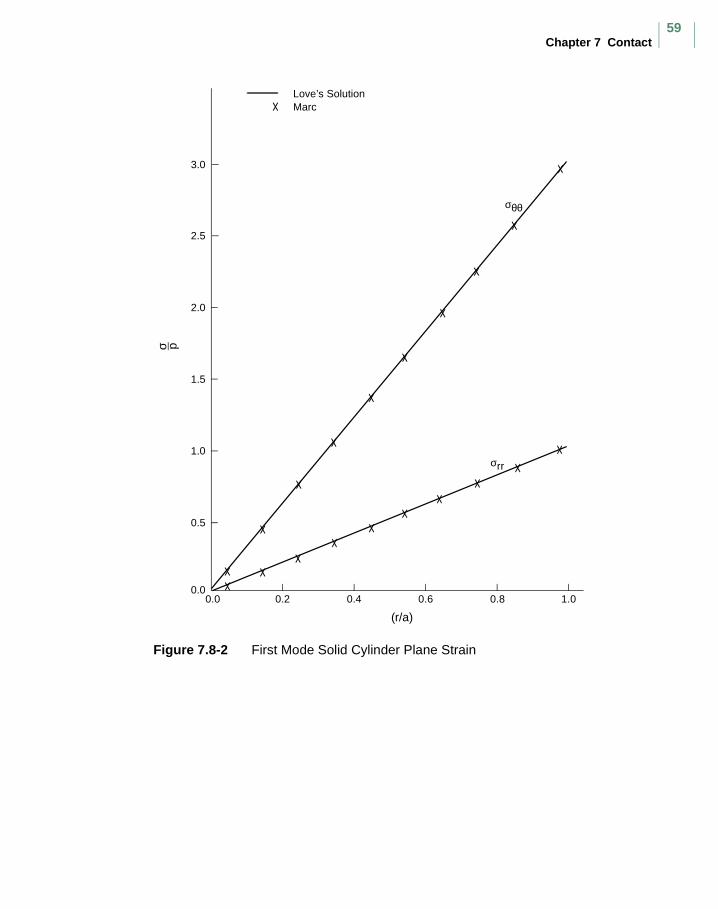
Chapter 7 Contact59
Figure 7.8-2 First Mode Solid Cylinder Plane Strain
Love’s SolutionMarc
σrr
2.0
1.5
1.0
0.5
0.00.0 0.2 0.4
(r/a)
0.6 0.8 1.0
σθθ
2.5
3.0σ p
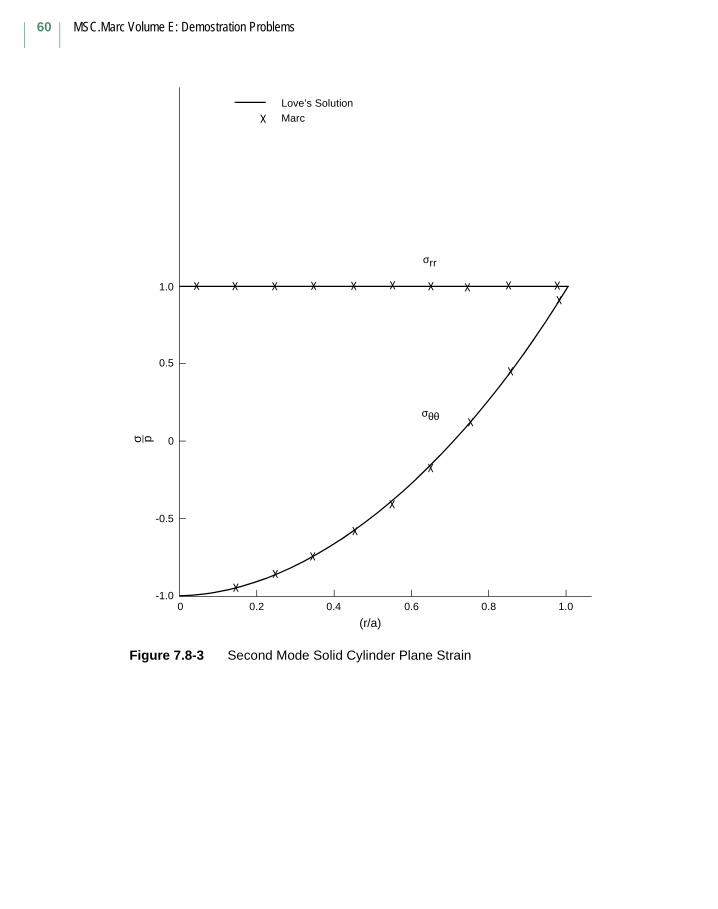
MSC.Marc Volume E: Demostration Problems
60
Figure 7.8-3 Second Mode Solid Cylinder Plane Strain
Love’s SolutionMarc
σrr
1.0
0.5
0
-0.5
-1.00 0.2 0.4
(r/a)0.6 0.8 1.0
σ p
σθθ
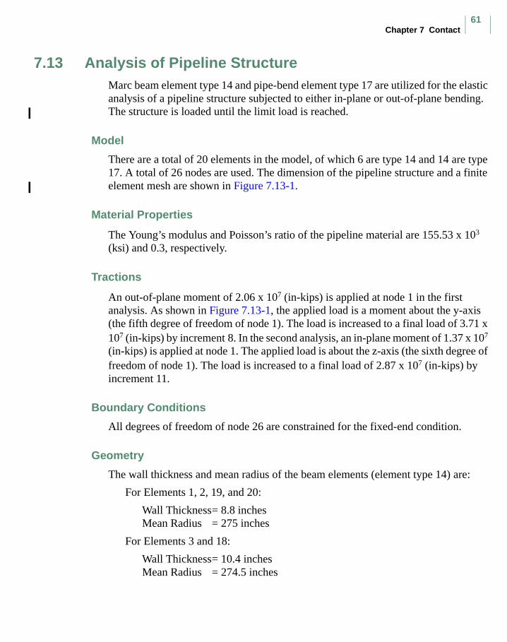
Chapter 7 Contact61
7.13 Analysis of Pipeline StructureMarc beam element type 14 and pipe-bend element type 17 are utilized for the elastic analysis of a pipeline structure subjected to either in-plane or out-of-plane bending. The structure is loaded until the limit load is reached.
Model
There are a total of 20 elements in the model, of which 6 are type 14 and 14 are type 17. A total of 26 nodes are used. The dimension of the pipeline structure and a finite element mesh are shown in Figure 7.13-1.
Material Properties
The Young’s modulus and Poisson’s ratio of the pipeline material are 155.53 x 10³ (ksi) and 0.3, respectively.
Tractions
An out-of-plane moment of 2.06 x 10⁷ (in-kips) is applied at node 1 in the first analysis. As shown in Figure 7.13-1, the applied load is a moment about the y-axis (the fifth degree of freedom of node 1). The load is increased to a final load of 3.71 x 10⁷ (in-kips) by increment 8. In the second analysis, an in-plane moment of 1.37 x 10⁷ (in-kips) is applied at node 1. The applied load is about the z-axis (the sixth degree of freedom of node 1). The load is increased to a final load of 2.87 x 10⁷ (in-kips) by increment 11.
Boundary Conditions
All degrees of freedom of node 26 are constrained for the fixed-end condition.
Geometry
The wall thickness and mean radius of the beam elements (element type 14) are:
For Elements 1, 2, 19, and 20:
Wall Thickness= 8.8 inchesMean Radius = 275 inches
For Elements 3 and 18:
Wall Thickness= 10.4 inchesMean Radius = 274.5 inches
MSC.Marc Volume E: Demostration Problems
62
For the pipe-bend elements (element type 17) the geometry data are:
Pipe thickness, t = 10.4 inchesThe angular extent of the pipe-bend section, φ = 90°The radius to the center of the pipe in the r-z plane, R= 838.2 inches
Results
In both analyses, the load is scaled such that incipient yield occurs at increment 1. The loading was increased until the limit load was reached. This was due to an inability to obtain a convergent solution. At the limit load, plasticity had occurred through all 11 layers through the thickness of the elbow section. Figure 7.13-2 shows the load-displacement results of this analysis. The special pipe bend element (type 17) allows the analyst to examine the ovalization of the cross section of the pipe. Using the SECTIONING option in the plot description section, we can examine this effect. Figure 7.13-3 shows the ovalization due to the two types of loading conditions.
Parameters, Options, and Subroutines Summary
Example e7x13b.dat:
Parameters Model Definition Options History Definition Options
ELEMENT CONNECTIVITY AUTO LOAD
ELSTO CONTROL CONTINUE
END COORDINATE PROPORTIONAL INCREMENT
SCALE END OPTION
SIZING FIXED DISP
TITLE GEOMETRY
ISOTROPIC
POINT LOAD
RESTART
TYING

Chapter 7 Contact63
Example e7x13c.dat:
Parameters Model Definition Options History Definition Options
ELEMENT CONNECTIVITY AUTO LOAD
ELSTO CONTROL CONTINUE
END COORDINATE PROPORTIONAL INCREMENT
SCALE END OPTION
SIZING FIXED DISP
TITLE GEOMETRY
ISOTROPIC
POINT LOAD
RESTART
TYING
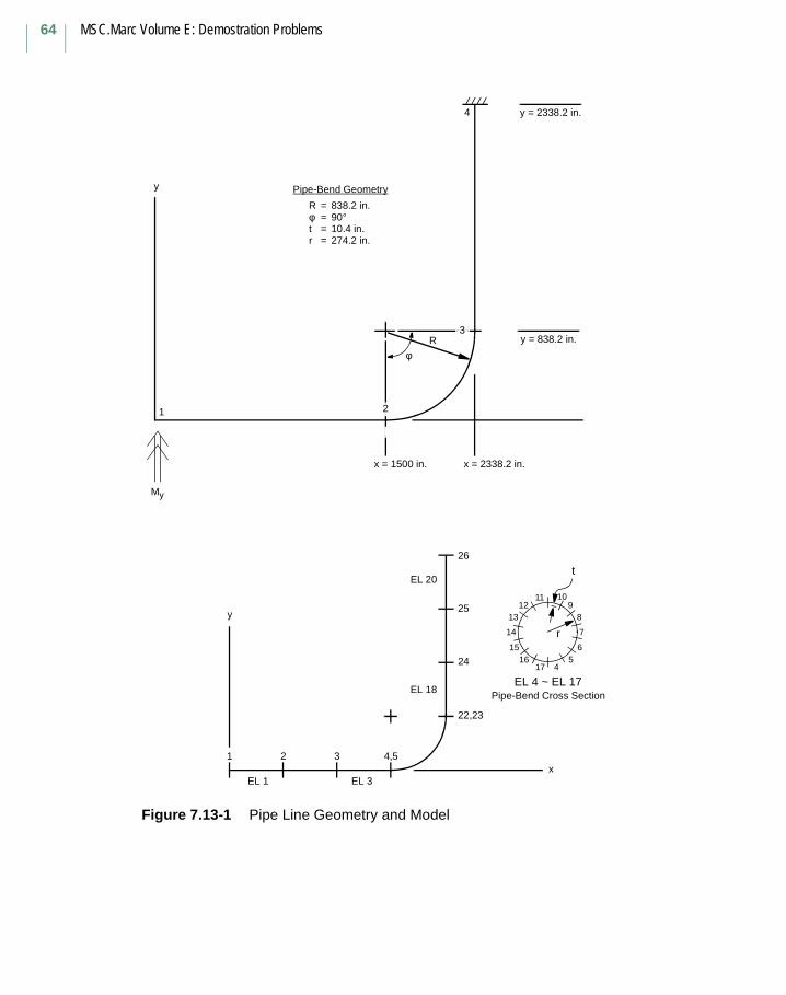
MSC.Marc Volume E: Demostration Problems
64
Figure 7.13-1 Pipe Line Geometry and Model
y = 2338.2 in.
y = 838.2 in.3
R
2
φ
x = 1500 in. x = 2338.2 in.
Pipe-Bend Geometry
R = 838.2 in.φ = 90°t = 10.4 in.r = 274.2 in.
4
y
26
25
24
22,23
EL 20
EL 18
y
1 2 3 4,5
EL 1 EL 3
1
My
109
8
7
65
4
1112
13
14
1516
17
t
r
EL 4 ~ EL 17Pipe-Bend Cross Section
x
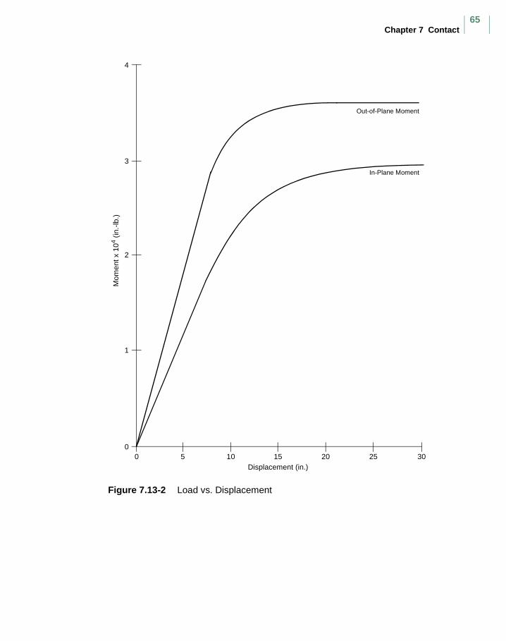
Chapter 7 Contact65
Figure 7.13-2 Load vs. Displacement
0250 5 10 15 20 30
Displacement (in.)
4
3
2
1
Mom
ent x
104 (
in.-
lb.)
Out-of-Plane Moment
In-Plane Moment
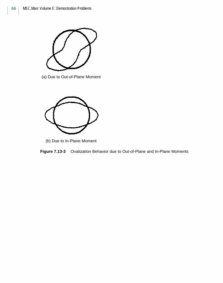
MSC.Marc Volume E: Demostration Problems
66
Figure 7.13-3 Ovalization Behavior due to Out-of-Plane and In-Plane Moments
(a) Due to Out-of-Plane Moment
(b) Due to In-Plane Moment
Chapter 7 Contact67
7.27 Twist and Extension of Circular Bar of Variable Thickness at Large Strains
This problem illustrates the use of Marc element 67, higher order axisymmetric with twist element, for a large strain elastic analysis of a circular bar of variable thickness. The bar is subjected to both a twist moment and an axial force at the free end of the circular bar. The tying constraint option is used to insure that the cross section at the small end of the bar remains flat. The material is modeled using Ogden model. The ELASTICITY,2 option is used to activate the updated Lagrangian formulation.
Element
Element type 67, an 8-node axisymmetric element with twist, is used in this example.
Model
There are 12 elements, with a total of 53 nodes. Dimensions of the circular bar and the finite element mesh are shown in Figure 7.27-1.
Material Properties
Ogden material properties are given as:
µ1 = 16 lb/in2, α1 = 2, µ2 = -4 lb/in2, α2 = -2.
Boundary Conditions
Degrees of freedom u and w are 0 at the fixed end (nodes 1-5). Symmetry conditions are imposed at r = 0 (v = 0).
Loading
In each increment, a 10 pound point load in the positive x-direction and a 4 inch per pound torque is applied at node 49. Due to the applied tying, the point load is distributed over the whole cross section.
Tying
Tying type 1 is used at the free end to simulate a generalized plane-strain condition in the z-direction. The tied nodes are 50, 51, 52, and 53 and the retained node is 49.
MSC.Marc Volume E: Demostration Problems
68
Results
The deformed mesh and the distribution of Equivalent von Mises stress is depicted in Figure 7.27-2.
Parameters, Options, and Subroutines Summary
Example e7x27.dat:
Parameters Model Definition Options History Definition Options
ALIAS CONNECTIVITY AUTO LOAD
ELASTICITY COORDINATE CONTINUE
ELEMENTS END OPTION CONTROL
END FIXED DISP POINT LOAD
LARGE DISP ISOTROPIC
SIZING OGDEN
TITLE POINT LOAD
POST
TYING
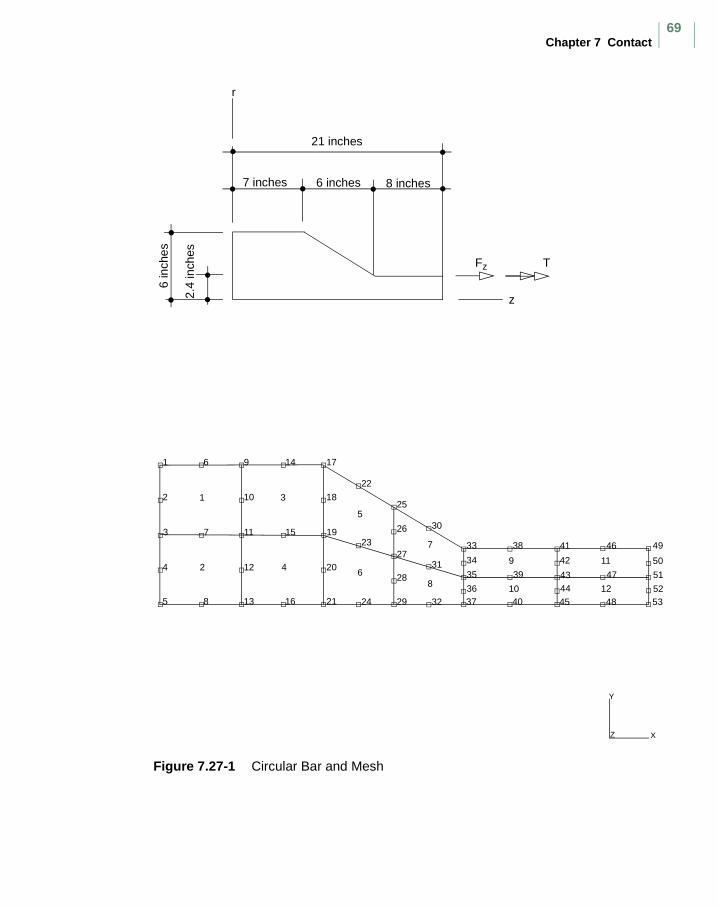
Chapter 7 Contact69
Figure 7.27-1 Circular Bar and Mesh
6 in
ches
2.4
inch
es7 inches 6 inches 8 inches
21 inches
Fz
z
T
r
1 6 9 14 17
3 7 11 15 19
4 2 12 4 20
5 8 13 16 21
1 3
24 29 37 40 45 48 53
35 39 43 47 51
34 9 42 11 50
33 38 41 46 497
22
255
2723
28
Y
XZ
2 10 18
6
26
8 3632
31
30
124410 52
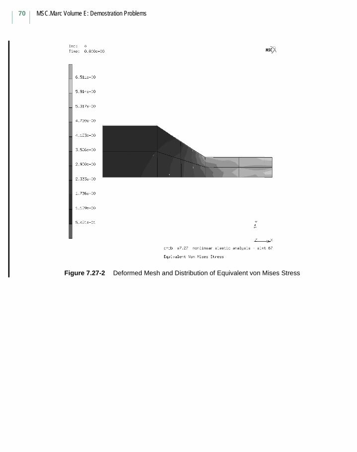
MSC.Marc Volume E: Demostration Problems
70
Figure 7.27-2 Deformed Mesh and Distribution of Equivalent von Mises Stress
Chapter 7 Contact71
7.28 Analysis of a Thick Rubber Cylinder Under Internal Pressure
In this example, the deformation of a thick rubber cylinder under internal pressure is modeled.
This problem illustrates the use of Marc elements types 10, 28, 55, and 116 (4- and 8-node axisymmetric elements with only displacement degrees of freedom at nodes) for rubber materials. Option ELASTICITY,2 is invoked to activate Marc updated Lagrangian formulation. The rubber material is modeled with either the Ogden or Mooney material models.
Element
Library element 10 is a 4-node bilinear axisymmetric element with displacements in radial and axial directions as degrees of freedom. Library element 116 is a 4-node bilinear, reduced integration, axisymmetric element with displacements in radial and axial directions as degrees of freedom. Library element 28 is a 8-node axisymmetric element with displacements in radial and axial directions as degrees of freedom. Library element 55 is a 8-node, reduced integration, axisymmetric element with displacements in radial and axial directions as degrees of freedom.
Model
The cylinder has an internal radius of 1 mm and an external radius of 2 mm. Figure 7.28-1 shows the initial mesh for the data sets using 8-noded elements.
Data SetElement Type(s)
Number of Elements
Number of Nodes
Differentiating Features
e7x28a 10 4 20 Odgen
e7x28b 116 4 10 Mooney
e7x28c 28 4 23 Ogden
e7x28d 55 4 23 Ogden
MSC.Marc Volume E: Demostration Problems
72
Material Properties
The Mooney material properties are given as:
C1 = 8 N/mm2, C2 = 2 N/mm2;
The Ogden material properties are given as:
µ1 = 16 N/mm2, α1 = 2, µ2 = 4 N/mm2, α2 = -2.
The bulk modulus is chosen as 200000 N/mm2, resulting in the ratio of K/G being 10000. The material is therefore highly incompressible. Both materials are equivalent.
Loads
A uniformly distributed internal pressure of 11.5 N/mm2 is applied on element number 1. This load is applied in increment zero. In Marc, increment zero is treated as linear. So an additional increment, with no additional load, is used to bring the solution to the correct nonlinear state.
Boundary Conditions
u = 0 on the planes z = 0 and z = 1.0 to simulate a plane strain condition.
Results
A. 8-Node Model (Element Type 28 and 55)
After the linear elastic step (increment 0), the radial displacements of the inside nodes for both elements 28 and 55 are 0.3833 mm.
They are the same as the analytical solution which predicts a radial displacement of 0.3833 mm.
After ten iterations, the radial displacement at the inside node is 1.0057 mm and the corresponding pressure can be computed from the following expression:
where A and B are the inner and outer radii of the cylinder in the undeformed state, “a” is the inner radius in the deformed state, and C1 and C2 are material constants.
The computed pressure of 11.5 N/mm2 is in very good agreement with the
prescribed value of 11.5 N/mm2.
P C1 C2+( ) logB
2a
2
A2
B2
A2
– a2
+( )-----------------------------------------
a
2A
2–( ) B
2A
2–( )
a2
B2
A2
– a2
+( )---------------------------------------------+=
Chapter 7 Contact73
B. 4-Node Model (Element Type 10 and 116)
After the linear elastic step (increment 0), the radial displacements of the inside nodes (nodes 1 and 6) are 0.3817 mm (for element type 10) and 0.3834 mm (for element type 116) respectively.
Agreement with analytical solution of 0.3833 mm is good. After ten iterations, the radial displacement at inside node is 1.0068 mm, and the
corresponding pressure is 11.5 N/mm2 for element 10. For element 116, the displacement at the inside node is 1.0063 mm and the corresponding pressure
is 11.5 N/mm2. Agreement with prescribed value of 11.5 N/mm2 is excellent.
Parameters, Options, and Subroutines Summary
Example e7x28a.dat:
Example e7x28b.dat:
Parameters Model Definition Options History Definition Options
ALIAS CONNECTIVITY CONTINUE
ELASTICITY CONTROL DIST LOAD
ELEMENTS COORDINATES
END DIST LOAD
FOLLOW FOR END OPTION
LARGE DISP FIXED DISP
SIZING OGDEN
TITLE POST
Parameters Model Definition Options History Definition Options
ALIAS CONNECTIVITY CONTINUE
ELASTICITY CONTROL DIST LOAD
ELEMENTS COORDINATES
END DIST LOAD
FOLLOW FOR END OPTION
LARGE DISP FIXED DISP
SIZING MOONEY
TITLE POST
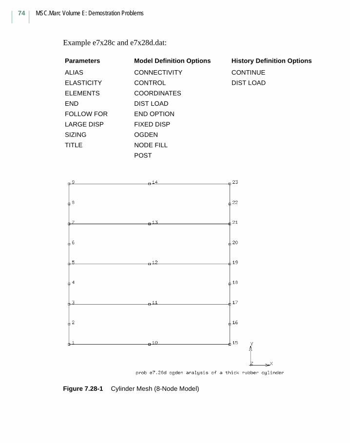
MSC.Marc Volume E: Demostration Problems
74
Example e7x28c and e7x28d.dat:
Figure 7.28-1 Cylinder Mesh (8-Node Model)
Parameters Model Definition Options History Definition Options
ALIAS CONNECTIVITY CONTINUE
ELASTICITY CONTROL DIST LOAD
ELEMENTS COORDINATES
END DIST LOAD
FOLLOW FOR END OPTION
LARGE DISP FIXED DISP
SIZING OGDEN
TITLE NODE FILL
POST
Chapter 7 Contact75
7.29 3-D Analyses of a Plate with a Hole at Large StrainsThis problem simulates the tensile loading of a plate with a hole at large strains. In e7x29a.dat, the HYPOELASTIC option and the user subroutine HYPELA2 are used to define constitutive behavior. Element type 7 is used and the material here is compressible. This job demonstrates the use of kinematics in defining user-defined material behavior. In e7x29b.dat, Element type 117 is used to model the plate (with the user-defined defaults file). The material in e7x29b.dat is modeled using Ogden model and is nearly incompressible.
In e7x29c.dat, element type 157 is used to model the plate. The material in e7x29c.dat is the same as for e7x29b.dat.
This problem is modeled using the two techniques summarized below.
Element
Library element 7 is a 8-node trilinear brick element with global displacements as degrees of freedom. Library element 117 is a 8-node trilinear brick element with reduced integration and global displacements as degrees of freedom. Library element type 157 is a 4+1-node, low-order tetrahedron using the Herrmann formulation.
Model
Due to symmetry of the geometry and loading, a quarter of the actual model is simulated. The finite element model is made up of 92 elements and 218 nodes. The finite element mesh is shown in Figure 7.29-1. The finite element mesh for e7x29c.dat is shown in Figure 7.29-2.
There are a total of 2902 nodes in the mesh. However, 2208 center nodes are condensed out on the element level and do not appear in the global matrix.
Geometry
The model is assumed to be a square of side 2 mm from which a quarter of a circle of radius 0.6 mm has been cut out. The initial thickness is 0.2 mm.
Data SetElement Type(s)
Number of Elements
Number of Nodes
Differentiating Features
e7x29a 7 92 218 HYPOELASTIC HYPELA2
e7x29b 117 92 218 user default file
e7x29c 157 2208 2902 element type 157

MSC.Marc Volume E: Demostration Problems
76
Material Properties
In e7x29a.dat, a quadratic-logarithmic, nonlinear elastic model with the initial bulk
modulus of 21666.67 N/mm2 and the initial shear modulus of 10000.00 N/mm2 is defined using the HYPOELASTIC option and the user subroutine HYPELA2. In
e7x29b.dat, the Ogden parameters are given as µ1=0.586 N/mm2, α1=2.0, µ2=-
0.354N/mm2, and α2=-2.0. The initial bulk modulus is 666666.667 N/mm2. The material properties for e7x29c.dat are the same as for e7x29b.dat.
Boundary Conditions and Loading
In addition to the boundary conditions due to symmetry, the third degree of freedom of the nodes located on the edges of the lower surface are fixed to avoid the rigid body motion in z-direction.
The loading is tensile. In e7x29a.dat, a uniform displacement of 1 mm is applied to one of the plate edges using 20 increments. The macroscopic total logarithmic strain is 40%. In e7x29b.dat, a uniform displacement of 2.5 mm is applied to one of the plate edges using 10 increments. The macroscopic total logarithmic strain is 81%.
In e7x29c.dat, the load in the form of the prescribed displacement is the same as for e7x29b.dat.
Results
The distribution of equivalent von Mises stress and the deformed model for e7x29a.dat after 20 increments is shown in Figure 7.29-3. The deformed model and the contour band plot of x displacements for e7x29b.dat and e7x29c.dat are shown in Figure 7.29-4 and Figure 7.29-5, respectively. Close agreement is observed.
Chapter 7 Contact77
Parameters, Options, and Subroutines Summary
Example e7x29a.dat:
User subroutine in u7x29a.f:HYPELA2
Example e7x29b.dat:
Parameters Model Definition Options History Definition Options
ELEMENTS CONNECTIVITY AUTO LOADEND CONTROL CONTINUELARGE DISP COORDINATES DISP CHANGEPROCESS END OPTIONSETNAME FIXED DISPSIZING GEOMETRYTITLE HYPOELASTICUPDATE OPTIMIZE
POST
Parameters Model Definition Options History Definition Options
ELEMENTS CONNECTIVITY AUTO LOADEND CONTROL CONTINUESETNAME COORDINATES DISP CHANGESIZING END OPTIONTITLE FIXED DISP
GEOMETRYOGDENOPTIMIZEPOST
MSC.Marc Volume E: Demostration Problems
78
User-defined Default Input e7x29_def.dat:
Example e7x29c.dat:
Parameters Model Definition Options
ALL POINTS END OPTION
ELASTICITY PARAMETER
END
LARGE DISP
PROCESS
Parameters Model Definition Options History Definition Options
ELEMENTS CONNECTIVITY AUTO LOAD
END CONTROL CONTINUE
LARGE DISP COORDINATES DISP CHANGE
SIZING END OPTION
TITLE FIXED DISP
NO PRINT
OGDEN
OPTIMIZE
POST
SOLVER
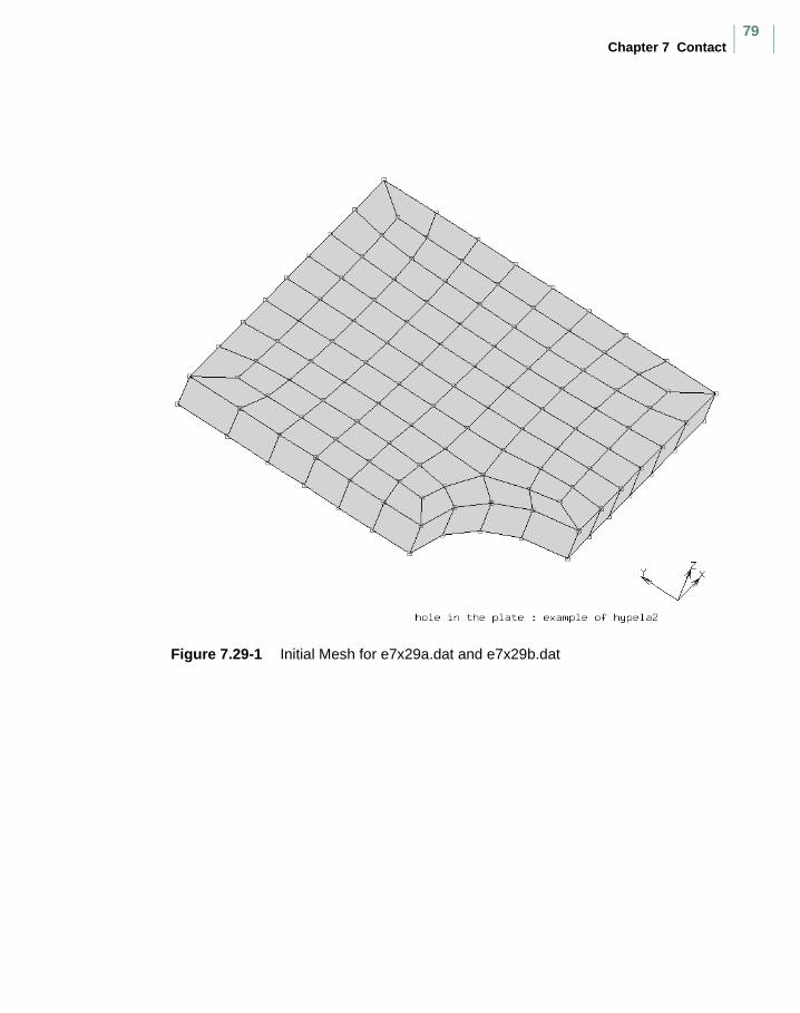
Chapter 7 Contact79
Figure 7.29-1 Initial Mesh for e7x29a.dat and e7x29b.dat
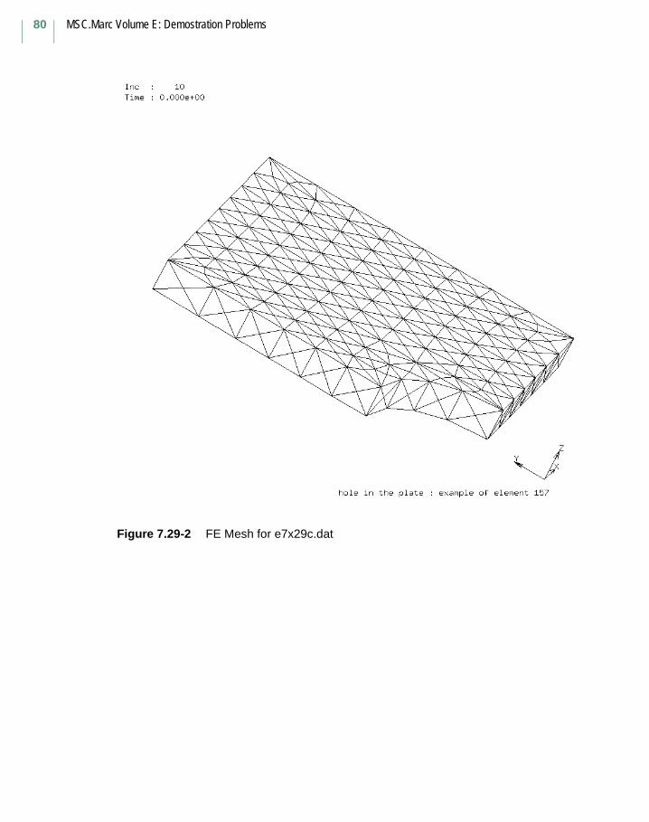
MSC.Marc Volume E: Demostration Problems
80
Figure 7.29-2 FE Mesh for e7x29c.dat
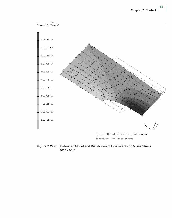
Chapter 7 Contact81
Figure 7.29-3 Deformed Model and Distribution of Equivalent von Mises Stress for e7x29a
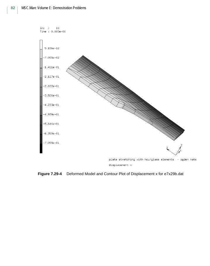
MSC.Marc Volume E: Demostration Problems
82
Figure 7.29-4 Deformed Model and Contour Plot of Displacement x for e7x29b.dat
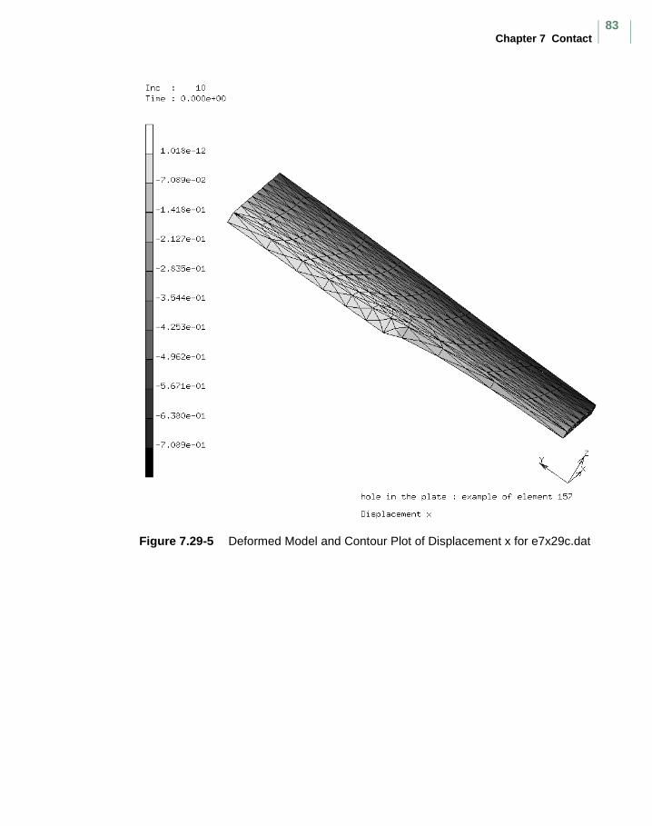
Chapter 7 Contact83
Figure 7.29-5 Deformed Model and Contour Plot of Displacement x for e7x29c.dat
MSC.Marc Volume E: Demostration Problems
84
7.32 Structural Relaxation of a Glass CubeFree structural relaxation of a glass cube subjected a cyclic temperature history, is simulated using Narayanaswamy model. This problem is modeled by means of element type 7.
The annealing of flat glass requires that the residual stresses be of an acceptable magnitude, while the specification for optical glass components usually includes a homogenous refractive index. The design of heat treated processes (for example, annealing) can be accomplished using the Narayanaswamy model. This allows you to study the time dependence of physical properties (for example, volumes) of glass subjected to a change in temperature.
The glass transition is a region of temperature in which molecular rearrangements occur on a scale of minutes or hours, so that the properties of a liquid change at a rate that is easily observed. Below the glass transition temperature, Tg, the material is extremely viscous and a solidus state exists. Above Tg the equilibrium structure is arrived at easily and the material is in liquidus state. Hence, the glass transition is revealed by a change in the temperature dependence of some property of a liquid during cooling. If a mechanical stress is applied to a liquid in the transition region, a time-dependent change in dimensions results due to the phenomenon of visco-elasticity.
If a liquid in the transition region is subjected to a sudden change in temperature, a time-dependent change in volume occurs. The latter process is called structural relaxation. Hence, structural relaxation governs the time-dependent response of a liquid to a change of temperature.
Element
Library element 7 is a 8-node trilinear brick element with global displacements as degrees of freedom.
Model
The side length of the glass cube is 2 mm. Because of the symmetry, only one eighth of the cube is modeled with one brick element.
Chapter 7 Contact85
Material Properties
The instantaneous moduli are given via ISOTROPIC option as: Young’s modulus is 5.58E4
N/mm2; Poisson’s ratio is 0.0814. The time dependent values are entered using VISCEPROP option as:
The solid and the liquid coefficients of the thermal expansion are chosen as 5.50E-7 and 1.93E-6, respectively. The weights and the reference relaxation times, used to define the response function, for each term in the series are input through SHIFT FUNCTION as:
Loads
An initial temperature of 6.20E2 is applied to the glass cube at increment 0. A cyclic temperature history is then applied: At first, the cube is gradually cooled down to 0.20E2 in 100 equal increments; Afterwards, it is heated up to the initial temperature at the equal incremental size.
Boundary Conditions
Boundary conditions are applied to the glass cube according to the symmetry.
Term No. Shear Constant Relaxation Time
1 1.08876E4 9.97000E-2
2 1.09134E4 9.40000E-3
3 3.97320E3 3.00000E-4
Term No. WeightReference
Relaxation Time
1 1.0800E-1 1.4780E+0
2 4.4300E-1 3.2970E-1
3 1.6600E-1 1.2130E-1
4 1.6100E-1 4.4600E-2
5 4.6000E-2 1,6400E-2
6 7.6000E-2 3.7000E-3
MSC.Marc Volume E: Demostration Problems
86
Results
Suppose a glass is equilibrated at temperature T1, and suddenly cooled to T2 at t0. The instantaneous change in volume is αg(T2 - T1), followed by relaxation towards the equilibrium value V(∞,T2). The total change in volume due to the temperature change is αl(T2 - T1) as shown in Figure 7.32-1b. The rate of volume change depends on a characteristic time called the relaxation time.
The slope of dV/dT changes from the high value characteristic of the fluid αl to the low characteristic of the glass αg as shown in Figure 7.32-2. The glass transition temperature Tg is a point in the center of the transition region. The low-temperature slope αg represents the change in volume V caused by vibration of the atoms in their potential wells. In the (glassy) temperature range, the atoms are frozen into a particular configuration. As the temperature T increases, the atoms acquire enough energy to break bonds and rearrange into new structures. That allows the volume to increase more rapidly, so αl > αg. The difference α = αl - αg represents the structural contribution to the volume.
When a liquid is cooled and reheated, a hysteresis is observed.
The volume change of the glass cube with the change of the temperature 1 as calculated by Marc, is illustrated in Figure 7.32-3. The hysteresis shown in Figure 7.32-3 indicates the calculations are in a good qualitative agreement with experimental observations.
Parameters, Options, and Subroutines Summary
Example e7x32.dat:
Parameters Model Definition Options History Definition Options
ALL POINTS CHANGE STATE AUTO LOADELEMENTS CONNECTIVITY CHANGE STATEEND COORDINATES CONTINUESETNAME END OPTIONS CONTROLSIZING FIXED DISP TIME STEPSTATE VARS ISOTROPICTITLE OPTIMIZE
PRINT CHOICEPOSTSHIFT FUNCTIONSOLVERVISCEL EXPVISCELPROP$NO PRINT
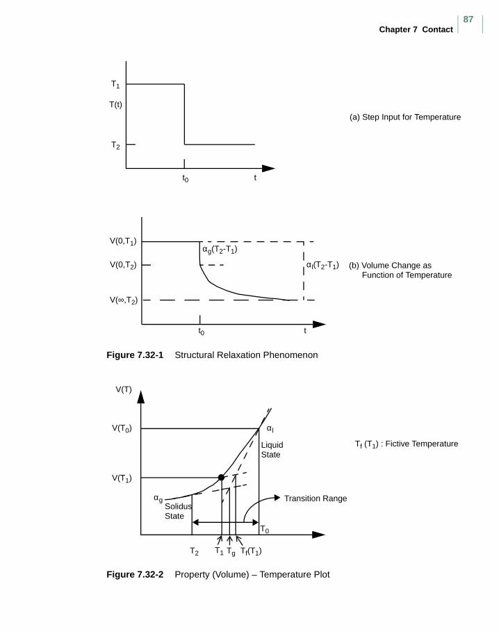
Chapter 7 Contact87
Figure 7.32-1 Structural Relaxation Phenomenon
Figure 7.32-2 Property (Volume) – Temperature Plot
T1
T2
t0
T(t)
V(0,T1)
V(∞,T2)
V(0,T2)
t0 t
t
αg(T2-T1)
αl(T2-T1)
(a) Step Input for Temperature
(b) Volume Change as Function of Temperature
V(T)
V(T1)
T2 Tg Tf(T1)
αg
αl
SolidusState
LiquidState
Transition Range
Tf (T1) : Fictive Temperature
V(T0)
T0
T1
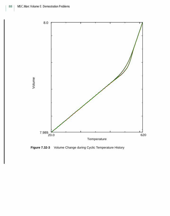
MSC.Marc Volume E: Demostration Problems
88
Figure 7.32-3 Volume Change during Cyclic Temperature History
20.0 620Temperature
7.989
8.0
Vol
ume

Chapter 8 Advanced Topics89
Chapter 8 Advanced Topics

MSC.Marc Volume E: Demostration Problems
90
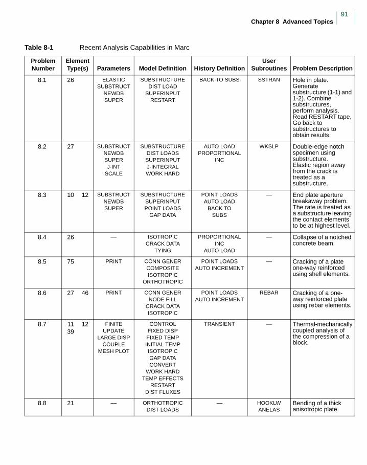
Chapter 8 Advanced Topics91
Table 8-1 Recent Analysis Capabilities in Marc
Problem Number
Element Type(s) Parameters Model Definition History Definition
User Subroutines Problem Description
8.1 26 ELASTICSUBSTRUCT
NEWDBSUPER
SUBSTRUCTUREDIST LOAD
SUPERINPUTRESTART
BACK TO SUBS SSTRAN Hole in plate. Generate substructure (1-1) and 1-2). Combine substructures, perform analysis.Read RESTART tape, Go back to substructures to obtain results.
8.2 27 SUBSTRUCTNEWDBSUPERJ-INT
SCALE
SUBSTRUCTUREDIST LOADSSUPERINPUTJ-INTEGRALWORK HARD
AUTO LOADPROPORTIONAL
INC
WKSLP Double-edge notch specimen using substructure.Elastic region away from the crack is treated as a substructure.
8.3 10 12 SUBSTRUCTNEWDBSUPER
SUBSTRUCTURESUPERINPUTPOINT LOADS
GAP DATA
POINT LOADSAUTO LOAD
BACK TOSUBS
–– End plate aperture breakaway problem.The rate is treated as a substructure leaving the contact elements to be at highest level.
8.4 26 –– ISOTROPICCRACK DATA
TYING
PROPORTIONAL INC
AUTO LOAD
–– Collapse of a notched concrete beam.
8.5 75 PRINT CONN GENERCOMPOSITEISOTROPIC
ORTHOTROPIC
POINT LOADSAUTO INCREMENT
–– Cracking of a plate one-way reinforced using shell elements.
8.6 27 46 PRINT CONN GENERNODE FILL
CRACK DATAISOTROPIC
POINT LOADSAUTO INCREMENT
REBAR Cracking of a one-way reinforced plate using rebar elements.
8.7 11 1239
FINITEUPDATE
LARGE DISPCOUPLE
MESH PLOT
CONTROLFIXED DISPFIXED TEMPINITIAL TEMPISOTROPICGAP DATACONVERT
WORK HARDTEMP EFFECTS
RESTARTDIST FLUXES
TRANSIENT –– Thermal-mechanically coupled analysis of the compression of a block.
8.8 21 –– ORTHOTROPICDIST LOADS
–– HOOKLWANELAS
Bending of a thick anisotropic plate.
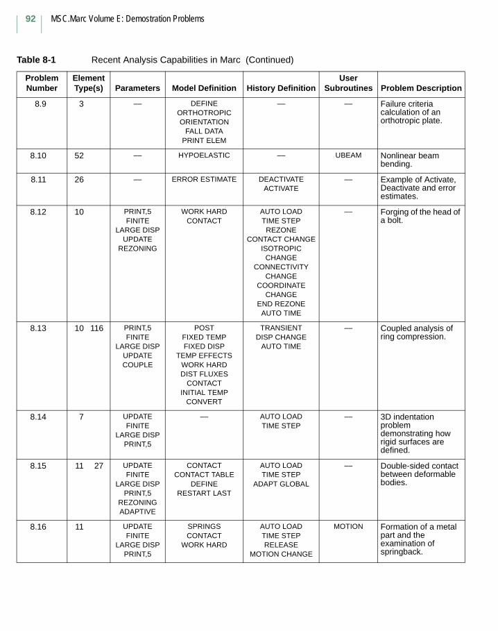
MSC.Marc Volume E: Demostration Problems
92
8.9 3 –– DEFINEORTHOTROPICORIENTATION
FALL DATAPRINT ELEM
–– –– Failure criteria calculation of an orthotropic plate.
8.10 52 –– HYPOELASTIC –– UBEAM Nonlinear beam bending.
8.11 26 –– ERROR ESTIMATE DEACTIVATEACTIVATE
–– Example of Activate, Deactivate and error estimates.
8.12 10 PRINT,5FINITE
LARGE DISPUPDATE
REZONING
WORK HARDCONTACT
AUTO LOADTIME STEP
REZONECONTACT CHANGE
ISOTROPIC CHANGE
CONNECTIVITY CHANGE
COORDINATE CHANGE
END REZONEAUTO TIME
–– Forging of the head of a bolt.
8.13 10 116 PRINT,5FINITE
LARGE DISPUPDATECOUPLE
POSTFIXED TEMPFIXED DISP
TEMP EFFECTSWORK HARDDIST FLUXES
CONTACTINITIAL TEMP
CONVERT
TRANSIENTDISP CHANGE
AUTO TIME
–– Coupled analysis of ring compression.
8.14 7 UPDATEFINITE
LARGE DISPPRINT,5
–– AUTO LOADTIME STEP
–– 3D indentation problem demonstrating how rigid surfaces are defined.
8.15 11 27 UPDATEFINITE
LARGE DISPPRINT,5
REZONINGADAPTIVE
CONTACTCONTACT TABLE
DEFINERESTART LAST
AUTO LOADTIME STEP
ADAPT GLOBAL
–– Double-sided contact between deformable bodies.
8.16 11 UPDATEFINITE
LARGE DISPPRINT,5
SPRINGSCONTACT
WORK HARD
AUTO LOADTIME STEPRELEASE
MOTION CHANGE
MOTION Formation of a metal part and the examination of springback.
Table 8-1 Recent Analysis Capabilities in Marc (Continued)
Problem Number
Element Type(s) Parameters Model Definition History Definition
User Subroutines Problem Description
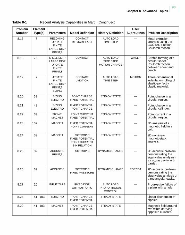
Chapter 8 Advanced Topics93
8.17 7 REZONINGUPDATEFINITE
LARGE DISPPRINT,8
CONTACTRESTART LAST
AUTO LOADTIME STEP
–– Metal extrusion analysis using the CONTACT option. Coulomb friction.
8.18 75 SHELL SET,7LARGE DISP
UPDATEFINITE
PRINT,8
CONTACT AUTO LOADTIME STEP
MOTION CHANGE
WKSLP Stretch forming of a circular sheet. Coulomb friction between sheet and punch.
8.19 7 UPDATEFINITE
LARGE DISPPRINT,8SIZING
CONTACTUMOTION
AUTO LOADTIME STEP
MOTION Three dimensional indentation rolling of elastic-perfectly plastic material.
8.20 39 SIZINGELECTRO
POINT CHARGEFIXED POTENTIAL
STEADY STATE –– Point charge in a circular region.
8.21 43 SIZINGELECTRO
FIXED POTENTIALPOINT CHARGE
STEADY STATE –– Point charge in a circular cylinder.
8.22 39 SIZING\MAGNET
POINT CURRENTFIXED POTENTIAL
STEADY STATE –– Point current in a circular region.
8.23 109 MAGNET FIXED POTENTIALPOINT CURRENT
STEADY STATE –– 3D analysis of a magnetic field in a coil.
8.24 39 MAGNET ISOTROPICFIXED POTENTIALPOINT CURRENT
B-H RELATION
STEADY STATE –– 2D nonlinear magnetostatic analysis.
8.25 39 ACOUSTICPRINT,3
ISOTROPIC DYNAMIC CHANGE –– 2D acoustic problem demonstrating the eigenvalue analysis in a circular cavity with barrier.
8.26 39 ACOUSTIC ISOTROPICFIXED PRESSURE
DYNAMIC CHANGE FORCDT 2D acoustic problem demonstrating the eigenvalue analysis of a rectangular cavity.
8.27 26 INPUT TAPE FIXED DISPORTHOTROPIC
AUTO LOADPROPORTIONAL
CONTROL
–– Progressive failure of a plate with a hole.
8.28 41 103 ELECTRO POINT CHARGEFIXED POTENTIAL
STEADY STATE –– Linear distribution of dipoles.
8.29 41 103 MAGNET POINT CHARGEFIXED POTENTIAL
STEADY STATE –– Magnetic field around two wires carrying opposite currents.
Table 8-1 Recent Analysis Capabilities in Marc (Continued)
Problem Number
Element Type(s) Parameters Model Definition History Definition
User Subroutines Problem Description
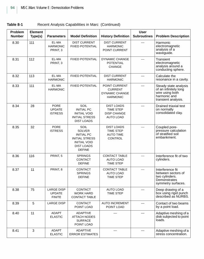
MSC.Marc Volume E: Demostration Problems
94
8.30 111 EL-MAHARMONIC
PRINT, 3
DIST CURRENTFIXED POTENTIAL
DIST CURRENTHARMONIC
POINT CURRENT
–– Harmonic electromagnetic analysis of a waveguide.
8.31 112 EL-MAPRINT, 3
FIXED POTENTIAL DYNAMIC CHANGEPOTENTIAL
CHANGE
–– Transient electromagnetic analysis around a conducting sphere.
8.32 113 EL-MAHARMONIC
FIXED POTENTIAL DIST CURRENT HARMONIC
–– Calculate the resonance in a cavity.
8.33 111 EL-MAHARMONIC
FIXED POTENTIAL POINT CURRENTCURRENT
DYNAMIC CHANGEHARMONIC
–– Steady state analysis of an infinitely long wire using both harmonic and transient analysis.
8.34 28 POREUPDATEISTRESS
SOILINITIAL PC
INITIAL VOIDINITIAL STRESS
DIST LOADS
DIST LOADSTIME STEP
DISP CHANGEAUTO LOAD
–– Drained triaxial test on normally consolidated clay.
8.35 32 POREISTRESS
SOILSOLVER
INITIAL PCINITIAL STRESS
INITIAL VOIDDIST LOADS
DEFINE
DIST LOADSTIME STEPAUTO TIMECONTROL
–– Coupled pore-pressure calculation of stratified soil embankment.
8.36 116 PRINT, 5 SPRINGSCONTACTDEFINE
CONTACT TABLEAUTO LOADTIME STEP
–– Interference fit of two cylinders.
8.37 11 PRINT, 8 CONTACTSPRINGSDEFINE
CONTACT TABLEAUTO LOADTIME STEP
–– Interference fit between sectors of two cylinders. Demonstrates symmetry surfaces.
8.38 75 LARGE DISPUPDATEFINITE
CONTACTWORK HARD
CONTACT TABLE
AUTO LOADTIME STEP
–– Deep drawing of a box using rigid punch described as NURBS.
8.39 5 LARGE DISP CONTACTPOINT LOAD
AUTO INCREMENTPOINT LOAD
–– Contact of two beams by a point load.
8.40 11 ADAPTELASTIC
ADAPTIVEATTACH NODES
SURFACEPOINT LOAD
–– –– Adaptive meshing of a disk subjected to point loads.
8.41 3 ADAPTELASTIC
ADAPTIVEERROR ESTIMATES
–– –– Adaptive meshing of a stress concentration.
Table 8-1 Recent Analysis Capabilities in Marc (Continued)
Problem Number
Element Type(s) Parameters Model Definition History Definition
User Subroutines Problem Description
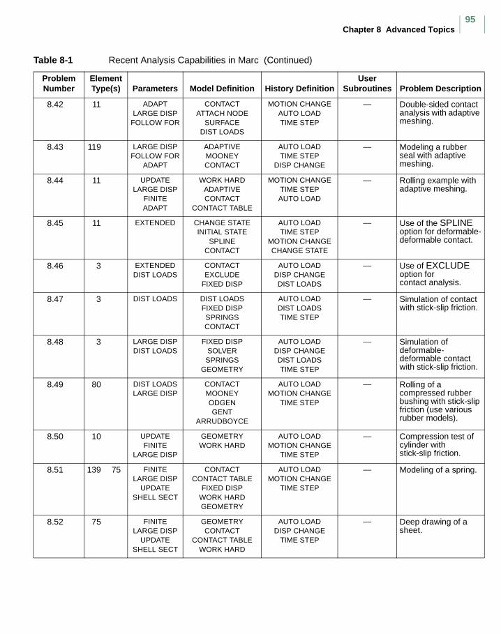
Chapter 8 Advanced Topics95
8.42 11 ADAPTLARGE DISP
FOLLOW FOR
CONTACTATTACH NODE
SURFACEDIST LOADS
MOTION CHANGEAUTO LOADTIME STEP
–– Double-sided contact analysis with adaptive meshing.
8.43 119 LARGE DISPFOLLOW FOR
ADAPT
ADAPTIVEMOONEYCONTACT
AUTO LOADTIME STEP
DISP CHANGE
–– Modeling a rubber seal with adaptive meshing.
8.44 11 UPDATELARGE DISP
FINITEADAPT
WORK HARDADAPTIVECONTACT
CONTACT TABLE
MOTION CHANGETIME STEPAUTO LOAD
–– Rolling example with adaptive meshing.
8.45 11 EXTENDED CHANGE STATEINITIAL STATE
SPLINECONTACT
AUTO LOADTIME STEP
MOTION CHANGECHANGE STATE
–– Use of the SPLINE option for deformable-deformable contact.
8.46 3 EXTENDEDDIST LOADS
CONTACTEXCLUDE
FIXED DISP
AUTO LOADDISP CHANGEDIST LOADS
–– Use of EXCLUDE option for contact analysis.
8.47 3 DIST LOADS DIST LOADSFIXED DISPSPRINGSCONTACT
AUTO LOADDIST LOADSTIME STEP
–– Simulation of contact with stick-slip friction.
8.48 3 LARGE DISPDIST LOADS
FIXED DISPSOLVERSPRINGS
GEOMETRY
AUTO LOADDISP CHANGEDIST LOADSTIME STEP
–– Simulation of deformable-deformable contact with stick-slip friction.
8.49 80 DIST LOADSLARGE DISP
CONTACTMOONEYODGENGENT
ARRUDBOYCE
AUTO LOADMOTION CHANGE
TIME STEP
–– Rolling of a compressed rubber bushing with stick-slip friction (use various rubber models).
8.50 10 UPDATEFINITE
LARGE DISP
GEOMETRYWORK HARD
AUTO LOADMOTION CHANGE
TIME STEP
–– Compression test of cylinder with stick-slip friction.
8.51 139 75 FINITELARGE DISP
UPDATESHELL SECT
CONTACTCONTACT TABLE
FIXED DISPWORK HARDGEOMETRY
AUTO LOADMOTION CHANGE
TIME STEP
–– Modeling of a spring.
8.52 75 FINITELARGE DISP
UPDATESHELL SECT
GEOMETRYCONTACT
CONTACT TABLEWORK HARD
AUTO LOADDISP CHANGE
TIME STEP
–– Deep drawing of a sheet.
Table 8-1 Recent Analysis Capabilities in Marc (Continued)
Problem Number
Element Type(s) Parameters Model Definition History Definition
User Subroutines Problem Description
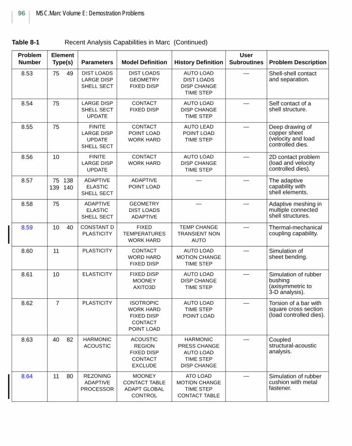
MSC.Marc Volume E: Demostration Problems
96
8.53 75 49 DIST LOADSLARGE DISPSHELL SECT
DIST LOADSGEOMETRYFIXED DISP
AUTO LOADDIST LOADS
DISP CHANGETIME STEP
–– Shell-shell contact and separation.
8.54 75 LARGE DISPSHELL SECT
UPDATE
CONTACTFIXED DISP
AUTO LOADDISP CHANGE
TIME STEP
–– Self contact of a shell structure.
8.55 75 FINITELARGE DISP
UPDATESHELL SECT
CONTACTPOINT LOADWORK HARD
AUTO LEADPOINT LOADTIME STEP
–– Deep drawing of copper sheet (velocity and load controlled dies.
8.56 10 FINITELARGE DISP
UPDATE
CONTACTWORK HARD
AUTO LOADDISP CHANGE
TIME STEP
–– 2D contact problem (load and velocity controlled dies).
8.57 75 138139 140
ADAPTIVEELASTIC
SHELL SECT
ADAPTIVEPOINT LOAD
–– –– The adaptive capability with shell elements.
8.58 75 ADAPTIVEELASTIC
SHELL SECT
GEOMETRYDIST LOADSADAPTIVE
–– –– Adaptive meshing in multiple connected shell structures.
8.59 10 40 CONSTANT DPLASTICITY
FIXED TEMPERATURES
WORK HARD
TEMP CHANGETRANSIENT NON
AUTO
–– Thermal-mechanical coupling capability.
8.60 11 PLASTICITY CONTACTWORD HARDFIXED DISP
AUTO LOADMOTION CHANGE
TIME STEP
–– Simulation of sheet bending.
8.61 10 ELASTICITY FIXED DISPMOONEYAXITO3D
AUTO LOADDISP CHANGE
TIME STEP
–– Simulation of rubber bushing (axisymmetric to 3-D analysis).
8.62 7 PLASTICITY ISOTROPICWORK HARDFIXED DISPCONTACT
POINT LOAD
AUTO LOADTIME STEP
POINT LOAD
–– Torsion of a bar with square cross section (load controlled dies).
8.63 40 82 HARMONICACOUSTIC
ACOUSTICREGION
FIXED DISPCONTACTEXCLUDE
HARMONICPRESS CHANGE
AUTO LOADTIME STEP
DISP CHANGE
–– Coupled structural-acoustic analysis.
8.64 11 80 REZONINGADAPTIVE
PROCESSOR
MOONEYCONTACT TABLEADAPT GLOBAL
CONTROL
ATO LOADMOTION CHANGE
TIME STEPCONTACT TABLE
–– Simulation of rubber cushion with metal fastener.
Table 8-1 Recent Analysis Capabilities in Marc (Continued)
Problem Number
Element Type(s) Parameters Model Definition History Definition
User Subroutines Problem Description
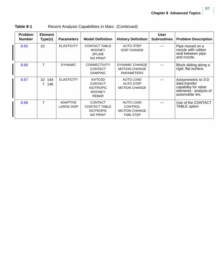
Chapter 8 Advanced Topics97
8.65 10 ELASTICITY CONTACT TABLEMOONEYSPLINE
NO PRINT
AUTO STEPDISP CHANGE
–– Pipe moved on a nozzle with rubber seal between pipe and nozzle.
8.66 7 DYNAMIC CONNECTIVITYCONTACTDAMPING
DYNAMIC CHANGEMOTION CHANGE
PARAMETERS
–– Block sliding along a rigid, flat surface.
8.67 10 1447 146
ELASTICITY AXITO3DCONTACT
ISOTROPICMOONEYREBAR
AUTO LOADAUTO STEP
MOTION CHANGE
–– Axisymmetric to 3-D data transfer capability for rebar elements - analysis of automobile tire.
8.68 7 ADAPTIVELARGE DISP
CONTACTCONTACT TABLE
ISOTROPICNO PRINT
AUTO LOADCONTROL
MOTION CHANGETIME STEP
–– Use of the CONTACT TABLE option
Table 8-1 Recent Analysis Capabilities in Marc (Continued)
Problem Number
Element Type(s) Parameters Model Definition History Definition
User Subroutines Problem Description
MSC.Marc Volume E: Demostration Problems
98
8.33 Coupled Analysis of Ring CompressionThis example demonstrates Marc’s ability to perform a large deformation problem, incorporating thermal mechanical coupling and automated contact.
A ring of aluminum is deformed by a block of steel. Both have the capacity to deform, and possibly, slide between each other.
Coupling
There are several sources of coupling in this analysis.
1. As the temperature changes, thermal stresses are developed due to nonzero coefficient of thermal expansion.
2. As the temperature changes, the mechanical properties change. It happens in this case because of the temperature-dependent flow stress.
3. As the geometry changes, the heat transfer problem changes. This includes changes in the contacting interface.
4. As plastic work is performed, internal heat is generated.
5. As the bodies slide, friction generates heat.
Parameters
The UPDATE, FINITE, and LARGE DISP parameters indicate this is a finite deformation analysis.The COUPLE option is used to indicate that a coupled thermal-mechanical analysis is being performed. A four-node bilinear axisymmetric element is used. The PRINT,5 option requests additional information in the output regarding nodes acquiring or losing contact.
Mesh Definition
Mentat was used to create the mesh. There are separate nodes along both sides of the contact interface so that sliding is possible. Due to symmetry, only one quarter of the region is modeled. The mesh is shown (with the units in mm) in Figure 8.13-1. In a coupled analysis, a displacement element automatically produces the coupled (displacement-temperature) formulation to be used.
This analysis is performed using both element type 10 and element type 116. Both elements are four-node axisymmetric elements. Element type 116 uses a single integration point and an hourglass stiffness stabilization procedure.
Chapter 8 Advanced Topics99
The standard CONTACT option is used. Free surfaces can have convection heat transfer to the environment. As soon as contact is detected, a contact thermal barrier, defined by means of a film coefficient, starts operating.
Geometry
A ‘1’ is placed in the second field to indicate that the constant dilatation formulation is used. This is not necessary for the analysis using element type 116.
Boundary Conditions
Symmetry displacement boundary conditions are imposed on the ring meridian plane and on the block axis. The block is moved down by application of displacement boundary conditions to the face opposite to the contact face. The displacement boundary conditions are entered in the FIXED DISPLACEMENT option. On the outside surface of the block, the temperature is constrained to 20°C, to simulate a much larger size block. This is done with the FIXED TEMPERATURE option.
Control Options
A formatted post file containing stress components and effective plastic strain is written at the end of 50 increments. The NO PRINT option limits the amount of output to a minimum. Displacement control is used in the deformation part of the analysis with a relative error of 15%. As far as the heat transfer part of the analysis is concerned, a 10°C maximum error in temperature estimate is entered. Even if thermal material properties are not temperature-dependent, this provides a means of forcing recycling when heat transfer between two bodies produces large variations of temperature per increment.
Initial Conditions
The ring is given an initial temperature of 427°C, and the block is given an initial temperature of 20°C.
Material Properties
The ring is treated as an elastic-plastic material with a Young’s modulus of 10,000 MPa, a Poisson’s ratio of 0.33, a coefficient of thermal expansion of 1.3 x 10⁻⁵ mm/mm°C, and an initial yield stress of 3.4 MPa, corresponding to a reference temperature of 200°C. The material workhardens from the initial yield stress to a yield stress of 5.78 MPa for strains above 70%, according to a piecewise linear function entered via
MSC.Marc Volume E: Demostration Problems
100
WORK HARD DATA. The flow stress and work hardening slope decrease with temperature increases at a rate of 0.007 MPa per degree. The thermal properties are conductivity of 242.0 N/s°C and specific heat of 2.4255 Nmm/g°C.
The block is treated as an elastic material with a Young’s modulus of 100,000 MPa, a Poisson’s ratio of 0.333. The thermal properties are conductivity of 19.0 N/s°C and specific heat of 3.77 Nmm/g°C.
Distributed Flux
This distributed flux block is used to indicate that internal heat is generated due to plastic deformation.
Convert
The option is used to give the conversion factor between the mechanical energy and the thermal energy.
The internal volumetric flux per unit volume becomes:
φ = cwp
where wp is the plastic strain energy density.
Contact
The CONTACT option declares that there are two bodies with adhesive friction between them. Marc calculates the contact tolerance.
The first body is deformable and is made of the elements of the ring. There is no need to specify any motion. The ring’s free surfaces have convection heat transfer defined by a film coefficient of 0.01, and a sink temperature of 20°C. The second body is also deformable and made out of the elements of the block. A reference point and an axial velocity are given, although they are not used in the calculations; this is done as a reminder of what the imposed boundary conditions are simulating. A friction coefficient of 0.5 defines the interface friction conditions, based on the cohesive model. The block’s free surfaces have convection heat transfer defined by a film coefficient of 0.01 N/s-mm°C, and a sink temperature of 20°C. The contact surfaces have a thermal barrier defined by a film coefficient of 35.
This ordering of the two bodies results in imposing the constraint so that the nodes of the ring do not penetrate the surface of the block. Friction and thermal barrier at the interface use data taken from the body defining the block.
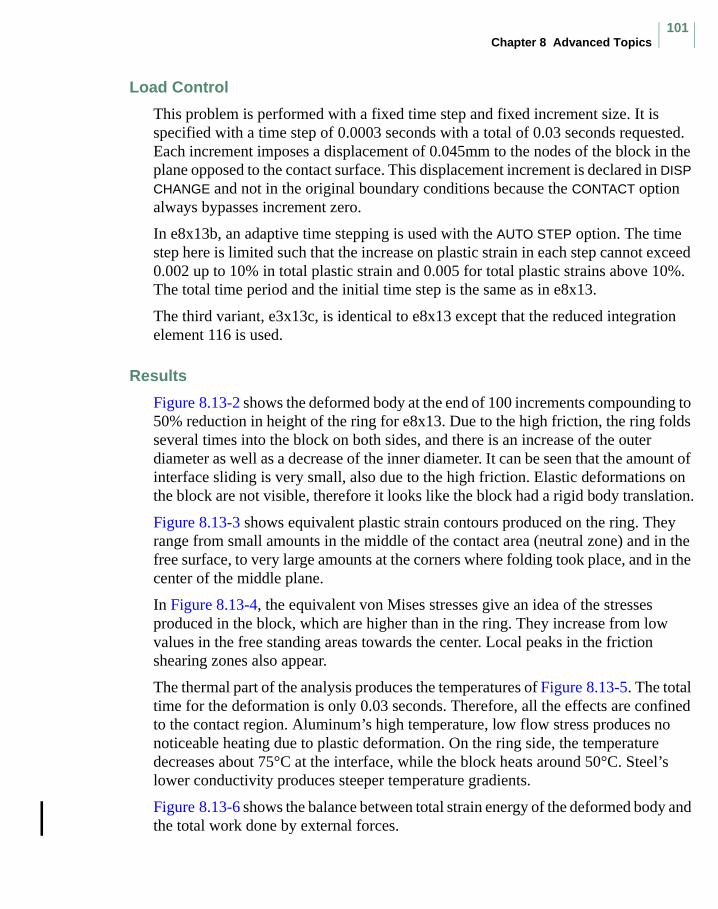
Chapter 8 Advanced Topics101
Load Control
This problem is performed with a fixed time step and fixed increment size. It is specified with a time step of 0.0003 seconds with a total of 0.03 seconds requested. Each increment imposes a displacement of 0.045mm to the nodes of the block in the plane opposed to the contact surface. This displacement increment is declared in DISP CHANGE and not in the original boundary conditions because the CONTACT option always bypasses increment zero.
In e8x13b, an adaptive time stepping is used with the AUTO STEP option. The time step here is limited such that the increase on plastic strain in each step cannot exceed 0.002 up to 10% in total plastic strain and 0.005 for total plastic strains above 10%. The total time period and the initial time step is the same as in e8x13.
The third variant, e3x13c, is identical to e8x13 except that the reduced integration element 116 is used.
Results
Figure 8.13-2 shows the deformed body at the end of 100 increments compounding to 50% reduction in height of the ring for e8x13. Due to the high friction, the ring folds several times into the block on both sides, and there is an increase of the outer diameter as well as a decrease of the inner diameter. It can be seen that the amount of interface sliding is very small, also due to the high friction. Elastic deformations on the block are not visible, therefore it looks like the block had a rigid body translation.
Figure 8.13-3 shows equivalent plastic strain contours produced on the ring. They range from small amounts in the middle of the contact area (neutral zone) and in the free surface, to very large amounts at the corners where folding took place, and in the center of the middle plane.
In Figure 8.13-4, the equivalent von Mises stresses give an idea of the stresses produced in the block, which are higher than in the ring. They increase from low values in the free standing areas towards the center. Local peaks in the friction shearing zones also appear.
The thermal part of the analysis produces the temperatures of Figure 8.13-5. The total time for the deformation is only 0.03 seconds. Therefore, all the effects are confined to the contact region. Aluminum’s high temperature, low flow stress produces no noticeable heating due to plastic deformation. On the ring side, the temperature decreases about 75°C at the interface, while the block heats around 50°C. Steel’s lower conductivity produces steeper temperature gradients.
Figure 8.13-6 shows the balance between total strain energy of the deformed body and the total work done by external forces.
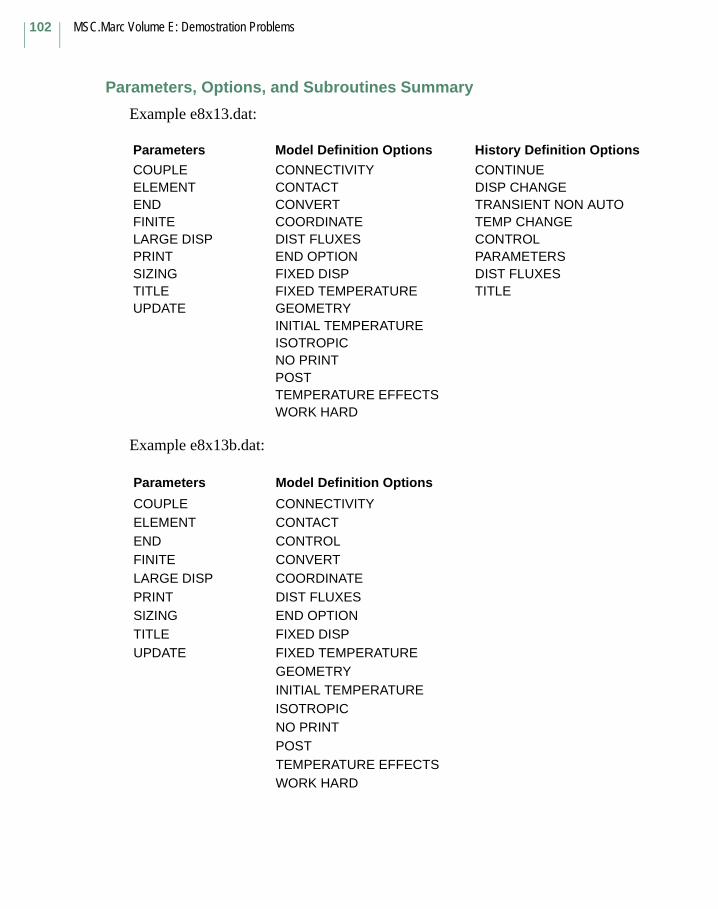
MSC.Marc Volume E: Demostration Problems
102
Parameters, Options, and Subroutines Summary
Example e8x13.dat:
Example e8x13b.dat:
Parameters Model Definition Options History Definition Options
COUPLE CONNECTIVITY CONTINUEELEMENT CONTACT DISP CHANGEEND CONVERT TRANSIENT NON AUTOFINITE COORDINATE TEMP CHANGELARGE DISP DIST FLUXES CONTROLPRINT END OPTION PARAMETERSSIZING FIXED DISP DIST FLUXESTITLE FIXED TEMPERATURE TITLEUPDATE GEOMETRY
INITIAL TEMPERATUREISOTROPICNO PRINTPOSTTEMPERATURE EFFECTSWORK HARD
Parameters Model Definition Options
COUPLE CONNECTIVITYELEMENT CONTACTEND CONTROLFINITE CONVERTLARGE DISP COORDINATEPRINT DIST FLUXESSIZING END OPTIONTITLE FIXED DISPUPDATE FIXED TEMPERATURE
GEOMETRY INITIAL TEMPERATURE ISOTROPIC NO PRINT POST TEMPERATURE EFFECTS WORK HARD

Chapter 8 Advanced Topics103
Example e8x13c.dat:
Figure 8.13-1 Original Mesh
Parameters Model Definition Options History Definition Options
ALIAS CONNECTIVITY CONTINUECOUPLE CONTACT DISP CHANGEELEMENT CONTROL TRANSIENTEND CONVERTFINITE COORDINATELARGE DISP DIST FLUXESPRINT END OPTIONSIZING FIXED DISPTITLE FIXED TEMPERATUREUPDATE GEOMETRY
INITIAL TEMPERATURE ISOTROPIC NO PRINT POST TEMPERATURE EFFECTS WORK HARD
X
Y Z
MSC.Marc Volume E: Demostration Problems
104
Figure 8.13-2 Deformed Mesh (50% Height Reduction)

Chapter 8 Advanced Topics105
Figure 8.13-3 Equivalent Plastic Strain
MSC.Marc Volume E: Demostration Problems
106
Figure 8.13-4 Equivalent von Mises Tensile Stress
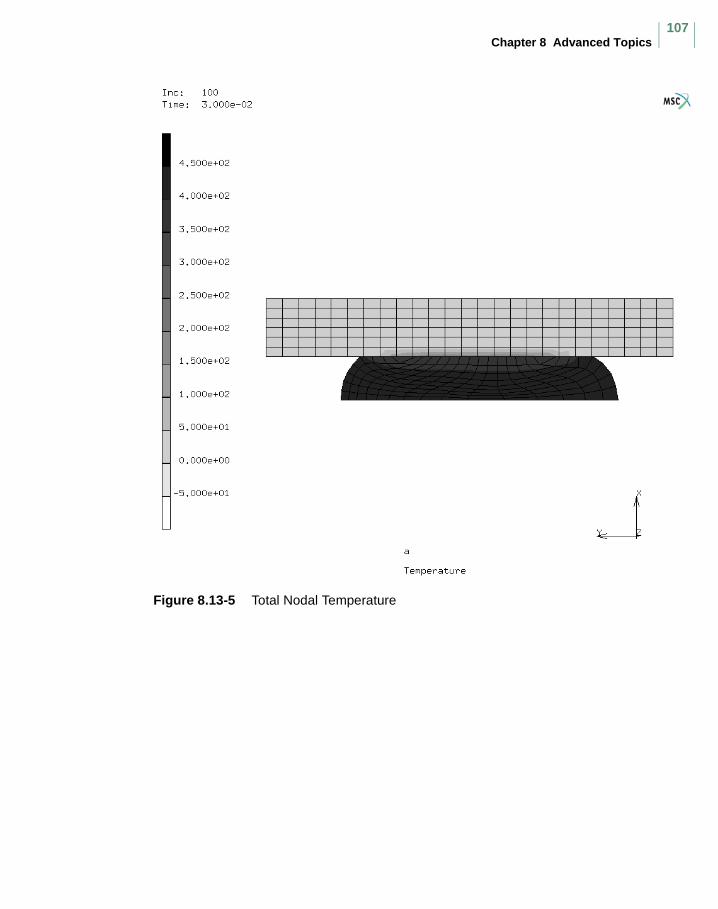
Chapter 8 Advanced Topics107
Figure 8.13-5 Total Nodal Temperature
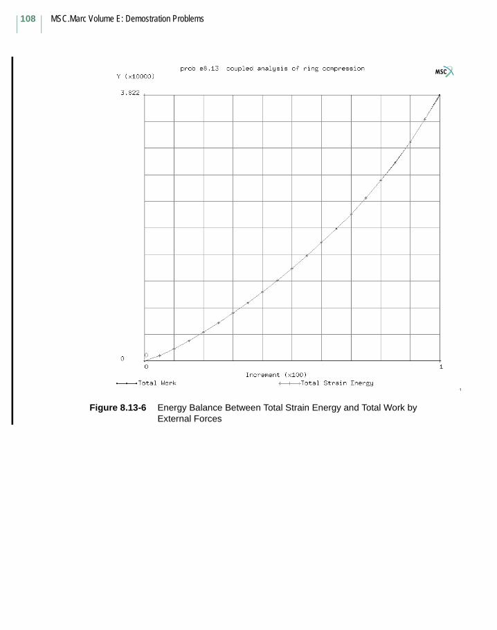
MSC.Marc Volume E: Demostration Problems
108
Figure 8.13-6 Energy Balance Between Total Strain Energy and Total Work by External Forces
Chapter 8 Advanced Topics109
8.23 3-D Magnetostatic Analysis of a CoilThis problem shows magnetostatic analysis capability using a 3-D element formulation in Marc. Since the potential to be solved is a new vector potential, the normal “heat transfer” approach cannot be used. Instead, an eight-noded magnetostatic element (type 109) is used for this analysis.
Parameters
The MAGNETO parameter is included to indicate a magnetostatic analysis.
Mesh Definition
One quarter of the coil is modeled using element type 109. The outside radius is 3.0 cm. Figure 8.23-1 shows the mesh and applied current.
Boundary Conditions
Along the y = 0 edge A1 = 0. Along the x = 0 edge A2 = 0. Along the outside radius A1 = A2 = 0. A3 = 0 everywhere to simulate a two-dimensional problem.
Material Properties
The magnetic permeability of all elements is set to 1000.0 Henry/cm.
Currents
A current running in the circumferential direction at a radius of 1 cm is applied. The point currents ranging in value from -0.951 amps to +0.951 amps are applied at nodes 111 to 120.
POST
The following variables are written to both a binary and a formatted post file:
141-143 Components of magnetic flux
144-146 Components of magnetic intensity
MSC.Marc Volume E: Demostration Problems
110
Results
The third component of the magnetic induction is shown as a function of the radius in Figure 8.23-2. You can observe that a steep gradient occurs about the ring of nodes to which the current is applied. In addition, the magnetization inside the coil cancels out with the magnetization outside the coil, as:
πrc2 (28650) / π(ro
2 – rc2) (-3560) = -1.006
where rc = 1, and ro = 3. Using the so called Biot-Savart equation we find for the magnetic induction inside the coil B = 31830, while from Figure 8.23-2 B = 28650. The difference is due to forcing A1 = A2 = 0 at the outside radius, while with the Biot-Savart equation the coil is in infinite space.
The vector potential A is shown in Figure 8.23-3.
Parameters, Options, and Subroutines Summary
Example e8x23.dat:
Example e8x23b.dat:
Parameters Model Definition Options History Definition Options
ELEMENT CONNECTIVITY CONTINUE
END COORDINATE STEADY STATE
MAGNETOSTATIC END OPTION
SIZING FIXED POTENTIAL
TITLE ISOTROPIC
POINT CURRENT
POST
Parameters Model Definition Options History Definition Options
ELEMENT CONNECTIVITY CONTINUE
END COORDINATE STEADY STATE
MAGNETOSTATIC DEFINE
SIZING END OPTION
TITLE FIXED POTENTIAL
ISOTROPIC
POINT CURRENT
POST
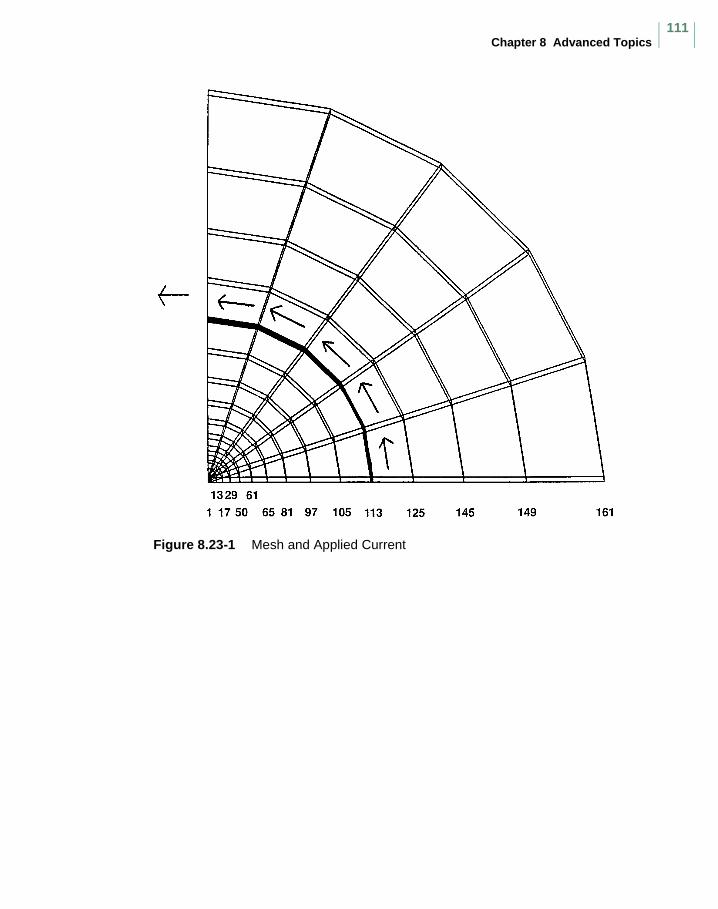
Chapter 8 Advanced Topics111
Figure 8.23-1 Mesh and Applied Current
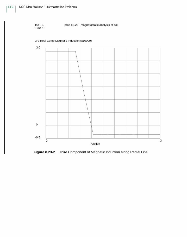
MSC.Marc Volume E: Demostration Problems
112
Figure 8.23-2 Third Component of Magnetic Induction along Radial Line
prob e8.23 magnetostatic analysis of coil
Position
3rd Real Comp Magnetic Induction (x10000)
Inc : 1Time : 0
3-0.5
0
0
3.0
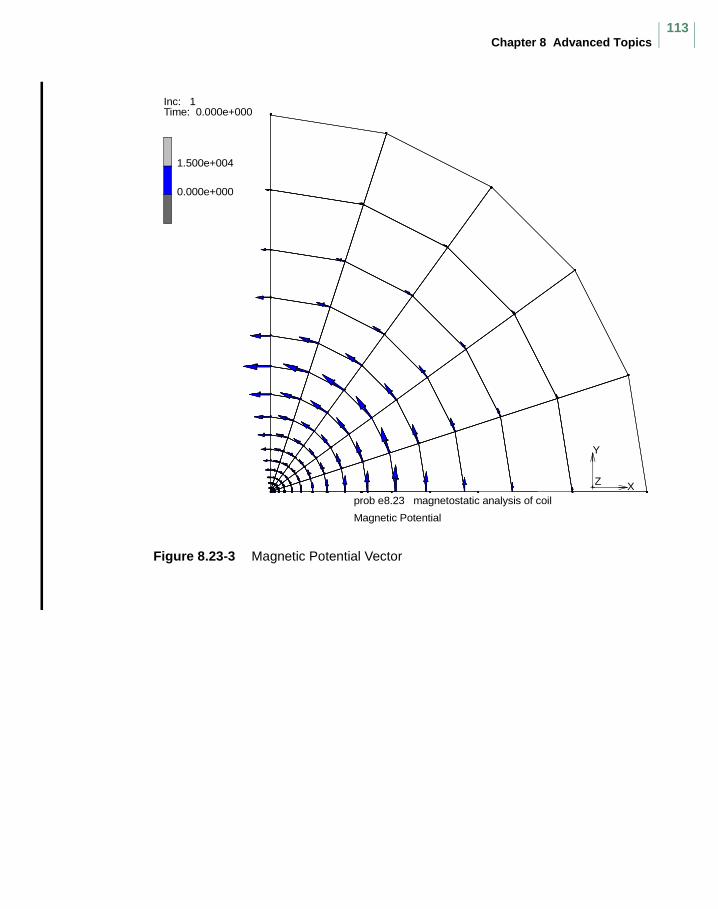
Chapter 8 Advanced Topics113
Figure 8.23-3 Magnetic Potential Vector
0.000e+000
1.500e+004
prob e8.23 magnetostatic analysis of coil
Magnetic Potential
Inc: 1Time: 0.000e+000
X
Y
Z
MSC.Marc Volume E: Demostration Problems
114
8.37 Interference Fit AnalysisThis example demonstrates the interference fit capabilities in Marc and the use of symmetry planes.
Element
Element type 11, a four node plane strain element, is used in this analysis. The model, as shown in Figure 8.37-1, consists of a 90° segment of two rings rotated by 45°. Ten elements (9° each) are used in the circumferential direction. The inner cylinder, with ri = 1 inch and r0 = 2 inches, has five elements through the radius. The outer cylinder, with ri = 2 inches and ro = 3 inches, has six elements. Two symmetry surfaces at 45° and 135° are used. To prevent any rigid body motion, a spring was placed between the two bodies. While this was not necessary in this problem, it is often a good idea.
Loading
The kinematic boundaries are specified using the symmetry surfaces. This problem is driven by the overclosure fit of 0.01 inch specified through the CONTACT TABLE option.
Material Properties
The material is a high strength steel with a Young’s modulus of 30 x 106 psi, a Poisson’s ratio of 0.3 and a yield stress of 50,000 psi. The material remains elastic in this analysis.
Contact
There are four bodies defined: the inner cylinder, outer cylinder, symmetry surface at θ = 135°, and symmetry surface at θ = 45°.
No friction exists on any surface. Note the flag set on the fourth data block to indicate that surface 3 and 4 are symmetry surfaces. The CONTACT TABLE option is used to indicate which bodies can potentially contact others and to specify the closure distance and the overclosure amount. The overclosure was set to 0.01 inch.
The SPLINE option is used to obtain a more accurate calculation of the surface normals than would have been otherwise.
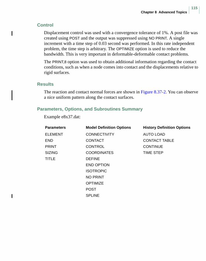
Chapter 8 Advanced Topics115
Control
Displacement control was used with a convergence tolerance of 1%. A post file was created using POST and the output was suppressed using NO PRINT. A single increment with a time step of 0.03 second was performed. In this rate independent problem, the time step is arbitrary. The OPTIMIZE option is used to reduce the bandwidth. This is very important in deformable-deformable contact problems.
The PRINT,8 option was used to obtain additional information regarding the contact conditions, such as when a node comes into contact and the displacements relative to rigid surfaces.
Results
The reaction and contact normal forces are shown in Figure 8.37-2. You can observe a nice uniform pattern along the contact surfaces.
Parameters, Options, and Subroutines Summary
Example e8x37.dat:
Parameters Model Definition Options History Definition Options
ELEMENT CONNECTIVITY AUTO LOAD
END CONTACT CONTACT TABLE
PRINT CONTROL CONTINUE
SIZING COORDINATES TIME STEP
TITLE DEFINE
END OPTION
ISOTROPIC
NO PRINT
OPTIMIZE
POST
SPLINE

MSC.Marc Volume E: Demostration Problems
116
Figure 8.37-1 Finite Element Mesh with Symmetry Surfaces
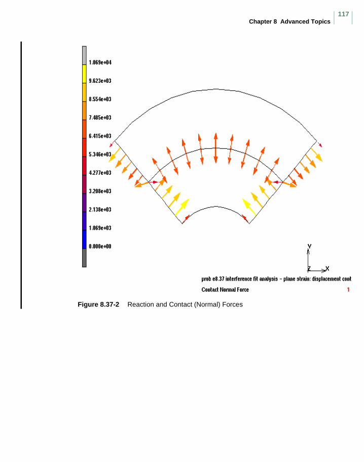
Chapter 8 Advanced Topics117
Figure 8.37-2 Reaction and Contact (Normal) Forces

MSC.Marc Volume E: Demostration Problems
118
8.55 Deep Drawing of Copper SheetThis example shows the deep drawing of a copper sheet. Shell elements are used to model the sheet. There are two data sets in this example. Data set e8x55a uses a velocity controlled punch. Data set e8x55b uses a load controlled punch. The effect of a blankholder is modeled using a fixed rigid surface at a small distance above the sheet.
Model
The initial model is shown in Figure 8.55-1. A 15° sector of the punch is used. The model consists of 79 elements and 121 nodes to model the sheet. There are five rigid bodies in the model, a punch, a lower die, two symmetry bodies, and a blankholder. In the case of data set e8x55b, an extra detached node (number 122) is associated with the rigid punch and a point load is applied to this node.
Element
The 4 noded thick shell element number 75 is used in this example to model the copper sheet.
Material Properties
The sheet is assumed to be isotropic with an elastic modulus of 17 x 106 psi and a
Poisson’s ratio of 0.33. The initial yield stress is assumed to be 1.08 x 10⁴ psi. The workhardening characteristics of the sheet are given by the WORK HARD model definition option.
Boundary Conditions
The boundary conditions for this problem are imposed using the CONTACT option.
Contact
There are 6 contact bodies in this problem. Contact body 1 is the deformable body representing the sheet. Body 2 is a rigid body representing the punch. In the case of data set e8x55a, the punch is a velocity controlled body moving at a speed of 3.2 in/s along the +x direction. For data set e8x55b, the punch is load controlled. Contact body 3 represents the lower die. Contact bodies 4 and 5 represent the symmetry surfaces in the problem and contact body 6 is the blankholder.
Chapter 8 Advanced Topics119
The stick-slip Coulomb friction model is used with a friction coefficient of 0.04. Default contact settings are used except that the iterative increment splitting and stress-based separation options are used.
Control
The convergence control is displacement based. The maximum allowed relative change in displacement increment is 0.05.
History Definition
For data set e8x55a, the punch is moved along the +x direction at a speed of 3.2 in/s for a further 99 increments. For data set e8x55b, a load of 3.08 lbs per increment is applied along the x direction for 79 increments.
Results
The final deformed geometry is shown in Figure 8.55-2 for data set e8x55a. The contours of total effective plastic strain are superimposed. The final deformed geometry is shown in Figure 8.55-3 for data set e8x55b. The contours of total effective plastic strain are superimposed. Figure 8.55-4 shows the total strain energy, the total work by external forces, and the contribution from friction.
Parameters, Options, and Subroutines Summary
Example e8x55a.dat and e8x55b.dat:
Parameters Model Definition Options History Definition Options
ALL POINTS CONNECTIVITY AUTO LOAD
ELEMENTS CONTACT CONTINUE
END CONTROL POINT LOAD
FINITE COORDINATES TIME STEP
LARGE DISP ISOTROPIC
SHELL SECT OPTIMIZE
SIZING POINT LOAD
TITLE WORK HARD
UPDATE
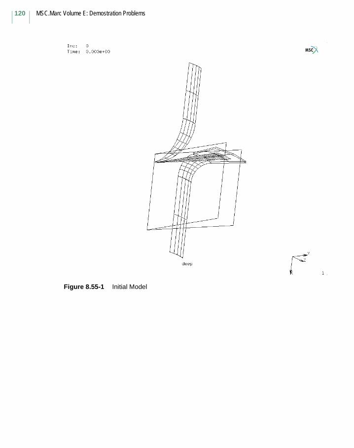
MSC.Marc Volume E: Demostration Problems
120
Figure 8.55-1 Initial Model
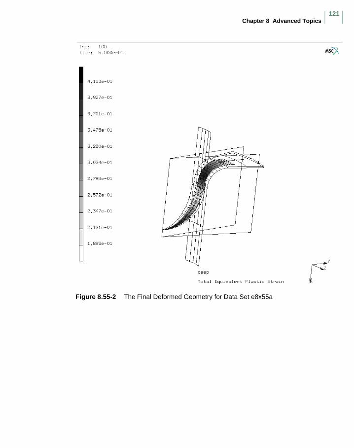
Chapter 8 Advanced Topics121
Figure 8.55-2 The Final Deformed Geometry for Data Set e8x55a
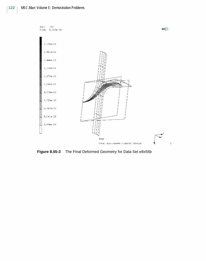
MSC.Marc Volume E: Demostration Problems
122
Figure 8.55-3 The Final Deformed Geometry for Data Set e8x55b
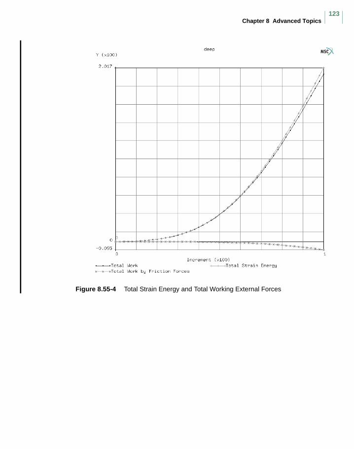
Chapter 8 Advanced Topics123
Figure 8.55-4 Total Strain Energy and Total Working External Forces
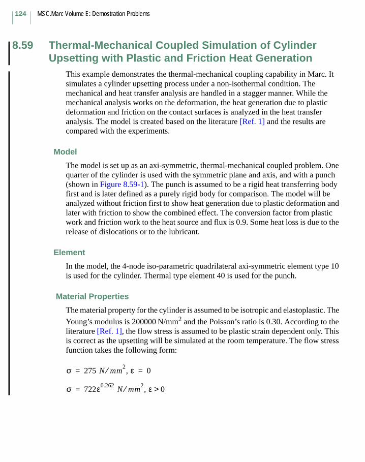
MSC.Marc Volume E: Demostration Problems
124
8.59 Thermal-Mechanical Coupled Simulation of Cylinder Upsetting with Plastic and Friction Heat Generation
This example demonstrates the thermal-mechanical coupling capability in Marc. It simulates a cylinder upsetting process under a non-isothermal condition. The mechanical and heat transfer analysis are handled in a stagger manner. While the mechanical analysis works on the deformation, the heat generation due to plastic deformation and friction on the contact surfaces is analyzed in the heat transfer analysis. The model is created based on the literature [Ref. 1] and the results are compared with the experiments.
Model
The model is set up as an axi-symmetric, thermal-mechanical coupled problem. One quarter of the cylinder is used with the symmetric plane and axis, and with a punch (shown in Figure 8.59-1). The punch is assumed to be a rigid heat transferring body first and is later defined as a purely rigid body for comparison. The model will be analyzed without friction first to show heat generation due to plastic deformation and later with friction to show the combined effect. The conversion factor from plastic work and friction work to the heat source and flux is 0.9. Some heat loss is due to the release of dislocations or to the lubricant.
Element
In the model, the 4-node iso-parametric quadrilateral axi-symmetric element type 10 is used for the cylinder. Thermal type element 40 is used for the punch.
Material Properties
The material property for the cylinder is assumed to be isotropic and elastoplastic. The
Young’s modulus is 200000 N/mm2 and the Poisson’s ratio is 0.30. According to the literature [Ref. 1], the flow stress is assumed to be plastic strain dependent only. This is correct as the upsetting will be simulated at the room temperature. The flow stress function takes the following form:
σ 275 N mm2⁄ , ε 0= =
σ 722ε0.262 N mm
2, ε 0>⁄=

Chapter 8 Advanced Topics125
The heat transfer properties are the thermal conductivity and the heat capacity:
For the cylinder:
For the punch:
Initial Conditions
Initial temperature is set at the room temperature 293K for both the cylinder and the punch.
Boundary Conditions
A fixed temperature at 293K is applied to the top surface of the punch (see Figure 8.59-2).
Contact
Contact bodies are:
Cylinder as the deformable bodyPunch as the rigid thermal body
The contact boundary conditions are:
1. Friction coefficient between the cylinder and the punch with shear friction law: 0.65
2. Heat transfer coefficient between cylinder and punch: 4 N/s/mm/K
3. Film coefficient to environment: 0.00295 N/s/mm/K
The motion of the punch represents a type of mechanical press and is defined as
where H is the current height of the cylinder. This motion is simulated through the use of the user subroutine u8x59.f.
k 36 N sK⁄=
ρc 3.77 N mm2K⁄=
k 19 N sK⁄=
ρc 3.77 N mm2K⁄=
ν 12* H 20–( )mm s⁄=
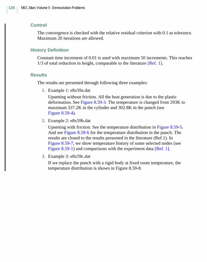
MSC.Marc Volume E: Demostration Problems
126
Control
The convergence is checked with the relative residual criterion with 0.1 as tolerance. Maximum 20 iterations are allowed.
History Definition
Constant time increment of 0.01 is used with maximum 50 increments. This reaches 1/3 of total reduction in height, comparable to the literature [Ref. 1].
Results
The results are presented through following three examples:
1. Example 1: e8x59a.dat
Upsetting without friction. All the heat generation is due to the plastic deformation. See Figure 8.59-3. The temperature is changed from 293K to maximum 337.2K in the cylinder and 302.8K in the punch (see Figure 8.59-4).
2. Example 2: e8x59b.dat
Upsetting with friction. See the temperature distribution in Figure 8.59-5. And see Figure 8.59-6 for the temperature distribution in the punch. The results are closed to the results presented in the literature (Ref.1). In Figure 8.59-7, we show temperature history of some selected nodes (see Figure 8.59-1) and comparisons with the experiment data [Ref. 1].
3. Example 3: e8x59c.dat
If we replace the punch with a rigid body at fixed room temperature, the temperature distribution is shown in Figure 8.59-8.
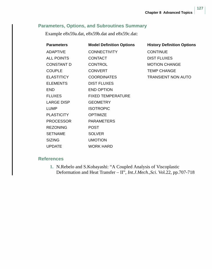
Chapter 8 Advanced Topics127
Parameters, Options, and Subroutines Summary
Example e8x59a.dat, e8x59b.dat and e8x59c.dat:
References
1. N.Rebelo and S.Kobayashi: “A Coupled Analysis of Viscoplastic Deformation and Heat Transfer – II”, Int.J.Mech.,Sci. Vol.22, pp.707-718
Parameters Model Definition Options History Definition Options
ADAPTIVE CONNECTIVITY CONTINUE
ALL POINTS CONTACT DIST FLUXES
CONSTANT D CONTROL MOTION CHANGE
COUPLE CONVERT TEMP CHANGE
ELASTITICY COORDINATES TRANSIENT NON AUTO
ELEMENTS DIST FLUXES
END END OPTION
FLUXES FIXED TEMPERATURE
LARGE DISP GEOMETRY
LUMP ISOTROPIC
PLASTICITY OPTIMIZE
PROCESSOR PARAMETERS
REZONING POST
SETNAME SOLVER
SIZING UMOTION
UPDATE WORK HARD
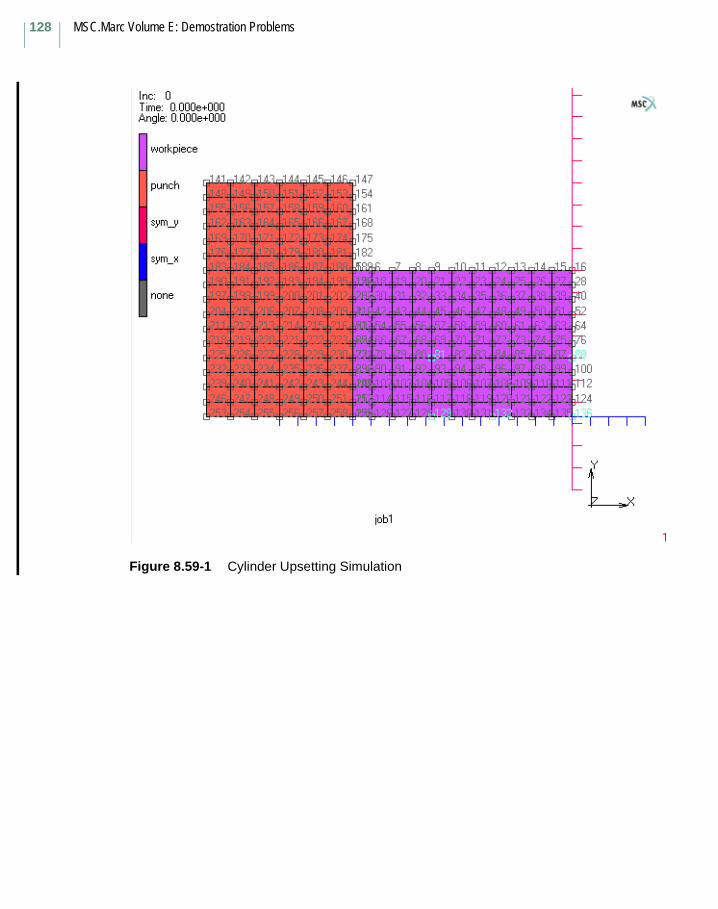
MSC.Marc Volume E: Demostration Problems
128
Figure 8.59-1 Cylinder Upsetting Simulation
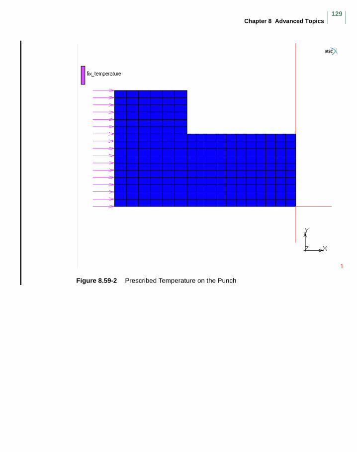
Chapter 8 Advanced Topics129
Figure 8.59-2 Prescribed Temperature on the Punch
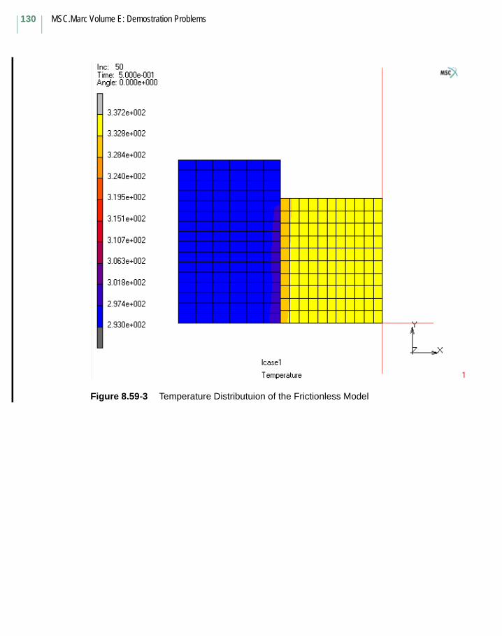
MSC.Marc Volume E: Demostration Problems
130
Figure 8.59-3 Temperature Distributuion of the Frictionless Model
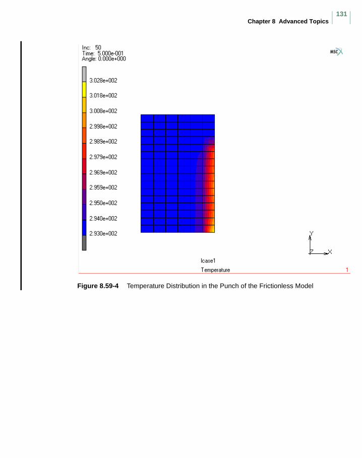
Chapter 8 Advanced Topics131
Figure 8.59-4 Temperature Distribution in the Punch of the Frictionless Model
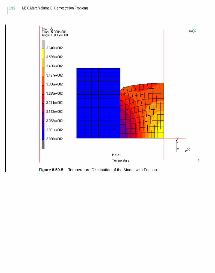
MSC.Marc Volume E: Demostration Problems
132
Figure 8.59-5 Temperature Distribution of the Model with Friction
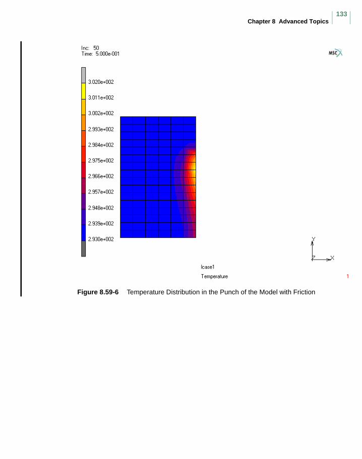
Chapter 8 Advanced Topics133
Figure 8.59-6 Temperature Distribution in the Punch of the Model with Friction
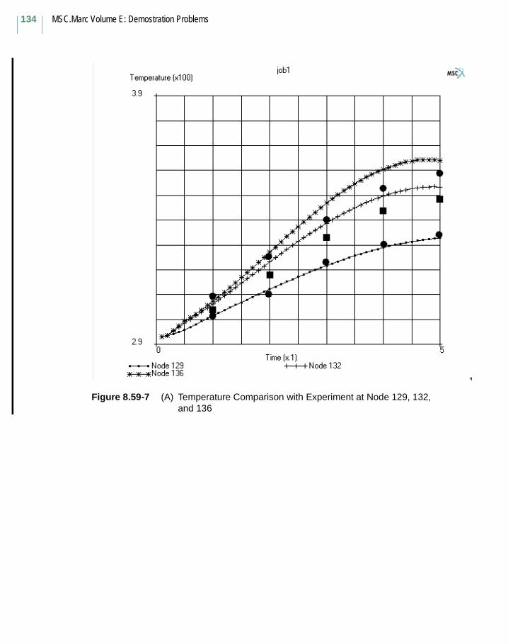
MSC.Marc Volume E: Demostration Problems
134
Figure 8.59-7 (A) Temperature Comparison with Experiment at Node 129, 132, and 136
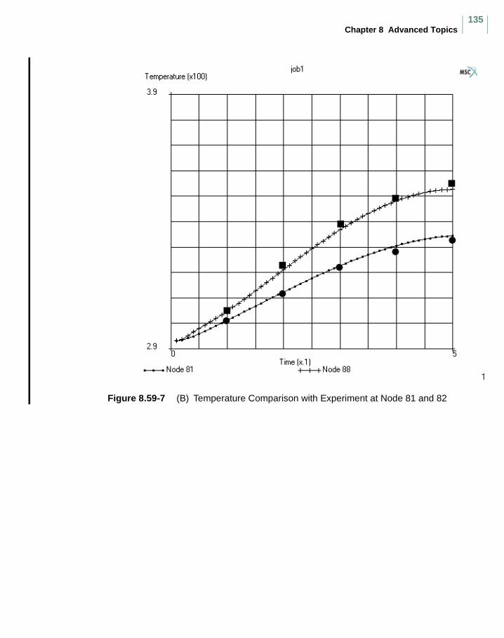
Chapter 8 Advanced Topics135
Figure 8.59-7 (B) Temperature Comparison with Experiment at Node 81 and 82
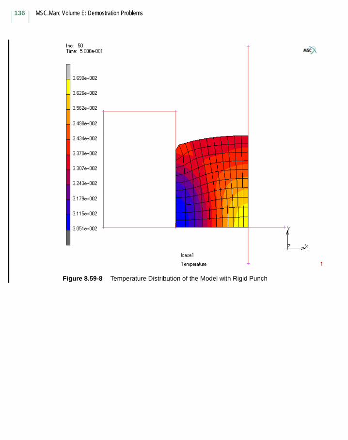
MSC.Marc Volume E: Demostration Problems
136
Figure 8.59-8 Temperature Distribution of the Model with Rigid Punch
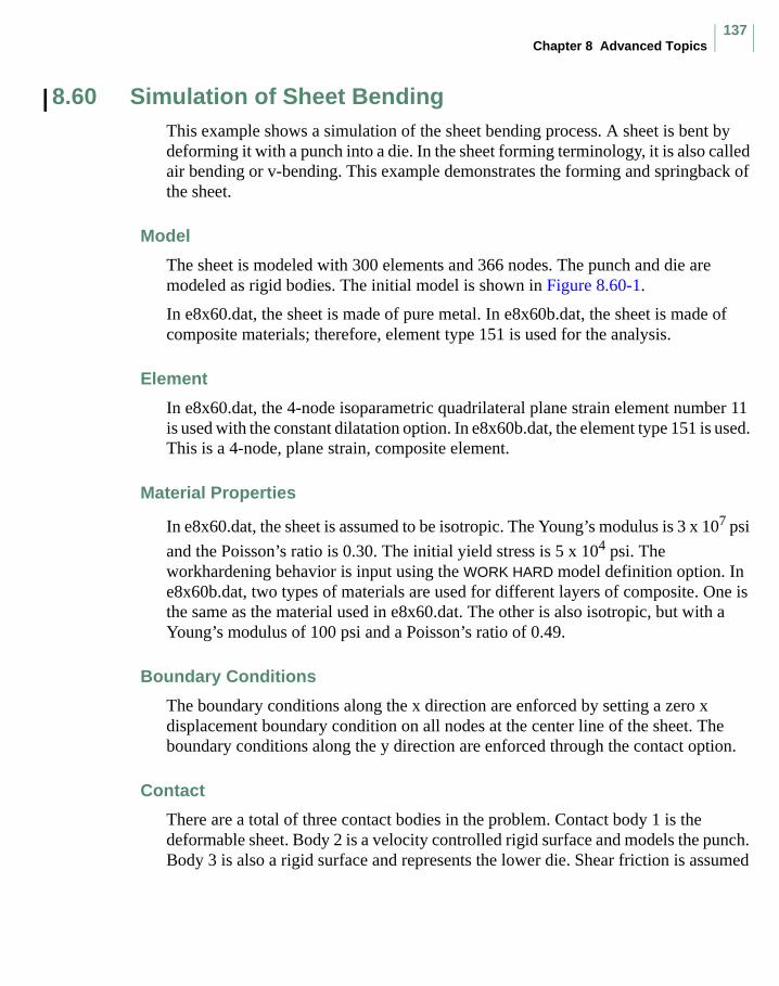
Chapter 8 Advanced Topics137
8.60 Simulation of Sheet BendingThis example shows a simulation of the sheet bending process. A sheet is bent by deforming it with a punch into a die. In the sheet forming terminology, it is also called air bending or v-bending. This example demonstrates the forming and springback of the sheet.
Model
The sheet is modeled with 300 elements and 366 nodes. The punch and die are modeled as rigid bodies. The initial model is shown in Figure 8.60-1.
In e8x60.dat, the sheet is made of pure metal. In e8x60b.dat, the sheet is made of composite materials; therefore, element type 151 is used for the analysis.
Element
In e8x60.dat, the 4-node isoparametric quadrilateral plane strain element number 11 is used with the constant dilatation option. In e8x60b.dat, the element type 151 is used. This is a 4-node, plane strain, composite element.
Material Properties
In e8x60.dat, the sheet is assumed to be isotropic. The Young’s modulus is 3 x 10⁷ psi
and the Poisson’s ratio is 0.30. The initial yield stress is 5 x 10⁴ psi. The workhardening behavior is input using the WORK HARD model definition option. In e8x60b.dat, two types of materials are used for different layers of composite. One is the same as the material used in e8x60.dat. The other is also isotropic, but with a Young’s modulus of 100 psi and a Poisson’s ratio of 0.49.
Boundary Conditions
The boundary conditions along the x direction are enforced by setting a zero x displacement boundary condition on all nodes at the center line of the sheet. The boundary conditions along the y direction are enforced through the contact option.
Contact
There are a total of three contact bodies in the problem. Contact body 1 is the deformable sheet. Body 2 is a velocity controlled rigid surface and models the punch. Body 3 is also a rigid surface and represents the lower die. Shear friction is assumed
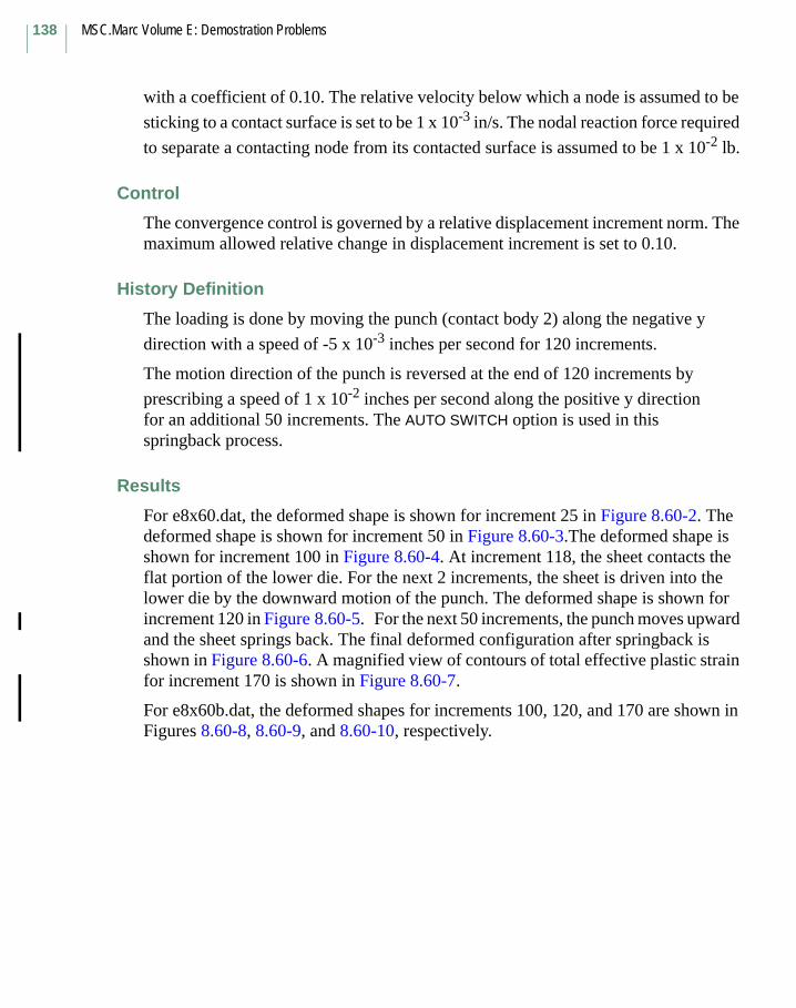
MSC.Marc Volume E: Demostration Problems
138
with a coefficient of 0.10. The relative velocity below which a node is assumed to be
sticking to a contact surface is set to be 1 x 10⁻³ in/s. The nodal reaction force required
to separate a contacting node from its contacted surface is assumed to be 1 x 10⁻² lb.
Control
The convergence control is governed by a relative displacement increment norm. The maximum allowed relative change in displacement increment is set to 0.10.
History Definition
The loading is done by moving the punch (contact body 2) along the negative y
direction with a speed of -5 x 10⁻³ inches per second for 120 increments.
The motion direction of the punch is reversed at the end of 120 increments by
prescribing a speed of 1 x 10⁻² inches per second along the positive y direction for an additional 50 increments. The AUTO SWITCH option is used in this springback process.
Results
For e8x60.dat, the deformed shape is shown for increment 25 in Figure 8.60-2. The deformed shape is shown for increment 50 in Figure 8.60-3.The deformed shape is shown for increment 100 in Figure 8.60-4. At increment 118, the sheet contacts the flat portion of the lower die. For the next 2 increments, the sheet is driven into the lower die by the downward motion of the punch. The deformed shape is shown for increment 120 in Figure 8.60-5. For the next 50 increments, the punch moves upward and the sheet springs back. The final deformed configuration after springback is shown in Figure 8.60-6. A magnified view of contours of total effective plastic strain for increment 170 is shown in Figure 8.60-7.
For e8x60b.dat, the deformed shapes for increments 100, 120, and 170 are shown in Figures 8.60-8, 8.60-9, and 8.60-10, respectively.

Chapter 8 Advanced Topics139
Parameters, Options, and Subroutines Summary
Example e8x60.dat:
Example e8x60b.dat:
Parameters Model Definition Options History Definition Options
ALL POINTS CONNECTIVITY AUTO LOAD
ELEMENTS CONTACT CONTINUE
END CONTROL MOTION CHANGE
PLASTICITY COORDINATES TIME STEP
SETNAME END OPTION
SIZING FIXED DISP
TITLE ISOTROPIC
SOLVER
WORK HARD
Parameters Model Definition Options History Definition Options
ALL POINTS COMPOSITE AUTO LOAD
ELEMENTS CONNECTIVITY CONTINUE
END CONTACT MOTION CHANGE
PLASTICITY CONTROL TIME STEP
SETNAME COORDINATES
SIZING END OPTION
TITLE FIXED DISP
ISOTROPIC
SOLVER
WORK HARD
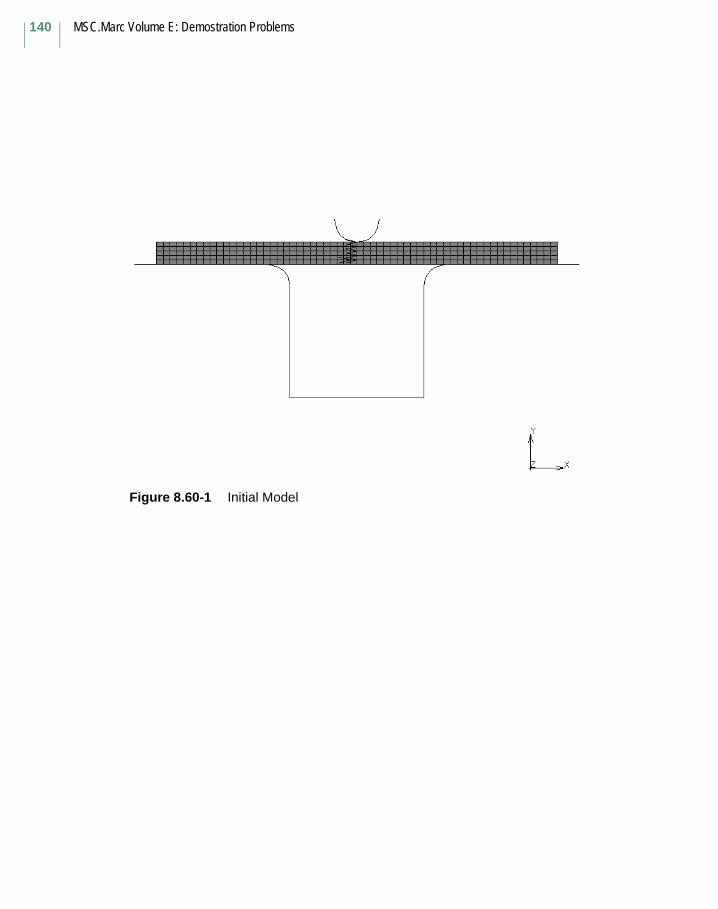
MSC.Marc Volume E: Demostration Problems
140
Figure 8.60-1 Initial Model
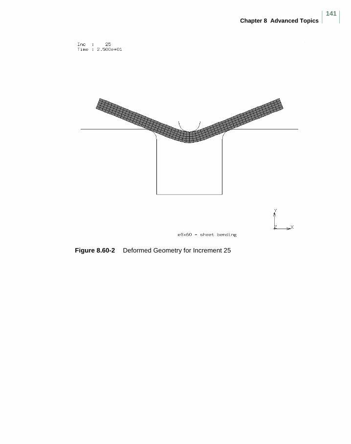
Chapter 8 Advanced Topics141
Figure 8.60-2 Deformed Geometry for Increment 25
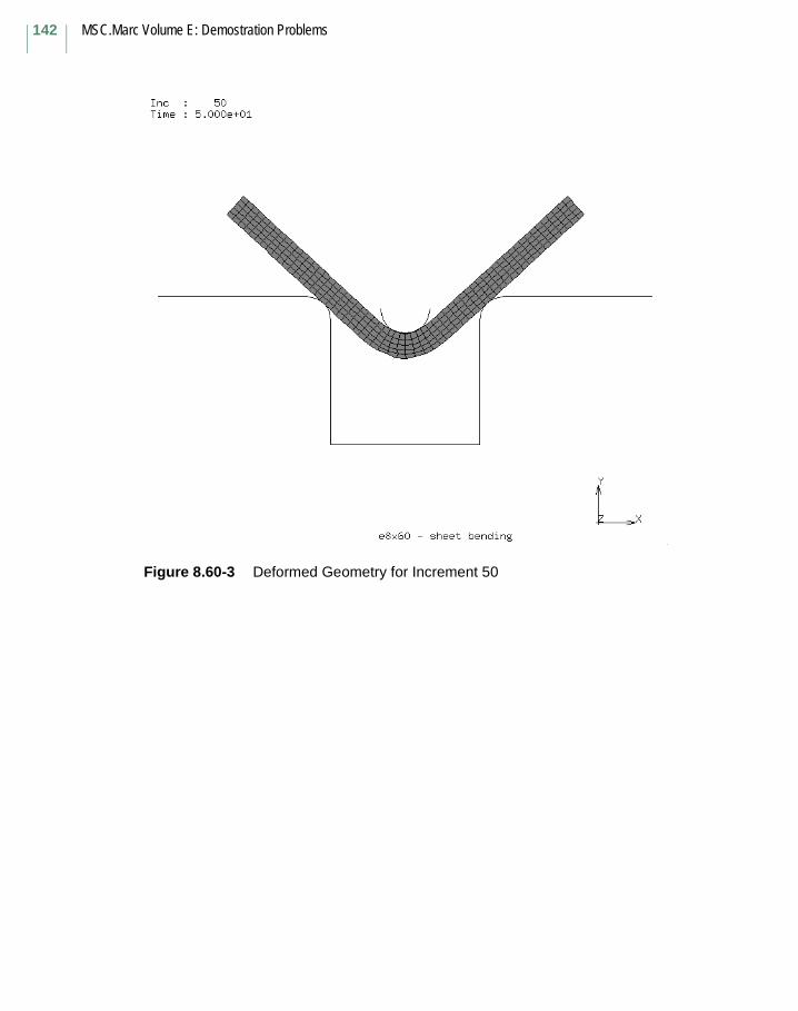
MSC.Marc Volume E: Demostration Problems
142
Figure 8.60-3 Deformed Geometry for Increment 50
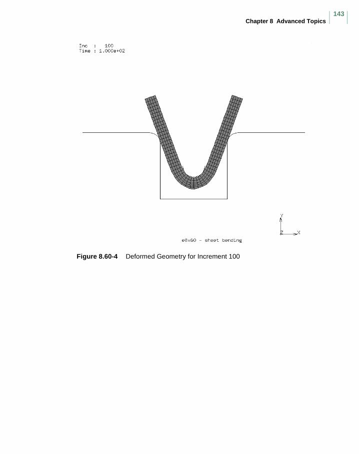
Chapter 8 Advanced Topics143
Figure 8.60-4 Deformed Geometry for Increment 100
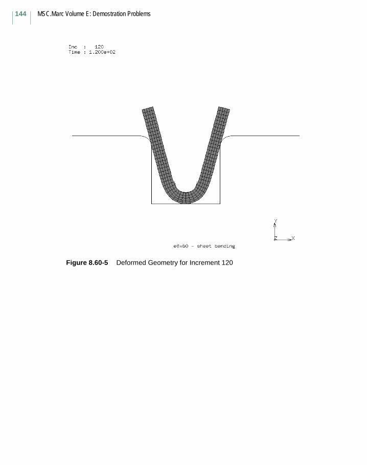
MSC.Marc Volume E: Demostration Problems
144
Figure 8.60-5 Deformed Geometry for Increment 120
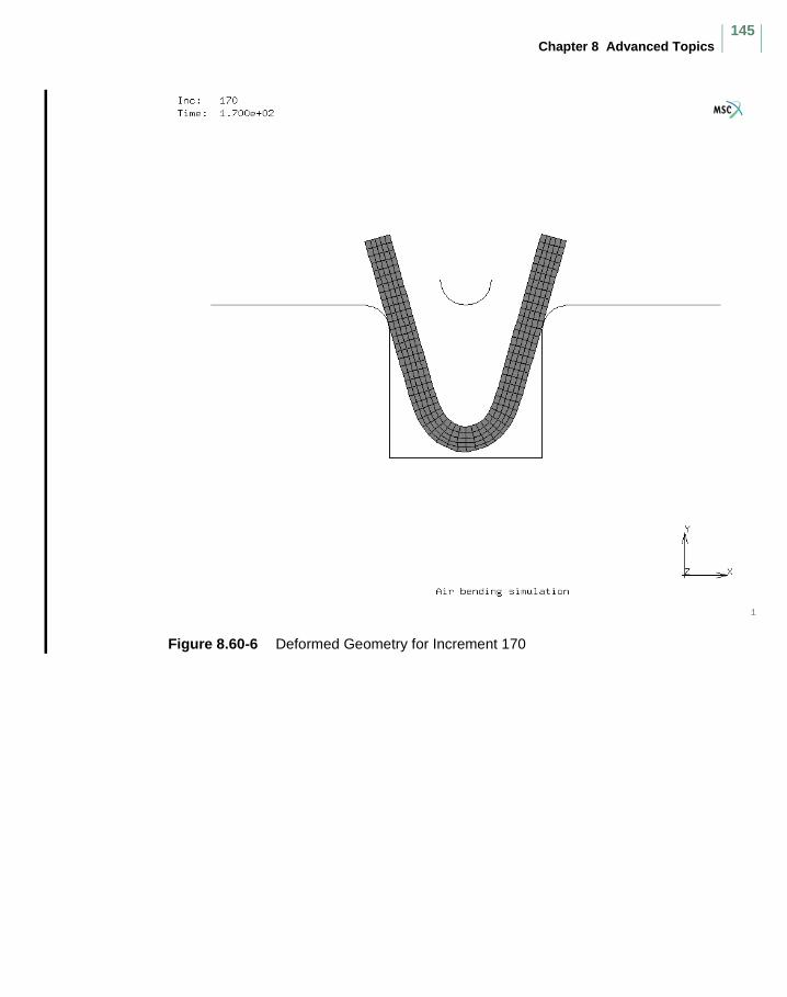
Chapter 8 Advanced Topics145
Figure 8.60-6 Deformed Geometry for Increment 170
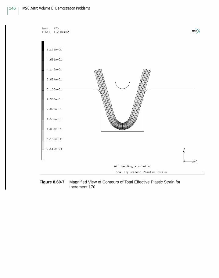
MSC.Marc Volume E: Demostration Problems
146
Figure 8.60-7 Magnified View of Contours of Total Effective Plastic Strain for Increment 170

Chapter 8 Advanced Topics147
Figure 8.60-8 Deformed Mesh at Increment 100 for e8x60b.dat
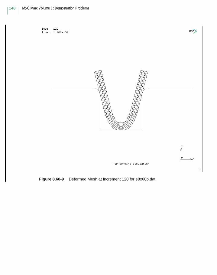
MSC.Marc Volume E: Demostration Problems
148
Figure 8.60-9 Deformed Mesh at Increment 120 for e8x60b.dat
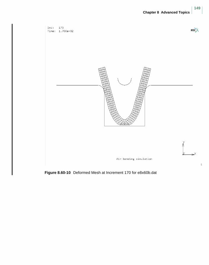
Chapter 8 Advanced Topics149
Figure 8.60-10 Deformed Mesh at Increment 170 for e8x60b.dat
MSC.Marc Volume E: Demostration Problems
150
8.61 Simulation of Rubber BushingA rubber bushing with an outer diameter of 10 cm and an inner diameter of 2 cm is considered. The length of the rubber bushing is 8 cm. Both outside and inside surfaces are glued to two steel tubes with corresponding diameters so that shape of the surfaces keeps unchanged during deformation. Two load sequences are applied. In the first step, a displacement of 2 cm along the symmetric axis is applied to the outside steel tube. During this load step, the deformation is purely axisymmetric. Afterwards, the outside steel tube moves 1 cm in the radial direction. In the second step, the problem becomes fully three-dimensional.
This example demonstrates the use of the data transfer capabilities of Marc from an axisymmetric analysis to an fully three-dimensional analysis.
Model
In axisymmetric analysis, the rubber bushing is modeled with 320 element and 371 nodes. The finite element mesh is shown in Figure 8.61-1. The model used in 3-D analysis is shown in Figure 8.61-2, which contains 3840 elements and 4823 nodes. Because of symmetry, only half of the rubber bushing is considered. The 3-D mesh in Figure 8.61-2 is an expansion of the deformed axisymmetric mesh in Figure 8.61-1.
Elements
The 4-node isoparametric quadrilateral axisymmetric element 10 is used in the axisymmetric run. The corresponding element type in 3-D run is 7 which is the 8-node isoparametric hexahedral element. In the analysis, both element types are based on mixed formulations and formulated on the deformed (updated) configuration. This is activated using ELASTICITY,2 parameter.
Material Properties
The rubber bushing is modeled using Mooney constitutive model. The material parameters are given as C1 = 8 N/cm and C2 = 2 N/cm.
Boundary Conditions and Load Definitions
Both outside and inside surfaces of the rubber bushing are glued to two steel tubes with corresponding diameters so that shape of the surfaces keeps unchanged during deformation. Two load sequences are applied. In the first step, a displacement of 2 cm along the symmetric axis is applied to the outside steel tube within 10 equal increments. During this load step, the deformation is purely axisymmetric and therefore an axisymmetric analysis is performed. Afterwards, the outside steel tube
Chapter 8 Advanced Topics151
moves 1 cm in the radial (Y) direction within 5 equal increments. In the second step, the problem becomes fully three-dimensional and therefore a 3-D analysis is performed.
Results
The deformed mesh and the distribution of equivalent von Mises stress at the end of axisymmetric analysis are shown in Figure 8.61-3. The corresponding results at increment 0 of the 3-D analysis is shown in Figure 8.61-4 which demonstrates the correctness of the axisymmetric to 3-D data transfer. Figure 8.61-5 contains the final deformed shape and the distribution of the equivalent von Mises stress.
Parameters, Options, and Subroutines Summary
Example e8x61a.dat:
Example e8x61b.dat:
Parameters Model Definition Options History Definition Options
ALL POINTS CONNECTIVITY AUTO LOADELASTICITY COORDINATES CONTINUEELEMENTS END OPTION CONTROLEND FIXED DISP DISP CHANGEPROCESSOR MOONEY TIME STEPSETNAME NO PRINT TITLESIZING OPTIMIZE TITLE POST
SOLVER
Parameters Model Definition Options History Definition Options
ALL POINTS AXITO3D AUTO LOADELASTICITY CONNECTIVITY CONTINUEELEMENTS COORDINATES CONTROLEND END OPTION DISP CHANGEPROCESSOR FIXED DISP TIME STEPSETNAME MOONEY TITLESIZING NO PRINTTITLE OPTIMIZE
POSTSOLVER

MSC.Marc Volume E: Demostration Problems
152
Figure 8.61-1 FE-Mesh for Axisymmetric Analysis
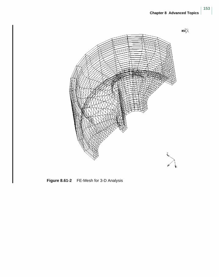
Chapter 8 Advanced Topics153
Figure 8.61-2 FE-Mesh for 3-D Analysis
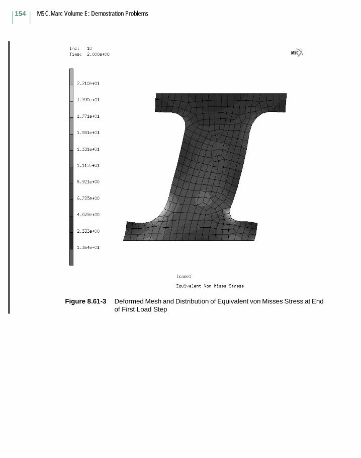
MSC.Marc Volume E: Demostration Problems
154
Figure 8.61-3 Deformed Mesh and Distribution of Equivalent von Misses Stress at End of First Load Step
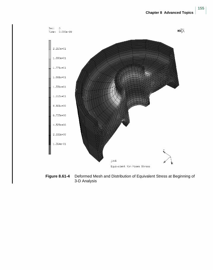
Chapter 8 Advanced Topics155
Figure 8.61-4 Deformed Mesh and Distribution of Equivalent Stress at Beginning of 3-D Analysis
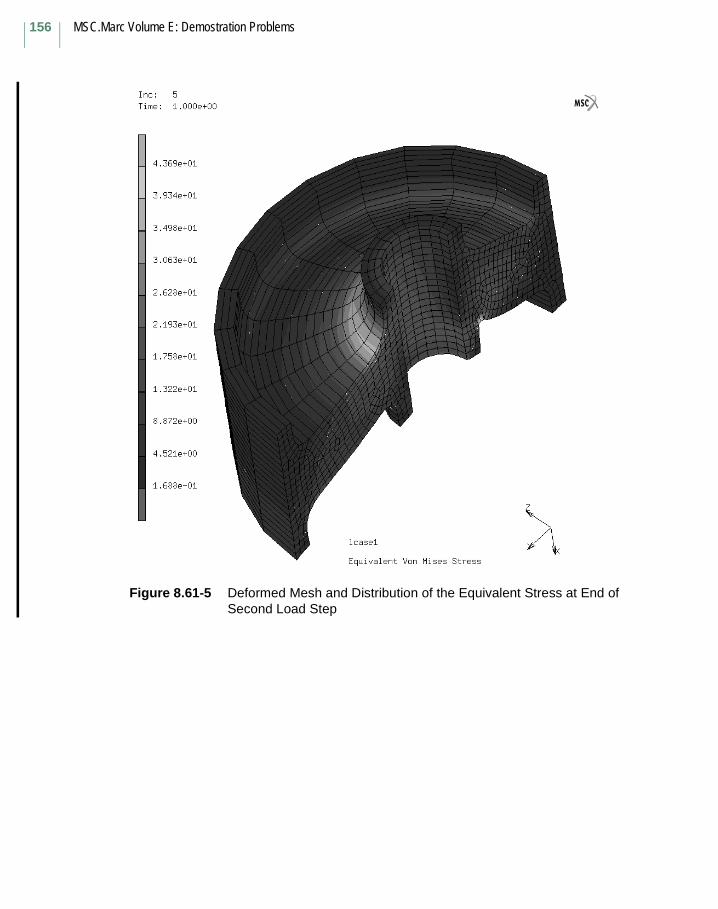
MSC.Marc Volume E: Demostration Problems
156
Figure 8.61-5 Deformed Mesh and Distribution of the Equivalent Stress at End of Second Load Step

Chapter 8 Advanced Topics157
8.63 Coupled Structural-acoustic AnalysisIn this example, a harmonic structural-acoustic analysis is performed on two spherical rooms, filled with air and separated by a rubber membrane (see Figure 8.63-1).
First, a harmonic analysis is performed on the stress-free structure. Then, a pre-stress is applied on the membrane, followed by a second harmonic analysis.
Elements
Element type 40, a 4-node axisymmetric isoparametric heat transfer element, is used to model the air. Element type 82, a 4-node axisymmetric isoparametric element for incompressible material, is used to model the membrane. Both element types use full integration.
Harmonic
The HARMONIC parameter is used since a frequency response analysis will be performed.
Acoustic
A harmonic acoustic analysis will be performed, which must be set by the ACOUSTIC parameter.
Mooney
The material properties of the elements corresponding to the membrane are given by
a Mooney constant and a density of .
Acoustic
The air in the spherical rooms is characterized by a bulk modulus of
and a density of .
Region
The REGION model definition option is used to indicate which elements correspond to the acoustic and which elements correspond to the solid part of the model.
C01 805×10 N m
2⁄= 1000kg m3⁄
1.55×10 N m
2⁄
1kg m3⁄
MSC.Marc Volume E: Demostration Problems
158
Fixed Displacement
The nodes at the outer radius of the membrane are fixed in both x- and y-direction.
Contact
Three contact bodies are defined. The first two bodies are acoustic bodies and contain the air in the spherical rooms. The third body is a deformable body and contains the elements of the rubber membrane (see Figure 8.63-2).
Exclude
The EXCLUDE option is used to avoid that nodes of the acoustic contact bodies will touch segments of the deformable contact body which have a normal vector being parallel to the y-axis.
No Print
The NO PRINT model definition option is used to suppress print out.
Post
The default nodal variables are put on the post file; no element variables are selected.
Harmonic
The external load is applied at a frequency range from 60 to 90 Hz, with a step size of 0.3 Hz.
Press Change
Node 63 is loaded by a nodal pressure with magnitude 10.
Displacement Change
A y-displacement of 0.001 is applied to the nodes at the outer radius of the membrane in order to introduce a pre-stressed state in the membrane, prior to a subsequent harmonic analysis.
Auto Load
The total displacement to get the pre-stress is applied in one step.

Chapter 8 Advanced Topics159
Time Step
Defining a time step during the pre-stressing of the membrane is necessary, because the CONTACT option is used.
Results
The pressure at node 168, located in the right room at the membrane as a function of the frequency is given in Figures 8.63-3 and 8.63-4, corresponding to the stress-free and the pre-stressed membrane, respectively. Due to the pre-stress, the peak value shifts to a higher frequency.
Parameters, Options, and Subroutines Summary
Example e8x63a.dat:
Parameters Model Definition Options History Definition Options
TITLE SOLVER TITLE
SIZING OPTIMIZE HARMONIC
ELEMENTS CONNECTIVITY PRESS CHANGE
PROCESSOR COORDINATES CONTROL
$NO LIST MOONEY AUTO LOAD
HARMONIC ACOUSTIC TIME STEP
ACOUSTIC REGION DISP CHANGE
END FIXED DISP CONTINUE
CONTACT
EXCLUDE
NO PRINT
POST
END OPTION
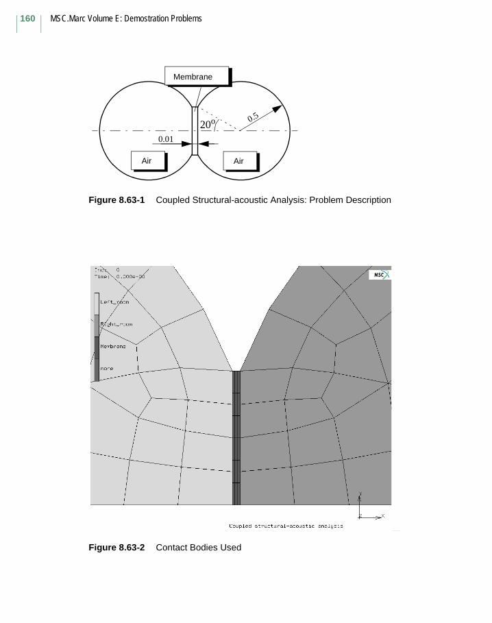
MSC.Marc Volume E: Demostration Problems
160
Figure 8.63-1 Coupled Structural-acoustic Analysis: Problem Description
Figure 8.63-2 Contact Bodies Used
20o 0.5
0.01
Air Air
Membrane
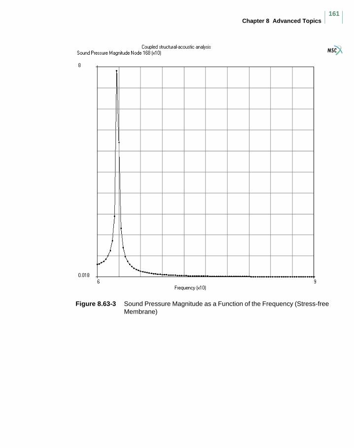
Chapter 8 Advanced Topics161
Figure 8.63-3 Sound Pressure Magnitude as a Function of the Frequency (Stress-free Membrane)
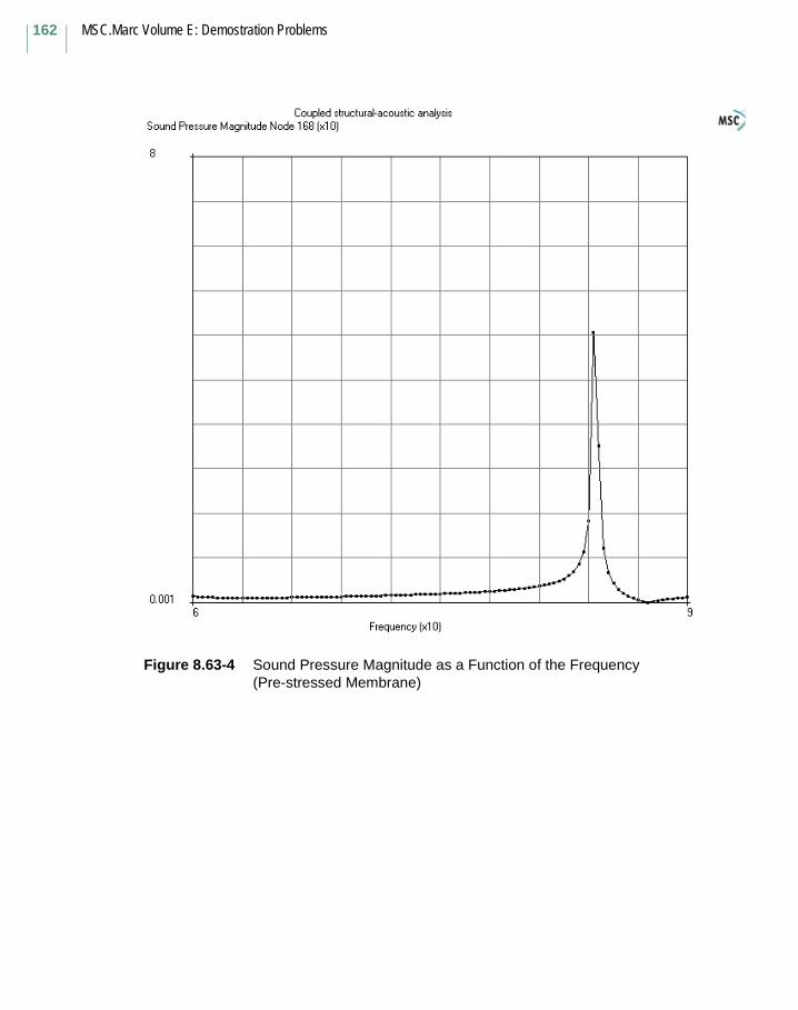
MSC.Marc Volume E: Demostration Problems
162
Figure 8.63-4 Sound Pressure Magnitude as a Function of the Frequency (Pre-stressed Membrane)
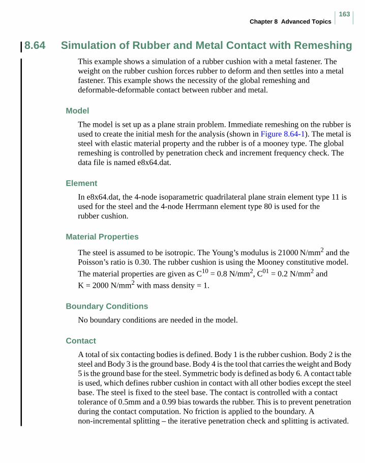
Chapter 8 Advanced Topics163
8.64 Simulation of Rubber and Metal Contact with RemeshingThis example shows a simulation of a rubber cushion with a metal fastener. The weight on the rubber cushion forces rubber to deform and then settles into a metal fastener. This example shows the necessity of the global remeshing and deformable-deformable contact between rubber and metal.
Model
The model is set up as a plane strain problem. Immediate remeshing on the rubber is used to create the initial mesh for the analysis (shown in Figure 8.64-1). The metal is steel with elastic material property and the rubber is of a mooney type. The global remeshing is controlled by penetration check and increment frequency check. The data file is named e8x64.dat.
Element
In e8x64.dat, the 4-node isoparametric quadrilateral plane strain element type 11 is used for the steel and the 4-node Herrmann element type 80 is used for the rubber cushion.
Material Properties
The steel is assumed to be isotropic. The Young’s modulus is 21000 N/mm2 and the Poisson’s ratio is 0.30. The rubber cushion is using the Mooney constitutive model.
The material properties are given as C10 = 0.8 N/mm2, C01 = 0.2 N/mm2 and
K = 2000 N/mm2 with mass density = 1.
Boundary Conditions
No boundary conditions are needed in the model.
Contact
A total of six contacting bodies is defined. Body 1 is the rubber cushion. Body 2 is the steel and Body 3 is the ground base. Body 4 is the tool that carries the weight and Body 5 is the ground base for the steel. Symmetric body is defined as body 6. A contact table is used, which defines rubber cushion in contact with all other bodies except the steel base. The steel is fixed to the steel base. The contact is controlled with a contact tolerance of 0.5mm and a 0.99 bias towards the rubber. This is to prevent penetration during the contact computation. No friction is applied to the boundary. A non-incremental splitting – the iterative penetration check and splitting is activated.
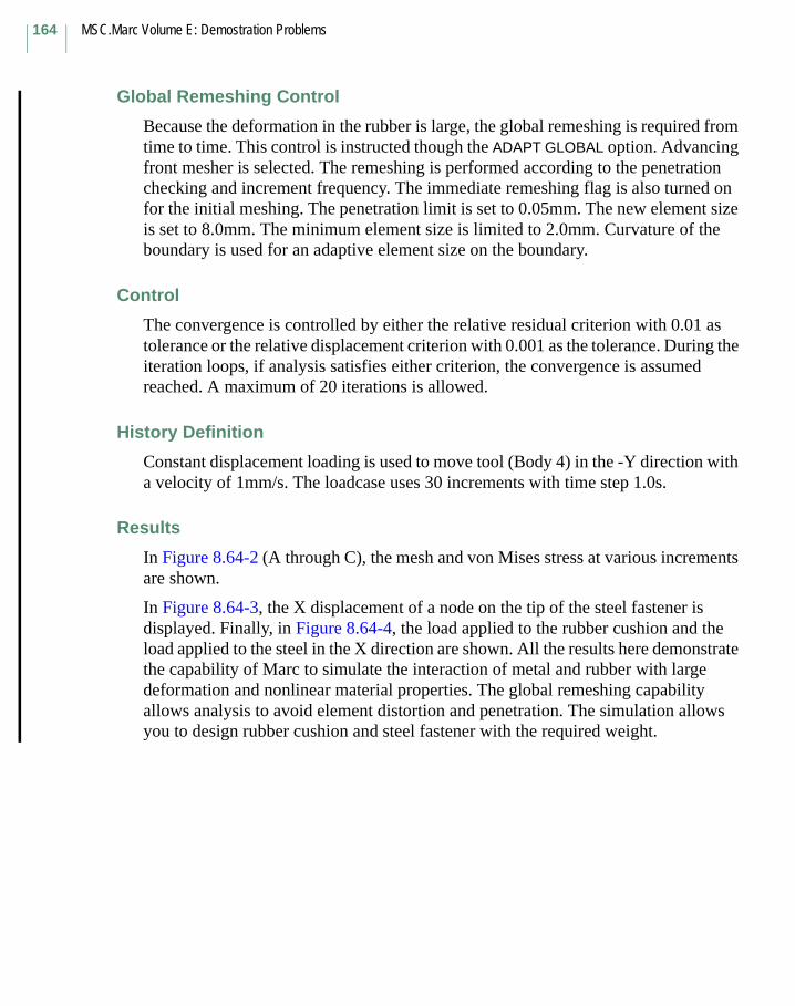
MSC.Marc Volume E: Demostration Problems
164
Global Remeshing Control
Because the deformation in the rubber is large, the global remeshing is required from time to time. This control is instructed though the ADAPT GLOBAL option. Advancing front mesher is selected. The remeshing is performed according to the penetration checking and increment frequency. The immediate remeshing flag is also turned on for the initial meshing. The penetration limit is set to 0.05mm. The new element size is set to 8.0mm. The minimum element size is limited to 2.0mm. Curvature of the boundary is used for an adaptive element size on the boundary.
Control
The convergence is controlled by either the relative residual criterion with 0.01 as tolerance or the relative displacement criterion with 0.001 as the tolerance. During the iteration loops, if analysis satisfies either criterion, the convergence is assumed reached. A maximum of 20 iterations is allowed.
History Definition
Constant displacement loading is used to move tool (Body 4) in the -Y direction with a velocity of 1mm/s. The loadcase uses 30 increments with time step 1.0s.
Results
In Figure 8.64-2 (A through C), the mesh and von Mises stress at various increments are shown.
In Figure 8.64-3, the X displacement of a node on the tip of the steel fastener is displayed. Finally, in Figure 8.64-4, the load applied to the rubber cushion and the load applied to the steel in the X direction are shown. All the results here demonstrate the capability of Marc to simulate the interaction of metal and rubber with large deformation and nonlinear material properties. The global remeshing capability allows analysis to avoid element distortion and penetration. The simulation allows you to design rubber cushion and steel fastener with the required weight.

Chapter 8 Advanced Topics165
Parameters, Options, and Subroutines Summary
Example e8x64.dat:
Parameters Model Definition Options History Definition Options
ALL POINTS CONNECTIVITY AUTO LOAD
ELEMENTS CONTACT CONTINUE
END CONTROL MOTION CHANGE
PLASTICITY COORDINATES TIME STEP
SETNAME END OPTION CONTACT TABLE
SIZING MOONEY
ELASTICITY ISOTROPIC
REZONING CONTACT TABLE
ADAPTIVE GEOMETRY
PROCESSOR SOLVER
OPTIMIZE
PARAMETERS
ADAPT GLOBAL
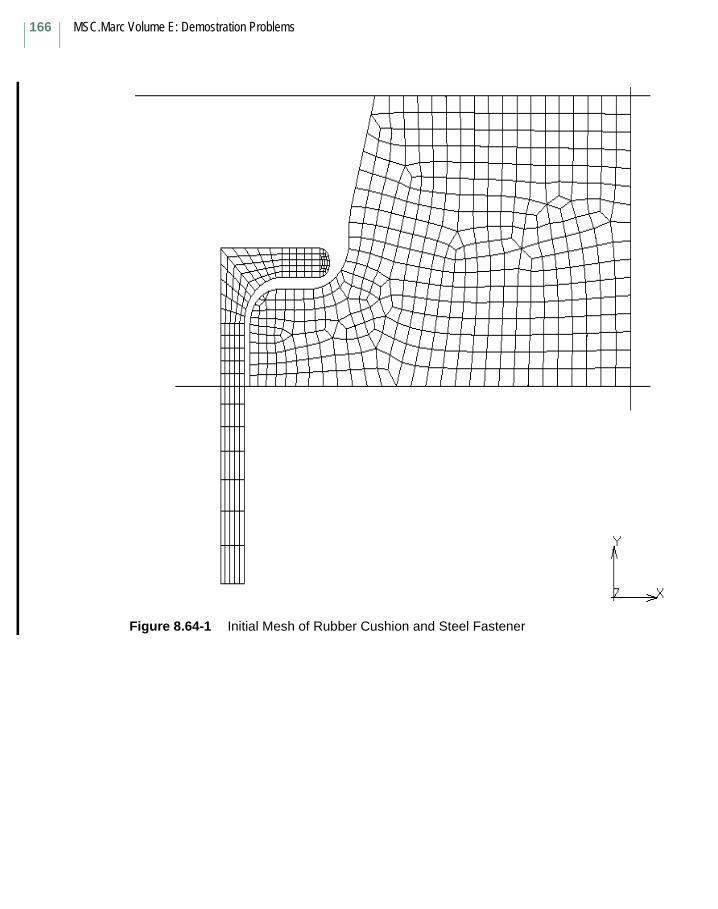
MSC.Marc Volume E: Demostration Problems
166
Figure 8.64-1 Initial Mesh of Rubber Cushion and Steel Fastener
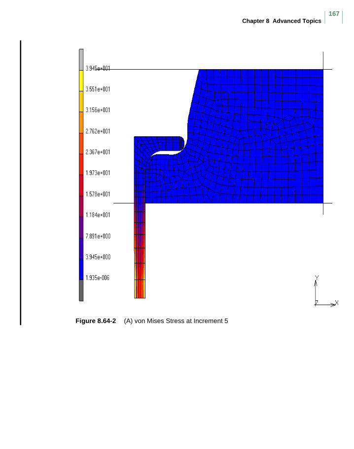
Chapter 8 Advanced Topics167
Figure 8.64-2 (A) von Mises Stress at Increment 5
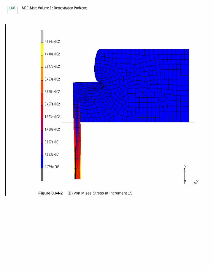
MSC.Marc Volume E: Demostration Problems
168
Figure 8.64-2 (B) von Mises Stress at Increment 15
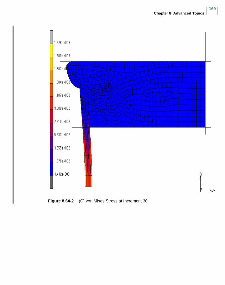
Chapter 8 Advanced Topics169
Figure 8.64-2 (C) von Mises Stress at Increment 30
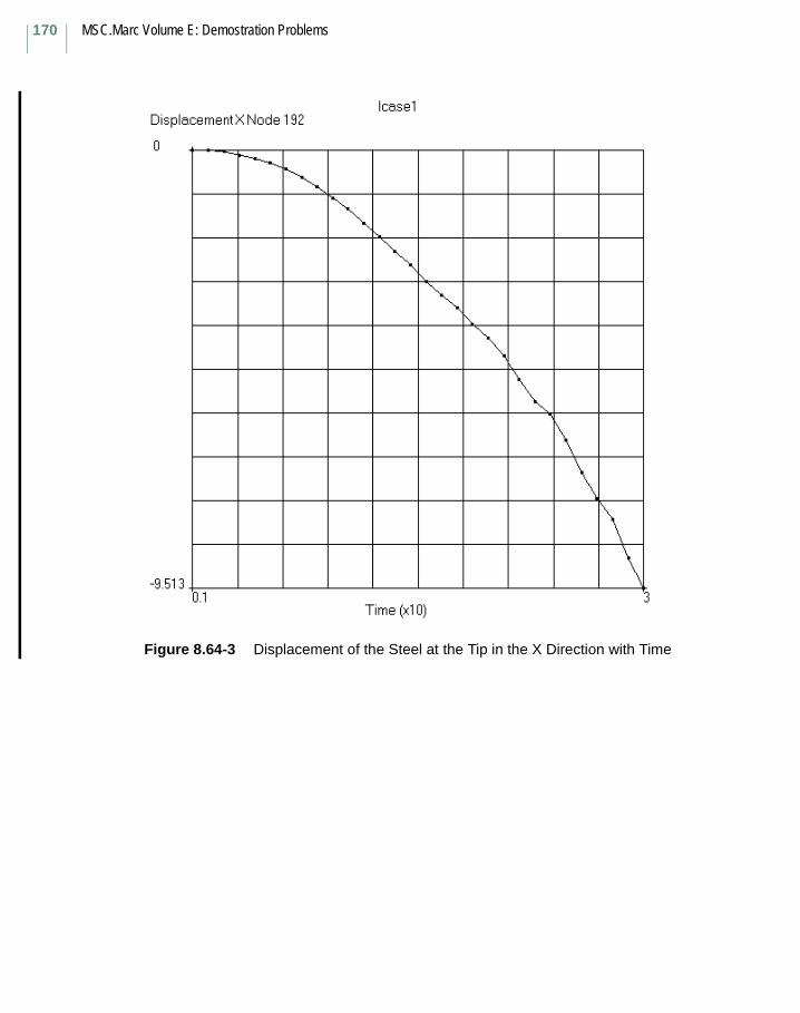
MSC.Marc Volume E: Demostration Problems
170
Figure 8.64-3 Displacement of the Steel at the Tip in the X Direction with Time
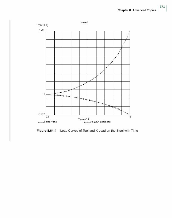
Chapter 8 Advanced Topics171
Figure 8.64-4 Load Curves of Tool and X Load on the Steel with Time

MSC.Marc Volume E: Demostration Problems
172
8.65 Pipe-nozzle Connection with a Rubber SealIn this example, a pipe is moved on a nozzle and a rubber seal between the pipe and the nozzle is used to avoid leakage (see Figure 8.65-1). The CONTACT TABLE option is used to automatically determine the proper order in which the search for contact will be performed
Figure 8.65-1 Pipe-nozzle connection with a rubber seal: problem description (units: mm)
The pipe is moved in the left-hand side direction over a distance . The nozzle is assumed to be fully clamped at the left edge.
Elements
Element type 10, a 4-node axisymmetric isoparametric element with full integration, is used to model both the steel nozzle and pipe as well as the rubber seal. The element mesh is shown in Figure 8.65-2. Notice that the nozzle and the pipe have been meshed in two separate regions, which will be glued together using the CONTACT TABLE option.
Seal 35 55 8010
0
80 112
105 12
5
7090
2025R=5
R=5
u=75
10
Nozzle
110
50
90 Pipe
u 75 mm=

Chapter 8 Advanced Topics173
Figure 8.65-2 Finite element mesh and contact bodies
Elasticity
The ELASTICITY parameter option is used to indicate that the elasticity procedure used will be based on the Updated Lagrange approach.
Mooney
The material properties of the elements corresponding to the seal are given by
Mooney constants and .
Isotropic
Both the nozzle and pipe are modeled using an isotropic material with Young’s
modulus and Poisson’s ratio
Fixed disp
The nodes on the left-hand side of the nozzle are fixed in both x- and y-direction, where the nodes in the right-hand side of the modeled part of the pipe will be moved in the left-hand side direction.
Contact
Five contact bodies are defined. The first two bodies build up the nozzle, the third body corresponds to the seal, the fourth and fifth body build up the pipe (see also Figure 8.65-2). Friction will be neglected.
Body 1 Body 4
Body 3
Body 4 Body 5
C01 0.8 N mm2⁄= C10 0.2 N mm
2⁄=
E 2.05×10 N mm
2⁄= υ 0.3=

MSC.Marc Volume E: Demostration Problems
174
Spline
The SPLINE option is used to get a smooth boundary description of the curved part of the nozzle. So it is only invoked for the second contact body. The nodes where the normal vector to the boundary of this body is discontinuous are given as input to the program.
Contact table
The CONTACT TABLE option is used here for various purposes. First, only a limited number of contact body pairs need to be considered; this reduces the computational time. Second, glued contact is activated between the two bodies defining the nozzle (bodies 1 and 2) and the two bodies defining the pipe (bodies 4 and 5). Third, the order in which the search for contact will be performed has to be determined by the program and will be based on the rule that for a particular contact body pair, nodes of the body with the smallest element edge length at the boundary will be checked with respect to the other body.
No print
The NO PRINT model definition option is used to suppress print out.
Post
The default nodal variables will be put on the post file; the element variable selected is the Cauchy stress tensor.
Control
The default control parameters are used. An incremental solution is accepted if the ratio of the maximum residual force component and the maximum reaction force component is less than 0.1. A full Newton-Raphson procedure is applied and the maximum number of iterations per increment is 10.
Auto step
Automatic load incrementation based on the AUTO STEP option is selected. The initial time increment is 0.025 times the total time. The desired number of recycles per increment is set to 3 and the load incrementation factor is set to 1.2.

Chapter 8 Advanced Topics175
Disp change
The nodes on the left-hand side of the nozzle are completely fixed, where the nodes on the right-hand side of the pipe are moved in the negative x-direction over a distance of 75.
Results
The equivalent Cauchy stress is the final deformed configuration is given in Figure 8.65-3. Figure 8.65-4 shows the relation between the increment number and the time. An increasing time step resulting from the AUTO STEP option can be observed.
Summary of Options Used
Parameter Options Model Definition Options History Definition Options
TITLE SOLVER TITLE
SIZING OPTIMIZE CONTROL
ELEMENTS CONNECTIVITY AUTO STEP
PROCESSOR COORDINATES DISP CHANGE
$NO LIST MOONEY CONTINUE
ELASTICITY ISOTROPIC
END FIXED DISP
CONTACT
SPLINE
CONTACT TABLE
NO PRINT
POST
END OPTION
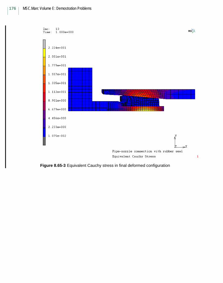
MSC.Marc Volume E: Demostration Problems
176
Figure 8.65-3 Equivalent Cauchy stress in final deformed configuration
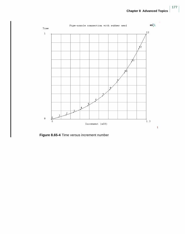
Chapter 8 Advanced Topics177
Figure 8.65-4 Time versus increment number
MSC.Marc Volume E: Demostration Problems
178
8.66 A Block Sliding over a Flat Surface This example shows how a block, with an initial velocity of 4.905, slides on a rigid surface. This block sliding process requires dynamic analysis with considerations of contact, friction, heat transfer, dampings, and the conversion of friction energy into thermal energy. The energy changes with the sliding of the block are demonstrated.
Model
The block is modeled with 8 brick elements. In e8x66.dat, the block is pure metal. The sliding surface is modeled as rigid body. The initial model is shown in Figure 8.66-1.
Element
Element type 7 is used for the analysis.
Material Properties
In e8x66.dat, the block is assumed to be isotropic for both mechanical and thermal
analysis. The Young’s modulus is 2.1 x 10¹¹ and the Poisson’s ratio is 0.3. Mass density is given as 7854 for both dynamic and heat transfer analysis. The conductivity is 60.5 and the specific heat is set as 434. Only proportional mass damping is applied with a ratio of 0.3. Lumped mass matrix is used in the example. The conversion rate for friction work into thermal energy is given as 1.0.
Boundary Conditions
The boundary conditions along the x-direction are enforced by setting a y-displacement boundary condition of zero on all nodes. In order to keep the block sliding on the surface, a body force of -9.81 is applied to each element along the z-direction. The block is given an initial velocity of 4.905 along the x-direction and an initial temperature of 0 at the beginning of the sliding process.
Contact
There is a total of two contact bodies in the problem. Contact Body 1 is the deformable block. Body 2 is a velocity controlled rigid surface, but not moving in space. Coulomb friction is applied with a friction co-efficient of 0.5 based on nodal forces. The relative sliding velocity for friction below which a node is assumed to be sticking to a contact surface is set at 0.1. The nodal reaction force required to separate a contacting node
from its contacted surface is assumed to be 1 x 10¹¹.
Chapter 8 Advanced Topics179
Control
The convergence control is governed by a relative displacement increment norm. The maximum allowed relative change in displacement is set to 0.10. For the heat transfer part, the maximum temperature change is set to be 20.
History Definition
The process is analyzed by coupled dynamics with SSH method (DYNAMIC,6). The total time of the process is 2 which takes 50 increments.
Results
At the end of increment 50, the equivalent von Mises stress and temperature are shown in Figures 8.66-2 and 8.66-3, respectively. Figure 8.66-4 shows the energy changes from increment 0 to increment 50. It shows that the kinetic energy is eventually transferred into damping energy and friction energy. The strain energy is very small. Figure 8.66-5 shows the conversion of friction work into thermal energy. It also demonstrates that the friction forces contribute, to a high degree, part of the work done by external force in this example.
Parameters, Options, and Subroutines Summary
Example e8x66.dat:
Parameter Model Definition Option History Definition Options
ALL POINTS CONNECTIVITY CONTINUE
COUPLED CONTACT CONTROL
DIST LOADS CONTROL DIST LOADS
DYNAMIC CONVERT DYNAMIC CHANGE
ELEMENTS COORDINATES MOTION CHANGE
END DAMPING PARAMETERS
EXTENDED DIST LOADS
LARGE DISP END OPTION
LUMP FIXED DISP
PROCESSOR INITIAL TEMP
SETNAME INITIAL VEL
SIZING NO PRINT
TITLE OPTIMIZE
PARAMETERS
POST
SOLVER
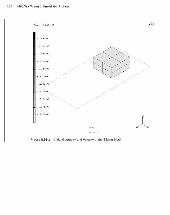
MSC.Marc Volume E: Demostration Problems
180
Figure 8.66-1 Initial Geometry and Velocity of the Sliding Block
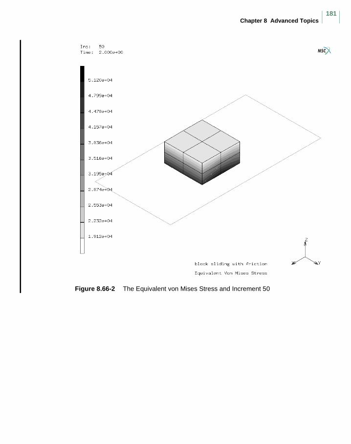
Chapter 8 Advanced Topics181
Figure 8.66-2 The Equivalent von Mises Stress and Increment 50
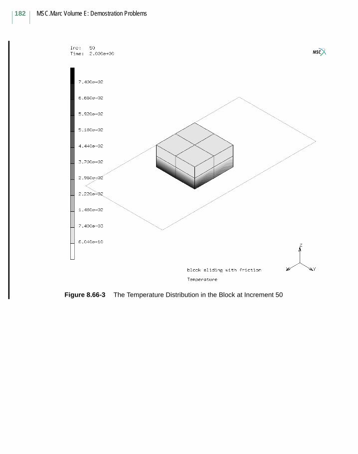
MSC.Marc Volume E: Demostration Problems
182
Figure 8.66-3 The Temperature Distribution in the Block at Increment 50
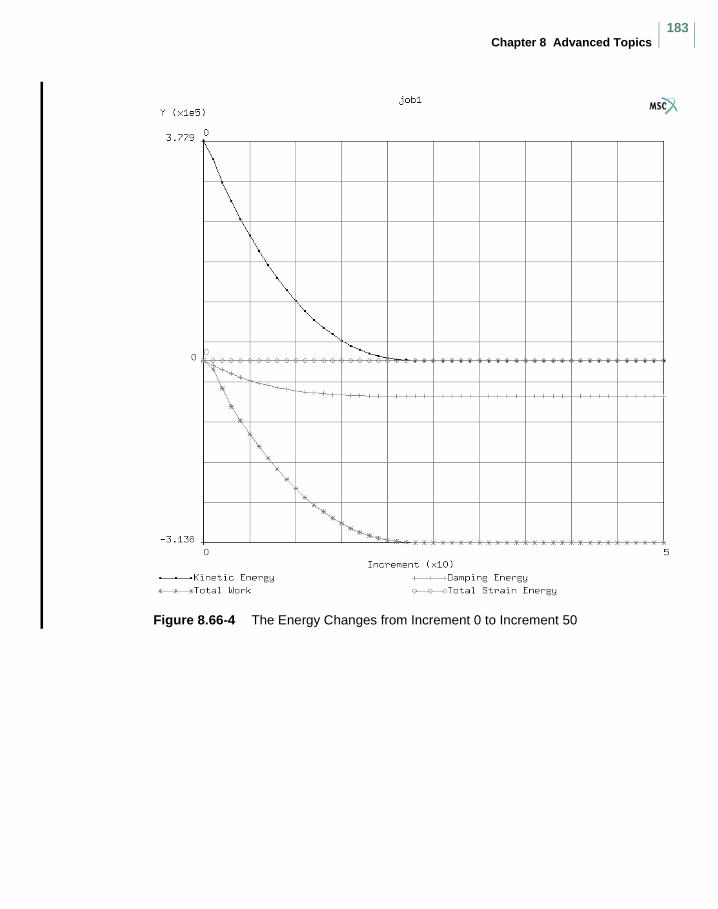
Chapter 8 Advanced Topics183
Figure 8.66-4 The Energy Changes from Increment 0 to Increment 50
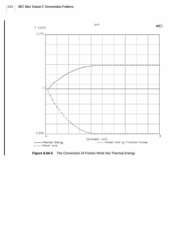
MSC.Marc Volume E: Demostration Problems
184
Figure 8.66-5 The Conversion of Friction Work into Thermal Energy

Chapter 8 Advanced Topics185
8.67 Analysis of an Automobile Tire3-D finite element analysis of automobile tires is complicated because of the complex structure of tires which are made of several types of rubber, reinforced with cord layers and a steal core. This problem demonstrates the use of Marc’s axisymmetric to 3-D data transfer capability for rebar elements. An automobile tire with a smooth tread, denoted as 195/65/R15, is analyzed. See [Helnwein et al., “A new 3D finite element model for cord-reinforced rubber composites - Application to analysis of automobile tires”, Finite Elements in Analysis and Design, Vol. 14, 1-16(1993)] for detailed description of the model. The analysis includes the numerical simulation of three steps: (1) mounting the tire on the wheel, (2) inflating the tire up to 2.0 bar, and (3) pressing it against a road surface.
During the first two steps, the deformation is purely axisymmetric and, therefore, an axisymmetric analysis is performed. See e8x67a.dat. The simulation of tire mounting on the wheel is carried out using 10 equal increments. Afterwards, the inflation pressure is applied with 10 more equal increments. In the third step, the tire contacts with the road surface. The problem becomes fully three dimensional. See e8x67b.dat. A total vertical movement of 25 mm of the tire against the road surface is applied using the AUTO STEP option and the analysis is completed after 13 increments. In e8x67b.dat, the AXITO3D option is used to transfer data from axisymmetric mesh (e8x67a.dat) to 3-D mesh (e8x67b.dat).
Model
In axisymmetric analysis (e8x67a.dat), the tire is modeled with 180 4-node isoparametric quadrilateral axisymmetric elements. Among them, 120 elements (element type 10) are used to model the rubber materials and 60 rebar elements (element type 144) are used to model the reinforcing cords. The axisymmetric mesh is shown in Figure 8.67-1. There are 162 nodes in the mesh. The tire wheel is modeled using an analytical rigid curve.
The 3-D model (see Figure 8.67-2), containing 3120 rubber elements (element type 7) and 1560 rebar elements (element type 146), is obtained by expanding the axisymmetric model in Figure 8.67-1, using EXPAND =>AXISYMMETRIC MODEL TO 3D option in Mentat. There are totally 4680 8-node isoparametric hexahedral elements and 4212 nodes in the 3-D model. The curve representing rigid wheel is also expanded automatically with the mesh into a 3-D rigid surface. The road is modeled as a flat rigid surface.
MSC.Marc Volume E: Demostration Problems
186
Elements
The element types 10 and 144 are used in the axisymmetric run. The corresponding 3-D element types are 7 and 146. ELASTICITY,2 activates the updated Lagrangian formulation. However, internally rebar elements always use total Lagrangian framework.
Material Properties
The rubber is modeled using Mooney constitutive model. The material properties are:
Tread: C1 = 0.35 N/mm2 and C2 = 0.16 N/mm2;
Base: C1 = 0.58 N/mm2 and C2 = 0.26 N/mm2;
Other part: C1 = 0.45 N/mm2 and C2 = 0.36 N/mm2.
The bead core and reinforcing cords are modeled with isotropic materials. The material properties are:
Bead core and steel belts:Young’s modulus 198700 N/mm2 and Poisson’s ratio 0.3;
Carcasses: Young’s modulus 6800 N/mm2 and Poisson’s ratio 0.3;
Cap ply: Young’s modulus 1950 N/mm2 and Poisson’s ratio 0.3.
Rebar layer properties are defined using REBAR option. See e8x67a.dat and e8x67b.dat for details.
Boundary Conditions and Load Definitions
In axisymmetric analysis (e8x67a.dat), there are three sets of boundary and load definitions. The mounting of the tire into the wheel is simulated using a set of point loads. The set of loads is then released after the mounting is completed. A set of symmetric condition is applied to remove the rigid body motion. The inflation pressure is applied to the inner surface of the tire within 10 equal increments.
In 3-D analysis (e8x67b.dat), the symmetric condition and the point loads are no longer needed and inflation pressure is unchanged. To simulate the tire-road contact, the flat, rigid surface moves up 25 mm against the tire. The AUTO STEP option is used.
Chapter 8 Advanced Topics187
Results
The deformed and the undeformed mesh after the tire inflation is in Figure 8.67-3. The final deformed shape of the 3-D tire model is shown in Figure 8.67-4. The contact pressure after 25 mm contact displacements is shown in Figure 8.67-5.
Parameters, Options, and Subroutines Summary
e8x67a.dat
e8x67b.dat
Parameters Model Definition Options History Definition Options
ALL POINTS CONNECTIVITY AUTO LOADDIST LOADS CONTACT CONTINUEELASTICITY COORDINATES CONTROLELEMENTS DEFINE DIST LOADSEND DIST LOADS MOTION CHANGEPROCESSOR END OPTION POINT LOADSETNAME FIXED DISP TIME STEPSIZING ISOTROPIC TITLETITLE MOONEY
NO PRINTOPTIMIZEPOINT LOADPOSTREBARSOLVER
Parameters Model Definition Options History Definition Options
ALL POINTS AXITO3D AUTO STEPDIST LOADS CONNECTIVITY CONTINUEELASTICITY CONTACT CONTROLELEMENTS COORDINATES DIST LOADSEND DEFINE MOTION CHANGEPROCESSOR DIST LOADS TITLESETNAME END OPTIONSIZING ISOTROPICTITLE MOONEY
NO PRINTOPTIMIZEPOSTREBARSOLVER
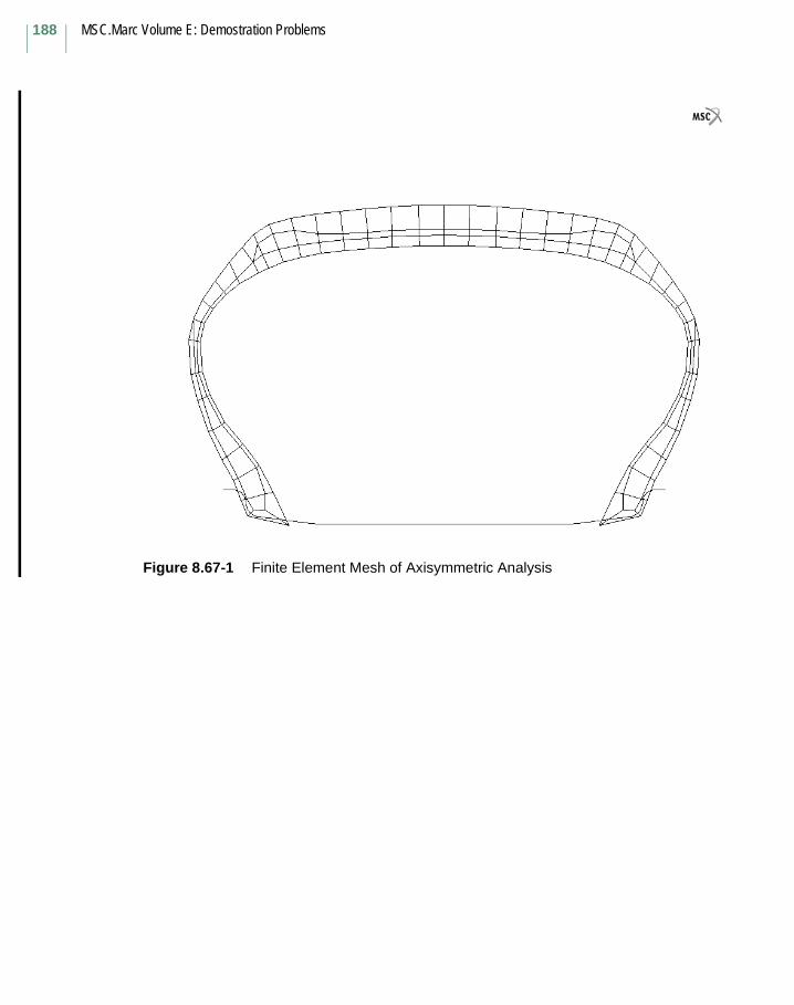
MSC.Marc Volume E: Demostration Problems
188
Figure 8.67-1 Finite Element Mesh of Axisymmetric Analysis
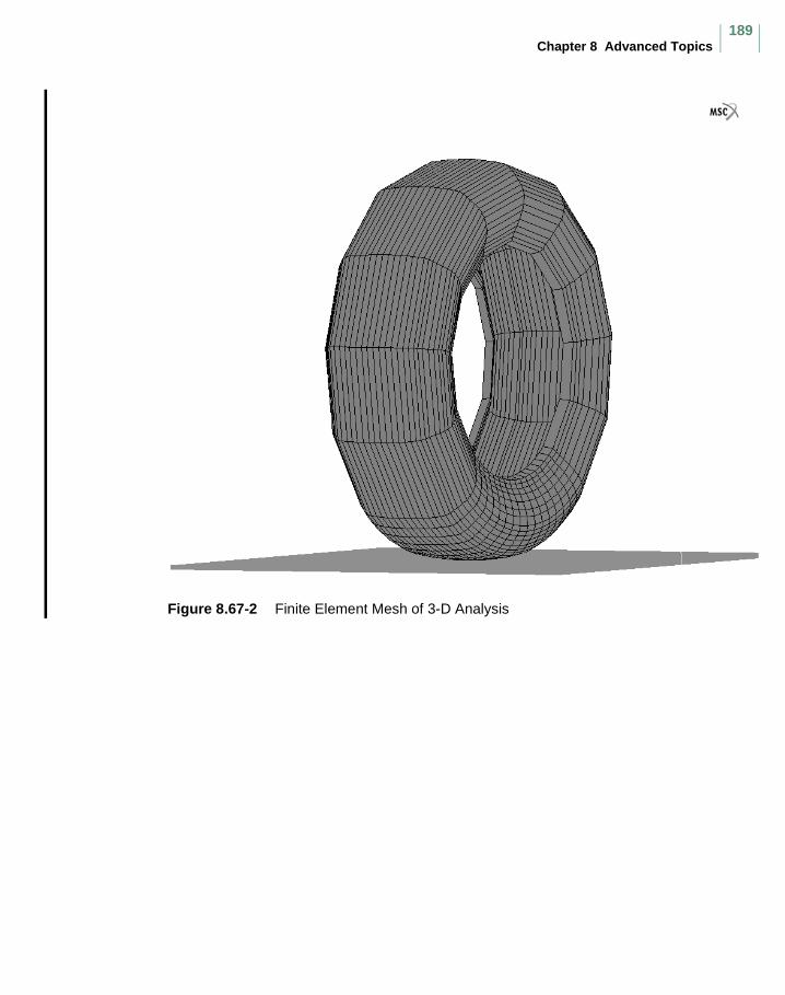
Chapter 8 Advanced Topics189
Figure 8.67-2 Finite Element Mesh of 3-D Analysis
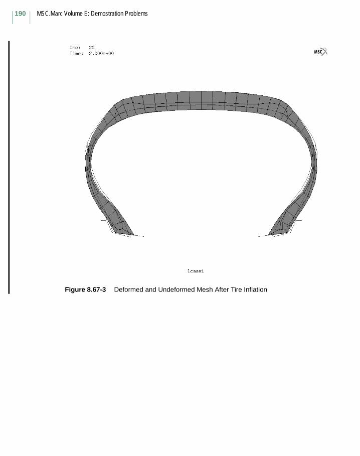
MSC.Marc Volume E: Demostration Problems
190
Figure 8.67-3 Deformed and Undeformed Mesh After Tire Inflation
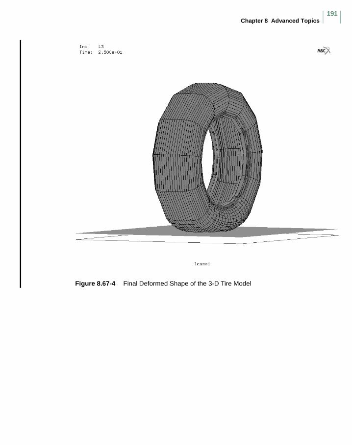
Chapter 8 Advanced Topics191
Figure 8.67-4 Final Deformed Shape of the 3-D Tire Model
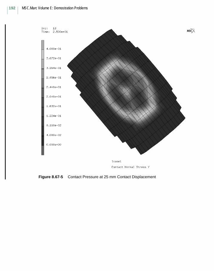
MSC.Marc Volume E: Demostration Problems
192
Figure 8.67-5 Contact Pressure at 25 mm Contact Displacement
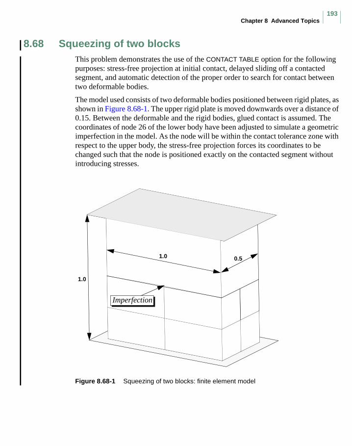
Chapter 8 Advanced Topics193
8.68 Squeezing of two blocksThis problem demonstrates the use of the CONTACT TABLE option for the following purposes: stress-free projection at initial contact, delayed sliding off a contacted segment, and automatic detection of the proper order to search for contact between two deformable bodies.
The model used consists of two deformable bodies positioned between rigid plates, as shown in Figure 8.68-1. The upper rigid plate is moved downwards over a distance of 0.15. Between the deformable and the rigid bodies, glued contact is assumed. The coordinates of node 26 of the lower body have been adjusted to simulate a geometric imperfection in the model. As the node will be within the contact tolerance zone with respect to the upper body, the stress-free projection forces its coordinates to be changed such that the node is positioned exactly on the contacted segment without introducing stresses.
Figure 8.68-1 Squeezing of two blocks: finite element model
1.0
1.0
0.5
Imperfection
MSC.Marc Volume E: Demostration Problems
194
During the analysis, adaptive mesh refinement is applied. As a result, in increment 1, the mesh density of the upper body is equal to that of the lower body and from increment 2 onwards, the mesh density of the upper body is larger than that of the lower body. This is accounted for by automatically adapting the search order for contact.
The different material properties of the deformable bodies cause a difference between the lateral displacements of the nodes in the contact area between the deformable bodies. The delayed sliding off option forces nodes not to slide off a contacted segment at a sharp corner, but to remain in contact until it has moved over 10 times the contact tolerance beyond the edge of the contacted segment.
Elements
Element 7, an eight-node brick element with full integration, is used in this example. The initial finite element mesh contains nine elements.
Large disp
The LARGE DISP parameter option is used to perform a geometrically nonlinear analysis.
Adaptive
Due to adaptive mesh refinement there will be increase in the number of nodes and elements. With the ADAPTIVE parameter option the upper bound to the number of nodes and elements is set to 500.
Isotropic
The material properties are given by Young’s modulus and Poisson’s
ratio for the lower body and and for the upper body.
These properties are entered via the ISOTROPIC model definition option.
Contact
Two deformable and two rigid bodies are defined. The lower deformable body consists of eight elements and the upper deformable body of one element. Each of the two rigid bodies consists of a flat surface.
E 14×10=
ν 0.3= E 93×10= ν 0.34=
Chapter 8 Advanced Topics195
Contact Table
The CONTACT TABLE model definition option is used to activate the following:
• Glued contact between the rigid and deformable bodies;
• Automatic determination of the optimal order to search for contact, based on the element edge length at the boundary of the contact bodies (a check on contact will be performed only for nodes corresponding to the body with the smallest element edge length);
• Stress-free projection at initial contact;
• Delayed sliding off a contacted segment at a sharp corner.
Adaptive
The “node in contact” criterion for adaptive mesh refinement is activated for element 1. The maximum number of refinement levels is set to 2.
No print
The NO PRINT model definition option is used to suppress print out.
Post
The default nodal variables are put on the post file. The stress tensor is selected as an element variable.
Control
The default control settings are used: convergence checking is done based on residual forces with a tolerance of 0.1.
Motion Change
The velocity of the upper rigid body in y-direction is set to -0.15.
Results
Figure 8.68-2 shows the model in increment 0. Clearly, due to the stress-free projection, the geometric imperfection has been removed by adjusting the coordinates of node 26. The contour band plot of the contact status shows that nodes of the lower deformable body are touching the upper deformable body. In Figure 8.68-3, the mesh density of the upper body has changed due to adaptive remeshing and nodes of the upper deformable body are now touching the lower deformable body. Finally,
MSC.Marc Volume E: Demostration Problems
196
Figure 8.68-4 shows the effect of the delayed sliding off option: nodes at the outer edge of the upper deformable body passed the edge of the contacted segment of the lower body, but still remain in contact.
Parameters, Options, and Subroutines Summary
Example e8x68.dat:
Parameters Model Definition Options History Definition Options
ADAPTIVE CONNECTIVITY AUTO LOAD
ELEMENTS CONTACT CONTINUE
END CONTACT TABLE CONTROL
EXTENDED COORDINATES MOTION CHANGE
LARGE DISP DEFINE TIME STEP
SETNAME END OPTION
SIZING ISOTROPIC
TITLE NO PRINT
OPTIMIZE
POST
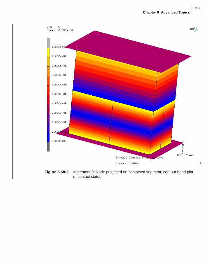
Chapter 8 Advanced Topics197
Figure 8.68-2 Increment 0: Node projected on contacted segment; contour band plot of contact status
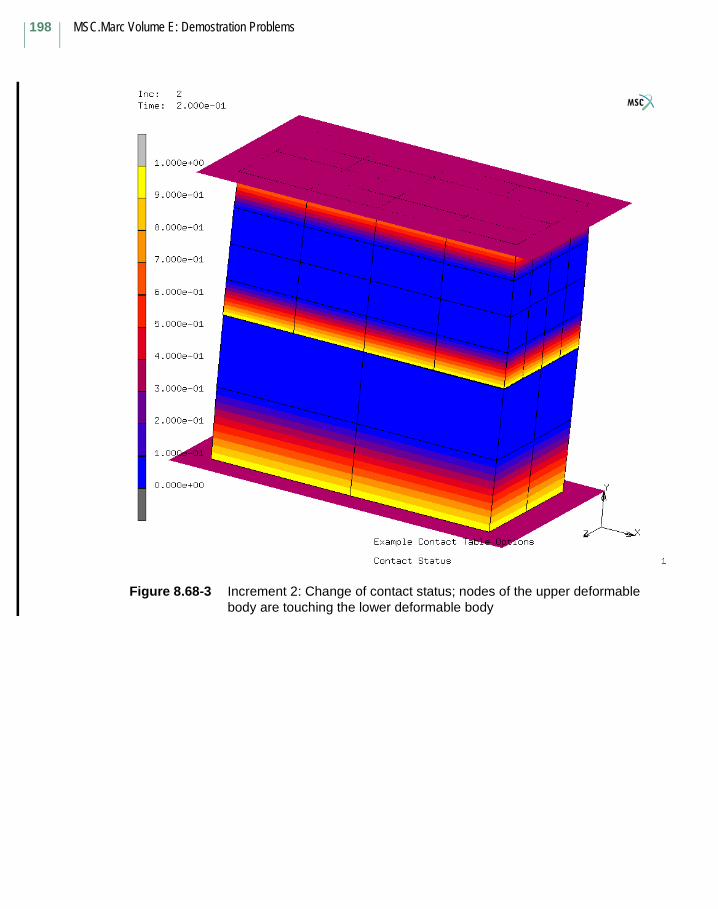
MSC.Marc Volume E: Demostration Problems
198
Figure 8.68-3 Increment 2: Change of contact status; nodes of the upper deformable body are touching the lower deformable body
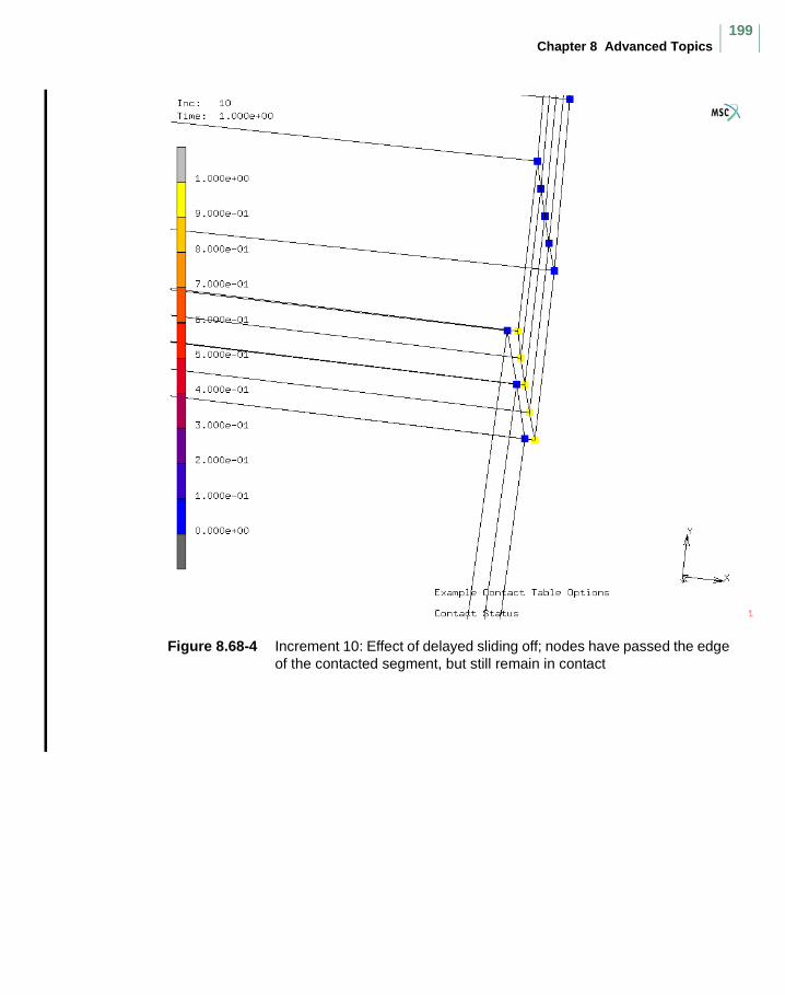
Chapter 8 Advanced Topics199
Figure 8.68-4 Increment 10: Effect of delayed sliding off; nodes have passed the edge of the contacted segment, but still remain in contact

MSC.Marc Volume E: Demostration Problems
200


