MS&E 211Quadratic Programming

Ashish Goel

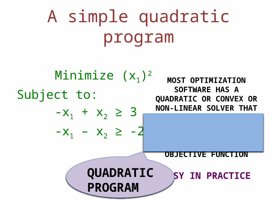
A simple quadratic program

Minimize (x1)2

Subject to:-x1 + x2 ≥ 3

-x1 – x2 ≥ -2

A simple quadratic program

Minimize (x1)2

Subject to:-x1 + x2 ≥ 3

-x1 – x2 ≥ -2

MOST OPTIMIZATION SOFTWARE HAS A QUADRATIC OR CONVEX OR NON-LINEAR SOLVER THAT

CAN BE USED TO SOLVE MATHEMATICAL PROGRAMS

WITH LINEAR CONSTRAINTS AND A MIN-QUADRATIC OBJECTIVE

FUNCTION

EASY IN PRACTICE

A simple quadratic program

Minimize (x1)2

Subject to:-x1 + x2 ≥ 3

-x1 – x2 ≥ -2

MOST OPTIMIZATION SOFTWARE HAS A QUADRATIC OR CONVEX OR NON-LINEAR SOLVER THAT

CAN BE USED TO SOLVE MATHEMATICAL PROGRAMS

WITH LINEAR CONSTRAINTS AND A MIN-QUADRATIC OBJECTIVE

FUNCTION

EASY IN PRACTICEQUADRATICPROGRAM

Next Steps

• Why are Quadratic programs (QPs) easy?

• Formal Definition of QPs

• Examples of QPs

Next Steps

• Why are Quadratic programs (QPs) easy?– Intuition; not formal proof

• Formal Definition of QPs

• Examples of QPs– Regression and Portfolio Optimization

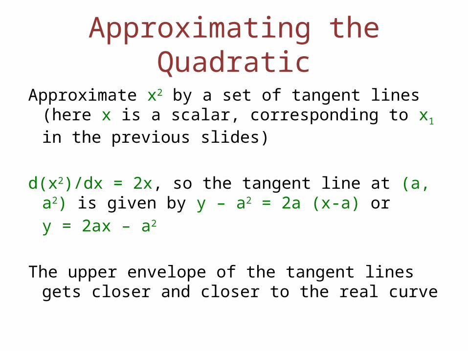
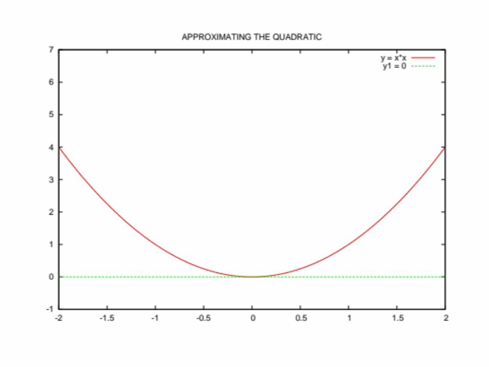
Approximating the Quadratic

Approximate x2 by a set of tangent lines (here x is a scalar, corresponding to x1 in the previous slides)

d(x2)/dx = 2x, so the tangent line at (a, a2) is given by y – a2 = 2a (x-a) or

y = 2ax – a2

The upper envelope of the tangent lines gets closer and closer to the real curve

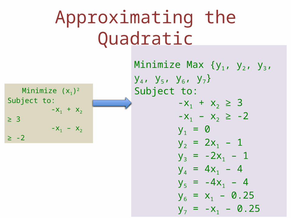
Approximating the Quadratic

Minimize Max {y1, y2, y3, y4, y5, y6, y7}Subject to:

-x1 + x2 ≥ 3-x1 – x2 ≥ -2y1 = 0y2 = 2x1 – 1y3 = -2x1 – 1y4 = 4x1 – 4y5 = -4x1 – 4y6 = x1 – 0.25y7 = -x1 – 0.25

Minimize (x1)2

Subject to:

-x1 + x2 ≥ 3

-x1 – x2 ≥ -2

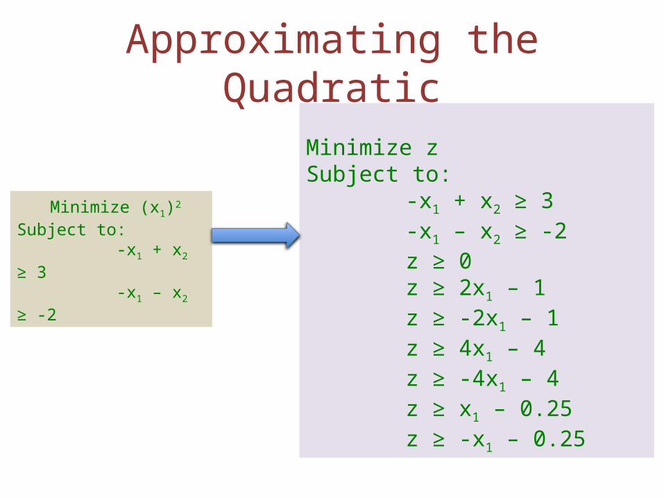
Approximating the Quadratic

Minimize zSubject to:

-x1 + x2 ≥ 3-x1 – x2 ≥ -2z ≥ 0z ≥ 2x1 – 1z ≥ -2x1 – 1z ≥ 4x1 – 4z ≥ -4x1 – 4z ≥ x1 – 0.25z ≥ -x1 – 0.25

Minimize (x1)2

Subject to:

-x1 + x2 ≥ 3

-x1 – x2 ≥ -2

Approximating the Quadratic

Minimize zSubject to:

-x1 + x2 ≥ 3-x1 – x2 ≥ -2z ≥ 0z ≥ 2x1 – 1z ≥ -2x1 – 1z ≥ 4x1 – 4z ≥ -4x1 – 4z ≥ x1 – 0.25z ≥ -x1 – 0.25

Minimize (x1)2

Subject to:

-x1 + x2 ≥ 3

-x1 – x2 ≥ -2

LPs can give successively better approximations

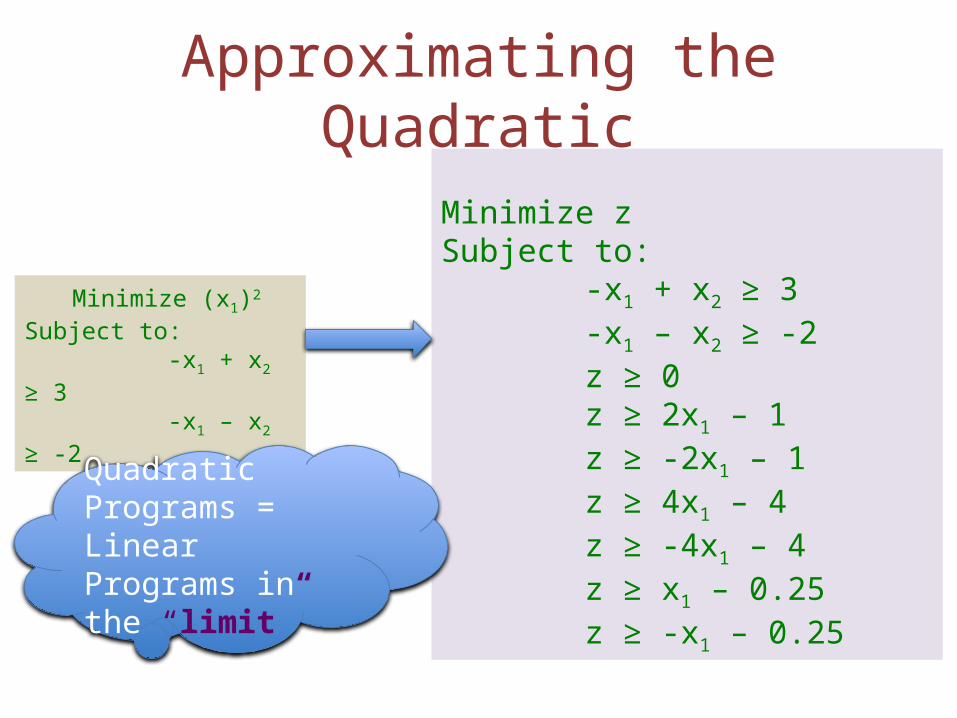
Approximating the Quadratic

Minimize zSubject to:

-x1 + x2 ≥ 3-x1 – x2 ≥ -2z ≥ 0z ≥ 2x1 – 1z ≥ -2x1 – 1z ≥ 4x1 – 4z ≥ -4x1 – 4z ≥ x1 – 0.25z ≥ -x1 – 0.25

Minimize (x1)2

Subject to:

-x1 + x2 ≥ 3

-x1 – x2 ≥ -2

Quadratic Programs = Linear Programs in the “limit”

QPs and LPs

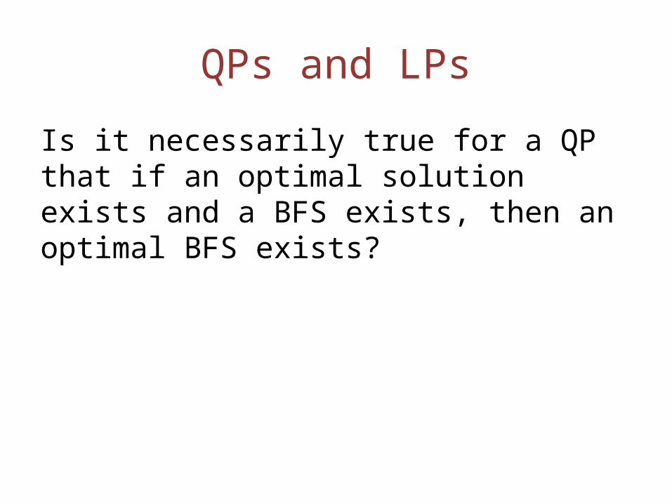
Is it necessarily true for a QP that if an optimal solution exists and a BFS exists, then an optimal BFS exists?

QPs and LPs

Is it necessarily true for a QP that if an optimal solution exists and a BFS exists, then an optimal BFS exists?

NO!!

Intuition: When we think of a QP as being approximated by a succession of LPs, we have to add many new variables and constraints; the BFS of the new LP may not be the same as the BFS of the feasible region for the original constraints.

QPs and LPs

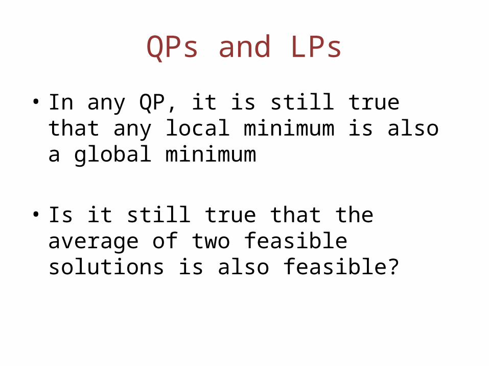
• In any QP, it is still true that any local minimum is also a global minimum

• Is it still true that the average of two feasible solutions is also feasible?

QPs and LPs

• In any QP, it is still true that any local minimum is also a global minimum

• Is it still true that the average of two feasible solutions is also feasible?– Yes!!

QPs and LPs

• In any QP, it is still true that any local minimum is also a global minimum

• Is it still true that the average of two feasible solutions is also feasible?– Yes!!

• QPs still have enough nice structure that they are easy to solve

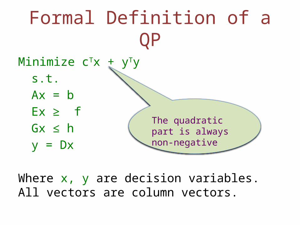
Formal Definition of a QP

Minimize cTx + yTys.t.

Ax = bEx ≥ fGx ≤ hy = Dx

Where x, y are decision variables. All vectors are column vectors.

Formal Definition of a QP

Minimize cTx + yTys.t.

Ax = bEx ≥ fGx ≤ hy = Dx

Where x, y are decision variables. All vectors are column vectors.

The quadratic part is always non-negative

Minimize cTx + yTys.t.

Ax = bEx ≥ fGx ≤ hy = Dx

Where x, y are decision variables. All vectors are column vectors.

Formal Definition of a QP

i.e. ANY LINEAR CONSTRAINTS

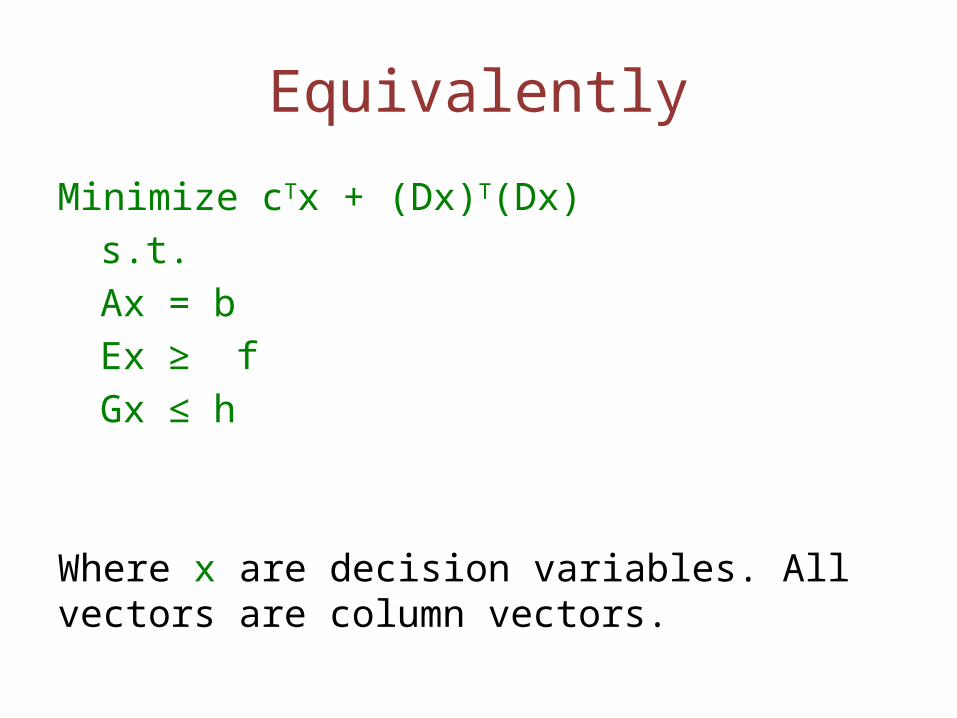
Equivalently

Minimize cTx + (Dx)T(Dx)s.t.

Ax = bEx ≥ fGx ≤ h

Where x are decision variables. All vectors are column vectors.

Equivalently

Minimize cTx + xTDTDxs.t.

Ax = bEx ≥ fGx ≤ h

Where x are decision variables. All vectors are column vectors.

Equivalently

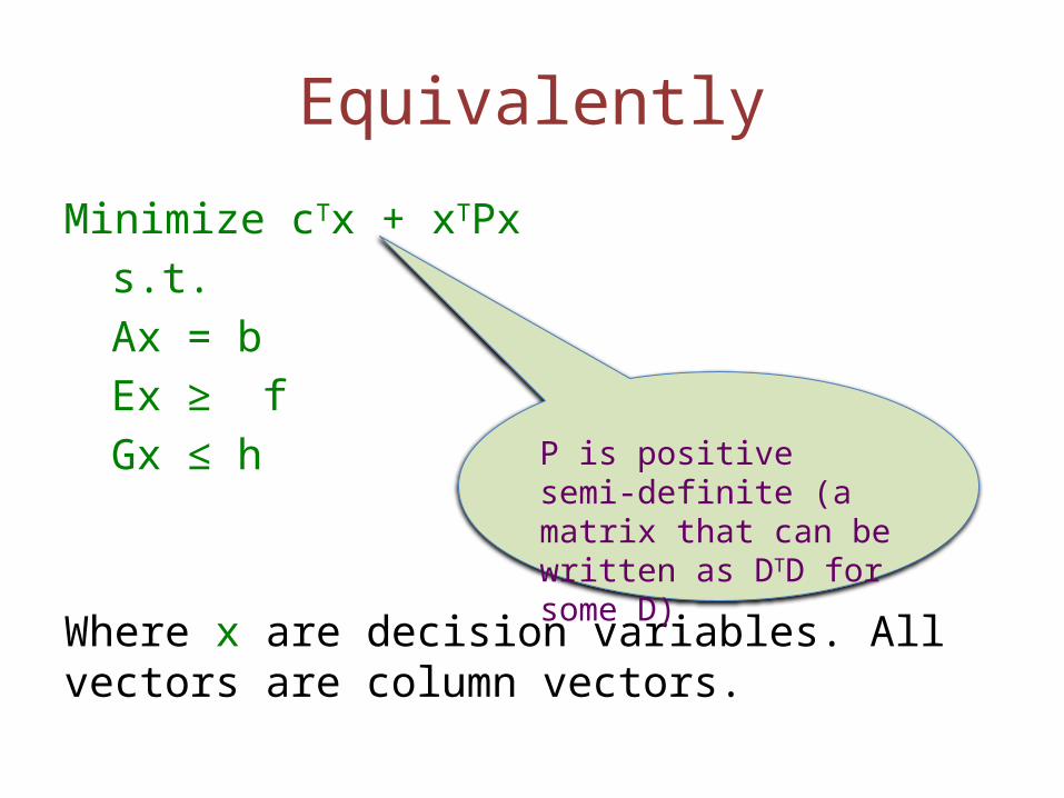
Minimize cTx + xTPxs.t.

Ax = bEx ≥ fGx ≤ h

Where x are decision variables. All vectors are column vectors.

P is positive semi-definite (a matrix that can be written as DTD for some D)

Equivalently

Minimize cTx + yTys.t.

Ax = bEx ≥ fGx ≤ h

Where x are decision variables, and y represents a subset of the coordinates of x. All vectors are column vectors.

Equivalently

Instead of minimizing, the objective function is

Maximize cTx – xTPx

For some positive semi-definite matrix P

Is this a QP?

Minimize xys.t.

x + y = 5

Is this a QP?

Minimize xys.t.

x + y = 5

No, since x = 1, y=-1 gives xy = -1. Hence xy is not an acceptable quadratic part for the objective function.

Is this a QP?

Minimize xys.t.

x + y = 5x, y ≥ 0

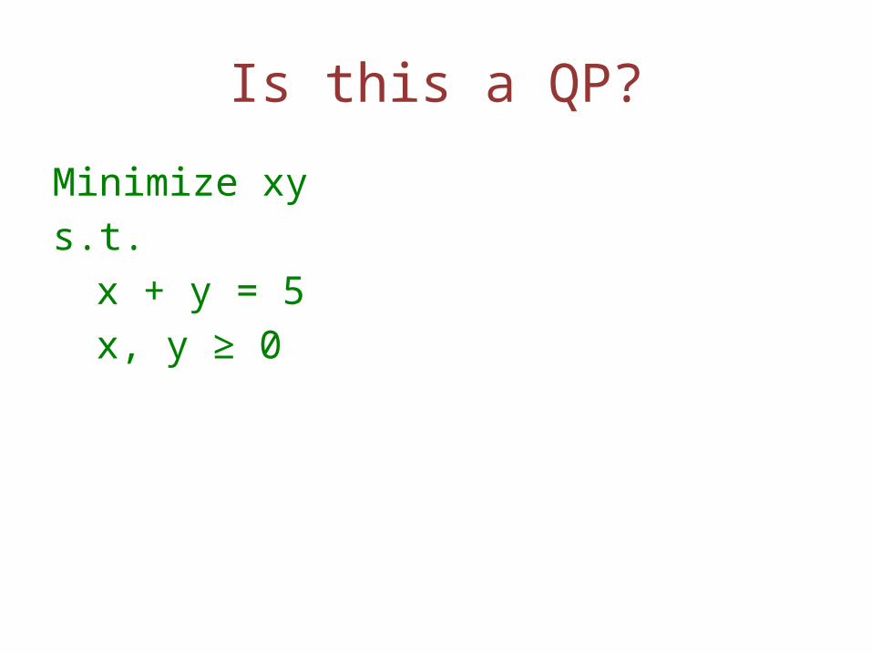
Is this a QP?

Minimize xys.t.

x + y = 5x, y ≥ 0

No, for the same reason as before!

Is this a QP?

Minimize x2 -2xy + y2 - 2x

s.t.x + y = 5

Is this a QP?

Minimize x2 -2xy + y2 - 2x

s.t.x + y = 5

Yes, since we can write the quadratic part as (x-y)(x-y).

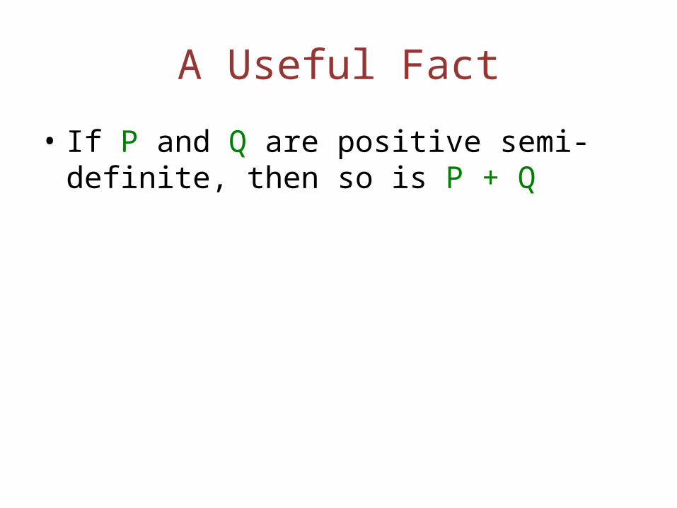
A Useful Fact

• If P and Q are positive semi-definite, then so is P + Q

An example: Linear Regression

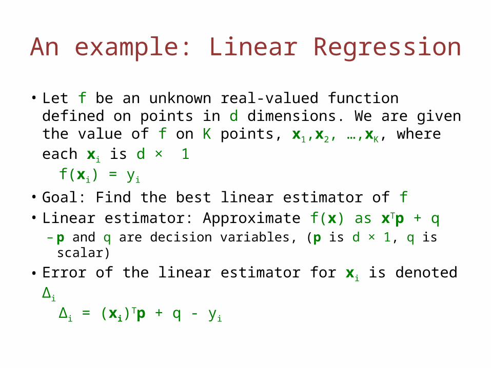
• Let f be an unknown real-valued function defined on points in d dimensions. We are given the value of f on K points, x1,x2, …,xK, where each xi is d × 1

f(xi) = yi

• Goal: Find the best linear estimator of f• Linear estimator: Approximate f(x) as xTp + q– p and q are decision variables, (p is d × 1, q is scalar)

• Error of the linear estimator for xi is denoted Δi

Δi = (xi)Tp + q - yi

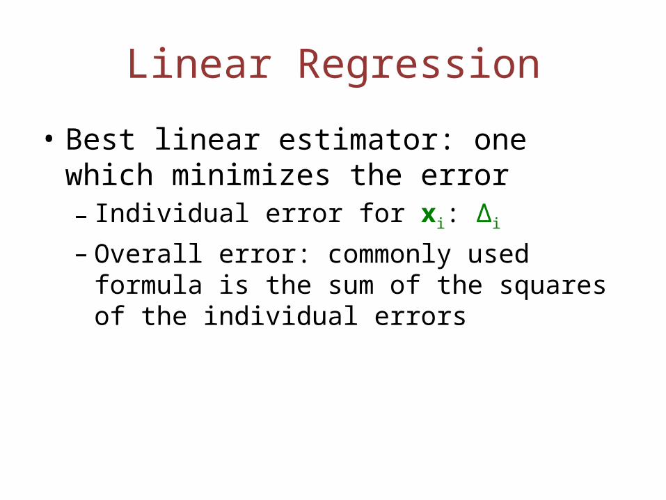
Linear Regression

• Best linear estimator: one which minimizes the error– Individual error for xi: Δi

– Overall error: commonly used formula is the sum of the squares of the individual errors

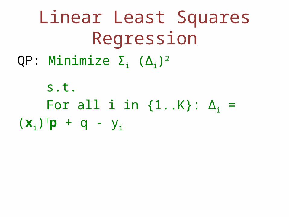
Linear Least Squares Regression

QP: Minimize Σi (Δi)2

s.t.For all i in {1..K}: Δi = (xi)Tp + q - yi

Linear Least Squares Regression

QP: Minimize Σi (Δi)2

s.t.For all i in {1..K}: Δi = (xi)Tp + q - yi

Can simplify this further.

Linear Least Squares Regression

QP: Minimize Σi (Δi)2

s.t.For all i in {1..K}: Δi = (xi)Tp + q - yi

Can simplify this further. Let X denote the d × K matrix obtained from all the xi ’s: X = (x1 x2

… xK)

Linear Least Squares Regression

QP: Minimize Σi (Δi)2

s.t.For all i in {1..K}: Δi = (xi)Tp + q - yi

Can simplify this further. Let X denote the d × K matrix obtained from all the xi ’s: X = (x1 x2

… xK)

Let e denote a K × 1 vector of all 1’s

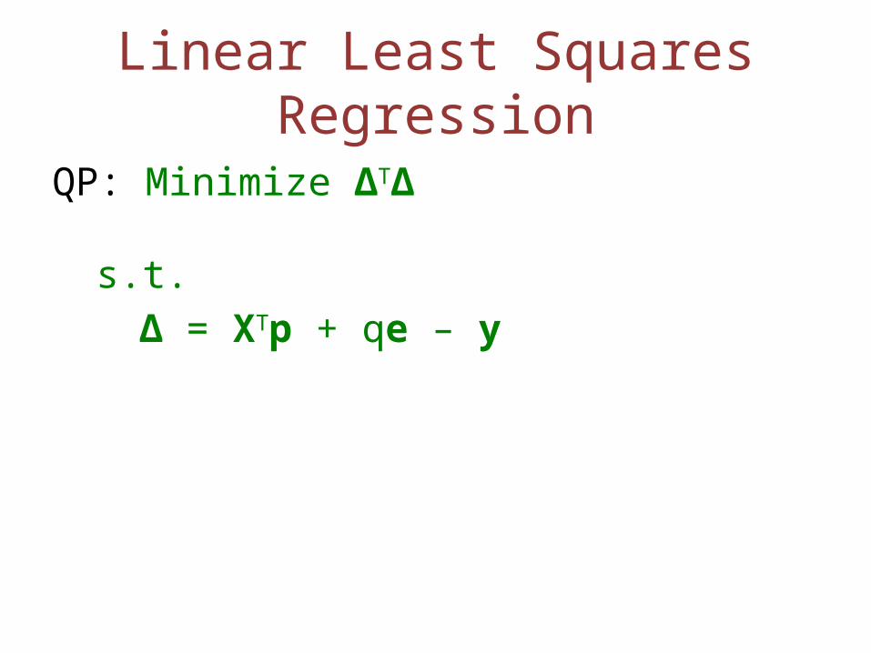
Linear Least Squares Regression

QP: Minimize ΔTΔ

s.t.Δ = XTp + qe – y

Simple Portfolio Optimization

• Consider a market with N financial products (stocks, bonds, currencies, etc.) and M future market scenarios

• Payoff matrix P: Pi,j = Payoff from product j in the i-th scenario

• xj = # of units bought of j-th product

• cj = cost per unit of j-th product

• Additional assumption: Probability qi of market scenario i happening is given

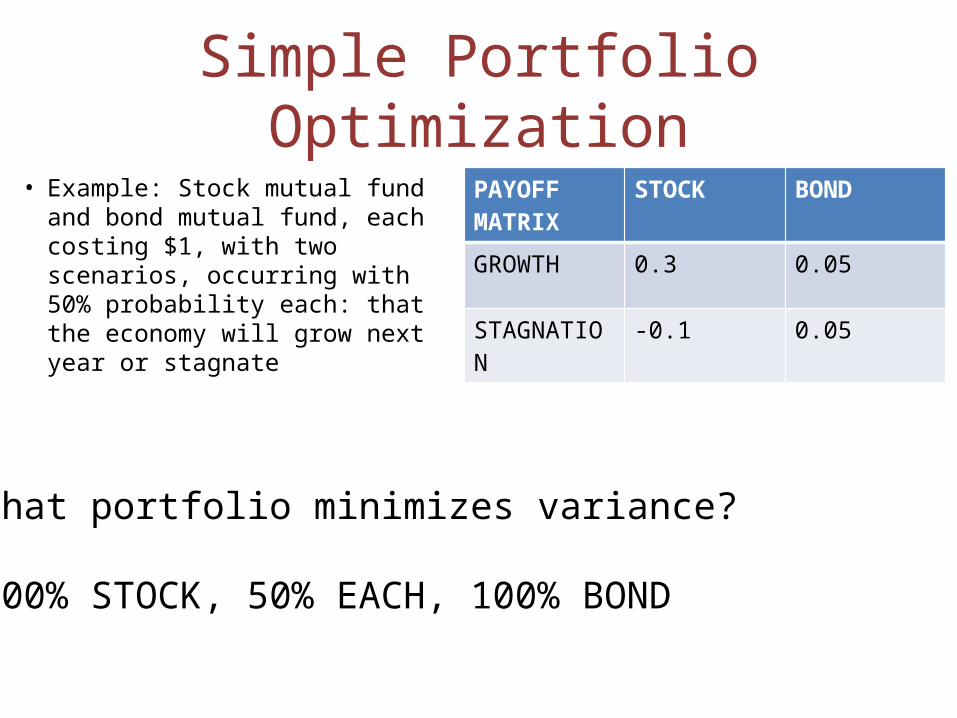
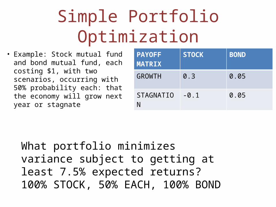
Simple Portfolio Optimization• Example: Stock mutual fund

and bond mutual fund, each costing $1, with two scenarios, occurring with 50% probability each: that the economy will grow next year or stagnate

PAYOFF MATRIX

STOCK BOND

GROWTH 0.3 0.05

STAGNATION -0.1 0.05

Simple Portfolio Optimization• Example: Stock mutual fund

and bond mutual fund, each costing $1, with two scenarios, occurring with 50% probability each: that the economy will grow next year or stagnate

PAYOFF MATRIX

STOCK BOND

GROWTH 0.3 0.05

STAGNATION -0.1 0.05

What portfolio maximizes expected payoff?

100% STOCK, 50% EACH, 100% BOND

Simple Portfolio Optimization• Example: Stock mutual fund

and bond mutual fund, each costing $1, with two scenarios, occurring with 50% probability each: that the economy will grow next year or stagnate

PAYOFF MATRIX

STOCK BOND

GROWTH 0.3 0.05

STAGNATION -0.1 0.05

What portfolio maximizes expected payoff?

100% STOCK, 50% EACH, 100% BOND

Simple Portfolio Optimization• Example: Stock mutual fund

and bond mutual fund, each costing $1, with two scenarios, occurring with 50% probability each: that the economy will grow next year or stagnate

PAYOFF MATRIX

STOCK BOND

GROWTH 0.3 0.05

STAGNATION -0.1 0.05

What portfolio minimizes variance?

100% STOCK, 50% EACH, 100% BOND

Simple Portfolio Optimization• Example: Stock mutual fund

and bond mutual fund, each costing $1, with two scenarios, occurring with 50% probability each: that the economy will grow next year or stagnate

PAYOFF MATRIX

STOCK BOND

GROWTH 0.3 0.05

STAGNATION -0.1 0.05

What portfolio minimizes variance?

100% STOCK, 50% EACH, 100% BOND

Simple Portfolio Optimization• Example: Stock mutual fund

and bond mutual fund, each costing $1, with two scenarios, occurring with 50% probability each: that the economy will grow next year or stagnate

PAYOFF MATRIX

STOCK BOND

GROWTH 0.3 0.05

STAGNATION -0.1 0.05

What portfolio minimizes variance subject to getting at least 7.5% expected returns?100% STOCK, 50% EACH, 100% BOND

Simple Portfolio Optimization• Example: Stock mutual fund

and bond mutual fund, each costing $1, with two scenarios, occurring with 50% probability each: that the economy will grow next year or stagnate

PAYOFF MATRIX

STOCK BOND

GROWTH 0.3 0.05

STAGNATION -0.1 0.05

What portfolio minimizes variance subject to getting at least 7.5% expected returns?100% STOCK, 50% EACH, 100% BOND

Minimizing Variance (≈ Risk)

• Often, we want to minimize the variance of our portfolio, subject to some cost budget b and some payoff target π

• Let yi denote the payoff in market scenario iyi = Pix

• Expected payoff= z = Σi qiyi = qTy

• Variance = Σi qi(yi - z)2 = Σi ((qi)1/2(yi - z))2

• Let vi denote (qi)1/2(yi – z)

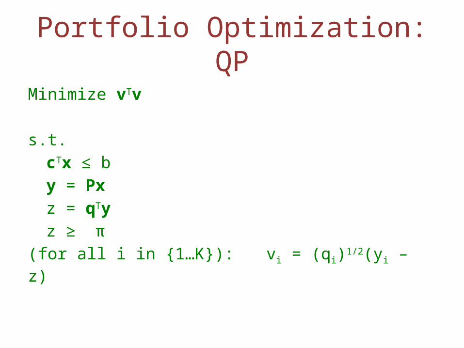
Portfolio Optimization: QP

Minimize vTv

s.t.cTx ≤ by = Pxz = qTyz ≥ π

(for all i in {1…K}): vi = (qi)1/2(yi – z)

THANK YOU!!!