MSX.60 series resistancepdf.pdf

(IJACSA) International Journal of Advanced Computer Science and Applications, Vol. 5, No. 1, 2014

129 | P a g e www.ijacsa.thesai.org

Modelling and Output Power Evaluation of Series-

Parallel Photovoltaic Modules

Dr. Fadi N. Sibai

Process & Control Systems Department

Saudi Aramco

Dhahran 31311, Kingdom of Saudi Arabia

Abstract—Solar energy has received attention in the Middle

East given the abundant and free irradiance and extended sunny

weather. Although photovoltaic panels were introduced decades

ago, they have recently become economical and gained traction.

We present a mathematical model for series-parallel photovoltaic

modules, evaluate the model, and present the I-V and P-V

characteristic plots for various temperatures, irradiance, and

diode ideality factors. The power performance results are then

analyzed and recommendations are made. Unlike other related

work, our evaluation uses standard spreadsheet software

avoiding commercial simulation packages and application

programming. Results indicate improved power performance

with irradiance and parallel connections of cell series branches.

Given the hot weather in our region, increasing the number of cells connected in series from 36 to 72 is not recommended.

Keywords—solar energy; series-parallel photovoltaic modules;

mathematical modeling

I. INTRODUCTION

The push for renewable energy solutions is steady to reduce carbon emissions, protect the environment and population health, and effect climate and sea water level changes. Solar energy has received attention in the Middle East given the abundant and free irradiance and sunny weather. Although photovoltaic (PV) panels were introduced decades ago, they have recently become economical and gained traction. Saudi Arabia recently saw the successful installation of a 3.5 megawatt photovoltaic field, the largest solar power plant built in the country, and has plans to install 41 Gigawatts of solar power over the next 20 years. PV fields geographically distributed can be located near loads and cut down on fuel consumed by power generating plants.

PV cells generate DC electricity during the day, which can be immediately consumed or stored in batteries for future consumption. An inverter is used to convert the generated power from DC to AC. The PV panel has a number of solar cells connected in series (typically 36 or 72) with the possibility to connect PV cell series branches in parallel. The solar cell is a p-n junction fabricated in a silicon (or other material) wafer or semiconductor layer. The photovoltaic effect causes the electromagnetic radiation of the solar energy hitting the PV cells to generate electricity. Photons with energy greater than the band gap energy of the wafer’s semiconductor material are absorbed, creating electron-hole pairs, which in turn create a photocurrent in the presence of the p-n junction’s internal electric field. The photocurrent’s magnitude rises with the

number of electron-hole pairs created, which is dependent on the irradiance level. Therefore the magnitude of the current generated by the PV module is proportional to the amount of incident solar radiation. PV module models have evolved to include detailed parameters and even multiple piecewise linear regions or better accuracy. However, most have focused on modeling a number of PV cells in series and stopped short of modeling multiple parallel branches of serially connected PV cells.

In this paper, we present a mathematical model for series-parallel photovoltaic modules, evaluate the model, and present the I-V (module current vs. module voltage) and P-V (module power vs. voltage) characteristic plots for various temperatures, irradiance and diode ideality factors. The power performance results are then analyzed and recommendations are made. Unlike others’ work, we model series-parallel PV cells with multiple parallel branches each consisting of a number of PV cells in series, and evaluate the model with a basic spreadsheet application, avoiding application programming and commercial simulators. This is facilitated by the mathematical technique (i.e. Newton-Raphson) used in the model evaluation which makes the model evaluation possible with a spreadsheet application. Thus, a key advantage of our approach is that our model can be reused by a larger population of researchers with no access to commercial simulator packages.

PV modeling and simulations are reviewed in Section II. In Section III, we present our mathematical model for a series-parallel PV module. In Section IV, the nonlinear model is evaluated in Excel and the I-V and P-V characteristics are plotted. Moreover, the results are analyzed for a variety of temperatures, irradiances, diode ideality factors, numbers of PV cells in series, and numbers of PV series branches connected in parallel. The paper concludes in Section V.

II. PV MODELING AND SIMULATIONS

PV cells and modules have been modeled [1-12] mathematically and/or within commercial simulators. Diode-based circuits have typically represented the PV module. PV models differ in the number of diodes they contain (1 or more). Maximum power tracking methods [2-5] were introduced to determine the best operating parameters for the module and allowing the PV module to generate the maximum power. MATLAB and SIMULINK codes for PV module have been presented in [5-8, 10-11]. Complete system simulation models including MPPT controller, battery, charger, and DC/DC converter were presented in [7]. Our work differs from prior



work in that we model series-parallel PV modules and evaluate the model with a simple spreadsheet application.

Effects of climatic and environmental factors on solar PV performance in arid desert regions were discussed in [9]. Movable non-fixed panels — that can reposition their surfaces toward the sun’s incident rays and track the sun’s path in the sky and dust removing techniques — are key to optimizing the PV panel’s output. The highest solar energy production in the Arabian Gulf region was determined to occur between 11 a.m. and 2 p.m. Cooling techniques were recommended to boost the module’s efficiencies in light of high temperature effects. Among relative humidity, temperature and dust, the PV module performance was found to be most affected by dust depositions during long operation times. Smart grid features and renewable energy integration requirements were reviewed in [13] which also introduced a micro inverter and simulated it proving that it meets leakage current standards.

Researchers [10] used various methods for modeling PV panels. Azab [11] presented a piecewise linear model with three diodes that allows simulations of mismatched panels working under different conditions. This piecewise linear model substitutes the single diode by three parallel diodes in the PV model and defines regions where different diodes are turned on. This piecewise linear results in smoother I-V and P-V curves than with the one diode model. Dondi et al [12] presented a PV cell model for solar energy powered sensor networks, suitable over a wide range of irradiance intensity, cell temperature variation and incident angle. Our simple model does not use Azab’s more precise piecewise linear model which increases the number of diodes (complexity) in the model, as we are mainly interested in determining the PV module’s maximum power output, which our model accurately derives.

Herein, we modify and generalize the PV model in [6] to model series-parallel PV cell modules with multiple parallel branches of PV cells in series.

III. SERIES-PARALLEL PV MODULE MODEL

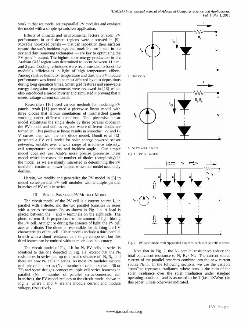
The circuit model of the PV cell is a current source IL in parallel with a diode, and the two parallel branches in series with a series resistance Rs, as shown in Fig. 1.a. A load is placed between the + and – terminals on the right side. The photo current IL is proportional to the amount of light hitting the PV cell. At night or during the absence of light, the PV cell acts as a diode. The diode is responsible for defining the I-V characteristics of the cell. Other models include a third parallel branch with a shunt resistance as a single component but this third branch can be omitted without much loss in accuracy.

The circuit model of Fig. 1.b for NS PV cells in series is identical to the one depicted in Fig. 1.a, except that the NS resistances in series add up to a total resistance of NS RS, and there are now NS cells in series. As most PV modules include multiple cells in series (NS = number of cells in series = 36 or 72) and some designs connect multiple cell series branches in parallel (NP = number of parallel series-connected cell branches), the PV model reduces to the circuit model shown in Fig. 2, where I and V are the module current and module voltage, respectively.

a. One PV cell

b. Ns PV cells in series

Fig. 1. PV cell models

Fig. 2. PV panel model with Np parallel branches, each with Ns cells in series

Note that in Fig. 2, the NP parallel resistances reduce the total equivalent resistance to NS RS / NP. The current source current of the parallel branches combine into the new current source NP IL. In the following sections, we use the variable “suns” to represent irradiance, where suns is the ratio of the solar irradiance over the solar irradiation under standard operating condition, and is assumed to be 1 (i.e., 1KW/m2) in this paper, unless otherwise indicated.



Nomenclature of the mathematical PV model follows.

IL: photo current

I0: saturation current

IS: photo current

Suns: irradiance = G/Gnom (where 1sun = 1KW/m2)

TaC: temperature in degrees Celsius

TaK: temperature in degrees Kelvin

Vg: band gap energy = 1.12V at temperature T1

T1: reference start temperature (in deg. K)

T2: reference end temperature (in deg. K)

T: junction temperature (in deg. K)

VOC_T1: open-circuit voltage at temperature T1

VOC_T2: open-circuit voltage at temperature T2

ISC_T1: short-circuit current at temperature T1

ISC_T2: short-circuit current at temperature T2

RS: series resistance

NS: number of series-connected cells

NP: number of parallel-connected cells

q: electron charge = 1.6E-19 Coul.

k: Boltzmann’s constant = 1.38E-23 J/K

G: irradiance

n: diode ideality factor between 1(ideal) and 2

The PV module current I pictured in Fig. 2 is the photo current IL minus the diode current and is given by

I= NP IL - NP I0 (eq (V / Ns + I Rs / Np) / (n k TaK) - 1) (1)

Note that I appears on both sides of the equation. As under constant radiance and temperature IL is constant, I is therefore a constant minus the exponential-shaped diode current, and takes the shape of the curve of Fig. 3.

Fig. 3. Typical I-V characteristic curve of a PV module

The point (Voptimal, Ioptimal) is of interest as it is the point at which the PV module’s output power is maximum and is therefore a desired operation point. The I-V curve crosses the horizontal V axis at the open-circuit voltage, Voc, obtained by connecting no load between the + and – terminals of the output and thus occurs when I=0. The I-V curve crosses the vertical I axis at Isc, the short circuit current, obtained by shorting the + and – terminals of the PV output, which occurs when V=0. The line connecting the origin (V, I)=(0, 0) with the maximum

power point (MPP) (V, I)= (Vopt, Iopt) has a slope equal to 1/Ropt, where Ropt=Vopt / Iopt. At the MPP, the output power Iopt x Vopt is maximum. The ratio of the MPP over the product of the PV cell area and the ambient irradiation gives the maximum efficiency. When the + and – terminals of the PV output are connected to a load, two situations occur:

1) When the load resistance is small, the PV cell’s

operating point is on the left side of the Fig. 3 curve and the

current is almost constant and very near the short circuit

current Isc. The Isc current is the maximum possible current

obtained with zero load.

2) When the load resistance is large, the PV cell’s

operating point is on the right side of the Fig. 3 curve and the

voltage is almost constant and very near the open-circuit

voltage Voc. The Voc voltage is the maximum possible voltage

obtained with infinite load (open circuit), and represents the

voltage of the PV cell in the dark (ID= IL or I=0). It is equal to

Vt_Ta ln(IL/I0), where Vt_Ta is defined in eq. (6) below.

Several PV module characteristics are provided by the PV manufacturer.

The photo current is expressed by

IL = ISC_T1 suns + (TaK - T1) (ISC_T2 - ISC_T1) / (T2 - T1)

(2)

The reverse saturation current I0 is given by

I0 = (ISC_T1/(eq Voc_T1 / (Ns n k T1) - 1)) x (TaK / T1)3 / n

x eq Vg (1 / TaK - 1 / T1) / (Ns n k) (3)

The series resistance is given by

RS = dV/dI |V=Voc

– 1 / Xv = -1.15 / NS /2 (4)

where

Xv = I0 (q / (n k T1)) eq Voc_T1 / (Ns n k T1) (5)

Combining the product of n, k, Tak, and 1/q, we obtain

Vt_Ta = n k TaK / q (6)

A common value for n is 1.2 for Silicon mono and 1.3 for Silicon poly, 1.3 for AsGa, and 1.5 for CdTe.

The existence of Rs renders eq. (1) a nonlinear problem to solve. Typically, the Newton-Raphson method is used to solve

such problems, owing to its fast convergence as previously

reported. The Newton-Raphson method operates as follows.

Given y, a function of x, such that y=f(x)=0, then

x = x0 + [df/dx|x=x0

]-1 (y - f(x0)) (7)

and iteratively x can be solved as follows

xn+1 = xn – f(xn) / f’(xn) (8)



In our case, we reshape eq. (1) in the form “y=f(I)=0” as follows

y = f(I)= -I + NP IL - NP I0 (eq (V / Ns + I Rs / Np) / (n k TaK) - 1) = 0

(9)

and, according to eq. (8), the iterative Newton-Raphson

solution becomes

In+1 = In – f(In) / f’(I n)

= I n – {-I n + NP IL - NP I0 (eq (V / Ns + In Rs / Np) / (n k TaK) -1) ) /

(-1 – (I0 Rs/(n k TaK)) eq (V / Ns + In Rs / Np) / (n k TaK))}

which can be rewritten, using eq. (6), as

In+1 = In – {(-In + NP IL - NP I0 (e(V / Ns + In Rs / Np) / Vt_Ta -1) ) /

(-1 – (I0 Rs /(n k T)) e(V / Ns + In Rs / Np) / Vt_Ta)) } (10)

Given input values of the module voltage V, TaC, n, and suns, equations (2), (3), (4) and (6) are solved, and eq. (10) is iteratively solved five times to obtain I. The output PV module power is the product of the final value of I (after five iterations) and V.

IV. RESULTS

The model equations in the previous section were entered into Microsoft Excel and evaluated. Voltage V was varied in the range 0-25V, temperature was varied in the range -10 deg. C. and 80 deg. C, and n was varied in the range 1.2-1.8. For each value of V, temperature and n, a value of I was computed from which a value of P (I x V) was computed. In this evaluation, the electrical characteristics of the MSX-60 PV module were used: Pmax=17.1V x 3.5A=60W, Isc=3.8A, Voc=21.1V, temperature coefficient of Voc= -(80 +/- 10) mV/degree Celsius, and temperature coefficient of Isc= (0.0065 +/- 0.015)% / degree Celsius. From these values, we derive: T1=25 deg. C, T2=75 deg. C, Voc_T1=21.06 volts/Ns, Voc_T2=17.05 volts/Ns, Isc_T1= 3.8A, Isc_T2= 3.92A, Xv=123.2046 Siemens, and Rs= 0.0078556 ohms.

The results depicted in Figs 4-17 assume that NS is 36 (i.e.

36 cells in series), NP is 1, n is 1.2, and suns is 1 (i.e.

illumination of 1kW/m2), unless otherwise indicated below. Fig. 4 plots the output current I versus the output voltage V

for temperatures between 10-80 degrees Celsius. For a low and fixed output voltage and for output currents near their maximum short circuit current values, the output current I (left side of Fig. 4) generally increases with increasing temperatures.

For lower but fixed I, and for V values near their maximum open circuit values, the output voltage V increases with decreasing temperatures (right side of Fig. 4). Optimum MPP values of I and V occur near the curves’ knees.

Fig. 4. ig. 4. I-V plots for various temperatures with Ns = 36, n = 1.2, suns =

1, Np = 1

Fig. 5 plots the output power versus the output voltage for the same temperature range, clearly indicating the Vopt values causing the maximum (desired) output power values generated by the PV module. After deriving the Vopt value, the optimal I value, I opt, can then be easily derived from the plots of Fig. 4. Higher maximum output power values are achieved at decreasing temperatures, and for higher Vopt values. Lower temperatures achieve the highest generated powers.

Fig. 5. P-V plots for various temperatures with Ns = 36, n = 1.2, suns = 1, Np

= 1

It is desirable to estimate the effect of varying the diode ideality factor, n, and suns. For that purpose, Fig. 6 plots the I-V relationship as n is increased from 1.2 to 1.8, causing only slight changes near the curve’s knee. The assumed temperature was 20 deg. C.



Fig. 6. I-V plots for various n values with Ns = 36, suns = 1, Np = 1

Fig. 7 plots the I-V relationship as suns is increased to 2 (from 1). The doubling of suns causes a doubling in current at low voltages (left side) and a slight increase in the voltage at low currents (right side). Significantly, doubling suns also doubles the output power for the same output voltage value, as shown in Fig. 8, and pushes the higher voltage values (right side of the plot) slightly further to the right when n is increased from 1.2 to 1.8, as shown in Fig. 9. As depicted by Fig. 8, the irradiance has a strong effect on the PV module’s output power.

Fig. 7. I-V plots for various temperatures with Ns = 36, suns = 2, Np = 1

Fig. 8. P-V plots for various temperatures with Ns = 36, n = 1.2, suns = 2, Np

= 1


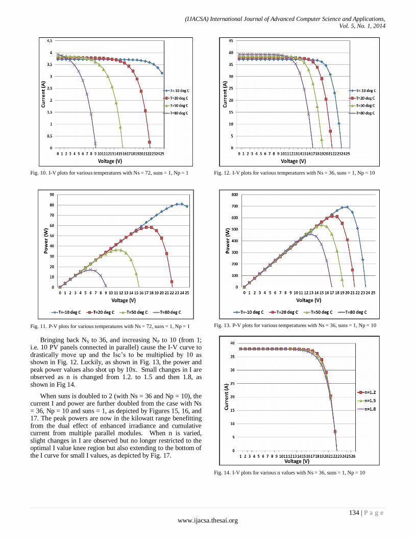
Bringing back suns to 1, and increasing NS to 72 (from 36) cause the gaps between the I-V curves at the different temperatures to widen and the I values to slightly drop at lower output voltage values, as shown in Fig. 10, and as compared to Fig. 4. These parameter changes also cause the maximum output powers to improve and rise slightly for T = -10 deg. Celsius. Unfortunately, maximum output powers drop for the higher temperatures 20-80 deg. Celsius, as shown in Fig. 11.




Fig. 11. P-V plots for various temperatures with Ns = 72, suns = 1, Np = 1

Bringing back NS to 36, and increasing NP to 10 (from 1; i.e. 10 PV panels connected in parallel) cause the I-V curve to drastically move up and the Isc’s to be multiplied by 10 as shown in Fig. 12. Luckily, as shown in Fig. 13, the power and peak power values also shot up by 10x. Small changes in I are observed as n is changed from 1.2. to 1.5 and then 1.8, as shown in Fig 14.

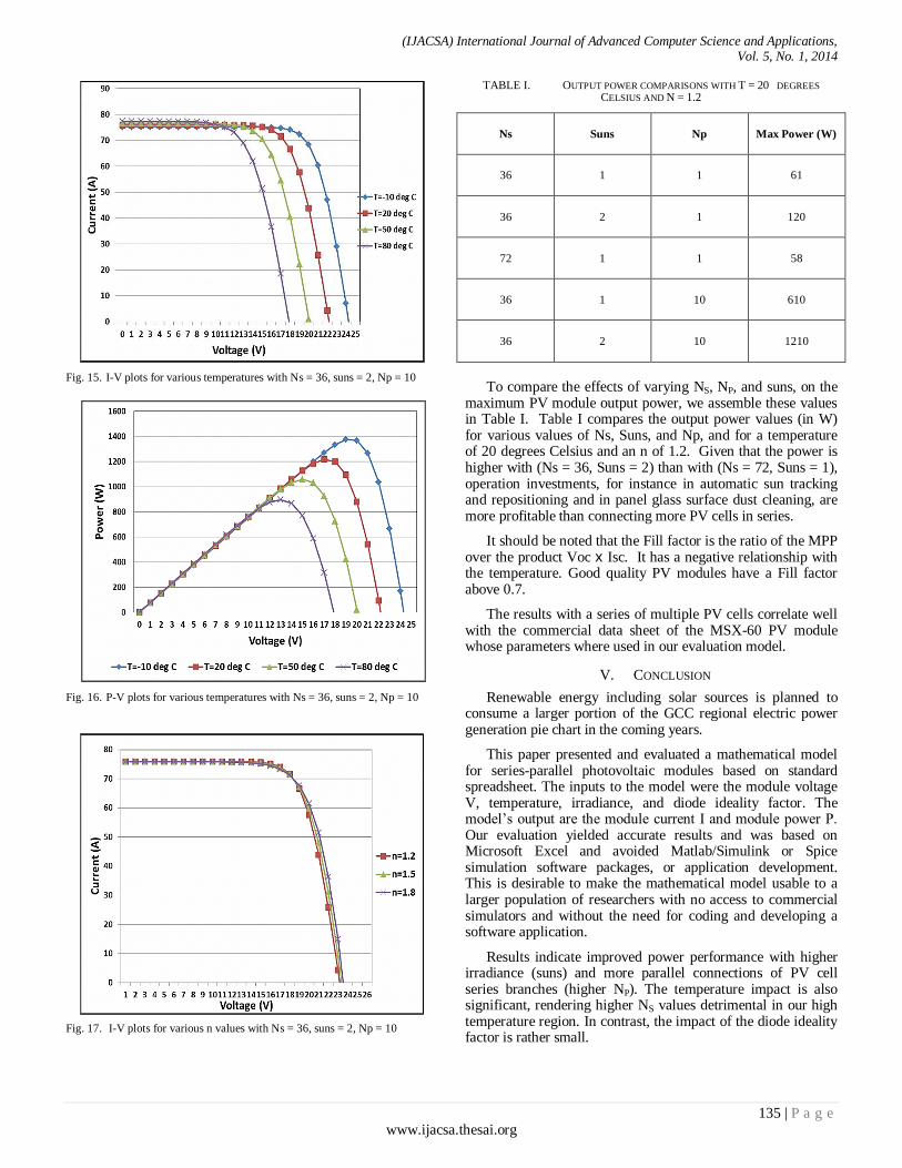
When suns is doubled to 2 (with Ns = 36 and Np = 10), the current I and power are further doubled from the case with Ns = 36, Np = 10 and suns = 1, as depicted by Figures 15, 16, and 17. The peak powers are now in the kilowatt range benefitting from the dual effect of enhanced irradiance and cumulative current from multiple parallel modules. When n is varied, slight changes in I are observed but no longer restricted to the optimal I value knee region but also extending to the bottom of the I curve for small I values, as depicted by Fig. 17.









TABLE I. OUTPUT POWER COMPARISONS WITH T = 20 DEGREES

CELSIUS AND N = 1.2

Ns

Suns

Np

Max Power (W)

36

1

1

61

36

2

1

120

72

1

1

58

36

1

10

610

36

2

10

1210

To compare the effects of varying NS, NP, and suns, on the

maximum PV module output power, we assemble these values in Table I. Table I compares the output power values (in W) for various values of Ns, Suns, and Np, and for a temperature of 20 degrees Celsius and an n of 1.2. Given that the power is higher with (Ns = 36, Suns = 2) than with (Ns = 72, Suns = 1), operation investments, for instance in automatic sun tracking and repositioning and in panel glass surface dust cleaning, are more profitable than connecting more PV cells in series.

It should be noted that the Fill factor is the ratio of the MPP over the product Voc x Isc. It has a negative relationship with the temperature. Good quality PV modules have a Fill factor above 0.7.

The results with a series of multiple PV cells correlate well with the commercial data sheet of the MSX-60 PV module whose parameters where used in our evaluation model.

V. CONCLUSION

Renewable energy including solar sources is planned to consume a larger portion of the GCC regional electric power generation pie chart in the coming years.

This paper presented and evaluated a mathematical model for series-parallel photovoltaic modules based on standard spreadsheet. The inputs to the model were the module voltage V, temperature, irradiance, and diode ideality factor. The model’s output are the module current I and module power P. Our evaluation yielded accurate results and was based on Microsoft Excel and avoided Matlab/Simulink or Spice simulation software packages, or application development. This is desirable to make the mathematical model usable to a larger population of researchers with no access to commercial simulators and without the need for coding and developing a software application.

Results indicate improved power performance with higher irradiance (suns) and more parallel connections of PV cell series branches (higher NP). The temperature impact is also significant, rendering higher NS values detrimental in our high temperature region. In contrast, the impact of the diode ideality factor is rather small.



Tracking mechanisms for repositioning the PV modules toward the sun’s rays and dust cleaning methods are therefore recommended to keep the PV module generating power near its MPP point. Given the hot weather in our region, increasing the number of cells connected in series (Ns) from 36 to 72 is not recommended.

As to future work, we may investigate dust cleaning options for PV modules and compare them based on output power performance, water requirements, and initial and long term costs.

ACKNOWLEDGMENT

We thank Saudi Aramco Management for authorizing the publication of this work.

REFERENCES

[1] J. A. Gow, and C. D. Manning, “Development of a photovoltaic array

model for use in power electronics simulation studies,” IEE Proceedings of Electric Power Applications, Vol. 146, No. 2, pp. 193–200, March

1999.

[2] K. H. Hussein, I. Muta, T. Hshino, and M. Osakada, “Maximum

photovoltaic power tracking: an algorithm for rapidly changing atmospheric conditions,” Proc. Inst. Elect. Eng, vol. 142, no. I, pp. 59-

64, Jan. 1995.

[3] J. Youngseok, S. Junghun, Y. Gwonjong and C. Jaeho, “Improved perturbation and observation method (IP&O) of MPPT control for

photovoltaic power systems,” Proc. 31st Photovoltaic Specialists Conference, Lake Buena Vista, Florida, pp. 1788 – 1791, January 2005.

[4] Nicola Femia, Giovanni Petrone, Giovanni Spagnuolo, and Massimo

Vitelli, “Optimization of perturb and observe maximum power point

tracking method,” IEEE Transactions on Power Electronics, vol. 20(4), pp. 963-973, 2005.

[5] G. Walker, “Evaluating MPPT converter topologies using a MATLAB PV model,” Journal of Electrical & Electronics Engineering, Australia,

IEAust, 21(1), pp. 49-56, 2001.

[6] Francisco M. Gonzalez-Longatt, “Model of photovoltaic module in Matlab,” 2 CIBELEC, 2005.

[7] T. DenHerder, Design and Simulation of Photovoltaic Super System

Using SIMULINK, Senior Project, Electrical Engineering Dept. California Polytechnic Univeristy, San Luis Obispo, 2006.

[8] H. Tsai, C. Tu, and Y. Su, “Development of generalized photovoltaic

model using MATLAB/SIMULINK,” Proc. World Congress on Engineering and Computer Science (WCECS 2008), Oct. 2008.

[9] F. Touati, M. Al-Hitmi, and H. Bouchech, “Towards understanding of

the effects of climatic and environmental factors on solar PV performance in arid desert regions (Qatar) for various PV technologies,”

Proc. First Int. Conference on Renewable Energies and Vehicular Technology, 2012.

[10] Gwinyai Dzimano, Modeling of Photovoltaic Systems, MS Thesis,

Electrical and Computer Engineering, Ohio State University, 2008.

[11] Mohamed Azab, “Improved circuit model of photovoltaic array,” Int.

Journal of Electrical Power and Energy Systems Engineering, vol. 2(3), 2009.

[12] D. Dondi, et al., “Photovoltaic cell modeling for solar energy powered

sensor networks,” Proc. 2nd IEEE International Workshop Advances in Sensors and Interface (IWASI 2007), 2007.

[13] M. Bouzguenda, A. Gastli, A. H. Al Badi, and T. Salmi, “Solar

photovoltaic inverter requirements for smart grid applications,” Proc. Innovative Smart Grid Technologies (ISGT)-Middle East, Jeddah, Saudi

Arabia, 2011.

Date post:	08-Dec-2015
Category:	Documents
Upload:	narasimha-prasad-tulasi
View:	214 times
Download:	0 times

MSX.60 series resistancepdf.pdf

Documents