MT5830 Hyperbolic Geometry Jonathan M. Fraser April 26, 2019 This work by Jonathan M. Fraser is licensed under a Creative Commons Attribution- NonCommercial-ShareAlike 4.0 International License. 1
Transcript
MT5830
Hyperbolic Geometry
Jonathan M. Fraser
April 26, 2019
This work by Jonathan M. Fraser is licensed under a Creative Commons Attribution-NonCommercial-ShareAlike 4.0 International License.
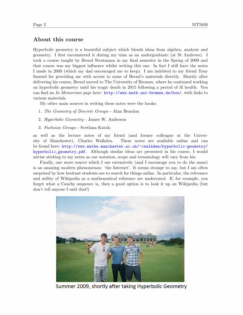
Hyperbolic geometry is a beautiful subject which blends ideas from algebra, analysis andgeometry. I first encountered it during my time as an undergraduate (at St Andrews). Itook a course taught by Bernd Stratmann in my final semester in the Spring of 2009 andthat course was my biggest influence whilst writing this one. In fact I still have the notesI made in 2009 (which my dad encouraged me to keep). I am indebted to my friend TonySamuel for providing me with access to some of Bernd’s materials directly. Shortly afterdelivering his course, Bernd moved to The University of Bremen, where he continued workingon hyperbolic geometry until his tragic death in 2015 following a period of ill health. Youcan find an In Memorium page here: http://www.math.uni-bremen.de/bos/, with links tovarious materials.
My other main sources in writing these notes were the books:
1. The Geometry of Discrete Groups - Alan Beardon
2. Hyperbolic Geometry - James W. Anderson
3. Fuchsian Groups - Svetlana Katok;
as well as the lecture notes of my friend (and former colleague at the Univer-sity of Manchester), Charles Walkden. These notes are available online and canbe found here: http://www.maths.manchester.ac.uk/~cwalkden/hyperbolic-geometry/hyperbolic_geometry.pdf. Although similar ideas are presented in his course, I wouldadvise sticking to my notes as our notation, scope and terminology will vary from his.
Finally, one more source which I use extensively (and I encourage you to do the same)is an amazing modern phenomenon: ‘the Internet’. It seems strange to say, but I am oftensurprised by how hesitant students are to search for things online. In particular, the relevanceand utility of Wikipedia as a mathematical reference are underrated. If, for example, youforget what a Cauchy sequence is, then a good option is to look it up on Wikipedia (butdon’t tell anyone I said that!)
Now, on to some mathematics... although don’t take anything I say in this section tooseriously; the course starts in Section 1! In this section I simply want to motivate the topic.
One of the oldest examples of axiomatic mathematics comes from Euclid’s postulates ongeometry in The Elements. These include seemingly harmless things like the ability to joinany two points by a straight line. In particular, the parallel postulate states:
“That, if a straight line falling on two straight lines make the interior angles on thesame side less than two right angles, the two straight lines, if produced indefinitely, meet onthat side on which are the angles less than the two right angles.”
It turns out that this postulate is rather interesting and in some sense defines Euclideangeometry (the geometry of Rn). In two dimensions, there are only three ‘possible geome-tries’, namely: Euclidean, spherical and hyperbolic (the third being the object of study inthis course). This is made precise by the uniformization theorem, which states than any sym-metric Riemann surface is conformally equivalent to the plane, the sphere or the disk. Twodimensional spherical geometry refers to the geometry of the surface of a sphere embeddedin R3. Here the ‘straight lines’ (distance minimising lines) are ‘great circles’ i.e. circles whichlie on the surface of the sphere and have the same diameter as the sphere itself (think of theequator lying on the surface of the earth). Already we see that the Parallel Postulate is introuble because any two great circles meet each other in two (antipodal) locations. This canbe interpreted as the non-existence of parallel lines in spherical geometry. Parallel lines areessentially unique in Euclidean geometry, in the sense that given a line and a point not onthat line, there is a unique line parallel to the given line passing through the given point.This is sometimes known as Playfair’s Axiom and is equivalent to the Parallel Postulate.Hyperbolic geometry fails in the opposite direction: given a line and a point not on that line,there there are (continuum) many lines parallel to the given line passing through the givenpoint! In particular, any Euclidean intuition you have concerning parallel lines may have togo out the window!
In higher dimensions, the situation gets rather more complicated. Compared to the three2-dimensional geometries, it turns out that there are eight 3-dimensional geometries. This
Page 4 MT5830
was essentially the concern of Thurston’s Geometrisation Conjecture, proved by Perelmanin 2003! Among many other things, the resolution of this problem implied the PoincareConjecture, which was one of the Millennium Problems presented by the Clay Institute in2000.
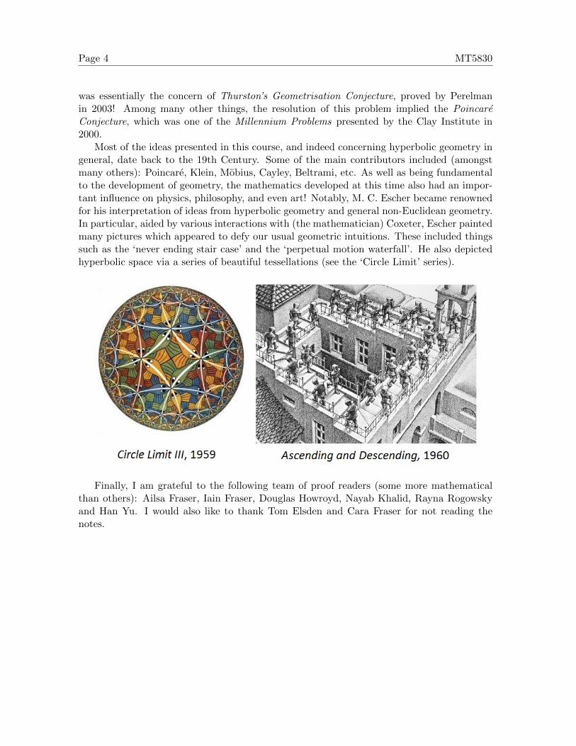
Most of the ideas presented in this course, and indeed concerning hyperbolic geometry ingeneral, date back to the 19th Century. Some of the main contributors included (amongstmany others): Poincare, Klein, Mobius, Cayley, Beltrami, etc. As well as being fundamentalto the development of geometry, the mathematics developed at this time also had an impor-tant influence on physics, philosophy, and even art! Notably, M. C. Escher became renownedfor his interpretation of ideas from hyperbolic geometry and general non-Euclidean geometry.In particular, aided by various interactions with (the mathematician) Coxeter, Escher paintedmany pictures which appeared to defy our usual geometric intuitions. These included thingssuch as the ‘never ending stair case’ and the ‘perpetual motion waterfall’. He also depictedhyperbolic space via a series of beautiful tessellations (see the ‘Circle Limit’ series).
Finally, I am grateful to the following team of proof readers (some more mathematicalthan others): Ailsa Fraser, Iain Fraser, Douglas Howroyd, Nayab Khalid, Rayna Rogowskyand Han Yu. I would also like to thank Tom Elsden and Cara Fraser for not reading thenotes.
Page 5 MT5830
1 Introduction and some preliminaries
One of the underlying themes of this course is the interplay between the geometry of a metricspace and the group of transformations which preserve the metric (group of isometries).Broadly speaking, one may think of ‘geometry’ as the study of invariants under a fixed groupof transformations. In our setting the invariant will be the hyperbolic metric, but one maystudy any metric space in this way, or indeed study other (non-metric) invariants. In thissection we will recall and discuss some of the basic concepts we will rely on throughout thecourse, such as metric spaces, isometries, groups, and group actions.
As with many areas of pure mathematics, we will usually begin with a space X, whichis just a non-empty set. We are then interested in adding structure to the space (which atthe moment is quite boring, at least from a geometers point of view). A metric is a functionwhich allows us to measure the distance between two points in our space and the definitionsimply ensures that the function is a sensible choice.
Definition 1.1. A metric space is a non-empty set X together with a metric d : X×X → Rsuch that
1. (positivity) ∀x, y ∈ X : d(x, y) > 0
2. (identity of indiscernibles) ∀x, y ∈ X : d(x, y) = 0⇔ x = y
3. (symmetry) ∀x, y ∈ X : d(x, y) = d(y, x)
4. (triangle inequality) ∀x, y, z ∈ X : d(x, y) 6 d(x, z) + d(z, y)
An important example to keep in mind at this point is Euclidean space Rn with theusual Euclidean metric d(x, y) = |x − y|. In ‘reasonable’ metric spaces, one can ask thequestion: ‘what is the most efficient way to travel between two points of the space?’ In thiscontext ‘efficient’ means distance minimising in a sense we will make precise. For example,in Euclidean space the most efficient way to travel between two points is via the (unique)straight line joining the two points.
Definition 1.2. Let (X, d) be a metric space and let x, y ∈ X with x 6= y. A set (curve)C ⊆ X is called a geodesic (from x to y) if there exists a continuous bijection γ : [0, 1]→ Csuch that
1. γ(0) = x and γ(1) = y
2. for all s, t ∈ [0, 1] we have
d(γ(s), γ(t)) = d(x, y)|s− t|.
Now that we have additional structure on our space we can look for transformations whichpreserve this structure. Such transformations are called isometries.
Page 6 MT5830
Definition 1.3. Let (X, d) be a metric space. A transformation φ : X → X is an isometryif
1. φ is a bijection
2. ∀x, y ∈ X : d(φ(x), φ(y)) = d(x, y)
Continuing our example from before, the isometries of Euclidean space are precisely mapsof the form
φ(x) = t+Ax
where t ∈ Rn is a translation and A is an orthogonal matrix, i.e. an n × n matrix over Rsuch that AAT = ATA = I.
The collection of all isometries of a metric space is an interesting object in its own right.First of all, note that it is always non-empty and if one composes two isometries, then onegets an isometry back again. This means that the collection of all isometries has an elegantalgebraic structure.
Definition 1.4. A group is a set X together with a binary operation which takes a pair(x, y) ∈ X ×X to another element in X, denoted by x · y, which satisfies
1. (associativity) ∀x, y, z ∈ X : x · (y · z) = (x · y) · z
2. (identity) ∃e ∈ X : ∀x ∈ X : x · e = e · x = x
3. (inverses) ∀x ∈ X : ∃y ∈ X : x · y = y · x = e
The key fact to take away from this section is the following:
Theorem 1.5. Given any metric space, the collection of all isometries forms a group wherethe binary operation is composition of maps. This group is sometimes called the group ofisometries (of the metric space).
Composition of maps is very simple However, be careful in which direction you are com-posing! Given maps φ1, φ2 : X → X, the composition φ1 ◦ φ2 : X → X is defined by
φ1 ◦ φ2(x) = φ1(φ2(x))
i.e. we are composing from right to left (apply φ2 first, then apply φ1). We say that thegroup of isometries acts on the metric space X and the action of an isometry φ on an elementx ∈ X is given by φ(x).
The group of isometries of Euclidean space is called the Euclidean group and is given bya semidirect product of Rn (where the group operation is vector addition) and O(n,R), thegroup of real n× n orthogonal matrices. More precisely, the Euclidean group is
E(n) ∼= O(n,R) nRn
where the semidirect product is the direct product O(n,R) × Rn equipped with the skew-product operation
(A1, t1) · (A2, t2) = (A1 ◦A2, A1(t2) + t1).
(We will not deal with semidirect products in this course, and so this description is merelyan aside). Another important group to mention at the moment is the general linear group
Page 7 MT5830
GL(n,R), which consists of all real n × n invertible matrices. Also, the special linear groupSL(n,R), which consists of all real n × n matrices with determinant 1. Thus we have thefollowing subgroup hierarchy
SO(n,R) 6 SL(n,R) 6 GL(n,R),
where SO(n,R) 6 O(n,R) is the special orthogonal group, which is the set of orientationpreserving orthogonal matrices (those with determinant 1). A common theme in group theory(and related areas) is to consider the following question: once you have a group, can you writedown a simple collection of elements which can be used to build all the elements of the group?
Definition 1.6. Given a group X and a collection of elements A ⊆ X, the subgroup gener-ated by A is written 〈A〉 6 X and is defined to be the smallest subgroup of X containing A,i.e.
〈A〉 =⋂
A⊆Z6XZ.
A beautiful fact from elementary group theory is that 〈A〉 is precisely the set of elementswhich can be written as finite products of elements from A and their inverses. The Euclideangroup is generated by reflections in straight lines (infinite extensions of geodesics).
Finally, we end this introduction by recalling the hyperbolic trig functions, which will berelevant for this course. For x ∈ R we have
sinh(x) =ex − e−x
2and cosh(x) =
ex + e−x
2.
Rather than stating various identities concerning these functions, we just emphasise that theyall follow from the definitions and you should be ready to derive them when necessary!
Page 8 MT5830
2 The Poincare disk model of hyperbolic space
2.1 The hyperbolic metric
We are about to meet our first model of hyperbolic space and the hyperbolic metric. Thespace will be something rather familiar: the interior of the unit disk in the complex plane.In particular, we will refer to the Poincare disk
D2 = {z ∈ C : |z| < 1}
and the boundaryS1 = {z ∈ C : |z| = 1} = D2 \ D2.
Of course, the Poincare disk may be equipped with the Euclidean metric and in this settingit is not difficult to see that its group of isometries is isomorphic to O(2,R) (rotations andreflections). Thus the group of isometries of the disk is a proper subgroup of the group ofisometries of the plane due to the fact that there is ‘no room’ for translations. However, wewill put a metric on the disk which recovers the ‘room’ present in the whole plane. Clearlythis metric will have to be very non-Euclidean. The key idea is that as one approaches theboundary S1 the metric will ‘blow-up’ in comparison to the Euclidean metric. In other words,moving towards the boundary of the disk will be like moving off to infinity in the plane. Forthis reason S1 is sometimes called the boundary at infinity.
Consider the following ‘hyperbolic kernel’ h : D2 → R defined by
h(z) =2
1− |z|2.
Notice that h(z) blows up as z approaches the boundary. Let γ : [0, 1]→ D2 be a continuousinjection given by
γ(t) = α(t) + iβ(t)
where we assume that α and β are differentiable with continuous derivatives α′ and β′. Thusγ defines a curve C = γ([0, 1]) ⊂ D2 in the Poincare disk and we may compute the length ofthe curve with respect to the hyperbolic kernel as
L(C) =
∫Ch(z)|dz| =
∫C
2 |dγ(t)|1− |γ(t)|2
=
∫ 1
0
2√α′(t)2 + β′(t)2
1− (α(t)2 + β(t)2)dt.
This integral looks unpleasant at first sight, but just think of it as the standard ‘length’ of asmooth curve distorted by the hyperbolic kernel. We are now ready to define the hyperbolicmetric. For w, z ∈ D2 we say C is a continuously differentiable curve joining w, z if C isparameterised by a function γ as above and γ(0) = w and γ(1) = z. The hyperbolic distancebetween w, z is defined by
dD2(w, z) = inf{L(C) : C is a continuously differentiable curve joining w, z}.
Again, this looks rather unpleasant at first sight, and not particularly easy to work with!However, as is often the case with complicated abstract objects, we will rarely work directlyfrom this definition. Instead we will derive elementary formulae for the distances betweenparticular points and then explore the metric via its geodesics, isometries, and characteristicfeatures! We will spend the rest of the course trying to understand this beautiful metric andthe geometry it creates.
It should be clear that dD2 satisfies all the conditions of being a metric. Perhaps, themost subtle is ‘identity of indiscernibles’, but this will be dealt with explicitly later.
Page 9 MT5830
2.2 The group of isometries
Our first task will be to identify the isometry group of the metric space (D2, dD2). This turnsout to be the collection of all conformal automorphisms of the disk, i.e., angle preservingbijections from the disk to itself. This group has the following simple description:
con(1) =
{g : D2 → D2 : for some a, c ∈ C with |a|2 − |c|2 = 1
g(z) =az + c
cz + afor all z ∈ D2 or
g(z) =az + c
cz + afor all z ∈ D2
}The distinction between the first and second ‘standard form’ is simply that the first preservesorientation and the second reverses it. We will write the subgroup consisting of all orientationpreserving elements of con(1) as con+(1). In fact con+(1) is a subgroup of a very importantgroup of transformations acting on the extended complex plane C = C ∪ {∞}, known as theMobius group given by
Mob+ =
{g : C→ C : for some a, b, c, d ∈ C with ad− bc 6= 0
g(z) =az + b
cz + dfor all z ∈ C
}.
Elements of Mob+ are known as Mobius maps or Mobius transformations. Note that weadopt the convention that, for a Mobius map g, g(∞) = a/c ∈ R if c 6= 0 and ∞ otherwiseand g(0) = b/d ∈ R if d 6= 0 and ∞ otherwise. The following fact about Mob+ is a classicalresult from complex analysis which we will use but not prove.
Theorem 2.1. Mobius maps are holomorphic bijections from the Riemann sphere (identifiedwith C) to itself with non-zero derivative. In particular, they are conformal, which meansthey preserves angles locally.
The main message from this theorem is that Mobius maps preserve angles. In particular,if two differentiable curves meet at some angle (defined by their tangents at the point ofintersection), then the image of these curves under a Mobius map intersect at the sameangle.
The following key property will be used throughout the course.
Lemma 2.2. The image of a (doubly infinite) straight line or a circle under a Mobius mapis either a (doubly infinite) straight line or a circle.
Proof. The proof follows a standard decomposition argument. Given g ∈ Mob+, we canrewrite g(z) as follows
g(z) =
{adz + b
d if c = 0bc−adc2
1z+d/c + a
c if c 6= 0.
This shows that if c = 0 then g is the composition of a rotation, a dilation and a translation.Also, if c 6= 0 then g is the composition of the maps:
Page 10 MT5830
• z 7→ z + d/c (a translation)
• z 7→ 1z (a circle inversion composed with a reflection)
• z 7→ bc−adc2
z (a rotation combined with a dilation)
• z 7→ z + ac (a translation).
Clearly, translations, rotations and dilations send straight lines to straight lines and circlesto circles. Perhaps surprisingly this is also almost true for circle inversions. In particular, wewill show that the inversion z 7→ 1/z sends lines and circles to lines and circles. Thereforethis is also true of elements in Mob+.
First we will show that circles and straight lines in C can be expressed in a similar form.First, points z = x+ iy on a straight line always satisfy
ax+ by + c = 0
for some a, b, c ∈ R. This is equivalent to
a
2(z + z) +
b
2i(z − z) + c = 0
and, setting B = a/2 + b/(2i) and C = c, yields
Bz +Bz + C = 0.
Second, points z on a circle centred at u ∈ C with radius r satisfy
|z − u|2 = (z − u)(z − u) = r2.
This yieldszz − zu− uz + |u|2 = r2
and, setting A = 1, B = −u and C = |u|2 − r2, we get
Azz +Bz +Bz + C = 0.
Thus, this is the general equation for a circle or a straight line, where B ∈ C, C ∈ R andA ∈ {0, 1} with A = 0 corresponding to lines and A = 1 corresponding to circles.
Therefore if z 6= 0 lies on the circle or line corresponding to A,B,C, then dividing by zzwe obtain
C1
zz+B
1
z+B
1
z+A = 0.
If C = 0 this shows that 1/z lies on the line corresponding to the data “B” = B, “C” = A.If C 6= 0, then further dividing by C shows that 1/z lies on the circle corresponding to thedata “A” = 1, “B” = B/C, “C” = A/C. Recall that C is real. We deduce that the image ofa circle or a straight line under the inversion z 7→ 1/z is a circle or a straight line.
Let us note that some ‘obvious’ isometries are clearly present in con(1):
1. the identity: choose a = 1 and c = 0 then
g(z) =1z + 0
0× z + 1= z
is a member of con(1).
Page 11 MT5830
2. rotation by an angle θ: choose a = exp(iθ/2) and c = 0 then
g(z) =exp(iθ/2)z + 0
0× z + exp(iθ/2)=
exp(iθ/2)z
exp(−iθ/2)= exp(iθ)z
is a member of con(1).
3. reflection in the real axis (conjugation): choose a = 1 and c = 0 then
g(z) =1z + 0
0× z + 1= z
is a member of con(1).
4. reflection in any straight line through the origin: this can be built as the compositionof rotations and conjugation.
Theorem 2.3. The elements of con(1) form a group. Moreover con(1) is generated bycon+(1) together with the conjugation map z 7→ z.
Proof. See the tutorial questions.
We are almost ready to prove that all elements in con(1) are isometries of (D2, dD2). Webegin with a simple technical lemma concerning the derivative of elements in con+(1).
Lemma 2.4. For g ∈ con+(1) we have
|g′(z)| = 1− |g(z)|2
1− |z|2.
Proof. Let g ∈ con+(1) be given by
g(z) =az + c
cz + a
for some a, c ∈ C with |a|2 − |c|2 = 1. Using the quotient-rule, we have
|g′(z)| =∣∣∣∣a(cz + a)− c(az + c)
(cz + a)2
∣∣∣∣ =|a|2 − |c|2
|cz + a|2=
1
|cz + a|2.
On the other hand we have
1− |g(z)|2 = 1−∣∣∣∣az + c
cz + a
∣∣∣∣2=|cz + a|2 − |az + c|2
|cz + a|2
=(cz + a)(cz + a)− (az + c)(az + c)
|cz + a|2
=(|a|2 − |c|2)(1− |z|2)
|cz + a|2
=1− |z|2
|cz + a|2.
Putting these two estimates together yields the desired result.
Page 12 MT5830
Theorem 2.5. The elements of con(1) are isometries of (D2, dD2), i.e. for g ∈ con(1) andu, v ∈ D2 we have
dD2(u, v) = dD2(g(u), g(v)).
Proof. Let g ∈ con+(1) and let C be a continuously differentiable curve joining u and v.Using the substitution z = g(w) and the previous lemma we have
L(g(C)) =
∫g(C)
2
1− |z|2|dz| =
∫C
2
1− |g(w)|2|g′(w)||dw|
=
∫C
2
1− |g(w)|21− |g(w)|2
1− |w|2|dw|
=
∫C
2
1− |w|2|dw|
= L(C).
It follows from the chain rule that g ∈ con+(1) maps continuously differentiable curves Cjoining u and v to continuously differentiable curves g(C) joining g(u) and g(v). Therefore
dD2(u, v) = infCL(C) = inf
CL(g(C)) = inf
g(C)L(g(C)) = dD2(g(u), g(v)).
which complete the proof for g ∈ con+(1). However, since elements in con(1) can be obtainedby composition of maps in con+(1) and conjugation (which is obviously an isometry), we mayconclude the result in full generality.
The above theorem does not quite say that the isometry group of the Poincare disk iscon(1). It only says that the isometry group contains con(1). However, it turns out that itis precisely the isometry group. We will use this fact, but omit the proof. A proof can befound in Anderson (Proposition 4.2) for example.
2.3 Hyperbolic geodesics
Our next task is to get a better handle on the metric dD2 . We begin by deriving a simple butimportant formula. Notice how we use the fact that con(1) is the isometry group.
Lemma 2.6. For z ∈ D2 we have
dD2(0, z) = log1 + |z|1− |z|
.
Proof. Let z ∈ D2 and write it in polar form as z = |z|eiθ. We begin by making use of con(1)to simplify the problem. Let g ∈ con(1) be given by
g(w) = e−iθw.
Recall we have already seen that such rotations are members of con+(1). Since g is anisometry we have
dD2(0, z) = dD2(gθ(0), gθ(z)) = dD2(0, |z|).
Page 13 MT5830
Now let C be a continuously differentiable curve joining 0 and |z| parameterised by γ. Thenγ can be decomposed into real part and imaginary part, that is γ(t) = α(t) + iβ(t) for real-valued functions α, β : [0, 1]→ R such that α(0) = β(0) = β(1) = 0 and α(1) = |z|. We thenhave
L(C) =
∫ 1
0
2√α′(t)2 + β′(t)2
1− (α(t)2 + β(t)2)dt >
∫ 1
0
2√α′(t)2
1− α(t)2dt
=
∫ 1
0
2α′(t) dt
1− α(t)2
=
∫ |z|0
2 du
1− u2(setting u = α(t))
=
[log
1 + u
1− u
]|z|0
= log1 + |z|1− |z|
proving one direction of the desired result. However, the other direction is simple. Thereis only one place where we get an inequality rather than an equality and it is easily seenthat equality holds here if and only if β(t) = 0 ∀t ∈ [0, 1]. This means that the curve whichminimises L(C) must be the Euclidean straight line between 0 and z. Therefore,
dD2(0, z) = infγL(γ([0, 1])) = log
1 + |z|1− |z|
as required.
We can use the formula from the previous lemma and the con(1) invariance to deriveother formulae for the hyperbolic distance between two points.
Corollary 2.7. The following useful formulae hold for all z, w ∈ D2.
1. dD2(z, w) = log |1−zw|+|z−w||1−zw|−|z−w|
2. cosh dD2(z, w) = |1−zw|2+|z−w|2|1−zw|2−|z−w|2
3. sinh2 dD2 (z,w)
2 = |z−w|2(1−|z|2)(1−|w|2)
.
Proof. Let z, w ∈ D2 and define gw ∈ con(1) by
gw(u) =
i√1−|w|2
u+ −iw√1−|w|2
iw√1−|w|2
u+ −i√1−|w|2
.
One can check that gw is indeed in con(1), and that gw(w) = 0. Therefore
The formulae in 2. and 3. follow immediately by inserting 1. into
cosh dD2(z, w) =edD2 (z,w) + e−dD2 (z,w)
2and sinh2 dD2(z, w)
2=edD2 (z,w) + e−dD2 (z,w) − 2
4
and simplifying.
Note that this corollary finally establishes that dD2 is a metric, by showing it satisfies‘identity of indiscernibles’ !
The next result is both aesthetically pleasing and fundamental to understanding thegeometry of D2.
Theorem 2.8. Hyperbolic geodesics exist and are unique between any two points in D2.Moreover, they either lie on Euclidean straight lines through the origin or on circles in D2
orthogonal to S1 (that is C ∩ D2, where C is a circle orthogonal to S1).
Proof. We have already seen that geodesics between 0 and a point z ∈ D2 exist and are unique.This extends to any two points u, v ∈ D2 by the following simple observation. Consider theelement
gu(z) =
i√1−|u|2
z + −iu√1−|u|2
iu√1−|u|2
z + −i√1−|u|2
.
Note that gu in con+(1), and note that gu(u) = 0. It is then straightforward to showthat the (unique) geodesic between 0 and gu(v) maps to a geodesic between u and v viag−1u ∈ con+(1). Also if there were two different geodesics between u and v, then these would
map to two different geodesics between 0 and gu(v) via gu which would be a contradiction.We have therefore shown that any geodesic is the image of a straight line emanating from
the origin under some g ∈ con(1). Therefore, since g is a Mobius transformation, we knowthat it lies on a circle or a straight line which intersects S1 at right angles.
Page 15 MT5830
2.4 OK, that’s all very nice...
At this point I think it is important to discuss some motivation for this subject. So farwe have seen some of the beautiful geometric properties of hyperbolic space. The fact thatgeodesics lie on circles intersecting the boundary at right angles is particularly pleasing!However, all of this follows from our choice of hyperbolic kernel. In particular, we couldhave chosen a different kernel: any strictly increasing continuous function f : [0, 1)→ (0,∞)with the property that f(x) → ∞ as x → 1 would lead to a similar effect if we had chosenthe kernel to be z 7→ f(|z|), although the geometry would not be so beautiful (perhaps?).So what is so special about the hyperbolic kernel and was it just chosen to make prettypictures? The answer is that the hyperbolic kernel and resulting geometry is very special.One can think of kernels which blow up at the boundary as adding ‘negative curvature’ tothe (usually ‘flat’) complex disk. A good way to visualise this is to imagine the hyperbolicdisk as the inside of a cereal bowl. If an ant was to start in the middle and walk to the edgeit would find that it needs to make increasingly more effort as it gets nearer to the edge dueto the (negative) curvature of the bowl. Whereas walking on the surface of a sphere presentsdifferent geometric features due to the (positive) curvature of the sphere. There is a rigorousabstract definition of ‘curvature’ which can be applied to smooth manifolds and if one wantsto study negatively curved spaces then one might ask the following question: what are thesymmetric, simply connected, 2-dimensional Riemannian manifolds with constant negativecurvature? (The natural question, don’t you agree? :-) ) The answer is that there is onlyone, and it is the hyperbolic space we have just constructed! The concepts I have hinted atin this section will not play a role in this course apart from motivating the model. However,the important heuristic to take away is that the hyperbolic kernel was chosen to guaranteeconstant negative curvature. Different kernels would not have achieved this.
2.5 Hyperbolic triangles
Euclidean triangles are some of the first geometric objects we learn about. We learn theoremslike Pythagoras’ theorem, various results in trigonometry, and formulae for the area. Moreabstractly, provided your metric space has unique geodesics, one may define triangles to bethe area enclosed by the three geodesics joining three distinct points in the space which do notall lie on a single geodesic (if the three points are collinear, then the triangle is degenerate).Unsurprisingly, the geometry of hyperbolic triangles (i.e. triangles formed by geodesics inD2) is rather different from the Euclidean case. However, we already know what they looklike, because we understand geodesics.
Page 16 MT5830
Here is the hyperbolic analogue of Pythagoras’ theorem.
Theorem 2.9. For every right angled hyperbolic triangle in D2 with hypotenuse of hyperboliclength c, and remaining sides of hyperbolic length a and b, we have
cosh c = cosh a cosh b.
Proof. Since con(1) consists of angle-preserving isometries of D2, we can assume without lossof generality that 0 is the vertex opposite the hypotenuse, and that the remaining verticesare at α (corresponding to a) and at iβ (corresponding to b), for α, β ∈ (0, 1). Otherwise wecould move the triangle to this special triangle without changing any distances! We have
cosh c = cosh dD2(α, iβ) =|1− αiβ|2 + |α− iβ|2
|1− αiβ|2 − |α− iβ|2
=|1 + iαβ|2 + |α− iβ|2
|1 + iαβ|2 − |α− iβ|2
=1 + α2β2 + α2 + β2
1 + α2β2 − α2 − β2
=(1 + α2)(1 + β2)
(1− α2)(1− β2)
= cosh dD2(0, α) cosh dD2(0, iβ)
= cosh a cosh b
as required.
If a, b, c are the lengths of a sides of a triangle (in any metric space), then we alwayshave c 6 a + b (this is just the triangle inequality!) Consider a right angled Euclideanisosceles triangle with two sides of length a and the hypotenuse of length c. Then the classicalPythagoras’ theorem tells us that c =
√2a, which tells us that in general the reverse of the
triangle inequality can fail by a multiplicative constant, i.e.
1√2
(a+ a) = c =√
2a 6 a+ a.
This is not the case in hyperbolic space and in fact the reverse of the triangle inequality onlyfails by an additive constant for right angled triangles (think about the difference betweenmultiplicative and additive in this setting).
Corollary 2.10. For every right angled hyperbolic triangle in D2 with hypotenuse of hyper-bolic length c, and remaining sides of hyperbolic length a and b, we have
a+ b− 2 log 2 6 c 6 a+ b.
Proof. By the triangle inequality we only have to prove the first inequality. Observe that forx > 0 we have
1
2ex 6 coshx 6 ex,
and hencex− log 2 6 log coshx 6 x.
Page 17 MT5830
Using this general observation, the previous theorem implies
An archetypal feature of hyperbolic space is that it has thin triangles. Generally speaking,a geodesic metric space is called δ-hyperbolic (not really the same use of the word ‘hyperbolic’)if it has thin triangles, i.e. there exists δ > 0 such that for any triangle the distance fromat least one of the sides to the opposite vertex is less than δ. Check to see that this fails forEuclidean triangles! Generally, if (X, d) is a metric space and x ∈ X is a point and C ⊂ Xis a subset (the side of a triangle for example), then the distance from x to C is given by
d(x,C) = infy∈C
d(x, y).
Corollary 2.11. Consider a right angled hyperbolic triangle in D2. If P is the vertex oppositethe hypotenuse, then the hyperbolic distance from P to the hypotenuse is always bounded by3 log 2.
Proof. As in the proof of the previous theorem we can assume without loss of generalitythat our triangle is of the type considered in that proof. Let L be the straight line from0 which intersects the hypotenuse of the triangle at right angles. This line naturally splitsthe hypotenuse into 2 parts which we will label as having lengths ca (the part joining α)and cb (the part joining β). In particular, since the sides of a triangle are geodesics we havec = ca + cb and moreover the line L splits the original triangle into two smaller right angledtriangles. To prove the result it will be sufficient to estimate the length of the line L whichwe denote by δ. By applying the previous theorem to the original triangle and the two newtriangles we obtain:
ca + δ − 2 log 2 6 a 6 ca + δ,
cb + δ − 2 log 2 6 b 6 cb + δ
anda+ b− 2 log 2 6 c 6 a+ b.
Adding the first to the second and then applying the third we obtain
c+ 2δ 6 a+ b+ 4 log 2 6 c+ 6 log 2.
Canceling c and dividing by 2 completes the proof. If this proof was confusing at all, thendraw a picture!
Page 18 MT5830
2.6 Hyperbolic circles
Hyperbolic circles are also very different from Euclidean circles. However, they have a pleas-ingly straightforward shape: they are Euclidean circles! This similarity and the importantdifferences will become clear throughout this section. We begin by comparing Euclidean andhyperbolic circles centred at 0. For z ∈ D2 and r > 0, we write
CD2(z, r) = {w ∈ D2 : dD2(z, w) = r}
for the hyperbolic circle centred at z with radius r and
CE(z, r) = {w ∈ D2 : |z − w| = r}
for the Euclidean circle centred at z with radius r.
Theorem 2.12. For any radius r > 0 we have
CD2(0, r) = CE(0, tanh(r/2)).
Proof. Suppose z ∈ D2 is such that dD2(0, z) = r. Using the basic formulae we derived aboveit follows that
r = log1 + |z|1− |z|
and by rearranging this formula for |z| we obtain
|z| = er − 1
er + 1= tanh(r/2)
as required.
This result shows us that hyperbolic circles centred at the origin look exactly like Eu-clidean circles centred at the origin. Since we know the hyperbolic metric is invariant underrotations of D2 this should not be surprising! We can actually say more simply by using thefact that elements of con(1) send circles to circles (or straight lines).
Theorem 2.13. Hyperbolic circles in D2 are Euclidean circles and vice versa (although thecentres are different unless at the origin).
Proof. Let C be a Euclidean circle centred at z ∈ D2. Let L denote the (infinite) straight linepassing through 0 and the centre of C. This line intersects C at right angles in two points,which we denote by u and v. Moreover, we know that the geodesic between u and v lies onthe line L. Let w be the hyperbolic midpoint of this geodesic and let g ∈ con(1) be suchthat g(w) = 0. We know g(C) must be a Euclidean circle since g cannot map C to a straightline in this case (think about why this is). Moreover this circle must be centred at the originsince g(L) must be a line passing through g(u), g(w) = 0 and g(v) intersecting g(C) at rightangles with 0 being the midpoint of the geodesic joining g(u) and g(v). Therefore by theprevious theorem it is also a hyperbolic circle. It follows that C = g−1(g(C)) is a hyperboliccircle, centred at w.
In the opposite direction, let C be a hyperbolic circle centred at z ∈ D2. We do nota priori know what C looks like. Let g ∈ con(1) be such that g(z) = 0. Then g(C) is ahyperbolic circle centred at the origin and is therefore a Euclidean circle. It follows thatC = g−1(g(C)) is a Euclidean circle.
Page 19 MT5830
It is somewhat of a relief that hyperbolic circles are Euclidean circles as this makes themrather simple to visualise. However, they behave very differently! We will demonstrate thisby comparing two important quantities: circumference and area. For z ∈ D2 and r > 0, wewrite
BD2(z, r) = {w ∈ D2 : dD2(w, z) 6 r}
andBE(z, r) = {w ∈ D2 : |z − w| 6 r}
for the hyperbolic and Euclidean ball respectively. Recall that the (Euclidean) circumferenceof a Euclidean circle is given by the familiar formula
LE(CE(z, r)) = 2πr
and the (Euclidean) area of a Euclidean ball is given by the familiar formula
AE(BE(z, r)) = πr2.
The hyperbolic area of a ‘reasonable’ set F is given by
AD2(F ) =
∫Fh(z)2|dz| =
∫F
4
(1− |z|2)2|dz|.
Here ‘reasonable’ refers to a technical integrability condition, which we will not worry about.Certainly ‘reasonable’ includes any area enclosed by piecewise differentiable curves for exam-ple and we will not compute the area of anything that does not fall into this category.
Importantly (and unsurprisingly) hyperbolic area is preserved by con(1).
Theorem 2.14. Let F ⊂ D2 be ‘reasonable’. Then for all g ∈ con(1) we have
AD2(F ) = AD2(g(F )).
Proof. This is similar to the proof that con(1) preserves hyperbolic length and is left as anexercise on the tutorial sheets.
Theorem 2.15. For all hyperbolic circles CD2(z, r) of radius r, we have
LD2(CD2(z, r)) = 2π sinh r.
Proof. This is in the tutorial sheets.
As r becomes very large the circumference of a hyperbolic circle grows exponentially inr. More precisely, we have
LD2(CD2(z, r)) = 2π sinh r = 2πer − e−r
2∼ πer
as r → ∞. Here A ∼ B as a parameter x → ∞ formally means that A/B → 1 as x → ∞.This is very different from the Euclidean situation where the circumference grows linearly!
Theorem 2.16. For all hyperbolic balls BD2(z, r) of radius r, we have
AD2(BD2(z, r)) = 4π sinh2 r
2.
Page 20 MT5830
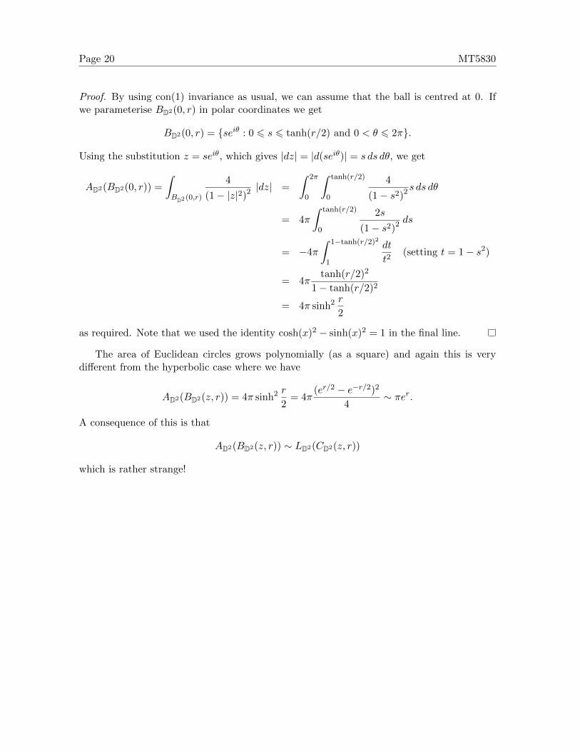
Proof. By using con(1) invariance as usual, we can assume that the ball is centred at 0. Ifwe parameterise BD2(0, r) in polar coordinates we get
BD2(0, r) = {seiθ : 0 6 s 6 tanh(r/2) and 0 < θ 6 2π}.
Using the substitution z = seiθ, which gives |dz| = |d(seiθ)| = s ds dθ, we get
AD2(BD2(0, r)) =
∫BD2 (0,r)
4
(1− |z|2)2 |dz| =
∫ 2π
0
∫ tanh(r/2)
0
4
(1− s2)2 s ds dθ
= 4π
∫ tanh(r/2)
0
2s
(1− s2)2 ds
= −4π
∫ 1−tanh(r/2)2
1
dt
t2(setting t = 1− s2)
= 4πtanh(r/2)2
1− tanh(r/2)2
= 4π sinh2 r
2
as required. Note that we used the identity cosh(x)2 − sinh(x)2 = 1 in the final line.
The area of Euclidean circles grows polynomially (as a square) and again this is verydifferent from the hyperbolic case where we have
AD2(BD2(z, r)) = 4π sinh2 r
2= 4π
(er/2 − e−r/2)2
4∼ πer.
A consequence of this is that
AD2(BD2(z, r)) ∼ LD2(CD2(z, r))
which is rather strange!
Page 21 MT5830
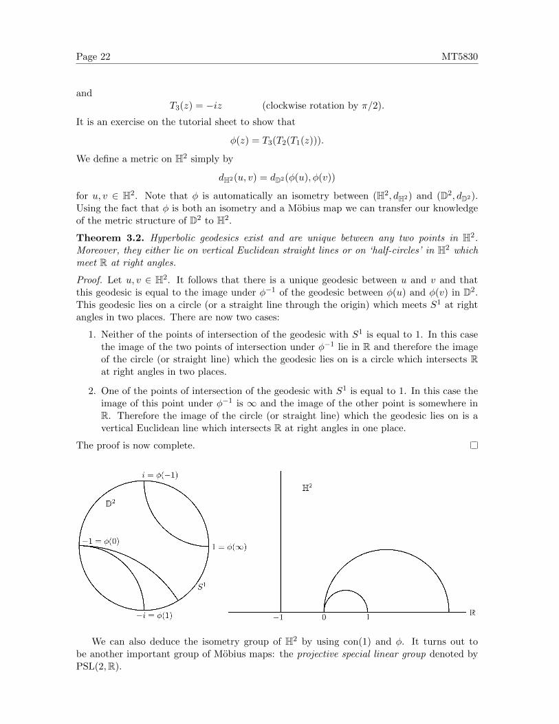
3 The upper half-plane model of hyperbolic space
So far we have been working in the metric space (D2, dD2), which is one model of 2-dimensionalhyperbolic space. However, it is not the only model of this important space, as we shall seein this section. Understanding and describing different models is important because someproblems are more easily understood in one model, over another. This time our ambientspace will be the upper half-plane
H2 = {z ∈ C : Im(z) > 0} = {x+ iy : y > 0}
and this time the ‘boundary at infinity’ will be the one point compactification of the real linegiven by
R = R ∪ {∞}.
We could now write down an appropriate ‘hyperbolic kernel’ and define the correspondinghyperbolic metric and hope that this new metric space is compatible with the Poincare diskmodel. However, since we already have the Poincare disk model, it is more straightforwardto ‘steal’ the metric dD2 via an appropriate Mobius transformation which takes the upperhalf-plane to the disk. This transformation is known as the Cayley map and is defined by
φ(z) =z − iz + i
.
One can verify the following basic properties of this map.
Lemma 3.1. We have
1. φ is a Mobius map and therefore is conformal (angle preserving) and maps circles andstraight lines to circles or straight lines.
2. φ(H2) = D2
3. φ(R) = S1 \ {1} and φ(∞) = 1
4. φ−1 is also a Mobius map and is given by
φ−1(z) = −i z + 1
z − 1
5. in order to visualise H2 it is also useful to compute some points precisely, for example:1 = φ(∞), −1 = φ(0), i = φ(−1), and −i = φ(1).
Proof. The non-trivial parts of this lemma are on the tutorial sheet.
In order to visualise what the Cayley map is doing, observe that we can decompose itinto the following three parts defined by
T1(z) = z (reflection in R),
T2(z) = i+
( √2
|z − i|
)2
(z − i) (reflection in the circle C(i,√
2))
Page 22 MT5830
andT3(z) = −iz (clockwise rotation by π/2).
It is an exercise on the tutorial sheet to show that
φ(z) = T3(T2(T1(z))).
We define a metric on H2 simply by
dH2(u, v) = dD2(φ(u), φ(v))
for u, v ∈ H2. Note that φ is automatically an isometry between (H2, dH2) and (D2, dD2).Using the fact that φ is both an isometry and a Mobius map we can transfer our knowledgeof the metric structure of D2 to H2.
Theorem 3.2. Hyperbolic geodesics exist and are unique between any two points in H2.Moreover, they either lie on vertical Euclidean straight lines or on ‘half-circles’ in H2 whichmeet R at right angles.
Proof. Let u, v ∈ H2. It follows that there is a unique geodesic between u and v and thatthis geodesic is equal to the image under φ−1 of the geodesic between φ(u) and φ(v) in D2.This geodesic lies on a circle (or a straight line through the origin) which meets S1 at rightangles in two places. There are now two cases:
1. Neither of the points of intersection of the geodesic with S1 is equal to 1. In this casethe image of the two points of intersection under φ−1 lie in R and therefore the imageof the circle (or straight line) which the geodesic lies on is a circle which intersects Rat right angles in two places.
2. One of the points of intersection of the geodesic with S1 is equal to 1. In this case theimage of this point under φ−1 is ∞ and the image of the other point is somewhere inR. Therefore the image of the circle (or straight line) which the geodesic lies on is avertical Euclidean line which intersects R at right angles in one place.
The proof is now complete.
We can also deduce the isometry group of H2 by using con(1) and φ. It turns out tobe another important group of Mobius maps: the projective special linear group denoted byPSL(2,R).
Page 23 MT5830
Theorem 3.3. The orientation preserving isometries of (H2, dH2) are given by
PSL(2,R) :=
{g : H2 → H2 : for some a, b, c, d ∈ R with ad− bc = 1
g(z) =az + b
cz + dfor all z ∈ H2
}= φ−1con+(1)φ.
Moreover, the orientation reversing isometries are given by compositions of elements ofPSL(2,R) with reflection in the imaginary axis:
z 7→ −z.
In other words they are maps of the form
g(z) =−az + b
−cz + d
where a, b, c, d ∈ R with ad− bc = 1.
Proof. We will deal with the orientation preserving case. The orientation reversing case is inthe tutorial sheets. In order to see that elements of φ−1con+(1)φ are isometries of
(H2, dH2
),
consider f = φ−1gφ, for g ∈ con+(1). It follows that for all z, w ∈ H2 we have
as required. Moreover, all orientation preserving isometries of H2 are in φ−1con+(1)φ sinceif g is an orientation preserving isometry of H2, then a similar argument to the above showsφgφ−1 is an orientation preserving isometry of D2 and therefore in con+(1). It follows thatg ∈ φ−1con+(1)φ.
We now need to show that PSL(2,R) = φ−1con+(1)φ. Let g ∈ con+(1) be given by
g(z) =az + c
cz + a
for some a, c ∈ C with |a|2−|c|2 = 1. Then (via some hideous but straightforward rearranging)we obtain
φ−1gφ(z) = −i
a( z−iz+i )+c
c( z−iz+i )+a+ 1
a( z−iz+i )+c
c( z−iz+i )+a− 1
=1
i× a(z − i) + c(z + i) + c(z − i) + a(z + i)
a(z − i) + c(z + i)− c(z − i)− a(z + i)
=z(a+ a+ c+ c) + i(a− a+ c− c)zi(a− a+ c− c) + (a+ a− c− c)
.
Page 24 MT5830
Note that all four coefficients in this expression are real. It remains to show that they satisfythe required identity:
But wasn’t it supposed to be 1? Yes, but we can simply divide top and bottom of the fractionby 2 to obtain a map of the desired form! We have therefore proved that
φ−1con+(1)φ ⊆ PSL(2,R)
and it remains to prove the reverse inclusion. This is done similarly, by proving that for anyg ∈ PSL(2,R) we have φgφ−1 ∈ con+(1). We omit the details as they appear in the tutorialsheets.
It turns out that the hyperbolic kernel needed to defined the metric dH2 is
hH2(z) =1
Im(z).
Theorem 3.4. For all u, v ∈ H2 we have
dH2(u, v) = inf
{∫C
|dz|Im(z)
: C is a continuously differentiable curve joining u, v
}.
Proof. We have
dH2(u, v) = dD2(φ(u), φ(v))
= inf
{∫C
2|φ′(z)||dz|1− |φ(z)|2
:
φ(C) is a continuously differentiable curve joining φ(u), φ(v)
}= inf
{∫C
|dz|Im(z)
: C is a continuously differentiable curve joining u, v
}where the final equality is obtained using the quotient rule and writing z = x+ iy as follows
2|φ′(z)|1− |φ(z)|2
= 2|(z + i)− (z − i)|
|z + i|2· 1
1− |z−i|2
|z+i|2
=4
|z + i|2 − |z − i|2
=4
x2 + (y + 1)2 − (x2 + (y − 1)2)
=4
4y
=1
Im(z)
as required.
Page 25 MT5830
3.1 Hyperbolic triangles revisited
We are now going to prove a fundamental result in hyperbolic geometry concerning hyperbolictriangles. It turns out that this theorem is easier to prove in the upper half-plane than in thePoincare disk and for this reason we delayed discussion of it until now. This should be takenas a beautiful demonstration of the utility of having two (or more) models of hyperbolic spacein our armoury!
The hyperbolic area of a ‘reasonable’ set F in H2 is given by
AH2(F ) =
∫F
|dz|Im(z)2
.
Unsurprisingly, this is invariant under the Cayley map, i.e.
AH2(F ) = AD2(φ(F )).
This can be found on the tutorial sheets. Therefore we may prove results about triangles ineither model by proving them in H2. Note that triangles can have interior angles equal to0, but this only happens at vertices on the boundary at infinity! Triangles where all threevertices are on the boundary are called ideal triangles. Allowing triangles to have vertices onthe boundary is a natural extension to our discussions on triangles (and particularly usefulin proving the next theorem)! The ‘geodesic’ between two points on the boundary is definedto be the unique doubly infinite geodesic ray joining them and the ‘geodesic’ between a pointin H2 and a point on the boundary is the unique half infinite geodesic ray joining them. By‘geodesic ray’ we mean an infinite extension of a geodesic segment to the boundary.
Theorem 3.5 (Gauss-Bonnet Theorem). For an arbitrary hyperbolic triangle ∆ in H2 withangles α, β, γ > 0 we have
AH2(∆) = π − (α+ β + γ).
Proof. First we prove the result for right angled triangles which have at least one angle equalto zero. Then we will prove it for all triangles which have at least one angle equal to zero,and finally for arbitrary triangles.
Case 1: Let ∆ be a triangle with angles α > 0, β = 0 and γ = π2 .
Without loss of generality we can assume that i ∈ H2 is the vertex associated with γ, thatthe side opposite β is part of the unit circle, and that the remaining two sides are part of‘vertical’ geodesics (i.e., the vertex associated with β is∞). We can achieve this reduction bymapping the vertex associated with γ to i under an element of PSL(2,R) and then rotatingthe space around i until the vertex associated with β is at infinity. If you are worried aboutthis rotation, think of the Poincare disk model where we are simply performing Euclideanrotation around the origin.
The advantage of this reduction is that ∆ has a simple parameterisation given by
∆ = {x+ iy ∈ H2 : 0 6 x 6 cosα,√
1− x2 6 y <∞}.
Page 26 MT5830
Using the substitution x = cosu, we get
AH2(∆) =
∫ cosα
0
∫ ∞√
1−x2
1
y2dy dx =
∫ cosα
0
1√1− x2
dx =
∫ α
π2
− sinu√1− cos2 u
du
= −∫ α
π2
du
= − [u]απ/2
=π
2− α
= π −(π
2+ α+ 0
)as required. Despite this being a very special type of triangle, the hard work is now done aswe can build any triangle from triangles of this type.
Case 2: Let ∆ be a triangle with β = 0, and α, γ > 0 arbitrary.
Without loss of generality we can assume that the vertex associated with β is at infinity(as before). Let C be the geodesic ray containing the side opposite β (which is necessarilya semi-circle meeting R at right angles) and let u ∈ H2 be the point at which C intersectsthe vertical line L emanating from the centre of the circle containing C. We now have twosub-cases.Sub-case (i): Suppose u ∈ ∆. In this situation the line L splits ∆ into two right angledtriangles, say ∆α and ∆γ where ∆α contains the vertex associated with α and ∆γ containsthe vertex associated with γ. Since ∆α and ∆γ are of the type considered in Case 1, wededuce
AH2(∆α) = π −(π
2+ α
)and AH2(∆γ) = π −
(π2
+ γ).
and hence
AH2(∆) = AH2(∆α) +AH2(∆γ) = π −(π
2+ α
)+ π −
(π2
+ γ)
= π − (α+ γ)
as required.
Sub-case (ii): Suppose u /∈ ∆. We assume without loss of generality that the vertexassociated with α lies to the left of the vertex associated with γ and that u lies to the right ofboth of these points. Therefore the line L lies completely to the right of ∆ and we may forma new triangle ∆0 which has vertices at u, the vertex associated with α, and ∞ (the vertexassociated with β. Thus L splits ∆0 into two triangles, one of which is equal to ∆ and theother we denote by ∆1. In particular, ∆0 = ∆∪∆1 and the triangles ∆0 and ∆1 are both ofthe type considered in Case 1 above (since they both have a right angle at u). We concludethat
AH2(∆0) = π −(π
2+ α
)=π
2− α and AH2(∆1) = π −
(π2
+ (π − γ))
= γ − π
2.
and hence
AH2(∆) = AH2(∆0)−AH2(∆1) =π
2− α −
(γ − π
2
)= π − (α+ γ)
Page 27 MT5830
as required.
Case 3: Let ∆ be a triangle with α, β, γ > 0 arbitrary.
Let a, b, c be the sides of ∆, chosen such that a is opposite to α, b is opposite to β and c isopposite to γ. Extend the geodesic corresponding to the side a from the vertex at γ until itmeets the boundary of H2 at some point, say ξ ∈ R ∪ {∞}. We have formed a new triangle,which we denote by ∆0, with sides given by: the geodesic ray between the vertex at α andξ, the extension of a to ξ, and the side of ∆ opposite γ (which we have labelled by c).
The side b splits ∆0 into two triangles, one of which is the original triangle ∆, and wewill denote the other by ∆1. In particular, ∆0 = ∆∪∆1. Clearly, ∆0 and ∆1 both have oneangle equal to zero (at ξ), and hence are of the type already considered. With θ referring tothe one unknown angle of ∆1, we have
AH2(∆) = AH2(∆0)−AH2(∆1)
= π − (β + (α+ θ))− (π − (θ + (π − γ)))
= π − (α+ β + γ).
which completes the proof.
The Gauss-Bonnet theorem has some interesting consequences, which reveal some counterintuitive properties of hyperbolic space.
Corollary 3.6. For any hyperbolic triangle ∆ with angles α, β, γ we have
1. α+ β + γ < π
2. AH2(∆) 6 π
Here is another archetypal theorem in hyperbolic geometry, which is orthogonal to Eu-clidean intuition. It states that angles determine a triangle up to isometry. This is verymuch false in Euclidean space. Any triangle can be scaled up arbitrarily whilst preservingthe angles!
Theorem 3.7. Let ∆1 and ∆2 be hyperbolic triangles which both have interior angles α, β, γ >0. Then there exists a hyperbolic isometry g such that g(∆2) = ∆1.
Proof. Let ∆1 be fixed and let z denote the vertex of ∆1 at the angle α. Let g be thehyperbolic isometry composed of the following maps:
1. an isometry which orients the angles of ∆2 in the same way as ∆1. This can be theidentity if the orientation is already the same, or an arbitrary orientation reversingisometry if the orientation is different.
2. an isometry which maps the vertex of ∆2 at α to z
3. the isometry which rotates around z until the sides of ∆2 emanating from z point inthe same directions as the corresponding sides of ∆1.
We claim that g(∆2) = ∆1. Suppose these triangles do not coincide and observe that thisforces either one of the following situations, both of which lead to a contradiction:
Page 28 MT5830
1. one of the triangles is a proper subset of the other. This contradicts the Gauss-BonnetTheorem, which asserts that both triangles have the same area.
2. the sides of the triangles opposite z are distinct and meet at a point w which is not avertex of either triangle. Consider the triangle with vertices at w and the vertices ofg(∆2) and ∆1 corresponding to β. The internal angles of this triangle are easily seento sum to at least π which is a contradiction. Indeed, one of them is β and another isπ − β.
The proof is complete.
Page 29 MT5830
4 Classification of hyperbolic isometries
In this section we will take a closer look at the isometries of H2 (and thus D2). It turns outthat elements in PSL(2,R) fall into three natural classes: hyperbolic, parabolic and elliptic.These classes display very distinct properties. We will classify and study them by analysingtheir fixed points, action on hyperbolic space, and standard form. However, the simplest wayto determine which class an element of PSL(2,R) belongs to is by its ‘trace’. Let g ∈ Mob+
be defined by
g(z) =az + b
cz + d
for some a, b, c, d ∈ C with ad− bc 6= 0. The trace of g is given by
tr(g) = a+ d.
As stated, the trace is not well-defined because there are different representations of the sameMobius map. However, we adopt the convention that the representation has been normalisedsuch that ad − bc = 1 and that (for example) arg(a) ∈ [0, π). In practice, we will only usethe square of the trace of elements in PSL(2,R) or con+(1) and so this normalisation is notrequired, provided the element is written in standard form!
Despite how simple the trace is, it gives a remarkable amount of information about theaction of g. We say a non-identity element g ∈ PSL(2,R) is:
1. hyperbolic, if tr(g)2 > 4
2. parabolic, if tr(g)2 = 4
3. elliptic, if tr(g)2 < 4.
Theorem 4.1. Let g ∈ PSL(2,R) be any non-identity element. Then
1. if g is hyperbolic, then g has precisely two fixed points in C, both of which lie in R∪{∞}
2. if g is parabolic, then g has precisely one fixed point in C, which lies in R ∪ {∞}
3. if g is elliptic, then g has precisely two fixed points in C, one of which lies in H2 andthe other in H2 = {z : z ∈ H2}.
Proof. Let g ∈ PSL(2,R) be defined by
g(z) =az + b
cz + d
for some a, b, c, d ∈ R with ad − bc = 1. Suppose g is not the identity and z ∈ C is a fixedpoint of g, i.e. g(z) = z. We will first deal with the case c = 0. In this case
g(z) =az + b
d= z
which means z =∞ or z = b/(d− a). Note that b 6= 0 since c = 0 and g is not the identity.Moreover, ad = 1 and so
Moreover, tr(g)2 = 4 if and only if a = 1/a = d if and only if ∞ is the only fixed point.We now turn to the c 6= 0 case. Here we have
g(z) =az + b
cz + d= z
which is equivalent to
z2 +
(d− ac
)z − b
c= 0.
This equation has two solutions in C given by(a− d
2c
)± 1
c
√(a− d
2
)2
+ bc.
Recall that c is real and non-zero. Writing
∆ =
(a− d
2
)2
+ bc,
note that
∆ =(a− d)2
4+ bc =
a2 − 2ad+ d2
4+ bc =
a2 + 2ad+ d2
4+ bc− ad
=(a+ d)2
4− 1
=tr(g)2
4− 1.
We consider the three cases where ∆ is positive, negative, and zero separately:
1. ∆ > 0. By the above, this is equivalent to tr(g)2 > 4 and so g is necessarily hyperbolic.It is also clear in this situation that g has precisely two fixed points in C, both of whichlie in R ∪ {∞}.
2. ∆ = 0. By the above, this is equivalent to tr(g)2 = 4 and so g is necessarily parabolic.It is also clear in this situation that g has precisely one fixed point in C, which lies inR ∪ {∞}.
3. ∆ < 0. By the above, this is equivalent to tr(g)2 < 4 and so g is necessarily elliptic. Itis also clear in this situation that g has precisely two fixed points which are complexconjugates and therefore one of which lies in H2 and the other in H2.
This completes the proof.
Fortunately, this classification also holds for con+(1).
Lemma 4.2. Let g ∈ PSL(2,R) and let h ∈ con+(1) such that g = φ−1 ◦ h ◦ φ. Then
tr(g)2 = tr(h)2.
Proof. This is a question on the tutorial sheets.
Page 31 MT5830
4.1 Hyperbolic elements
The simplest example of a hyperbolic element is the dilation z 7→ αz for a positive real numberα not equal to 0 or 1. First note that this is indeed a hyperbolic element of PSL(2,R) since
αz =
√αz + 0
0× z + 1/√α
and there are two distinct fixed points in the boundary of H2 given by 0 and ∞. Moreover,if the fixed points of a hyperbolic element of PSL(2,R) are 0 and ∞, then it is necessarily ofthis form. If this is not clear, examine the proof of Theorem 4.1. Conversely, any hyperbolicelement of PSL(2,R) is conjugate to a hyperbolic element of this simple form. In particular,suppose g ∈ PSL(2,R) is hyperbolic with distinct fixed points v, w ∈ R ∪ {∞}. Then thereexists an element hv,w ∈ PSL(2,R) which sends v to 0 and w to ∞, i.e.
hv,w(v) = 0 and hv,w(w) =∞.
First note that we can swap 0 and ∞ via the map z 7→ −1/z (which is in PSL(2,R)).Therefore we can assume without loss of generality that v < w. First we can send v to 0 viathe map z 7→ z − v (check that this is in PSL(2,R)). If w =∞, then we are done since thismap fixes ∞. Otherwise, w has been sent to w − v > 0 and we can send this point to ∞(whilst keeping 0 fixed) via the map
z 7→ −zz − (w − v)
(again, check that this is in PSL(2,R)). We can conjugate g by hv,w to obtain a hyperbolicelement hv,w ◦ g ◦h−1
v,w ∈ PSL(2,R) which fixes 0 and∞. This conjugate is the standard formof g. Since the fixed points of a hyperbolic element lie on the boundary of hyperbolic space,it necessarily moves every point of H2 (or D2). However, the geodesic ray joining the fixedpoints on the boundary is preserved.
Lemma 4.3. Let g ∈ PSL(2,R) be a hyperbolic element with fixed points v, w ∈ R∪{∞} andlet C be the doubly infinite geodesic ray joining v and w. Then g(C) = C. Moreover, if g ∈PSL(2,R) is not the identity and fixes a doubly infinite geodesic ray joining v, w ∈ R ∪ {∞},then g is a hyperbolic element with fixed points v, w.
Proof. Let hv,w ◦ g ◦ h−1v,w ∈ PSL(2,R). This is necessarily a hyperbolic map of the form
z 7→ αz for some α > 0 not equal to 1. Moreover, hv,w maps C to the geodesic ray joining0 and ∞, which is the straight vertical line above 0, and this line is clearly preserved byz 7→ αz. Therefore
C = h−1v,w(hv,w(C)) = h−1
v,w(hv,w(g(h−1v,w(hv,w(C))))) = g(C)
as required. The converse result is immediate since a map which fixes a doubly infinitegeodesic ray necessarily fixes its endpoints (since Mobius maps are continuous) and if anelement of PSL(2,R) has two fixed points, then it is hyperbolic.
Again by considering the standard form of a hyperbolic element, we see that one of thefixed points is attracting and one is repelling. Let g ∈ PSL(2,R) be a hyperbolic element instandard form, i.e. given by z 7→ αz for some α > 0 not equal to 1. If α ∈ (0, 1), then all
Page 32 MT5830
points in H2 are attracted to 0 (and repelled from ∞) and if α > 1, then all points in H2 arerepelled from 0 (and attracted to ∞).
4.2 Parabolic elements
The simplest example of a parabolic element is the translation z 7→ z + β for a non-zero realnumber β. Again, this is indeed a parabolic element of PSL(2,R) and the only fixed point is∞. Moreover, if a parabolic element of PSL(2,R) fixes ∞, then it is necessarily of this form.Conversely, any parabolic element of PSL(2,R) is conjugate to a parabolic element of thissimple form. In particular, suppose g ∈ PSL(2,R) is parabolic with fixed point v ∈ R. Thenthere exists an element hv ∈ PSL(2,R) which sends v to ∞. Indeed, the map
z 7→ −1
z − v
does the job. We can conjugate g by hv to obtain a parabolic element hv ◦g◦h−1v ∈ PSL(2,R)
which fixes ∞. This conjugate is the standard form of g. Since the fixed point of a parabolicelement lies on the boundary of hyperbolic space, it necessarily moves every point of H2
(or D2). However, it does preserve any horocycle which passes through the fixed point. Ahorocycle is a circle which is tangent to the boundary of H2. This either takes the form of adoubly infinite horizontal Euclidean straight line or a circle which is touches R at one point.
Lemma 4.4. Let g ∈ PSL(2,R) be a parabolic element with fixed point v ∈ R ∪ {∞} and letH be any horocycle passing through v. Then g(H) = H. Moreover, if g ∈ PSL(2,R) is notthe identity and fixes a horocycle, then g is a parabolic element with fixed point equal to thebase point of the horocycle.
Proof. Let hv ◦g◦h−1v ∈ PSL(2,R). This is necessarily a parabolic map of the form z 7→ z+β
for some β ∈ R. Moreover, hv maps H to a doubly infinite horizontal line, and this line isclearly preserved by z 7→ z + β. Therefore
H = h−1v (hv(H)) = h−1
v (hv(g(h−1v (hv(H))))) = g(H)
as required. The converse result follows since any non-identity map which fixes a horocyclealso fixes its base point on the boundary and is therefore hyperbolic or parabolic. However,
Page 33 MT5830
if it was hyperbolic it would also fix a geodesic ray between the base point of the horocycleand the other fixed point on the boundary. This geodesic ray meets the horocycle at onepoint in the H2 which is therefore fixed by the map. This is a contradiction. Put differently,a hyperbolic element cannot fix a horocycle.
Again by considering the standard form of a parabolic element, we see that its fixed pointis both attracting and repelling and the orbit of a given point lies on a horocycle.
4.3 Elliptic elements
The simplest example of an elliptic element is the rotation
z 7→ cos θz + sin θ
− sin θz + cos θ
for an angle θ ∈ (0, π). This is indeed an elliptic element since tr(g)2 = (2 cos θ)2 < 4. The(conjugate pair) of fixed points are ±i and the action of this map on H2 should be thought ofas ‘hyperbolic rotation’ around i. Indeed the conjugation of an elliptic element in standardform by φ is Euclidean rotation around 0 in D2. It is a little less obvious this time that if anelliptic element of PSL(2,R) fixes i, then it is necessarily of this form.
Lemma 4.5. Let g ∈ PSL(2,R) be an elliptic element which fixes i. Then g has the standardform stated above.
Proof. Suppose that
g(z) =az + b
cz + d
for a, b, c, d ∈ R with ad− bc = 1 and
i = g(i) =ai+ b
ci+ d
which means b+ai = −c+di and therefore a = d and b = −c. Combining this with ad−bc = 1,we obtain a2 + b2 = 1 and a2 + c2 = 1, and hence d = a, b = ±
√1− a2, c = ∓
√1− a2. Using
Page 34 MT5830
ad− bc = 1 again, we see that b and c must have opposite signs. In the case of b positive andc negative we may set a = cos θ to obtain the desired conclusion. On the other hand, if wetake b negative and c positive we may set a = cos(−θ) and use the fact that cos is an evenfunction and sin is odd.
Similar to the hyperbolic and parabolic case, any elliptic element of PSL(2,R) is a con-jugate of an elliptic element of this simple form. This time we conjugate by the map whichsends the fixed point (in H2) of a given elliptic element to i and then apply the above lemma.We have already seen that we can send any point in the interior of H2 to any other pointvia an element of PSL(2,R). Contrary to the other cases, elliptic elements fix (precisely one)point in H2. They also leave hyperbolic circles centred at the fixed point invariant.
Lemma 4.6. Let g ∈ PSL(2,R) be an elliptic element with fixed point v ∈ H2 and let C beany hyperbolic circle centred at v. Then g(C) = C. Moreover, if g ∈ PSL(2,R) is not theidentity and fixes a hyperbolic circle, then g is an elliptic element with fixed point equal tothe centre of the circle.
Proof. Since g is a Mobius map, we know that g(C) is a hyperbolic circle. Moreover, sincethe centre is fixed by g, we can guarantee that g(C) = C. In the converse direction, if g fixesa hyperbolic circle, it necessarily fixes its centre (since g is an isometry) and if a non-identityelement fixes a point in the interior of H2, then it must be elliptic.
Page 35 MT5830
5 Fuchsian groups
Fuchsian groups are an important class of groups of isometries of hyperbolic space, i.e. sub-groups of the group of isometries. Before we define them, we need to recall the notion ofdiscreteness.
Definition 5.1. Let (X, d) be a metric space and E ⊆ X a subset. We say E is discrete iffor all x ∈ E, there exists r > 0 such that
B(x, r) ∩ E = {x}.
The intuitive way to think of a discrete set is that all points are isolated or, equivalently,there are no accumulation points. It does not alter the above definition if we take the ballB(x, r) to be open or closed, but it is more traditional to think of it as being open.
We can turn PSL(2,R) into a metric space simply by viewing it as a (3 dimensional)submanifold of R4. In particular, for g ∈ PSL(2,R) given by
g(z) =az + b
cz + d
for a, b, c, d ∈ R with ad − bc = 1, we define the norm of g to be the Euclidean norm of thevector (a, b, c, d), i.e.
‖g‖ = |(a, b, c, d)| =√a2 + b2 + c2 + d2.
Recall that normed spaces are metric spaces. Fuchsian groups are precisely the discretesubgroups of PSL(2,R).
Definition 5.2. A group Γ 6 PSL(2,R) is a Fuchsian group if it is a discrete subset ofPSL(2,R) equipped with the Euclidean norm.
We can also define Fuchsian subgroups of con+(1) in a similar way, this time identifyingcon+(1) with a 3 dimensional submanifold of C2. It is straightforward to show that Γ 6con+(1) is Fuchsian if and only if φ−1Γφ 6 PSL(2,R) is Fuchsian.
The archetypal example of a Fuchsian group is the modular group PSL(2,Z) which is thesubgroup of PSL(2,R) where a, b, c, d ∈ Z. It turns out that Fuchsian groups act on H2 ina particularly elegant way, known as properly discontinuously. This type of action leads tonatural ‘tilings’ of hyperbolic space, and limit sets with interesting geometrical properties.
Definition 5.3. A group G acting on a metric space X is said to act properly discontinuouslyif the orbit
G(x) = {g(x) : g ∈ G}
is locally finite for all x ∈ X. (A set E ⊆ X is called locally finite if for all compact setsK ⊆ X the set K ∩ E is finite.)
The following important theorem gives another (more geometric/dynamic) way to classifyFuchsian groups.
Theorem 5.4. A group Γ 6 PSL(2,R) is Fuchsian if and only if it acts properly discontin-uously on H2.
Page 36 MT5830
Proof. (⇒). Let Γ be a Fuchsian group, and therefore discrete. Let z ∈ H2 and K ⊆ H2
be compact, and therefore closed and bounded. To show Γ acts properly discontinuously, itsuffices to show that
|Γ(z) ∩K| 6 |Γ ∩ {g ∈ PSL(2,R) : g(z) ∈ K}| <∞.
The first inequality is clear and, since Γ is discrete and closed, it suffices to show that{g ∈ PSL(2,R) : g(z) ∈ K} is compact since the intersection of a closed discrete set with acompact set is finite. (It is an exercise in the tutorial sheet to prove that Fuchsian groups areclosed and that the intersection of a closed discrete set with a compact set is at most finite).
To see that {g ∈ PSL(2,R) : g(z) ∈ K} is closed, let gn ∈ PSL(2,R) be such thatgn(z) ∈ K for all n and gn → g ∈ PSL(2,R). Then g(z) = limn→∞ gn(z) ∈ K since K isclosed and each of gn(z) ∈ K.
We will now show that {g ∈ PSL(2,R) : g(z) ∈ K} is bounded, and thus compact. Itsuffices to prove that there is a uniform bound on a, b, c, d satisfying
az + b
cz + d∈ K.
Since K is bounded in H2, this means that there exists a constant C > 1 such that for allw ∈ K we have |w| 6 C and Im(w) > 1/C. Therefore
|az + b| 6 C|cz + d|
and
1/C < Im
(az + b
cz + d
)= Im
((az + b)(cz + d)
|cz + d|2
)=
Im(adz + bcz)
|cz + d|2=
Im(z)(ad− bc)|cz + d|2
=Im(z)
|cz + d|2
and therefore|cz + d| 6
√CIm(z)
which means both |az + b| and |cz + d| are bounded. We conclude that a, b, c, d are allindividually bounded, as required. For example |az + b| > |a|Im(z) and so a is bounded andalso |az + b| > |aRe(z) + b| and so b is bounded.
(⇐). Suppose Γ 6 PSL(2,R) acts properly discontinuously on H2. Assume that Γ is notdiscrete and therefore we can find an element g ∈ Γ and a sequence gn ∈ Γ \ {g} such thatgn → g. Let hn = g−1 ◦ gn ∈ Γ and note that hn 6= Id for all n, but hn → Id. We now havetwo cases, at least one of which must hold:
1. Infinitely many of the hn fix i. In this case we can find an infinite sequence of (non-identity) elliptic elements which all fix i and converge to the identity. Consider theorbit Γ(2i) and in particular the image of 2i under this sequence of elliptic elements.This cannot be locally finite because 2i is an accumulation point.
2. Infinitely many of the hn do not fix i. In this case i is an accumulation point of theorbit Γ(i), again contradicting the fact that Γ acts properly discontinuously.
We deduce that Γ must be discrete, and thus Fuchsian, completing the proof.
Page 37 MT5830
5.1 Fundamental domains
We mentioned earlier that Fuchsian groups lead to tilings of hyperbolic space. One shouldthink of a fundamental domain as a tile for a given Fuchsian group, i.e. a set whose orbit isa tiling.
Definition 5.5. Let Γ 6 PSL(2,R) be a Fuchsian group. A fundamental domain for Γ is anopen set F ⊆ H2 such that
1. the whole space is ‘tiled’, i.e. H2 =⋃g∈Γ g
(F)
2. the ‘tiles’ don’t overlap, i.e. for all g, h ∈ Γ with g 6= h, we have g(F ) ∩ h(F ) = ∅.
Note that F denotes the closure of F in the hyperbolic metric, although this is the sameas the Euclidean closure, except at the boundary! Our first task is to show that fundamentaldomains always exist and to give a canonical way to build one.
Definition 5.6. Let Γ 6 PSL(2,R) be a Fuchsian group and z ∈ H2 be a point not fixed byany element of Γ. Then the Dirichlet region of Γ at z is given by
Dz(Γ) =⋂
g∈Γ\{Id}
{w ∈ H2 : dH2(w, z) < dH2(w, g(z))
}.
Theorem 5.7. Let Γ 6 PSL(2,R) be a Fuchsian group. Any Dirichlet region for Γ is aconnected convex fundamental domain.
Proof. First note that Dz(Γ) is the intersection of convex sets (half-spaces) and is thereforeconvex and connected. Dz(Γ) is also a (usually infinite) intersection of open sets, which ingeneral need not be open. However, openness follows from the fact that Γ acts properlydiscontinuously. Let u ∈ Dz(Γ) and B(u, r) ⊂ H2 be the (closed) hyperbolic ball centred atu with radius r. Since Γ acts properly discontinuously, |Γ(z) ∩B(u, 5dH2(u, z))| <∞ and sofor all but finitely many g ∈ Γ we have
Therefore we can find a neighbourhood of u inside Dz(Γ) by taking the finite intersection ofB(u, dH2(u, z)) with the half-spaces corresponding to g which fail the above.
To show that Dz(Γ) is a fundamental domain we must prove the two conditions from thedefinition.
1. Let w ∈ H2 be given. Since Γ(w) is a closed discrete set (see tutorial questions),there exists h ∈ Γ which minimises the distance of Γ(w) to z. That is dH2(h(w), z) 6dH2(g(w), z) for all g ∈ Γ. Therefore for all g ∈ Γ we have
Since arbitrary elements of Γ can be written in the form h ◦ g−1 this proved that
h(w) ∈ Dz(Γ)
and sow ∈ h−1(Dz(Γ)) ⊆
⋃g∈Γ
g(Dz(Γ)
)as required.
Page 38 MT5830
2. Let w1, w2 ∈ Γ(v) for some v ∈ H2 be such that w1 6= w2 and assume that w1 ∈ Dz(Γ).We will first prove that w2 /∈ Dz(Γ). Let g1, g2 ∈ Γ be such that w1 = g1(v) andw2 = g2(v). Since w1 ∈ Dz(Γ) we have
dH2(w1, z) < dH2(w1, g(z))
for all g ∈ Γ \ {Id}. By choosing g = g1g−12 , we obtain
To complete the proof, suppose v ∈ g1(Dz(Γ)) ∩ g2(Dz(Γ)) for some g1, g2 ∈ Γ withg1 6= g2. Since g1(Dz(Γ))∩ g2(Dz(Γ)) is open, we can choose r > 0 sufficiently small toguarantee that BE(v, r) ⊆ g1(Dz(Γ)) ∩ g2(Dz(Γ)). Then for any point u ∈ BE(v, r) wehave g−1
1 (u), g−12 (u) ∈ Dz(Γ), which by the above argument implies g−1
1 (u) = g−12 (u).
Thus we have proved that g1 = g2 on an open set g−11 (BE(v, r)), which proves that
g1 = g2.
The proof is complete.
From now on we will tend to assume that Dirichlet fundamental domains are polygonal,by which we mean that they are convex hyperbolic polygons with a finite number of verticesin H2 and a finite number of edges, each of which is a geodesic segment or a geodesic ray inH2.
Lemma 5.8. Let Dz(Γ) be a polygonal Dirichlet fundamental domain for a Fuchsian groupΓ. Label the edges which bound Dz(Γ) by eg where g ∈ Γ is such that eg is part of theperpendicular bisector of the geodesic between z and g(z). Then
g−1(eg) = eg−1 and g(eg−1) = eg.
Proof. Let
Hg ={w ∈ H2 : dH2(w, z) = dH2(w, g(z))
}be the geodesic ray containing eg. Observe that
w ∈ Hg ⇐⇒ dH2(w, z) = dH2(w, g(z))
⇐⇒ dH2(g−1(w), g−1(z)) = dH2(g−1(w), z)
⇐⇒ g−1(w) ∈ Hg−1
which shows that g−1(Hg) = Hg−1 . A little more work allows us to conclude that g−1(eg) =eg−1 , but we omit the details. One way to prove it is to note that the points u ∈ Hg are in oneto one correspondence with the (clockwise) angles θ ∈ (0, π) formed between the geodesic rayHg and the geodesic from z to u and that g is conformal and so must preserve these angles.Draw a picture!
Page 39 MT5830
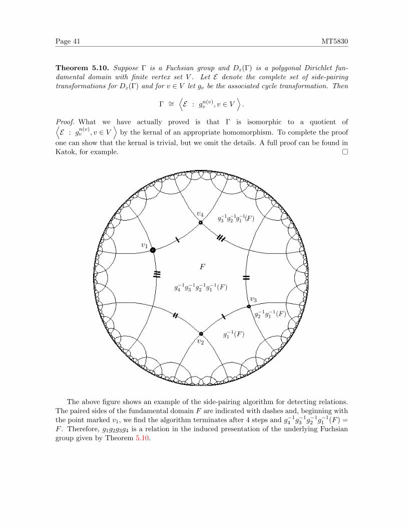
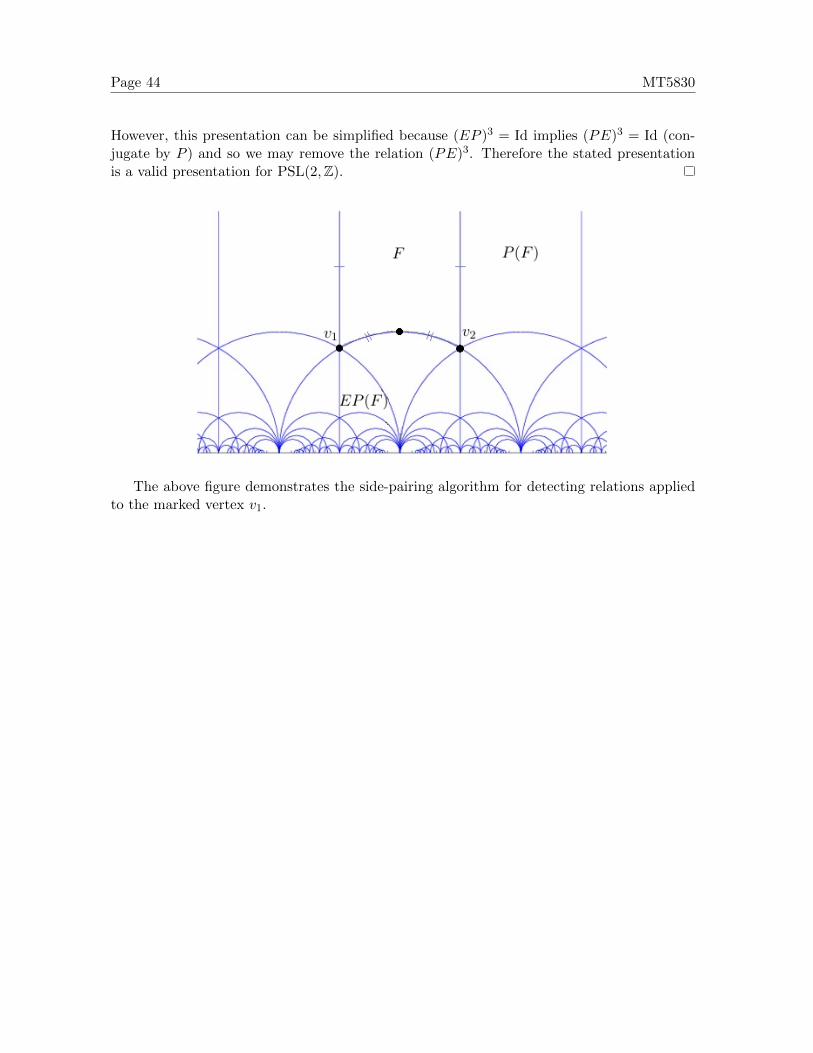
Elements of a Fuchsian group which take an edge of a fundamental domain to anotheredge are called called side-pairing transformations. The above lemma implies that the sides ofa polygonal Dirichlet fundamental domain come in pairs, which are mapped to each other by(unique) members of the Fuchsian group. There is one exception to this, which occurs if thereis an elliptic fixed point contained in one of the sides. In this case the elliptic transformationmaps this side to itself: fixing the fixed point and interchanging the segments either sideof it. Therefore, if we have such an elliptic fixed point, then we view it as a vertex of thefundamental domain and the elliptic transformation pairs the sides meeting at this vertex.With this convention, if Dz(Γ) is a polygonal Dirichlet fundamental domain then the sidescome in pairs which are mapped onto each other by the side-pairing transformations. Thismeans that the number of sides is always even!
Theorem 5.9. The collection of all the side-pairing transformations of a Dirichlet funda-mental domain for a Fuchsian group Γ are a generating set for Γ.
Proof. Let D be a Dirichlet fundamental domain for Γ, and let H be the group generatedby the side-pairing transformations. Clearly H 6 Γ and so the aim is to show that Γ ⊆ H.First note that if h ∈ H and g ∈ Γ are such that h(D) and g(D) are adjacent (i.e. have oneedge in common), then necessarily g ∈ H. This follows since h−1h(D) = D and h−1g(D)are adjacent, which implies that h−1g is a side-pairing transformation, and hence h−1g ∈ H.Then using the fact that H is a group we know g = hh−1g ∈ H as required.
Now, let g ∈ Γ be given with the aim to show that g ∈ H. In fact the above observationalready does the job via an inductive argument. Since Γ(D) is a ‘tiling’ of the hyperbolicplane, we can find a ‘chain’ of images g1(D), g2(D), . . . , gn(D) where g1 = Id, gn = g, andgk(D) is adjacent to gk+1(D) for k ∈ {1, . . . , n − 1}. Therefore for each such k, we havegk ∈ H ⇒ gk+1 ∈ H, and the desired result follows by induction.
The above theorem shows that the sides of a polygonal Dirichlet fundamental domainare in one-to-one correspondence with a set of generators for the Fuchsian group. It turnsout that the vertices of the fundamental domain are in one-to-one correspondence with therelations in a given presentation for the group.
We briefly recall the notion of a presentation. Given a finite set A and a finite set B ⊂ FAwhere FA is the free group over A, then we write
H ∼= 〈A : B〉
to mean the group generated by the elements of A, subject to the constraints that b = Idfor all b ∈ B. This way of expressing a group is known as a presentation and since A,B arefinite we say H is finitely presented. Elements of A are called generators and elements ofB are called relations. We will not worry about the details of presentations here but, moreformally,
〈A : B〉 ∼= FA/⟨BFA
⟩where BFA is the conjugation of B by FA, i.e.
BFA = {g−1hg : g ∈ FA, h ∈ B}.
This generates a normal subgroup⟨BFA
⟩E FA known as the normal closure of B in FA.
Thus the presentation 〈A : B〉 is formally the quotient of the free group over A by the normalclosure of B. Examples include, free groups
FA ∼= 〈A : ∅〉 ,
Page 40 MT5830
cyclic groups of order nCn ∼= 〈a : an〉 ,
and the integer lattice (or free abelian group of order 2)
Z× Z ∼=⟨a, b : a−1b−1ab
⟩.
Let E denote the finite set of edges and V the finite set of vertices of a polygonal Dirichletfundamental domain. For each v ∈ V ∩H2 we associate a relation as follows:
Step 1. Let v1 = v ∈ V , eg1 ∈ E be one of the edges adjacent to v1, and α1(v) be the angle atv1. Therefore g−1
1 eg1 = eg−11∈ E and g−1
1 (v1) ∈ V is a vertex adjacent to eg−11
.
Step 2. Let v2 = g−11 (v1), and α2(v) be the angle at v2. Since the domain is polygonal, there is
a unique edge eg2 ∈ E different from eg−11
adjacent to v2. Therefore g−12 eg2 = eg−1
2∈ E
and g−12 (v2) ∈ V is a vertex adjacent to eg−1
2.
Step 3. Let v3 = g−12 (v2) = g−1
2 (g−11 (v1)), and α3(v) be the angle at v3. Since the domain is
polygonal, there is a unique edge eg3 ∈ E different from eg−12
adjacent to v3. Therefore
g−13 eg3 = eg−1
3∈ E and g−1
3 (v3) ∈ V is a vertex adjacent to eg−13
.
...
Step k(v). Since V is finite, this process must return to v = v1 in a finite number k(v) of steps.This does not quite follow directly from finiteness (this just gives that we eventuallymust reach a vertex we have seen before), but the only vertex one can possibly visittwice is v1. This is because every vertex is adjacent to two sides and therefore has twopaths to it via this process. Once a vertex has been visited, both of these paths havebeen used (one ‘in’ and one ‘out’) and since we only went ‘out’ of v1, we must eventuallygo back ‘in’ to it.
Once we have returned to v1 we terminate the algorithm and conclude that
v = g−1k(v)(g
−1k(v)−1(· · · g−1
2 (g−11 (v)) · · · )).
This means that the cycle transformation at v given by g1 · · · gk(v) fixes v ∈ H2 and so iseither equal to the identity, or is an elliptic element with finite order n(v), i.e. for some(minimal) integer n(v) > 1 we have
(g1 · · · gk(v))n(v) = Id.
Note that an elliptic element of a Fuchsian group must have finite order, or it would violatethe fact that the group acts properly discontinuously.
If the cycle transformation is elliptic, then the orbit of the Dirichlet fundamental domainunder the the action of this map tiles a neighbourhood of v and this implies that v satisfiesthe angle sum condition:
n(v)
k(v)∑i=1
αi(v) = 2π.
We have almost proved the following theorem.
Page 41 MT5830
Theorem 5.10. Suppose Γ is a Fuchsian group and Dz(Γ) is a polygonal Dirichlet fun-damental domain with finite vertex set V . Let E denote the complete set of side-pairingtransformations for Dz(Γ) and for v ∈ V let gv be the associated cycle transformation. Then
Γ ∼=⟨E : gn(v)
v , v ∈ V⟩.
Proof. What we have actually proved is that Γ is isomorphic to a quotient of⟨E : g
n(v)v , v ∈ V
⟩by the kernal of an appropriate homomorphism. To complete the proof
one can show that the kernal is trivial, but we omit the details. A full proof can be found inKatok, for example.
The above figure shows an example of the side-pairing algorithm for detecting relations.The paired sides of the fundamental domain F are indicated with dashes and, beginning withthe point marked v1, we find the algorithm terminates after 4 steps and g−1
4 g−13 g−1
2 g−11 (F ) =
F . Therefore, g1g2g3g4 is a relation in the induced presentation of the underlying Fuchsiangroup given by Theorem 5.10.
Page 42 MT5830
5.2 Poincare’s Theorem
The last result in the previous section allows us to take a group, move to a fundamentaldomain, and then recover the group from the geometry of the fundamental domain via apresentation. In this mini-section, we state a remarkable converse. It says that, given a sen-sible polygon (satisfying the angle sum condition at each vertex for a given set of side-pairingtransformations), then one can obtain a Fuchsian group with this polygon as a fundamentaldomain.
If there are multiple vertices on the boundary of hyperbolic space, then there is anothertechnical condition to worry about. In particular, imagine that v a boundary vertex. Wecan associate a cycle transformation with v using the same algorithm as before. Side-pairingtransformations map boundary vertices to other boundary vertices and so if there is only oneboundary vertex then the associated cycle transformation is either one of the side-pairingtransformations associated to sides adjacent to v (these are mutually inverse). If there aremultiple boundary vertices, then the situation is more complicated.
Theorem 5.11 (Poincare’s Theorem). Let P be a hyperbolic polygon and let E be a completeset of side-pairing transformations for P . Assume that every vertex satisfies the angle sumcondition, i.e. for any vertex v of P , we have
n(v)
k(v)∑i=1
αi(v) = 2π
and that all cycle transformations associated with boundary vertices are either parabolic orthe identity (i.e., not hyperbolic). Then the group generated by E is a Fuchsian group with Pas a fundamental domain.
5.3 The modular group: fundamental domain, generators, and presenta-tions
There does not seem to be a simple general method for computing the Dirichlet fundamentaldomain for a given Fuchsian group. A good strategy is to think of a generating set whichcorresponds to the side-pairing transformations of a convex polygon and then prove directlythat this convex polygon is a Dirichlet region. As an example, we compute the Dirichletfundamental domain for the modular group Γ = PSL(2,Z). Let
F ={w ∈ H2 : −1/2 < Re(w) < 1/2 and |z| > 1
}.
We will prove that F is the Dirichlet region with base point z = 2i, i.e. F = D2i(Γ).First observe that 2i is not an elliptic fixed point of Γ. Indeed, recalling when we classifiedisometries by fixed points, the only way for 2i to be a fixed point of an element of PSL(2,R)was to choose a = d and b = −4c 6= 0 which violates ad − bc = a2 + 4c2 = 1 since c isa non-zero integer. The parabolic map z 7→ z + 1 is a side-pairing transformation for thevertical sides of F and the elliptic transformation z 7→ −1/z fixes i, splits the final side at iand pairs these sides. In particular, F ⊇ D2i(Γ).
Page 43 MT5830
We prove the reverse inclusion by contradiction. Suppose D2i(Γ) is a strict subset of F ,which guarantees the existence of w ∈ F and g ∈ Γ such that g(w) ∈ F . This follows sinceΓ(D2i(Γ)) tiles H2. Suppose g is defined by
g(w) =aw + b
cw + d
for a, b, c, d ∈ Z with ad − bc = 1. First note that c 6= 0, since if c = 0, then g(w) = w + band since b is an integer we cannot have both w and g(w) inside F . It follows that
(in the final line we use that c 6= 0 and c and d are integers). It follows that |cw + d|2 > 1and hence
Im(g(w)) = Im
((aw + b)(cw + d)
|cw + d|2
)=
Im(w)(ad− bc)|cw + d|2
=Im(w)
|cw + d|2< Im(w).
Arguing similarly with w and g replaced by g(w) and g−1 we obtain
Im(w) = Im(g−1(g(w))) < Im(g(w)),
which is a contradiction as required. We obtain the following group theoretic corollary byapplying Theorem 5.10.
Corollary 5.12. The modular group PSL(2,Z) is generated by the parabolic map P : z 7→ z+1and the elliptic map E : z 7→ −1/z and, moreover, has the following presentation
PSL(2,Z) ∼=⟨P,E : E2, (EP )3
⟩.
Proof. Since F is a Dirichlet fundamental domain it is generated by its side-pairing trans-formations {E,P, P−1} (and we may clearly drop P−1 from the generating set). Moreover,applying the side-pairing algorithm to the vertex i we find E2 = Id and so E2 is a relation.Applying the algorithm the other vertices in H2 we find E ◦ P = EP is an elliptic trans-formation of order 3 and PE is another elliptic transformation of order 3. This means that(EP )3 and (PE)3 are relations and we conclude
PSL(2,Z) ∼=⟨P,E : E2, (EP )3, (PE)3
⟩.
Page 44 MT5830
However, this presentation can be simplified because (EP )3 = Id implies (PE)3 = Id (con-jugate by P ) and so we may remove the relation (PE)3. Therefore the stated presentationis a valid presentation for PSL(2,Z).
The above figure demonstrates the side-pairing algorithm for detecting relations appliedto the marked vertex v1.
Page 45 MT5830
6 Fuchsian limit sets
The defining feature of a Fuchsian group is that it acts discontinuously on hyperbolic space.However, a Fuchsian group (usually) acts continuously on part of the boundary! The precisesubset of the boundary where the action is continuous is known as the limit set. Fuchsianlimit sets are interesting in their own right and often have a complicated fractal structure,but they are also intrinsically linked with the algebraic and geometric properties of the groupand its action. It is more convenient to set up the theory for Fuchsian groups acting on D2,but of course one can pass between the models via the Cayley map as usual.
More precisely, the limit set of a Fuchsian group Γ 6 con+(1) is defined by
L(Γ) = Γ(0) \ Γ(0)
where the closure is taken in the Euclidean metric. In other words, the limit set is the set ofaccumulation points of the orbit of 0 under the action of the group. A more direct, but morelaborious, way to write the limit set is
L(Γ) = {z ∈ C \ Γ(0) : there exists a sequence gn ∈ Γ such that |gn(0)− z| → 0}.
In this section we study Fuchsian limit sets L(Γ) in detail and begin by making some simplestructural observations.
Theorem 6.1. Fuchsian limit sets are closed subsets of the boundary of hyperbolic space, i.e.if Γ 6 con+(1) is a Fuchsian group, then
1. L(Γ) ⊆ S1
2. L(Γ) is closed in the Euclidean metric.
Proof. 1. follows immediately since Γ(0) is a discrete subset of D2. In particular, Γ(0)cannot accumulate anywhere except on the boundary. We will now prove 2. by proving thatif zn ∈ L(Γ) is a sequence of points such that zn → z, then z ∈ L(Γ). For each n, let gn,m ∈ Γbe such that gn,m(0)→ zn in the Euclidean metric as m→∞. We can find such gn,m sincezn ∈ L(Γ). We may also assume that gn,m(0) converges ‘uniformly quickly’ to zn by takingappropriate subsequences. More precisely, for a given n choose mn sufficiently large to ensurethat
At this point it seems that the limit set may depend on the choice of ‘base point’. Thebase point above is 0, but we could have defined the limit set to be the accumulation pointsof any w ∈ D2. It turns out that the limit set is independent of the base point and, moreover,the same sequence of maps will give rise to the same point in the limit set, independent ofthe base point.
Theorem 6.2. Fuchsian limit sets are independent of the choice of base point, i.e. if Γ 6con+(1) is a Fuchsian group and w ∈ D2, then
L(Γ) = Γ(w) \ Γ(w).
Page 46 MT5830
Proof. Let z ∈ L(Γ) and let gn ∈ Γ be such that gn(0)→ z. We will prove that gn(w)→ z foran arbitrary point w ∈ D2, which proves that L(Γ) ⊆ Γ(w) \ Γ(w) as required. The oppositeinclusion follows via a similar argument which we omit. Using con+(1) invariance and one ofthe standard formulae for the distance between two points we know that
Since gn(0)→ z ∈ S1 we know (1− |gn(0)|2)→ 0. This forces |gn(w)− gn(0)| → 0 as n→∞as otherwise the left hand side of the above equation would blow up. Therefore
|gn(w)− z| 6 |gn(w)− gn(0)|+ |gn(0)− z| → 0
as required.
A common theme in fractal geometry is to use the fact that the fractal may be a ‘dy-namical invariant’. For example, the middle third Cantor set is invariant under the mapx 7→ 3x (mod 1). One can then appeal to dynamical systems theory to study the fractal.Limit sets are invariant under the action of the associated Fuchsian group, and this propertyis often used to study the limit sets and the invariant measures they support.
Theorem 6.3. Limit sets are (strongly) invariant under the action of the associated Fuchsiangroup, i.e. if Γ 6 con+(1) is a Fuchsian group, then for all g ∈ Γ we have
g(L(Γ)) = L(Γ).
Proof. Let z ∈ L(Γ), g ∈ Γ, and let gn ∈ Γ be such that gn(0) → z. Since g is a continuousmap on the Euclidean disk, it follows that
g(gn(0))→ g(z)
which implies g(z) ∈ L(Γ). Thus we have proved that g(L(Γ)) ⊆ L(Γ). The opposite inclusionfollows by replacing g with g−1 and applying g.
After establishing Γ-invariance of the limit set, it should not come as a surprise that thelimit set contains all the hyperbolic and parabolic fixed points of elements of Γ. Of course,it cannot contain the elliptic fixed points because they lie in the interior of the disk.
Theorem 6.4. Limit sets contain all hyperbolic and parabolic fixed points, i.e. if Γ 6 con+(1)is a Fuchsian group and z ∈ S1 is fixed by some g ∈ Γ, then z ∈ L(Γ).
Proof. This follows immediately since if p ∈ S1 is fixed by a parabolic map g ∈ Γ, thengn(0)→ p and if h1, h2 ∈ S1 are the repelling and attracting fixed points of a hyperbolic mapg ∈ Γ, then
gn(0)→ h2 and g−n(0)→ h1.
The precise calculation is in the tutorial sheets.
Limit sets can be very complicated metric objects, but from a topological point of viewthere are only 5 possibilities. More precisely, only 5 different topological spaces can arise aslimit sets of Fuchsian groups. The most interesting of these is the ‘Cantor space’. A subsetof a metric space is a topological Cantor space if it is compact, totally disconnected, and
Page 47 MT5830
perfect. Recall that a subset of a metric space is totally disconnected if the only connectedsubsets are singletons. In particular, a subset of S1 is totally disconnected if and only ifgiven any two points in the set there is a point not in the set on both the clockwise and anti-clockwise arcs between the two given points. A subset of a metric space is perfect if everypoint is an accumulation point. An important result in topology is that being compact,totally disconnected, and perfect uniquely defines a topological space up to homeomorphism.
Theorem 6.5. Let Γ 6 con+(1) be a Fuchsian group. Then
1. L(Γ) = ∅ if and only if Γ consists only of elliptic elements,
2. |L(Γ)| = 1 if and only if Γ is generated by a single parabolic element,
3. |L(Γ)| = 2 if and only if Γ is generated by a single hyperbolic element, or if it is generatedby a single hyperbolic element and a collection of elliptic involutions (elements of order2) which interchange the hyperbolic fixed points.
4. in all other cases L(Γ) is either equal to S1 or is a topological Cantor space. In partic-ular, L(Γ) is a continuum (has the same cardinality as R).
Proof. If L(Γ) = ∅, then Γ has no fixed points on the boundary and therefore must consistonly of elliptic elements.
If |L(Γ)| = 1, then there are no hyperbolic elements since they have 2 fixed points.Also there must be at least one parabolic element and all parabolic elements must fix thesame point. Since Γ is discrete, this guarantees that all parabolic elements are powers of acommon parabolic element. Finally, there are no elliptic elements because a singleton cannotbe invariant under a non-trivial rotation.
If |L(Γ)| = 2, then there cannot be any parabolic elements since they fix precisely onepoint. If there are no elliptic elements, then every element must fix the two points in thelimit set and again using discreteness must all be powers of the same hyperbolic element.Moreover, elliptic elements which do exist must interchange the two fixed points and are thusinvolutions.
Let Γ be a Fuchsian group whose limit set has at least 3 points. Fix any three distinctpoints z1, z2, z3 ∈ L(Γ) and let w ∈ D2 be any point on the geodesic ray joining z2 andz3. Our aim is to show that z1 is an accumulation point in L(Γ). Let gn ∈ Γ be distinctelements such that gn(w) → z1 (recall the limit set is independent of the base point). Takea subsequence of the gn such that gn(z2) and gn(z3) both converge in the Euclidean metricto (not necessarily distinct) points z2, z3 ∈ S1 respectively (we can do this by compactness).This implies that gn(w) converges in the Euclidean metric to a point on the geodesic rayjoining z2 and z3. However, since we already know gn(w) → z1 we may conclude that atleast one of z2 and z3 is equal to z1. We assume without loss of generality that z2 = z1. Ifat most finitely many n satisfy gn(z2) = z1, then we can conclude that z1 is an accumulationpoint. This follows since Γ(z2) ⊆ L(Γ) by Γ-invariance. Therefore, we assume withoutloss of generality that gn(z2) = z1 for all n. Since elements of con+(1) are determined bytheir action on two points, it follows that the points gn(z3) are all distinct and thereforez3 is an accumulation point in L(Γ). If z3 = z1, then again we can conclude that z1 is anaccumulation point and so we further assume that z3 6= z1. The strategy now is to drag z3
towards z1. Consider the (distinct) points z3 and g−11 (z3). We know gn(z3) → z3 6= z1 and
so gn(g−11 (z3))→ z1 by repeating the above argument. Since z3 is an accumulation point, we
Page 48 MT5830
know g−11 (z3) is an accumulation point and so z1 is the limit of accumulation points and so
is itself an accumulation point. Since z1 was arbitrary we conclude that L(Γ) is perfect.We already know that L(Γ) is closed and bounded, and thus compact, and so it remains
to show that if L(Γ) has at least three points and L(Γ) 6= S1, then it is totally disconnected.Let z1, z2 ∈ L(Γ) be distinct points and suppose u ∈ S1 \ L(Γ). It suffices to show thatthere is a point in the clockwise arc from z1 to z2 which is not in L(Γ). The anti-clockwisearc can be dealt with similarly. Since L(Γ) is closed, we can find an open neighbourhoodof u which is disjoint from L(Γ). Let u1, u2 be the end points of this open neighbourhood(which is an open arc in S1). Let t ∈ S1 be an arbitrary point in the clockwise arc from z1
to z2. If t /∈ L(Γ), then we are done and so we can assume t ∈ L(Γ). Arguing as above wecan find a sequence of maps gn ∈ Γ such that either gn(u1) or gn(u2) converges to t in theEuclidean metric. Using strong Γ-invariance again this guarantees the existence of a point inthe clockwise arc from z1 to z2 which is not in L(Γ).
We say a Fuchsian group is an elementary Fuchsian group if it has a finite limit set (i.e.we are in one of the first three cases in the above theorem). Otherwise it is called a non-elementary Fuchsian group. Note that in both the second and third cases (when there are noelliptic elements, Γ ∼= (Z,+), the infinite cyclic group. This is a simple demonstration thatthe limit set is not a purely group theoretic concept (invariant under group isomorphism).
The above figure depicts a subgroup of con(1) generated by reflection in three geodesicrays. Groups generated in this way are called (hyperbolic) reflection groups. The orbit of0 is shown in red and the fundamental domain is labelled F . Note that reflection groupsare strictly speaking not Fuchsian because reflections are orientation reversing. However, theorientation preserving elements of a reflection group form a Fuchsian subgroup of index 2and the limit set is the same for both groups.
Page 49 MT5830
6.1 The Poincare series and dimension of the limit set
The Poincare series of a Fuchsian group Γ 6 con+(1) measures how quickly the orbit Γ(0)accumulates on the boundary. Heuristically, the faster the accumulation, the smaller thelimit set is. More formally, we define a function P : [0,∞)→ [0,∞] by
PΓ(s) =∑g∈Γ
e−sdD2 (0,g(0)) =∑z∈Γ(0)
e−sdD2 (0,z) =∑z∈Γ(0)
(1− |z|1 + |z|
)sand refer to PΓ(s) as the Poincare series of Γ with exponent s > 0. The faster the orbit Γ(z)accumulates at the boundary, the smaller P (s) is and in order to quantify this precisely, theexponent of convergence of Γ is defined by
δ(Γ) = inf{s > 0 : PΓ(s) <∞}.
The most standard way to quantify the ‘size’ of a fractal set is by its ‘dimension’. TheHausdorff dimension is defined for any subset of a metric space and generalises our intuitiveconception of the dimension of smooth objects to fractals. For example, the Hausdorff dimen-sion of any countable set is 0, the Hausdorff dimension of S1 is 1, the Hausdorff dimensionof the Euclidean plane C is 2, but the Hausdorff dimension of the (non-smooth) middle thirdCantor set is log 2/ log 3 ≈ 0.6309 . . . . Unfortunately, the precise definition and study of theHausdorff dimension is beyond the scope of this course, but we end with a beautiful (andcomparatively recent) result concerning the challenging question of computing the dimensionof a Fuchsian limit set. We write dimHE to denote the Hausdorff dimension of a set E.
Theorem 6.6. If Γ is a finitely generated non-elementary Fuchsian group, then
dimH L(Γ) = δ(Γ).
6.2 Non-examinable
This important theorem dates back to an influential paper of Samuel J. Patterson from1976 (Acta Mathematica). Patterson received his PhD from Cambridge in 1975 under thesupervision of Alan Beardon (author of one of the main references for this course) and hasworked in Gottingen since 1981. It was here that he supervised the PhD of Bernd Stratmann,who later joined the University of St Andrews and taught me hyperbolic geometry in 2009!
This theorem holds for certain classes of infinitely generated Fuchsian groups, includinggeometrically finite groups. Roughly speaking a Fuchsian group is geometrically finite if ithas a ‘reasonable’ fundamental domain. The result was generalised to higher dimensional hy-perbolic spaces (where the analogous groups are called Kleinian groups) by Dennis Sullivanin 1979. Those familiar with fractal geometry and dimension theory will know that there areseveral other notions of dimension apart from the Hausdorff dimension. In 1996 Stratmannand Urbanski proved that the upper and lower box-counting dimensions and packing dimen-sion of the limit set of a geometrically finite non-elementary Kleinian group is also equalto the exponent of convergence (and thus coincide with the Hausdorff dimension). Anotherpopular notion of dimension is the Assouad dimension, which behaves rather differently inthis setting. I proved that the Assouad dimension of the limit set of a geometrically finitenon-elementary Kleinian group is equal to the maximum of the exponent of convergence andthe maximal rank of a free abelian subgroup of the stabiliser of a parabolic point. This sounds
Page 50 MT5830
more complicated than it is and in the 2-dimensional setting of this course, this simplifies to:if there are no parabolic elements, then the Assouad dimension is the exponent of conver-gence, and, if there is a parabolic element, then the Assouad dimension of the limit set is 1(the maximal value possible).
The above figure shows three limit sets of Kleinian groups acting on three dimensionalhyperbolic space. The one on the left is a discrete subgroup of con+(2) which acts on D3
(the three dimensional disk). The boundary of this space is S2 and the limit set is a fractalsubset of the boundary. The other two images are subsets of C, which is the boundary ofthree dimensional hyperbolic space when modelled by
H3 = R+ × C
(the three dimensional analogue of the upper half-plane model). The group of (orientationpreserving) isometries in this case is PSL(2,C). The image in the middle is more commonlyrecognised as an Apollonian circle packing, constructed as follows: begin with four mutu-ally tangent circles, one of which contains the other three. Now draw the biggest circle youcan inside the large initial circle, whose interior does not overlap the interiors of the threecircles initially inside the large one. This circle will necessarily be tangent to three of thefour initial circles. Continue in this way ad infinitum and the set of all the boundaries ofcircles you have added (including the initial four) is the Apollonian circle packing. Althoughthe precise packing you obtain depends on the location of the initial four circles, it turnsout that any Apollonian packing can be mapped onto any other via a Mobius map (re-call that circles are mapped to circles). See Mark Pollicott’s expository paper, found herehttp://homepages.warwick.ac.uk/~masdbl/apollo-29Dec2014.pdf, for more details onthe history and persistent mathematical interest in Apollonian circle packings.