Multi-Asset Investments and Portfolio Solutions Blind ......Blind faith: Do target date funds miss...

March 2016

Multi-Asset Investments and Portfolio Solutions

by Fred Dopfel, PhD, Senior Adviser

Blind faith: Do target date funds miss the mark by relying on age-based allocation?

For Financial Intermediary, Institutional and Consultant use only.Not for redistribution under any circumstances.

M U L T I - A S S E T I N V E S T M E N T S & P O R T F O L I O S O L U T I O N S

2

Target date funds have ridden a wave of success in asset growth and popularity

among defi ned contribution plans.1 This may be due to perception rather than

proven performance—a perception of risk protection provided by the glide path

approach that reduces investment risk as participants get closer to retirement.

But this expected risk protection failed during recent fi nancial market swings,

as most funds were “blind” to market conditions and participants suffered large

losses as a result. An important lesson over the past two decades has been that

target date funds (and balanced funds) are subject to signifi cant drawdown risk

that hurts participants’ chances of successful retirement outcomes.

This paper asks two essential questions:

1. Should asset allocation strategies be based solely on the age of the

participant (time to retirement), or should they be adjusted continually,

to take advantage of market opportunities and protect from

market threats?

2. If asset allocation is adjusted according to market conditions, how

much “investment skill” does a manager need in order to provide better

performance for the strategy and better retirement outcomes

for participants?

Introduction


3

We approach these two essential questions by fi rst describing the types of asset

allocation strategies examined and defi ning our participant assumptions. From

these assumptions, we compare performance of a glide path strategy (which

changes asset allocation based on the time to retirement) with that of a static

balanced strategy (which maintains the same allocation). Next, we describe a

dynamic strategy, such as risk-controlled growth, which adjusts asset allocation

based on market opportunities. We then calculate the performance of this

dynamic strategy versus a balanced strategy, by varying the manager’s level

of investment skill. Finally, we look at the potential improvement in retirement

outcomes for each option. In the end, we seek to identify which strategies are

most likely to yield better retirement outcomes for participants—glide path or

balanced, dynamic or static.

We fi nd that asset allocation strategies based on age alone have relatively little

impact on retirement outcomes, despite public opinion to the contrary. Asset

allocation based on market conditions can potentially have much larger effects

on retirement outcomes, even if the manager chosen has only a moderate

degree of investment skill.


4

Two dimensions of asset allocation strategies are depicted in Exhibit 1. The vertical dimension is balanced versus glide path, which addresses whether or not asset allocation changes according to the participant’s age or time to retirement. The horizontal dimension is static versus dynamic, which addresses whether or not asset allocation changes according to market opportunities and threats.

Balanced refers to asset allocation strategies that are set without regard to age or time to retirement. In contrast, a glide path strategy has an asset allocation that is mechanically adjusted to become more conservative as the retirement date approaches.

Exhibit 1: Dimensions of asset allocation strategies

Static, as opposed to dynamic, here refers to strategies that have a pre-assigned asset allocation that does not change with market conditions. For example, a standard 60/40 stock/bond portfolio is a static balanced strategy. An example of a static glide path strategy is a traditional target date fund.

Dynamic strategies refer to asset allocations that are adjusted based on market opportunities and risks, as in a risk-controlled growth (RCG) strategy.2 Properly evaluating market opportunities and risks requires a minimum threshold of investment skill in order to identify economic regimes, business cycles, and anomalies in valuation. In the presence of suffi cient skill, we would expect dynamic strategies such as these to outperform static strategies. Risk-controlled growth is an example of a dynamic balanced strategy; other tactical asset allocation (TAA) strategies may also fi t this category. An RCG strategy, or other TAA strategy, could also be set up as an overlay on a glide path investment policy. This latter example is called a dynamic glide path strategy. Strategies can be any combination on these two dimensions—a dynamic or a static approach could be centered upon either a balanced or glide path policy.

Investment dimensions and participant assumptions

1

Source: Schroders. For illustration only.

Glide Pathasset allocation

depends on age or time to retirement

Balancedasset allocation

does not depend on age or time to retirement

Staticasset allocation

does not adjust based on market opportunities

Dynamicasset allocation

adjusts based on market opportunities

Traditional Target Date

Fund

RCG Overlay on

Target Date Fund

Balanced60/40

Portfolio

Risk-Controlled

Growth(RCG)


5

Desired retirement outcomesDefi ned contribution participants invest wages during their working years for the purpose of future spending needs during retirement. Thus, our attention should focus primarily on the goal of improving the likelihood of attaining successful retirement outcomes as measured by the replacement of pre-retirement income. A simple and well-accepted way to measure retirement outcomes is with the replacement ratio (RR), indicating how much income is needed to continue one’s lifestyle during retirement:

Replacement ratio = income during retirement / pre-retirement income

Full replacement of income during the retirement years, or RR = 100%, is likely unnecessary, because there is usually lower saving, lower income taxes, and lower spending during the golden years. A gross replacement ratio of approximately 75% is a reasonable and commonly used target to continue one’s lifestyle during retirement, although the optimal target varies according to income level and other factors. An individual’s income from other sources, such as Social Security, amounts to about 25% of pre-retirement income, on average.3 This means that individuals, on average, should set a goal of a net replacement ratio of 50% from the DC plan.

If a participant attains a net RR = 50% or greater from the DC plan, then we are in a reasonable range. But there may be a wide variation in realized replacement ratios; to protect against the downside, we should consider less fortunate circumstances. For instance, realizing a net RR of only 35% (gross RR = 60%) would lower one’s lifestyle materially, but would likely not leave a person in a ruinous situation. We assume that a participant would like to limit the possibility of this event to a 1-in-10 chance or less.

The simple statement of desired outcomes from the DC plan is that we want to attain a median replacement ratio of 50% or better, and a lower-decile RR of 35% or better. An upper-decile RR of 100% or better is attractive, but the main concern is the expected outcome and the downside scenarios. We will focus on the full working life, beginning at age 25 with 40 years to retirement, but we are also interested in the shorter horizon faced by a 55 year old with only 10 years to retirement.

Describing our model participant and investment opportunitiesIndividual participants vary a great deal, so we need to make some modelling assumptions. We assume that our model participant has a successful career, has steady growth in income, is long-lived with a 40-year work life, and is disciplined about long-term savings through the DC plan, beginning with a 10% contribution rate (including employer match).4 This description signifi es exemplary behavior by the participant. Our choice of the model participant is intentional, in order to provide a higher likelihood of realizing successful retirement outcomes, which we will indeed fi nd challenging to attain for participants that are less diligent about savings.

Our simulations use a “bootstrap” procedure, which is designed to provide a large number of possible scenarios for participants from historical market data. Instead of a theoretical distribution of returns based on forward-looking assumptions, we sample from actual experience over 87 years of fi nancial history.5 See endnote 5 for further detail regarding the assumptions underlying the simulations and the limitations inherent in any performance simulation. This method generates a distribution of portfolio returns that includes unexpected and rare events, which might otherwise be less represented by the standard normal distribution assumptions that are used in Monte Carlo approaches. These random samples from history may be more or less favorable than what we will experience over the next several decades. But the crucial factor to our analysis is the variability of returns rather than the level of returns, as we will evaluate the success or failure of various strategies in attaining retirement outcomes on a relative rather than an absolute basis.


6

The favored approach to defi ned contribution asset allocation over the last decade or more has been target date funds, which use a glide path approach. They are the most common qualifi ed default investment alternative (QDIA) offered by DC plans, and represent over $650 billion in mutual fund assets in the US, as of 2014.6 These funds, by defi nition, are intended to reduce total portfolio risk as the individual approaches retirement, via a decreasing allocation to equities on a predetermined basis.

As one example, although there is a tremendous variety of cases, consider a simplifi ed glide path strategy that begins with an allocation of 90% to equities (10% to bonds) at age 25, and brings the allocation down evenly each year to 30% equities (70% bonds) at age 65. The average allocation to equities in this example is 60% over the 40 years of a working life. To evaluate the effi cacy of the glide path approach, we compare its performance with a balanced 60% equities / 40% bonds allocation. Note that, while glide path formulae vary, this is a fair comparison, as the average exposure to equities is the same for glide path as for balanced in this set-up. No investment skill is required in either case, but how does performance compare?

Both policies fall a bit short of our desired outcomes for our model participant with a 40-year working life, as shown in Exhibit 2. A balanced 60/40 policy nearly attains the desired median replacement ratio, with a median RR = 49%. Glide path results are less favorable, with median RR = 45%. The lower-decile results fall short of our desired outcomes in both cases (downside RR = 29% and 28%). Based on this analysis alone, the participant’s choice is likely to be in favor of a balanced policy, given a +4% gain in median RR against only a 1% reduction in the 1-in-10 downside RR.

Exhibit 2: Glide path vs. balanced - replacement ratio comparison at age 25

Performance of glide path versus balanced

2

Source: Schroders. See the Appendix for asset class return data.

htaP edilG citatSdecnalaB citatS

Upper Decile %47%58

Lower Decile %92%82

Median %54%94

0%10%20%30%40%50%60%70%80%90%

100%

Repla

ceme

nt Ra

tio

Goal for median RR

Goal for downside RR


7

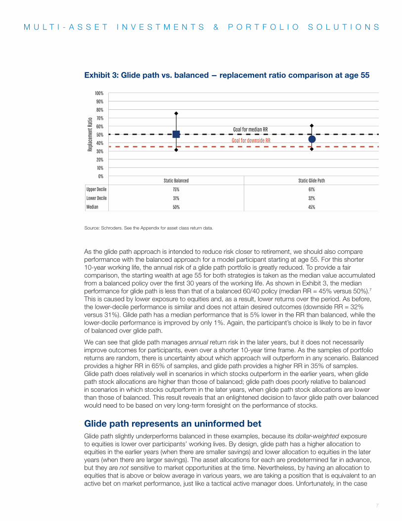
Exhibit 3: Glide path vs. balanced - replacement ratio comparison at age 55

htaP edilG citatSdecnalaB citatS

Upper Decile %16%57

Lower Decile %23%13

Median %54%05

0%

10%

20%

30%

40%

50%

60%

70%

80%

90%

100%Re

place

ment

Ratio

Goal for median RR



As the glide path approach is intended to reduce risk closer to retirement, we should also compare performance with the balanced approach for a model participant starting at age 55. For this shorter 10-year working life, the annual risk of a glide path portfolio is greatly reduced. To provide a fair comparison, the starting wealth at age 55 for both strategies is taken as the median value accumulated from a balanced policy over the fi rst 30 years of the working life. As shown in Exhibit 3, the median performance for glide path is less than that of a balanced 60/40 policy (median RR = 45% versus 50%).7 This is caused by lower exposure to equities and, as a result, lower returns over the period. As before, the lower-decile performance is similar and does not attain desired outcomes (downside RR = 32% versus 31%). Glide path has a median performance that is 5% lower in the RR than balanced, while the lower-decile performance is improved by only 1%. Again, the participant’s choice is likely to be in favor of balanced over glide path.

We can see that glide path manages annual return risk in the later years, but it does not necessarily improve outcomes for participants, even over a shorter 10-year time frame. As the samples of portfolio returns are random, there is uncertainty about which approach will outperform in any scenario. Balanced provides a higher RR in 65% of samples, and glide path provides a higher RR in 35% of samples. Glide path does relatively well in scenarios in which stocks outperform in the earlier years, when glide path stock allocations are higher than those of balanced; glide path does poorly relative to balanced in scenarios in which stocks outperform in the later years, when glide path stock allocations are lower than those of balanced. This result reveals that an enlightened decision to favor glide path over balanced would need to be based on very long-term foresight on the performance of stocks.

Glide path represents an uninformed betGlide path slightly underperforms balanced in these examples, because its dollar-weighted exposure to equities is lower over participants’ working lives. By design, glide path has a higher allocation to equities in the earlier years (when there are smaller savings) and lower allocation to equities in the later years (when there are larger savings). The asset allocations for each are predetermined far in advance, but they are not sensitive to market opportunities at the time. Nevertheless, by having an allocation to equities that is above or below average in various years, we are taking a position that is equivalent to an active bet on market performance, just like a tactical active manager does. Unfortunately, in the case


8

of glide path, the positions are uninformed by market conditions or forecasts. There is no skill involved, and we will be lucky or unlucky, based on the chance that performance in the early years is (on average) better or worse than performance in the later years. There is no real risk control either; with a glide path or a balanced strategy, any large deviation in wealth in a single year—early or late in one’s working life—propagates forward to fi nal wealth.

Instead of making preprogrammed adjustments to asset allocation that are blind to market conditions (as with static glide path), we now consider the impact of making informed adjustments to asset allocation, presuming that we have some insight about market conditions. We explore dynamic asset allocation strategies, such as RCG, which promise an ability to adjust asset allocation to enhance expected return and reduce drawdowns, based on investment skill.

We do not expect that anyone would have suffi cient “market timing” skill to be successful in going “all in” or “all out” of the market based on a forecast. Instead, we consider the lesser claim that some highly skilled managers can be successful, sometimes, by making measured annual changes to the allocation to stocks and bonds based on observing anomalies in market pricing and other insights on macroeconomic conditions. These insights may be based on a research process including: relative valuation of equities, bonds, and other asset classes; market volatility measures; and market cycle analysis. A risk-controlled growth strategy would consider all of these elements as part of a more frequent rebalancing process.

A simplifi ed dynamic asset allocation strategyFor this paper, we need to drastically simplify our description of a dynamic strategy in order to reach some general conclusions about the impact of investment skill. Assume that we receive annual signals from our research that suggest the future performance of stocks versus bonds will be high (upper third), medium (middle third), or low (lower third). Based on the signal, we change our portfolio relative to the balanced 60/40 or glide path policy, as follows:

Buy: If “high” signal, increase equity holdings by 15%, decrease bond holdings by 15%.

Hold: If “medium” signal, maintain equity and bond holdings.

Sell: If “low” signal, decrease equity holdings by 15%, increase bond holdings by 15%.

The choice of ±15% annual adjustments is fairly arbitrary, but results in a level of risk that may be acceptable for the participant.8 The signal is “noisy,” refl ecting the limitations of our skill in projecting future returns, and we may frequently be wrong. A correct signal is when the “high” signal leads to the future realized high performance of stocks relative to bonds (upper third); in this case, we “buy” based on the signal and have a relatively good outcome over the following year. An incorrect signal is when the signal does not correspond to the future realized performance; in this case, we bought when we should have sold, or we sold when we should have held, and so on, resulting in a relatively poor outcome.

The probability of a correct choice, based on the agreement between the signal and the outcome, is denoted by “p.” The probability of an incorrect choice, (1 – p), is split equally between the other two options.9 This is an intuitive measure for investors to think about when assessing the investment skill imbedded in a dynamic strategy.

Performance of dynamic versus static3


9

Assuming high skill, we further assume the probability of a correct choice may be p = 2/3; that is, the forecast is correct two-thirds of the time. Assuming no skill whatsoever, we expect the probability of a correct choice to be p = 1/3. It is possible that some managers may be worse than “no skill” and be distinguished by possessing “negative skill,” or p < 1/3! However, we shall assume that successful managers that we select have “positive skill” that falls within the range of p = 1/3 to p = 2/3. An investor’s assessment of investment skill is highly subjective. How much does the manager’s investment skill matter?

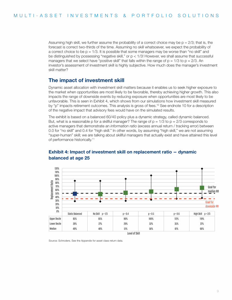
The impact of investment skillDynamic asset allocation with investment skill matters because it enables us to seek higher exposure to the market when opportunities are most likely to be favorable, thereby achieving higher growth. This also impacts the range of downside events by reducing exposure when opportunities are most likely to be unfavorable. This is seen in Exhibit 4, which shows from our simulations how investment skill measured by “p” impacts retirement outcomes. This analysis is gross of fees.10 See endnote 10 for a description of the negative impact that advisory fees would have on the simulated results.

The exhibit is based on a balanced 60/40 policy plus a dynamic strategy, called dynamic balanced. But, what is a reasonable p for a skillful manager? The range of p = 1/3 to p = 2/3 corresponds to active managers that demonstrate an information ratio (excess annual return / tracking error) between 0.0 for “no skill” and 0.4 for “high skill.” In other words, by assuming “high skill,” we are not assuming “super-human” skill; we are talking about skillful managers that actually exist and have attained this level of performance historically.11

Exhibit 4: Impact of investment skill on replacement ratio - dynamic balanced at age 25

Static Balanced No Skill p = 1/3 p = 0.4 p = 0.5 p = 0.6 High Sk

85% 85% 90% 100% 112% 119%

28% 27% 29% 32% 35% 37%

49% 48% 51% 56% 61% 66%

ill p = 2/3

Upper Decile

Lower Decile

Median

0%10%20%30%40%50%60%70%80%90%

100%110%120%

Repla

ceme

nt Ra

tio

Level of Skill

Goal for median RR




10

Summary of retirement outcomes for each option

4

Having assessed the impact of skill for a balanced strategy, and the relative performance of glide path versus balanced, next we evaluate other options. A dynamic strategy can also be combined with a glide path policy as a tactical overlay. Exhibit 5 lines up the outcomes for a static versus dynamic approach for balanced and glide path policies at age 25, with 40 working years until retirement. Here we have assumed a high level of skill (p = 2/3) to show the full potential impact of investment skill. Outcomes for a dynamic balanced strategy exceed desired levels; static balanced strategy outcomes fall short. Outcomes for a dynamic glide path strategy exceed desired levels also. Static glide path outcomes fall short.

Despite all the attention given to glide paths and their perceived benefi ts, we see that the largest impact on retirement outcomes is from skillful dynamic versus static asset allocation, rather than the choice of a glide path versus balanced asset allocation. As noted, low levels of skill produce modestly worse outcomes. But even at intermediate levels of skill, it appears that, outside of participant characteristics, the greatest impact on retirement outcomes is the impact of investment skill.

Exhibit 4 shows that there is a steady improvement in the median replacement ratio from 48% at no skill (p = 1/3) to 66% at high skill (p = 2/3). Our goal of a median replacement ratio of 50% or better is attained even with low skill (p between 1/3 and 0.4). The downside outcomes are also improved with skillful dynamic asset allocation. The lower-decile replacement ratio improves from 27% at no skill to 37% at high skill. Our goal of a lower-decile replacement ratio of 35% or better is attained only at high skill levels (p = 0.6 or better). The secondary goal for an upper-decile RR of 100% or better is attained at medium skill levels (p = 0.5 or better).

We should be concerned that we might select a dynamic strategy with presumed skill but, in fact, investment skill is absent. How damaging would this be for retirement outcomes? In the absence of any investment skill, we fi nd a small negative impact of the dynamic strategy, comparing the “no skill” results (p = 1/3) to the static balanced results. This defi ciency is caused by slightly higher risk resulting from annual changes to the asset allocation that do not provide a consistent extra return. The no-skill dynamic strategy reduces the median replacement ratio by 1% and lowers the downside RR by 1%. But moving up from “no skill” to “low skill” (p = 0.4), we fi nd a slight benefi t over the static strategy—a 2% improvement in the median RR and a 1% improvement in the downside RR. Low skill does not improve our outcomes materially, but it also does not hurt our chances of good outcomes severely.


11

Exhibit 5: Dynamic vs. static - outcomes for replacement ratio at age 25

Upper Decile %301%47%911%58

Lower Decile %73%92%73%82

Median %16%54%66%94

0%10%20%30%40%50%60%70%80%90%

100%110%120%

Repla

ceme

nt Ra

tio


Goal for median RR

Static Balanced Dynamic Glide PathStatic Glide PathDynamic Balanced


At age 55, with only 10 years to retirement, the story is similar, as shown in Exhibit 6.

Exhibit 6: Dynamic vs. static - outcomes for replacement ratio at age 55

Static Balanced

Upper Decile %86%16%38%57

Lower Decile %63%23%53%13

Median %05%54%55%05

0%10%20%30%40%50%60%70%80%90%

100%110%120%

Repla

ceme

nt Ra

tio

Goal for median RR


Dynamic Glide PathStatic Glide PathDynamic Balanced



12

ConclusionWhether a glide path or a balanced strategy will provide the best retirement outcome is very uncertain—especially looking out 40 years. The odds slightly favor a balanced approach over a glide path approach, but the eventual winning strategy depends on the unknowable future performance of stocks in the early years compared with the late years of one’s working life. Therefore, choosing glide path over balanced is likely to be an uninformed bet, at best. This observation points to the value of dynamic approaches that are “market aware” as a way of potentially improving retirement outcomes.

A risk-controlled growth strategy, or other dynamic approach, can be a part of either a glide path or a balanced asset allocation option. As glide path and balanced strategies often perform in a similar range, we have highlighted that based on our simulations, the most important choice for participants is for a dynamic approach over a static approach. A decision in favor of dynamic should be infl uenced by the availability of skillful dynamic asset allocation strategies, such as risk-controlled growth. The presence of superior investment skill must be validated by an evaluation of a strategy’s solid investment framework and historical track record.

The major conclusion of this paper is that a dynamic approach may perform better than a static glide path approach in managing both median and downside retirement outcomes. From the fi duciary perspective, the focus on downside performance is a very relevant consideration in making dynamic strategies available to defi ned contribution participants. We believe dynamic approaches such as risk-controlled growth ought then to be considered as very worthwhile additions to investment options that are currently available.


13

Appendix: Annual returns data (1928-2014)

Year Infl ation 3-month T. Bill

10-year T. Bond S&P 500

1928 -1.16% 3.08% 0.84% 43.81%

1929 0.58% 3.16% 4.20% -8.30%

1930 -6.40% 4.55% 4.54% -25.12%

1931 -9.32% 2.31% -2.56% -43.84%

1932 -10.27% 1.07% 8.79% -8.64%

1933 0.76% 0.96% 1.86% 49.98%

1934 1.52% 0.32% 7.96% -1.19%

1935 2.99% 0.18% 4.47% 46.74%

1936 1.45% 0.17% 5.02% 31.94%

1937 2.86% 0.30% 1.38% -35.34%

1938 -2.78% 0.08% 4.21% 29.28%

1939 0.00% 0.04% 4.41% -1.10%

1940 0.71% 0.03% 5.40% -10.67%

1941 9.93% 0.08% -2.02% -12.77%

1942 9.03% 0.34% 2.29% 19.17%

1943 2.96% 0.38% 2.49% 25.06%

1944 2.30% 0.38% 2.58% 19.03%

1945 2.25% 0.38% 3.80% 35.82%

1946 18.13% 0.38% 3.13% -8.43%

1947 8.84% 0.57% 0.92% 5.20%

1948 2.99% 1.02% 1.95% 5.70%

1949 -2.07% 1.10% 4.66% 18.30%

1950 5.93% 1.17% 0.43% 30.81%

1951 6.00% 1.48% -0.30% 23.68%

1952 0.75% 1.67% 2.27% 18.15%

1953 0.75% 1.89% 4.14% -1.21%

1954 -0.74% 0.96% 3.29% 52.56%

1955 0.37% 1.66% -1.34% 32.60%

1956 2.99% 2.56% -2.26% 7.44%

1957 2.90% 3.23% 6.80% -10.46%

1958 1.76% 1.78% -2.10% 43.72%



1959 1.73% 3.26% -2.65% 12.06%

1960 1.36% 3.05% 11.64% 0.34%

1961 0.67% 2.27% 2.06% 26.64%

1962 1.33% 2.78% 5.69% -8.81%

1963 1.64% 3.11% 1.68% 22.61%

1964 0.97% 3.51% 3.73% 16.42%

1965 1.92% 3.90% 0.72% 12.40%

1966 3.46% 4.84% 2.91% -9.97%

1967 3.04% 4.33% -1.58% 23.80%

1968 4.72% 5.26% 3.27% 10.81%

1969 6.20% 6.56% -5.01% -8.24%

1970 5.57% 6.69% 16.75% 3.56%

1971 3.27% 4.54% 9.79% 14.22%

1972 3.41% 3.95% 2.82% 18.76%

1973 8.71% 6.73% 3.66% -14.31%

1974 12.34% 7.78% 1.99% -25.90%

1975 6.94% 5.99% 3.61% 37.00%

1976 4.86% 4.97% 15.98% 23.83%

1977 6.70% 5.13% 1.29% -6.98%

1978 9.02% 6.93% -0.78% 6.51%

1979 13.29% 9.94% 0.67% 18.52%

1980 12.52% 11.22% -2.99% 31.74%

1981 8.92% 14.30% 8.20% -4.70%

1982 3.83% 11.01% 32.81% 20.42%

1983 3.79% 8.45% 3.20% 22.34%

1984 3.95% 9.61% 13.73% 6.15%

1985 3.80% 7.49% 25.71% 31.24%

1986 1.10% 6.04% 24.28% 18.49%

1987 4.43% 5.72% -4.96% 5.81%

1988 4.42% 6.45% 8.22% 16.54%

1989 4.65% 8.11% 17.69% 31.48%



1990 6.11% 7.55% 6.24% -3.06%

1991 3.06% 5.61% 15.00% 30.23%

1992 2.90% 3.41% 9.36% 7.49%

1993 2.75% 2.98% 14.21% 9.97%

1994 2.67% 3.99% -8.04% 1.33%

1995 2.54% 5.52% 23.48% 37.20%

1996 3.32% 5.02% 1.43% 22.68%

1997 1.70% 5.05% 9.94% 33.10%

1998 1.61% 4.73% 14.92% 28.34%

1999 2.68% 4.51% -8.25% 20.89%

2000 3.39% 5.76% 16.66% -9.03%

2001 1.55% 3.67% 5.57% -11.85%

2002 2.38% 1.66% 15.12% -21.97%

2003 1.88% 1.03% 0.38% 28.36%

2004 3.26% 1.23% 4.49% 10.74%

2005 3.42% 3.01% 2.87% 4.83%

2006 2.54% 4.68% 1.96% 15.61%

2007 4.08% 4.64% 10.21% 5.48%

2008 0.09% 1.59% 20.10% -36.55%

2009 2.72% 0.14% -11.12% 25.94%

2010 1.50% 0.13% 8.46% 14.82%

2011 2.96% 0.03% 16.04% 2.10%

2012 1.74% 0.05% 2.97% 15.89%

2013 1.50% 0.07% -9.10% 32.15%

2014 0.76% 0.05% 10.75% 13.48%



1928- 2014 3.12% 3.53% 5.28% 11.53%

1965-2014

4.16% 5.04% 7.11% 11.23%

2005-2014 2.13% 1.44% 5.31% 9.37%

Source: Schroders, www.damodaran.com

Annualized returns


14

Endnotes

1. Target date funds were introduced in the early 1990s. They became very popular with the passing of auto-enrollment legislation and prescribed default options in the US in 2006. For a summary and perspective on trends with a focus on default options, see “Canadian DC pension plans: Is there a default default?” published in Schroders’ Investment Perspectives, 2015. Also see “Taking the faults out of defaults: The next generation of 401(k) investment strategies,” published in Schroders’ Investment Perspectives, 2015. The latter report studies a dynamic outcome-oriented approach for target date funds, with fi ndings that are consistent with those presented here.

2. For a description of a relatively new class of strategies called risk-controlled growth, see Risk-Controlled Growth: Solution Portfolios for Outcome-Oriented Investors by Fred Dopfel and Johanna Kyrklund, published by Schroders, January 2015.

3. See The Real Deal: 2012 Retirement Income Adequacy at Large Companies, published by Aon Hewitt Consulting, 2012, which includes a thorough study of replacement rates. The overall estimated net replacement ratio is 56% (across all ages and income levels), based on a gross replacement ratio of 85% less 29% contributed by Social Security. Estimates vary based on a participant’s age and income.

4. Here is a summary description of our model participant: annual salary is $40,000 at age 25 and grows at 3% per year; retirement is at age 65, after 40 years of work; initial annual contribution is $4,000 and grows at 2% per year (including an employer match and contribution limits); initial wealth is $5,000; and the annual drawdown is 4% per year during retirement.

5. Forty-year lifetimes were sampled 1,000 times from annual returns drawn from actual market history 1928–2014. While the past experience of markets is unique and will not be repeated, it has embedded a rich illustration of good times (e.g., in 1933, 1954, 1975 and 2013) and bad times (e.g., in 1931, 1974, 2002 and 2008). The investment opportunity set available to participants is limited to allocations for equities versus bonds. While a more diversifi ed allocation across asset classes is benefi cial in practice, this simplifi cation does not materially affect our conclusions. For equities we use the S&P 500, the longest consistent history of a market capitalization–weighted index; for bonds, we use the 10-year US Treasury. The actual history of annual returns is presented in the preceding Appendix section, along with infl ation and cash returns. Data is simulated and not actual performance. The cumulative returns are thus hypothetical rather than actual. There can be no assurance that this performance could actually have been achieved using tools and data available at the time. No representation is made that the particular combination of investments would have been selected at the commencement date, held for the period shown, or the performance achieved.

6. See 2014 Target-Date Series Research Paper, by Janet Yang and Laura Lutton, published by Morningstar, 2014.

7. The astute reader may notice that the median performance for balanced is a 1% higher RR in the 10-year work span compared with the 40-year work span. This improvement is caused by our assuming that beginning wealth at age 55 is a known median value (no volatility) in the case of the 10-year analysis, instead of an unknown value (with volatility) in the case of the 40-year analysis.

8. The annual adjustment of ±15% is a reasonable range based on adjustments seen in risk-controlled growth strategies. It results in annual tracking error relative to benchmark asset allocation of 2.8% in the present study. Larger adjustments of ±20% would result in 3.7% tracking error.

9. This set-up ensures that the frequency of buy, hold, or sell is each 1/3 for every period. Therefore, there is no bias created by dynamic asset allocation for more or less market exposure than the base investment policy.

10. All estimates are gross of management fees associated with TAA strategies. The impact of fees is to shift the entire distribution of outcomes downward. Therefore, we should be very conservative in assessing skill. As an approximation, the performance impact of an additional fee level of 35 basis points per year corresponds to a reduction in skill (a lower, adjusted p) by 0.1.

11. An information ratio (IR) can be calculated as the median excess return divided by the tracking error. The various assumptions for skill (p) result in the following median excess returns and information ratios (gross of fees):

Skill P 0.33 0.40 0.50 0.60 0.67

Excess Return 0.0% 0.3% 0.6% 1.0% 1.2%

IR 0.0 0.1 0.2 0.3 0.4

The simulated results shown must be considered as no more than an approximate representation of the topics discussed herein, not as indicative of how they would have performed in the past. It is the result of statistical modeling, with the benefi t of hindsight, and there are a number of material limitations on the retrospective reconstruction of any performance results from performance records. For example, it may not take into account any dealing costs or liquidity issues which would have affected the strategy’s performance. This data is provided for information purposes only and should not be relied on to predict possible future performance. Actual results would vary.

[ PAGE LEFT INTENTIONALLY BLANK ]

Important Information: The views and opinions contained herein are those of Fred Dopfel, Senior Adviser and do not necessarily represent Schroder Investment Management North America Inc.’s house view. These views and opinions are subject to change. This material is intended to be for information purposes only and it isnot intended as promotional material in any respect. The material is not intended as an offer or solicitation for the purchase or sale of any fi nancial instrument mentioned in thiscommentary. The material is not intended to provide, and should not be relied on for accounting, legal or tax advice, or investment recommendations. Information herein is believedto be reliable but Schroder Investment Management North America Inc. (SIMNA) does not warrant its completeness or accuracy. Any sectors/issuers mentioned are for illustrativepurposes only and should not be viewed as a recommendation to buy/sell. The information and opinions contained in this document have been obtained from sources we consider to be reliable. No responsibility can be accepted for errors of facts obtained from third parties. Reliance should not be placed on the views and information in the document when taking individual investment and/or strategic decisions. The information and opinions contained in this document have been obtained from sources we consider reliable. No responsibility can be accepted for errors of fact obtained from third parties. The opinions stated in this document include some forecasted views. We believe that we are basing our expectations and beliefs on reasonable assumptions within the bounds of what we currently know. However, there is no guarantee that any forecasts or opinions will be realized. Past performance is not a guarantee of future results. The value of an investment can go down as well as up and is not guaranteed. Diversifi cation and asset allocation cannot ensure a profi t or fully protect against loss. All investments involve risk, including the risk of loss of principal. No investment strategy or risk management technique can guarantee returns or eliminate risk in any market environment. SIMNA Inc. is an investment advisor registered with the U.S. SEC. It provides asset management products and services to clients in the U.S. and Canada including Schroder Capital Funds (Delaware), Schroder Series Trust and Schroder Global Series Trust, investment companies registered with the SEC (the “Schroder Funds”.) Shares of the Schroder Funds are distributed by Schroder Fund Advisors LLC, a member of the FINRA. SIMNA Inc. and Schroder Fund Advisors LLC. are indirect, wholly-owned subsidiaries of Schroders plc, a UK public company with shares listed on the London Stock Exchange. Schroder Investment Management North America Inc. is an indirect wholly owned subsidiary of Schroders plc and is a SEC registered investment adviser and registered in Canada in the capacity of Portfolio Manager with the Securities Commission in Alberta, British Columbia, Manitoba, Nova Scotia, Ontario, Quebec, and Saskatchewan providing asset management products and services to clients in Canada. This document does not purport to provide investment advice and the information contained in this newsletter is for informational purposes and not to engage in a trading activities. It does not purport to describe the business or affairs of any issuer and is not being provided for delivery to or review by any prospective purchaser so as to assist the prospective purchaser to make an investment decision in respect of securities being sold in a distribution. Further information about Schroders can be found at www.schroders.com/us. Further information on FINRA can be found at www.fi nra.org. Further information on SIPC can be found at www.sipc.org. Schroder Fund Advisors LLC, Member FINRA, SIPC. 875 Third Avenue, New York, NY 10022-6225.

BRO-MAPSDAA


Date post:	01-Jun-2020
Category:	Documents
Upload:	others
View:	2 times
Download:	0 times

Multi-Asset Investments and Portfolio Solutions Blind ......Blind faith: Do target date funds miss...

Documents