Multi-class resource sharing with batch arrivals

Paul Ezhilchelvan and Isi Mitrani

School of Computing Science, Newcastle University, NE4 5TG, UKe-mail: paul.ezhilchelvan@ncl.ac.uk, isi.mitrani@ncl.ac.uk

Abstract. A cloud provider hosts virtual machines (VMs) of differenttypes, with different resource requirements. There are bounds on thetotal amounts of each kind of resource that are available. Requests ar-rive in batches of different sizes. Under the ‘complete blocking’ policy,a request is accepted only if all the VMs in its batch can be accom-modated. The ‘partial blocking’ policy would accept a request if thereis room for at least one of the VMs in the batch. Blocked requests arelost, with an associated loss of revenue. The trade-offs between costs andbenefits are evaluated by means of appropriate models, for which novelsolutions based on fixed-point iterations are proposed. The applicabilityof those solutions is extended, by means of simplifications, to very large-scale systems. Numerical examples and comparisons with simulations arepresented.

1 Introduction

A cloud provider may offer services of different types, with different patternsof demand, resource requirements and charges. A job of a given type is run byinstantiating an appropriate Virtual Machine (VM), provided that the resourcesit requires are available. There are bounds on the total amounts of differentresources, so that whether a VM can be instantiated or not, depends both onthe type of the new job and on the numbers and types of the other jobs alreadyrunning.

We are concerned with systems where user demands arrive in batches whosesizes may be fixed or random, and may depend on type. One admission policyfor such demands is to say that either all VMs in a batch must be instantiated,or none. This is known as the complete blocking policy. Alternatively, one mayaccept some of the VMs in a batch and reject the ones that cannot be allocated;that is the partial blocking policy.

There are many applications which require a batch of VMs in order to com-plete a certain task within a certain period of time. These are often concernedwith the analysis of large volumes of data, such as those arising in the fields ofsociology, biology or high energy physics. In particular, the ‘MapReduce’ frame-work (e.g., see [5]), allowing the deployment of batches of VMs, is widely used.

The trade-offs in this context are between the costs incurred by providingresources, and the revenues obtained by running jobs. In the case of partialblocking, the revenue per job may depend on whether the batch was accepted

brought to you by COREView metadata, citation and similar papers at core.ac.uk

provided by Newcastle University E-Prints

in full, or in part. The general problem is to decide what amounts of the variousresources to provide, so as to maximize the average long-term profit (revenuesminus costs) per unit time. To that end, we analyze and solve Erlang-type lossmodels with multi-class batch arrivals and either complete or partial blocking.Those solutions allow us to evaluate the expected profit for a given set of pa-rameters, and hence search numerically for the optimal resource provision.

We assume that the demand parameters are given, and the system reachessteady state during a period where those parameters remain fixed. In practice,the resource provisioning policies would have to be supplemented by some mon-itoring and parameter estimation technique that would detect when the trafficparameters change. Such techniques exist (see below). It is also worth pointingout that batch arrivals can, and have been, used to model bursty arrival streams.

In a 1995 paper [3], Choudhury, Cheung and Whitt claimed to provide aproduct-form solution for both the partial blocking and the complete blockingpolicies. That solution agreed with the results obtained by Kaufman and Regge[14], for general distribution of batch sizes, and by van Doorn and Planken [6], forgeometrically distributed batches. However, both of those papers had analyzedonly the partial blocking policy.

We agree that a product-form solution holds in systems with partial blockingof batches, but will show that it does not hold in the case of complete blocking.Moreover, when a product-form solution exists, it tends to suffer from problemsof scale. This is because the evaluation of the normalization constant becomesnumerically intractable even for systems of moderate size.

The main purpose of the present paper is to propose some easily imple-mentable, accurate and numerically stable approximate solutions for both thecomplete blocking and partial blocking policies. These approximations are basedon fixed-point iterations and, with certain simplifications, can be applied to verylarge-scale systems.

The rest of the existing literature on multi-class resource sharing deals mainlywith demands arriving one at a time in Poisson streams (i.e., no batches). Muchof the work is in the context of circuit-switched networks, e.g., Kelly [15], Hamp-shire et al. [10], Kaufman [13], Roberts [19] and Ross [20]. In the telephony field,the resources are the circuits available on various links, and the job types areindexed by the set of links that can be reserved for a call. The optimal allocationof VMs on servers hired from a cloud was explored in Ezhilchelvan and Mitrani[8], and in Tan et al. [22]. Again, one-at-a-time Poisson arrivals were assumed.

More distantly related is quite a large body of work on server allocation witha single job type. Ezhilchelvan and Mitrani [7] showed that dynamic allocationpolicies do not bring significant benefits over static ones. The trade-off betweenperformance and energy consumption was examined by Mazzucco et al. [16, 17],using models and empirical observations. Their focus, and also that of Bodık etal. [1], was on estimating the traffic and reacting to changes in the parameters.

Four of the following sections are devoted to the complete blocking policy.They define the model and the profit maximization problem, demonstrate thatthe solution presented by Choudhury et al. is incorrect in the context of com-

plete blocking, develop and evaluate the proposed fixed-point approximation,and extend the latter to very large-scale systems. In section 6, those methodsare applied to the partial blocking policy and are shown to lead to fast, accu-rate and numerically stable approximations. The paper ends with a summary ofconclusions and directions for future work.

A preliminary version of the present paper [9] was presented at the 14thInternational Conference on Quantitative Evaluation of SysTems (QEST 2017).It completely ignored the partial blocking policy, and the numerical exampleswere restricted to a single resource type. The inclusion in the present versionof a two-dimensional example and of section 6 remedies these deficiencies. Inaddition, we have now addressed the question of existence of the fixed point ina little more depth.

2 The complete blocking model

The hosting infrastructure provides R different types of resources, such as CPUs,memory, interconnection bandwidth, etc. The total amount of available resourceof type r is Dr, referred to as the ‘resource capacity’ of type r (r = 1, 2, . . . , R).Those resources are shared by VMs, or jobs, of T different types. A job of typej requires an amount dj,r of type r resource (j = 1, 2, . . . , T ; r = 1, 2, . . . , R). Inorder to run a job, all its resource requirements must be satisfied. For every j,at least one of the requirements dj,r is greater than 0, which imposes a limit onthe maximum number, mj , of type j jobs that can run in parallel:

mj = minr

{⌊Dr

dj,r

⌋}, (1)

where bxc is the largest integer less than or equal to x.Moreover, if Dr is replaced by the type r resource capacity currently avail-

able (determined by the numbers and types of jobs currently running), then (1)provides a limit on the number of type j jobs that can be admitted at a givenmoment.

Requests of type j arrive as an independent Poisson stream with rate λj . Eachsuch request consists of a batch of jobs, all of type j, whose size has an arbitrarydistribution dependent on j: there are k jobs in the batch with probability qj,k.The probabilities qj,k can be arbitrary, provided that they add up to 1. However,a sensible batch size distribution would not include batches of size 0, and wouldbe consistent with (1). In other words, there should be a limit, Kj , on batchsizes of type j, such that Kj ≤ mj . Otherwise, some batches would be rejectedeven if there are no other jobs present.

The assumption of Poisson arrivals is justified by the fact that requests aresubmitted by a large number of independent users. If there is some backgroundwork present in the system, it is assumed to be of low priority; it is preemptedby the user jobs and does not interfere with them.

If there is at least one job in an incoming batch that cannot be run becauseat least one of the resources it requires cannot be provided, then the whole batchis rejected. That is the complete blocking policy.

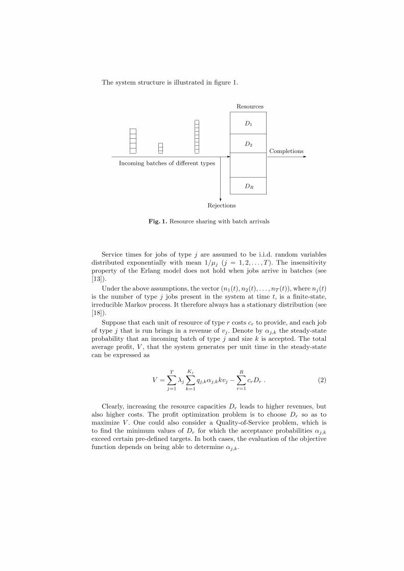
The system structure is illustrated in figure 1.

- -

?Rejections

Completions

Resources

Incoming batches of different types

D1

D2

DR

Fig. 1. Resource sharing with batch arrivals

Service times for jobs of type j are assumed to be i.i.d. random variablesdistributed exponentially with mean 1/µj (j = 1, 2, . . . , T ). The insensitivityproperty of the Erlang model does not hold when jobs arrive in batches (see[13]).

Under the above assumptions, the vector (n1(t), n2(t), . . . , nT (t)), where nj(t)is the number of type j jobs present in the system at time t, is a finite-state,irreducible Markov process. It therefore always has a stationary distribution (see[18]).

Suppose that each unit of resource of type r costs cr to provide, and each jobof type j that is run brings in a revenue of vj . Denote by αj,k the steady-stateprobability that an incoming batch of type j and size k is accepted. The totalaverage profit, V , that the system generates per unit time in the steady-statecan be expressed as

V =

T∑j=1

λj

Kj∑k=1

qj,kαj,kkvj −R∑r=1

crDr . (2)

Clearly, increasing the resource capacities Dr leads to higher revenues, butalso higher costs. The profit optimization problem is to choose Dr so as tomaximize V . One could also consider a Quality-of-Service problem, which isto find the minimum values of Dr for which the acceptance probabilities αj,kexceed certain pre-defined targets. In both cases, the evaluation of the objectivefunction depends on being able to determine αj,k.

3 An erroneous solution

The technique used in Choudhury et al. [3] is to replace an incoming batch oftype j and size k (when qj,k > 0), by a single macro job that goes through aseries of k queues in tandem: in the first queue it uses kdj,r units of type rresource and is served at rate kµj , regardless of how many other such macrojobs are present; in the second queue it uses (k − 1)dj,r units of resource and isserved at rate (k − 1)µj ; this goes on until queue k, where it uses dj,r units ofresource and is served at rate µj . After that, the macro job departs.

Another interpretation of these queues is to think of of them as having in-finitely many servers. Each ordinary job is served on a separate server and assoon as one of them completes, the remaining macro job moves to the nextqueue.

In this formulation, which is equivalent to the one in terms of batches ofordinary jobs, the system state is a vector of integers [nj,k,s], specifying thenumbers of macro jobs of type j and size k that are now in queue s of their seriesof queues (i.e., they have k + 1 − s ordinary jobs remaining). The authors findthat, for both partial and complete blocking, the probabilities of those vectorssatisfy local balance, and therefore the steady-state distribution has productform:

π(n) = G

T∏j=1

Kj∏k=1

k∏s=1

(λjqj,k)nj,k,s

((k + 1− s)µj)nj,k,snj,k,s!, (3)

where n is the state vector [nj,k,s] and G is a normalization constant.

To demonstrate that this product form does not hold in the case of completeblocking, we offer the following simple counter-example. Take a system with asingle resource type, a single job type, and a single batch size. The resourcecapacity is 4, the resource requirement per job is 1 and the incoming batch sizeis 3. The arrival and service rates are both 1.

There are now 3 queues in series, so the system state is a triple (n1, n2, n3).The feasible states are (0,0,0), (1,0,0), (0,1,0), (0,0,1), (1,0,1), (0,1,1) and (0,0,2).The state (0,2,0), for instance, is not feasible because if there was a macro jobin queue 2, consuming 2 resource units, then a new macro job requiring 3 unitswould not have been admitted.

Consider the two states (0,0,1) and (1,0,1). If (3) is correct, then their sta-tionary probabilities are π(0, 0, 1) = G and π(1, 0, 1) = G/3. Hence, π(0, 0, 1) =3π(1, 0, 1). On the other hand, the only way of leaving state (1,0,1) is by aservice completion, either at queue 1, at rate 3, or at queue 3, at rate 1. Thetotal completion rate is 4. The only way of entering state (1,0,1) is by an ar-rival of a new batch, at rate 1, when the system is in state (0,0,1). Therefore,π(0, 0, 1) = 4π(1, 0, 1). This contradiction demonstrates that the solution (3) isnot correct.

The failure of the product form is due to the fact that, contrary to theassertion in [3], local balance does not hold in the case of complete blocking. Inthe above example, in states (1,0,1) and (0,1,1), a service completion at queue

3 (leading to states (1,0,0) and (0,1,0) respectively), cannot be balanced by anarrival because in either case the new batch would be rejected.

In principle, there might exist a different, as yet undiscovered product formsolution for the complete blocking model. For example, one might explore re-versibility arguments, via the RCAT theorem (see Harrison, [11]). However, giventhe strong connection that is known to exist between reversibility and local bal-ance (e.g., see [2]), we believe that such a search is very unlikely to succeed.

In the absence of a tractable exact solution, we now turn to the task of findingan accurate approximation.

4 A fixed-point approximation

We propose treating each job type as if it was an isolated, one-dimensionalMarkov process taking place within a static environment determined by theother job types. More precisely, when considering jobs of type j, assume that alljobs of other types in the system are consuming a fixed total amount, Zj,r, of typer resource (r = 1, 2, . . . , R). In other words, type j operates in an environmentwhere the available resource of type r is Dr−Zj,r. Hence, the maximum numberof type j jobs that can be admitted, mj , is given by (1), with Dr replaced byDr − Zj,r.

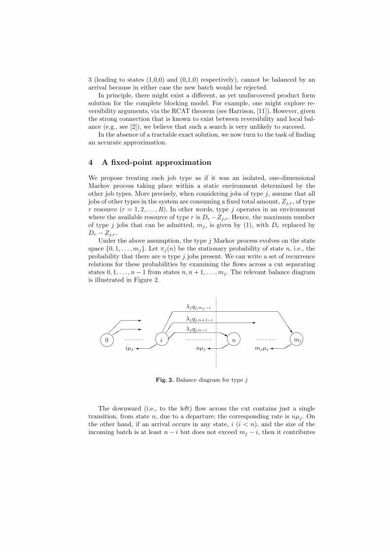
Under the above assumption, the type j Markov process evolves on the statespace {0, 1, . . . ,mj}. Let πj(n) be the stationary probability of state n, i.e., theprobability that there are n type j jobs present. We can write a set of recurrencerelations for these probabilities by examining the flows across a cut separatingstates 0, 1, . . . , n− 1 from states n, n+ 1, . . . ,mj . The relevant balance diagramis illustrated in Figure 2.

���� ���� ��������"" -��

-

���� J

JJJ

""�""�""�

��

-

HHj0 i n mj

iµj mjµjnµj

λjqj,mj−i

λjqj,n+1−i

λjqj,n−i

Fig. 2. Balance diagram for type j

The downward (i.e., to the left) flow across the cut contains just a singletransition, from state n, due to a departure; the corresponding rate is nµj . Onthe other hand, if an arrival occurs in any state, i (i < n), and the size of theincoming batch is at least n− i but does not exceed mj − i, then it contributes

to the upward (to the right) flow across the cut. Equating the two flows providesa balance equation for each n:

nµjπj(n) = λj

n−1∑i=0

πj(i)

mj−i∑k=n−i

qj,k ; n = 1, 2, . . . ,mj . (4)

The simplest way to solve these equations is to set πj(0) = 1, evaluate πj(n)for n = 1, 2, . . . ,mj according to (4), and then re-normalize by dividing each ofthem by their sum.

Having computed the probabilities πj(n), the probability that an incomingbatch of type j and size k is accepted, is given by

αj,k =

mj−k∑n=0

πj(n) . (5)

The average number, Lj , of type j jobs present is equal to

Lj =

mj∑n=1

nπj(n) . (6)

Consequently, the average amount, zj,r, of type r resource consumed by jobsof type j, is given by

zj,r = dj,rLj . (7)

In common with most models of this type, the above solution depends onlyon the ratio ρj = λj/µj , and not on the individual values of those parameters.

We can now approximate the effect that type j has on the other job typesby treating its average consumption of resource r, zj,r as a fixed consumption ofresource r. This will form part of the environment in which another given jobtype operates.

Suppose that we have somehow obtained an estimated vector, L = (L1, L2,. . . , LT ), of the average numbers of jobs of different types in the system. Carryout the following procedure.

1. For every j, compute the type r resource, Zj,r, consumed by job types otherthan j:

Zj,r =

T∑i=1,i6=j

zi,r , (8)

with zi,r being given by (7).2. For every j, use equations (4)—(7) in order to compute new values for Lj ,αj,k and zj,r.

This procedure implements a mapping, f(·), from one vector of averages, callit Lold, to another vector of averages, Lnew. Our approximate solution consists

in finding a vector, L∗, whose ‘new’ image is the same as the ‘old’ one. That is,L∗ is a fixed point of the mapping f(·):

L∗ = f(L∗) . (9)

At the fixed point L∗, the environments in which the different job typesoperate are consistent with each other. That is, for every job type j, the resourcesit consumes, zj,r, do not alter the resources consumed by the other job types,Zj,r. In that sense, this fixed point is like a Nash equilibrium in multi-persongames.

The acceptance probabilities corresponding to L∗ are substituted into (2) inorder to compute the profit V , or are used to see whether the QoS targets havebeen met.

To compute L∗, we use an iterative schema of the form

L(i+1) = f(L(i)) . (10)

These iterations start with some initial vector such as L(0) = (0, 0, . . . , 0),and stop when two consecutive vectors are sufficiently close to each other. Toreduce the number of iterations, it is advisable that the evaluations are of theGauss–Seidel type, i.e. as soon as a new value for some Lj is obtained, thecorresponding value of zj,r is used in determining the environment for other jobtypes.

Note. Fixed-point approximations of queuing systems have been used in thepast, mainly in the context of open or closed networks. There, the decompositionis in terms of nodes and the fixed point equations attempt to capture the inter-actions between them (e.g., see Sadre et al. [21], Whitt [23]). Kelly’s fixed-pointapproximation for multi-class circuit-switched networks [15] is concerned withshared resources, but does not model batch arrivals. The decomposition is withrespect to offered loads for individual units of resource.

As far as we are aware, a decomposition by job type, where the fixed pointequations capture different contributions to a shared environment, has not beenused before.

4.1 Existence and uniqueness of the fixed point

The mapping f(·) is not continuous, because equation (1) involves the ‘floor’function bxc. Consequently, we cannot invoke Brouwer’s theorem and assert theexistence of the fixed point L∗. There are other results that apply to discontinu-ous functions. For example, Hering et al. [12] proved the existence of a fixed pointfor functions that satisfy a property called ‘locally gross direction preserving’. InCromme [4], an approximate fixed point is shown to exist, given certain boundson the discontinuities. In all those cases, checking the conditions of the relevanttheorem requires an explicit characterization of the function whose fixed pointis sought.

Our mapping is defined only by the algorithm that is used to compute it.We know that a small change in Zj,r may cause the maximum number of jobs of

type j, mj , to increase or decrease by 1. However, evaluating the effect of sucha change on the average number of jobs of type j, Lj , is non-trivial. One has tosolve equations (4), and the resulting change may be small or large, dependingon the traffic parameters. For that reason, we have been unable to use existingresults in order to prove the existence of a fixed point.

However, it is possible to give an intuitive reason for the convergence ofiterations (10), by following the evolution of resource allocations. In order to dothat, we need to make some general remarks about average numbers of jobs andoffered loads.

The average offered load of type j is given by σj = λjbj/µj , where bj is theaverage batch size of type j. That would also be the average number of typej jobs present, if all resource capacities were infinite (e.g., see [18]). Hence, theelements of the vectors L are bound by

Lj ≤ σj ; j = 1, 2, . . . , T . (11)

Moreover, the more resources are allocated to type j, the closer Lj is to σj .It is important to bear in mind that real-life clouds are not, on the average,

overloaded. That is, more resources are provided than are required by the averageoffered loads:

T∑j=1

σjdj,r < Dr ; r = 1, 2, . . . , R . (12)

This, together with (11), implies that there are some unconsumed resourcesthroughout the iteration process.

Consider, for simplicity, a single resource system with two job types. Start thefirst iteration with Z1 = 0, i.e. the entire resource, D, is allocated to type 1. Theresulting m1 and L1, take their largest possible values. Type 2 now operatesin an environment where Z2 = L1d1, and the available resource is D − Z2.The corresponding values for m2 and L2 are small. In the second iteration, theresource available to type 1 decreases, causing m1 and L1 to stay the same ordecrease, and m2 and L2 to stay the same or increase. This goes on until, intwo consecutive iterations, m1 remains the same and m2 also remains the same.Then so do L1 and L2, and the process terminates.

In general, with T job types, if in one iteration the allocations of resourcesto certain job types are too generous while the allocations to others are notgenerous enough, there will be a transfer of unconsumed resources from theformer to the latter. In the next iteration, the first set of averages will stay thesame or decrease, while the second will stay the same or increase.

Thus the iterative process naturally pushes the vector L towards a point ofequilibrium.

The fixed point reached by these iterations is not necessarily unique. To seethat, consider the above two-type example under very heavy overload conditions.Suppose that both arrival rates are close to infinity, and assume that all batchesare of size 1 and all resource requirements are 1. If the entire resource, D, isinitially allocated to type 1, then type 1 will consume it all, and the process

will terminate after one iteration, reaching the fixed point (D, 0). If, on theother hand, the entire resource is initially allocated to type 2, then type 2 willconsume it all and the process will terminate after one iteration with the fixedpoint (0, D). In fact, any initial split of the resource will remain unchanged andwill become the final split.

This example is of course unrealistic. We wish to re-emphasize that the sys-tems of practical interest are not overloaded. Indeed, in the experiments thatfollow, the optimal resource capacity that should be provided turns out to bemore than twice as large as the requirement of the average offered load. Undersuch conditions, any fixed point is likely to be close to the true vector L, andtherefore even if there are multiple fixed points, they are likely to be close toeach other.

4.2 Numerical and simulation experiments

To examine the quality of the proposed approximation, consider an examplesystem with four job types, 1, 2, 3 and 4, or ‘small’, ‘medium’, ‘large’ and ‘verylarge’. There is a single resource type and the individual resource requirementsof the four job types are are d1 = 1, d2 = 2, d3 = 4 and d4 = 8. These numbersare motivated by similarities with the T2 family of VM instances offered by theAmazon EC2 (Elastic Computing Cloud) service (see [24]). The resource that isbeing shared in this context is vCPUs (virtual CPUs).

Type 1 jobs arrive singly, at a rate of λ1 = 6 jobs per unit time. Their averageservice times are 1/µ1 = 1. For type 2, the possible batch sizes are 1 or 2, withequal probability (q2,1 = q2,2 = 0.5). The traffic parameters are λ2 = 4 and1/µ2 = 1. Jobs of type 3 and type 4 arrive in batches of size 1, 2, or 3, withprobabilities 0.4, 0.3 and 0.3, respectively. Their arrival and service parametersare λ3 = 2, 1/µ3 = 0.5, λ4 = 1, 1/µ4 = 0.5.

The average offered load requirement for this example, i.e. the left-hand sideof (12), is 33.2 vCPUs.

The cost incurred per unit of resource is c = 0.2, and the revenues brought inby the different job types increase with the resource consumed: v1 = 1, v2 = 3,v3 = 6, v4 = 10.

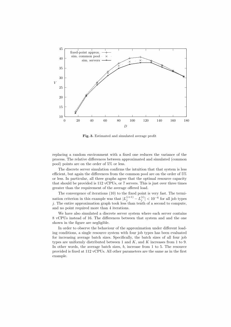
In Figure 3, the estimated average profit is plotted against the offered re-source capacity, D. The three curves correspond to (a) the fixed-point approx-imation, (b) a simulation of the model as described in section 2 and (c) a sim-ulation of a system where the resource is not provided as a common pool, butis contained within servers. In this last case, each server has 16 vCPUs. Thus,in order to offer 128 vCPUs, one has to provide 8 servers. The discrete serversystem is less efficient than the common pool, because, in order to instantiate aVM on a server, all its resource requirement must be available on that server. Itis not enough to have some of the requirement available on one server and someon another.

The two simulation graphs may be considered exact. Their confidence inter-vals are too narrow to plot. The figure shows that the fixed-point approximationtends to overestimate the average profit slightly. This is not surprising, since

10

15

20

25

30

35

40

45

0 20 40 60 80 100 120 140 160 180

V

D

fixed-point approx.

+

+

+

+

+

+ ++

+

+

+

+sim. common pool

×

×

×

×

×× × ×

××

×

×sim. servers

∗

∗

∗

∗

∗∗ ∗ ∗

∗∗

∗

∗

Fig. 3. Estimated and simulated average profit

replacing a random environment with a fixed one reduces the variance of theprocess. The relative differences between approximated and simulated (commonpool) points are on the order of 5% or less.

The discrete server simulation confirms the intuition that that system is lessefficient, but again the differences from the common pool are on the order of 5%or less. In particular, all three graphs agree that the optimal resource capacitythat should be provided is 112 vCPUs, or 7 servers. This is just over three timesgreater than the requirement of the average offered load.

The convergence of iterations (10) to the fixed point is very fast. The termi-

nation criterion in this example was that |L(i+1)j −L(i)

j | < 10−6 for all job typesj. The entire approximation graph took less than tenth of a second to compute,and no point required more than 4 iterations.

We have also simulated a discrete server system where each server contains8 vCPUs instead of 16. The differences between that system and and the oneshown in the figure are negligible.

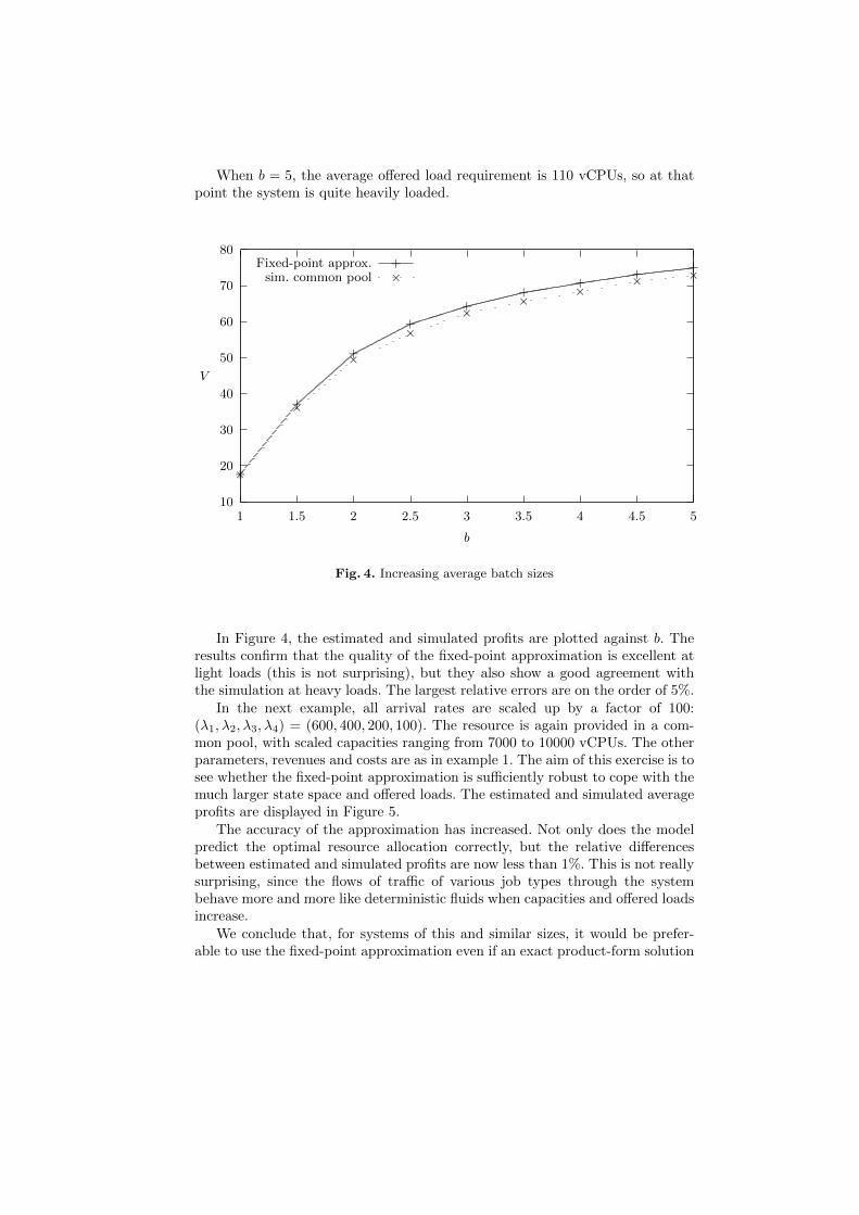
In order to observe the behaviour of the approximation under different load-ing conditions, a single resource system with four job types has been evaluatedfor increasing average batch sizes. Specifically, the batch sizes of all four jobtypes are uniformly distributed between 1 and K, and K increases from 1 to 9.In other words, the average batch sizes, b, increase from 1 to 5. The resourceprovided is fixed at 112 vCPUs. All other parameters are the same as in the firstexample.

When b = 5, the average offered load requirement is 110 vCPUs, so at thatpoint the system is quite heavily loaded.

10

20

30

40

50

60

70

80

1 1.5 2 2.5 3 3.5 4 4.5 5

V

b

Fixed-point approx.

+

+

+

+

++

++

++sim. common pool

×

×

×

××

××

× ××

Fig. 4. Increasing average batch sizes

In Figure 4, the estimated and simulated profits are plotted against b. Theresults confirm that the quality of the fixed-point approximation is excellent atlight loads (this is not surprising), but they also show a good agreement withthe simulation at heavy loads. The largest relative errors are on the order of 5%.

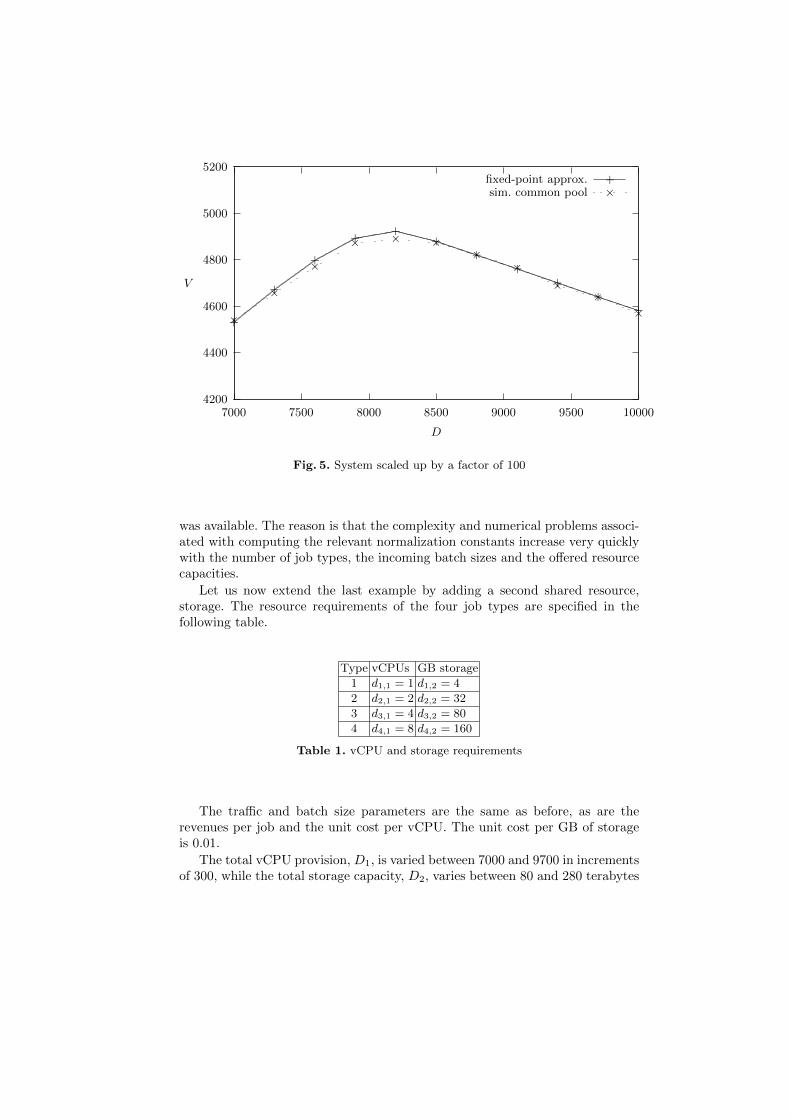
In the next example, all arrival rates are scaled up by a factor of 100:(λ1, λ2, λ3, λ4) = (600, 400, 200, 100). The resource is again provided in a com-mon pool, with scaled capacities ranging from 7000 to 10000 vCPUs. The otherparameters, revenues and costs are as in example 1. The aim of this exercise is tosee whether the fixed-point approximation is sufficiently robust to cope with themuch larger state space and offered loads. The estimated and simulated averageprofits are displayed in Figure 5.

The accuracy of the approximation has increased. Not only does the modelpredict the optimal resource allocation correctly, but the relative differencesbetween estimated and simulated profits are now less than 1%. This is not reallysurprising, since the flows of traffic of various job types through the systembehave more and more like deterministic fluids when capacities and offered loadsincrease.

We conclude that, for systems of this and similar sizes, it would be prefer-able to use the fixed-point approximation even if an exact product-form solution

4200

4400

4600

4800

5000

5200

7000 7500 8000 8500 9000 9500 10000

V

D

fixed-point approx.

+

+

+

++

++

++

++

+sim. common pool

×

×

×

× × ××

××

××

×

Fig. 5. System scaled up by a factor of 100

was available. The reason is that the complexity and numerical problems associ-ated with computing the relevant normalization constants increase very quicklywith the number of job types, the incoming batch sizes and the offered resourcecapacities.

Let us now extend the last example by adding a second shared resource,storage. The resource requirements of the four job types are specified in thefollowing table.

Type vCPUs GB storage

1 d1,1 = 1 d1,2 = 4

2 d2,1 = 2 d2,2 = 32

3 d3,1 = 4 d3,2 = 80

4 d4,1 = 8 d4,2 = 160

Table 1. vCPU and storage requirements

The traffic and batch size parameters are the same as before, as are therevenues per job and the unit cost per vCPU. The unit cost per GB of storageis 0.01.

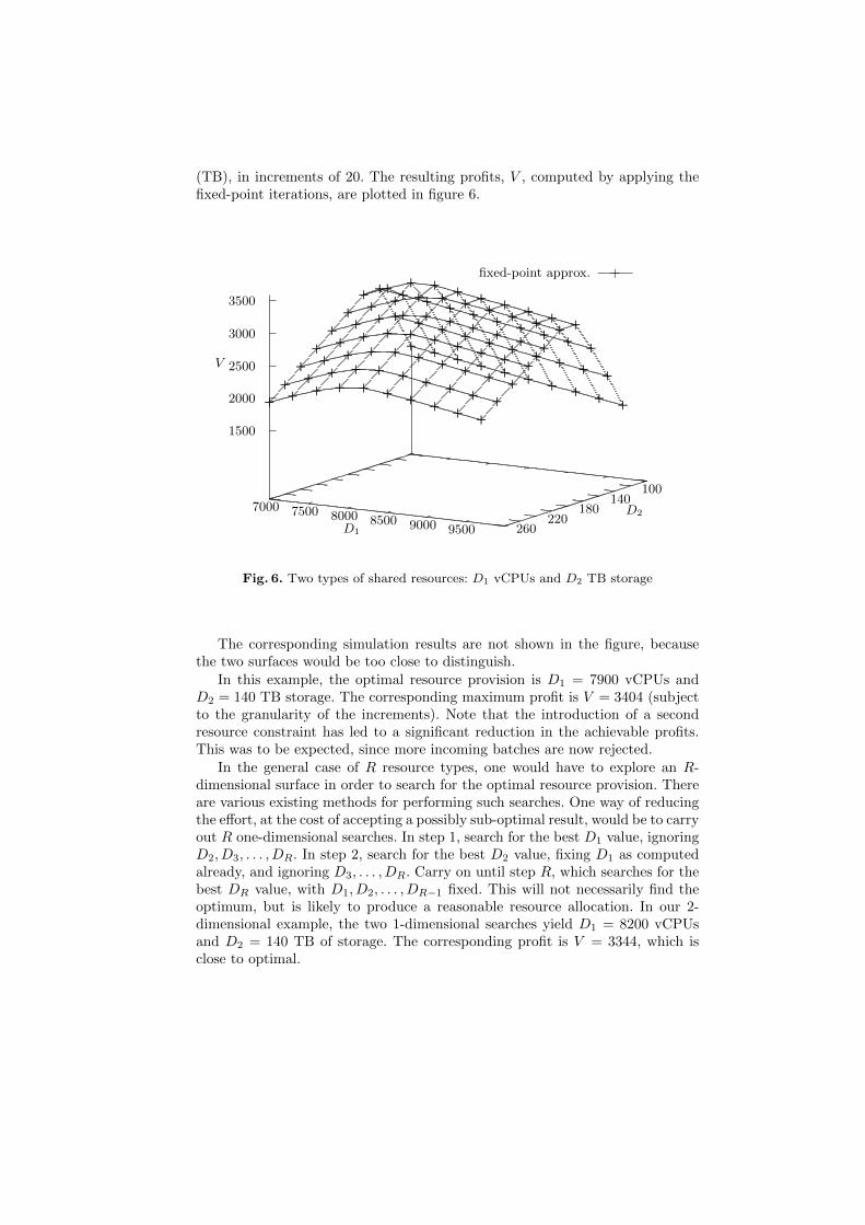
The total vCPU provision, D1, is varied between 7000 and 9700 in incrementsof 300, while the total storage capacity, D2, varies between 80 and 280 terabytes

(TB), in increments of 20. The resulting profits, V , computed by applying thefixed-point iterations, are plotted in figure 6.

100140

180220

260

7000 7500 8000 8500 9000 9500

1500

2000

2500

3000

3500

V

fixed-point approx.

+

+

+

++

+

+

+

+

+

+

+

+

++

+

+

+

+

+

+

+

+

++

+

+

+

+

+

+

+

+

++

+

+

+

+

+

+

+

+

++

+

+

+

+

+

+

+

+

++

+

+

+

+

+

+

+

+

++

+

+

+

+

+

+

+

+

+

+

+

+

+

+

+

+

+

++

+

+

+

+

+

+

+

+

++

+

+

+

+

+

+

++

++++++++ ++

++++++++ +

++

+++++++ +

+++

++++++ ++

++

++++++ ++

++++++++

++

+++

+++++

++

++

++

++

++

+++

++

++

++

+

++

+++

++

++

+

+

D2

D1

Fig. 6. Two types of shared resources: D1 vCPUs and D2 TB storage

The corresponding simulation results are not shown in the figure, becausethe two surfaces would be too close to distinguish.

In this example, the optimal resource provision is D1 = 7900 vCPUs andD2 = 140 TB storage. The corresponding maximum profit is V = 3404 (subjectto the granularity of the increments). Note that the introduction of a secondresource constraint has led to a significant reduction in the achievable profits.This was to be expected, since more incoming batches are now rejected.

In the general case of R resource types, one would have to explore an R-dimensional surface in order to search for the optimal resource provision. Thereare various existing methods for performing such searches. One way of reducingthe effort, at the cost of accepting a possibly sub-optimal result, would be to carryout R one-dimensional searches. In step 1, search for the best D1 value, ignoringD2, D3, . . . , DR. In step 2, search for the best D2 value, fixing D1 as computedalready, and ignoring D3, . . . , DR. Carry on until step R, which searches for thebest DR value, with D1, D2, . . . , DR−1 fixed. This will not necessarily find theoptimum, but is likely to produce a reasonable resource allocation. In our 2-dimensional example, the two 1-dimensional searches yield D1 = 8200 vCPUsand D2 = 140 TB of storage. The corresponding profit is V = 3344, which isclose to optimal.

Although the fixed-point approximation is accurate and efficient, there arelimits to its applicability. For example, if the system in Figure 5 is scaled upby another factor of 10, bringing the arrival rates to (λ1, λ2, λ3, λ4) = (6000,4000, 2000, 1000) and the vCPU resource capacities in the region of 100000, oursolution breaks down. The failure is not in the fixed-point iterations, but in theone-dimensional solutions (4). When the maximum number of jobs, mj , becomestoo large, the implementation of (4) starts to experience numerical overflows.

It is thus desirable to develop another approximation which can be appliedto very large systems and produce reasonable estimates, albeit with some lossof accuracy.

5 Very large-scale systems

We have observed that the solution of an isolated job type ceases to work whenthe resource capacities and the offered loads are on the order of tens of thousandsor more. For such large systems, a simpler and more robust approximation isrequired.

With this in mind, we propose to represent the various batch arrivals of typej by single ‘macro’ jobs with appropriately chosen resource requirements. Then,for the purpose of the fixed-point solution, the isolated type j model becomes aclassic Erlang loss process. The benefit of this simplification is that the Erlang Bfunction, which provides the rejection probability, can be computed in a stablemanner for large values of the parameters.

The arrival rate and average service time of type j macro jobs are λj and1/µj , respectively. To define the resource requirement of type r for a macro jobof type j, δj,r, we take the average over the possible type j batch sizes:

δj,r = dj,r

Kj∑k=1

kqj,k . (13)

Hence, if all other job types consume a fixed amount, Zj,r, of type r resource,then the maximum number of type j macro jobs that can be admitted into thesystem is

mj = minr

{⌊Dr − Zj,r

δj,r

⌋}. (14)

The probability, βj , that an incoming macro job of type j will be rejected, isgiven by the Erlang-B function (e.g., see [18])

βj = B(mj , ρj) =ρmj

j

mj !

[mj∑i=0

ρi

i!

]−1. (15)

A numerically stable procedure for computing the function B(m, ρ) is pro-vided by the recurrence relation

B(m, ρ) =ρmB(m− 1, ρ)

1 + ρmB(m− 1, ρ)

, (16)

starting with B(0, ρ) = 1 (e.g., see [8]).The average number, Lj , of type j macro jobs in the system is then given by

Little’s result:

Lj = ρj(1− βj) . (17)

The average amount of type r resource that those jobs consume is zj,r = Ljδj,r.We now have the necessary elements for carrying out the iterations described

in the previous section and finding the fixed-point vectors of average numbersof macro jobs present, L∗j , and corresponding rejection probabilities, β∗j . Theaverage profit achieved per unit time is given by

V =

T∑j=1

λjvj(1− βj)Kj∑k=1

kqj,k −R∑r=1

crDr . (18)

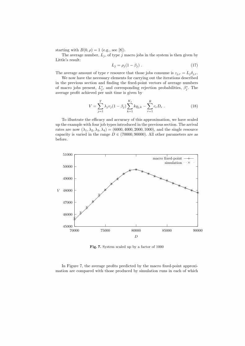
To illustrate the efficacy and accuracy of this approximation, we have scaledup the example with four job types introduced in the previous section. The arrivalrates are now (λ1, λ2, λ3, λ4) = (6000, 4000, 2000, 1000), and the single resourcecapacity is varied in the range D ∈ (70000, 90000). All other parameters are asbefore.

45000

46000

47000

48000

49000

50000

51000

70000 75000 80000 85000 90000

V

D

macro fixed-point

+

+

+

+

+

+

+

+

++ +

++

++

++

++

++

+simulation

××

××

××

××

×× × × ×

× × ×× × ×

× ×

×

Fig. 7. System scaled up by a factor of 1000

In Figure 7, the average profits predicted by the macro fixed-point approxi-mation are compared with those produced by simulation runs in each of which

a total of ten million batches of all types and sizes arrived into the system.Computing the fixed-point was very fast and free from numerical problems. Thesimulation runs were several orders of magnitude slower, because we wantednarrow confidence intervals.

The figure shows that the simplified approximation is remarkably accurate atthis scale. The two plots are almost indistinguishable. This confirms the tendencyobserved earlier, that as the scale of the system increases, its behaviour agreesmore closely with the deterministic assumptions that underlie the fixed-pointapproach.

The above observation applies also when more than one type of resource arebeing shared.

6 Partial blocking

Under the partial blocking policy, the model has a product-form solution (e.g.,see [14]). The system state is described by the vector n = (n1, n2, . . . , nT ), wherenj is the number of jobs of type j present. The feasible states are those satisfyingall resource bounds, i.e.

T∑j=1

njdj,r ≤ Dr ; r = 1, 2, . . . , R . (19)

The stationary probabilities, π(n), are then given by

π(n) = G

T∏j=1

pj(nj) , (20)

whereG is a normalization constant. The quantities pj(nj) satisfy one-dimensionalrecurrences whose only difference from (4) is the range of batch sizes admitted:

nµjpj(n) = λj

n−1∑i=0

pj(i)

Kj∑k=n−i

qj,k ; n = 1, 2, . . . ,mj . (21)

In addition, [14] established that when a single resource with total bound Dis shared, the marginal probabilities, ψ(s), that s resource units are currentlyallocated, also satisfy a set of one-dimensional recurrences:

sψ(s) =

T∑j=1

ρjdj

bs/djc∑i=1

ψ(s− idj)Kj∑

k=i−1

qj,k ; s ≤ D , (22)

where dj is the resource requirement for type j.The problem with these exact solutions is that they do not scale well. The

normalization constant appearing in (20) is difficult to calculate even for modera-tely-sized systems. The recurrences (22) are more efficient, but they too are of

limited utility. As well as only applying to a single shared resource, we haveobserved that those recurrences break down numerically when D is greater thanabout 3000.

In view of these drawbacks, it is advisable to apply a fixed-point approxi-mation to the partial blocking policy. The iterative procedure is as described insection 4. The recurrences (21) are used to compute the one-dimensional distri-bution of type j jobs present, given the resource capacities available to them.This provides a mapping, Lnew = f(Lold), from an old vector of average num-bers of jobs present to a new one. That mapping is iterated until it converges toa fixed point.

At this point one needs to consider the reward structure associated with thepartial blocking policy. In particular, there may be penalties for being unable toallocate all the jobs in an incoming batch. Suppose that, if a batch of type j andsize k is fully allocated, then the revenue received is kvj , but if only i of the kjobs are accepted, then the revenue is iwj , for some wj which would typically beless than vj . Then the contribution of type j to the revenues received, Vj , hastwo terms: revenues received from fully accepted batches and revenues receivedfrom partially accepted batches.

Vj = λj

Kj∑k=1

qj,k

kvj mj−k∑n=0

p(n) + wj

k−1∑i=1

ip(mj − i)

. (23)

It seems intuitively clear that the differences between the complete and par-tial blocking policies would become more pronounced when the batch sizes arelarger and the resource capacities are less generous. To quantify that observation,we shall take the single resource, 4-type example of section 4 and modify it by in-creasing the upper batch limits by a factor of 5: (K1,K2,K3,K4) = (3, 10, 15, 15).Within those limits, the batch sizes are distributed uniformly, which means thatthe variances have also been increased. The arrival rates are now (λ1, λ2, λ3, λ4)= (120, 80, 40, 20). Consequently, in terms of offered loads, this example is similarto the one in figure 5.

The resource requirements, revenues from fully accepted batches and unitcost per vCPU are as before. However, we now assume that if a batch is onlypartially accepted, then the revenue from each of its jobs is half of what it wouldbe if the batch was fully accepted: wj = 0.5vj , j = 1, 2, 3, 4.

The three plots in figure 8 show the profits achieved according to (a) fixed-point approximation of the complete blocking policy, (b) fixed-point approxima-tion of the partial blocking policy and (c) simulated partial blocking where eachpoint corresponds to a run containing one million batch arrivals.

We see that the partial blocking policy is also very accurately approximatedby the fixed-point iterations. The relative errors, as compared with the simula-tions, do not exceed 2%, and are mostly lower than 1%. It is worth remarkingthat the optimal resource allocation (7000 vCPUs, subject to the granularity ofthe increments) is the same for the complete and partial blocking policies.

As expected, when the resource provision is plentiful, there is very littledifference between the two policies. That would be true even if the revenue

2200

2400

2600

2800

3000

3200

3400

3600

3800

4000

4000 4500 5000 5500 6000 6500 7000 7500 8000 8500 9000

V

D

FP complete blocking

+

+

+

+

+

++

++ + +

++

++

+

+FP partial blocking

×

×

×

×

×

×

××

× × × × × × × ×

×Sim partial blocking

∗

∗

∗

∗

∗

∗

∗∗

∗ ∗ ∗ ∗∗ ∗ ∗

∗

∗

Fig. 8. Complete and partial blocking; larger batches

from partially accepted batches was 0. Significant differences begin to emergewhen the resource provided is not enough. With our cost structure, the completeblocking policy is more profitable than the partial blocking one. This is becausethe acceptance of partial batches reduces the probability of accepting full ones,which reduces revenues.

Devising a simple approximation for very large systems is more problematicin the case of the partial blocking policy. Because of the possibility of acceptingparts of batches, and the attendant revenue complications, we need to considerboth macro jobs (aggregated batches) and individual jobs. The latter will betreated as arriving in Poisson streams where the rate for type j, γj , is

γj = λj

Kj∑k=1

kqj,k . (24)

The offered load for individual jobs of type j is σj = γj/µj . For a given resourcecapacity of type r available to type j, Dr − Zj,r, the maximum number of typej jobs that can be present in the system, nj , is equal to

nj = minr

{⌊Dr − Zj,r

dj,r

⌋}, (25)

where dj,r is the type r resource requirement of a type j job.

The fixed-point iterations applied to individual jobs provide the probabilities,βj , that a job of type j is rejected:

βj = B(σj , nj) . (26)

Also, the average number of type j jobs present, and the resources of type r thatthey use, are given by

Lj = σj(1− βj) ; zj,r = Ljdj,r .

It remains to assess the average revenue, uj , that an accepted job of type jwould bring. We propose to use a linear combination

uj = αjvj + (1− αj)wj , (27)

where αj is the probability that the job belongs to a fully accepted batch. Anapproximation for αj is provided by the probability that an aggregated ‘macro’job of type j is accepted:

αj = 1−B(ρj ,mj) , (28)

where ρj = λj/µj is the offered load of type j macro jobs and mj is theirmaximum number, given by (14). Note that the available resources have alreadybeen computed.

The average profit achieved per unit time is now obtained from

V =

T∑j=1

γj(1− βj)uj −R∑r=1

crDr . (29)

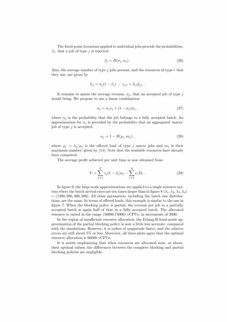
In figure 9, the large-scale approximations are applied to a single resource sys-tem where the batch arrival rates are ten times larger than in figure 8 (λ1, λ2, λ3, λ4)= (1200, 800, 400, 200). All other parameters, including the batch size distribu-tions, are the same. In terms of offered loads, this example is similar to the one infigure 7. When the blocking policy is partial, the revenue per job in a partiallyaccepted batch is again half of that in a fully accepted batch. The allocatedresource is varied in the range (50000,74000) vCPUs, in increments of 2000.

In the region of insufficient resource allocation, the Erlang-B fixed-point ap-proximation of the partial blocking policy is now a little less accurate, comparedwith the simulations. However, it is orders of magnitude faster, and the relativeerrors are still about 5% or less. Moreover, all three plots agree that the optimalresource allocation is 66000 vCPUs.

It is worth emphasizing that when resources are allocated near, or above,their optimal values, the differences between the complete blocking and partialblocking policies are negligible.

26000

28000

30000

32000

34000

36000

38000

40000

50000 55000 60000 65000 70000 75000

V

D

FP complete blocking

+

+

+

++

++

+ + ++

++

+FP partial blocking

×

×

×

×

×

×

×

× × × × × ××

Sim partial blocking

∗

∗

∗

∗

∗

∗∗

∗ ∗ ∗∗ ∗

∗∗

Fig. 9. Large system, complete and partial blocking

7 Conclusion

We have addressed a practically relevant problem concerned with service provi-sioning in public clouds. The multi-class model with batch arrivals and completeblocking appeared to be solved, but we have shown that the existing solution isincorrect. An alternative solution based on fixed-point iterations is introduced.This replaces the multi-dimensional stochastic process with a number of single-dimensional ones, using averages to model the interactions between them. Theaccuracy of the fixed-point solution is good for small systems, and gets betterwhen the system size increases. A simplified version of that solution is shown toapply to very large-scale systems.

The partial blocking model can be solved exactly, but that solution does notscale well. We have therefore applied the approximation methodology and shownit to produce accurate results.

The exact solution of the complete blocking model is still an open problem, asis also the solution of the model where resources are provided in discrete servers,rather than in common pools. Those problems are interesting and worthy offurther study. However, we feel that even if the exact solutions were available,it would be better to tackle the task of optimizing a real-life system by usingthe proposed approximations. They are easily implementable and sufficientlyaccurate.

Other, more general models may be tackled by the methods described here.For example, the complete blocking and partial blocking policies need not be

mutually exclusive. One may wish to operate a mixed policy where some jobtypes are subject to complete blocking, while others are accepted under partialblocking. The fixed-point approach and the large-scale simplifications would stillapply.

References

1. P. Bodık, R. Griffith, C. Sutton, A. Fox, M. Jordan and D. Patterson, “Statisticalmachine learning makes automatic control practical for internet datacenters”, Conf.on Hot Topics in Cloud Computing (HotCloud’09), Berkeley, CA, USA, 2009.

2. X. Chao and M. Miyazawa, “On Quasi-Reversibility and Local Balance: An Alter-native Derivation of the Product-Form Results”, Operations Research, 46, 6, pp.927-933, 1998.

3. G.L. Choudhury, K.K. Leung and W. Whitt, “Resource-sharing models with state-dependent arrivals of batches”, in Computations with Markov Chains (ed. W.J.Stewart), Kluwer, pp. 225-282, 1995.

4. L.J. Cromme, “Fixed point theorems for discontinuous functions and applications”,Nonlinear Analysis: Theory, Methods and Applications, 30, 3, pp. 1527-1534, 1997.

5. J. Dean and S. Ghemawat, “MapReduce: Simplified data processing on large clus-ters”, Communications of the ACM, 51, 1, pp. 107-113, 2008.

6. E.A. van Doorn and F.J.M Planken, “Blocking probabilities in a loss system witharrivals in geometrically distributed batches and heterogeneous service require-ments”, ACM/IEEE Trans. on Networking, 1, pp. 664-667, 1993.

7. P. Ezhilchelvan and I. Mitrani, “Static and Dynamic Hosting of Cloud Servers”,Computer Performance Engineering LNCS 9272, Eds. M. Beltran, W. Knottenbeltand J. Bradley), Springer, 2015.

8. P. Ezhilchelvan and I. Mitrani, “Optimal provisioning of servers for hosting servicesof multiple types”, Simulation Modelling Practice and Theory, 75, pp. 17-28, 2017.

9. P. Ezhilchelvan and I. Mitrani, “Multi-class resource sharing with batch arrivalsand complete blocking”, 14th Int. Conf. on Quantitative Evaluation of SysTems(QEST 2017), Berlin, 2017.

10. R.C. Hampshire, W.A. Massey, D. Mitra and Q. Wang, “Provisioning for Band-width Sharing and Exchange”, in Telecommunications Network Design and Man-agement, vol. 23 of series Operations Research/Computer Science Interfaces,Springer, pp. 207-225, 2003.

11. P.G. Harrison, “Reversed processes, product forms and a non-product form”, Lin-ear Algebra and its Applications, 386, pp. 359-381, 2004.

12. P.J.-J Herings, G. van der Laanb, D. Talmanc, Z. Yang “A fixed point theorem fordiscontinuous functions”, Operations Research Letters, 36, 1, pp. 89-93, 2008.

13. J.S. Kaufman, “Blocking in a shared resource environment”, IEEE Trans. Com-mun., 29, pp. 1474-1481, 1981.

14. J.S. Kaufman and K.M. Rege, “Blocking in a shared resource environment withbatched Poisson arrival processes”, Performance Evaluation, 24, pp. 249-263, 1996.

15. F. Kelly, “Blocking probabilities in large cirquit switched networks”, Advances inApplied Probability, 18, pp. 473-505, 1986.

16. M. Mazzucco, D. Dyachuk, and M. Dikaiakos, “Profit-aware server allocation forgreen internet services”, IEEE Int. Symp. on Modeling, Analysis and Simulationof Computer and Telecommunication Systems (MASCOTS), pp. 277-284, 2010.

17. M. Mazzucco, M. Vasar, and M. Dumas, “Squeezing out the cloud via profit-maximizing resource allocation policies”, IEEE Int. Symp. on Modeling, Analysisand Simulation of Computer and Telecommunication Systems (MASCOTS), pp.19-28, 2012.

18. I. Mitrani, Probabilistic Modelling, Cambridge University Press, 1998.19. J.W. Roberts, “A service system with heterogeneous user requirement”, in Perfor-

mance of Data Communications Systems and Their Applications, (Ed. G. Pujolle),North-Holland, pp. 423-431, 1981.

20. K.W. Ross, Multiservice Loss Models for Broadband Telecommunication Networks,Springer-Verlag, 1995.

21. R. Sadre, B.R. Haverkort and A. Ost. “An efficient and accurate decompositionmethod for open finite- and infinite-buffer queueing networks”, Proc. 3rd Int. Work-shop on Numerical Solution of Markov Chains (Eds. W. Stewart and B. Plateau),pp. 1-20, 1999.

22. Y. Tan, Y. Lu and C.H. Xia, “Provisioning for large scale loss network systems withapplications in cloud computing”, ACM SIGMETRICS Performance EvaluationReview, 40(3), pp. 83-85, 2012.

23. W. Whitt, “The Queueing Network Analyzer”, Bell System Technical Journal,62(9), pp. 2779-2815, 1983.

24. https://aws.amazon.com/ec2/instance-types/ , Amazon Web Services, 2016.