Multi-criteria inventory classification through integration of fuzzy analytic hierarchy process and artificial neural network
Golam Kabir* and M. Ahsan Akhtar Hasin Department of Industrial and Production Engineering (IPE), Bangladesh University of Engineering and Technology (BUET), Dhaka 1000, Bangladesh E-mail: [email protected] E-mail: [email protected] *Corresponding author
Abstract: A systematic approach to the inventory control and classification may have a significant influence on company competitiveness. In practice, all inventories cannot be controlled with equal attention. To efficiently control the inventory items and to determine the suitable ordering policies for them, multi-criteria inventory classification is used. The objective of this research is to develop a multi-criteria inventory classification model through integration of fuzzy analytic hierarchy process (FAHP) and artificial neural network approach. FAHP is used to determine the relative weights of the attributes or criteria using Chang’s extent analysis and to classify inventories into different categories. Various structures of multi-layer feed-forward back-propagation neural networks have been analysed and the optimal one with the minimum mean absolute percentage of error between the measured and the predicted values have been selected. To accredit the proposed model, it is implemented for 351 raw materials of switchgear section of Energypac Engineering Limited, a large power engineering company of Bangladesh.
Reference to this paper should be made as follows: Kabir, G. and Hasin, M.A.A. (2013) ‘Multi-criteria inventory classification through integration of fuzzy analytic hierarchy process and artificial neural network’, Int. J. Industrial and Systems Engineering, Vol. 14, No. 1, pp.74–103.
Biographical notes: Golam Kabir is an Assistant Professor in the Department of Industrial and Production Engineering at Bangladesh University of Engineering and Technology (BUET), Dhaka, Bangladesh. He received a BSc and an MSc in Industrial and Production Engineering from Bangladesh University of Engineering and Technology (BUET) in 2009 and 2011, respectively. His research interest includes multi-criteria decision analysis under risk and uncertainty, fuzzy inference system, mathematical modelling and production optimisation.
M. Ahsan Akhtar Hasin received a BSc in Electrical and Electronics Engineering from BUET, Dhaka, Bangladesh, an MSc in Engineering and a PhD from Industrial Systems Engineering, AIT, Bangkok, Thailand. He has
Multi-criteria inventory classification through integration of FAHP and ANN 75
22 years of teaching and research experience in Bangladesh. He has to his credit a large number of international journal publications and has authored several books and chapters in books, published from USA and other countries.
1 Introduction
Inventory has been looked at as a major cost and source of uncertainty due to the volatility within the commodity market and demand for the value-added product. Inventory is held by manufacturing companies for a number of reasons, such as to allow for flexible production schedules and to take advantage of economies of scale when ordering stock (Nahmias, 2004). The efficient management of inventory systems is therefore a crucial element in the operation of any production or manufacturing company (Chase et al., 2006). Classification of inventory is a crucial element in the operation of any production company. Because of the huge number of inventory items in many companies, great attention is directed to inventory classification into the different classes, which consequently require the application of different management tools and policies (Wild, 2002). ABC inventory management deals with classification of the items in an inventory in decreasing order of annual dollar volume. The ABC classification process is an analysis of a range of items, such as finished products or customers into three categories: A – outstandingly important, B – of average importance, C – relatively unimportant as a basis for a control scheme. Each category can and sometimes should be handled in a different way, with more attention being devoted to category A, less to B and less to C (Muller, 2003).
Sometimes, only one criterion is not a very efficient measure for decision-making. Therefore, multiple criteria decision-making methods are used (Flores and Whybark, 1986, 1987). Apart from other criteria such as lead time of supply, part criticality, availability, stock-out penalty costs, ordering cost, scarcity, durability, substitutability, reparability, etc. have been taken into consideration (Flores and Whybark, 1986, 1987; Zhou and Fan, 2007). More studies have been done on multi-criteria inventory classification in the past 20 years. So, many different methods for classifying inventory and taking into consideration multiple criteria have been used and developed (Cebi et al., 2010; Chu et al., 2008; Guvenir and Erel, 1998; Hadi-Vencheh, 2010; Jamshidi and Jain, 2008; Lei et al., 2005; Ng, 2007; Partovi and Anandarajan, 2002; Ramanathan, 2006; Yu, 2011; Zhou and Fan, 2007).
Flores and Whybark (1986, 1987) proposed the bi-criteria matrix approach, wherein annual dollar usage by a joint-criteria matrix is combined with another criterion. Though this approach is interesting, it accompanies some limitations. Their approach becomes increasingly complicated for three or more criteria to classify inventory items and also weights of all criteria taken into account equal. Flores et al. (1992) have proposed the use of joint-criteria matrix for two criteria. The resulting matrix requires the development of nine different policies and for more than two criteria it becomes impractical to use the procedure. Analytic hierarchy process (AHP) developed by Saaty (1980) has been successfully applied to multi-criteria inventory classification by Flores et al. (1992). The advantage of the AHP is that it can incorporate many criteria and ease of use on a massive accounting and measurement system, but its shortcoming is that a significant amount of subjectivity is involved in pair-wise comparisons of criteria. They have used
76 G. Kabir and M.A.A. Hasin
the AHP to reduce multiple criteria to a univariate and consistent measure. However, Flores et al. (1992) have taken average unit cost and annual dollar usage as two different criteria among others. The problem with this approach is that the annual dollar usage and the unit price of items are usually measured in different units. On the other hand, for the applicability of this approach, the unit of a criterion must not change from item to item.
Partovi and Burton (1993) applied the AHP to inventory classification to include both quantitative and qualitative evaluation criteria. AHP has been praised for its ease of use and its inclusion of group opinions; however, the subjectivity resulting from the pair-wise comparison process of AHP poses problems. Braglia et al. (2004) integrated decision diagram with a set of AHP models used to solve the various multi-attribute decision sub-problems at the different levels/nodes of the decision tree. An inventory policy matrix is defined to link the different classes of spare parts with the possible inventory management policies so as to identify the ‘best’ control strategy for the spare stocks.
Artificial intelligence (AI) methods such as neural networks (NNs), fuzzy logic and genetic algorithms (GAs) are applied for multi-criteria inventory classification. An AI concept is based on the development of the intelligent computer systems with properties similar to human intelligence. Guvenir and Erel (1998) applied GA technique to the problem of multiple criteria inventory classification. Their proposed method is called GA for multi-criteria inventory classification and it uses GA to learn the weights of criteria. Partovi and Anandarajan (2002) proposed an artificial neural network (ANN) approach for inventory classification. ANN is another AI-based technique, which is applicable to the classification process. In their approach, two type of learning method, namely back-propagation and generic algorithms are used to examine the ANN classification power and then their results are compared with together. Their approach finds and brings out non-linear relationships and interactions between criteria. However, as authors have asserted, a number of criteria are restricted, also entering many qualitative criteria into model may be difficult and in addition, learning their meta-heuristics approach is difficult for inventory managers. Lei et al. (2005) compared principal component analysis with a hybrid model combining principal component analysis with ANN and back-propagation algorithm. Šimunović et al. (2009) investigated the application of NNs in multiple criteria inventory classification. Various structures of a back-propagation NN have been analysed and the optimal one with the minimum root mean square error was selected. The predicted results are compared to those obtained by the multiple criteria classification using the AHP.
Ramanathan (2006) proposed a weighted linear optimisation model for multiple criteria ABC (MCABC) inventory classification, where performance score of each item obtained using a data envelopment analysis (DEA)-like model. In the proposed approach, a weighted additive function is used to aggregate the performance of an inventory item in terms of different criteria to a single score, called the optimal inventory score of an item. The weights are chosen using optimisation subject to the constraints that the weighted sum, computed using the same set of weights, for all the items must be less than or equal to one. However, his model may result in a position in which an item with a high value in an unimportant criterion is inappropriately classified as class A. This drawback was rectified by Zhou and Fan (2007) via obtaining most favourable and least favourable scores for each item. Ng (2007) proposes a weighted linear model for MCABC inventory classification. Via a proper transformation, the Ng model can obtain the scores of inventory items without a linear optimiser. The Ng model is simple and easy to understand. Despite its many advantages, Ng model leads to a situation which the weight
Multi-criteria inventory classification through integration of FAHP and ANN 77
of an item may be ignored. To overcome this drawback, Hadi-Vencheh (2010) proposed a simple non-linear programming model which determines a common set of weights for all the items.
Liu and Huang (2006) present a modified DEA model to address ABC inventory classification. The evaluating process has two steps. Firstly, all criteria data for each item are normalised between [0, 1]. Then, the prior scores for all inventory items are computed using the proposed model. Chen and Qu (2006) used fuzzy quadratic optimisation programme for classifying inventory items by taking care of conflicting attributes such as average unit cost, annual dollar usage, critical factor and lead time. Chu et al. (2008) have suggested a new inventory classification approach called ABC-fuzzy classification (ABC-FC) combining the traditional ABC-FC, which can handle variables with nominal or non-nominal attribute, incorporate manager’s experience, judgement into inventory classification and can be implemented easily. Bhattacharya et al. (2007) developed a distance-based multiple criteria consensus framework utilising the technique for order preference by similarity to ideal solution for ABC analysis. Chen et al. (2008) proposed a case-based distance model for multiple criteria ABC analysis, which has been arisen from Flores et al. method (Flores and Whybark, 1986, 1987). Advantage of this model is that it is easily considered as any finite number of criteria for classification. In this model, criteria weights and sorting thresholds are generated mathematically based on the decision-maker’s assessment of a set of the cases. But information cases are very important and if this information is incorrect, this affect process of classification of other items, also its learning may be difficult for the average manager.
Jamshidi and Jain (2008) addressed MCABC inventory classification to standardise each criterion and weight them for classification. The weight for each criterion is based on simple exponential smoothing weight assignments. With inclusion of weight for each criteria and normalising the data, a score is obtained for each item and the classification is done based on the normalised score. Rezaei (2007) used fuzzy set theory and fuzzy analytical hierarchy process (FAHP) to present a simple and applicable approach for ABC classification of inventory. Conventional AHP seems inadequate to capture decision-maker’s requirements on evaluating alternatives always contain ambiguity and multiplicity of meaning. To model this kind of uncertainty in human preference, fuzzy sets could be incorporated with the pair-wise comparison as an extension of AHP. In this approach, at first-related criteria are selected and determine the weights of these criteria using FAHP. Then, assign a score to each item for each criterion as triangular fuzzy number (TFN) and calculate the final normalised weighted score of each item using fuzzy set theory. Finally, using principle for the comparison of fuzzy numbers, the final scores are compared with each other. Then, all items are classified into three classes according to their final score.
Cakir and Canbolat (2008) proposed an inventory classification system based on the FAHP, a commonly used tool for multi-criteria decision-making problems. They integrated fuzzy concepts with real inventory data and design a decision support system assisting a sensible multi-criteria inventory classification. Cebi et al. (2010) used FAHP for classifying inventory items by taking care of conflicting attributes such as demand, unit cost, substitutability, payment terms and lead time. Hadi-Vencheh and Mohamadghasemi (2011) proposed an integrated FAHP–DEA for MCABC inventory classification. FAHP–DEA methodology uses the FAHP to determine the weights of criteria, linguistic terms to assess each item under each criterion, the DEA method to determine the values of the linguistic terms and the simple additive weighting method to
78 G. Kabir and M.A.A. Hasin
aggregate item scores under different criteria into an overall score for each item. Yu (2011) compared AI-based classification techniques with traditional multiple discriminant analysis (MDA). To test the effectiveness, AI-based techniques include support vector machines (SVMs), back-propagation networks (BPNs) and the k-nearest neighbour algorithm, classification results based on four benchmark techniques are compared. The results show that AI-based techniques demonstrate superior accuracy to MDA. Statistical analysis reveals that SVM enables more accurate classification than other AI-based techniques. The summary of the literature on multi-criteria inventory classification is given in Table 1.
ANNs are one of the most powerful computer modelling techniques, based on statistical approach, which are applicable to the classification process. They are able to maintain accuracy when some data required for complete network function are missing (Abbod et al., 2007). The greatest advantage of ANNs over other modelling techniques is their capability to model complex, non-linear processes without having to assume the form of the relationship between input and output variables (Chau, 2006). Otherwise, FAHP is being used more and more frequently in multi-criteria decision-making because of its simplicity and similarity to human reasoning (Tang and Beynon, 2009). This method is suitable for use in evaluating proposed policies (including tangible and intangible information). Furthermore, the FAHP also allows group decision-making to derive priorities based on sets of pair-wise comparisons (Bolloju, 2001). An improved and more accurate multi-criteria inventory classification model can be developed by integrating FAHP with ANN. Therefore, the main objective of this research is to develop an improved multi-criteria inventory classification model through integration of FAHP and ANN approach. Table 1 Summary of multi-criteria inventory classification studies
Multiple criteria Method used References
Annual dollar usage and criticality class Bi-criteria matrix approach
Flores and Whybark (1986)
Average unit cost and annual dollar usage Bi-criteria matrix approach
Flores and Whybark (1987)
Obsolescence, reparability, criticality and lead time AHP Flores et al. (1992) Demand, unit cost, substitutability, payment terms and lead time
AHP Partovi and Burton (1993)
University stationary inventory: annual cost usage, no. of request for item in a year, lead time and replacabilityExplisive inventory: unit price, no. of request for item in a year, lead time, scarcity, durability, substitutability, reparability, order size requirement, stockability and commonality
GA Guvenir and Erel (1998)
Unit cost, ordering cost, demand and lead time ANN Partovi and Anandarajan (2002)
Inventory constraints, costs of lost production, safety and environmental objectives, strategies of maintenance adopted and logistics aspects of spare parts
AHP Braglia et al. (2004)
Average unit cost, annual dollar usage, critical factor and lead time
Weighted linear optimisation
Ramanathan (2006)
Multi-criteria inventory classification through integration of FAHP and ANN 79
Table 1 Summary of multi-criteria inventory classification studies (continued)
Multiple criteria Method used References Average unit cost, annual dollar usage, critical factor and lead time
Quadratic optimisation programme
Chen and Qu (2006)
Unit cost, lead time, consumption rate, perishability of items and cost of storing of raw materials
Annual dollar usage, average unit cost and lead time Weighted linear model
Ng (2007)
Average unit cost, annual dollar usage, critical factor and lead time
Weighted linear optimisation (extended version of R model)
Zhou and Fan (2007)
Unit price, annual demand, stock ability, lead time and certainty of supply
FAHP Rezaei (2007)
Average unit cost, annual dollar usage, critical factor and lead time
Dominance-based rough set approach
Chen et al. (2008)
Annual dollar usage, number of hits and average value per hit
Exponential smoothing weights
Jamshidi and Jain (2008)
Price/cost, annual demand, blockade effect in case of stock out, availability of the substitute material, lead time and common use
FAHP Cakir and Canbolat (2008)
Annual cost usage, criticality factor, lead time 1 and 2, working days
ANN Šimunović et al. (2009)
Annual dollar usage, average unit cost and lead time Non-linear programming model
Hadi-Vencheh (2010)
Demand, unit cost, substitutability, payment terms and lead time
FAHP
Cebi et al. (2010)
Average unit cost, annual dollar usage, critical factor and lead time
AI Yu (2011)
Annual dollar usage, limitation of warehouse space, average lot cost and lead time
FAHP–DEA Hadi-Vencheh and Mohamadghasemi (2011)
2 Artificial neural network
An ANN, often just called a ‘neural network’, is a mathematical model or computational model based on biological NNs. It consists of an interconnected group of artificial neurons and processes information using a connectionist approach to computation. In most cases, an ANN is an adaptive system that changes its structure based on external or internal information that flows through the network during the learning phase. In more practical terms, NNs are non-linear statistical data modelling tools. They can be used to model complex relationships between inputs and outputs or to find patterns in data (Haykin, 2001).
80 G. Kabir and M.A.A. Hasin
ANNs attempt to mimic the basic operation of the brain. Information is passed between the neurons, and based upon the structure and synapse weights, a network behaviour (or output mapping) is provided. Feed-forward NN (Figure 1) was used to develop models. In this network, the information moves in only one direction, forward, from the input nodes through the hidden nodes (if any) and to the output nodes (Baskar and Ramamoorthy, 2004). The first layer is known as input layer, the last as output layer and any intermediate layer(s) as hidden layer(s). A multiple feed-forward layer can have one or more layers of hidden units. The number of units at the input layer and output layer is determined by the problem at hand. Input layer units correspond to the number of independent variables while output layer units correspond to the dependent variables or the predicted values. While the numbers of input and output units are determined by the task at hand, the numbers of hidden layers and the units in each layer may vary (Chau, 2006). The working principle of feed-forward NN is given as follows:
1 The inputs (e.g. X1, X2, …, Xl) are the activity of collecting data from the relevant sources. These data are fed to the NN.
2 The weights control the effects of the inputs on the neuron. In other words, an ANN saves its information over its links and each link has a weight (e.g. W1, W2, …., Wl). These weights are constantly varied while trying to optimise the relation in between the inputs and outputs. Synaptic weights characterise themselves with their strength (value) which corresponds to the importance of the information coming from each neuron. In other words, the information is encoded in these strength weights.
3 Summation function is to calculate of the net input readings from the processing elements. (e.g. sum = W1X1 + W2X2 + W3X3+ … + WlXl).
4 Transfer (activation) function (f) determines the output of the neuron by accepting the net input (sum = W1X1 + W2X2 + W3X3 + … + WlXl) provided by the summation function.
5 Outputs accept the results of the transfer function and present them either to the relevant processing element or to the outside of the network.
6 Each input has its own weight plus there is an additional weight called bias (b).
Figure 1 A feed-forward ANN with input, output and one hidden layer
Multi-criteria inventory classification through integration of FAHP and ANN 81
Training a NN model essentially means selecting one model from the set of allowed models (or, in a Bayesian framework, determining a distribution over the set of allowed models) that minimises the cost criterion. There are numerous algorithms available for training NN models; most of them can be viewed as a straightforward application of optimisation theory and estimation. Most of the algorithms used in training ANNs are employing some form of gradient descent. This is done by simply taking the derivative of the cost function with respect to the network parameters and then changing those parameters in a gradient-related direction.
3 Fuzzy set theory
Theory of fuzzy sets is quite similar to man’s attitude when facing uncertainties to express inaccurate words, such as ‘approximately’, ‘very’, ‘nearly’, etc. as well as for consistency with subjective judgements of different people due to various interpretations from a subject. Zadeh (1965) came out with the fuzzy set theory to deal with vagueness and uncertainty in decision-making to enhance precision. Thus, the vague data may be represented using fuzzy numbers, which can be further subjected to mathematical operation in fuzzy domain. Thus, fuzzy numbers can be represented by its membership grade ranging between 0 and 1. M is a fuzzy number if and only if M is normal and convex fuzzy set of X. A TFN M is shown in Figure 2.
Figure 2 Triangular fuzzy number ( M )
A TFN is denoted simply as (l/m, m/u) or (l, m, u), that represent the smallest possible value, the most promising value and the largest possible value, respectively. The TFN having linear representation on left and right side can be defined in terms of its membership function as:
0, 1( 1) , 1( 1)( ) ,( )0,
xx x mmxu xM m x uu m
x u
μ
<⎧⎪ −⎪ ≤ ≤
−⎪⎛ ⎞ = ⎨⎜ ⎟ −⎝ ⎠ ⎪ ≤ ≤⎪ −⎪
>⎩
82 G. Kabir and M.A.A. Hasin
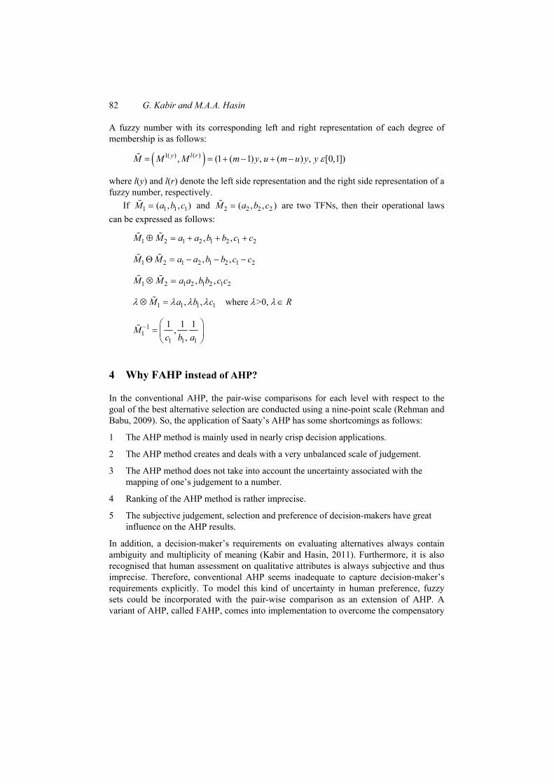
A fuzzy number with its corresponding left and right representation of each degree of membership is as follows:
( )1( ) ( ), (1 ( 1) , ( ) , [0,1])y l rM M M m y u m u y y ε= = + − + −
where l(y) and l(r) denote the left side representation and the right side representation of a fuzzy number, respectively.
If 1 1 1 1( , , )M a b c= and 2 2 2 2( , , )M a b c= are two TFNs, then their operational laws can be expressed as follows:
1 2 1 2 1 2 1 2, ,M M a a b b c c⊕ = + + +
1 2 1 2 1 2 1 2, ,M M a a b b c cΘ = − − −
1 2 1 2 1 2 1 2, ,M M a a b b c c⊗ =
1 1 1 1, , where >0,M a b c Rλ λ λ λ λ λ⊗ = ∈
11
1 1 1
1 1 1,,
Mc b a
− ⎛ ⎞= ⎜ ⎟⎝ ⎠
4 Why FAHP instead of AHP?
In the conventional AHP, the pair-wise comparisons for each level with respect to the goal of the best alternative selection are conducted using a nine-point scale (Rehman and Babu, 2009). So, the application of Saaty’s AHP has some shortcomings as follows:
1 The AHP method is mainly used in nearly crisp decision applications.
2 The AHP method creates and deals with a very unbalanced scale of judgement.
3 The AHP method does not take into account the uncertainty associated with the mapping of one’s judgement to a number.
4 Ranking of the AHP method is rather imprecise.
5 The subjective judgement, selection and preference of decision-makers have great influence on the AHP results.
In addition, a decision-maker’s requirements on evaluating alternatives always contain ambiguity and multiplicity of meaning (Kabir and Hasin, 2011). Furthermore, it is also recognised that human assessment on qualitative attributes is always subjective and thus imprecise. Therefore, conventional AHP seems inadequate to capture decision-maker’s requirements explicitly. To model this kind of uncertainty in human preference, fuzzy sets could be incorporated with the pair-wise comparison as an extension of AHP. A variant of AHP, called FAHP, comes into implementation to overcome the compensatory
Multi-criteria inventory classification through integration of FAHP and ANN 83
approach and the inability of the AHP in handling linguistic variables. The FAHP approach allows a more accurate description of the decision-making process.
5 Proposed model
5.1 Determination of the weights of criteria
One of the important issues of multi-criteria decision-making is prioritisation of criteria. Determining the importance of weights by managers, especially in terms of issue of MCABC classification, is always subjective in such a way that inventory managers usually select some important criteria and then prioritise them. There are several methods to determine the criteria weights, including AHP, entropy analysis, eigenvector method, weighted least square method and linear programming for multi-dimensions of analysis preference. In this model, the method of FAHP is applied.
Generally, it is impossible to reflect the decision-makers’ uncertain preferences through crisp values. Therefore, FAHP is proposed to relieve the uncertainness of AHP method, where the fuzzy comparisons ratios are used. There are several procedures to attain the priorities in FAHP. The fuzzy least square method (Xu, 2000), method based on the fuzzy modification of the logarithmic least squares method (Boender et al., 1989), geometric mean method (Buckley, 1985), the direct fuzzification of the method of Csutora and Buckley (2001), synthetic extend analysis (Chang, 1996), Mikhailov’s fuzzy preference programming (Mikhailov, 2003) and two-stage logarithmic programming (Wang et al., 2005) are some of these methods. Chang’s extent analysis is utilised in this research to evaluate the focusing problem.
Chang (1992) introduces a new approach for handling pair-wise comparison scale based on TFNs followed by use of extent analysis method for synthetic extent value of the pair-wise comparison (Chang, 1996). The first step in this method is to use TFNs for pair-wise comparison by means of FAHP scale, and the next step is to use extent analysis method to obtain priority weights by using synthetic extent values. The fuzzy evaluation matrix of the criteria was constructed through the pair-wise comparison of different attributes relevant to the overall objective using the linguistic variables and TFNs (Figure 3 and Table 2).
Figure 3 Linguistic variables for the importance weight of each criterion
84 G. Kabir and M.A.A. Hasin
Table 2 Linguistic variables describing weights of the criteria and values of ratings
Linguistic scale for importance
Fuzzy numbers Membership function Domain
Triangular fuzzy scale (l, m, u)
Just equal (1, 1, 1) Equally important
1 µM(x) = (3 − x)/(3 − 1) 1 ≤ x ≤ 3 (1, 1, 3)
µM(x) = (x − 1)/(3 − 1) 1 ≤ x ≤ 3 Weakly important 3 µM(x) = (5 − x)/(5 − 3) 3 ≤ x ≤ 5
(1, 3, 5)
µM(x) = (x − 3)/(5 − 3) 3 ≤ x ≤ 5 Essential or strongly important
5 µM(x) = (7 − x)/(7 − 5) 5 ≤ x ≤ 7
(3, 5, 7)
µM(x) = (x − 5)/(7 − 5) 5 ≤ x ≤ 7 Very strongly important 7 µM(x) = (9 − x)/(9 − 7) 7 ≤ x ≤ 9
If factor i has one of the above numbers assigned to it when compared to factor j, then j has the reciprocal value when compared to i
Reciprocals of above
11
1 1 1
1 1 1, ,Muu m l
− ⎛ ⎞= ⎜ ⎟⎝ ⎠
Source: Bozbura and Beskese (2007).
The following section outlines the Chang’s extent analysis method on FAHP. Let 1 2{ , , , }nX x x x= … be an object set and 1 2{ , , , }mU u u u= … be a goal set. As per Chang
(1992, 1996), each object is taken and analysis for each goal, gi, is performed, respectively. Therefore, m extent analysis values for each object can be obtained as follows:
1 2, , , , 1, 2,3, ,mgi gi giM M M i n=… …
iwhere all the ( 1, 2, , )mgiM j m= … are TFNs whose parameters are, depicting least, most
and largest possible values, respectively, and represented as (a, b, c). The steps of Chang’s extent analysis (Chang, 1992) can be detailed as follows (Bozbura et al., 2007; Kahraman et al., 2003, 2004; Wang et al., 2008):
Step 1 The value of fuzzy synthetic extent with respect to ith object is defined as: 1
1 1 1
m n mj j
i gi gij i j
S M M
−
= = =
⎡ ⎤⎢ ⎥= ⊗⎢ ⎥⎣ ⎦
∑ ∑∑
To obtain 1 i
m jgj
M=∑ , perform the fuzzy addition operation of m extent analysis values
for a particular matrix such that,
1 1 1 1
, ,i
m m m mj
j j jgj j j j
M a b c= = = =
⎛ ⎞⎜ ⎟=⎜ ⎟⎝ ⎠
∑ ∑ ∑ ∑
Multi-criteria inventory classification through integration of FAHP and ANN 85
And to obtain 11 1
[ ] ,i
n m jgi j
M −= =∑ ∑ perform the fuzzy addition operation of
( 1, 2, , )i
mgM j m= … (values such that
1 1 1 1 1
, ,i
n m n n nj
i i igi j i i i
M a b c= = = = =
⎛ ⎞= ⎜ ⎟⎜ ⎟⎝ ⎠
∑∑ ∑ ∑ ∑
And then compute the inverse of the vector such that
1
1 11 1 1
1 1 1, ,i
n mj
g n n ni j i i ii i i
Mc b a
−
= == = =
⎛ ⎞⎡ ⎤ ⎜ ⎟⎢ ⎥ = ⎜ ⎟⎢ ⎥ ⎜ ⎟⎣ ⎦ ⎝ ⎠∑∑
∑ ∑ ∑ Step 2 The degree of possibility of M2 = (a2, b2, c2) ≥ M1 = (a1, b1, c1) is defined as:
( ) ( )1 22 1 sup min ( ), ( )M MV M M x xμ μ⎡ ⎤≥ = ⎣ ⎦ And can be equivalently expressed as follows:
( ) ( )2 1
2 1 1 2 1 2
1 2
2 2 1 1
1, if 0, if
, otherwise( ) ( )
b bV M M hgt M M a c
a cb c b a
⎧⎪ ≥⎪⎪≥ = = ≥⎨⎪ −⎪
− − −⎪⎩
∩
where d is the ordinate of the highest intersection point D between
1Mμ and 2Mμ as
shown in Figure 4.
Figure 4 The intersection between M1 and M2
86 G. Kabir and M.A.A. Hasin
To compare M1 and M2, both the values of V(M1 ≥ M2) and V(M2 ≥ M1).
Step 3 The degree of possibility for a convex fuzzy number to be greater than k convex fuzzy numbers Mi (i = 1,2,…, k) can be defined by,
( ) ( ) ( ) ( )( )
1 2 1 2, , , and and
min , ( 1,2,3, , )k m
i
V M M M M V M M M M M M
V M M i k
⎡ ⎤≥ = ≥ ≥ ≥⎣ ⎦= ≥ =
…
… Assuming that,
( ) ( )min for 1,2,3, , ;i i kd A V S S k n k i′ = ≥ = ≠… Then the weight vector is given by,
( ) ( ) ( )( )T1 2, , , nW d A d A d A′ ′ ′ ′= …
where Ai = (i = 1, 2, 3, …, n) are n elements.
Step 4 By normalising, the normalised weight vectors are
( ) ( ) ( )( )T1 2, , , nW d A d A d A= …
where W is a non-fuzzy number.
5.2 Back-propagation NN
BPNs are the most widely used classification technique for training an ANN. A BPN utilises supervised learning methods and feed-forward architecture to perform complex functions such as pattern recognition, classification and prediction. In the research, back-propagation supervised learning technique used to train the models. Its learning procedure is based on gradient search with least sum squared optimality criterion (Abbod et al., 2007). A typical BPN (Figure 5) is composed of three layers of neurons: the input layer, the hidden layer and the output layer. The input layer is considered the model stimuli, while the output layer is the associated outcome of the stimuli. The hidden layer establishes the relationship between the input and the output layers by constructing interconnecting weights (Yu, 2011).
The essence of the BP learning algorithm is to load the input–output relations (which are represented by data sets) within the multi-layer percentron topologies so that it is trained adequately about the past to generalise the future. During the feed-forward, each input unit receives an input signals and sends the signal to each of the hidden units. The hidden unit then computes its activation and sends its signal to the output units. Each output units computes its activation to form the response of the network for the given input pattern. These estimates are then compared to the desired output, and an error is computed for each given observation (Partovi and Anandarajan, 2002). This error is then transmitted backward from the output layer to each mode of the hidden layer. Each of the hidden nodes receives only a portion of the error, which is based upon the relative contribution of each of the hidden nodes to the given estimate. This process continues until each node has received its error contribution. The weights are then adjusted to converge towards a solution, and the network is considered trained (Šimunović et al., 2009).
Multi-criteria inventory classification through integration of FAHP and ANN 87
Figure 5 Proposed BPN architecture (see online version for colours)
The standard BP algorithm suffers from the serious drawbacks of slow convergence and inability to avoid local minima. Therefore, BP with the Levenberg–Marquardt (LM) approximation is used in most of the work. The LM learning rule uses an approximation of Newton’s method to get better performance (More, 1977).
This technique is relatively faster but requires more memory. The LM update rule is:
( ) 1T TW J J l J eμ−
∇ = +
where J is the Jacobean matrix of derivatives of each error to each weight, µ is a scalar and e is an error vector. If the scalar is very large, the above expression approximates the gradient descent method while if it is small the above expression becomes the Gauss–Newton method. The Gauss–Newton method is faster and more accurate near
88 G. Kabir and M.A.A. Hasin
error minima. Hence, the aim is to shift towards the Gauss–Newton as quickly as possible. The µ is decreased after each successful step and increased only when the step increases the error.
5.2.1 Testing and performance of the NN
Training and testing performance of the optimum network topology can be evaluated by the following measures:
1/221RMSE j j
j
t op
⎛ ⎞⎛ ⎞⎜ ⎟= −⎜ ⎟⎜ ⎟⎝ ⎠⎝ ⎠∑
( )( )
2
221
j jj
jj
t oR
o
⎛ ⎞−⎜ ⎟= − ⎜ ⎟
⎜ ⎟⎝ ⎠
∑∑
((( ) / ) 100)MEP
j j jjt o t
p
− ×=∑
model prediction values experimental valuesAPE% 100%experimental values
−= ×
where
T target value O output value RMSE root mean squared error MEP mean error percentage APE absolute percentage of error R2 coefficient of determination/absolute fraction of variance P number of patterns j processing elements
6 Application of the model
To accredit the proposed model, it is implemented for the 351 raw materials of switchgear section of Energypac Engineering Limited (EEL), one of the leading power engineering companies in Bangladesh. EEL is the manufacturer of transformer (power transformer, distribution transformer and instrumental transformer) and switchgear (outdoor vacuum circuit breaker, indoor vacuum circuit breaker, control, metering and relay panels, low tension and power factor improvement panel, indoor type load break switch, outdoor offload disconnector and by-pass switch). FAHP is used to determine the
Multi-criteria inventory classification through integration of FAHP and ANN 89
relative weights of the attributes or criterions, and ANN is used to classify inventories into different categories through training the data set.
6.1 Determination of criteria
Based on the extensive literature review (Table 1), experts participating in the implementation of this model have regarded five important criteria for classification of inventory. Those are: unit price, annual demand, criticality, last use date and durability.
6.2 Determination of the weights of criteria using FAHP
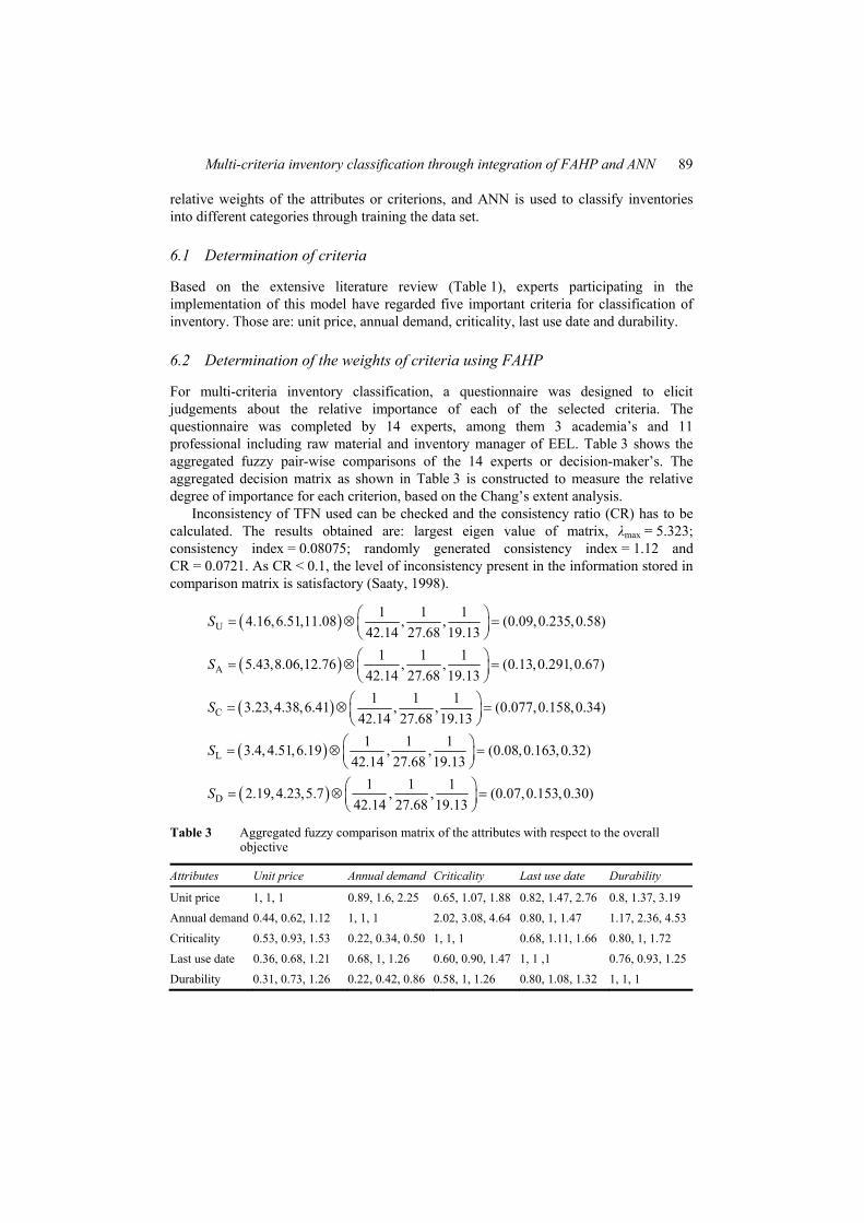
For multi-criteria inventory classification, a questionnaire was designed to elicit judgements about the relative importance of each of the selected criteria. The questionnaire was completed by 14 experts, among them 3 academia’s and 11 professional including raw material and inventory manager of EEL. Table 3 shows the aggregated fuzzy pair-wise comparisons of the 14 experts or decision-maker’s. The aggregated decision matrix as shown in Table 3 is constructed to measure the relative degree of importance for each criterion, based on the Chang’s extent analysis.
Inconsistency of TFN used can be checked and the consistency ratio (CR) has to be calculated. The results obtained are: largest eigen value of matrix, λmax = 5.323; consistency index = 0.08075; randomly generated consistency index = 1.12 and CR = 0.0721. As CR < 0.1, the level of inconsistency present in the information stored in comparison matrix is satisfactory (Saaty, 1998).
The degree of possibility of superiority of SU is calculated and is denoted by V(SU ≥ SA). Therefore, the degree of possibility of superiority for the first requirement, the values are calculated as:
( ) ( )( ) ( )
U A U C
U L U D
0.9 1
1 1
V S S V S S
V S S V S S
≥ = ≥ =
≥ = ≥ =
For the second requirement, the values are calculated as:
( ) ( )( ) ( )
A U A C
A L A D
1 1
1 1
V S S V S S
V S S V S S
≥ = ≥ =
≥ = ≥ =
For the third requirement, the values are calculated as:
( ) ( )( ) ( )
C U C A
C L C D
0.75 0.6
0.98 1
V S S V S S
V S S V S S
≥ = ≥ =
≥ = ≥ =
For the fourth requirement, the values are calculated as:
( ) ( )( ) ( )
L U L A
L C L D
0.75 0.60
1 1
V S S V S S
V S S V S S
≥ = ≥ =
≥ = ≥ =
For the fifth requirement, the values are calculated as:
( ) ( )( ) ( )
D U D A
D C D L
0.70 0.55
0.98 0.96
V S S V S S
V S S V S S
≥ = ≥ =
≥ = ≥ =
The minimum degree of possibility of superiority of each criterion over another is obtained. This further decides the weight vectors of the criteria. Therefore, the weight vector is given as:
(0.9,1, 0.61, 0.60, 0.55)W ′ =
The normalised value of this vector decides the priority weights of each criterion over another. The normalised weight vectors are calculated as:
(0.246,0.273,0.167,0.164,0.15)W =
The normalised weight of each success factor is depicted in Figure 6. Figure 6 show that the annual demand has higher priority than the other criteria. The weights of the criteria represent the ratio of how much more important one criterion is than another, with respect to the goal or criterion at a higher level.
Multi-criteria inventory classification through integration of FAHP and ANN 91
Figure 6 Normalised weights of criteria for multiple criteria inventory classification
Unit Price Annual Demand Criticality Last Use Date Durability0.00
0.05
0.10
0.15
0.20
0.25
0.30W
eigh
ts
Criteria
W eights
6.3 Data collection
Unit price, last year consumption or annual demand, last use date, criticality, durability of 351 materials of switchgear section has been collected. Last date used, durability of the material are transformed to the 0–10 scale and criticality is transformed to the 0–5 scale. Range and value for the transformation of last use date, criticality and durability are shown in Tables 4–6. Table 4 Transformation of last use date
Range Value
Used within a day 10 Used within a week 8 Used within a month 6 Used within 6 months 4 Used within a year 2 Used more than a year 1
>1 week 10 >1 month 8 >6 months 5 >1 year 3 <1 year 1
6.4 Determination of composite priority weights
In FAHP methodology, for a very large number of alternatives (351), making pair-wise comparisons of alternatives, with respect to each criterion, can be time consuming and confusing, because the total number of comparisons will also be very high. Therefore, multiple criteria inventory classification is carried out by using the modified FAHP methodology, which includes pair-wise comparisons of criteria, but not pair-wise comparisons of alternatives. Because of the large number of alternatives (351), pair-wise comparisons of the alternatives are not performed.
Finally, the composite priority weights of each alternative can be calculated by multiplying the weights of each alternative by the data of the corresponding criteria. The composite priority weight of the alternatives gives the idea about the appropriate class of the alternatives or items. Items are ranked according to overall composite priority weights in the descending order. The limits for the classes are derived on the following basis. Class A involves 70% of the total composite priority weights. Class B involves 20% of the total composite priority weights amount of items, while 10% of total composite priority weights belong to class C. The results of the study show that among 351 items, 22 items are identified as class A or very important group or outstandingly important, 47 items as class B or important group or average important and the remaining 282 items as class C or unimportant group or relatively unimportant as a basis for a control scheme.
6.5 Inventory classification by NN
ANNs are one of the most powerful computer modelling techniques, based on statistical approach, currently being used in many fields of engineering for modelling complex relationships which are difficult to describe with physical models. The important criteria for classification of each stock keeping unit. The NN has been designed with MATLAB 7.6 software.
6.5.1 ANN model description
The input/output data set of the ANN model that is going to be formulated to classify items is illustrated schematically in Figure 7. The input parameters of the NN are namely unit price, annual demand, criticality, last use date and durability. The output parameters of the model are three types of inventory items namely A, B and C.
The five basic steps used in general application of NN have been adopted in the development of the model: assembly or collection of data; analysis and pre-processing of
Multi-criteria inventory classification through integration of FAHP and ANN 93
the data; design of the network object; training and testing of the network; and performing simulation with the trained network and post-processing of results.
Figure 7 Schematic diagram of ANN for inventory classification
6.5.2 Collection and pre-possessing of input–output data set
Unit price, last year consumption, last use date, supplier, criticality, durability of 351 materials of switchgear section have been used as input data set, and the class of the item based on the total composite priority weights has been considered as output data set.
The generalisation capability of the NN is totally dependent on:
1 the selection of appropriate input–output parameters of the system
2 the distribution of the data set
3 the format of the presentation of the data set to the network.
Before the ANN can be trained and the mapping learnt, it is important to process the experimental data into patterns. Training and testing pattern vectors are formed before input–output data set are fed to network. Each pattern is formed with an input condition vector, Pi and the corresponding target vector, Ti.
Before training the network, the input–output data set were normalised within the range of ±1, using the Matlab command ‘premnmx’. The normalised value (xi) for each raw input–output data set (di) was calculated as:
( )minmax min
2 1i ix d dd d
= − −−
where
xi = normalised value.
di = original value of input/output.
dmin = minimum value of input/output.
dmax = maximum value of input/output.
94 G. Kabir and M.A.A. Hasin
6.5.3 NN design and training
To find out the best network architecture, different networks with different number of layers and neurons in the hidden layer were designed and tested; transfer functions in the hidden layer and output layer were changed and finally select the optimal network to classify inventories or items. For the optimal network architecture, logarithmic transfer function ‘logsig’ and tangent sigmoid transfer function ‘tansig’ has been used in the hidden layer and logarithmic transfer function ‘logsig’, tangent sigmoid transfer function ‘tansig’, linear transfer function ‘purelin’ has been used in the output layer. For this study, number of hidden neuron was 3, 4, 5, 6, 7, 8, 9, 10, 11, 12, 13, 14, 15 and 16 with 1 or 2 hidden layer.
The performance of the network was evaluated by mean absolute percentage of error (MAPE) and coefficient of determination (R2) between the measured and the predicted values for every output nodes in respect of training the network. The input–output data set consisting of 351 patterns was divided randomly into two categories: training data set which consists of 75% of the data (262 input/output data set) and test data set which consists 25% the data (89 input/output data set). The algorithm used for the NN learning is ‘the backward propagation algorithm’ with LM version. The momentum constant and learning rate used in this model is 0.5 and 0.5, respectively. The maximum number of training epochs set was 10,000 and the training error goal was 0.0001.
The value of R2 and MAPE values between the network predictions and the experimental values using training and test data set for different network architecture have been shown in Table 7. To find out the optimal model, 72 different NN architecture models have been constructed. Table 7 NN architecture for multi-criteria inventory classification
No. of hidden neurons Activation function Train/test error
It is shown from Table 7 that network with 1 hidden layer and 9 neurons in the hidden layer with ‘tansigmoid’ and ‘purelin’ transfer function in the hidden and output layer, respectively, and trained with LM algorithm provides the best result. So, 5–9–3 network architecture was selected as the optimum ANN model. Figure 8 shows that the correlation coefficient of 0.99989 and 0.99971 was obtained for training and testing data set, respectively. Figure 9 shows the ANN prediction values and actual values for 5–9–3 ANN architecture. From the graphs, it is clear that the proposed model can predict values which are nearly very close to experimental observations for each of the output parameters. So, it can be concluded that the model suggested in this work have high accuracy to classify inventories or items. The summary of the proposed model is given in Table 8.
Multi-criteria inventory classification through integration of FAHP and ANN 97
Figure 8 Correlation between ANN prediction and actual values of inventory classification (5–9–3 ANN architecture): (a) training data set; (b) testing data set (see online version for colours)
(a)
(b)
98 G. Kabir and M.A.A. Hasin
Figure 9 Actual vs. ANN prediction of inventory classification (5–9–3 ANN architecture)
All input data normalised between 0 and 1 Performance goal/error goal: 0.0001 Maximum epochs (cycles) set: 10,000 Number of epochs required for: 7
Computation/ termination
Gradient: 0.014459
Multi-criteria inventory classification through integration of FAHP and ANN 99
7 Discussions
Fuzzy linguistic terms has been employed for facilitating the comparisons between the subject criteria, since the decision-makers feel much comfortable using linguistic terms rather than providing exact crisp judgements. Using Chang’s extent analysis, the normalised weight of each attributes is depicted which is shown in Figure 5. Figure 5 shows that the annual demand has higher priority (0.273) than the other criteria. The composite priority weight of each alternative has been calculated using the modified FAHP methodology. The composite priority weight of the alternatives gives the idea about the appropriate class of the alternatives or items. Class A involves 10% of the total composite priority weights. Class B involves 20% of the total composite priority weights amount of items, while 70% of total composite priority weights belong to class C. The results of the study show that among 351 items, 22 items are identified as class A or very important group or outstandingly important, 47 items as class B or important group or average important and the remaining 282 items as class C or unimportant group or relatively unimportant as a basis for a control scheme.
An ANN with feed-forward back-propagation algorithm was trained and the training epoch (cycles) set for each network is 10,000. The input–output data set consisting of 351 patterns was divided randomly into two categories: training data set which consists of 75% of the data (262) and test data set which consists of 25% of the data (89). The numbers of neurons in the hidden layer was found by trial and error method and finally, 9 hidden neurons were chosen for the suggested network. The proposed network can be represented as 5–9–3. The coefficient of determination (R2) was obtained 0.99989 and 0.99971 for training and testing data set, respectively. The MAPE between the actual and the predicted values were 0.0370 for the train data and 0.0791 for the test data.
8 Conclusions
In today’s manufacturing and business environment, an organisation must maintain an appropriate balance between critical stock-outs and inventory holding costs. Because customer service is not a principal factor for attracting new customers, but it is frequently a major reason for losing them. Many researchers have devoted to achieving this appropriate balance. Multi-class classification utilising multiple criteria requires techniques capable of providing accurate classification and processing a large number of inventory items. In this research, a new multi-criteria inventory classification model has been proposed through integration of FAHP and ANN approach.
FAHP technique was used to synthesise the opinions of the decision-makers to identify the weight of each criterion. The FAHP approach proved to be a convenient method in tackling practical multi-criteria decision-making problems. It demonstrated the advantage of being able to capture the vagueness of human thinking and to aid in solving the research problem throu
gh a structured manner and a simple process. The back-propagation learning algorithm has been used in the developed feed-forward single hidden layer network. The input and output vectors were supplied to the network, it was a supervised learning scheme. The back-propagation learning algorithm with LM algorithm versions was used at the training and testing stage of the networks. The result shows that the model can be successfully implemented to classify items or inventories.
100 G. Kabir and M.A.A. Hasin
The classification system is very flexible in the sense that the user:
1 can incorporate some other criteria or remove any criteria for his/her specific implementation
2 can conduct different classification analyses for different inventory records
3 can employ an application-specific linguistic variable set
4 can substitute the crisp comparison values aij for the fuzzy comparison values aij in the optimisation programme, whenever the fuzzy comparisons are not available.
In the multi-criteria inventory classification application, it was found out that the ANN results are significantly consistent with the particular characteristics of the class-altering items. The new inventory classes also suggest the following inventory policies:
Class A:
1 Since the main inventory investment is devoted to class A items, the tightest controlling and auditing levels should be applied to this class.
2 Since most of the items clustered in this class were deemed as ‘critical’, detailed demand forecast reports should be prepared and appropriate levels of safety stock should be maintained.
3 Detailed recording systems should be established (i.e. via automated records, barcode systems, etc.).
Class B:
1 A periodic review policy may be adopted, less detailed forecasts and simpler purchasing procedures can be employed (i.e. economic order quantity may be used).
2 Rational levels of safety stock can be held for the class-altering items those were clustered in class A with a traditional ABC analysis.
Class C:
1 Some of the control and record processes may be ignored.
2 Review periods may be irregularly scheduled.
Further development of FAHP application could be the improvement in the determination of the weights of each component and to handle uncertainty level of the decision environment by using hybrid neuro-fuzzy models, like the quick fuzzy back-propagation algorithm. The use of the ANN tool can be proved to be a persuasive analytical tool in deciding whether an item should be classified as a category A, B or C. However, although these classification models have several advantages, they also have their limitations. Firstly, the number of variables which can be used as inputs to these models was limited. Many new important qualitative variables may be difficult to incorporate into the models. In this research, only feed-forward NN has been considered. The work can also be analysed using recurrent NN or radial basis functional NN and then compared the prediction accuracy or generalisation capability of different types of NN.
Multi-criteria inventory classification through integration of FAHP and ANN 101
Acknowledgements
The authors would like to thank the editor and the anonymous reviewers of IJISE for their constructive and helpful comments.
References Abbod, M.F., Catto, W.F., Derek, A.L. and Freddie, C.H. (2007) ‘Application of artificial
intelligence to the management of urological cancer’, The Journal of Urology, Vol. 178, No. 4, pp.1150–1156.
Baskar, G. and Ramamoorthy, N.V. (2004) ‘Artificial neural network: an efficient tool to simulate the profitability of state transport undertakings’, Indian Journal of Transport Management, Vol. 28, No. 2, pp.243–257.
Bhattacharya, A., Sarkar, B. and Mukherjee, S.K. (2007) ‘Distance-based consensus method for ABC analysis’, Int. J. Production Research, Vol. 45, No. 15, pp.3405–3420.
Boender, C.G.E., de Graan, J.G. and Lootsma, F.A. (1989) ‘Multi-criteria decision analysis with fuzzy pairwise comparisons’, Fuzzy Sets and Systems, Vol. 29, No. 2, pp.133–143.
Bolloju, N. (2001) ‘Aggregation of analytical hierarchy process models based on similarities in decision makers’ preferences’, European Journal of Operational Research, Vol. 128, No. 3, pp.499–508.
Bozbura, F.T. and Beskese, A. (2007) ‘Prioritization of organizational capital measurement indicators using fuzzy AHP’, Int. J. Approximate Reasoning, Vol. 44, No. 2, pp.124–147.
Bozbura, F.T., Beskese, A. and Kahraman, C. (2007) ‘Prioritization of human capital measurement indicators using fuzzy AHP’, Expert Systems with Applications, Vol. 32, No. 4, pp.1100–1112.
Braglia, M., Grassi, A. and Montanari, R. (2004) ‘Multi-attribute classification method for spare parts inventory management’, Journal of Quality in Maintenance Engineering, Vol. 10, No. 1, pp.55–65.
Cakir, O. and Canbolat, M.S. (2008) ‘A web-based decision support system for multi-criteria inventory classification using fuzzy AHP methodology’, Expert Systems with Applications, Vol. 35, No. 3, pp.1367–1378.
Cebi, F., Kahraman, C. and Bolat, B. (2010) ‘A multiattribute ABC classification model using fuzzy AHP’, Proceedings of the 40th International Conference on Computers and Industrial Engineering, Awaji, Japan, 25–28 July.
Chang, D.Y. (1992) ‘Extent analysis and synthetic decision’, Optimization Techniques and Applications, Vol. 1, pp.352–355.
Chang, D.Y. (1996) ‘Applications of the extent analysis method on fuzzy AHP’, European Journal of Operational Research, Vol. 95, No. 3, pp.649–655.
Chase, R.B., Jacobs, F.R., Aquilano, N.J. and Agarwal, N.K. (2006) Operations Management for Competitive Advantage (11th ed.). New York, USA: McGraw Hill.
Chau, K.W. (2006) ‘A review on integration of artificial intelligence into water quality modeling’, Marine Pollution Bulletin, Vol. 52, No. 7, pp.726–733.
Chen, Y., Li, K.W., Kilgour, D.M. and Hipel, K.W. (2008) ‘A case-based distance model for multiple criteria ABC analysis’, Computers & Operations Research, Vol. 35, No. 3, pp.776–796.
Chen, Y. and Qu, L. (2006) ‘Evaluating the selection of logistics centre location using fuzzy MCDM model based on entropy weight’, Proceedings of the 6th World Congress on Intelligent Control and Automation, Dalian, China, 21–23 June.
102 G. Kabir and M.A.A. Hasin
Chu, C.W., Liang, G.S. and Liao, C.T. (2008) ‘Controlling inventory by combining ABC analysis and fuzzy classification’, Computers and Industrial Engineering, Vol. 55, No. 4, pp.841–851.
Csutora, R. and Buckley, J.J. (2001) ‘Fuzzy hierarchical analysis: the Lambda-Max method’, Fuzzy Sets and Systems, Vol. 120, pp.181–195.
Flores, B.E., Olson, D.L. and Dorai, V.K. (1992) ‘Management of multicriteria inventory classification’, Mathematical and Computer Modeling, Vol. 16, No. 12, pp.71–82.
Flores, B.E. and Whybark, D.C. (1986) ‘Multiple criteria ABC analysis’, Int. J. Operations and Production Management, Vol. 6, No. 3, pp.38–46.
Flores, B.E. and Whybark, D.C. (1987) ‘Implementing multiple criteria ABC analysis’, Journal of Operations Management, Vol. 7, No. 1, pp.79–84.
Guvenir, H.A. and Erel, E. (1998) ‘Multicriteria inventory classification using a genetic algorithm’, European Journal of Operational Research, Vol. 105, No. 1, pp.29–37.
Hadi-Vencheh, A. (2010) ‘An improvement to multiple criteria ABC inventory classification’, European Journal of Operational Research, Vol. 201, No. 3, pp.962–965.
Hadi-Vencheh, A. and Mohamadghasemi, A. (2011) ‘A fuzzy AHP-DEA approach for multiple criteria ABC inventory classification’, Expert Systems with Applications, Vol. 38, No. 4, pp.3346–3352.
Haykin, S. (2001) Neural Networks: A Comprehensive Foundation (2nd ed.). Singapore: Pearson Education, Inc.
Jamshidi, H. and Jain, A. (2008) ‘Multi-criteria ABC inventory classification: with exponential smoothing weights’, Journal of Global Business Issues, Vol. 2, No. 1, pp.61–67.
Kabir, G. and Hasin, M.A.A. (2011) ‘Evaluation of customer oriented success factors in mobile commerce using fuzzy AHP’, Journal of Industrial Engineering and Management, Vol. 4, No. 2, pp.361–386.
Kahraman, C., Cebeci, U. and Ruan, D. (2004) ‘Multi-attribute comparison of catering service companies using fuzzy AHP: the case of Turkey’, Int. J. Production Economics, Vol. 87, No. 2, pp.171–184.
Kahraman, C., Cebeci, U. and Ulukan, Z. (2003) ‘Multi-criteria supplier selection using fuzzy AHP’, Logistics Information Management, Vol. 16, No. 6, pp.382–394.
Lei, Q.S., Chen, J. and Zhou, Q. (2005) ‘Multiple criteria inventory classification based on principal components analysis and neural network’, Proceedings of Advances in Neural Networks, Berlin, pp.1058–1063.
Liu, Q. and Huang, D. (2006) ‘Classifying ABC inventory with multicriteria using a data envelopment analysis approach’, Proceedings of the Sixth International Conference on Intelligent Systems Design and Applications (ISDA’6), Jian, China, Vol. 1, pp.1185–1190.
Mikhailov, L. (2003) ‘Deriving priorities from fuzzy pairwise comparison judgements’, Fuzzy Sets and Systems, Vol. 134, No. 3, pp.365–385.
More, J.J. (1977) ‘The Levenberg–Maquardt algorithm: implementation and theory, numerical analysis’, in G.A. Watson (Ed.), Lecture Notes in Mathematics. Berlin: Springer Verlag, Vol. 630, pp.105–116.
Muller, M. (2003) Essentials of Inventory Management. New York, USA: AMACOM (American Management Association).
Nahmias, S. (2004) Production and Operations Analysis (5th ed.). Burr Ridge, IL, USA: Irwin/McGraw Hill, pp.213–215.
Ng, W.L. (2007) ‘A simple classifier for multiple criteria ABC analysis’, European Journal of Operational Research, Vol. 177, No. 1, pp.344–353.
Partovi, F.Y. and Anandarajan, M. (2002) ‘Classifying inventory using and artificial neural network approach’, Computers & Industrial Engineering, Vol. 41, No. 4, pp.389–404.
Partovi, F.Y. and Burton, J. (1993) ‘Using the analytic hierarchy process for ABC analysis’, Int. J. Production and Operations Management, Vol. 13, No. 9, pp.29–44.
Multi-criteria inventory classification through integration of FAHP and ANN 103
Ramanathan, R. (2006) ‘ABC inventory classification with multiple-criteria using weighted linear optimization’, Computers & Operations Research, Vol. 33, No. 3, pp.695–700.
Rehman, A.U. and Babu, A.S. (2009) ‘Evaluation of reconfigured manufacturing systems: an AHP framework’, Int. J. Productivity and Quality Management, Vol. 4, No. 2, pp.228–246.
Rezaei, J. (2007) ‘A fuzzy model for multi-criteria inventory classification’, 6th International Conference on Analysis of Manufacturing Systems (AMS2007), Lunteren, Netherlands, pp.167–172.
Saaty, T.L. (1980) The Analytic Hierarchy Process. New York, NY: McGraw-Hill. Saaty, T.L. (1998) The Analytic Hierarchy Process: Planning, Priority Setting, Resource
Allocation. Pittsburgh: RWS Publications. Šimunović, K., Šimunović, G. and Šarić, T. (2009) ‘Application of artificial neural networks to
multiple criteria inventory classification’, Strojarstvo, Vol. 51, No. 4, pp.313–321. Tang, Y.C. and Beynon, M.J. (2009) ‘Group decision-making within capital investment: a fuzzy
analytic hierarchy process approach with developments’, Int. J. Operational Research, Vol. 4, No. 1, pp.75–96.
Wang, Y.M., Luo, Y. and Hua, Z. (2008) ‘On the extent analysis method for fuzzy AHP and its applications’, European Journal of Operational Research, Vol. 186, No. 2, pp.735–747.
Wang, Y.M., Yang, J.B. and Xu, D.L. (2005) ‘A two-stage logarithmic goal programming method for generating weights from interval comparison matrices’, Fuzzy Sets Systems, Vol. 152, pp.475–498.
Wild, T. (2002) Best Practice in Inventory Management (2nd ed.). Great Britain: Butterworth-Heinemann.
Xu, R. (2000) ‘Fuzzy least square priority method in the analytic hierarchy process’, Fuzzy Sets and Systems, Vol. 112, No. 3, pp.395–404.
Yu, M.C. (2011) ‘Multi-criteria ABC analysis using artificial-intelligence-based classification techniques’, Expert Systems with Applications, Vol. 38, No. 4, pp.3416–3421.
Zadeh, L.A. (1965) ‘Fuzzy sets’, Information and Control, Vol. 8, No. 3, pp.338–353. Zhou, P. and Fan, L. (2007) ‘A note on multi-criteria ABC inventory classification using
weighted linear optimization’, European Journal of Operational Research, Vol. 182, No. 3, pp.1488–1491.