Multi-Criteria Planning of Local Energy Systems with Multiple Energy Carriers Thesis for the degree philosophiae doctor Trondheim, April 2007 Norwegian University of Science and Technology Faculty of Information Technology, Mathematics and Electrical Engineering Department of Electric Power Engineering Espen Løken Innovation and Creativity
Transcript
Multi-Criteria Planning of Local Energy Systems with Multiple Energy Carriers
Thesis for the degree philosophiae doctor
Trondheim, April 2007
Norwegian University of Science and TechnologyFaculty of Information Technology, Mathematics and Electrical EngineeringDepartment of Electric Power Engineering
Espen Løken
I n n o v a t i o n a n d C r e a t i v i t y
NTNUNorwegian University of Science and Technology
Thesis for the degree philosophiae doctor
Faculty of Information Technology, Mathematics and Electrical EngineeringDepartment of Electric Power Engineering
ISBN 978-82-471-1738-5 (printed version)ISBN 978-82-471-1741-5 (electronic version)ISSN 1503-8181
Doctoral theses at NTNU, 2007:79
Printed by NTNU-trykk
i
Preface
This thesis is the result of a doctoral project at the Department of Electric Power Engineering at the Norwegian University of Science and Technology (NTNU). The work has been carried out from August 2003 to February 2007. Parts of the research were accomplished during a two-month stay at Center for Energy, Environmental, and Economic Systems Analysis at Argonne National Laboratory.
The topic of my thesis is multi-criteria planning of local energy systems with multiple energy carriers. The three concepts were italicized to emphasize some essential delimi-tations of the thesis.
• ‘Multi-criteria planning’ means to make plans in cases characterized by multiple conflicting criteria that must be taken into consideration.
• ‘Local energy systems’ means, in this case, the energy systems in small munici-palities, towns, or parts of a city. The local energy system will nearly always be connected to the central/overall energy system. However, the central energy system will in the thesis be considered as a part of the system environment, and accord-ingly, it will not be considered in detail.
• ‘Multiple energy carriers’ means that the focus of the thesis will be on the planning of energy systems where there is more than one energy carrier available, or in other words, energy systems where the decision-maker can choose to build infrastructure for deliverance of several energy carriers, such as electricity, district heating and natural gas.
The thesis will to a great extent focus on Norwegian conditions, and the discussion will be illustrated by examples from Norwegian energy-planning problems. Nevertheless, many of the problem issues and the proposed planning strategies will also be applicable outside of Norway. However, there might also be important differences in the energy-planning framework from one country to another. It is important that all such diffe-rences are identified and examined before ideas and concepts from this thesis are used abroad.
When reading the thesis, it is important to realize that this work and the accompanying case studies have been carried out by energy engineers and not by experts in decision analysis. Accordingly, the main focus of the work has been on the applicability of vari-ous multi-criteria decision analysis (MCDA) methods for energy-planning purposes, and not on the theoretical distinctions between the various methods.
My thesis work has been funded as a part of the project ‘Sustainable Energy Distri-bution Systems: Planning Methods and Models’, which is commonly called the SEDS project. The SEDS project is being co-ordinated by the Department of Electric Power Engineering at NTNU in close co-operation with SINTEF Energy Research and the Department of Energy and Process Engineering at NTNU. The project has been funded by the Norwegian Research Council and a consortium of companies (the Statkraft alliance (including TEV and BKK), Statoil, Lyse Energi and Hafslund). Three PhD
ii
students have been funded by the project: myself; Linda Pedersen, who works with load modelling of buildings in mixed energy-distribution systems; and Arild Helseth, who works with reliability of supply in mixed energy-distribution systems. Their PhD theses are important supplements to my work.
Earlier work at NTNU on multi-criteria energy planning has been performed by Ståle Johansen [1] and Maria Catrinu [2].
Acknowledgements
Several people have contributed to improving the quality of this thesis. First, I would like to thank my main supervisor, Arne T. Holen, for all his support and guidance throughout my PhD work. He provided productive discussions along with useful com-ments on how to improve the contents of my thesis and allowed me a great deal of flexibility in choosing my course of work. His positive comments on my research have helped me during the process. I would also like to acknowledge my co-supervisors, Eivind Solvang and Rolf Ulseth, who was always available for constructive discussions and other help during my study.
I am also grateful for all the help I have gotten from Audun Botterud, who was a post-doc in the SEDS project during 2004. During this time, we established a very productive working relationship. This cooperation continued when he started working at Argonne National Laboratory in the United States. He has been a co-author for most of my arti-cles during my PhD study. I have really appreciated how generous he has been with his time in helping with our papers, even during periods when he was very busy with research and teaching at Argonne.
My PhD study has been connected to the SEDS project at NTNU and SINTEF Energy Research, led by Einar Jordanger from 2003 to 2005 and Gerd Kjølle from 2006 to 2007. Being a part of a large resource group has been a considerable help for me during the process, since I know that my work is a part of a larger whole. I have also appre-ciated the MCDA tutorial that the project group organized with Manuel Matos and Jorge Pinho de Sousa at the start of my PhD work, as well as the interesting seminars and workshops organized by the group. I have also benefited from the fact that there have been two other PhD students, Linda Pedersen and Arild Helseth, working on the project. I would like to thank them for their moral support and for the help I have received from them.
I would also like to acknowledge Bjørn Bakken, Ove Wolfgang, Hans Ivar Skjelbred and other members of the eTransport team at SINTEF Energy Research, which deve-loped the linear optimization model used as the impact model in our case studies. I would also like to thank Maria Catrinu for her willing cooperation; Maria’s own PhD study was about the use of MCDA in the eTransport project.
iii
My thanks also go to Guenter Conzelmann and the other personnel at Center for Energy, Environmental, and Economic Systems Analysis at Argonne National Laboratory for making possible my visit at Argonne during the winter/spring 2006. A special thank to Bill Buehring and Ron Whitfield in the Decision and Risk Analysis Group at Argonne for their help and discussions about MCDA in general and in parti-cular discussions about the use of equivalent attributes.
I would also like to thank the six participants who took part in our first experiment, as well as the four representatives from Lyse Energi who acted as decision-makers in the Lyse case study. Special thanks to Alf Idsø at Lyse Energi for interesting discussions related to the establishment of the Lyse case study.
Many thanks also to Nancy Bazilchuk for editorial assistance and comments that have greatly improved the readability of this thesis.
Last but not least, I would like to thank my family, friends and colleagues for sup-porting me during my PhD study.
Trondheim, April 07
Espen Løken
iv
Abstract Background and Motivation
Unlike what is common in Europe and the rest of the world, Norway has traditionally met most of its stationary energy demand (including heating) with electricity, because of abundant access to hydropower. However, after the deregulation of the Norwegian electricity market in the 1990s, the increase in the electricity generation capacity has been less than the load demand increase. This is due to the relatively low electricity prices during the period, together with the fact that Norway’s energy companies no longer have any obligations to meet the load growth. The country’s generation capacity is currently not sufficient to meet demand, and accordingly, Norway is now a net importer of electricity, even in normal hydrological years. The situation has led to an increased focus on alternative energy solutions.
It has been common that different energy infrastructures – such as electricity, district heating and natural gas networks – have been planned and commissioned by indepen-dent companies. However, such an organization of the planning means that synergistic effects of a combined energy system to a large extent are neglected. During the last decades, several traditional electricity companies have started to offer alternative energy carriers to their customers. This has led to a need for a more comprehensive and sophis-ticated energy-planning process, where the various energy infrastructures are planned in a coordinated way. The use of multi-criteria decision analysis (MCDA) appears to be suited for coordinated planning of energy systems with multiple energy carriers. MCDA is a generic term for different methods that help people make decisions according to their preferences in situations characterized by multiple conflicting criteria.
The thesis focuses on two important stages of a multi-criteria planning task:
• The initial structuring and modelling phase
• The decision-making phase
The Initial Structuring and Modelling Phase
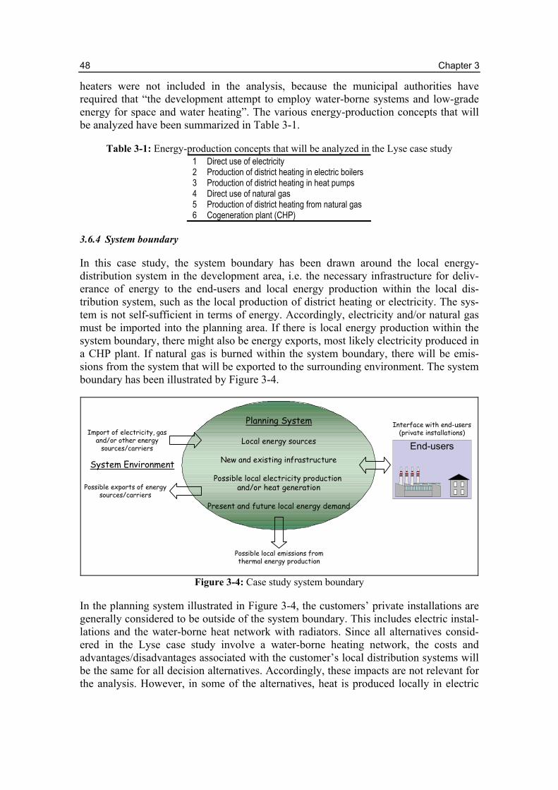
It is important to spend sufficient time and resources on the problem definition and structuring, so that all disagreements among the decision-maker(s) (DM(s)) and the analyst regarding the nature of the problem and the desired goals are eliminated. After the problem has been properly identified, the next step of a multi-criteria energy-planning process is the building of an energy system model (impact model). The model is used to calculate the operational attributes necessary for the multi-criteria analysis; in other words, to determine the various alternatives’ performance values for some or all of the criteria being considered. It is important that the model accounts for both the physi-cal characteristics of the energy system components and the complex relationships between the system parameters. However, it is not propitious to choose/build an energy system model with a greater level of detail than needed to achieve the aims of the plan-ning project.
v
In my PhD research, I have chosen to use the eTransport model as the energy system model. This model is especially designed for planning of local and regional energy systems, where different energy carriers and technologies are considered simultane-ously. However, eTransport can currently provide information only about costs and emissions directly connected to the energy system’s operation. Details about the invest-ment plans’ performance on the remaining criteria must be found from other infor-mation sources. Guidelines should be identified regarding the extent to which different aspects should be accounted for, and on the ways these impacts can be assessed for each investment plan under consideration. However, it is important to realize that there is not one solution for how to do this that is valid for all kind of local energy-planning problems. It is therefore necessary for the DM(s) and the analyst to discuss these issues before entering the decision-making phase.
The Decision-Making Phase
Two case studies have been undertaken to examine to what extent the use of MCDA is suitable for local energy-planning purposes. In the two case studies, two of the most well-known MCDA methods, the Multi-Attribute Utility Theory (MAUT) and the Analytical Hierarchy Process (AHP), have been tested. Other MCDA methods, such as GP or the outranking methods, could also have been applied. However, I chose to focus on value measurement methods as AHP and MAUT, and have not tested other methods. Accordingly, my research cannot determine if value measurement methods are better suited for energy-planning purposes than GP or outranking methods are.
Although all MCDA methods are constructed to help DMs explore their ‘true values’ – which theoretically should be the same regardless of the method used to elicit them – our experiments showed that different MCDA methods do not necessarily provide the same results. Some of the differences are caused by the two methods’ different ways of asking questions, as well as the DMs’ inability to express clearly their value judgements by using one or both the methods. In particular, the MAUT preference-elicitation proce-dure was difficult to understand and accept for DMs without previous experience with the utility concept. An additional explanation of the differences is that the external uncertainties included in the problem formulation are better accounted for in MAUT than in AHP. There are also a number of essential weaknesses in the theoretical foun-dation of the AHP method that may have influenced the results using that method. How-ever, the AHP method seems to be preferred by DMs, because the method is straight-forward and easier to use and understand than the relatively complex MAUT method.
It was found that the post-interview process is essential for a good decision outcome. For example, the results from the preference aggregation may indicate that according to the DM’s preferences, a modification of one of the alternatives might be propitious. In such cases, it is important to realize that MCDA is an iterative process. The post-interview process also includes presentation and discussion of results with the DMs. Our experiments showed that the DMs might discover inconsistencies in the results; that the results do not reflect the DM’s actual preferences for some reason; or that the results simply do not feel right. In these cases, it is again essential to return to an earlier phase of the MCDA process and conduct a new analysis where these problems or discrepan-cies are taken into account.
vi
The results from an MAUT analysis are usually presented to the DMs in the form of expected total utilities given on a scale from zero to one. Expected utilities are conven-ient for ranking and evaluation of alternatives. However, they do not have any direct physical meaning, which quite obviously is a disadvantage from an application point of view. In order to improve the understanding of the differences between the alternatives, the Equivalent Attribute Technique (EAT) can be applied. EAT was tested in the first of the two case studies. In this case study, the cost criterion was considered important by the DMs, and the utility differences were therefore converted to equivalent cost differ-ences. In the second case study, the preference elicitation interviews showed, quite sur-prisingly, that cost was not considered among the most important criteria by the DMs, and none of the other attributes were suitable to be used as the equivalent attribute. Therefore, in this case study, the use of EAT could not help the DMs interpreting the differences between the alternatives.
Summarizing
For MCDA to be really useful for actual local energy planning, it is necessary to find/design an MCDA method which: (1) is easy to use and has a transparent logic; (2) presents results in a way easily understandable for the DM; (3) is able to elicit and aggregate the DMs' real preferences; and (4) can handle external uncertainties in a con-sistent way.
Thesis outline
The thesis consists of four parts, which are organized as follows:
• ‘Introduction’, which introduces energy-system planning (Chapter 1) and the con-cept of multi-criteria decision analysis (MCDA) (Chapter 2).
• ‘Problem Structuring and Model-Building Issues’, which discusses the initial phases of a local energy-planning MCDA process, namely the problem identification and problem structuring (Chapter 3); the energy systems model building and input data collection (Chapter 4); and the impact assessment (Chapter 5).
• ‘Preference Elicitation and Aggregation in the MCDA Process’, which experimen-tally compares the use of two MCDA methods, and discusses their advantages and drawbacks (Chapter 6); compares how the two MCDA methods can be used to assist in decision making under uncertainty (Chapter 7); presents the equivalent attribute method (EAT), and discusses how EAT can be used to improve the comprehensi-bility of a MCDA study (Chapter 8); and discusses the importance of the interaction between the DMs and the analyst during the MCDA process (Chapter 9). The dis-cussions are based on two local energy-planning case studies.
• ‘Discussion, Conclusion and Suggestions for Further Research’, which discusses the findings and results, and presents the main conclusions of my PhD study. In the end, it is given some suggestions for future areas of research.
vii
Contributions
The main objective of this doctoral project has been to propose how a multi-criteria based approach can be applied to discrete investment planning in local energy systems with multiple energy carriers. The proposal is based on two experimental case studies.
The contributions of the thesis can be summarized as follows:
• A requirement specification for an MCDA based planning framework, including the elements:
- Easy to use with transparent logic - Results presented in a way easily understood by DMs - Able to elicit and aggregate the DMs’ preferences consistently - Consistent handling of uncertainties
• A description of a planning framework with the main elements:
- Identification and structuring of the problem - Building of impact model(s) (energy system model) - Impact assessment - Preference elicitation and aggregation (preference model building) - Decision-making/development of an action plan - Implementation of the decision
• Experimental testing of two MCDA methods (MAUT and AHP) on a local energy-planning problem, with emphasis on comparison of the methods based on the requirement specification described above.
• Demonstration and evaluation of the Equivalent Attribute Technique (EAT) as an instrument to compare alternatives by converting total preference values for the alternatives into equivalent differences in one of the decision criteria, preferably an economic criterion. EAT, as it is used in this thesis, is an elaboration of an idea used by Keeney and his co-workers.
• Providing case based experience that clearly demonstrates the importance of the interaction between the DM(s) and the analyst, specifically the elements:
- Problem structuring and identification - Selection of criteria and attributes - The use of proxy criteria - Interpretation of results
viii
Table of Contents
PREFACE.................................................................................................................................................... i
ACKNOWLEDGEMENTS ............................................................................................................................. ii
ABSTRACT ............................................................................................................................................... iv
BACKGROUND AND MOTIVATION............................................................................................................ iv THE INITIAL STRUCTURING AND MODELLING PHASE.............................................................................. iv THE DECISION-MAKING PHASE................................................................................................................ v SUMMARIZING.........................................................................................................................................vi THESIS OUTLINE ......................................................................................................................................vi
PART A: INTRODUCTION ..........................................................................................1 SOME IMPORTANT CONCEPTS ...................................................................................................... 3 ENERGY SYSTEMS AND ENERGY-SYSTEM PLANNING.................................................................. 3 MCDA......................................................................................................................................... 3
1. ENERGY SYSTEMS AND ENERGY-SYSTEM PLANNING .................................................... 5
1.1 ENERGY SYSTEMS ........................................................................................................................ 5 1.2 ENERGY-SYSTEM PLANNING........................................................................................................ 7 1.3 REFERENCES ................................................................................................................................ 9
2. MULTI-CRITERIA DECISION ANALYSIS IN LOCAL ENERGY PLANNING ................. 11
2.1 WHAT IS MCDA?....................................................................................................................... 11 2.2 A COMPARISON BETWEEN MCDA AND CBA ............................................................................ 12 2.3 CLASSIFYING MCDA METHODS ................................................................................................ 15 2.3.1 Value-measurement methods ............................................................................................... 16 2.3.2 Goal, aspiration and reference-level methods ..................................................................... 18 2.3.3 Outranking methods............................................................................................................. 19 2.4 CHOOSING AN MCDA METHOD................................................................................................. 20 2.5 MCDA AND ENERGY PLANNING – A REVIEW............................................................................ 21 2.5.1 Value-measurement methods ............................................................................................... 21 2.5.2 Goal, aspiration and reference-level methods ..................................................................... 22 2.5.3 Outranking methods............................................................................................................. 22 2.5.4 Combination of methods ...................................................................................................... 23 2.6 MCDA AND PLANNING OF LOCAL ENERGY SYSTEMS WITH MULTIPLE ENERGY CARRIERS ...... 24 2.7 REFERENCES .............................................................................................................................. 24
ix
PART B: PROBLEM STRUCTURING AND MODEL-BUILDING ISSUES .......31 THE MULTI-CRITERION DECISION ANALYSIS (MCDA) PROCESS .............................................. 33 THE INITIAL STRUCTURING AND MODELLING PHASE................................................................. 34 REFERENCES .............................................................................................................................. 34
3. PROBLEM IDENTIFICATION AND PROBLEM STRUCTURING ...................................... 35
3.1 STAKEHOLDER ANALYSIS .......................................................................................................... 35 3.1.1 The Energy Company and Internal Stakeholders ................................................................ 36 3.1.2 Development/construction companies ................................................................................. 37 3.1.3 The end-users/customers...................................................................................................... 37 3.1.4 Regulators and National/Local Authorities ......................................................................... 38 3.1.5 Other companies .................................................................................................................. 39 3.1.6 Third party ........................................................................................................................... 39 3.2 SYSTEMS AND SYSTEM BOUNDARIES ......................................................................................... 40 3.2.1 Decomposition of energy systems ........................................................................................ 41 3.3 OBJECTIVES AND CRITERIA IN ENERGY-SYSTEMS PLANNING .................................................... 43 3.4 DECISION ALTERNATIVES .......................................................................................................... 44 3.5 MAIN UNCERTAINTIES ............................................................................................................... 44 3.6 LYSE CASE STUDY ..................................................................................................................... 46 3.6.1 Premises for the planning problem ...................................................................................... 46 3.6.2 Stakeholders and objectives in the case study...................................................................... 47 3.6.3 Investment alternatives ........................................................................................................ 47 3.6.4 System boundary .................................................................................................................. 48 3.7 REFERENCES .............................................................................................................................. 49
4. ENERGY SYSTEMS MODEL BUILDING AND INPUT DATA COLLECTION.................. 51
4.1 ENERGY MODELLING ................................................................................................................. 51 4.2 THE ETRANSPORT MODEL.......................................................................................................... 52 4.2.1 Modelling in the eTransport model...................................................................................... 52 4.2.2 eTransport investment model ............................................................................................... 54 4.2.3 eTransport advantages/disadvantages for multi-criteria analyses of local energy systems 55 4.3 LYSE CASE STUDY IN THE ETRANSPORT MODEL........................................................................ 56 4.4 MODEL ATTRIBUTES AND UNCERTAINTIES ................................................................................ 58 4.4.1 Energy-demand forecast ...................................................................................................... 59 4.4.2 Electricity and gas price ...................................................................................................... 62 4.4.3 Discounting and discount rate ............................................................................................. 65 4.5 REFERENCES .............................................................................................................................. 66
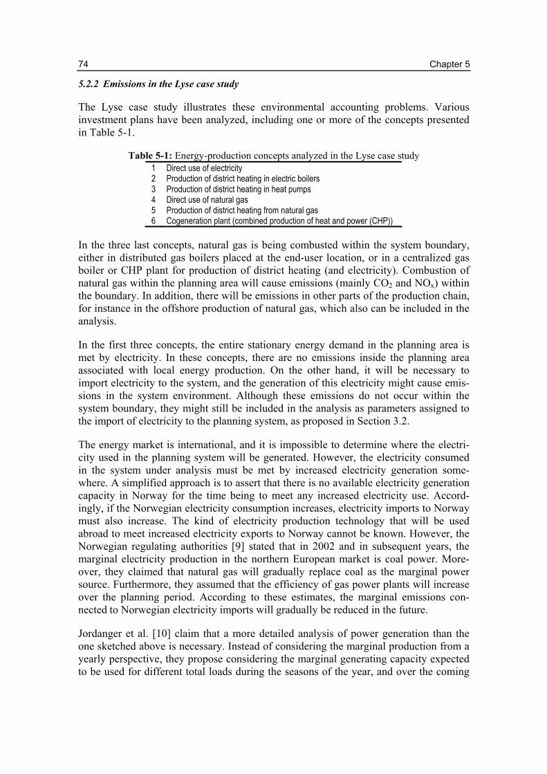
5.1 ECONOMIC CRITERIA.................................................................................................................. 69 5.1.1 Socio-economic approach.................................................................................................... 69 5.1.2 Energy transportation .......................................................................................................... 70 5.2 ENVIRONMENTAL CRITERIA....................................................................................................... 73 5.2.1 Environment and system boundaries ................................................................................... 73 5.2.2 Emissions in the Lyse case study.......................................................................................... 74 5.2.3 Energy resource utilization.................................................................................................. 75 5.2.4 Other environmental effects ................................................................................................. 77 5.3 OTHER CRITERIA........................................................................................................................ 77 5.4 REFERENCES .............................................................................................................................. 78
x
PART C: PREFERENCE ELICITATION AND AGGREGATION IN THE MCDA PROCESS – TWO CASE STUDIES.............................................81
MCDA IN LOCAL ENERGY PLANNING ....................................................................................... 83 THE DECISION-MAKING PHASE IN THE MCDA PROCESS........................................................... 83 GROUP DECISIONS...................................................................................................................... 83 SUMMARY OF CHAPTERS 6-9...................................................................................................... 84 REFERENCES .............................................................................................................................. 85
6. PLANNING OF MIXED LOCAL ENERGY-DISTRIBUTION SYSTEMS: A COMPARISON OF TWO MULTI-CRITERIA DECISION METHODS ............................ 87
6.1 INTRODUCTION........................................................................................................................... 87 6.2 A FRAMEWORK FOR LOCAL ENERGY-SYSTEM PLANNING ......................................................... 88 6.2.1 An integrated planning approach ........................................................................................ 88 6.2.2 The impact model................................................................................................................. 89 6.2.3 The preference models ......................................................................................................... 90 6.3 THE CASE STUDY ....................................................................................................................... 92 6.3.1 Criteria, alternatives, scenarios and impact model results.................................................. 92 6.3.2 Preference elicitation........................................................................................................... 95 6.4 RESULTS..................................................................................................................................... 97 6.4.1 Comparison of results from the MAUT and AHP experiments ............................................ 97 6.4.2 Preferences of DM A............................................................................................................ 99 6.4.2 Preferences of DM C ......................................................................................................... 100 6.5 EVALUATION AND COMPARISON OF METHODS ........................................................................ 101 6.5.1 Internal uncertainties......................................................................................................... 101 6.5.2 External uncertainties ........................................................................................................ 102 6.5.3 The theoretical foundation of AHP .................................................................................... 102 6.5.4 MAUT complexity .............................................................................................................. 105 6.5.5 Other advantages and drawbacks of the two methods ....................................................... 106 6.6 CONCLUSIONS .......................................................................................................................... 106 6.7 ACKNOWLEDGEMENTS............................................................................................................. 107 6.8 REFERENCES ............................................................................................................................ 107
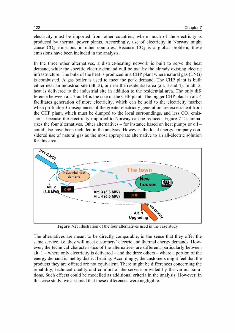
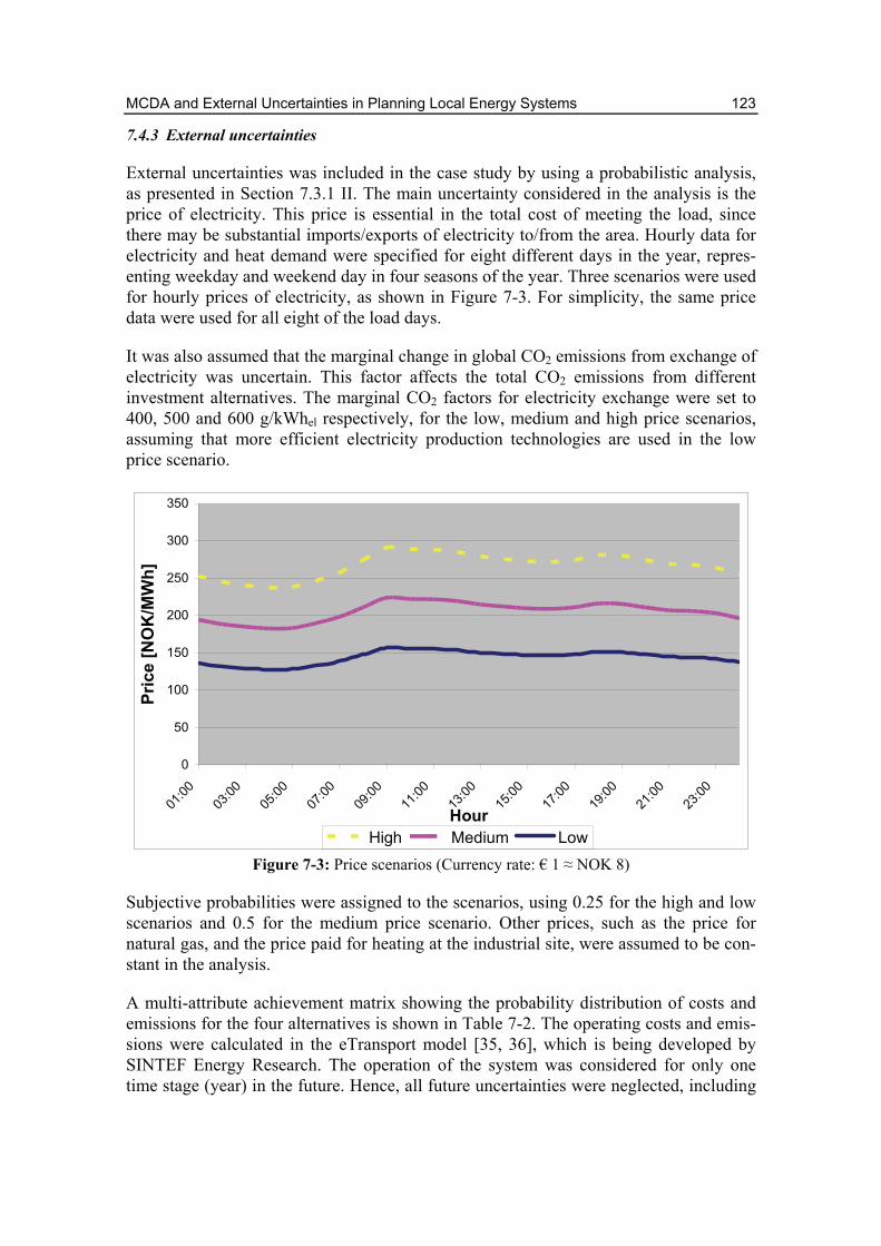
7. MCDA AND EXTERNAL UNCERTAINTIES IN PLANNING LOCAL ENERGY SYSTEMS..................................................................................................... 111
8. USE OF THE EQUIVALENT ATTRIBUTE TECHNIQUE IN MULTI-CRITERIA PLANNING OF LOCAL ENERGY SYSTEMS .................................... 131
8.1 INTRODUCTION......................................................................................................................... 131 8.2 THE MULTI-ATTRIBUTE UTILITY THEORY (MAUT) ................................................................ 131 8.3 THE EQUIVALENT ATTRIBUTE TECHNIQUE (EAT) ................................................................... 133 8.3.1 Motivation .......................................................................................................................... 133 8.3.2 Description of EAT ............................................................................................................ 133 8.3.3 Comparison between the Equivalent Attribute Technique and Cost-Benefit Analysis....... 135 8.4 A LOCAL ENERGY-PLANNING PROBLEM AND THE USE OF MAUT .......................................... 136 8.4.1 Criteria, alternatives and uncertainties in the case study.................................................. 137 8.4.2 Calculation of costs and other criteria .............................................................................. 138 8.4.3 Performance values and preference elicitation ................................................................. 139 8.5 EAT APPLIED TO THE CASE STUDY ......................................................................................... 139 8.5.1 Simplified, linear EAT model ............................................................................................. 140 8.5.2 Advanced, non-linear EAT model ...................................................................................... 142 8.6 CONCLUSIONS .......................................................................................................................... 145 8.7 ACKNOWLEDGEMENTS............................................................................................................. 145 8.8 REFERENCES ............................................................................................................................ 146 APPENDIX................................................................................................................................. 148
9. VALUE AND PREFERENCE MODELLING IN THE LYSE CASE STUDY....................... 151
9.1 INTERACTION BETWEEN THE DM(S) AND THE ANALYST IN AN MCDA PROCESS .................... 151 9.2 THE PRE-INTERVIEW DISCUSSION AND IMPACT MODELLING................................................... 152 9.2.1 The criteria in the case studies .......................................................................................... 152 9.2.2 Choice of attributes............................................................................................................ 155 9.2.3 The investment plans and impact model results................................................................. 156 9.3 THE PREFERENCE-ELICITATION INTERVIEWS........................................................................... 157 9.3.1 Preferences of participant A .............................................................................................. 158 9.3.2 Preferences of participant B .............................................................................................. 159 9.3.3 Preferences of participant C .............................................................................................. 160 9.3.4 Additional investment plan ................................................................................................ 161 9.4 POST-INTERVIEW DISCUSSIONS AND DIFFICULTIES IN THE PREFERENCE-ELICITATION
INTERVIEWS ............................................................................................................................. 162 9.4.1 Insight into the criteria and understanding of MAUT........................................................ 163 9.4.2 Low weighting of economic criterion................................................................................. 164 9.4.3 Trade-off questions ............................................................................................................ 165 9.4.4 Use of the Equivalent Attribute Technique ........................................................................ 166 9.5 CONCLUSIONS FROM THE LYSE CASE STUDY .......................................................................... 167 9.6 REFERENCES ............................................................................................................................ 168
PART D: DISCUSSION, CONCLUSION AND SUGGESTIONS FOR FURTHER RESEARCH ...........................................................................169
DISCUSSION.............................................................................................................................. 171 The theory of MCDA and local energy planning ............................................................... 171 MCDA in realistic applications ......................................................................................... 171 Problem structuring and selection of criteria and attributes............................................. 172 Different methods and comparison of results .................................................................... 172 Choice of MCDA method ................................................................................................... 173 CONCLUSIONS .......................................................................................................................... 174 SUGGESTIONS FOR FURTHER RESEARCH.................................................................................. 176
xii
Definitions and Abbreviations
MCDA: Multi-Criteria Decision Analysis. The use of methods that help people make decisions according to their preferences in cases characterized by multiple conflicting criteria [3]. See Section 2.1 for more details.
Decision-maker (DM): The person or entity that is responsible for making a decision. The DM might be an individual, a small, homogenous group with common goals, a large group representing different elements of an organization, or a number of highly diverse interest groups [4].
Stakeholder: Everybody who has a legitimate interest in the system, or “those who have a right to impose requirements on a solution”. An alternative definition is those who “have demonstrated their need or willingness to be involved in seeking a solution” [5]. See Section 3.1 for more details.
Analyst: The person who models the situation under study, assists the DM in reaching a satisfactory decision, and makes recommendations for the final choice. The analyst should not express any personal preferences, but should facilitate the elicitation of DM’s preferences, which should be treated as objectively as possible [4, 6].
Alternative: Projects, candidates, and investment plans, among which a choice has to be made [6]. The term is often used for actions that are mutually exclusive in terms of implementation [7]. There can either be a finite number of explicitly defined discrete alternatives or implicitly defined continuous alternatives.
Optimal/ideal alternative: An alternative that results in the maximum performance value for each of the objective functions simultaneously [8]. An ideal alternative will very seldom be found in the real world.
Dominance: If – in a pairwise comparison of two alternatives – an alternative A scores higher than alternative B on at least one criterion and does not score lower on any of the other criteria, then A dominates B, while B is dominated by A.
Objective: An objective is a statement of something that one wants to achieve and is characterized by a decision context, an object and a direction of preference [9]. Broad overall objectives, or ultimate objectives, are broken into lower-level or inter-mediate objectives that are more concrete, and these may be further detailed as sub-objectives, immediate objectives, or criteria that are more operational [10].
Example: Minimize impacts on global climate from greenhouse gas emissions.
Criterion: A tool constructed for the evaluation and comparison of alternatives and the degree to which they achieve objectives. The criteria offer comprehensive and measur-able representations of the DM’s preferences [7, 10, 11].
Example: Emissions of CO2 during the lifetime of the investment.
xiii
Quantitative criterion: A criterion that can be measured on a clear, concrete defined scale.
Qualitative criterion: A criterion for which evaluations cannot be made on a numerical basis [6]. Instead, a verbal scale or an ordinal ranking can be used.
Attribute: A quantitative measure of performance, used to evaluate directly or indirectly the degree to which the objectives are achieved [4, 12]. A good attribute both defines precisely what the associated objective means and serves as a scale to describe the con-sequences of the alternative [13].
Example: Tonnes of CO2 emissions.
Natural attribute: A property that directly measures the extent to which an objective is met. A natural attribute can be counted or physically measured, is in general use and has a common interpretation [14].
Proxy attribute: Proxy attributes do not directly measure the objective of concern, and are used if it is difficult to find a natural attribute for a criterion. A proxy attribute is an attribute that captures most of the idea in the objective, and involve a scale that can be counted or measured and is in common use [2, 14].
Performance value (PV): A measure of how well an alternative performs for a given attribute.
Criteria weight: Assessment of the relative importance of a given criterion [11]. The weight of a criterion can reflect both the range of difference of the options and how much that difference matters.
AHP: Analytical Hierarchy Process. Another well-known MCDA method. Explained and exemplified in Chapter 6. See also [15] for a detailed description of the method.
MAUT: Multi-Attribute Utility Theory. A well-known MCDA methods. Explained and exemplified in Chapter 6. See also [16] for a detailed description of the method.
Utility: An expression of the DM’s overall valuation of an option in terms of the value of its performance on each of the separate criteria [10].
Utility function: A preference representation function under risk [17].
References
[1] S. Johansen: Energy Resource Planning: A Conceptual Study of a Multiobjective Problem, Doktor Ingeniør Avhandling 1992:6, Trondheim: The University of Trondheim, The Norwegian Institute of Technology, Division of Electrical Power Engineering, 1992.
[2] M.D. Catrinu: Decision Aid for Planning Local Energy Systems: Application of Multi-Criteria Decision Analysis, Doctoral Theses 2006:62, Trondheim: Norwegian University of Science and Technology, Faculty of Information Technology, Mathematics and Electrical Engineering, Department of Electrical Power Engineering, 2006.
xiv
[3] P. Bogetoft and P.M. Pruzan: Planning with Multiple Criteria: Investigation, Communication and Choice, København: Handelshøjskolens forlag, 1997.
[4] V. Belton and T.J. Stewart: Multiple Criteria Decision Analysis: An Integrated Approach, Boston: Kluwer Academic Publications, 2002.
[5] N. Sproles: "Coming to Grips with Measures of Effectiveness", Systems Engineering, vol. 3 (1), p. 50-58, 2000.
[6] J.-C. Pomerol and S. Barba-Romero: Multicriterion Decision in Management: Principles and Practice, Boston: Kluwer Academic Publishers, 2000.
[7] B. Roy: "Paradigms and Challenges", in J. Figueira, S. Greco, and M. Ehrgott (Eds.): Multiple Criteria Decision Analysis: State of the Art Surveys. New York: Springer, p. 3-24, 2005.
[8] C.-L. Hwang and K. Yoon: Multiple Attribute Decision Making: Methods and Applications: A State-of-the-Art Survey, Berlin: Springer, 1981.
[9] R.L. Keeney and T.L. McDaniels: "Value-Focused Thinking About Strategic Decisions at BC Hydro", Interfaces, vol. 22 (6), p. 94-109, 1992.
[10] J. Dodgson, M. Spackman, A. Pearman, and L. Phillips: DTLR Multi-Criteria Analysis Manual, UK Dept. for Transport, Local Government and the Regions, 2001. Available from Internet: http://www.communities.gov.uk/pub/252/MulticriteriaanalysismanualPDF1380Kb_id1142252.pdf.
[11] V. Belton and J. Pictet: "A Framework for Group Decision using a MCDA Model: Sharing, Aggregating or Comparing Individual Information", Journal of Decision Systems, vol. 6 (3), p. 283-303, 1997.
[12] R.L. Keeney: Siting Energy Facilities, New York: Academic Press, 1980.
[13] R.L. Keeney and T.L. McDaniels: "Identifying and Structuring Values to Guide Integrated Resource Planning at BC Gas", Operations Research, vol. 47 (5), p. 651-662, 1999.
[14] R.L. Keeney and R.S. Gregory: "Selecting Attributes to Measure the Achievement of Objectives", Operations Research, vol. 53 (1), p. 1-11, 2005.
[15] T.L. Saaty: The Analytic Hierarchy Process: Planning, Priority Setting, Resource Allocation, New York: McGraw-Hill, 1980.
[16] R.L. Keeney and H. Raiffa: Decisions with Multiple Objectives: Preferences and Value Tradeoffs, Cambridge: Cambridge University Press, 1993.
[17] J.S. Dyer: "MAUT - Multiattribute Utility Theory", in J. Figueira, S. Greco, and M. Ehrgott (Eds.): Multiple Criteria Decision Analysis: State of the Art Surveys. New York: Springer, p. 265-295, 2005.
“Nothing is more difficult, and therefore more precious, than to be able to decide.”
Napoleon, Maxims, 1804
“Experience is a good teacher, but she sends in terrible bills.”
Minna Thomas Antrim
"There is always an easy solution to every human problem – neat, plausible, and wrong."
Henry Louis Mencken, The Divine Afflatus, New York Evening Mail, 1917
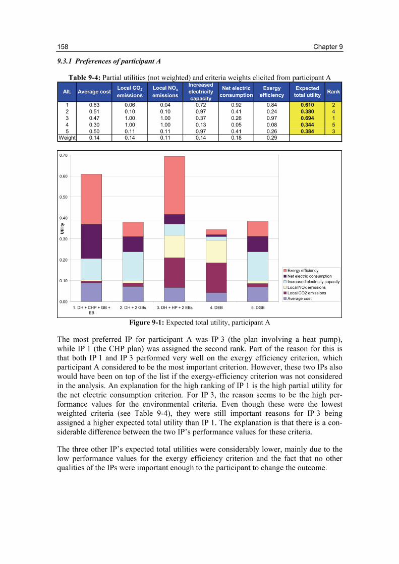
2 Part A
Part A 3
Some Important Concepts
The title of this thesis is multi-criteria planning of local energy systems with multiple energy carriers. Part A of the thesis will introduce and explain the concepts of ‘local energy systems’, ‘energy-system planning’ and ‘Multi-Criteria Decision Analysis’.
Energy Systems and Energy-System Planning
Chapter 1 will give a brief overview of the Norwegian energy infrastructure during the last decades. Combined energy systems where several energy carriers can be delivered to the customers have been more common during this period. In the past, different infra-structures were normally planned and commissioned by independent companies. How-ever, it is believed that synergetic effects might be lost when such infrastructures are planned independently. Consequently, planning tools that can evaluate and analyze alternative energy carriers in mutual combination will give some benefits.
MCDA
Multi-Criteria Decision Analysis (MCDA) is an umbrella term for methods that can help decision-makers to make decisions according to their preferences in cases where there are more than one conflicting criterion. Chapter 2 begins with an explanation of the MCDA concept, and compares MCDA with the more traditional cost-benefit analysis concept. Thereafter, some of most well-known and mostly used MCDA methods are presented, with an evaluation of the main advantages and drawbacks of the different methods, and guidelines for the selection of the most appropriate method for a given problem. The chapter concludes with a brief review of MCDA analyses that has been conducted in the energy-planning sector, and some basic ideas on how MCDA can be used for planning of local energy systems with multiple energy carriers.
4 Part A
5
1. Energy Systems and Energy-Systems Planning 1.1 Energy Systems
The term “energy system” is used in a variety of scientific settings and contexts, and it is difficult to find a common definition of the term. This thesis will use the term “energy system” to refer to energy-distribution systems, i.e. systems used to supply society with continuous access to necessary energy services. Accordingly, energy systems are inter-connected infrastructures that “combine the sources of energy, the means for converting these sources to usable forms, the distribution devices and procedures, the using community and the ways it employs energy, and the surrounding natural and economic environment” [1, p. 161]. This definition includes both the technical and the economic side of the energy infrastructure. It is important to realize that no one actually needs energy in and of itself. However, energy is necessary to provide a number of important services in society, such as heating, lighting, mechanical work, entertainment etc., both in the industrial, commercial and residential sectors.
Norway has traditionally met most of its stationary energy demand (including heating) with electricity, because of abundant access to cheap hydropower. However, during the 1990s, the Norwegian electricity sector was decentralized and liberalized. This led to many important changes, such as changes in energy-sector ownership and responsibili-ties [2]. Before liberalization, each energy company was required to have sufficient power generation capacity to supply electricity to every customer in their service area. This resulted in substantial over-capacity in the Norwegian market as a whole. As a result of liberalization, energy companies no longer have power capacity responsibili-ties. Instead, market mechanisms are supposed to ensure that the total power generation capacity of the Nordic market is sufficient to meet the demand while at the same time avoiding over-capacity. This goal has not been entirely met. After deregulation, the increase in electricity demand has been much higher than the increase in generation capacity. The result is that Norway’s electricity generation capacity no longer is suffi-cient to meet demand, and accordingly, Norway is at present (in normal hydrological years) a net importer of electricity.
The under-capacity in electricity generation capacity has led to an increased focus on alternative energy solutions. District heating (DH) networks are being built in many areas. In other areas, there are companies offering natural gas, either through a gas network, or in bulk. This thesis will focus on energy systems in such areas, which are commonly called “combined energy-distribution systems”, as illustrated in Figure 1-1. In this context, the term implies energy systems with a mix of distributed energy sources, end uses and infrastructures for several energy carriers in the same area.
An energy carrier can be defined as “any system or substance that contains energy for conversion as usable energy later or somewhere else” [3]. The energy carriers in a typi-cal energy system can be divided in two groups; (1) energy carriers delivered in bulk by vehicles (for instance tankers), e.g. oil and firewood, and (2) energy carriers normally delivered through cables or pipelines, e.g. electricity, DH, natural gas, and in the future, possibly hydrogen. This thesis will focus solely on the second group of energy carriers, illustrated by the ovals in Figure 1-1.
6 Chapter 1
Industry
Natural gas/Hydrogen
Natural gas/Hydrogen
photovoltaicwind
hydro
ElectricityElectricity
sun heat biomass
District heatingDistrict heatingwaste heat
National andregionalenergy
systems
National andregionalenergy
systems
biomass coaloil
gasoilBuildings
Industry
Natural gas/Hydrogen
Natural gas/Hydrogen
photovoltaicwind
hydro
ElectricityElectricity
sun heat biomass
District heatingDistrict heatingwaste heat
National andregionalenergy
systems
National andregionalenergy
systems
biomass coaloil
gasoilBuildings
Figure 1-1: A combined energy-distribution system
It is important to realize that not all energy carriers can be used to meet all energy demands. Various energy carriers and energy sources have different physical character-istics that affect their usefulness and quality [4]. For instance, DH is just hot water in pipes. Hot water is very well suited for space heating and water heating, but it is not useful for many other purposes. Accordingly, it is considered a low-quality energy car-rier. Electricity, on the other hand, is extremely flexible, and is accordingly a high-quality energy carrier. Electricity can be used for heating purposes. However, it can also be used for almost all other energy purposes, from lighting, to powering home appli-ances, to driving motors and machines. Because electricity is so flexible, it is common practice to burn lower-quality energy carriers such as gas, oil, and coal, in power plants to produce electricity, even though a great deal of the energy content is lost in the con-version. When we build combined energy systems, we can make use of the synergistic effects in such systems. For instance, in combined systems, there may be an advantage in avoiding the use of electricity for low-quality energy demands like heating. It is often better to use low-quality energy carriers, like DH and natural gas, for heating purposes. The result is a much more efficient energy system.
The supply side of a local energy system can consist of both local and imported energy resources. Some energy resources, such as natural gas, can be used directly at the end-user location. Other resources must be converted into electricity or DH to be useful for the end-user. The development of new technologies for distributed generation has trans-formed some of the traditional end-users in the system (mainly industrial customers) into suppliers of electricity or heat. At the demand side of the system, the energy meets a number of important services in society, such as heating, lighting, and mechanical work, both in the industrial and residential sectors.
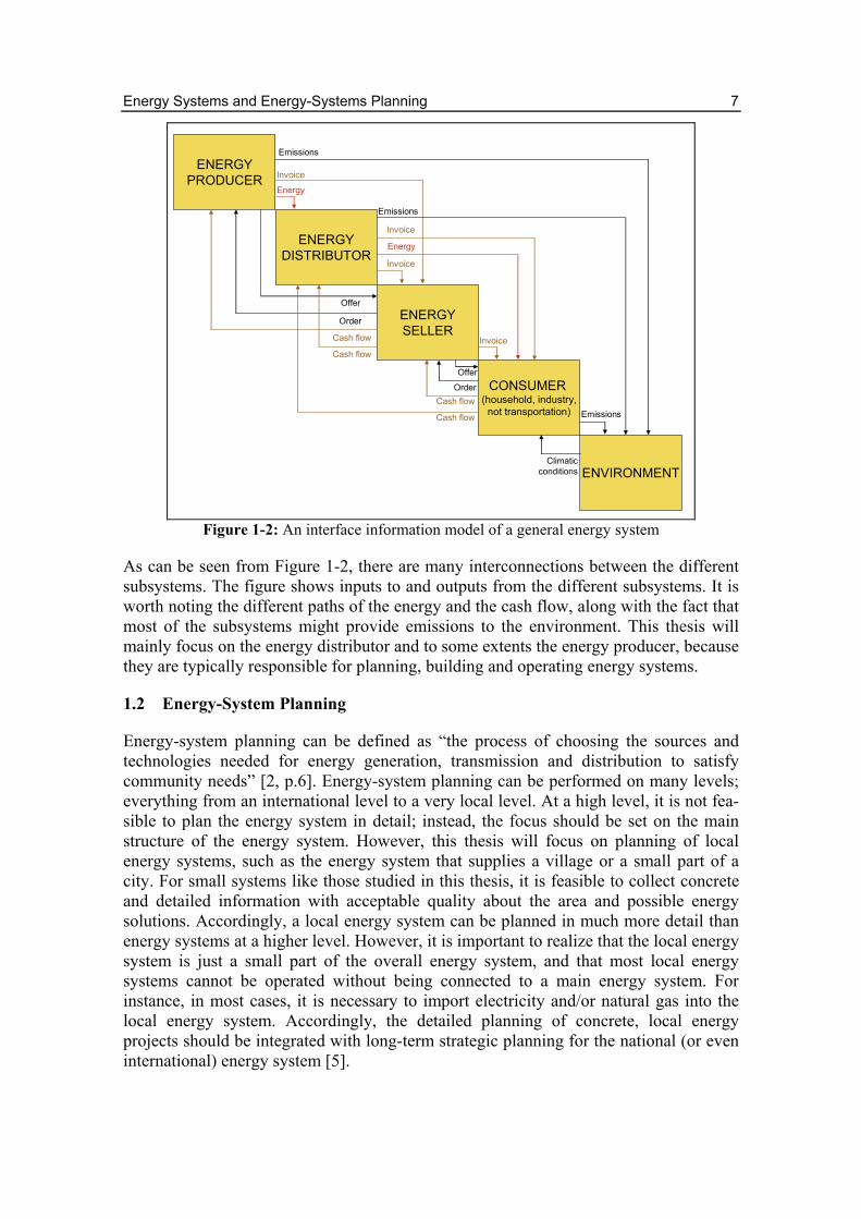
Figure 1-2 shows an interface information model of a complete energy system. An energy system can be divided in five subsystems; the producer, the distributor, the seller, the consumer and the environment. Even though the producer, distributor and seller are often part of the same company, or subsidiaries within the same corporation, they can also be separate companies.
Energy Systems and Energy-Systems Planning 7
ENERGYPRODUCER
ENERGYDISTRIBUTOR
ENERGYSELLER
CONSUMER (household, industry,
not transportation)
ENVIRONMENT
Energy
Energy
Offer
Offer
Order
Order
Invoice
Invoice
Invoice
Climatic conditions
Cash flow
Cash flow
Cash flow
Invoice
Cash flow
Emissions
Emissions
Emissions
Figure 1-2: An interface information model of a general energy system
As can be seen from Figure 1-2, there are many interconnections between the different subsystems. The figure shows inputs to and outputs from the different subsystems. It is worth noting the different paths of the energy and the cash flow, along with the fact that most of the subsystems might provide emissions to the environment. This thesis will mainly focus on the energy distributor and to some extents the energy producer, because they are typically responsible for planning, building and operating energy systems.
1.2 Energy-System Planning
Energy-system planning can be defined as “the process of choosing the sources and technologies needed for energy generation, transmission and distribution to satisfy community needs” [2, p.6]. Energy-system planning can be performed on many levels; everything from an international level to a very local level. At a high level, it is not fea-sible to plan the energy system in detail; instead, the focus should be set on the main structure of the energy system. However, this thesis will focus on planning of local energy systems, such as the energy system that supplies a village or a small part of a city. For small systems like those studied in this thesis, it is feasible to collect concrete and detailed information with acceptable quality about the area and possible energy solutions. Accordingly, a local energy system can be planned in much more detail than energy systems at a higher level. However, it is important to realize that the local energy system is just a small part of the overall energy system, and that most local energy systems cannot be operated without being connected to a main energy system. For instance, in most cases, it is necessary to import electricity and/or natural gas into the local energy system. Accordingly, the detailed planning of concrete, local energy projects should be integrated with long-term strategic planning for the national (or even international) energy system [5].
8 Chapter 1
Before the 1970s, there was little effort to formally plan energy systems. The oil crisis in the 1970s resulted in more emphasis on identifying efficient supply options. It has been common for different energy infrastructures – such as electricity, DH and natural gas networks – to have been planned and commissioned by independent companies. Since energy distribution through networks is a natural monopoly, distribution compa-nies in most cases do not need to worry about competition from other investors. How-ever, if different distribution companies are in charge of different energy networks in the same area, there will be competition between the energy carriers in meeting the energy needs of end-users. The various energy companies do not necessarily share the same objectives, however. In Norway, electricity network companies are, from a socio-economic point of view, required by law to provide reliable service to any customer in their service area. From business point of view, they seek to provide their service as profitably as possible. Independent companies that build other energy networks make decisions based solely on business economics. They will in general establish themselves in an area only if they think they can make a profit. A system like this, however, means that the synergistic effects in a combined energy system are to a large extent neglected. Accordingly, there is no guarantee that the energy supply to a certain area will be opti-mal.
In recent years, there has been a shift in the organization and responsibilities of energy companies. Accordingly, local energy planners have been confronted with new chal-lenges. In the short term, the biggest challenge has been to understand the complexity added to the decision-making process by the restructuring of the energy sector and the development of different energy markets. In addition, environmental problems and the continuous depletion of primary resources have added new dimensions to the planning problem in the medium and long term. Consequently, there is a need for new planning methodologies and tools in order to propose solutions both for the short, medium and long term.
In Norway, electricity companies are given extended responsibilities, including the con-sideration of alternative energy carriers to electricity when planning energy supply to new areas. As a consequence, many energy companies now offer several energy ser-vices to their customers. This is in accordance with national goals regarding the deve-lopment of a supplemental energy supply to the hydroelectric system [6]. These changes have led to a need for a more comprehensive and sophisticated energy-planning process, where the various energy infrastructures are planned in a coordinated way. Such inte-grated planning ensures that the synergistic effects in a combined energy system can be taken into account. If different companies are responsible for the various energy infra-structures, coordinated planning is more difficult, as each company is only concerned with optimizing the operation and investments in its own distribution network. Invest-ments and other changes in the competitors’ distribution networks will be an uncertain variable – not a decision variable – for each decentralized DM.
To sum up: deregulation of the electricity sector and the introduction of other energy carriers to the energy system has made the planning of a formalized and structured local energy system considerably more important than before. The purpose of local energy-system planning is to select an energy system that is able to meet the current and future increase in local energy demand and peak power demand for electricity and heating in
Energy Systems and Energy-Systems Planning 9
an area, in order to maximize the ‘well-being’ of society. However, it is important to be aware that energy planning is not a one-time event, but a continuous process. Although it is common to plan over a long time horizon, there is no rule saying that you cannot change the plan if/when the assumptions for the planning change, as they probably will, since it is not possible to predict the kinds of changes that the future will bring.
1.3 References
[1] H.-M. Groscurth and A. Schweiker: "Contribution of Computer Models to Solving the Energy Problem", Energy Sources, vol. 17 (2), p. 161-177, 1995.
[2] M.D. Catrinu: Decision Aid for Planning Local Energy Systems: Application of Multi-Criteria Decision Analysis, Doctoral Theses 2006:62, Trondheim: Norwegian University of Science and Technology, Faculty of Information Technology, Mathematics and Electrical Engineering, Department of Electrical Power Engineering, 2006.
[3] Wikipedia, Available from Internet: http://en.wikipedia.org.
[4] B.J. Fleay: "Energy Quality and Economic Effectiveness", Australian Green Online. Available from Internet: http://greens.org.au/webarticles/peakoil05/bfleay05c/download.
[5] R. Jank (Ed.): Energy Conservation in Buildings and Community Systems Program: Annex 33: Advanced Local Energy Planning (ALEP): A Guidebook, Bietigheim-Bissingen: Fachinstitut Gebäude Klima, 2000.
[6] Norwegian Ministry of Petroleum and Energy: Report to the Storting No. 29 (1998-99) on Norwegian Energy Policy, [Unofficial translation], 1999. Available from Internet: http://www.regjeringen.no/upload/kilde/oed/rap/2000/0003/ddd/pdfv/115861-eng_oversettelse_kap1_og_2.pdf.
2. Multi-Criteria Decision Analysis in Local Energy Planning 2.1 What is MCDA?
An optimal solution is always the primary goal in decision-making. Unfortunately, a true optimal solution only exists if considering a single criterion. In most real decision situations, basing a decision solely on one criterion is insufficient. Often, it is necessary to plan systems where several conflicting and non-commensurable objectives need to be considered. Especially the cost criterion often comes into conflict with other criteria. This can be called “the eternal problem of limited resources and unlimited needs” [1].
The conventional approach to energy planning is to search for the minimum cost solu-tion that meets both present and future power and energy demands. Other criteria, such as emissions and the reliability of supply, are given monetary values, and included in the cost criteria. Alternatively, they may be considered only as constraints, so that all alternatives that do not meet a minimum/maximum performance target for all other objectives are disregarded [2, 3]. I.e., arbitrary boundary choices are used as substitutes for all but one objective. This classical optimization will provide a solution. However, in many cases the optimization will not provide the “best solution”. The use of con-straints is not particularly helpful in evaluating alternatives, since in reality, there is often more flexibility than is indicated by absolute constraints. For instance, if an alter-native is not able to meet the performance target for one of the more insignificant crite-ria, the alternative will be eliminated, even though the alternative might be among the best for all other criteria. Actually, the use of constraints restricts the most important criterion because the approach guarantees that targets for the less important criteria are first satisfied, before there is any consideration of the criterion considered to be the most important.
New regulations in the energy market – particularly the increased focus on environ-mental impacts from energy systems – have led to more interest in systematic methods for decision aid. A better planning approach is to balance the various criteria, either explicitly or more or less unconsciously, to try to find an acceptable compromise solu-tion. Problem solving that involves complex systems but that does not include the use of any specific methodology might distort the final results. Without the help of tools, decision-makers (DMs) may appear to focus only on a small subset of the criteria, for-mulate their opinions based on insufficient information, or miscalculate with regard to uncertainties [4].
Nevertheless, some authors disagree over the need for advanced decision procedures. Dijksterhuis et al. [5, p. 1005] claim that “it is not always advantageous to engage in thorough conscious deliberation before choosing” and that “choices in complex matters (…) should be left to unconscious thought”. Even though these researchers only inves-tigated choices among consumer products such as cars and furniture, they claimed that they cannot see any a priori reason for their findings not to be valid also for other types of choices. However, this appears to be a major overgeneralization of their research findings, an observation that is also supported by [6] and [7].
12 Chapter 2
‘Multi-criteria decision-making’ (MCDM) is a generic term for the use of methods that help people make decisions according to their preferences, in cases characterized by multiple conflicting criteria [8]. Another term that is frequently used is ‘multi-criteria decision analysis (or ‘decision aid’) (MCDA). The reason for using the second term is to emphasize that the methods themselves cannot make the actual decisions, i.e., they cannot substitute for a DM. The methods’ purpose is to aid DMs in making better decisions by providing good recommendations. There is no strict distinction between the abbreviations MCDM and MCDA. However, MCDA is commonly seen as a more inclusive concept than MCDM [9-11]. MCDA is an extensive process that consists of identification of the problem, problem structuring, preference-model building, use of the model, and determination of an action plan [9, 11]. Accordingly, solving an MCDM problem is just one part – although a very essential part – of the entire MCDA process. In this thesis, the abbreviation MCDA will be used both for the multi-criteria methods and for the entire multi-criteria process.
Ideally, the use of MCDA will help DMs clarify the decision-making process, i.e. to organize and synthesize the information they have collected, so that they can better understand and identify the fundamental criteria in the decision problem. This will make DMs more comfortable with and confident in their decisions, and more able to justify and defend the solution to others. In addition, the use of MCDA often increases discus-sion among stakeholders, activates non-participants, and shifts the focus to the relevant problem issue. The result is often that stakeholders examine the problem comprehen-sively. Accordingly, they will be able to see the problem from other points of views, and they will learn how to recognize and solve conflicts based on misunderstandings. The focus is thus shifted from alternatives to impacts [4]. It can be said that the use of MCDA is a way of dealing with complex problems by breaking them into smaller pieces [12]. After weighing some considerations and making judgements about smaller components, the pieces are reassembled to present an overall picture for the DMs. In this way, choices based on intuition and experience alone can be substituted by a mathe-matical model.
2.2 A Comparison between MCDA and CBA
At present, MCDA is not often used for energy planning in the real world. A more common approach is to apply a cost-benefit analysis (CBA) to a problem. The main principle in CBA is that the performance values for the various criteria are translated into monetary values using commonly agreed-upon conversion factors. The favourable attribute values are summed together as the benefits of the alternative, while the sum of the unfavourable attributes constitutes the cost. The most desirable alternative is the one with the highest net benefit (benefits minus costs). If there are limited funds available, the benefit-to-cost ratio can be used as the decision criterion [13].
As can be seen from the brief presentation of CBA above, there are some mathematical similarities between CBA and many of the MCDA techniques, especially the value-measurement techniques (see Section 2.3.1). Both CBA and MCDA “represent a formalization of common sense for decisions that are too complex for the informal use of common sense” [14, p. 131]. Moreover, both approaches are designed for the identi-fication of the best solution by calculating numbers/scores that reflect the total value of
Multi-Criteria Decision Analysis in Local Energy Planning 13
each of the proposed alternatives. Such similarities should be recognized and possibly used for the benefit of the decision process. However, there are also important differ-ences between the approaches. This section compares the two approaches to call atten-tion to some advantages of MCDA over CBA when it comes to local energy-planning problems.
One important difference between MCDA and CBA is the intellectual roots of the methods [14, 15]. CBA is an older technique, based on the well-developed theory of the welfare economy. Most proponents of CBA are economists, and the main concept of CBA is manipulation of the central substance in economic theory, i.e. money. MCDA, on the other hand, is based on a number of disciplines in addition to economics, such as statistical decision theory, psychology, engineering, systems engineering, operations research and management science. Accordingly, the use of MCDA essentially acknowl-edges that economic efficiency is not the sole objective of policy [16], and that money is not always an accurate measure of value or attractiveness [14].
CBA is a formal procedure based on an objective understanding of reality [15, 17]. The procedure assumes that a constant, linear monetary value/cost can be determined for each of the attributes, based on a collective and scientific view of the importance of the attribute [17]. Since no subjective preferences are supposed to be included in the analy-sis, it is normally not necessary for a CBA analyst to cooperate much with the DM [14]. A CBA is generally limited to those aspects that can be priced in a non-controversial manner. All trade-offs between conflicting goals are supposed to be derived from the marketplace rather than from personal judgements. The use of a monetary scale is advantageous, because such a scale is compatible with market mechanisms and easily understandable by DMs [18]. However, many of the attributes that an energy company might want to include in a local energy-planning analysis have no existing markets. For such attributes, it is difficult to determine objective monetary values. This applies to environmental issues, technical aspects such as reliability and availability, and customer comfort1. The willingness-to-pay principle is normally applied in these cases. However, ordinary people often have no idea about how much they might be willing to pay for things for which there is no existing market. Moreover, they do not want to learn about complex and often hypothetical problems that they face in the valuation of some of the criteria necessary for a CBA analysis. An additional problem is honesty. The people questioned might make a profit from dishonest answers. Even for attributes for which there are markets, it might be difficult to determine an actual socio-economic value. This is due to monopolies, incomplete information, taxes, price subsidies and other political effects [19].
The general idea is that all CBA analysts will make the same value judgments. Accor-dingly, different people performing a CBA for the same problem using the same data are supposed to end up with the same result (at least in the traditional CBA approach) [15], and the results from the CBA can easily be verified by repeating the study. How-
1 However, to some extent there exists a market for some of these issues. For instance, there is established an international CO2 market, and in the Norwegian power system, the power grid companies are economi-cally penalized if they experience any outage time in the power system.
14 Chapter 2
ever, the original idea of everyone ending up with the same result has to some extent been substituted by a more flexible way-of-thinking, and the price used to represent the same criterion (for instance emissions and human life) in various CBA analyses are quite different. Important disadvantages of CBA are that uncertainties and risk attitudes are not directly included2, and that distributional effects (those who receive the benefits are not the same as those who pay the costs) are disregarded [15].
MCDA, on the other hand, lets the DM determine the relative performance of the vari-ous criteria. Accordingly, the use of MCDA provides a representation of the DM’s indi-vidual values, and helps DMs tie conflicting elements together with their personal judgements [15]. This assumes that DMs are willing to reveal their explicit risk prefer-ences and trade-offs, and that the DMs will not, intentionally or unintentionally, mis-interpret their knowledge and preferences to (1) impress the analyst, or (2) to influence the result of the study to their own advantage [14]. Of course, the DM’s judgements may reflect the market prices as long as these prices exist. However, other trade-offs can be chosen if the DM finds that approach to be more relevant, and trade-offs involving attributes where there are no existing markets can be included without necessarily thinking in monetary terms.
MCDA allows trade-offs to be nonlinear if so desired. For instance, the DM can con-sider increased emissions of NOx as less important if existing emissions already are very high than if there are no emissions in the first place. The DMs are also free to include or exclude various aspects from the analysis, based on their own assumptions regarding what is important. To some extent, this is also possible by increasing and decreasing the monetary values of the various aspects in a CBA. However, Watson [15] argues that when decision aid is needed, it is better to use procedures that have been developed particularly for that purpose (i.e. MCDA), instead of twisting the basically fixed rules in a CBA. MCDA also offers the possibility of considering distributional effects by expressing the relative importance of costs and benefits for the different groups [15].
MCDA provides an extensive framework where all relevant information about the problem can be stored [4, 12, 20]. This brings in structure, analysis and openness to complex problems to an extent that is practically impossible to achieve with a CBA. Moreover, the use of MCDA can give DMs a better understanding of how they think and reflect in decision situations and improve the understanding of priorities that under-lie other people’s choices. The problem will often become clearer when it is formalized in terms of alternatives and criteria. The MCDA process is traceable and transparent, and after the analysis, the DM will know in detail why one particular alternative was preferred. All relevant data, uncertainties and preferences are documented and can be revised. These might be important factors for the DM’s confidence in the chosen alter-native. Such confidence is considered to be very important for the successful implemen-tation of the chosen solution [21]. If the DM is not confident in the solution selected, he is less likely to pursue its implementation. The high degree of documentation from an
2 However, choice of discount rate reflects to some extent the risk attitude and the degree of uncertainty. If there are considerable uncertainties in the decision environment, a higher discount rate should be used in the CBA analysis.
Multi-Criteria Decision Analysis in Local Energy Planning 15
MCDA analysis might be a particularly important aspect for energy companies. These are often publicly owned, and need to be able to document for the various stakeholders (including the public opinion) that their decisions actually have been thoroughly consid-ered and are the best alternative considering all factors.
There are also some important weaknesses of MCDA [14, 22]. First, DMs might be subject to information overload, i.e., they might not be able to digest all the information concerning how well the alternatives perform for all the criteria. Second, it is difficult to repeat and verify the results of an MCDA analysis because there are so many subjective considerations in the analysis. Third, since the MCDA analyst works closely with DMs during an interactive process, the DMs need to commit much more time to the decision than if CBA is used for the analysis. Lastly, the close collaboration between the DM and analyst also increases the possibility that the analyst will influence the results from the analysis, for instance by asking leading questions.
2.3
Classifying MCDA methods3
Hundreds of MCDA methods have been proposed over the years [22]. The main idea in all of them is to be able to compare alternatives that have different performance levels for various criteria and to create a more formalized and better-informed decision-making process. However, none of these methods can be considered applicable in all decision-making situations. There are too many different decision situations, and there will always be DMs that are not able to provide the necessary information required to use the hypothetical ‘perfect’ method [24, 25]. The various methods differ in many areas: theoretical background, type of questions asked, and type of results given [26]. Some methods have been created particularly for one specific problem, and are not useful for other problems. Other methods are more universal, and many of them have attained popularity in various areas. All methods strive to create a more formalized and better-informed decision-making process. For this type of methods to be successful, however, the description and the interpretation of reality in the decision situation has to be compatible with the way a DM will think [11].
There are many different ways to classify existing MCDA methods. One common classification, as found in [27-29], is to distinguish between what is commonly called multi-objective decision-making (MODM) (also called multiple criteria optimization (MCO)) and multi-attribute decision-making (MADM). MODM are methods for problems formulated in the context of a mathematical programming framework. In this type of problems, attribute values must be determined in a continuous domain. Accord-ingly, the alternatives are only implicitly defined, and there is an indefinite number of alternatives. MADM, on the other hand, refers to methods suited for solving multi-criteria problems where the alternatives are explicitly defined and discrete, i.e. there are choices among a limited number of prespecified alternatives. This thesis will focus solely on discrete problems, and accordingly solely on MADM methods.
3 Major parts of this section are modified and extended extracts from [23].
16 Chapter 2
Belton and Stewart [9] used another classification for MCDA methods. This classi-fication is also used in this review. According to [9], there are three broad categories of MCDA methods:
• Value-measurement models • Goal, aspiration and reference-level models • Outranking models (the French school)
The following sections describe the main characteristics of the three categories, and present some of the most well-known methods in each group. For more detailed descriptions of the methods, [9] or specific literature written by the developers of the various methods can be consulted.
2.3.1
)
1
Value-measurement methods
In value-measurement methods, a numerical value (or score) V is assigned to each alter-native. These values produce a preference order for the alternatives such that a is preferred to b (a f b) if and only if V(a) > V(b). When using this approach, the DM defines a set of relevant criteria for the planning problem. For each criterion i, a partial value function vi must be established that reflects the performance on the considered criterion i. The partial value function must be normalized to some convenient scale (e.g. 0–100). The various criteria are given weights that represent their partial contribution to the overall score, based on how important each criterion is for the DM. The criteria weights should indicate how much the DM is willing to accept in the trade-off between criteria. Because poor performance values on some criteria can be compensated by high performance values on other criteria, the value-measurement methods are also known as compensatory methods [30]. The use of value-measurement methods assumes that the DM is able to give precise answers to a wide range of preference-elicitation questions [9, 11, 29].
In most value-measurement methods, it is common to assume that the additive form of the multi-attribute value function (Equation (2.1)) can be used to measure the DM’s preferences. Additive models are more intuitive and easier to understand and construct than alternative models. However, use of additive utility functions is only valid if the criteria are preferentially independent. Preferential independence means that the DM is “able to express meaningful preferences and trade-offs between levels of achievement on a subset of criteria, assuming that levels of achievement on the other criteria are fixed, without needing to be concerned with what these fixed levels of achievements are” [9, p. 88]. The alternative with the highest V(a) is chosen.
(2.1) ( ) ( )(1
m
i i ii
V a w v x a=
= ⋅∑
where V(a) is the total value of alternative a xi(a) is alternative a’s performance value for attribute i, i=1, 2, …, m vi(·) is the partial value function reflecting the performance for attribute i wi is the weight of attribute i ( i
i
w =∑ )
Multi-Criteria Decision Analysis in Local Energy Planning 17
The Multi-Attribute Value Theory (MAVT) is a fairly simple and user-friendly approach where the DM – in cooperation with the analyst – only needs to specify value functions and define weights for criteria to get useful help with his decision [9]. By using Equation (2.1), a total value score V(a) is found for each alternative a. The alter-native with the highest value score is preferred. The simplest form of MAVT is often called The Simple Multi-Attribute Rating Technique (SMART) [31, Chapter 8].
The Multi-Attribute Utility Theory (MAUT), first described in detail by Keeney and Raiffa [32], can be said to be an extension of MAVT. MAUT is a more rigorous meth-odology where risk preferences and uncertainty is incorporated into the analysis. When using this approach, multi-attribute utility functions U(a) – where the risk preferences are reflected in the functions – must be established instead of value functions [9, 32].
The Analytical Hierarchy Process (AHP) developed by Saaty [33] has many similarities to the multi-attribute value function approach. Belton and Stewart [9, p. 152] described AHP “as an alternative means of eliciting a value function”. However, they pointed out that the two methods rely on different assumptions for value measurements, and that AHP is developed independently of other decision theories. Because of this, many pro-ponents of AHP claim that AHP is not a value function method [9]. However, both MAUT and AHP present their results as cardinal rankings, which means that each alter-native is given a numerical desirability score. Consequently, to some extent, the results from the two methods are directly comparable.
The main characteristic of the AHP method is the use of pairwise comparisons, both of the alternatives with respect to the criteria (scoring), and of the criteria to estimate the criteria weights (weighting) [9]. A ratio scale, called the Fundamental Scale (Table 2-1), is used in the pairwise comparisons:
Table 2-1: The fundamental scale [34]4
1 Equally favoured/important 6 Strongly plus favoured/more important 2 Weakly favoured/more important 7 Very strongly favoured/more important 3 Moderately favoured/more important 8 Very, very strongly favoured/more important 4 Moderately plus favoured/more important 9 Extremely favoured/more important 5 Strongly favoured/more important
The results from the AHP comparisons are put into matrixes. From these matrixes, performance values vi for the alternatives for each criteria i, and criteria weights wi are calculated, and overall values for each alternative are derived. The alternative with the highest overall value is preferred. The mathematical procedure, which is based on eigenvector calculations of the matrixes (details given by Saaty [33, 34]), is normally performed with specially designed computer programs.
4 Saaty has changed the verbal expressions a little over the years. The expressions used in Table 2-1 seem to be the current version.
18 Chapter 2
2.3.2
ig
Goal, aspiration and reference-level methods
The second category of MCDA methods is composed of goal programming (GP), aspi-ration-level and reference-level methods. GP is often used as a common abbreviation for all of these approaches, and this simplification is also used in this thesis. When using GP approaches, we try to determine the alternatives that in some sense are the closest in achieving a determined goal or aspiration level [9]. Often the GP approach is used as a first phase of a multi-criteria process where there are many alternatives. In other words, GP is used to filter out the most unsuitable alternatives from the analysis in an efficient way. Although most GP methods can be generalized for use in discrete decision prob-lems, these methods have been developed for continuous decision problems [9]. Accordingly, the GP approach is only briefly presented in this thesis.
From a mathematical perspective, we can say that the idea behind GP methods is to solve the inequalities i iz δ+ ≥ for each criterion i, where zi is the attribute values, δi is the non-negative deviational variables and gi is the goals. The goal might be the ideal value or a desirable, but realistic, level of performance. However, DMs often have a problem defining realistic targets [29]. The goal of the methods is to find a feasible solution that minimizes the vector of deviational variables. If it is possible to find a solution where δi = 0 for all i, this will be the recommended solution. However, in most cases, such a solution cannot be found, and instead, we must look for another solution. The simplest method for this purpose is to minimize the weighted sum of devia-
tionsm
i ii
wδ=∑
1[9], where wi is the importance weight and δi is the deviation of criterion i.
A more advanced possibility is to use the Tchebycheff norm, where the goal is to mini-mize the maximum weighted deviation, i.e. to minimize { }max i ii
wδ . That means that the
focus is always placed on reducing the relatively worst performance area [9].
GP methods are well suited for interactivity. There are many possible techniques that can be used to make them interactive. However, here are presented only a brief expla-nation of a few of the techniques. An often-used interactive technique is called the method of displaced ideals, as proposed by Zeleny [35]. The concept in this method is to minimize
[ ]pm
pi i
i
wδ=
⎡ ⎤⎢ ⎥⎣ ⎦∑
1
1 (2.2)
for different values of p ≥ 1. p is a constant that decides the penalty for greater devia-tions as compared to smaller deviations. After the DM has been presented solutions for various values of p, he is supposed to eliminate clearly undesirable solutions. This is called the displacement of ideals. After the displacement, the procedure will be repeated until the difference between the ideal solution5 and compromise solution is acceptably small [9, 26].
5 In the world of multicriteria, an ideal solution is a theoretical solution where all the criteria have been respectively maximized or minimized.
Multi-Criteria Decision Analysis in Local Energy Planning 19
The basic idea behind the TOPSIS method (Technique for Order Preference by Similar-ity to Ideal Solutions) proposed by Hwang and Yoon [28] is to consider the distance from the considered solutions to both the ideal and anti-ideal solutions. The best solution is the solution with the highest so-called “relative closeness to the ideal solution”, which is a proportion between the Euclidean distances to the ideal and anti-ideal solutions [36, 37].
2.3.3 Outranking methods
In outranking methods, it is assumed that the DM is not able to/willing to define trade-offs between criteria [2]. Accordingly, in these methods it cannot be assumed that a poor performance value in one criterion can be compensated by a sufficiently good performance values in another criterion, as in the value-measurement methods.
In the outranking approaches, alternatives are compared pairwise to determine which of the two is preferred for each criterion. The result from the comparison is an outranking relation between the alternatives. When aggregating the outranking relations for all relevant criteria, the model determines to what extent one of the alternatives can be said to outrank another. It can be said that an alternative a outranks an alternative b if there is enough evidence to conclude that a is at least as good as b, and no strong argument to prove the contrary, when taking all criteria into account [9]. The methods based on this way of thinking are often called the French (or European) school of multicriteria decision-making. The two main families of methods in the French school are ELECTRE and PROMETHEE, and a brief introduction to them is presented below. A more detailed review of the various outranking methods can be found in [38, part III].
The family of ELECTRE (ELimination Et Choix Traduisant la REalité) methods was developed as an alternative to the value-measurement methods. More detailed infor-mation for the various ELECTRE methods can be found in [39]. The ELECTRE method most commonly used in energy-planning problems appears to be ELECTRE III, so this review will focus on that ELECTRE approach. The main idea in ELECTRE III is to choose alternatives that are preferred for most of the criteria. However, alternatives that are very unfavourable for any of the criteria ought not be chosen, even if the alternative is favourable for all other criteria. The method makes use of what are called indifference thresholds and strict preference thresholds. These thresholds are used to calculate concordance and discordance indices, which can be used to calculate graphs for strong and weak relationships. These graphs are then used to rank the alternatives through an iterative process. The method is sometimes not able to find the ‘best alternative’. How-ever, it is often useful to apply the ELECTRE III method in the beginning of the decision process to produce a shortlist of the best alternatives. These alternatives can then go through further analysis by using another, more detailed method [9, 36].
An alternative outranking approach is the PROMETHEE (Preference Ranking Organi-zation METHod for Enrichment Evaluations) family of methods, developed by Brans and co-workers [40]. In this approach, a pairwise comparison of alternatives is con-ducted to find a preference function for each criterion. Based on the preference function, a preference index for a over b is determined. This index is a measure of support for the hypothesis that a is preferred to b. The index is defined as a weighted average of prefer-
20 Chapter 2
ences for the individual criteria. The preference index is used to make a valued out-ranking relation, which then determines a ranking of the alternatives [9, 36].
The outranking approach is based on less restrictive assumptions than value-measurement methods, and requires less precise input in terms of describing criteria and preferences [9]. Accordingly, these methods may correspond better to the way DMs really think. However, a major drawback is that many of the necessary inputs might feel non-intuitive for DMs, particularly the indifference and strict preference thresholds [11].
2.4 Choosing an MCDA method
A variety of experiments [e.g. 26, 41] have shown that choice of method might have a significant influence on the decision outcome (see also Chapter 6 in this thesis). According to Hobbs et al. [41], the choice of method might even matter as much or more than which person that are using the methods. There are many possible expla-nations for these differences; the DM may not fully understand the method, or some methods may not able to provide a valid representation of the DM’s preferences.
Choosing an MCDA method means choosing a compensation logic [24]. This might be a difficult choice; thus, there are many criteria to consider [42]. Among the most impor-tant is the validity, i.e. that the method measures what it is supposed to measure. Different methods are likely to give different results, so a method that reflects the user’s ‘true values’ as accurately as possible should be chosen. However, it is important to be aware that different people have different ways of thinking about and expressing values [43]. Accordingly, the method that is most valid for one DM is not necessarily most valid also for other DMs. Another important property is the method’s appropriateness, i.e. that the method is compatible with the accessible data and that the method can provide DMs with all the information they need. The MCDA method should also be easy to use and easy to understand, even for non-experts. If the logic behind the method is not transparent, a DM may perceive the methodology to be like a black box. The result may be that the DM does not trust the recommendations from the method. In that case, it is meaningless to spend time applying the MCDA method.
In practice, the choice of method mostly depends on the preferences of the DM and the analyst. Accordingly, the most important criteria for the choice of MCDA method is often familiarity and affinity to a specific method [24]. Accordingly, instead of looking for the most appropriate method, the decision problem is adapted so that it fits to the DM’s or analyst’s favourite method. The result is that important limitations and under-lying assumptions of the methods often are often ignored.
Choosing among the MCDA methods that exist can be said to be a multi-criteria prob-lem in itself. Each of the methods has its own advantages and drawbacks, and it is not possible to claim that any one of the methods in general is more suitable than any other. However, some methods are more suitable if uncertainty is a key problem, while other methods are more suitable if conflicting values are most important [31]. It is important to realize that the use of different methods will most probably give different recommen-dations. This should not lead to the conclusion that there is anything wrong with any of the methods. It just means that the different methods work in different ways.
Multi-Criteria Decision Analysis in Local Energy Planning 21
2.5
2.5.1
MCDA and Energy Planning – a Review6
Many applications of MCDA methods for energy-planning problems have been pub-lished in recent years. This section presents some examples. These examples are not meant to form a complete review of all work that has been conducted in this sector. More extensive reviews can be found, for instance in [36, 44-46].
Value-measurement methods
Value-measurement methods have been used in various energy-planning applications, particularly for choosing/ranking energy strategies or technologies. Some of the exam-ples are evaluating alternative electricity supply strategies and expansion planning, using either the AHP [37, 47], a method similar to AHP [48], SMART [49, 50] or meth-ods based on MAUT [51-53]. MAUT has also been used in energy-supply optimization [54], while AHP has been used for energy-policy analysis [55, 56], energy-resource allocation [57] and pre-feasibility ranking of alternative local renewable energy sources [58]. In [58], the use of AHP was compared to the use of a specially designed GP method called SIMUS. Hobbs et al. compared various methods for collecting weights in MAVT analyses for evaluating demand-side management (DSM)7 programs in a gas company [22], and in the choice of an energy-resource portfolio [26]. In [26], the MAVT approaches were also compared to a GP approach.
Buehring et al. [51] emphasized that the MAUT process in itself provides many benefits for a DM. They claimed that the process of assessing utility functions will help the DMs to identify the most important issues, generate and evaluate alternatives, resolve judg-ment and preference conflicts among DMs, and identify improvements to lessen the impact. Siskos and Hubert [59] were more concerned about the drawbacks of the MAUT approach in their description of various MCDA methods. They claimed that MAUT presents many complications in the decision process, especially concerning the assessment of probabilities and attaching utilities to the criteria. To establish utility functions is a difficult and cumbersome task because most DMs do not have a good per-ception of their own risk preferences [60]. However, MAUT is one of few MCDA methods designed specifically for handling risk and uncertainties.
The advantages and shortcomings of the AHP method have been discussed by Ramanathan and Ganesh [57]. They attributed the AHP method’s popularity to its sim-plicity, flexibility, intuitive appeal, and its ability to handle both quantitative and quali-tative criteria in the same framework. However, the method also has some drawbacks. According to [57], the main disadvantage is that AHP is very time-consuming when the number of alternatives and/or criteria is large, as is often the case in energy problems. Another, often criticized problem with the AHP method, for instance [50, 61-64], is the use of the ratio scale and in particular the conversion from verbal to numerical judge-
6 Major parts of this section are modified and extended extracts from [23]. 7 DSM is activities designed to encourage the customers to reduce their energy consumption and/or change their energy usage pattern. Such activities can to some extent be introduced as an alternative to increase the energy production.
22 Chapter 2
ments given by the fundamental scale. It appears that the conversion table tends to over-estimate preference differences.
The use of AHP and MAUT for energy-planning purposes will be discussed in detail in Chapters 6 and 7.
2.5.2
2.5.3
Goal, aspiration and reference-level methods
As explained in Section 2.3.2, goal programming (GP) methods have been mainly deve-loped for solving continuous decision problems. Accordingly, the methods have not been used very often for discrete problems. However, some discrete GP energy-planning studies have been performed. For example, the method of displaced ideals has been used to compare different electricity generations systems from an environmental point of view [17] and for choosing an energy-resource portfolio [26]. In these two studies, the method of displaced ideals was compared to a monetization method8 [17] and to a number of value-based methods [26] respectively.
Other GP methods used for energy planning are TOPSIS, which was used for the evaluation of alternative electricity supply strategies [37]; the weighted sum of devia-tions, which was used to solve an energy-resource allocation problem [57]; and an aspi-ration level method that was used for an integrated resource planning problem [65].
Ramanathan and Ganesh [57] and Stewart [29] described some of the main advantages of GP methods. First, the GP methods are less subjective than value theory and utility theory. In addition, GP offers a straightforward procedure that DMs find easy to under-stand. Particularly when there are many criteria (> 10), GP methods have an advantage over value-measurement methods because the construction of trade-offs and value func-tions in such cases can be tedious. A third advantage of the GP approach is that many of the GP methods are suitable for being implemented directly and simply with already existing one-criterion optimization models.
However, there has also been a great deal of criticism of GP, especially regarding the assignment of weights, the determination of meaningful goals/targets, and the normali-zation of variables [57]. Another main disadvantage with the GP approach is that each criterion needs to be associated with an attribute defined on a measurable scale. Accordingly, GP methods are generally not able to handle non-quantitative criteria [9, 57]. Therefore, GP must be combined with other techniques if qualitative criteria are going to be included in a study.
Outranking methods
Outranking methods appear to be very popular for energy-planning problems. For example, outranking has been used in many evaluations of alternative electricity-supply strategies (demand side management was also included in some of them). The most popular outranking methods in these evaluations have been the various versions of
8 In a monetization method, all criteria are translated into monetary values so that they can easily be compared. Accordingly, cost-benefit analysis (CBA) is a monetization method.
Multi-Criteria Decision Analysis in Local Energy Planning 23
PROMETHEE [18, 47, 66] and ELECTRE [59, 67-71]. PROMETHEE II has also been used for evaluating alternative strategies concerning geothermal energy usage [72, 73], while the ELECTRE approach has been used for site selection for tidal power gene-ration [74]. The MUlti-criteria RAnking Method (MURAME) is a hybrid of the ELECTRE III and the PROMETHEE method. One example of its use is to rank projects in the Armenian energy sector [75].
Goletsis et al. [75] think that one of the main advantages of the outranking approach is that these methods require less information from the DM than other MCDA approaches. MURAME even works if some information and evaluations are missing. Other authors, such as Georgopoulou et al. [66, 69] and Haralambopoulos and Polatidis [72] have focused on other advantages of the outranking approaches. They state that the methods provide a deep insight into the problem structure, model the DM’s preferences in a realistic way by recognizing hesitations in the DM’s mind, as well as being able to treat uncertainties in various ways. In addition, the authors believe that the way results are represented in outranking methods is simpler and easier to understand than results from other MCDA approaches, such as MAVT.
A main difference between the outranking methods is the calculation procedure. PROMETHEE II and MURAME have a transparent calculation procedure, which is easy for DMs to understand and accept [66, 75], while DMs often find the calculations from ELECTRE III too complex and incomprehensible. Consequently, the ELECTRE method ends up as a ‘black box’, which feels unsatisfactory for DMs [69, 72].
Outranking techniques are particularly useful if the alternatives’ performance values are not easily aggregated or if measurement scales vary over wide ranges [30]. In many cases, outranking methods are not used for the actual selection of alternatives, but only for the initial screening process (to categorize alternatives as acceptable or unaccept-able) for which these methods are very suitable [44]. After the screening process, another method can be used to obtain a full ranking or actual recommendations from among the alternatives.
2.5.4 Combination of methods
Some researchers have tried to combine the use of different MCDA methods. AHP has been a particularly popular choice for combining with other methods. Tzeng et al. [47] combined use of AHP and PROMETHEE II, while Yang and Chen [37] combined AHP and TOPSIS in their evaluations of energy strategies. Ramanthan and Ganesh [57] inte-grated AHP and the GP method that is called the weighted sum of deviations to solve an energy-resource allocation problem in India.
A proper combination of two (or more) methods might be a very good approach. This kind of integration can make use of the strengths of both methods. Moreover, even though both methods have some limitations, their limitations might be complementary. Ramanathan and Ganesh [57] argue that GP and AHP are well-suited for combination to solve a resource allocation problem. It is likely that suitable combinations of MCDA methods can also be found for other types of problems.
24 Chapter 2
2.6
2.7
MCDA and Planning of Local Energy Systems with Multiple Energy Carriers
The review of the literature has shown that there are many examples of how different MCDA methods have been utilized for energy planning. However, all of the studies presented above have considered different aspects of energy networks with only one energy carrier (which was electricity in most of the studies). The majority of the studies were conducted at a fairly large scale, such as a regional or national level.
What seems to be missing overall, however, are multi-criteria studies of investment planning in local energy systems with multiple energy carriers. Such combined energy systems are common all over the world. These systems may include several energy resources (hydro, oil, gas, garbage, etc.) and several energy carriers (electricity, district heating, natural gas, hydrogen, etc.) combined in a complex network with various con-version, storage and transportation technologies [76]. In addition, there is often more than one DM with responsibilities for these systems, and each will probably have con-flicting objectives that they would like to include in planning. The investment planning for the combined energy systems is in most cases conducted separately for each energy carrier, often because different companies own the different networks. This means that the important interplay between the energy carriers is not made use of in the best possi-ble way. Accordingly, planning for combined energy systems is a complex task, and it might be difficult for DMs to get the full overview of their problems without using some decision-aid systems. For instance, the use of MCDA may show consequences (positive and negative) for the decisions that are difficult for the DMs to detect, and it may help DMs to generate new and perhaps more creative alternatives that they did not think of in the first place [35]. The problem, however, is to choose which of the multi-tude of MCDA methods that are most suitable for this type of problem.
During my PhD research, I have – together with my colleagues – chosen to delve into two of the value-measurement methods (MAUT and AHP). These two methods have been applied to energy-planning case studies to examine to what extent these methods are suitable for energy-planning purposes. These two methods are among the most well-known and used MCDA methods, and the underlying theory and principles are rela-tively easy to understand. Other MCDA methods, such as GP or outranking methods, could also have been applied. However, I have chosen to focus on the value-measurement methods, and have not tested other methods. Accordingly, it is difficult to say if GP or outranking methods would have been better suited for my purposes. My research suggests that the MCDA philosophy is well-suited for investment planning in local energy systems, and that MCDA might be a valuable tool for the planning of combined energy systems.
References
[1] J.-C. Pomerol and S. Barba-Romero: Multicriterion Decision in Management: Principles and Practice, Boston: Kluwer Academic Publishers, 2000.
[2] H.G. Daellenbach: Management Science: Decision Making through Systems Thinking, Basingstoke: Palgrave Macmillan, 2005.
Multi-Criteria Decision Analysis in Local Energy Planning 25
[3] R.L. Keeney: "Developing Objectives and Attributes", in W. Edwards, R. F. Miles, and D. von Winterfeldt (Eds.): Advances in Decision Analysis: From Foundations to Applications: Cambridge University Press, 2007. Web-version published at: http://www.usc.edu/dept/create/research/books.htm.
[4] R. Lahdelma, P. Salminen, and J. Hokkanen: "Using Multicriteria Methods in Environmental Planning and Management", Environmental Management, vol. 26 (6), p. 595-605, 2000.
[5] A. Dijksterhuis, M.W. Bos, L.F. Nordgren, and R.B. van Baaren: "On Making the Right Choice: The Deliberation-without-Attention Effect", Science, vol. 311 (5763), p. 1005-1007, 2006.
[6] H.L. Bekker: "Making Choices without Deliberating", Science, vol. 312 (5779), p. 1472, 2006.
[7] D.R. Shanks: "Complex Choices Better Made Unconsciously?" Science, vol. 313 (5788), p. 760, 2006.
[8] P. Bogetoft and P.M. Pruzan: Planning with Multiple Criteria: Investigation, Communication and Choice, København: Handelshøjskolens forlag, 1997.
[9] V. Belton and T.J. Stewart: Multiple Criteria Decision Analysis: An Integrated Approach, Boston: Kluwer Academic Publications, 2002.
[10] B. Roy: "Decision-Aid and Decision-Making", European Journal of Operational Research, vol. 45 (2-3), p. 324-331, 1990.
[11] M.D. Catrinu: Decision Aid for Planning Local Energy Systems: Application of Multi-Criteria Decision Analysis, Doctoral Theses 2006:62, Trondheim: Norwegian University of Science and Technology, Faculty of Information Technology, Mathematics and Electrical Engineering, Department of Electrical Power Engineering, 2006.
[12] J. Dodgson, M. Spackman, A. Pearman, and L. Phillips: DTLR Multi-Criteria Analysis Manual, UK Dept. for Transport, Local Government and the Regions, 2001. Available from Internet: http://www.communities.gov.uk/pub/252/MulticriteriaanalysismanualPDF1380Kb_id1142252.pdf.
[13] M.S. Baram: "Cost-Benefit-Analysis - an Inadequate Basis for Health, Safety, and Environmental Regulatory Decision-Making", Ecology Law Quarterly, vol. 8 (3), p. 473-531, 1980.
[14] V.T. Covello: "Decision Analysis and Risk Management Decision Making: Issues and Methods", Risk Analysis, vol. 7 (2), p. 131-139, 1987.
[15] S.R. Watson: "Decision Analysis as a Replacement for Cost/Benefit Analysis", European Journal of Operational Research, vol. 7 (3), p. 242-248, 1981.
[16] D.W. Pearce and A. Markandya: Environmental Policy Benefits: Monetary Valuation, Paris: Organisation for Economic Co-operation and Development, 1989.
[17] S. Mirasgedis and D. Diakoulaki: "Multicriteria Analysis vs. Externalities Assessment for the Comparative Evaluation of Electricity Generation Systems", European Journal of Operational Research, vol. 102 (2), p. 364-379, 1997.
[18] D. Diakoulaki and F. Karangelis: "Multi-Criteria Decision Analysis and Cost-Benefit Analysis of Alternative Scenarios for the Power Generation Sector in Greece", Renewable and Sustainable Energy Reviews, vol. 11 (4), p. 716-727, 2007.
[19] D. Strijker, F.J. Sijtsma, and D. Wiersma: "Evaluation of Nature Conservation", Environmental and Resource Economics, vol. 16 (4), p. 363-378, 2000.
[20] M.L. Bell, B.F. Hobbs, and H. Ellis: "The Use of Multi-Criteria Decision-Making Methods in the Integrated Assessment of Climate Change: Implications for IA Practitioners", Socio-Economic Planning Sciences, vol. 37 (4), p. 289-316, 2003.
[21] E. Kasanen: "A Study of High-Level Managerial Decision Processes, with Implications for MCDM Research", European Journal of Operational Research, vol. 120 (3), p. 496-510, 2000.
[22] B.F. Hobbs and G.T.F. Horn: "Building Public Confidence in Energy Planning: A Multimethod MCDM Approach to Demand-Side Planning at BC Gas", Energy Policy, vol. 25 (3), p. 357-375, 1997.
[23] E. Løken: "Use of Multicriteria Decision Analysis Methods for Energy Planning Problems", Renewable and Sustainable Energy Reviews, vol. 11 (7), p. 1584-1595, 2007.
[24] A. Guitouni and J.-M. Martel: "Tentative Guidelines to Help Choosing an Appropriate MCDA Method", European Journal of Operational Research, vol. 109 (2), p. 501-521, 1998.
[25] V.M. Ozernoy: "Choosing the "Best" Multiple Criteria Decision-Making Method", INFOR, vol. 30 (2), p. 159, 1992.
[26] B.F. Hobbs and P.M. Meier: "Multicriteria Methods for Resource Planning: An Experimental Comparison", IEEE Transactions on Power Systems, vol. 9 (4), p. 1811-1817, 1994.
[27] M. Ehrgott and X. Gandibleux (Eds.): Multiple Criteria Optimization: State of the Art Annotated Bibliographic Surveys, Boston: Kluwer Academic Publishers, 2002.
[28] C.-L. Hwang and K. Yoon: Multiple Attribute Decision Making: Methods and Applications: A State-of-the-Art Survey, Berlin: Springer, 1981.
[29] T.J. Stewart: "A Critical Survey on the Status of Multiple Criteria Decision Making Theory and Practice", Omega, vol. 20 (5-6), p. 569-586, 1992.
[30] I. Linkov, F.K. Satterstrom, G. Kiker, C. Batchelor, T. Bridges, and E. Ferguson: "From Comparative Risk Assessment to Multi-Criteria Decision Analysis and Adaptive Management: Recent Developments and Applications", Environment International, vol. 32 (8), p. 1072-1093, 2006.
Multi-Criteria Decision Analysis in Local Energy Planning 27
[31] D. von Winterfeldt and W. Edwards: Decision Analysis and Behavioral Research, Cambridge: Cambridge University Press, 1986.
[32] R.L. Keeney and H. Raiffa: Decisions with Multiple Objectives: Preferences and Value Tradeoffs, New York: Wiley, 1976.
[33] T.L. Saaty: The Analytic Hierarchy Process: Planning, Priority Setting, Resource Allocation, New York: McGraw-Hill, 1980.
[34] T.L. Saaty: Fundamentals of Decision Making and Priority Theory: With the Analytic Hierarchy Process, Pittsburgh: RWS Publications, 1994.
[35] M. Zeleny: Multiple Criteria Decision Making, New York: McGraw-Hill, 1982.
[36] S.D. Pohekar and M. Ramachandran: "Application of Multi-Criteria Decision Making to Sustainable Energy Planning - a Review", Renewable and Sustainable Energy Reviews, vol. 8 (4), p. 365-381, 2004.
[37] H.T. Yang and S.L. Chen: "Incorporating a Multi-Criteria Decision Procedure into the Combined Dynamic Programming/Production Simulation Algorithm for Generation Expansion Planning", IEEE Transactions on Power Systems, vol. 4 (1), p. 165-175, 1989.
[38] J. Figueira, S. Greco, and M. Ehrgott (Eds.): Multiple Criteria Decision Analysis: State of the Art Surveys, New York: Springer, 2005.
[39] B. Roy: Multicriteria Methodology for Decision Aiding, Nonconvex Optimization and its Applications, vol. 12, Dordrecht: Kluwer Academic, 1996.
[40] J.P. Brans, P. Vincke, and B. Mareschal: "How to Select and How to Rank Projects: The PROMETHEE Method", European Journal of Operational Research, vol. 24 (2), p. 228-238, 1986.
[41] B.F. Hobbs, V. Chankong, W. Hamadeh, and E.Z. Stakhiv: "Does Choice of Multicriteria Method Matter - an Experiment in Water-Resources Planning", Water Resources Research, vol. 28 (7), p. 1767-1779, 1992.
[42] B.F. Hobbs: "What Can We Learn from Experiments in Multiobjective Decision Analysis?" IEEE Transactions on Systems, Man and Cybernetics, vol. SMC-16 (3), p. 384-394, 1986.
[43] B.F. Hobbs and P. Meier: Energy Decisions and the Environment: A Guide to the Use of Multicriteria Methods, Boston: Kluwer Academic Publishers, 2000.
[44] L.A. Greening and S. Bernow: "Design of Coordinated Energy and Environmental Policies: Use of Multi-Criteria Decision-Making", Energy Policy, vol. 32 (6), p. 721-735, 2004.
[45] D. Diakoulaki, C.H. Antunes, and A.G. Martins: "MCDA and Energy Planning", in J. Figueira, S. Greco, and M. Ehrgott (Eds.): Multiple Criteria Decision Analysis: State of the Art Surveys. New York: Springer, 2005.
28 Chapter 2
[46] P. Zhou, B.W. Ang, and K.L. Poh: "Decision Analysis in Energy and Environmental Modeling: An Update", Energy, vol. 31 (14), p. 2268-2286, 2006.
[47] G.-H. Tzeng, T.-a. Shiau, and C.-Y. Lin: "Application of Multicriteria Decision Making to the Evaluation of New Energy System Development in Taiwan", Energy, vol. 17 (10), p. 983-992, 1992.
[48] F.A. Lootsma, P.G.M. Boonekamp, R.M. Cooke, and F. Van Oostvoorn: "Choice of a Long-Term Strategy for the National Electricity Supply via Scenario Analysis and Multi-Criteria Analysis", European Journal of Operational Research, vol. 48 (2), p. 189-203, 1990.
[49] P. Espie, G.W. Ault, G.M. Burt, and J.R. McDonald: "Multiple Criteria Decision Making Techniques Applied to Electricity Distribution System Planning", IEE Proceedings - Generation, Transmission and Distribution, vol. 150 (5), p. 527-535, 2003.
[50] P. Espie, G.W. Ault, and J.R. McDonald: "Multiple Criteria Decision Making in Distribution Utility Investment Planning", in The IEEE International Conference on Electric Utility Deregulation and Restructuring and Power Technologies, 2000.
[51] W.A. Buehring, W.K. Foell, and R.L. Keeney: "Examining Energy/Environment Policy using Decision Analysis", Energy Systems and Policy, vol. 2 (3), p. 341-367, 1978.
[52] J. Pan, Y. Teklu, S. Rahman, and A. de Castro: "An Interval-Based MADM Approach to the Identification of Candidate Alternatives in Strategic Resource Planning", IEEE Transactions on Power Systems, vol. 15 (4), p. 1441-1446, 2000.
[53] N.I. Voropai and E.Y. Ivanova: "Multi-Criteria Decision Analysis Techniques in Electric Power System Expansion Planning", International Journal of Electrical Power & Energy Systems, vol. 24 (1), p. 71-78, 2002.
[54] V. Schulz and H. Stehfest: "Regional Energy Supply Optimization with Multiple Objectives", European Journal of Operational Research, vol. 17 (3), p. 302-312, 1984.
[55] P. Blair: "Hierarchies and Priorities in Regional Energy-Environmental Planning", Regional Science and Urban Economics, vol. 10 (3), p. 387-405, 1980.
[56] T. Saaty, F. Ma, and P. Blair: "Operational Gaming for Energy Policy Analysis", Energy Policy, vol. 5 (1), p. 63-75, 1977.
[57] R. Ramanathan and L.S. Ganesh: "Energy Resource Allocation Incorporating Qualitative and Quantitative Criteria: An Integrated Model using Goal Programming and AHP", Socio-Economic Planning Sciences, vol. 29 (3), p. 197-218, 1995.
[58] K. Nigim, N. Munier, and J. Green: "Pre-Feasibility MCDM Tools to Aid Communities in Prioritizing Local Viable Renewable Energy Sources", Renewable Energy, vol. 29 (11), p. 1775-1791, 2004.
[59] J. Siskos and P. Hubert: "Multi-Criteria Analysis of the Impacts of Energy Alternatives: A Survey and a New Comparative Approach", European Journal of Operational Research, vol. 13 (3), p. 278-299, 1983.
Multi-Criteria Decision Analysis in Local Energy Planning 29
[60] A. Botterud: MCDM in the E-Transport Model, Working paper: Department of Electrical Power Engineering, NTNU, 2004.
[61] J.S. Finan and W.J. Hurley: "Transitive Calibration of the AHP Verbal Scale", European Journal of Operational Research, vol. 112 (2), p. 367-372, 1999.
[62] A.A. Salo and R.P. Hämäläinen: "On the Measurement of Preferences in the Analytic Hierarchy Process", Journal of Multi-Criteria Decision Analysis, vol. 6 (6), p. 309-319, 1997.
[63] E.K.R.E. Huizingh and H.C.J. Vrolijk: "A Comparison of Verbal and Numerical Judgments in the Analytic Hierarchy Process", Organizational Behavior and Human Decision Processes, vol. 70 (3), p. 237-247, 1997.
[64] M. Pöyhönen, R.P. Hämäläinen, and A.A. Salo: "An Experiment on the Numerical Modelling of Verbal Ratio Statements", Journal of Multi-Criteria Decision Analysis, vol. 6 (1), p. 1-10, 1997.
[65] D. Mills, L. Vlacic, and I. Lowe: "Improving Electricity Planning -- Use of a Multicriteria Decision Making Model", International Transactions in Operational Research, vol. 3 (3-4), p. 293-304, 1996.
[66] E. Georgopoulou, Y. Sarafidis, and D. Diakoulaki: "Design and Implementation of a Group DSS for Sustaining Renewable Energies Exploitation", European Journal of Operational Research, vol. 109 (2), p. 483-500, 1998.
[67] M. Beccali, M. Cellura, and D. Ardente: "Decision Making in Energy Planning: The ELECTRE Multicriteria Analysis Approach Compared to a Fuzzy-Sets Methodology", Energy Conversion and Management, vol. 39 (16-18), p. 1869-1881, 1998.
[68] M. Beccali, M. Cellura, and M. Mistretta: "Decision-Making in Energy Planning. Application of the Electre Method at Regional Level for the Diffusion of Renewable Energy Technology", Renewable Energy, vol. 28 (13), p. 2063-2087, 2003.
[69] E. Georgopoulou, D. Lalas, and L. Papagiannakis: "A Multicriteria Decision Aid Approach for Energy Planning Problems: The Case of Renewable Energy Option", European Journal of Operational Research, vol. 103 (1), p. 38-54, 1997.
[70] P. Capros, S. Papathanassiou, and J.E. Samouilidis: "Multicriteria Analysis of Energy Supply Decisions in an Uncertain Future", Omega, vol. 16 (2), p. 107-115, 1988.
[71] V. Assimakopoulos, C. Charalambopoulos, and J.E. Samouilidis: "Combining Decision Support Tools and Knowledge-Based Approach for the Development of an Integrated System for Regional Energy Planning", Energy Systems and Policy, vol. 15 (4), p. 245-255, 1991.
[72] D.A. Haralambopoulos and H. Polatidis: "Renewable Energy Projects: Structuring a Multi-Criteria Group Decision-Making Framework", Renewable Energy, vol. 28 (6), p. 961-973, 2003.
30 Chapter 2
[73] M. Goumas and V. Lygerou: "An Extension of the PROMETHEE Method for Decision Making in Fuzzy Environment: Ranking of Alternative Energy Exploitation Projects", European Journal of Operational Research, vol. 123 (3), p. 606-613, 2000.
[74] M. De and K.W. Hipel: "A Fuzzy Multicriteria Model for Comparing Energy Projects", Energy, vol. 12 (7), p. 599-613, 1987.
[75] Y. Goletsis, J. Psarras, and J.-E. Samouilidis: "Project Ranking in the Armenian Energy Sector Using a Multicriteria Method for Groups", Annals of Operations Research, vol. 120 (1-4), p. 135-157, 2003.
[76] M. Catrinu, B.H. Bakken, and A.T. Holen: "Modelling Local Energy Systems from a Multicriteria Perspective", in R. Rivero, L. Monroy, R. Pulido, and G. Tsatsaronis (Eds.): The 17th International Conference on Efficiency, Optimization, Simulation and Environmental Impact of Energy and Process System, vol. 1, Guanajuato, Mexico, 2004.
PART B:
PROBLEM STRUCTURING AND MODEL-BUILDING ISSUES
“The formulation of a problem is often more essential than its solution, which may be merely a matter of mathematical or experimental skill.”
A. Einstein and L. Infeld, The Evolution of Physics, New York, 1938
"No sensible decision can be made any longer without taking into account not only the world as it is, but the world as it will be...”
Isaac Asimov, "My Own View" in The Encyclopedia of Science Fiction (1978)
“It's not the plan that is important, it's the planning.”
Graeme Edwards
32 Part B
Part B 33
The Multi-Criterion Decision Analysis (MCDA) Process
As discussed in Section 2.1, an MCDA process does not just consist of the multi-criteria evaluation of alternatives. Much of the MCDA literature focuses on the evaluation of well defined and neatly structured decision problems, where all objectives, alternatives and potential uncertainties are prespecified [1, 2]. However, in practice, it is unlikely that any decision problem will present itself to an analyst in that form. Accordingly, much initial structuring and modelling work is necessary before the actual decision-making can start.
There are six main steps in a local energy-planning MCDA process, as presented in Figure B-1.
1. Identification and structuring of the problem2. Building of impact model(s) (energy system model)3. Impact assessment
4. Preference el
Initial structuring and modelling phaseDiscussed in Part B
⎫⎪⎬⎪⎭
icitation/aggregation (preference model building)5. Decision-making/development of an action plan
6. Implementation of the decision
Decision - making phaseDiscussed in Part C
⎫⎬⎭
Figure B-1: The six phases of a local energy-planning MCDA process [partly based on 1]
The first step of the local energy-planning MCDA process is to identify the actual problem and then to structure the problem in more detail. After the problem is properly structured, the next step in the process is to build an energy system model (often called an impact model). Such an energy system model can be used together with other sources for impact assessment, i.e. the estimation of the expected performance of each alternative against the various criteria. The consequences of the alternatives can be presented in a multi-attribute achievement matrix or in another appropriate way. The first three steps of the process constitute the initial structuring and modelling phase of the planning process. This phase is discussed in more detail in this part (Part B) of the thesis.
When the initial structuring and modelling phase is completed, the actual decision-making phase of the MCDA process can be started. This phase consists of two steps, the preference-model building and the actual decision-making. This phase is discussed in more detail in Part C of this thesis. The last step in the local energy-planning MCDA process is to implement the decision in the energy system.
Although MCDA above was presented as a process that is conducted step-by-step, MCDA is actually an iterative process. It is not necessary to get everything ‘perfect’ from the start. There will be numerous opportunities during the process to return to an earlier phase, for example to modify an existing alternative, to include an additional objective or to make changes in the boundary conditions. It is important to trust the DMs’ intuitions and gut feelings in these cases. If any of the DMs claim that the results of the modelling do not feel right, this discrepancy should be explored. The DM’s
34 Part B
intuition might be wrong, but it is also possible that revisions of the model is necessary or advantageous [3, 4].
The Initial Structuring and Modelling Phase
A common experience among decision analysts [2] is that problem definition and struc-turing are among the most difficult parts of the MCDA process. In addition, data collec-tion and quality assurance take large parts of the planning resources and time consump-tion. Therefore, Part B of the thesis is devoted to the initial phase of the MCDA process.
The initial phase of the MCDA process can be decomposed in three activities that each will be discussed in the following chapters.
• Problem identification and structuring (Chapter 3)
• Model building (Chapter 4)
• Impact assessment (Chapter 5)
These three activities can be seen as parts of an expanded problem-structuring concept. A case study from a local energy-planning problem will be used through Part B to illu-strate the discussions.
References
[1] V. Belton and T.J. Stewart: Multiple Criteria Decision Analysis: An Integrated Approach, Boston: Kluwer Academic Publications, 2002.
[2] D. von Winterfeldt and W. Edwards: Decision Analysis and Behavioral Research, Cambridge: Cambridge University Press, 1986.
[3] J.-C. Pomerol and S. Barba-Romero: Multicriterion Decision in Management: Principles and Practice, Boston: Kluwer Academic Publishers, 2000.
[4] J. Dodgson, M. Spackman, A. Pearman, and L. Phillips: DTLR Multi-Criteria Analysis Manual, UK Dept. for Transport, Local Government and the Regions, 2001. Available from Internet: http://www.communities.gov.uk/pub/252/MulticriteriaanalysismanualPDF1380Kb_id1142252.pdf.
The first phase in the energy-system planning process is to identify the problem. In the start of the planning process, it is common to have a complex and unstructured decision problem. Before the actual planning can start, it is necessary for all stakeholders, DMs and analysts to agree on the exact nature of the problem. It is essential that the problem is thoroughly identified, so that there are no disagreements among the various DMs and the analyst regarding the nature of the problem and the desirable achievements.
Examples of typical questions that should be posed during the problem identification phase (based on [1]):
• What is the current situation, and what will the future development be without any action?
• What are the goals to be achieved?
• What opportunities exist now or may develop in the future?
• What threats might create obstacles?
After the problem has been identified, it must be structured in more detail. All essential aspects must be identified and clarified. This information will form the foundation for the later use of MCDA, and the information collected will ensure a common under-standing of the situation. A mismatch between the model and the problem is a common problem [2], which in many cases can easily be avoided by spending sufficient time and resources on the problem structuring. There is absolutely no reason to expend a great deal of time and effort on a wonderful analysis of something that later turns out to be the wrong problem. In the problem-structuring phase, it is important to realize that there is always the option to continue with “business as usual”, and that option should always be included in the analysis.
The next sections provide more detailed guidelines for understanding and structuring the energy-system planning problem. The focus will be on five key elements: 1) DMs and other stakeholders involved in the local planning; 2) the multitude of criteria and conflicting objectives; 3) possible alternatives; 4) the system boundary and the scope of the analysis, and 5) the primary uncertainties associated with the problem. Thereafter, a case study will be presented, which will be used to illustrate the discussion in the fol-lowing chapters.
3.1 Stakeholder Analysis
In an energy investment-planning project, there will be numerous stakeholders. There are many ways to define a stakeholder. For instance, stakeholders can be defined as “everybody that has a just interest in the system”, “those who have a right to impose requirements on a solution”, or those who “have demonstrated their need or willingness to be involved in seeking a solution” [3, p. 53]. It is essential to involve all stakeholders early in the decision process. This makes it more likely that they will be willing to cooperate, since they know that the decision has not already been made [4].
36 Chapter 3
It is common that several actors are directly involved in the planning procedure. How-ever, in most planning problems, there are also many actors who have not been invited to take a direct role in the decision process, but who would still like to participate, because the decisions might affect their own welfare or the environment’s overall stability [5]. These stakeholders can be called decision receivers, and it is essential to include these stakeholders’ objectives to some extent in the analysis. If it is not possible to involve all stakeholders personally, it still might be advantageous for the decision process to ask someone to role-play the position of key interest groups, to ensure that their perspectives are not overlooked [1].
The actual number of stakeholders involved in the planning of local energy-distribution networks will depend on the specific situation. Accordingly, the project should start with the identification of all stakeholders. When the stakeholders have been identified, their requirements of the project should be examined to make a complete list of objec-tives. Although many stakeholders and their objectives may be equal or similar for all energy-planning projects in the region, there might be important differences from one project to another, and it is essential that these differences are identified and acknow-ledged.
The next sections will present potential stakeholders in energy-planning problems.
3.1.1 The Energy Company and Internal Stakeholders
The most important stakeholder in an energy-planning problem is obviously the energy company that will build, own and operate the energy infrastructure. However, an energy company cannot be considered a homogenous group. Inside the energy company, there are many groups that do not necessarily share the same agenda, for example the leader-ship, the owners, and the employees of the energy company. Together, these groups will constitute the internal stakeholders in the energy company.
The company’s leadership will make decisions according to the company’s strategies, plans and budget limits. For the owners, the most essential objective is generally to maximize the profit from their investments. The employees, on the other hand, would like the company to make decisions that protect their jobs and/or give them interesting and challenging responsibilities and professional development. Accordingly, it is important for the company to be aware of the employees’ values and wishes, although there will probably be many different opinions among the employees on how various actions will influence the criteria. The employees are not ‘value-less puppets’, but the company’s most valuable asset [6].
It is also essential to be aware that large energy corporations might have numerous divi-sions and subsidiaries that work in various sectors. For instance, there might be a district heating division and a power network division. The various divisions will not necessary agree on the company’s main objectives, and it is essential that the DMs are aware of such potential differences.
Problem Identification and Problem Structuring 37
3.1.2 Development/construction companies
The significant development/construction companies are those that build offices, apart-ments and other structures in the planning area. This group might also include consult-ants and architects. The development companies are often important stakeholders in the planning process – perhaps more important than the energy system’s users – because they are responsible of preparing the development plans for the area. Moreover, they are in contact with the energy company in the energy-planning start-up phase, and will in many cases offer clear guidance on which energy solutions that they would prefer in the area. Various development companies will obviously have different criteria, but it is likely that a development company’s objectives will include minimization of their costs related to the implementation of the chosen energy solution in the development project. In addition, they might want to include factors that they can use in their advertising for their buildings, for example low energy costs or high energy-supply reliability.
3.1.3 The end-users/customers
The energy end-users are the energy company’s customers. The end-users are crucial stakeholders in the system, since they will be the consumers of the services delivered through the energy infrastructure. However, the customers are to some extent often neglected in the energy-planning process, because they (particularly residential cus-tomers) often are not known when the investment decisions are made. To some extent, it will be possible to include the customers’ views in the decision analysis by contacting various residents’ associations or community groups, or by role-playing the position of the end-users, as proposed above.
It might also be necessary to distinguish between the users and the owners of the build-ings. The users are the people who live in the area, companies with offices or factories in the area, etc. The owners can be the leasing companies that lease out properties in the area, such as apartment or office buildings. However, it is also common for users to own their own properties.
Different end-user groups will not necessarily have the same interests or the same power to influence major decisions. For instance, it is likely that residential customers have different objectives than industrial or commercial consumers. However, none of these groups can be assumed to be particularly homogenous. The customers will probably be most concerned about how their private or corporate budgets will be affected by the chosen solution. Probably, some customers are most concerned about minimizing the long-term total cost of the solution, while for other customers mini-mizing their investment costs will be most critical.
Sometimes large-scale consumers can even be considered to be DMs, since they in cer-tain situations can decide which energy-distribution networks they want to connect to, and can build the necessary infrastructure investments themselves.
38 Chapter 3
3.1.4 Regulators and National/Local Authorities
The national authorities may be seen as stakeholders in energy-planning projects, but local energy-planning projects on a detailed level are not a major concern for national authorities, and they will likely not interfere in local decisions. However, it is common in many countries, including Norway, for the national authorities to be represented by regulators. The regulators are in many cases able to directly influence decisions, by introducing regulations that need to be followed by the energy companies.
In Norway, the energy regulator – the Norwegian Water Resources and Energy Direc-torate (NVE) – is subordinate to the Norwegian Ministry of Petroleum and Energy. NVE is responsible for the administration of the Norwegian water and energy resources. Their main objectives “are to ensure consistent and environmentally sound management of water resources, promote an efficient energy market and cost-effective energy systems, and contribute to the economic utilization of energy” [7]. In addition, the Norwegian Ministry of the Environment is represented by the Norwegian Pollution Control Authority (SFT), and the Norwegian Ministry of Justice and the Police is repre-sented by the Directorate for Civil Protection and Emergency Planning (DSB).
Since the distribution of electricity is a natural monopoly, system regulators will play a crucial role in determining the regulatory framework through which distribution compa-nies are given the correct incentives to invest in new infrastructure that ensures cost-effective energy systems, which in turn contribute to cost-effective and efficient energy use. Incentive-based regulation is frequently used to achieve cost-efficient energy-distribution systems. Other objectives can also be achieved through incentive mecha-nisms. However, direct regulations, for instance in terms of absolute requirements for system reliability, limitations of harmful emissions etc., are sometimes also necessary. When several energy carriers are involved in combination, regulators face the challenge of designing a consistent set of rules, which takes into account the interplay between various energy carriers. A joint regulatory body for all energy infrastructures is an advantage in such situations, in order to ensure coordinated regulations for the operation and expansion of local energy-distribution systems.
Local authorities are considerably more important stakeholders than national authorities in local energy-planning projects. Accordingly, it is essential for the energy company to include the local authorities’ opinions in their analyses. The local authorities may formulate plans and rules and make decisions that will affect the local energy-investment planning directly. For instance, the local authorities have the authority to require that all new properties in a specified area connect to the local district heating network. In many countries, municipal and governmental ownership is common in the energy sector. Hence, these authorities can exert direct control on investment decisions.
In general, the local authorities’ main concern is to improve conditions for people living and/or working in the area. This results in additional objectives, for instance to maxi-mize positive spin-off effects for the community, or objectives related to short-term or long-term economic development policy. It is important to keep in mind that the authorities’ decisions in some cases are made by politicians who need short-term results to curry political favour. As a result, the local authorities’ intentions might be in conflict
Problem Identification and Problem Structuring 39
with economic intensives. For instance, a district heating company might be instructed to build a waste incinerator far from settled areas because of the NIMBY (not-in-my-backyard) syndrome.
3.1.5
3.1.6
Other companies
Many other companies will also be influenced by investment decisions made by the energy companies. The following present types of companies that might be possible stakeholders in the decision-analysis process. However, these companies are unlikely to be among the principal stakeholders.
Some energy companies will be dependent on investment companies and banks. Invest-ment companies will want to maximize their investment profits, and will require that all investments are in accordance with their risk profile. This group is probably not very relevant to large electricity network companies, which generally have their own funding for the kinds of small projects under discussion here. However, the group might be more relevant for small (private) energy companies (e.g. private district heating companies).
Suppliers are another group of stakeholders whether they are independent energy sup-pliers (natural gas, electricity) or equipment suppliers. These companies would naturally like the energy company to make decisions that make the use of their products manda-tory, and obviously, they hope to win long-term contracts with the energy company.
The energy industry in general may also be considered stakeholders. This group might have many objectives, for instance to maximize the energy industry’s public reputation. The energy industry can be represented by industry organizations, such as the Norwegian Electricity Industry Association (EBL) and the Norwegian Oil Industry Association (OLF).
In addition, there will also be competing companies that will have a justified interest in the energy company’s decisions. However, they cannot be considered to be stake-holders, because – obviously – a company’s decisions should not be based on its com-petitor’s objectives. However, it may be very important for a DM to be aware of deci-sions made by competitors, and these should be included in the decision basis.
Third Party
Third parties can include many different types of groups, such as the public in general, the press, various NGOs (environmental, trade etc.), and the future generation. Some of these groups might be important stakeholders for some projects. Public opinion will be important in many cases; the opinions of potential customers are particularly important. This includes people living in areas not specifically affected by the particular planning problem decision. If the energy company comes away with a bad reputation, some of their customers might change to another energy provider, if that is possible. It is also essential for the energy company to establish good communication with the neighbours of the affected area. It might be very difficult for the energy company to develop bigger projects if the neighbours are against the development.
40 Chapter 3
It is not easy to consider the demands of future generations. How should future conse-quences be regarded compared to today’s? It seems arrogant to assume that future gene-rations will have the same preferences and values as today’s population [8]. Future generations have in principle no spokespeople. However, their interests will to some extent be stated by various NGOs. One possible approach for including the values of the future generations is to employ the concept of sustainable development. This concept was defined in 1987 by the Brundtland Commission as “development that meets the need of the present without compromising the ability of future generations to meet their own need” [9, p. 54]. It is generally difficult to apply this concept in an actual planning situation. However, to some extent, the choice of discount rate will determine in which extent the interests of future generations are accounted for in the analysis.
3.2 Systems and System Boundaries
A system can be defined as “an organized assembly of components” [10, p. 27], or in other words, as a number of system elements and subsystems which are connected and interact with each other. The system will have properties that are different from the total properties of the subsystems. Accordingly, a system cannot be reduced without losing parts of the entirety, or important properties of the system. A general system is illu-strated in Figure 3-1.
Figure 3-1: A system with subsystems, system elements and their interactions [11]
Everything not part of the system can be assumed to be part of the system’s environ-ment. The environment can be divided in two; the relevant environment and the uni-verse (the irrelevant environment) [10]. The relevant environment includes all aspects affecting the system, and all aspects affected by the system. The universe includes all other aspects, i.e. everything outside the system that is not relevant to the system analy-sis because it neither affects the system, nor is affected by the system. The dividing line between the system and the environment is called the system boundary. A proper defi-nition of the system boundary is “a physical or conceptual boundary that contains all the
Problem Identification and Problem Structuring 41
system’s essential elements and effectively and completely isolates the system from its external environment except for inputs and outputs that are allowed to move across the system boundary” [12, p. 18].
The behaviour of a system can be characterized as a transformation process, where inputs from the environment are transformed into outputs [10]. The system inputs can be defined as every aspect that affects the system, but is not affected by the system, or as everything that is necessary for the system to work, but which is not produced (in sufficient quantities) within the system. System inputs are in many cases out of the con-trol of the DM. In a mathematical model, the system inputs are often called parameters, coefficients or constants. A typical example of an input to an energy system is the elec-tricity price. In addition, constraints on the system behaviour, for example the energy and power demands that must be met by the energy system, are also considered to be system inputs.
System outputs are every aspect going from the system to the environment, after being affected directly or indirectly by the system’s transformation process. A typical example of a system output is emissions produced by the system. These will have an influence on the system environment, and should therefore be included as system outputs.
3.2.1 Decomposition of energy systems
Stationary energy systems may be very large, while the planning resources (money and time) are normally limited. It is therefore necessary to limit the planning problem to a manageable size. When planning local energy systems, it is therefore normal practice to decompose the overall energy system into two parts – the upstream energy system and the studied (local) energy system – separated by the system boundary, as illustrated by Figure 3-2. Thus, the local energy system can be modelled at the level of detail required for the study, while the upstream energy system is not represented in detail.
Overall Energy System
Upstream Energy System
Energy Transmission
Studied Energy System (Planning System)
Energy DistributionEnergy Market
End-users
Local Energy Sources
Dec
ompo
sitio
n
System Boundary
Figure 3-2: Example on decomposition of an energy system [13]
42 Chapter 3
It is essential that the system boundary is precise and carefully considered, to ensure that all factors are accounted for, while no factors are accounted for more than once (double-counting). One ground rule is that all effects that the DM finds relevant should be included in the analysis, regardless of how the system is decomposed. All relevant impacts inside the boundary should be included in the analysis as direct factors. Decisions made within the boundary may also cause costs or benefits outside the boundary. Such effects can be represented in the analysis indirectly as attributes to the system inputs and outputs. For instance, production of electricity somewhere in the rele-vant environment will – among other factors – involve a cost and possibly result in environmental effects in the area where the electricity was produced. To include all such effects in the energy-system analysis, various parameters can be assigned to the import/export of energy to the planning system, representing relevant impacts occurring as a result of decisions made within the system boundary.
There are many ways to decompose the energy system; the approach that is selected will depend on the specific planning problem. However, to enable a fair comparison to be made of the alternatives, attributes associated with imported energy carriers should be the same as for locally generated energy carriers. Some examples of how the system boundary can be drawn are presented below; other solutions can be chosen if more appropriate.
• System boundary around the energy company: - System boundary coincides with the accounting border - Suited for DMs who are focused on how the chosen solutions will affect the
energy company as a whole - Can be difficult to decide which aspects are relevant for the analysis - The necessary data and information are generally easily accessible
• System boundary around the local energy system situated in the planning area: - System boundary coincides with the geographical border of the system area - Well defined system - Suited for DMs who are focused on the solution best for the specific area - This way of thinking is too narrow in some cases, so that effects affecting the
company as a whole are neglected - Comparatively easy to determine which aspects to include in the analysis - The necessary data and information are generally easily accessible
• System boundary around the group of end-users (the energy company’s customers): - For DMs who are seeking solutions that are best for the customers - Attributes such as energy-production costs are generally not of interest when
using this system boundary - The only price that matters is the energy price paid by customers at the system
boundary - Drawing the boundary around the group of end-users might be problematic
because end-users are not a homogenous group, and a solution that is good for one end-user might be inconvenient for another
- This system boundary probably best suited for customers who can make their own choice about which energy solution to use
Problem Identification and Problem Structuring 43
3.3 Objectives and Criteria in Energy-Systems Planning
An objective is a statement of something that one wants to achieve, and is characterized by a value criterion and a direction of preference [4, 14]. Identification of objectives is critical for any problem. Keeney [15] lists some desirable properties that can be used as guidelines in deciding which objectives to include in the analysis.
• Complete: All important consequences of the alternatives can be described in terms of the objectives. It is important that no major categories of performance are over-looked.
• Non-redundant: Overlapping concerns should be avoided, and there is no reason to include an objective for which all available alternatives achieve the same or a very similar performance level. For example, it is not necessary to include maximization of income from the project if all alternatives provide the same income. Neither is there any reason to include an objective if the likelihood of there being a difference in the outcome does not justify the inclusion. However, it is important to be careful if removing redundant criteria. Later in the process, new alternatives may be introduced that differ considerably for one of the criteria that has been eliminated [1].
• Concise: The number of objectives should be at the minimum level for a quality analysis. Double-counting should be avoided.
• Specific: The consequences of concern should be clear, and it should be possible to select/define attributes for the objectives.
• Understandable: The objectives must be specified clearly enough that the DMs are able to understand what is meant by them.
The process of decision-making and planning of local energy systems is subject to a multitude of conflicting objectives. The overall objective can be formulated as “maxi-mize the well-being of society”. However, it might be argued that this objective is only valid for a DM representing the state or different authorities, and not for a DM repre-senting a profit-based energy company (particularly private companies). The main objectives and tasks in the energy-planning process can be summarized as [based on 16]:
• To cover supply duties with an acceptable quality of supply and to contribute to effective and sustainable energy markets
• To specify an infrastructure and mix of energy sources and carriers at an acceptable cost and environmental impact
Broad overall objectives, can be broken down into lower-level or intermediate objec-tives which are more concrete, and these may be further detailed as sub-objectives, immediate objectives, or criteria which are more operational [1]. An example on an objective hierarchy is shown in Figure 3-3. The various objectives was discussed in more detail by Catrinu et al. [17].
44 Chapter 3
OVERALL OBJECTIVEMaximize well-being of
society
MAJOR CRITERIONQuality of service
MAJOR CRITERIONEconomy
MAJOR CRITERIONReputation
Minimizecosts
Maxmizeprofit
Maximizeenergy
efficiency
Minimize public
protests
Maximizeservice
MAJOR CRITERIONEnvironmental impact
Minimize aesthetical
impact
Minimize noise
nuisance
Maximizereliability
Maximizeusability
Minimizeemissions
Maximizesafety
Figure 3-3: Objective hierarchy
3.4
3.5
Decision Alternatives
In energy-system planning, a common approach is to think in terms of a finite number of possible expansion alternatives. This is logical considering the limitation in the number of local energy resources, and also the limited number of available technical solutions for conversion, storage and transportation of these energy resources. However, when considering discrete investment alternatives, a DM will want to know how the system will operate, and how well the energy demand will be covered on a daily basis. From this point of view, the set of ‘alternatives’ is often infinite since, in reality, various operational dimensions of energy infrastructure can be imagined [18].
Consequently, the expansion problem can be separated in two parts; an operation problem and an investment problem. The operational problem can be seen as a multi-objective decision problem which can be formulated and solved through a number of optimization techniques. The investment problem is a multi-attribute decision problem that can be solved by using various multi-criteria methods. The main challenge is to design a realistic and sound process to assess the DMs’ preferences regarding the criteria corresponding to these two different parts of the problem.
In this thesis, the term ‘alternative’ has been frequently used to describe the investment plans that can be chosen. Accordingly, an alternative in a local energy-planning project will usually consist of a number of investments that are combined to make possible solutions for meeting the energy demand in the area. It is important that the set of alter-natives produces meaningful differences in the type of option and its impacts [19]. Dur-ing the MCDA process, it is common for new alternatives to be created, or that existing alternatives are modified or removed from the analysis. For example, it might be pos-sible to make a new alternative that combines the main advantages of two existing alter-natives.
Main Uncertainties
In a planning process, it is also necessary to take into account the uncertainty inherent to the planning environment. Uncertainty is a key characteristic of the real world, and
Problem Identification and Problem Structuring 45
energy planning is by its nature an intricate task concerned with complex technological systems interacting in multiple ways [5]. The decomposition of uncertainty is often a subject of research in decision theory [20]. A detailed discussion of risk and uncertainty associated with the decision-making process in energy planning is beyond the scope of this thesis. However, in an MCDA process, it is essential to pay attention to the uncer-tainty issue, and decide how, and to what extent, it should be incorporated into the analysis [2].
It can be distinguished between two general forms of uncertainty; (a) external uncer-tainty; occurrence of non-controllable events that might have an effect on the decision outcome, and (b) internal uncertainty; uncertainties related to the process of problem structuring and interpretation of the DM’s preferences [2, 21].
External uncertainties include uncertainties caused by missing information, the sto-chastic nature of the variables involved and/or the lack of human experience regarding some phenomena [5]. Examples of external uncertainties are the future demand growth for different types of energy end-uses, future changes in costs and availability of primary resources and technologies, the future market prices for different energy carri-ers, etc. When including uncertainties in the input data, it is important to consider possi-ble alternatives from a short- (daily operation), medium- or long-term time frame. For example, the uncertainty related to the daily spot price and the short-term demand fore-cast in the electricity market will strongly influence the profitability of a new local combined heat and power plant. In addition, unpredictable actions by other actors within the energy or financial markets, economic growth, environmental regulation, inflation, changes in the interest rates, and changes in the public opinion should be included among the external uncertainties.
The internal uncertainties can be divided in three groups; (1) uncertainties related to the model structure, (2) uncertainties related to the judgemental inputs required by the model [2], and (3) uncertainties related to the DMs’ understanding of the results from the model. The first of these groups includes imprecisions or ambiguities in the process of identifying the decision problem, including the definition of alternatives or criteria. Such uncertainties can be reduced if the chosen MCDA process provides the opportu-nity to step back in the process to restructure the problem or to consider the problem from a different angle. The second group of internal uncertainties is mainly related to the choice of MCDA method and the DMs’ ability to express their value judgements. Although it is generally assumed that the DM is able to express preferences about dif-ferent decision alternatives, it is not necessarily clear how well he understands the implications of different alternatives and how precisely and consistently he manages to express his preferences for different criteria. For instance, it might be difficult for the DM to decide if something is strongly or very strongly preferred in the AHP method, to determine the exact value of his indifference between two criteria in the swing weight-ing method, or to decide on the strict preference thresholds in the ELECTRE III method. This last group reflects the possibility that the results from the analysis have been mis-understood by the DM, or that the results have been interpreted in way other than that allowed by the method.
46 Chapter 3
3.6
3.6.1
Lyse Case Study
This section presents a case study from a local energy-planning problem. The case study will be used as a thread during the rest of Part B as an example of a local energy-planning problem. This presentation of the case study summarizes a meeting on the problem issue with a representative from Lyse Energi during the start-up period for the case-study work. Lyse Energi is the main energy company in the Stavanger region, and is responsible for the energy supply to the planning area. Accordingly, they have been assigned the role of the DM in the case study. Lyse Energi is divided in various divi-sions with different responsibilities. The most relevant divisions for this analysis are Lyse Elnett (the owner of the electric distribution grid in the region) and Lyse Gass (the owner of the natural gas grid in the region).
Premises for the planning problem
Energy is to be delivered to a new development area near Stavanger in Norway. During the period from 2008 to 2013, about 800 new homes, in addition to a new community centre with shops, offices etc., have been planned for construction. The area has been divided in 8 sectors, named B1–B8. There will be an electric load and a thermal load in the area. The electric load (2200 kW | 7000 MWh/yr) will cover lighting, appliances etc. This load must be met by electricity. The thermal load (5100 kW | 9100 MWh/yr), on the other hand, is much more flexible. Various energy carriers can be used to meet this load, which covers space heating, water heating and heating of ventilation air.
Lyse Energi considers various energy solutions for the area. In Norway, it is common for the entire local stationary energy demand (including heating) to be met by elec-tricity, due to abundant access to cheap hydropower. However – as mentioned in Section 1.1 – in recent years, the capacity for electricity production in Norway has been insufficient to meet the increasing energy demand, and electricity must be imported from other countries during average hydrological years. In addition, Lyse must work with the reality that the electricity transmission capacity in the Stavanger region is facing a limit, and if the electricity demand continues to increase as it is now, major and expensive upgrades of the electricity transmission network will be necessary in few years. Accordingly, it is of economic interest to find alternatives to the use of electricity for heating purposes in the Stavanger region, because the use of such alternatives can eliminate the demand for expensive electricity transmission network upgrades, or at least postpone them for some years.
Lyse is particularly interested in solutions using natural gas. A few years ago, Lyse built a natural gas pipeline to the region. Accordingly, Stavanger is now located in one of few Norwegian regions where natural gas is easily accessible. The gas transmission pipeline was built with a very high capacity, and until now, only a small part of the capacity has been used. This means that increasing the use of natural gas in the region will not require any major investments in transmission capacity. This issue will be discussed in more detail in Section 5.1.2. Another relevant alternative is to make use of the thermal energy in the nearby seawater, by building a heat pump.
Problem Identification and Problem Structuring 47
3.6.2
3.6.3
Stakeholders and objectives in the case study
The important stakeholders in the case study are the local authorities, the development companies involved in the planning area, new and existing residents, and – to some extent – environmental groups and other non-profit organizations.
Economics is an important criterion for most DMs, including Lyse. Lyse is operated on a commercial basis, and accordingly, solutions that have comparatively low costs ought to always be chosen. However, the company is – as is often the case in Norway – owned by the local municipalities. Accordingly, the public’s interest will always be a main concern for Lyse. The solution that is best for the local community is generally also best for the owners of Lyse. It is therefore a legitimate question as to whether the most rele-vant economic objective for the analysis is to minimize the corporate costs or the socio-economic costs. This discussion is closely connected to the choice of system boundaries (Section 3.2) and the discussion about relevant cost factors (Section 5.1).
Another main concern for Lyse is the environmental aspects of the solution that will be chosen. Lyse recognizes that all types of energy generation and transmission have envi-ronmental drawbacks. Therefore, the company seeks to balance environmental concerns and other criteria in the “best possible way”. Accordingly, they would prefer solutions with low emissions. In addition, they want to minimize noise and the negative aesthetic effect of the chosen solution, and they also want solutions with high efficiency, i.e. solu-tions with high energy resource utilization.
The last group of objectives Lyse wants to include in the analysis are technical con-cerns. Among the most fundamental objectives for Lyse is to maximize the security of the energy supply, i.e. the reliability of the chosen solutions. In addition, Lyse wants solutions that are easy for the energy company to handle, have low area demand, and offer substantial comfort for its customers.
Investment alternatives
The discussion with Lyse led to a number of investment alternatives, all of which are able to supply the future increase in the local power and energy demand. Some of the alternatives would result in the construction of a district heating (DH) network to serve the heat demand. DH can be produced with a combination of electric boilers, heat pumps, gas boilers and combined heat and power (CHP) plants. Other energy sources such as oil, biomass, garbage incineration and waste heat from industrial processes have also been considered, but were rejected for various reasons. Instead of producing DH in large energy plants, natural gas can be distributed directly to the customers. In this case, the customers will have to install small gas boilers to produce heat for their own con-sumption. It is also possible to use the existing gas infrastructure for deliverance of biogas, and Lyse is very optimistic regarding this possibility. However, use of biogas was not considered in this case study. The last alternative included in the analysis is the traditional solution, where the entire local stationary energy demand is met by elec-tricity. To make this alternative directly comparable to the other alternatives, it was assumed that all customers would have an electric boiler and a water-borne heat net-work in their buildings. Alternatives that would involved the use of electric panel
48 Chapter 3
heaters were not included in the analysis, because the municipal authorities have required that “the development attempt to employ water-borne systems and low-grade energy for space and water heating”. The various energy-production concepts that will be analyzed have been summarized in Table 3-1.
Table 3-1: Energy-production concepts that will be analyzed in the Lyse case study 1 Direct use of electricity 2 Production of district heating in electric boilers 3 Production of district heating in heat pumps 4 Direct use of natural gas 5 Production of district heating from natural gas 6 Cogeneration plant (CHP)
3.6.4 System boundary
In this case study, the system boundary has been drawn around the local energy-distribution system in the development area, i.e. the necessary infrastructure for deliv-erance of energy to the end-users and local energy production within the local dis-tribution system, such as the local production of district heating or electricity. The sys-tem is not self-sufficient in terms of energy. Accordingly, electricity and/or natural gas must be imported into the planning area. If there is local energy production within the system boundary, there might also be energy exports, most likely electricity produced in a CHP plant. If natural gas is burned within the system boundary, there will be emis-sions from the system that will be exported to the surrounding environment. The system boundary has been illustrated by Figure 3-4.
Planning System
Local energy sources
New and existing infrastructure
Possible local electricity production and/or heat generation
Present and future local energy demand
Interface with end-users (private installations)Import of electricity, gas
and/or other energy sources/carriers
Possible exports of energy sources/carriers
Possible local emissions from thermal energy production
End-users
System Environment
Figure 3-4: Case study system boundary
In the planning system illustrated in Figure 3-4, the customers’ private installations are generally considered to be outside of the system boundary. This includes electric instal-lations and the water-borne heat network with radiators. Since all alternatives consid-ered in the Lyse case study involve a water-borne heating network, the costs and advantages/disadvantages associated with the customer’s local distribution systems will be the same for all decision alternatives. Accordingly, these impacts are not relevant for the analysis. However, in some of the alternatives, heat is produced locally in electric
Problem Identification and Problem Structuring 49
boilers or gas boilers. To make these alternatives directly comparable to the other alter-natives, the locally placed boilers have been included in the planning system, although they physically will be placed with the end-users. Accordingly, all energy supplied from the planning system to the planning environment will be in form of electricity or hot water. Consequently, the system boundary is located between the gas boiler and the private heating system. The difference between the physical border on the outer wall of the customer’s property and the system boundary is illustrated in Figure 3-5.
Figure 3-5: Clarification of system boundary and the boundary of the customer’s property
3.7 References
[1] J. Dodgson, M. Spackman, A. Pearman, and L. Phillips: DTLR Multi-Criteria Analysis Manual, UK Dept. for Transport, Local Government and the Regions, 2001. Available from Internet: http://www.communities.gov.uk/pub/252/MulticriteriaanalysismanualPDF1380Kb_id1142252.pdf.
[2] V. Belton and T.J. Stewart: Multiple Criteria Decision Analysis: An Integrated Approach, Boston: Kluwer Academic Publications, 2002.
[3] N. Sproles: "Coming to Grips with Measures of Effectiveness", Systems Engineering, vol. 3 (1), p. 50-58, 2000.
[4] R.L. Keeney: "Structuring Objectives for Problems of Public Interest", Operations Research, vol. 36 (3), p. 396-405, 1988.
[5] D. Diakoulaki, C.H. Antunes, and A.G. Martins: "MCDA and Energy Planning", in J. Figueira, S. Greco, and M. Ehrgott (Eds.): Multiple Criteria Decision Analysis: State of the Art Surveys. New York: Springer, 2005.
[6] P. Bogetoft and P.M. Pruzan: Planning with Multiple Criteria: Investigation, Communication and Choice, København: Handelshøjskolens forlag, 1997.
[7] The Norwegian Water Resources and Energy Directorate (NVE), This is NVE, as published March 2007. Available from Internet: http://www.nve.no/modules/module_109/publisher_view_product.asp?iEntityId=9347.
[8] H.-M. Groscurth and A. Schweiker: "Contribution of Computer Models to Solving the Energy Problem", Energy Sources, vol. 17 (2), p. 161-177, 1995.
[9] World Commission on Environment and Development: Our Common Future, Oxford: Oxford University Press, 1987.
[10] H.G. Daellenbach: Management Science: Decision Making through Systems Thinking, Basingstoke: Palgrave Macmillan, 2005.
[11] A.M. Fet: Systems Engineering Methods and Environmental Life Cycle Performance within Ship Industry, Dr.ing thesis 1997:21, ITEV-report 1997:1, Norwegian University of Science and Technology, 1997.
[12] G. Dickinson and K. Murphy: Ecosystems: A Functional Approach, London: Routledge, 1998.
[13] K. Sand: Socio-Economic Principles in the Planning of Mixed Energy Systems, Project Memo, AN 05.12.101, Trondheim: SINTEF Energy Research, 2006.
[14] R.L. Keeney and T.L. McDaniels: "Value-Focused Thinking About Strategic Decisions at BC Hydro", Interfaces, vol. 22 (6), p. 94-109, 1992.
[15] R.L. Keeney: "Developing Objectives and Attributes", in W. Edwards, R. F. Miles, and D. von Winterfeldt (Eds.): Advances in Decision Analysis: From Foundations to Applications: Cambridge University Press, 2007. Web-version published at: http://www.usc.edu/dept/create/research/books.htm.
[16] E. Jordanger, B.H. Bakken, A.T. Holen, A. Helseth, and A. Botterud: "Energy Distribution System Planning - Methodologies and Tools for Multi-Criteria Decision Analysis", in The 18th International Conference and Exhibition on Electricity Distribution (CIRED 2005), vol. 5, IEE Conference Publication, 2005-11034, Turin, Italy, 2005.
[17] M. Catrinu, E. Løken, A. Botterud, and A.T. Holen: "Constructing a Multicriteria Framework for Local Energy System Planning", presented at The 17th International Conference on Multiple Criteria Decision Analysis, Whistler, BC, Canada, 2004.
[18] P. Capros, S. Papathanassiou, and J.E. Samouilidis: "Multicriteria Analysis of Energy Supply Decisions in an Uncertain Future", Omega, vol. 16 (2), p. 107-115, 1988.
[19] B.F. Hobbs and P. Meier: Energy Decisions and the Environment: A Guide to the Use of Multicriteria Methods, Boston: Kluwer Academic Publishers, 2000.
[20] W. Hallerbach and J. Spronk: "A Multicriteria Framework for Risk Analysis", in R. E. Steuer and Y. Y. Haimes (Eds.): Research and Practice in Multiple Criteria Decision Making: Proceedings of the XIVth International Conference on Multiple Criteria Decision Making (MCDM), Charlottesville, Virginia, USA, June 8-12, 1998. Berlin: Springer, 1998.
[21] T.L. Saaty and L.G. Vargas: "Uncertainty and Rank Order in the Analytic Hierarchy Process", European Journal of Operational Research, vol. 32 (1), p. 107-117, 1987.
4. Energy Systems Model Building and Input Data Collection
The focus of this chapter will be on energy models and their use for energy-planning purposes. The chapter will start with a short presentation of energy models and their history. Thereafter, one specific energy model, eTransport, will be presented in more detail, to illustrate how the case study presented in Section 3.6 can be modelled by using this tool. The last part of the chapter will focus on the determination of some of the model attributes used in energy-planning problems.
4.1 Energy Modelling
After the decision problem has been structured in detail, the next step in the planning process is to estimate the consequences of each alternative. For complex systems, it is often necessary to establish an impact model for this purpose. The purpose of the impact model is to calculate the operational attributes necessary for the multi-criteria analysis, i.e. to determine the various alternatives’ performance values on some or all of the crite-ria being considered.
The use of a model might be advantageous compared to human thinking, because a model can easily handle complex correlations between system parameters in the model, and can enable the processing of large amounts of data [1]. The influence of varying conditions and assumptions can be analyzed by introducing scenarios and sensitivity analyses. Often, model building will reveal relationships that are not immediately apparent. The result is a better understanding of the system, and substantial insights for the modeller and DM. The insights gained by the modellers and DMs during the model-ling process might be considered at least as important as the numbers produced by the model.
In general, a model is a simplified mathematical representation of the essential parts of reality, using variables, equations and inequalities [2]. It is not reasonable to assume that a model will perfectly coincide with the real world. In all models, there will be several approximations and simplifications, as well as uncertain input data and partially subjec-tive assumptions. It is therefore essential for the users to choose a model with the scope and level of detail that is needed to achieve the aims of the study, and that they are aware of the chosen model’s limitations [1, 3]. The users must also realize that the results from a model can never be better or have a greater level of detail than the input data. Accordingly, energy models will generally not lead to validated quantitative results, but they can provide reasonable qualitative suggestions and help to separate facts from values [2].
In local energy planning, the use of an energy-system model might be very advan-tageous. An energy-system model can be defined as “a simplified mathematical repre-sentation of the energy flows and costs of an actual (technical) energy system” [4, p. 17]. When modelling an energy system, it is necessary to account for both the physical characteristics of the energy-system components and the complex relations between the system parameters [5].
52 Chapter 4
Energy modelling started in the 1960s, but it was after the oil crisis in 1973 that major resources were first allocated to the energy-planning issue [6]. Obviously, the main focus of model development and application has changed during the years to reflect the continuously changing environment for decision-making. Additionally, there has been a substantial increase in data-processing capabilities since the 1960s. Accordingly, it is possible to construct considerably more detailed and complex energy-system models now than 40-50 years ago. A number of different types of energy models have been developed over the years, everything from highly specialized engineering models simulating specific energy-conversion technologies and single fuels or energy carriers, to more strategic models describing the national energy system as an integrated part of the overall economy [6].
Some important properties of an energy system model have been listed by Jank [4]:
• It provides a common structure and “language” for discussions
• It is neutral, i.e. the methods of calculation and the input data and assumptions are transparent and accessible to all parties involved
• It is interactive and supports communication, so that once the model is established, new ideas and questions can be evaluated quickly
• It can manage the large amounts of data necessary for the analysis
4.2
4.2.1
The eTransport Model
The eTransport model [7, 8] is a linear optimization model for energy-system planning currently under development at SINTEF Energy Research in Norway. The eTransport model has been specially designed for planning of local and regional energy systems where different energy carriers and technologies are considered simultaneously. Accordingly, the eTransport model is well suited as the impact model for local energy-planning problems, as is the topic of this thesis. The eTransport model will be presented briefly below, and illustrated with a simple example. Thereafter, the eTransport model is examined through the use of the case study developed for this thesis.
The eTransport model is divided in two parts; an operational model (energy-system model) and an investment model. The operational model is used to find the operation of a given energy system that minimizes the total energy-system costs of meeting a pre-defined energy demand in an area. The investment model ranks the investment plans of the energy system based on the results from the operational model and potential addi-tional information.
Modelling in the eTransport model
The first step in the modelling phase is to “build” the energy system. This is done sys-tematically by adding (drag and drop) the different elements from a library of available components (see Figure 4-1). The elements are physical components for the conversion, transport and storage of energy, as well as end-user load points and energy sources and markets. The user must specify technical parameters for all components included in the energy system as well as the interactions between the various components.
Energy Systems Model Building and Input Data Collection 53
Figure 4-1: Screen shot from the eTransport model
Since the energy system often is not static during the planning period, the eTransport model offers the possibility of defining several planning periods (indicated as years). It is possible to change several parameters in each of the planning periods, for instance to indicate percent increases in the energy demand. It is also possible to specify which planning period (year) the various components, such as the load points, will be included in the system. The planning periods do not have to be uniform in length. Moreover, it is common that the energy demand and energy prices vary during the year. Such variations can be illustrated in the eTransport model by defining different segments. If desired, numerous segments can be defined, for example to separate between seasons and between workdays and weekends, which often feature different consumption patterns. However, the model computational time increases significantly for each planning period and segment introduced, so it is advisable to limit their number.
If the model is to be used for investment planning, it is also necessary to specify pos-sible investment alternatives. Each investment alternative might consist of a single component (e.g. a single gas boiler) or a combination of components (e.g. a heat pump + two electric boilers). The investment alternatives should be specified by a name, the components included and/or scrapped, investment costs, and the investment lifetime. The eTransport model will combine the various investment alternatives to all possible system states (energy-system design alternatives). If n investment alternatives are speci-fied, there are in principle 2n different system states. For each of the system states, for each of the planning periods, and for each segment, the operational model of the eTransport model will seek for the most economically optimal operation of the energy
54 Chapter 4
system by minimizing the hourly operating costs. Table 4-1 gives an example of a set of investment alternatives for an area with a proposed development project.
Table 4-1: Example of a set of investment alternatives A CHP plant B Gas boiler C District heating system D Reinforcement in the electric distribution system
In this example, there are theoretically 24 = 16 system states; in other words, the investment alternatives can be combined in 16 ways1. However, many of the possible system states are irrelevant combinations that can be eliminated from the analysis to reduce the computational time. Eliminating irrelevant combinations is particularly important for large systems with many investment alternatives. In the example illu-strated by Table 4-1, the construction of a CHP plant or a gas boiler is only relevant if a district heating system is also built. In addition, it can be assumed that it will not be necessary to improve the electric distribution system if the district heating system is built (and vice versa). To include these kinds of effects, the user of the eTransport model can specify “mutually exclusive investment alternatives” [C+D], “dependent investment alternatives” (investment alternatives that are relevant only if other specified investment alternatives are also chosen) [A+C & B+C] and “necessary investment alternatives” (a set of alternatives where at least one must be carried out in a specified year) [none in this case] [7]. This gives the following five remaining system states to be analyzed: None, D, AC, BC, and ABC, as illustrated in Figure 4-2.
4.2.2
eTransport investment model
In the eTransport investment model, the pre-calculated annual operating costs for each system state and the investment costs for each investment alternative are combined to compare and rank the possible investment plans according to the discounted net present value of the total annual costs. This will identify the most economically optimal invest-ment plan, i.e. the timing of investments that minimizes the discounted net present value of all costs over the planning horizon, which in this case represents the operational costs plus the investment costs minus the remaining value of the investments [7]. The main principle in such analyses is that an additional investment will increase the investment costs, but might also reduce the annual operational cost. Figure 4-2 shows an example of a possible investment plan based on the example from Table 4-1. The illustrated investment plan consist of the construction of a CHP plant and a district heating system in 2008 and an increase in the system capacity by building a gas boiler in 2012.
1 16 system states: None, A, B, C, D, AB, AC, AD, BC, BD, CD, ABC, ABD, ACD, BCD, ABCD.
Energy Systems Model Building and Input Data Collection 55
Figure 4-2: Example of a typical investment plan and specification of mutually exclusive and
dependent investment alternatives
The following information is provided by the eTransport model for each expansion plan on the ranking list [7]:
• investments carried out in the various planning periods
• the corresponding state in each period
• present value of the total costs
• annual operating costs for different periods
• investment costs for different periods
• emissions of different types
4.2.3 eTransport advantages/disadvantages for multi-criteria analyses of local energy systems
Some major advantages of the eTransport model for multi-criteria analyses of local energy systems are (based on [9]):
• The model has been specifically developed for energy-system planning on a local to regional scale
• Several energy carriers (electricity, gas, district heating etc.) can be included and combined in a common energy model
• The geographic location of both demand and infrastructure are taken into account
56 Chapter 4
However, the eTransport model has also its disadvantages when used in multi-criteria local energy planning. According to an MCDA way of thinking, it would have been advantageous if the operational optimization had been performed according to the DM’s objectives (weighted). However, the eTransport operation optimization is solely based on economics. Thus, the model determines how a given system should be operated to minimize the total costs without considering other objectives. eTransport can perform some simplified emission calculations. Accordingly, it is possible to implicitly include emissions in the optimization by determining environmental costs. However, this does not change the fact that the operational analysis is not performed according to a multi-criteria approach. This means that the system operation that best fulfils the DM’s objec-tives may not necessarily be found. Although eTransport in the current version cannot perform a multicriteria operational analysis, it is still very useful to use the model for finding the economically optimal investment plan for each combination of investment alternatives, and the appurtenant operational costs. Additionally, there are plans to include MCDA in some form in a later development stage of the eTransport model.
The eTransport model makes it easy to simulate if/how the ranking of alternatives changes when input data are changed. However, the current version of the model only provides static results2. Accordingly, the results from different simulations cannot be displayed together for comparative analyses [5]. For such analyses, it is necessary to export the eTransport results to spreadsheets or other tools. The functionality for exporting results is insufficient in the current version of the eTransport model, and for large and complex energy systems where many scenarios are analyzed, it is easy for the user to become confused and make mistakes in the editing and comparison of results. Moreover, the eTransport model has no functionality for modelling of continuous prob-ability distributions. Accordingly, only discrete modelling can be used in the analyses.
4.3
Lyse Case Study in the eTransport Model
This section will present how the Lyse case study presented in Section 3.6 can be modelled using the eTransport model. The left hand black frame of Figure 4-3 shows a simplified district heating (DH) distribution system as modelled in the eTransport model. Distribution networks for other energy carriers can be modelled in a similar way. As explained in Section 3.6.1, the planning area is divided in different sectors, and these are indicated in the figure by red circles. The years specified in the circles indicate when the different sectors will be developed, according to the development plan. Accordingly, there will be changes in the energy demand during the planning horizon (30 years), and it is necessary to define a number of planning periods. In this case, there are four plan-ning periods: 2008-2009, 2009-2011, 2011-2013 and 2013-2037. Moreover, three seg-ments (summer, winter and autumn/spring) have been defined to handle stochastic vari-ation in the energy demand during the year.
2 However, this does not imply that the input data must be static.
Energy Systems Model Building and Input Data Collection 57
Figure 4-3: eTransport model of the DH system in the Lyse case study
The right hand black frame in Figure 4-3 shows different heat production units (boilers, CHP, heat pump) that can be combined in a DH production central. A number of tech-nical parameters (investment cost, annual cost, capacity, efficiency, emission factors, etc.) have been specified for each of the components that have been proposed. The eTransport model will combine the various components in all possible states, as has been explained in Section 4.2.
58 Chapter 4
In the DH model shown in Figure 4-3, there are 27=128 different system states, 4 plan-ning periods and 3 segments in each planning period. Accordingly, if all combinations are included in the analysis, it is necessary to perform 128 · 4 · 3 = 1536 optimizations in each run of the operational model. This results in 1536 operational cost values. All of these values will have to be combined with each other, something that can take a great deal of computation time. However, some of the system states (combinations of components) are illogical or undesirable, and can be skipped in the analysis before the optimization as a way to reduce computation time, as explained in Section 4.2. For example, it is unlikely that a CHP plant will be combined with a heat pump in a rela-tively small energy system like this, because they are both very expensive investments that need high utilization time to be profitable.
4.4 Model Attributes and Uncertainties
For a DM to be able to choose among various investment plans, it is necessary to know how they perform with the various criteria. The eTransport model can provide infor-mation about the economic performance (and to some extent the environmental perfor-mance) of the various investment plans. However, the use of the eTransport model (and other energy models) requires the user to provide a great deal of information (input data) for the model. To find and determine the input data are among the most deman-ding and challenging tasks in the investment planning of energy systems, because there are so many uncertainties involved. It is usually necessary to make several assumptions about the future development of exogenous model parameters [2]. Generally, it is very difficult to predict what will happen in the future. Based on all available information, we can try to forecast the future, and our models may seem correct today. However, tomorrow, when more information is available, the forecasts usually turn out to be wrong [1].
The main causes for uncertainty in the model attributes are [1]:
• Incomplete knowledge of the process or event in question (for instance about weather conditions, price trends or the interactions between the energy system, the other sectors of the economy and the general economic growth)
• Inability to find complete information/data about the process or phenomenon (for instance, the available information about one of the system components might be insufficient)
• Inability to predict how other actors in the real world (competitors, customers, employees etc.) will act, and to understand which acts are significant for the out-come
• Measurement errors
There are many degrees of uncertainty; in some cases, the DM/modeller may know almost nothing about the process or phenomenon, while in other cases, almost every-thing is known [3]. It is common that fairly accurate data is available for the near future, while for the far distant future, only rough guesstimates can be made. If the future involves competitors or other actors, predictions about the future are even more uncer-tain.
Energy Systems Model Building and Input Data Collection 59
A common and useful tool for predicting and foreseeing the future is to study the past [3]. Even if a phenomenon is not stationary, there are normally some threads of con-tinuity and stability. For example, in many regions, tomorrow’s weather is likely to be the same as today’s. Accordingly, the first step in predicting the future is to identify attributes for which there is some degree of stability. A slightly more advanced proce-dure is to analyze the trend, and assume that the trend remains stationary. According to Daellenbach [3], trends often give a more reliable forecast than much more sophisti-cated methods. However, the use of trends may lead to absurd long-range predictions, especially if the trend is exponential. Predictions based on historical data can be used as they are, or they can be adjusted for various external effects, extra information or insider knowledge. If adjustments are made, it is important that these are documented.
If no historical data are available, or the future is assumed to differ considerably from the present, the necessary attribute data are usually subjectively predicted by experts (persons familiar with the situation, often the DM) based on relevant experience, assess-ment from other people and/or perhaps gut feelings [3].
4.4.1 Energy-demand forecast
When planning energy-supply systems, it is important to have a good estimate of the expected maximum load and the load profile for the area in question. For an existing area, the future energy demand can be estimated from historical data about the energy consumption in previous years, justified for these years’ temperature profile, as pro-posed above. Obviously, such estimations cannot precisely predict the future energy demand for an area, but at least the foundation for the forecasts is much better in exist-ing areas than in new development areas.
For new development areas, there are no historical data. Load profiles for different building categories can in such cases be based on statistical analyses of load data from existing buildings. Such data must be adjusted by using various indicators specifying the buildings and the planning area [10]. This method is described in much more detail by Pedersen [11].
In the development area in the Lyse case study, there are no existing historical data for the energy consumption. The area currently has a few detached houses, but these are not comparable to the apartment buildings and the row houses which will be built there during the planning period. Tvedt and Garpestad [12, 13] have discussed a number of simplified methods for the estimation of energy and power demand in the planning area, and based on these methods, they have estimated the demand for the area under consid-eration. Their data about the energy and power demand in the area will be used as the basis for the energy-demand forecast model used in the eTransport model of the case study. The total energy and power demand for the various sectors are listed in Table 4-2, with a distinction made between thermal and electrical demand. As explained in Section 3.6.1, the electrical demand must be met by electricity, while most energy carri-ers can be used to meet the thermal demand (mainly space and water heating). The table also includes information about when the various loads will be introduced into the energy system, i.e. which year the various sectors will be developed according to the development plan.
60 Chapter 4
Table 4-2: Total energy and power demand in the Lyse case study Energy [MWh] Power [kW] Utilization time [h] Sector Year Thermal Electr. Thermal Electr. Thermal Electr.
The power demand will not be constant over the year and over the 24-hour period. As described in Section 4.2, the eTransport model offers the possibility to specify such changes. For the purposes of the case study, three segments were defined, representing the seasons of the calendar year; summer, winter and autumn/spring (see the table in Figure 4-4). In this part of Norway, the temperature is relatively high – even in the winter – meaning that the heating season is very short according to Norwegian stan-dards. It was assumed that the actual heating season lasts for about ⅓ of the year, of which three days are assumed to be real winter days, where the thermal power demand is assumed to be 90 % of the maximum thermal power demand listed in Table 4-2. The 100 % value is the maximum power demand during a long period (for instance 30 years), and it is not reasonable to expect this demand to be necessary every year. The remaining ⅔ of the year is modelled as summer, where the thermal power demand is assumed about half of the demand in the autumn/spring season, mainly to meet the water heating demand. Figure 4-4 shows the simplified heat power duration diagram that was used in the eTransport model. For electricity, it is assumed that the seasonal differences are negligible.
0
0.1
0.2
0.3
0.4
0.5
0.6
0.7
0.8
0.9
1
0 50 100 150 200 250 300 350Days of the year
% o
f max
imum
load
Winter Autumn/spring Summer% of maximum load 90 % 45 % 17 %
Duration [days] 3 117 245
Figure 4-4: Simplified heat power duration diagram
Energy Systems Model Building and Input Data Collection 61
In a typical residential area, the heat and electricity demand vary a great deal during a 24-hour period. In the eTransport model, the loads should be defined as diurnal profiles, i.e. average values for every hour for a typical 24-hour period. Measurements of the electricity and heat demand have been made over one entire year of 90 residential cus-tomers connected to a Norwegian district heating network in a city with climatic condi-tions similar to the Stavanger region. These measurements have been randomly clus-tered with 30 measurements in each cluster. The average load profiles for each of the clusters have been shown in Figure 4-5 and Figure 4-6.
0 %
10 %
20 %
30 %
40 %
50 %
60 %
70 %
80 %
90 %
100 %
01:00
03:00
05:00
07:00
09:00
11:00
13:00
15:00
17:00
19:00
21:00
23:00
Time of day
% o
f max
imum
load
Figure 4-5: Clustered diurnal variation of heat power demand
(30 random measurements in each cluster)
0 %
10 %
20 %
30 %
40 %
50 %
60 %
70 %
80 %
90 %
100 %
01:00
03:00
05:00
07:00
09:00
11:00
13:00
15:00
17:00
19:00
21:00
23:00
Time of day
% o
f max
imum
load
Figure 4-6: Clustered diurnal variation of electrical power demand
(30 random measurements in each cluster)
62 Chapter 4
As can be seen from the figures, there are considerable differences between the heat and electrical load. The thermal load has a small peak during the morning (06:00-11:00), probably because of a high demand for water heating, and because heat is turned on in many houses after a night temperature setback. During the rest of the day, the demand is relatively constant. For the electricity load, there is a peak in the evening (16:00-23:00) when people come home from work. The demand is significantly lower at night than during the daytime. Note also that for the electric load, the difference between the clus-ters is much smaller than for the thermal load. It is assumed that these measurements give a good indication of the diurnal load profiles in the case study. Each of the sectors in the area studied was assigned a diurnal profile based on one of the three clusters. However, for each sector, the measured diurnal load profiles were weakly modified, so that the total energy demands integrated from the load profiles were made similar to the heat demands indicated by Table 4-2. This modification ensured that none of the sectors was assigned the exact same diurnal profile. Accordingly, the timing of the peak demand was not coincident for all sectors. This corresponds to reality where there are small differences in the diurnal load profiles from one area to another.
The forecasts for thermal and electric load profiles are encumbered with large uncertain-ties, because there are so many factors influencing how much energy is used in an area. For instance, even though there are plans to develop the area, these plans might be post-poned, extended, reduced, etc. The load demand will also be strongly influenced by the construction materials and the amount of insulation in the buildings, as well as the behaviour of the people living in the area. The large uncertainties in the energy-demand forecasts can be taken into consideration in the energy-planning project by introducing load scenarios. In the Lyse case study, however, no load scenarios are included. Nevertheless, this might be an interesting aspect to include in a future case study.
4.4.2 Electricity and gas price
Other important model attributes in energy-planning problems are the prices paid for electricity and natural gas. These prices are more or less impossible to predict for the future, but estimates can be made based on historical data and trends. In the eTransport model, it is possible to specify different prices in the different segments and planning periods, if that is desired. The electricity price (but not the price of natural gas) can be specified with diurnal variation.
There are large diurnal variations in the electricity price in the Nordic electricity market, as illustrated by Figure 4-7. However, if considering the diurnal prices as an average over an entire year, the large differences are mainly neutralized. Figure 4-8 shows the average diurnal electricity price in the years 2000–2006 in the Nordic electricity market (Nord Pool) for the region in the case study. These prices have been used as a basis to forecast the electricity prices in the eTransport analysis of the case study. As can be seen from Figure 4-8, there has been a large increase in the electricity price during the period. The statistics show in the last three years, however, that there were only small differences (~5 %) in the electricity prices between 2004 and 2005, while the electricity price in 2006 was about 66 % above the 2004/2005 level. Figure 4-8 also shows that the
Energy Systems Model Building and Input Data Collection 63
diurnal price differences are not very large3, but still noticeable. Moreover, it appears that the diurnal cost has a similar profile for all years. The price is lowest during the night and highest in the morning from 9 to 12.
Figure 4-7: Diurnal electricity price on an hourly basis, 23 Jan 06 [14]
0
50
100
150
200
250
300
350
400
450
01:00
03:00
05:00
07:00
09:00
11:00
13:00
15:00
17:00
19:00
21:00
23:00
Pric
e [N
OK
/MW
h]
2000 2001 2002 2003 2004 2005 2006 Figure 4-8: Diurnal average electricity price (hourly basis), historical data 2000–2006 [14]
The Norwegian electricity market is connected to the European market through cable connections to its Nordic neighbours and to continental Europe, and more cables are planned and/or being considered. As a consequence, it seems probable that Norwegian
3 N.B.: Note that this statement is valid only when considering the years in their entirety. If considering the prices day by day, it may be huge diurnal price differences some days, as was illustrated in Figure 4-7.
64 Chapter 4
electricity prices will increase towards an average European price level during the next several years. That means that the Norwegian electricity price in the future probably will stay at a much higher level than has been common in the past. However, it seems likely that the price will be lower than in 2006. This is reflected by the Nord Pool finan-cial market, where contracts for the next years are sold for about 340–350 NOK/MWh (per March 2007), as shown in Table 4-3.
Table 4-3: Closing prices of forward contracts for Nord Pool, 26 Mar 07 [15] Prices in NOK calculated by the author. Exchange rate 8.13 NOK/€ (valid the same date)
• High-price scenario: Average price 01 Jan – 17 Nov, 20064
0
50
100
150
200
250
300
350
400
450
01:00
03:00
05:00
07:00
09:00
11:00
13:00
15:00
17:00
19:00
21:00
23:00
Pric
e [N
OK
/MW
h]
Low Medium High Figure 4-9: Diurnal electricity prices, scenarios used in Lyse case study
4 The full year is not included because the problem was modelled in eTransport in November 2006. If the full year had been included, the prices would have been ~3.4 % lower than indicated in the price scenario.
Energy Systems Model Building and Input Data Collection 65
The future price of natural gas in the case study is also difficult to predict. A few years ago, it was common to estimate a gas price, excluding transportation costs, of about 1 NOK/Sm3 (≈ 90 NOK/MWh). This price was used by Tvedt and Garpestad [13] in their analysis of the same study area. This price level has also been used in other analy-ses performed for and by Lyse in the same period. However, in recent years, the oil price has increased significantly, and the gas price has followed, as shown in Table 4-4. Note that the natural gas price has doubled since 2002.
Table 4-4: Average natural gas price from Statoil 2002-2006 [16]
There seems to be some price correlation between the electricity price and the natural gas price [17, 18]. Accordingly, in the price scenarios used in the Lyse case study intro-duced above, the natural gas price has also been changed. In the analysis, it was con-sidered that it is most probable that the future natural gas price will be on the same level as the 2005 gas price. The high-price scenario is based on an estimate on the overall 2006 natural gas price based on the prices in the first three quarters of the year. As can be seen from Table 4-4, the 2006 gas price ended up at an even higher level then the estimate, but this price was not yet published when the analysis was made.
• Low-price scenario: Gas price 2004 (1.10 NOK/Sm3)
• Medium-price scenario: Gas price 2005 (1.45 NOK/Sm3)
It is commonly assumed that a given amount of money today has greater value than the same amount of money next year. To compensate for this time value, various economic analyses often discount the value of money. The selection of discount rates generally includes both technical and psychological effects [2]. The technical element ensures that investments associated with risks are made only if the rate of return is higher than the possible interest rate in bank accounts or other risk-free investment possibilities. The psychological element reflects the fact that most people (and companies) are impatient and prefer to have the money now and not sometime in the future. The consequence of discounting is that future costs are regarded as less important than current costs. This makes sense, since data uncertainties increase with increasing time distance [2]. On the other hand, the use of discounting leads to the rejection of solutions that are not cost-effective on a short time scale, and disregards the interests of future generations.
The choice of a discount rate is important for the outcome of any economic analysis, and thus should be governed by general rules. It is common to sum a risk-free base rate with a risk premium. The risk premium is supposed to reflect the systematic risk in the
66 Chapter 4
specific investment. The Norwegian Ministry of Finance provides guidelines on the choice of discount rates for public actions. These guidelines are changed periodically, but the current version [19] recommends a risk-free base rate of 2 % and a risk premium of 2 % in projects with moderate risk. There is room for debate as to whether or not the risk premium should be disregarded in analyses where the Multi-Attribute Utility Theory (MAUT) is used, because the DM’s attitude towards risk is represented by the individual utility functions for each criterion. However, the consequences of changing the discount rate are not the same as the consequences of changing the DM’s utility functions. The first says something about time preferences (the treatment of future costs vs. current costs); while the latter says something about risk preferences (the treatment of high costs vs. low costs). Accordingly, although both the discount rate and the utility function say something about the treatment of uncertainties, they cannot replace each other, and the risk premium should be included in the discount rate, even in MAUT analyses.
4.5 References
[1] D. Henning: Optimisation of Local and National Energy Systems: Development and Use of the Modest Model, Linköping: Division of Energy Systems, Department of Mechanical Engineering, Linköpings universitet, 1999.
[2] H.-M. Groscurth and A. Schweiker: "Contribution of Computer Models to Solving the Energy Problem", Energy Sources, vol. 17 (2), p. 161-177, 1995.
[3] H.G. Daellenbach: Management Science: Decision Making through Systems Thinking, Basingstoke: Palgrave Macmillan, 2005.
[4] R. Jank (Ed.): Energy Conservation in Buildings and Community Systems Program: Annex 33: Advanced Local Energy Planning (ALEP): A Guidebook, Bietigheim-Bissingen: Fachinstitut Gebäude Klima, 2000.
[5] M.D. Catrinu: Decision Aid for Planning Local Energy Systems: Application of Multi-Criteria Decision Analysis, Doctoral Theses 2006:62, Trondheim: Norwegian University of Science and Technology, Faculty of Information Technology, Mathematics and Electrical Engineering, Department of Electrical Power Engineering, 2006.
[6] S. Rath-Nagel and A. Voss: "Energy Models for Planning and Policy Assessment", European Journal of Operational Research, vol. 8 (2), p. 99-114, 1981.
[7] B.H. Bakken, O. Wolfgang, J. Røynstrand, F. Frydenlund, and H.I. Skjelbred: eTransport: A Novel Tool for Energy System Planning, TR A6255, Trondheim: SINTEF Energy Research, 2006.
[8] B.H. Bakken, H.I. Skjelbred, and O. Wolfgang: "eTransport: Investment Planning in Energy Supply Systems with Multiple Energy Carriers", Energy, In Press, Corrected Proof.
[9] A. Botterud, M. Catrinu, O. Wolfgang, and A.T. Holen: "Integrated Energy Distribution System Planning: A Multi-Criteria Approach", presented at The 15th Power Systems Computation Conference, Liege, Belgium, 2005.
Energy Systems Model Building and Input Data Collection 67
[10] L. Pedersen and R. Ulseth: "Method for Load Modelling of Heat and Electricity Demand", presented at 10th International Symposium on District Heating and Cooling, Hannover, Germany, 2006.
[11] L. Pedersen: Load Modelling of Buildings in Mixed Energy Distribution Systems, Doctoral Thesis, Trondheim: Norwegian University of Science and Technology, Faculty of Engineering Science & Technology, Department of Energy and Process Engineering, 2007.
[12] K.G. Garpestad and H.A. Tvedt: Overall Solution of the Energy Supply for Development Area at Tasta in Stavanger, Project Thesis: Norwegian University of Science and Technology - NTNU (in Norwegian), 2004.
[13] K.G. Garpestad and H.A. Tvedt: Analysis of Energy Supply to a Development Area in Local and Extended Perspective, M.Sc. Thesis: Norwegian University of Science and Technology - NTNU (in Norwegian), 2005.
[14] Nord Pool ASA: Nord Pool's FTP Server, 2006.
[15] Nord Pool ASA, Exchange Quotation and Trading of Futures and Forward, Trading Day: 10.01.07 as published January 2007. Available from Internet: http://www.nordpool.no/marketinfo/eltermin/eltermin.cgi?ccurrency=nok&type=html&usecookie=true.
[16] Statoil ASA: Annual Report 2004, Annual Report 2005, and Quarterly Results 2nd Quarter 2006, Available from Internet: http://www.statoil.com/fin/nr303094.nsf?opendatabase&lang=en.
[17] C. Batlle and J. Barquin: "Fuel Prices Scenario Generation Based on a Multivariate Garch Model for Risk Analysis in a Wholesale Electricity Market", International Journal of Electrical Power & Energy Systems, vol. 26 (4), p. 273-280, 2004.
[18] A. Myhr: Correlation between Prices on Electricity, Fossil Fuel and CO2 Allowances, Project Thesis: Norwegian University of Science and Technology - NTNU (in Norwegian), 2006.
[19] Norwegian Ministry of Finance: Veileder i Samfunnsøkonomiske Analyser, ("Guide in Socio-Economic Analyses"), 2005. Available from Internet: http://www.regjeringen.no/upload/kilde/fin/reg/2005/0029/ddd/pdfv/266324-veileder_i_samfunnsok_analyse_trykket.pdf.
For a DM to be able to choose among various investment plans, he needs to know how the plans being considered will perform against various criteria. Accordingly, one important step in defining and solving the planning problem consists of identifying, structuring and providing guidelines for measuring the achievements in different plan-ning criteria. In the Lyse case study (introduced in Section 3.6), the eTransport model can be used to provide information about the economic performance (and also to some extent the environmental performance) of the various investment plans. However, the model is only able to provide information about costs and emissions directly connected to the energy system’s operation. Other economic effects related to investment plans (such as transportation costs) can generally not be determined by the eTransport model. Neither can the model provide information about the investment plans’ performance on any other criteria, at least not in the current version.
It is often difficult to decide which impacts are relevant to the analysis, and which can be disregarded. The general solution is to identify all effects that change as a conse-quence of the decision [1]. Everything that does not change as a consequence of the decision is irrelevant to the analysis and should be disregarded. In this chapter, some difficulties will be identified and discussed with reference to the Lyse case study. How-ever, in other energy-planning problems, other problem areas and difficulties might be more relevant. This chapter will discuss some of the impacts that are most relevant for local energy planning, and the ways in which these impacts can be assessed for each investment plan under consideration.
5.1
5.1.1
Economic Criteria
Economy is an important aspect of all energy-planning problems. An investment will generally not be made if it offers no economic advantages. In most companies, the eco-nomic objective is to maximize the company’s profit from the investment, or to mini-mize the total cost associated with an investment (the latter is often used when the vari-ous investment plans offer similar services, resulting in more or less equal income). The second alternative is particularly suitable for the electricity distribution sector, where special income regulations must be followed. The word “cost” has many interpretations, depending upon the person using it. “Cost” can be used both to describe the direct trans-fer of funds (explicit costs) and implicit costs, where no funds change hands, such as in depreciations or lost revenues. Accordingly, cost cannot always be regarded as “a physical quantity that may be calculated precisely” [2, p. 170].
Socio-economic approach
Norwegian energy legislation requires energy-sector companies to ensure that “the generation, conversion, transmission, trading and distribution of energy are rationally carried out for the benefit of society, particularly with regard to the public and private interests affected” [3]. One interpretation of this law is that the economic objective in energy planning is to find alternatives that are economically favourable when all effects on society have been accounted for, i.e. a socio-economic approach should be used in the analysis. Accordingly, this approach has been used in the Lyse case.
70 Chapter 5
From a theoretical standpoint, almost everything can be considered a socio-economic good, making a complete socio-economic analysis quite cumbersome. It is almost impossible to foresee every economic effect that a project will have on society. It is especially difficult to determine indirect economic impacts on society, and to quantify these impacts. In practise, therefore, it is generally necessary to simplify the analysis. Not all impacts can be included in an economic analysis, but it is quite possible to con-sider essential economic effects affecting the customer and other parties, in addition to the company’s own costs. For example: If Lyse Energi decides to build a distribution system for natural gas, the system will be of little use to customers if the customers do not invest in products that can convert the natural gas to thermal energy, e.g. gas boilers. Accordingly, the costs of investing in these products should be included in the analysis, along with the energy company’s own costs, so that the economic performance of all alternatives is directly comparable, cf. the discussion of system boundaries in Section 3.6.4.
5.1.2 Energy transportation
Another aspect in the structuring of an energy-planning problem is the handling of energy-transportation costs in the upstream energy system (the central and regional grid). This section will provide a discussion of how energy transportation can be fac-tored into a multi-criteria energy-planning project. Figure 5-1 illustrates the energy-transportation system for electricity and natural gas from the production/dispatching units to the local planning system.
Dispatching station(Kårstø in case study)
Power plants (national and international)
Electricity transmission(300-420 kV)
Main electricity distribution (11-132 kV)
Local electricity distribution(230-400 V)
Gas transmission, sub-sea pipeline
(~ 200 bar(g))
Transformer stattion
Transformer substation
Gas receiving station and pressure reduction
(Risavika in case study)
Main gas distribution (10 bar(g))
Local gas distribution (4 bar(g))
Pressure reduction substation
System boundary
System environment
Planning system
Residential and other customers
District Heating Central
Local district heating
distribution
System environment
Central grid
Regional grid
Upstream energy system
Figure 5-1: Energy-transportation system from production units to local distribution
The easiest way to account for transportation costs in the central and regional grid is to include the actual cost paid for the transportation to the system boundary. This is a good
Impact Assessment 71
approach if corporate economy is used as the economic criterion. It is also a good approximation for the marginal socio-economic transportation cost for energy carriers delivered by tankers (oil, gasoline, propane etc.), where the bulk of the transportation price is marginal costs.
For energy carriers delivered by cables or pipelines (electricity, district heating, and often natural gas), it is common to pay a grid tariff to the company/-ies that own(s) the transportation infrastructure for the energy carrier (the network operator). This includes the electricity transmission system operator (Statnett in Norway), the electricity distri-bution company (in the case study: Lyse Elnett, which is part of the Lyse corporation), and the gas distribution company/-ies that own(s) the gas network from the dispatching station to the system boundary (in the case study: Lyse Gass, which also is part of the Lyse corporation). At first sight, the grid tariff appears to be a good indicator of the upstream transportation costs.
Unfortunately, the grid tariffs will generally not reflect the marginal socio-economic cost of upstream energy transportation. The main part of the grid tariff is meant to cover investment costs in necessary infrastructure (cables, pipes). In most cases, at least a part of the infrastructure necessary for transportation of energy to the system boundary already exists. In these cases, no or limited additional investments are necessary for providing energy to the planning area. Thus, the investment costs are sunk costs; accordingly, there are no short-term marginal investment costs associated with the project. The remaining part of the grid tariff covers costs connected to losses during transportation, which constitutes the marginal cost for delivering energy through an existing infrastructure. However, the costs of the losses in the central and regional grid are generally small compared to the total costs (~ 3 % of the transported energy is lost in the central and regional network), and they are therefore often neglected. If this approach is employed, the socio-economic cost of energy transportation through an existing infrastructure should be neglected in the analysis1.
The approach described above may be too simplistic and is not always representative. If, for instance, electricity is imported to the planning area, the power capacity in the upstream energy system available for other purposes will be reduced. Each time the margins in the existing regional or central grid are reduced, the next upgrade of the upstream energy system approaches. Electricity transmission upgrades are often very expensive; if possible, it is generally economically desirable to postpone them. Accord-ingly, in many cases, it will make sense to allocate a socio-economic cost to energy transportation to account for long-term marginal investment costs in the energy grid.
One possible way to assign a cost to the use of the energy infrastructure is to consider the average costs for expansions in the upstream energy system. Jordanger et al. [4, 5] calculated specific costs caused by transport of losses based on expected marginal costs, in connection with future extensions in the power networks in Norway. Their calcu-
1 Note that this discussion is valid only for the upstream energy system. The costs of the losses in the local distribution network are included in the eTransport analysis of the area. Accordingly, these costs are included in the economic analysis, as they are actual marginal costs for the DM in the planning problem.
72 Chapter 5
lation procedure was based on historical data for the costs of extensions in the power system in the last 10 years. According to the main author, such costs can also be used as an approximation for the costs for extending the power capacity in the future. The actual cost will depend on the coincided power demand in the area being analyzed in the time of the year when the available system capacity is at its minimum. However, this might be difficult to foresee and calculate. The coincided maximum power demand during the year in the planning area is probably a good enough approximation. The infrastructure for other energy carriers, such as district heating and natural gas, is not interconnected all over the country the way that the electricity network is. Accordingly, it makes sense to use the actual historical costs for building and upgrading the existing network in the area (adapted to today’s level of costs) as an approximation for the costs of future capa-city extensions in these networks. In some cases, there might be over-capacities in the regional energy infrastructure, and accordingly, there will not be any capacity problems in the foreseeable future. In these cases, the socio-economic transportation costs should not include any compensation for investment costs in the upstream energy system.
The Lyse case study can be used to illustrate this discussion. After the development of the planning area is completed, the total electric power demand in the southern part of Rogaland will be slightly higher than before the development. However, the increase is very small compared to the total electric power demand in the area, and hardly suffi-cient to trigger any expansions in the upstream electricity system. Thus, the short-term marginal investment cost is close to zero. However, the available power capacity in the electricity transmission system in this part of Norway is very limited. Major upgrades will therefore be necessary within comparatively few years if the power demand con-tinues to increase at current rates. Accordingly, there are long-term marginal investment costs associated with extending the use of electricity in the area. However, if energy car-riers other than electricity are used to meet the thermal energy demand in the region to a greater extent than has been common in the past, the necessary upgrades in the electri-city transmission system can be postponed for some time. In that case, the long-term marginal investment costs in the energy grid will be reduced.
The same way of thinking can be used for the natural gas network. If parts of the avail-able gas transportation capacity are used to meet the thermal energy demand in the plan-ning area, a necessary upgrade of the gas transmission system will move closer. How-ever, in Rogaland, the situation is somewhat different for the gas infrastructure than for the electricity grid. The sub-sea pipeline from the gas dispatching station in Kårstø to the gas receiving station in the southern part of Rogaland was built with a substantial over-capacity, because the marginal cost for building extra capacity was very low com-pared to the total cost. The pipeline has the capacity to transport 4.0 MSm3 per day [6]2. This is equivalent to 16 300 GWh per year, while Lyse in 2006 delivered only 446 GWh natural gas to their customers [7]. Accordingly, only about 2 % of the capacity has been used to date. Although a strong increase in natural gas deliveries can be expected in the coming years, there will be available capacity in the sub-sea pipeline for the foreseeable future. Accordingly, there are no short-term or long-term marginal investment costs
2 Note that this number indicates the theoretical capacity of the pipeline. Lyse Energi does not have the concession to deliver this much natural gas.
Impact Assessment 73
associated with the use of natural gas in the region. The socio-economic cost for the sub-sea gas transmission can therefore be assumed to be close to zero. However, it may be necessary to assign a cost to the gas transportation from the gas receiving station in southern Rogaland (situated at the land end of the sub-sea pipeline) to the system boundary, if that pipe does not also have major over-capacity.
5.2
5.2.1
Environmental Criteria
Most energy conversion and distribution technologies have some kind of negative envi-ronmental impacts. Minimization of the environmental impacts associated with different investment plans is therefore often included as objectives in local energy planning. Different kinds of energy projects have different impacts on the environment. This typi-cally includes factors such as emissions, noise, and aesthetic impact. Ideally, all impacts during the entire life cycle (construction, operation and disposal) of the various invest-ment plans should be included in the analysis. It can be useful to distinguish between environmental effects in the construction phase, the normal operation phase and acci-dental emissions.
Environment and system boundaries
The geographic location of different technological solutions and the boundary of the system being analyzed are important in an environmental analysis. The energy market is international, and decisions about which energy solution to use within the system boundary will often lead to emissions either inside or outside of the system boundary, or even both. Emissions outside of the system boundary are particularly difficult to address. According to Section 3.3, the main objective in local energy-planning problems is to maximize the well-being of society. However, it is not obvious how “society” should be defined. One alternative is to consider only emissions that occur locally (inside the system boundary). Another alternative is to include also emissions associated with the generation of imported energy carriers. Various approaches can be chosen, although it is essential to be consistent for all investment plans under consideration.
One possible approach (used in a case study presented by Hobbs and Meier [8]) is to assume that local emissions (such as NOx and particles) outside the system boundaries are not relevant to the analysis, because these emissions will be treated by local DMs in the influenced areas. Global emissions (typically greenhouse gasses, such as CO2), on the other hand, should be included in the analysis, reflecting international discussions and agreements on climate change.
If there are environmental taxes associated with parts of the energy production, it is important to pay special attention to avoid double-counting. If the taxation compensates for all or parts of the negative impacts associated with the emissions, it is essential to avoid including both the environmental taxes in the economic analysis and the emis-sions in the environmental analysis. However, for local emissions, such as NOx, there might also be an additional location-related effect not reflected by taxation [8]. Such effects should be included in the environmental analysis, if they can be determined. The discussion of which emissions to include in the analysis is closely connected to the dis-cussion of system boundaries in Section 3.3.
74 Chapter 5
5.2.2 Emissions in the Lyse case study
The Lyse case study illustrates these environmental accounting problems. Various investment plans have been analyzed, including one or more of the concepts presented in Table 5-1.
Table 5-1: Energy-production concepts analyzed in the Lyse case study 1 Direct use of electricity 2 Production of district heating in electric boilers 3 Production of district heating in heat pumps 4 Direct use of natural gas 5 Production of district heating from natural gas 6 Cogeneration plant (combined production of heat and power (CHP))
In the three last concepts, natural gas is being combusted within the system boundary, either in distributed gas boilers placed at the end-user location, or in a centralized gas boiler or CHP plant for production of district heating (and electricity). Combustion of natural gas within the planning area will cause emissions (mainly CO2 and NOx) within the boundary. In addition, there will be emissions in other parts of the production chain, for instance in the offshore production of natural gas, which also can be included in the analysis.
In the first three concepts, the entire stationary energy demand in the planning area is met by electricity. In these concepts, there are no emissions inside the planning area associated with local energy production. On the other hand, it will be necessary to import electricity to the system, and the generation of this electricity might cause emis-sions in the system environment. Although these emissions do not occur within the system boundary, they might still be included in the analysis as parameters assigned to the import of electricity to the planning system, as proposed in Section 3.2.
The energy market is international, and it is impossible to determine where the electri-city used in the planning system will be generated. However, the electricity consumed in the system under analysis must be met by increased electricity generation some-where. A simplified approach is to assert that there is no available electricity generation capacity in Norway for the time being to meet any increased electricity use. Accord-ingly, if the Norwegian electricity consumption increases, electricity imports to Norway must also increase. The kind of electricity production technology that will be used abroad to meet increased electricity exports to Norway cannot be known. However, the Norwegian regulating authorities [9] stated that in 2002 and in subsequent years, the marginal electricity production in the northern European market is coal power. More-over, they claimed that natural gas will gradually replace coal as the marginal power source. Furthermore, they assumed that the efficiency of gas power plants will increase over the planning period. According to these estimates, the marginal emissions con-nected to Norwegian electricity imports will gradually be reduced in the future.
Jordanger et al. [10] claim that a more detailed analysis of power generation than the one sketched above is necessary. Instead of considering the marginal production from a yearly perspective, they propose considering the marginal generating capacity expected to be used for different total loads during the seasons of the year, and over the coming
Impact Assessment 75
20-30 years (the planning horizon). They believe that such detailed analysis is necessary because marginal electricity generation changes considerably during the year and from year to year. For instance, in the late spring, marginal electricity will probably be pro-duced by Norwegian hydro plants – which are often almost overflowing with winter snowmelt – while in the early spring (before the main snowmelt season), it is more likely that the marginal electricity production will take place in thermal power plants in continental Europe.
The sixth concept listed in Table 5-1 is a CHP plant. In this concept, electricity is being generated inside the system boundary. This generation can be assumed to be marginal, with the electricity production used to meet the local electricity demand. However, during some periods, the electricity generation capacity of the CHP plant will be insuffi-cient to meet the entire power demand. Accordingly, there might be periods where elec-tricity is imported to the system. During other periods, there might be surplus produc-tion of electricity, which will be exported to the system environment (the electricity market represented by Nord Pool). In this case, the surplus electricity production can be assumed to be marginal production, i.e. it replaces energy generation from other sources in the system environment. Accordingly, the construction of a CHP plant in the system area will have an environmental effect. It is essential to be aware of this effect, so that it can be included in the analysis. To determine if the effect is positive or negative, it is necessary to analyze what kind of electricity generation the CHP plant will replace, by using one of the two approaches for the determination of marginal electricity production discussed above.
5.2.3 Energy resource utilization
Maximization of energy efficiency was also included among the objectives identified by the Lyse representative (Section 3.6.2). When using non-renewable and limited resources, or when resources found in nature is considered to have negative impacts, it is important that these resources are employed efficiently. The concept energy effi-ciency is a useful quantitative indicator for measuring these aspects. Energy efficiency ηen can be defined as “the ratio between the useful energy output of an energy-conversion machine and the energy input”.
Another important aspect is the flexibility of an energy carrier and energy source. Energy quality is often used as a qualitative term to characterize the flexibility (the rela-tive usefulness) of an energy carrier. The concepts of exergy Ex and exergy efficiency ηex are useful when considering these properties. The exergy of a system in a certain environment can be defined as “the amount of mechanical work that can be maximally extracted from the system in this environment” [11]. Accordingly, exergy is an indicator of an energy carrier’s usefulness, quality or potential to cause change [12]. Exergy effi-ciency (measured in percent) can be defined as “the exergy of the desired end product divided by the inputs of exergy” [11], and is a criteria that is well suited for evaluating energy resource utilization, taking into account both the flexibility and the energy-efficiency aspects.
The concepts mentioned above, including the difference between energy efficiency ηen and exergy efficiency ηex, can be demonstrated by a few examples that illustrate dif-
76 Chapter 5
ferent uses of natural gas (Figure 5-2). Note that the exergy of hot water is dependent on the energy content Q, the water temperature TW and the outside temperature T0. If assuming that the water temperature is constant, the exergy is given by (simplified):
01W
TEx QT
⎛ ⎞= −⎜
⎝ ⎠⎟ (5.1)
Figure 5-2: Example of exergy efficiency calculations
• Use of natural gas for production of electricity (ηen = 60 %): - Energy in = Exergy in: 1 kWh - Energy out = Exergy out: 1 kWh · 0.60 = 0.60 kWh - Exergy efficiency: ηex = 60 % = ηen
• Use of natural gas for production of district heating in gas boiler (ηen = 90 %): (assuming outdoor temperature 280.5 K and district heating temperature 393 K)
The examples in Figure 5-2 show that electricity from natural gas used in a heat pump results in high energy resource utilization (ηex,t = 57 %). The use of CHP plants is also favourable according to the exergy efficiency criterion (ηex,t = 53 %). Moreover, the examples illustrates that if energy is needed for thermal purposes, it is better utilization of the energy resources to combust natural gas directly in a gas boiler (ηex,t = 26 %) than
Impact Assessment 77
to produce electricity that is used in an electric boiler (ηex,t = 17 %). This is because exergy is lost in irreversible energy-conversion processes, for instance when electricity is generated in natural gas power plants. Electricity is a very flexible and useful energy carrier that can be employed in many situations where other energy carriers are useless, such as lighting or powering appliances. This means that electricity has high energy quality. Use of electricity for heating (and cooling) purposes is not propitious if thinking in terms of energy quality, if other low-quality energy carriers can be easily obtained in the area. However, this aspect is only relevant if electricity is scarce, i.e. electricity cannot be produced in sufficient quantities from renewable energy sources or in nuclear facilities.
5.2.4
5.3
Other environmental effects
Minimization of other environmental impacts, such as noise and negative aesthetic effects, can also be included as objectives in the energy-planning analysis. Noise is measurable, and there are standards available for assessing the equivalent noise level (LAeq,T); one possibility is the day-evening-night metric (LA,den) [13]. This metric repre-sents the equivalent noise level over 24 hours where the sound levels in the evening and night are increased by 5 and 10 dB(A) respectively to take into account the fact that that evening and night time noise is more annoying than daytime noise with the same sound level. To measure noise nuisance, information about noise levels must be combined with information about who is affected by the noise. It should be kept in mind that it can be very difficult to assess whether people are annoyed by noise from the energy system or by noise from other sources. None of the solutions compared in the Lyse case study were considered to provide any noise problem, so this objective was disregarded in the analysis.
While quantifiable attributes can be found for most of the criteria discussed above, the aesthetic impact associated with an energy project can be very difficult to assess in an objective way. One possibility is to use a qualitative attribute for this impact and let a representative group of affected people make priorities about which of the alternative solutions are more or less aesthetic. This will give an ordinal ranking of the aesthetic impact of the different alternatives. However, ordinal rankings are not useful in many MCDA methods. The aesthetic criterion was also disregarded from the Lyse analysis.
Other Criteria
Among the criteria proposed by the representative from Lyse Energi (Section 3.6.2) were technical criteria such as energy-supply security (i.e. the reliability of the chosen solutions), space demands, and customer comfort. In the Lyse case study, all investment plans offer the same customer comfort (water borne heat is provided in all alternatives). Moreover, there is no reason to think that there is any significant variation between the alternatives according to system reliability. Accordingly, the comfort and reliability criteria were neglected in the analysis.
When it comes to space demands, however, there will be differences among the alterna-tives. An alternative including a CHP plant or a heat pump will obviously need more space than an alternative where heat is produced in a gas boiler. Distributed heat pro-
78 Chapter 5
duction involves boilers situated on each property, and such a solution will necessarily consume considerably more total space than centralized heat production. The exact values for area demands are difficult to quantify, and to a major extent this criteria is reflected by the cost criterion [8]. On the other hand, the cost criterion will not include non-market values of land, including unique historical, ecological and archaeological values that need to be explicitly considered. However, no such values have been identi-fied in the Lyse case study, and the space demands criterion was therefore left out of the analysis.
5.4 References
[1] H.G. Daellenbach: Management Science: Decision Making through Systems Thinking, Basingstoke: Palgrave Macmillan, 2005.
[2] H.-M. Groscurth and A. Schweiker: "Contribution of Computer Models to Solving the Energy Problem", Energy Sources, vol. 17 (2), p. 161-177, 1995.
[3] Norwegian Ministry of Petroleum and Energy: "Act No. 50 of 29 June 1990: Act Relating to the Generation, Conversion, Transmission, Trading and Distribution of Energy etc. (the Energy Act)", in Acts Relating to the Energy and Water Resources Sector in Norway (Unofficial Translation), 1990. Web-version published at: http://www.ub.uio.no/ujur/ulovdata/lov-19900629-050-eng.pdf.
[4] E. Jordanger, K. Sand, and R. Kristensen: "Method for Calculation of Cost of Electrical Power System Losses", in 16th International Conference and Exhibition on Electricity Distribution, Part I: Contributions, vol. 5, IEE Conference Publication, no: 482, 2001.
[5] E. Jordanger and O. Mogstad: Samfunnsøkonomiske Tapskostnader ved Dimensjonering av Kraftnett, Kostnadsnivå 2006, ("Socio-economic cost of losses in power network dimensioning"), TR A6154, Trondheim: SINTEF Energy Research, 2006.
[6] Lyse Energi AS: Rogass-prosjektet, Søknad om Konsesjon etter Forurensingsloven, ("The Rogass Project: Application for Concession According to The Pollution Control Act"), 2003. Available from Internet: http://www.sft.no/nyheter/dokumenter/lysegass_utslippssoknad070803.pdf.
[7] Lyse Energi AS: Årsrapport 2006, ("Annual report 2006"), 2006. Available from Internet: http://www.fasett.no/kunde/lyse_aarsrapport/bilder/Lyse_aarsrapport2006.pdf.
[8] B.F. Hobbs and P. Meier: Energy Decisions and the Environment: A Guide to the Use of Multicriteria Methods, Boston: Kluwer Academic Publishers, 2000.
[9] The Norwegian Water Resources and Energy Directorate and The Norwegian Petroleum Directorate: Kraftforsyning fra Land til Sokkelen: Muligheter, Kostnader og Miljøvirkninger, ("Power Supply from Onshore to Offshore: Possibilities; Costs and Environmental Effects"), 2002.
[10] E. Jordanger, B.H. Bakken, A.T. Holen, A. Helseth, and A. Botterud: "Energy Distribution System Planning - Methodologies and Tools for Multi-Criteria Decision Analysis", in The 18th International Conference and Exhibition on Electricity Distribution (CIRED 2005), vol. 5, IEE Conference Publication, 2005-11034, Turin, Italy, 2005.
[11] G. Wall: Exergy - a Useful Concept within Resource Accounting, Report no. 77-42, Göteborg: Chalmers University of Technology and University of Göteborg, 1977. Web-version published at: http://www.exergy.se/goran/thesis/paper1/paper1.html.
[12] M.A. Rosen and I. Dincer: "On Exergy and Environmental Impact", International Journal of Energy Research, vol. 21 (7), p. 643-654, 1997.
[13] W. Passchier-Vermeer and W.F. Passchier: "Noise Exposure and Public Health", Environmental Health Perspectives, vol. 108, p. 123-131, 2000.
“Many complain about their memory, few about their judgment.”
François de La Rochefoucauld
“Gentlemen, I take it we are all in complete agreement on the decision here… Then I propose we postpone further discussion of this matter until our next meeting to give ourselves time to develop disagreement and perhaps gain some understanding of what the decision is all about.”
Alfred P. Sloan, Jr. while president of GM, c. 1925
“Thinking is the hardest work there is, which is probably the reason why so few engage in it.”
Henry Ford
82 Part C
Part C 83
MCDA in Local Energy Planning
The introduction to Part B presented the six main steps in a local energy-planning MCDA process. Part B discussed the initial structuring and modelling phase of the process. Part C of the thesis will focus on the decision-making phase of the planning process. This includes preference elicitation and aggregation (preference-model building) and the actual decision-making.
The Decision-Making Phase in the MCDA process
After the initial structuring and modelling phase is completed, the actual decision-making phase of the MCDA process can be started. The first step in the decision-making phase is preference-model building. Various MCDA methods can be used to elicit the DM’s preferences, both in terms of each individual criterion (scoring) and in terms of inter-criteria comparisons (weighting).
After the preference elicitation and aggregation, the DM will usually decide on an action plan. It is then up to the DM if he will – or will not – make use of the recommen-dations provided by the MCDA method. The main goal of all MCDA processes is to find the best possible solution when considering all available information. However, it is essential to realize that a good decision does not guarantee a good outcome. A good decision, i.e. a decision based on a thorough decision process, can minimize the prob-abilities and consequences of unfavourable outcomes, but it can not ensure that bad luck will not happen [1].
Group Decisions
In many decision problems, there are several DMs, and they do not necessarily share the same priorities, due to uncertainties (limitations in understanding and representation of the problem and context), conflicts (different values), and/or misunderstandings (differ-ent perspectives and partial information). Therefore, various procedures have been pro-posed [2] to address these situations. The group can behave as a single DM (sharing); individual preferences can be aggregated into a common preference (aggregating); or individual preferences can be obtained using a common preference-elicitation method, with individual preferences subsequently forming the basis for negotiation (comparing).
Even though group decision-making is an interesting and important subject, it has not been a topic of this thesis. In the two case studies that are presented in the four chapters in Part C, there were a number of DMs (6 participants in the first case study and 4 par-ticipants in the Lyse case study). This may result in some confusion, and it is therefore necessary to clarify the decision situation in the case studies. The purpose of the case studies was to investigate if MCDA can be a useful tool in the planning of local energy systems with multiple energy carriers. Obviously, it would have been possible to per-form these case studies with only one DM. However, to draw conclusions about the applicability of MCDA methods based on the experiences of one single DM is not appropriate, and we considered it necessary to prepare a broader basis for the evalua-tions. Accordingly, we invited several people to participate in the experiments.
84 Part C
There is no attempt in this thesis to bring together the views of individual DMs to reach a group decision. However, if it was necessary to settle on a common decision among the DMs, the individual results from the preference-elicitation interviews would be an applicable starting point for negotiation aimed at achieving consensus [2]. Be aware that when individually specified judgements are used as the starting point for the discussion, the task of negotiating a compromise is generally difficult. Accordingly, an analyst skilled in judging how to direct discussions is probably necessary to reach consensus.
Summary of Chapters 6-9
The four chapters in Part C of the thesis present two case studies using MCDA for local energy-planning purposes. The main focus in these chapters has been on comparing the use of different methods for preference-model building and on the interpretation of the results from the analyses.
Chapter 6, 7 and 8 were all based on a theoretical case study using realistic data from an existing planning problem in Norway. Six people with backgrounds in energy research and industry were used as DMs in the case study. Their task was to analyze the future energy-supply infrastructure, and to choose an energy-system plan that would meet future increases in local demand for a suburb with approximately 2000 households and possible additional industrial demand.
The three chapters were originally written as articles presented at conferences in 2005 and 2006. The conference articles have been modified, extended and reformatted before they were included as chapters in the thesis. However, the chapters are still in the form of articles. Accordingly, the three chapters can be read independently of each other and of the other chapters in this thesis. This has a couple of noticeable consequences. First, the three chapters all have separate abstracts and acknowledgements sections. Second, there are many references to ‘this paper’ during the chapters. Lastly, some sections are included in more than one of the three chapters. In particular, this applies to the sections describing the case study and the sections describing the MCDA methods. There may also be some repetition of aspects already presented and discussed in Parts A and B of the thesis.
Chapter 6, “Planning of Mixed Local Energy Distribution Systems: A Comparison of Two Multi-Criteria Decision Methods”, focuses on an experimental comparison of two of the most well-known MCDA methods; the multi-attribute utility theory (MAUT) and the analytical hierarchy process (AHP). As mentioned above, a theoretical case study was used to illustrate the discussion. Our experiments show significant differences between one method and the other in the rating and ranking of investment alternatives. We focus on why these differences occur, and discuss the main advantages and draw-backs of the two methods as seen from an experimental point of view.
MAUT and AHP are also compared in Chapter 7, “MCDA and External Uncertainties in Planning Local Energy Systems”. However, this chapter focuses on how external uncertainties can be dealt with in the two MCDA methods. The case study presented in Chapter 6 was also used to illustrate the discussion in this chapter. The discussion shows that MAUT is an MCDA method especially designed for handling external
Part C 85
uncertainties, while AHP in its standard form has no systematic approach to the inte-gration of uncertainty. However, different approaches can be used for applying AHP in situations involving external uncertainties. The chapter shows that none of the proposed modifications works very well for the purpose, and we conclude that MAUT is clearly better for handling external uncertainties than AHP, and that the use of AHP should generally be avoided if there are external uncertainties associated with the planning problem.
Chapter 8, “Use of the Equivalent Attribute Technique in Multi-Criteria Planning of Local Energy Systems”, focuses on the Equivalent Attribute Technique (EAT), which is a method suited for improving the DM’s comprehension of MAUT results. In EAT, ‘vague’ expected total utility values are converted into equivalent values for one of the attributes being considered, often an economic attribute. EAT is particularly useful in distinguishing between alternatives with similar utility values. When the difference between utility values is larger, the choice among the alternatives should be clear, and EAT therefore becomes less useful. The case study from Chapters 6 and 7 was used to exemplify how EAT can be used, and to discuss how EAT results should be interpreted.
Chapter 9, “Value and Preference Modelling in the Lyse Case Study” is not based on any previously published papers. Accordingly, the chapter cannot necessarily be read independently of other parts of the thesis. The emphasis in Chapter 9 is on the inter-action between the DM(s) and the analyst during the MCDA process. The Lyse case study, which has been discussed in Chapters 4, 5 and 6, is used to illustrate the discus-sion. In the Lyse case study, real DMs from Lyse Energi participated in an experiment using the MAUT method. The task of the case study was to find the best solution for the future energy system in a new development area near the city of Stavanger in Norway. The results from the analysis are presented and discussed. The last part of the chapter discusses – based on experience from the case study – some difficulties that may emerge during the preference-elicitation interviews if the decision basis is not clear and unambiguous.
References
[1] V.T. Covello: "Decision Analysis and Risk Management Decision Making: Issues and Methods", Risk Analysis, vol. 7 (2), p. 131-139, 1987.
[2] V. Belton and J. Pictet: "A Framework for Group Decision using a MCDA Model: Sharing, Aggregating or Comparing Individual Information", Journal of Decision Systems, vol. 6 (3), p. 283-303, 1997.
86 Part C
87
6. Planning of Mixed Local Energy-Distribution Systems: A Comparison of Two Multi-Criteria Decision Methods1
Summary: This paper presents a decision-support framework for the expansion of local energy systems. We focus on local energy planning with multiple energy carriers. Two well-known multi-criteria decision analysis methods – the Multi-Attribute Utility Theory (MAUT) and the Analytical Hierarchy Process (AHP) – are tested in a case study. The experiments show significant differences in the rating and ranking of investment alter-natives. The most striking result is that use of AHP gives much greater differences in the ratings than MAUT. We explain our findings, and discuss the main advantages and drawbacks of the two methods for local energy investment-planning purposes. It seems to be much easier for decision-makers to understand and answer the questions used in the AHP method than the questions in the MAUT method. However, we question the validity of the fundamental scale, the weighting process that is used in the standard AHP method, and the eigenvalue procedure that may substantially influence the priority of alternatives. MAUT is more deeply rooted in underlying decision theory. On the other hand, the MAUT interview procedure is complex, and some decision-makers have problems understanding the hypothetical lottery questions.
6.1
Introduction
The oil crisis of the 1970s resulted in more emphasis on identifying efficient energy-supply options. Traditionally, most studies were based only on cost minimization. How-ever, in the 1970s and 1980s, the public started to become more aware of environmental issues. This increased awareness forced planners to start incorporating environmental considerations into energy planning [2]. It has subsequently also become more common to include other criteria in energy studies, including factors such as reliability, land use implications, visual impacts, and human health concerns [3].
Multi-criteria decision analysis (MCDA) is a generic term for methods that help decision-makers (DMs) make decisions according to their preferences and values in problems characterized by multiple conflicting criteria [4]. An important advantage of the MCDA approach is that the decision process can be formalized and documented. Energy-investment planning is quite suitable for MCDA methods because it features many sources of uncertainty, long time frames and capital-intensive investments [5], as well as multiple DMs and many conflicting criteria. The complexity in the planning of local energy systems has been discussed in more detail by Catrinu et al. [6].
In this paper, we investigate how MCDA theory can be used to provide decision aid to investment planning in local energy-distribution systems. We develop a planning frame-work that can help structure the problem, quantify the DMs’ preferences, and aid in the
1 This chapter is a modified and extended version of a paper [1] first presented at the 28th Annual IAEE International Conference in Taipei, Taiwan in June 2005. The paper was co-authored by Audun Botterud working at Center for Energy, Environmental, and Economic Systems Analysis at Argonne National Laboratory. A. Botterud was the main author of Section 6.2.1 and the MAUT part of Sections 6.2.3 and 6.3.2. E. Løken was the main author of the remaining sections.
88 Chapter 6
assessment of potential investment alternatives. We compare two of the most well-known MCDA methods, the Multi-Attribute Utility Theory (MAUT) and the Analytical Hierarchy Process (AHP), to examine how suitable these methods are for local energy-investment planning.
AHP has competed with more established MCDA techniques since the methodology was developed in the early 1980s. This has led to a number of academic debates over the suitability of the two tools, particularly between MAUT practitioners and AHP prac-titioners [7]. Examples of the debate can be found in [8, 9] and the associated discussion in the same journal issues, and in [7, 10, 11]. However, the discussions have mainly focused on theoretical aspects of the two methods (rank reversal, transitivity of prefer-ences etc.). In this paper, we compare the two MCDA methods experimentally, which means that we have focused on the practical aspects of the methods. We have asked a number of people working in the energy field to apply both methods to the same problem. The results from the two experiments have been compared, with an analysis of the main advantages and drawbacks of the methods as seen from the DMs’ and analysts’ points-of-view. The literature on experimental comparisons of the MAUT and AHP methods is limited, but a similar study has been performed by Bard [12] “to select the next generation of rough terrain handlers for the U.S. Army”. In that study, the partici-pants ended up with similar results from both methods.
The paper is organized as follows. First, we provide a presentation of an integrated plan-ning framework based on MCDA that is suitable for local energy-investment planning purposes. Thereafter, we apply the planning framework to a local energy-planning case study, using both MAUT and AHP methods to elicit and represent the DMs’ prefer-ences. The results from the case study are discussed, and evaluated in concluding remarks.
6.2 6.2.1
A Framework for Local Energy-System Planning An integrated planning approach
An integrated planning framework for local energy-system planning based on MCDA has been proposed by Botterud et al. [13]. The same general approach has been used in this paper. A flowchart of the proposed integrated expansion-planning framework is shown in Figure 6-1. First, input data for the analysis must be specified. This includes specification of the objectives, identification of the main uncertainties, and definition of the various (discrete) investment alternatives. The investment alternatives will normally consist of a combination of energy supply and transmission options. A number of tech-nical specifications – such as investment and operating costs, capacities, and emission and loss factors – must be determined for each system component. It is also necessary to specify the prices of energy at the system border (electricity prices, gas prices etc.) and the energy-demand forecasts within the area.
Planning of Mixed Local Energy Distribution Systems 89
Optimization of operations (impact model)
More alternatives?
Multi-attribute analysis of alternatives
Rating/ranking of investment alternatives
More scenarios?
Investment analysis
Operational analysis
yes
no
no
yes
Multi-attribute achievement matrix (for all alternatives
and scenarios)
Input data:objectives, uncertainties,
alternatives (from decision maker)
Elicitation of decision makers’ preferences
(preference model)
Figure 6-1: Flowchart for the integrated planning model [13]
The input data are used to calculate operational attributes (e.g. operating cost, local and global emissions) for all alternatives over a set of scenarios. The results from the opera-tional analysis are collected in a multi-attribute (MA) achievement matrix. Thereafter, preference-elicitation interviews are carried out based on the results from the opera-tional analysis. Based on the interview, the DM’s preferences are aggregated to define a rating and ranking of the alternatives. Several MCDA methods have been developed to assist in this type of problem. In the following sections, the impact model and two preference models are explained in more detail.
6.2.2 The impact model
An impact model is used to calculate the operational attributes for the analysis, or in other words, to determine the consequences of the different investment alternatives in the local energy system. A prototype of the eTransport model was used as the impact model in the case study. eTransport is a linear optimization model for energy-system planning on a local to regional scale that is currently under development at SINTEF Energy Research in Norway. More information about eTransport is provided by Bakken et al. [14, 15] and in Chapter 4 in this thesis.
90 Chapter 6
The eTransport model finds the economically optimal operation of a given system con-figuration over a given planning horizon, by minimizing the cost of meeting the pre-defined stationary energy demand within an area, taking all existing energy sources and transportation networks into consideration. This is done repeatedly for all alternatives for all scenarios, as shown in Figure 6-1.
6.2.3
)
)k
The preference models
It is also necessary to define a model that captures the DM’s preferences. As discussed in the introduction, we have used two of the most well-known MCDA methods to explore the DM’s preferences. The MAUT and AHP methods are briefly outlined below.
I Multi-Attribute Utility Theory (MAUT)
MAUT was first described in detail by Keeney and Raiffa [16]. MAUT is suitable for incorporating risk preferences and uncertainty into multi-criteria decision problems in a consistent manner. In MAUT, a multi-attribute utility function U describes the prefer-ences of the DM. The multi-attribute utility function measures preferences along several dimensions. First, both the strength-of-preference (valuation of outcomes) and the atti-tude towards risk are represented for each individual criterion. Second, trade-offs between different criteria are also included in the function. An ‘ideal’ alternative (all attributes at their best level) will by definition achieve a total utility value of 1.0, while an alternative where all attributes are at their worst will have a zero total utility.
A common approach is to use the additive form of the multi-attribute utility function. Additive models are easier to understand and construct than alternative models. How-ever, the use of additive utility functions requires that the attributes are additive inde-pendent, which is a strong assumption, explained in detail by Keeney and Raiffa [16]. In the additive form, the total utility of an alternative equals the weighted sum of the single attribute utilities:
(6.1) ( ) ( )(1
m
i i ii
U a k u x a=
= ⋅∑
where U(a) is the total utility value of alternative a xi(a) is alternative a’s performance value for attribute i, i=1, 2 … m ui(·) is the partial utility value reflecting the performance for attribute i ki is the weight of attribute i
Uncertainty can be included in the analysis by assigning probability distributions to the attributes. A common representation of uncertainties is in terms of scenarios with corre-sponding probabilities. The expected total utility for an alternative can be expressed as:
(6.2) ( ) (1
E ( )n
kk
U a p U a=
= ⋅∑
where E(U(a)) is the expected total utility for alternative a U(ak) is the total utility for alternative a scenario k (defined by (6.1)) pk is the subjective probability for scenario k
Planning of Mixed Local Energy Distribution Systems 91
The ranking of alternatives is based on the calculated expected total utilities. The best alternative, according to MAUT, is the one with the highest expected total utility. Use of the MAUT method requires that the DM is rational (i.e. prefers more utility to less utility), has perfect knowledge, and is always consistent in his judgements [17]. An example of how the method can be used is given in Section 6.3.2 I.
II Analytical Hierarchy Process (AHP)
Another method that can be used to elicit the DM’s preferences is the Analytical Hierarchy Process (AHP) developed by Saaty [18, 19]. The main characteristic of AHP is the use of pairwise comparisons, both of the alternatives with respect to the criteria (scoring), and of the criteria to estimate the criteria weights (weighting) [20]. For each criterion, the DMs are asked which of the two alternatives they prefer, and to what extent this alternative is preferred. The same approach is taken in the comparison of criteria; the DMs are asked which of the two criteria they find most important, and how much more important they find this criterion than the other.
The results from the comparisons are put into matrixes. From these matrixes, the alter-natives’ partial values (scores) vi for each criterion i, and the criteria weights wi are cal-culated, and total values V(a) for each alternative a are derived. The alternative with the highest total value is preferred. The mathematical procedure, which is based on eigen-vector calculations of the matrixes (details given by Saaty [18, 19]), is normally per-formed with specially designed computer programs.
The model that underlies the AHP method is an additive weighted preference function, as given by (6.3) (similar to (6.1)), even though this is seldom mentioned by AHP proponents [10, 21].
(6.3) ( ) ( )(1
m
i i ii
V a w v x a=
= ⋅∑ )
where V(a) is the total value of alternative a xi(a) is alternative a’s performance value for attribute i, i=1, 2 … m vi(·) is the partial value function reflecting the performance for attribute i wi is the weight of attribute i
In AHP, the DMs can express their preferences either verbally (e.g. moderately more important), numerically (e.g. 5 times as important), or graphically (by adjusting bars) [7]. However, numbers are necessary for computations. Thus, if verbal judgements are used, it is necessary to convert them into numbers. The fundamental scale shown in Table 6-1 should be used for the conversion. For example, in AHP, the statement “moderately more important” equals the statement “3 times as important”. The literature claims that it is uncommon to explain the relationship between the numerical and verbal scale to the DMs [10, 22].
The use of the fundamental scale is debatable for several reasons, which will be further discussed in Section 6.5.3 I. As a consequence, alternative conversion tables have been proposed, for example the 9/9-9/1 scale proposed by Ma and Zheng [23] and the bal-anced scale proposed by Salo and Hämäläinen [9]. These two alternative conversion
92 Chapter 6
tables are shown in Table 6-2. Both alternative scales more uniformly distribute priori-ties than the fundamental scale [9]. As shown in the table, all the verbal expressions except ‘extremely’ are given a lower conversion factor in the two alternative scales.
Table 6-1: The fundamental scale [19]2
1 Equally favoured/important 6 Strongly plus favoured/more important 2 Weakly favoured/more important 7 Very strongly favoured/more important 3 Moderately favoured/more important 8 Very, very strongly favoured/more important 4 Moderately plus favoured/more important 9 Extremely favoured/more important 5 Strongly favoured/more important
Table 6-2: Alternative scales for the AHP method Bal.sc. 9/9-9/1 Verbal Bal.sc. 9/9-9/1 Verbal
In order to test and improve the proposed decision-support framework, we have devel-oped a case study based on Helseth [24]. Realistic data from an existing planning problem in Norway was used to analyze the future energy-supply infrastructure for a suburb with approximately 2000 households and possible additional industrial demand. We carried out preference-elicitation interviews with six people with a background in energy research and industry. The task given to the participants was to decide on an expansion plan for the existing energy system, in order to satisfy future increases in local demand. The participants were asked to imagine themselves as the manager of the energy company that is the main energy supplier in the region.
Criteria, alternatives, scenarios and impact model results
We limited the scope of the analysis to include the following five criteria; minimize (1) investment and (2) operating costs [MNOK/yr], (3) CO2 and (4) NOx emissions [tonnes/yr], and (5) heat dump from combined heat and power (CHP) plants to the envi-ronment [MWh/yr].
Four investment alternatives were analyzed, all of which were able to supply the future increase in local demand for electricity and heating. Alt. 1 consists of reinforcing the electricity grid with a new power supply line. In this alternative, the entire local stationary energy demand will be met by electricity. Traditionally, this has been the common solution in Norway, due to abundant access to cheap hydropower. However, the current electricity production capacity in Norway is not sufficient to meet the demand, which means that electricity must be imported from other countries, where electricity to a large extent is produced in thermal power plants. Accordingly, use of
2 Saaty has changed the verbal expressions a little over the years. The fundamental scale presented in Table 6-1 seems to be the current version.
Planning of Mixed Local Energy Distribution Systems 93
electricity in Norway might cause CO2 emissions in other countries. Because CO2 is a global problem, these emissions have been included in the analysis.
In the three other alternatives, a district heating network will be built to serve the heat demand, while the electricity specific demand will be met by the already existing elec-tric infrastructure. The main part of the heat is produced in a CHP plant where natural gas (LNG) is combusted. A gas boiler is used to meet the peak demand. The CHP plant is built either near an industrial site (alt. 2), or nearby the residential area (alt. 3 and 4). In alt. 2, heat is delivered to the industrial site in addition to the residential area. The only difference between alt. 3 and 4 is the size of the CHP plant. The bigger CHP plant in alt. 4 facilitates generation of more electricity, which can be sold to the electricity market when profitable. The consequences of the greater electricity generation are excess heat from the CHP plant, which must be dumped to the local surroundings, and a decrease in CO2 emissions, because the electricity import to Norway can be reduced. Figure 6-2 summarizes the four alternatives. Other alternatives – for instance based on heat pumps or oil – could also have been included in the analysis. However, the local energy company considered use of natural gas as the most relevant alternative to an all-electric solution in this area.
CHPAlt. 2(3.6 MW)
gas (LNG)
New houses
electricity
Industrial heat demand
The town
Alt. 1Upgrading
CHPAlt. 3 (3.6 MW)Alt. 4 (5.0 MW)
Figure 6-2: Illustration of the four alternatives in the case study
The alternatives are meant to be directly comparable, in the sense that they offer the same service, i.e. meeting customers’ electric and thermal energy demands. However, the technical characteristics of the alternatives are different, particularly between alt. 1 – where only electricity is delivered – and the three others – where portions of the energy demand are met by district heating. Accordingly, the customers might feel that the product they are offered is not equivalent in all alternatives. There might be differences with regard to the reliability, technical quality and comfort of the service in the various solutions. Such effects could be modelled as additional criteria in the analysis. How-ever, in this case study, we assumed that such differences are negligible.
In an energy-planning problem like this, there are numerous uncertainties that can be included in the analysis. We have chosen to limit the model to include only some of the most significant uncertainties. The main uncertainty considered was the price of elec-tricity. This price is very important in the total cost of meeting the load, since there can be substantial imports/exports of electricity to/from the area. We introduced three elec-
94 Chapter 6
tricity-price scenarios (low, medium and high). In addition, we assumed that more energy efficient electricity-production technologies were used in the low price scenario, so that the marginal CO2 emissions were lowest when the electricity price was low.
The impact model’s results for the four alternatives over all scenarios are shown in the multi-attribute achievement matrix in Table 6-3. We considered the operation of the system for only one time stage (year) in the future. Hence, all future uncertainties were neglected, including long-term changes in demand and changes in the future operational costs and emissions. These simplifications were introduced because the main focus of the paper is on the comparison of MCDA methods for energy-planning purposes, not on advanced energy planning. Total investment costs were converted to levelized annual costs and could therefore be compared to the annual operating costs. An interest rate of 7 % was used to levelize costs.
Table 6-3: Multi-attribute achievement matrix for case study (all numbers are per year)
Note that alt. 1 has higher operating cost and CO2 emissions than the three other alter-natives. On the other hand, the investment cost and the local emissions of NOx and heat are lower for alt. 1. The differences between the last three alternatives are smaller, but still significant, particularly for NOx emissions and heat dump. There are also differ-ences in the level of uncertainty for the attributes in the four alternatives, as can be seen when studying the results from the three price scenarios.
The DMs could base their decision on direct assessment of the information in Table 6-3, or on the corresponding expected values in Table 6-4. However, even in the limited example presented in this paper, it is difficult to judge the trade-offs and risks involved directly from the tables. Accordingly, the use of a formal approach is an advantage.
Planning of Mixed Local Energy Distribution Systems 95
6.3.2 Preference elicitation
In this section, we will explain how the DMs’ preferences were elicited in the two experiments; one using MAUT, and the other using AHP.
I MAUT
In the MAUT experiment, the DMs’ multi-attribute utility functions were determined through a two-step interview process. First, partial utility functions, ui(xi), for each of the considered criteria i, were determined by asking the DMs a set of lottery questions with respect to different achievement levels. The DMs were asked whether they would prefer an alternative with an uncertain outcome (X) or one with a certain outcome (Y). The value of the certain outcome in Y was repeatedly modified until the DMs became indifferent between these two options. Figure 6-3 shows an example where the certain CO2 emissions had to be increased from 32 to 45 tonnes/year before the DM was indifferent between the two alternatives.
32 tonnes/yr
50 %
50 %
X
Y
Uncertain outcome
Certain outcome
Indifference between X and Y
100 %
50 %
50 %
Uncertain outcome
Certain outcome
Indifference
100 %
0 tonnes/yr
64 tonnes/yr
NOx emissions
45 tonnes/yr32 tonnes/yr
50 %
50 %
X
Y
Uncertain outcome
Certain outcome
Indifference between X and Y
100 %
50 %
50 %
Uncertain outcome
Certain outcome
Indifference
100 %
0 tonnes/yr
64 tonnes/yr
0 tonnes/yr
64 tonnes/yr
NOx emissions
45 tonnes/yr Figure 6-3: Example of a lottery question for single-attribute risk-preference elicitation
For each of the attributes in the case study, only one iteration was performed when defining the partial utility functions. Accordingly, in addition to the utility connected to the best (ui = 1) and worst (ui = 0) attribute values (xi), only the certainty equivalent for the middle value was found (i.e. we have determined xi | ui = 0.5). This is sufficient to establish a partial utility function for the criteria with the assumption that the DM’s risk attitude is uniform over the entire range of attributes. Ideally, more iterations should have been performed to define other points on the utility function. For instance, we could have found the certainty equivalents (xi-values) corresponding to ui = 0.25 and ui = 0.75. Such procedures would in particular be likely to influence the partial utility functions for attributes with wide ranges of outcomes. However, this approach would have led to a substantial increase in time consumption and complexity of the interviews, probably without a substantial change the final results.
We have assumed that the risk attitude can be modelled by a normalized exponential form, given by Equation (6.4):
( ) ( ) ( ){ }1 1 1 i i i i ii x x x xi iu x e e ββ − − −−= − ⋅ − (6.4)
where ui(xi) is the partial utility for the performance value xi for attribute i (i = 1,2,..., m) βi is the risk parameter for attribute i ix , ix is the upper and lower limit (worst/best performance value) for attribute i
96 Chapter 6
The exponential form is frequently used in MAUT applications, and implies that the DM has constant risk aversion over the attribute range considered [16]. However, this may not always be the case. For example, up to some cost differences, a DM may be risk prone, but after a specific threshold, the same DM may become less risk prone and in some cases even risk averse. However, as long as the ranges are not too wide, it is unusual for a DM to demonstrate both risk averse and risk prone attitudes within the range of a single attribute.
The second step in the preference elicitation is to determine the weights (ki in Equation (6.1)) of the various criteria i, i.e. the relative worth of the swing between the minimum and maximum value of the attribute compared to the corresponding swings for the other attributes [20]. The DMs were asked which of the analyzed criteria they found most important, considering the ranges of the attributes. This criterion was used as the refer-ence attribute in the elicitation of trade-off weights. The DMs were further asked to compare two hypothetical alternatives, W and Z. The two alternatives were measured along the reference attribute (e.g. operational cost), and one of the other attributes (e.g. NOx emissions), as illustrated in Figure 6-4. The DM’s indifference point was found by improving Z’s performance level on the reference attribute from its worst value (Z0 in Figure 6-4) until the respondent was indifferent between the two alternatives (e.g. at point Z1). Z’s level for the other attribute (NOx emission in the figure) was held constant at its best level, and W’s levels on both attributes were fixed. Similar indifference points were found for all criteria except the reference. More details from the MAUT experi-ment, including results, were provided by Botterud et al. [13].
13 28 Op.cost [Mkr/yr]
64
0
NOX [tonnes/yr]
Z
W Indifference between A and BIndifference between W and Z
Z1 Z0
13 28 Op.cost [Mkr/yr]
64
0
NOX [tonnes/yr]
Z
W Indifference between A and BIndifference between W and Z
Z1 Z0
13 28 Op.cost [Mkr/yr]
64
0
NOX [tonnes/yr]
Z
W
13 28 Op.cost [Mkr/yr]
64
0
NOX [tonnes/yr]
Z
W Indifference between A and BIndifference between W and ZIndifference between A and BIndifference between W and Z
Z1Z1 Z0Z0
Figure 6-4: Example of question for trade-off elicitation
II AHP
In the AHP experiment, the DMs performed pairwise comparisons of the alternatives for each criterion, and pairwise comparisons of the criteria, according to the method described in Section 6.2.3 II. The DMs were shown the fundamental scale (both numeric and verbal expressions). However, the mathematical interpretation of the numbers was not explained, as seems to be the common practice. In practice, the DMs were therefore considering only the verbal scale in the comparisons. Consequently, alternative conversion tables can be used for the conversion from verbal to numerical expressions. In this paper, we used the fundamental scale and the balanced scale (see Table 6-2). This gave us the opportunity to study the differences in ranking and rating of alternatives that resulted from changing conversion tables.
Planning of Mixed Local Energy Distribution Systems 97
Uncertainties were included in the AHP experiment by providing the probability distri-butions of the attributes in the various scenarios in the comparison of alternatives. Hence, the DMs had to take the uncertainty in the attributes directly into account when comparing alternatives. Table 6-5 gives an example of the information the participants were asked to compare (the information was also provided in graphical form), and Figure 6-5 shows an example of the questionnaires that the participants filled in for each attribute. A problem with this approach is that the information might be too complex for the DM. It is likely that some DMs consider only certain aspects of the information (for instance the average values) when making comparisons. Alternative ways to present uncertainties in AHP have been discussed by Løken et al. [25] (also found in Chapter 7 of this thesis). All calculations in the AHP experiment were performed with the soft-ware Super Decisions 1.4.1 [26].
Table 6-5: Example of uncertainty information (NOx emissions) Scenario L
Alt. 1 vs. 2 6 ( 2 preferred) Alt. 2 vs. 3 3 ( 2 preferred) Alt. 1 vs. 3 5 ( 3 preferred) Alt. 2 vs. 4 2 ( 2 preferred) Alt. 1 vs. 4 6 ( 4 preferred) Alt. 3 vs. 4 3 ( 2 preferred)
Figure 6-5: Questionnaire for AHP method (as filled in by DM A)
6.4 6.4.1
Results Comparison of results from the MAUT and AHP experiments
Based on the preference parameters, the participants’ ratings and rankings of the alter-natives were calculated. As we have seen, the MAUT and AHP methodologies are quite different. The two methods rest on different assumptions regarding value measurements, and AHP has been developed independently of other decision theories. Accordingly, the methods of scale normalization in the two methods have nothing in common, and the weights in the MAUT and AHP methods are not measuring the exact same phenomena [12]. The way of presenting ratings is also different in the two methods. In MAUT, ratings are given as expected total utilities, i.e. direct ratings on an interval scale from zero to one. In the AHP method, relative scores were calculated by eigenvalue analysis based on pairwise comparisons [19]. The AHP scores are normalized so that they sum to unity. Because of the these differences, many of the AHP proponents claim that AHP is not a value function method [20], and that comparing partial scores across methods is not meaningful.
However, there are also many similarities between the two methods. First, additive preference functions are often used to evaluate and rank alternatives both in MAUT and in AHP (given by Equations (6.1) and (6.3)). Second, both methods present their results as cardinal rankings, i.e. each alternative is given a numerical desirability score.
98 Chapter 6
Although it cannot be assumed that the rating of alternatives will be equal in the two methods, the ranking – and to some extent also the ratings – of the alternatives must at least be comparable.
Table 6-6 shows numerical results from the MAUT and AHP experiments. To make the results from the MAUT and AHP methods as comparable as possible, all scores have been normalized, so that the highest ranked alternative in each method for each DM is given a score of 1.00. For ach DM, the table shows the total scores for each alternative compared to the maximum score.
Table 6-6: Ratings and rankings from the MAUT and AHP experiments DM A DM B DM C DM D DM E DM F
Table 6-6 shows that there was not much variation in the total scores in the MAUT experiment. The average score is 95 % of the maximum score, and only two of the DMs gave scores lower than 89 % of their maximum score. This means that, according to the results from the MAUT method, the participants seem to be close to indifferent between the four alternatives. For the AHP experiments, the differences were much larger for all participants. The table shows that the lowest score given in the AHP experiment was 27 % of the maximum when using the fundamental scale and 28 % when using the bal-anced scale. Note also that for most of the participants, the ranking (including which alternative was ranked first) were different in the MAUT and the AHP experiment. For some of the participants, there were also significant differences between the results using the two conversion scales in the AHP method. However, for other participants, the change in conversion scale did not have much influence on the results.
Figure 6-6 shows the results for two of the DMs in more detail. In both MAUT and AHP, the total scores are built up as additive functions, as given in Equations (6.1) and (6.3). Consequently, the total score for each alternative can be split into sub-components for each of the five criteria. In the two topmost bar charts in Figure 6-6 – which shows the results from the MAUT experiment – the bars represent the expected total utilities for each of the four alternatives. The four other charts show results from the AHP method. Because of the normalization process that is used in the AHP method, the numeric scores in these charts do not have any meaning in and of themselves. They are only meaningful when compared to other scores in the same chart.
Planning of Mixed Local Energy Distribution Systems 99
Decision-maker A Decision-maker C
MAUT
0.00
0.10
0.20
0.30
0.40
0.50
0.60
0.70
0.80
0.90
1.00
Alt. 1 Alt. 2 Alt. 3 Alt. 4
Utility
(a)
MAUT
0.00
0.10
0.20
0.30
0.40
0.50
0.60
0.70
0.80
0.90
1.00
Alt. 1 Alt. 2 Alt. 3 Alt. 4
Utility
(d)
AHP Fundamental scale
0.00
0.05
0.10
0.15
0.20
0.25
0.30
0.35
Alt. 1 Alt. 2 Alt. 3 Alt. 4
AHP Fundamental scale
0.00
0.05
0.10
0.15
0.20
0.25
0.30
0.35
0.40
0.45
Alt. 1 Alt. 2 Alt. 3 Alt. 4
(b) (e) AHP Balanced scale
0.00
0.05
0.10
0.15
0.20
0.25
0.30
Alt. 1 Alt. 2 Alt. 3 Alt. 4
Op.cost Inv.cost CO2 NOx Heat dump
AHP Balanced scale
0.00
0.05
0.10
0.15
0.20
0.25
0.30
0.35
0.40
Alt. 1 Alt. 2 Alt. 3 Alt. 4
Op.cost Inv.cost CO2 NOx Heat dump
(f) (c) Figure 6-6: Detailed results for DM A and DM C
6.4.2 Preferences of DM A
The most conspicuous result for DM A is the big differences between charts (b) and (c). A comparison of these two charts shows that choice of conversion table in the AHP method might be very significant for the ranking of alternatives. When using the funda-mental scale ((chart (b)), the rating of alt. 2 is significantly higher than the rating of the other alternatives for this DM. The chart shows that this is due to the very high partial score given to operating costs (OC) for this alternative. The questionnaire filled in by DM A shows that this DM preferred the OC of alt. 2 respectively moderately and
100 Chapter 6
weakly to the OC of alt. 3 and 4. When using the fundamental scale, this gives a partial score for OC for alt. 2 that is respectively about 3 and 2 times as high as for alt. 3 and 4, even though the actual difference in costs between these three alternatives is quite small (see Table 6-3). In the balanced scale, moderately and weakly corresponds to a ratio of respectively 1.5 and 1.22. Accordingly, the partial scores for OC vary considerably less for this scale, as can be seen in chart (c).
Chart (a) shows the results from the MAUT experiment for DM A. If comparing alts. 2-4, we see that the three alternatives received similar partial scores for all criteria. Accordingly, they were awarded nearly the same expected total utility. From the chart, we clearly see that the highest weights in the MAUT experiment were given to OC and CO2 emissions. Alt. 1 has a low score for these criteria and consequently a low expected total utility, even though alt. 1 scores significantly better than the other alternatives for investment cost, which has a low weighting. However, the difference in expected total utility for the four alternatives in the MAUT experiment is very small for this DM.
6.4.3 Preferences of DM C
Charts (d)-(f) show detailed results for DM C. We see that this DM had priorities that were clearly different from DM A, and consequently his ranking of alternatives is very different from DM A’s. On the other hand, DM C does not seem to be nearly as affected by the choice of a conversion scale as was DM A. The ranking in chart (e) and (f) is the same. However, there are still considerable differences in the rating between the two conversion scales. In particular, the difference for alt. 1 is large. DM C considered the NOx emissions criterion very important; this is reflected in both the weighting and rating questions. This means that DM C used ‘strongly preferred’ and ‘very strongly preferred’ in the pairwise comparisons of alternatives against this criterion. As shown by comparing Table 6-1 and Table 6-2, the difference between the two conversion scales is particularly large for the strongest preferences. Such strong preferences were mainly identified for alt. 1, which was associated with zero NOx emissions.
In the MAUT experiment for DM C, illustrated in chart (d), there are more utility differ-ences between the alternatives than for DM A. Alt. 2 and 3 were awarded a high partial utility for OC, while alt. 1 was awarded high partial utility for investment costs and NOx emissions. The consequence is that the expected total utility for these three alternatives is nearly the same, even though there are substantial differences in the alternatives’ partial utility values. Alt. 4 was given a high partial utility for OC, but its partial utility for the other criteria is very low. Consequently, the expected total utility for alt. 4 is significantly lower than for the three other alternatives for this DM.
The questionnaires filled in by DM C show that this DM has weighted the criteria dif-ferently under the two methods. In the AHP experiment, most weight was given to NOx emissions with operating costs in second place. In the MAUT experiment, the weighting of these two criteria was opposite. The difference in weighting is very clear when we study the charts. However, despite the differences in weighting, the two methods gave almost the same ranking for this DM. Only the order of alt. 2 and 3 is different between the two methods.
Planning of Mixed Local Energy Distribution Systems 101
6.5
6.5.1
Evaluation and Comparison of Methods
In Section 6.4, we discussed significant differences in the results for DMs A and C in the rating and ranking for the MAUT and AHP experiments. Similar results were found for the four other participants.
Our results are not in accordance with the findings of Bard [12]. In contrast to our results, he reported being surprised by the “high degree of similarity between the out-comes from the two approaches”, and pointed out that the participants’ “responses were generally consistent in both magnitude and preference across methodologies”. However, if the results tabled in Bard’s paper are studied in detail, we see that there are in fact significant differences between the results from the two methods used in his study, although these differences were considerably smaller than the differences found in our experiment.
It is not easy to determine exactly why different MCDA methods produce different results. All MCDA methods are constructed to aid the DMs in making better decisions. The main idea is to help the DMs explore their ‘true values’, which theoretically should be the same regardless of the method used to elicit them. However, in accordance with Hobbs and Horn [27], our experiments show that the DMs’ ‘true values’ vary consid-erably according to the method used. Hobbs and Horn emphasized that the choice of method can significantly affect judgement decisions, and that a change of method often has more influence on the results than a change in the person who is applying the method. Moreover, they found that there will often be particularly large differences from one method to another in unfamiliar decision situations that involve strong and conflicting criteria.
After both the AHP and MAUT interviews were carried out, we had short discussions with the participants regarding their general preferences about the methods. Their answers were based only on the actual interviews, as they had not yet had the oppor-tunity to study our calculations. In the following sections, we discuss some of the main conclusions from the discussions with the participants and some of the authors’ own impressions from the experiments we performed.
Internal uncertainties
Some of the differences in the results are obviously caused by the different ways of asking questions in the two MCDA methods, as well as the DMs’ inability to express clearly their value judgements by using the two methods. DMs are often uncertain about what they prefer, and accordingly, their expressed values can depend strongly on subtle and arbitrary aspects of context and the way of asking questions [28]. Moreover, some of the DMs might have misunderstood (a portion of) the questions in one of (or both) the methods. If that is the case, they might have been thinking in ways that are not in accordance with the method(s). It is also worth mentioning that for most of the partici-pants, about one month elapsed between the MAUT and AHP experiments. Accord-ingly, the DMs might have changed their minds about what was most important. Another noteworthy aspect is that even though all the participants in our study work with energy issues, they do not normally make energy investment decisions as a part of
102 Chapter 6
their jobs. Consequently, they were probably not acting in the same way that a real DM would have. Among other factors, they did not have information about the economic conditions of their hypothetical company, and since their decisions did not have any actual consequences, they might have paid less attention to the problem than real DMs would have. All these factors can be included among the internal uncertainties in the decision process.
6.5.2
6.5.3
External uncertainties
An additional explanation for some of the differences is that the external uncertainties included in the problem formulation are better accounted for in the MAUT experiments. Our impression is that the participants were most concerned about the average values when performing the pairwise comparisons in the AHP method. It seemed like few of the participants paid much attention to the probability distribution, even though the size of the intervals varied a great deal for some of the attributes. A possible reason for this neglect is that the participants were risk neutral. However, this theory does not corre-spond with the result from the MAUT interviews conducted with the same participants. A more probable explanation is that the amount of information to be compared was too overwhelming and complex, and therefore the participants chose – possibly uncon-sciously – to focus on the average values. The handling of uncertainties in the two methods has been discussed in more detail by Løken et al. [25] (and is also included as Chapter 7 of this thesis).
The theoretical foundation of AHP
As mentioned in Section 6.1, there have been numerous academic debates about differ-ent weaknesses of AHP, which are not counterweighted by the method’s appealing ease-of-use. In this section, we discuss a few of the most prominent weaknesses that seemed to affect the results in the case study.
I The interpretation of the fundamental scale in AHP
In our view, the most important drawback of the AHP method is the use of the funda-mental scale. The most important aspect of an MCDA method is its validity, i.e. that the method measures what it is supposed to measure. Accordingly, the method must reflect the users’ ‘real preferences’. The use of a conversion from verbal to numerical expres-sions is problematic in different ways. First, the conversion implies that, even if the DM’s responses are given by the linguistic scale (which is an ordinal scale), the responses are treated as judgements on a ratio scale [10]. This does not correspond to measurement theory, which states that one cannot, by whatever manipulation, transform an informationally poor scale into a richer one.
However, most people are more skilled in using rules of language than rules of prob-ability. Accordingly, it seems like many people prefer to express their opinions verbally rather than numerically, because they have a better understanding of words than of numbers [22], and because words are more flexible and less precise than numbers. Consequently, words are more suited to describe vague preferences and imprecise beliefs, which is often the case in a decision situation [29]. Even if we do accept that
Planning of Mixed Local Energy Distribution Systems 103
verbal expressions can be converted to numerical expressions, the use of a fixed conver-sion table is questionable. Different people will have different numerical interpretations of verbal expressions. Accordingly, it is not possible to define one single table for the conversion of verbal to numerical preferences that is accurate for everyone.
Based on the interviews and discussions with our participants, we believe that the con-version from the verbal scale to the numeric scale as facilitated by the fundamental scale does not reflect the DMs’ ‘true values’, at least not for local energy-planning problems. This is in accordance with the findings of Huizingh and Vrolijk [22], who stated that the use of the fundamental scale for conversions tends to overestimate preference differ-ences. Our impression is that most or all the participants in the experiments had an inter-pretation of the words used in the fundamental scale that did not coincide with the inter-pretation assumed by the developers of the methods. We believe that the balanced scale is more congruent to the participants’ values. This was also confirmed by some of the participants when they were confronted with the mathematical interpretation of the fundamental scale. For instance, the participants were asked to compare a yearly oper-ating cost at 21.9 MNOK to a yearly operating cost at 15.9 MNOK. The answers given on this question varied from “strongly plus favoured” to “extremely favoured”. According to the fundamental scale, this corresponds to 6 to 9 times more favoured, even though the difference in costs (from 21.9 to 15.9 MNOK) is moderate (27 % reduction). If using the balanced scale (see Section 6.2.3 II) the answers corresponded to 3 to 9 times more favoured, which seems more reasonable.
One solution to circumvent the conversion problem is to use fuzzy sets in the conver-sion [30]. Another possibility, proposed by Huizingh and Vrolijk [22], is to make the DMs aware of the numerical interpretations of their verbal answers. However, the result may be that the DMs feel forced to use a numerical scale already labelled with verbal expressions, instead of making their own interpretations of the linguistic scale. Further-more, if they do agree to the proposed transition, they will in principle not need to be aware of the mathematical interpretation. On the other hand, the use of AHP without a verbal scale will remove one of the attractive features of the AHP from the DM’s point of view. Some comparisons between the various measurement scales have been con-ducted, e.g. [22, 31, 32]. Further systematic research is needed into the application of these scales.
As discussed in Section 6.4, the results from our study have shown that for some of the participants, the choice of conversion scale had a major impact on the rating and ran-king of the alternatives. However, for other participants, a change of the conversion scale had an insignificant effect. As a curiosity, it is also worth mentioning that one of the participants, DM E, said that in his company, cost was the absolutely most important criterion. Accordingly, he always chose “extremely favoured” for the alternative with the lowest cost, independently of the size of the difference. This is definitely not in accordance with the general principles in the AHP method.
II Weighting process in AHP
In many MCDA methods, it is usual to weight the importance of swings from minimum to maximum values in each attribute. According to Forman and Gass [7], such an inter-
104 Chapter 6
pretation is also possible in AHP. However, in AHP, the DMs have the freedom to choose other interpretations if desired. Forman and Gass explain that the relative importance of the objectives might – in the DM’s mind – be “determined by the best value, the worst value, or perhaps the average value of the alternatives under consid-eration”, and they claim that AHP can be used in all of these situations. This means that the participants are supposed to compare the importance of various criteria (for example: “What is the relative importance of a cost criterion (MNOK/yr) with respect to an emission criterion (tonnes/yr)?”), without any further guidelines. In our experiment, the participants were given information about the average values when they were asked to compare the importance of the criteria.
Some of the participants in our experiment found the weighting process for the AHP method vague and difficult to understand, while other had no problems in answering the AHP trade-off questions. However, the AHP interviews were performed after the MAUT interviews, something which might have influenced their understanding of the weights. We believe that it is normally better to operate with clear rules and guidelines, instead of with many degrees of freedom as are allowed in the AHP weighting process. This is in accordance with the findings of other authors, for instance Kamenetzky [21], who remarks that the weighting questions that are asked in the AHP method are so vague that there are no guarantees that the weights obtained reflect the DM’s prefer-ences accurately. Although, according to Belton [10], “in practice, people are at ease in providing answers to meaningless questions of the sort suggested by the literature on the AHP”, the meanings of the AHP weighting questions are often not actually understood by the DMs. It appears that it is much more difficult to conceptualize the weighting process in the AHP method than the more common swing weighting process, as used in MAUT and many other MCDA methods [20].
III The eigenvalue procedure
In AHP, an eigenvalue procedure is used to quantify the DM’s priorities. This procedure involves normalization of the partial value functions vi for each criteria i, i.e.
where a indicates the alternative. Accordingly, vi(a) represent the propor-
tion of the total available value on criterion i that is contributed by alternative a [20]. As a consequence, the difference in score between two alternatives for a criterion depends not only on the two alternatives’ performance values on the given criterion, but also on the performance value of other alternatives. That means that if an additional alternative is included in the analysis, or if one of the analyzed alternatives is excluded, the scores of the other alternatives will change. This contradicts the basic idea that the difference of scores should depend only on the two alternatives’ attributes. Moreover, such changes may in some cases even lead to rank reversals, i.e. changes in the prioritization of the other alternatives. Rank reversals have been discussed in several other publi-cations, for instance [8, 33], and will not be discussed further here.
( ) 1.0ia
v a =∑
Another problem with the eigenvalue procedure used to derive priority vectors in the AHP method is that the fundamental measurement condition [34] is not always respected. According to Saaty [35, p. 86], who developed the AHP method, a priority vector is “a numerical ranking of the alternatives that indicates an order of preference
Planning of Mixed Local Energy Distribution Systems 105
among them” which “reflect intensity or cardinal preference as indicated by the ratios of the numerical values”. This requires that the priority vectors preserve, if possible, “the order of the respective preference intensities” [34, p. 2]. Examples given by Bana e Costa and Vasnick [34] show that this condition is not always complied with in the AHP method. Bana e Costa and Vansnick consider this as an important weakness that makes the use of the AHP method as a decision-support tool problematic.
6.5.4 MAUT complexity
The MAUT approach also has its disadvantages. The main problem is the complexity of the MAUT preference-elicitation procedure. In particular, the DMs seem to find the hypothetical lottery questions difficult to both understand and answer. Many DMs find it difficult to think in the way that is appropriate for this method, and they are reluctant to provide definite answers in the comparison of reference lotteries and equivalent risk-less options [36]. Accordingly, in response to direct questions regarding their prefer-ence, most of the participants in our experiment answered that they preferred the AHP method. In AHP, they were able to think in a straightforward manner, while the ques-tions in MAUT seem to be too ambitious for some people. Requirements that are too detailed and numerous may exceed the DM’s processing capacity, and lead to inconsis-tencies and lack of acceptance of the results.
Bard [12] claims that in MAUT, the implications of input data are not clear before the final calculations are performed, in contrast to AHP, where the consequences of indi-vidual responses and changes of responses can easily be observed. Our experiment shows that the difference in total utility values for the various alternatives often is small, something which makes it difficult for the DM to realize the actual magnitude of differ-ence between the alternatives. This problem can be avoided or reduced, for instance by using the Equivalent Attribute Technique, which is discussed in more detail by Løken et al. [37] (and is also included as Chapter 8 of this thesis).
Because of the complexity of the MAUT methodology, trained analysts are usually required to assist DMs in the judgement process, to obtain results that the DM feels truly reflect his preferences [7, 36]. This increases the cost of the process, and intro-duces the possibility that the analyst might influence the decision, consciously or uncon-sciously. For instance, there can easily be misunderstandings between the DM and the analyst in relation to which impacts should be included in the analysis, and in the inter-pretation and understanding of the criteria. This issue is discussed in more detail in Chapter 9.
When using the additive multi-attribute utility function, it should be verified that the assumption regarding additive preference is valid for the DM. However, such verifica-tion was not performed in our experiment, because we did not consider it to be very important for the purposes of this paper. Moreover, it is debatable how important the verification actually is. According to Belton and Stewart [20], it is likely that impreci-sions and uncertainties from the construction of partial utility functions will outweigh any distinctions between different forms of utility functions.
106 Chapter 6
6.5.5
6.6
Other advantages and drawbacks of the two methods
In post-interview discussions, some of the participants mentioned that they think it is easier to avoid inconsistencies using the AHP method, because this method allows them to easily adjust their already provided answers to make them consistent with other answers. However, other participants mentioned the same factor as a drawback of the AHP method, because they felt that after such adjustments, the answers were not their ‘real preferences’ any more. Moreover, one of the DMs mentioned that his impression was that it is easier to defend answers given using the AHP method. In the MAUT interviews, he felt that his numerical answers were more or less random, and he would have found it more difficult to defend his MAUT answers than his AHP answers.
An MCDA analyst will probably take note of other aspects of the methods than the DMs did. These aspects are also important when deciding which method that should be used for an analysis. There is no doubt that the actual interview process is easier to carry out in the AHP method. The AHP preferences can basically be captured from a ques-tionnaire with little or no participation by an analyst. In contrast, the MAUT procedure normally requires that the DMs are interviewed by an analyst, something that also requires more preparation. However, when it comes to calculations of preferences after the interview phase, both methods require about the same amount of work.
Conclusions
We have shown how multi-criteria decision analysis (MCDA) can be used in the plan-ning of local energy systems with multiple energy carriers through the use of a case study, in which six people with backgrounds in energy research and industry partici-pated in experiments using both the MAUT and the AHP methods.
We have presented two possible methods, MAUT and AHP, and discussed some of their main advantages and drawbacks as seen from an energy-planning point of view. Most of the participants in the experiments preferred the AHP method because they found the method easier to understand. Nevertheless, AHP has some major drawbacks that are not easily detectable by the participants. Our main concerns are:
• the conversion table (the fundamental scale) used in AHP to convert from verbal to numerical expressions
• the AHP weighting process
• the eigenvalue procedure
MAUT has a better foundation in underlying decision theory, and uncertainties included in the problem formulation are better accounted for in the MAUT method. However, the complexity in the preference-elicitation interviews in MAUT is a major drawback. The result might be inconsistent answers, which in turn reduce the validity of the results.
In theory, both methods are supposed to elicit the participant’s values and preferences. Our experience was that the two methods gave entirely different results for most of the participants. The MAUT experiment did not give clear preferences for any of the alter-
Planning of Mixed Local Energy Distribution Systems 107
natives. Four of the six participants’ preferences showed expected total utilities only varying as little as 11 % from the maximum values. The results from the AHP experi-ments gave much clearer recommendations to the DM, particularly when the funda-mental scale was used in the conversion. All but one of the participants had one invest-ment alternative that was given a much higher total score than the others in the AHP experiment. However, it is questionable whether a clear recommendation is an advan-tage in our case study, since the differences between the alternatives were rather small for most of the attributes. To get a better understanding of the difference in utility values, the utilities can be converted to equivalent attributes as proposed by Løken et al. [37] (also found in Chapter 8 of this thesis).
Despite the differences in the results from the two methods, there is no doubt that use of MCDA can be very useful when making important decisions with conflicting criteria. The MCDA methods cannot promise to find an optimal solution. However, MCDA is able to help DMs to organize and synthesize the information they have collected so that they feel comfortable with and confident in their decisions. It is difficult to make a firm conclusion regarding which of the methods is best suited for local energy-planning problems. Both approaches have their advantages and drawbacks, as discussed above. Deciding which method to choose will depend on the specific problem analyzed, and which method the DMs and analysts have experience with and prefer. One possible approach is to use more than one MCDA method. This will give the DM a good basis for the decision-making process, as argued by Hobbs and Meier [38]. However, this may not be a practical solution in the real world, given the limited time available for DMs to engage in the decision process. Additionally, if the results from the various methods are contradictory, use of more than one method might cause more confusion than clarification for the DM. A better approach may be to choose one multi-criteria method, which is used consistently in this type of decision-making problem. If the DMs are familiar with the method’s underlying theory, and its advantages and limitations, it is more likely that they will find the decision process reliable and have confidence in the results.
6.7 Acknowledgements
The authors would like to acknowledge Bjørn Bakken, Ove Wolfgang, Hans Ivar Skjelbred and other members of the eTransport team at SINTEF Energy Research, which developed the linear optimization model used as our impact model.
In particular, we would like to thank Arild Helseth at the Norwegian University of Science and Technology, who developed the case study used in this paper as a part of his MSc thesis. Lastly, we would like to thank the six participants who took part in our experiments as DMs.
108 Chapter 6
6.8 References
[1] E. Løken and A. Botterud: "Planning of Mixed Local Energy Distribution Systems: A Comparison of Two Multi-Criteria Decision Methods", presented at The 28th Annual IAEE International Conference, Taipei, Taiwan, 2005.
[2] E. Georgopoulou, Y. Sarafidis, and D. Diakoulaki: "Design and Implementation of a Group DSS for Sustaining Renewable Energies Exploitation", European Journal of Operational Research, vol. 109 (2), p. 483-500, 1998.
[3] B.F. Hobbs: "Optimization Methods for Electric Utility Resource Planning", European Journal of Operational Research, vol. 83 (1), p. 1-20, 1995.
[4] P. Bogetoft and P.M. Pruzan: Planning with Multiple Criteria: Investigation, Communication and Choice, København: Handelshøjskolens forlag, 1997.
[5] J.P. Huang, K.L. Poh, and B.W. Ang: "Decision Analysis in Energy and Environmental Modeling", Energy, vol. 20 (9), p. 843-855, 1995.
[6] M. Catrinu, B.H. Bakken, and A.T. Holen: "Modelling Local Energy Systems from a Multicriteria Perspective", in R. Rivero, L. Monroy, R. Pulido, and G. Tsatsaronis (Eds.): The 17th International Conference on Efficiency, Optimization, Simulation and Environmental Impact of Energy and Process System, vol. 1, Guanajuato, Mexico, 2004.
[7] E.H. Forman and S.I. Gass: "The Analytic Hierarchy Process: An Exposition", Operations Research, vol. 49 (4), p. 469-486, 2001.
[8] J.S. Dyer: "Remarks on the Analytic Hierarchy Process", Management Science, vol. 36 (3), p. 249-258, 1990.
[9] A.A. Salo and R.P. Hämäläinen: "On the Measurement of Preferences in the Analytic Hierarchy Process", Journal of Multi-Criteria Decision Analysis, vol. 6 (6), p. 309-319, 1997.
[10] V. Belton: "A Comparison of the Analytic Hierarchy Process and a Simple Multi-Attribute Value Function", European Journal of Operational Research, vol. 26 (1), p. 7-21, 1986.
[11] S.I. Gass: "Model World: The Great Debate - MAUT versus AHP", Interfaces, vol. 35 (4), p. 308-312, 2005.
[12] J.F. Bard: "A Comparison of the Analytic Hierarchy Process with Multiattribute Utility Theory: A Case Study", IIE Transactions, vol. 24 (5), p. 111-121, 1992.
[13] A. Botterud, M. Catrinu, O. Wolfgang, and A.T. Holen: "Integrated Energy Distribution System Planning: A Multi-Criteria Approach", presented at The 15th Power Systems Computation Conference, Liege, Belgium, 2005.
[14] B.H. Bakken, O. Wolfgang, J. Røynstrand, F. Frydenlund, and H.I. Skjelbred: eTransport: A Novel Tool for Energy System Planning, TR A6255, Trondheim: SINTEF Energy Research, 2006.
Planning of Mixed Local Energy Distribution Systems 109
[15] B.H. Bakken, H.I. Skjelbred, and O. Wolfgang: "eTransport: Investment Planning in Energy Supply Systems with Multiple Energy Carriers", Energy, In Press, Corrected Proof.
[16] R.L. Keeney and H. Raiffa: Decisions with Multiple Objectives: Preferences and Value Tradeoffs, New York: Wiley, 1976.
[17] I. Linkov, F.K. Satterstrom, G. Kiker, C. Batchelor, T. Bridges, and E. Ferguson: "From Comparative Risk Assessment to Multi-Criteria Decision Analysis and Adaptive Management: Recent Developments and Applications", Environment International, vol. 32 (8), p. 1072-1093, 2006.
[18] T.L. Saaty: The Analytic Hierarchy Process: Planning, Priority Setting, Resource Allocation, New York: McGraw-Hill, 1980.
[19] T.L. Saaty: Fundamentals of Decision Making and Priority Theory: With the Analytic Hierarchy Process, Pittsburgh: RWS Publications, 1994.
[20] V. Belton and T.J. Stewart: Multiple Criteria Decision Analysis: An Integrated Approach, Boston: Kluwer Academic Publications, 2002.
[21] R.D. Kamenetzky: "The Relationship between the Analytic Hierarchy Process and the Additive Value Function", Decision Sciences, vol. 13 (4), p. 702-713, 1982.
[22] E.K.R.E. Huizingh and H.C.J. Vrolijk: "A Comparison of Verbal and Numerical Judgments in the Analytic Hierarchy Process", Organizational Behavior and Human Decision Processes, vol. 70 (3), p. 237-247, 1997.
[23] D. Ma and X. Zheng: "9/9-9/1 Scale Method of AHP", in The 2nd International Symposium on the AHP, vol. 1, Pittsburgh, USA, 1991.
[24] A. Helseth: Local Energy Supply: A Technical and Economical Comparison of Alternatives Based on Electrical Power, Natural Gas and District Heating, M.Sc. Thesis, Norwegian University of Science and Technology - NTNU (in Norwegian), 2003.
[25] E. Løken, A. Botterud, and A.T. Holen: "Decision Analysis and Uncertainties in Planning Local Energy Systems", presented at The 9th International Conference on Probabilistic Methods Applied to Power Systems, Stockholm, Sweden, 2006.
[26] W.J.L. Adams: Super Decisions 1.4.1 (Computer Program), 2004.
[27] B.F. Hobbs and G.T.F. Horn: "Building Public Confidence in Energy Planning: A Multimethod MCDM Approach to Demand-Side Planning at BC Gas", Energy Policy, vol. 25 (3), p. 357-375, 1997.
[28] B.F. Hobbs: "What Can We Learn from Experiments in Multiobjective Decision Analysis?" IEEE Transactions on Systems, Man and Cybernetics, vol. SMC-16 (3), p. 384-394, 1986.
[29] O.I. Larichev and R.V. Brown: "Numerical and Verbal Decision Analysis: Comparison on Practical Cases", Journal of Multi-Criteria Decision Analysis, vol. 9 (6), p. 263-273, 2000.
110 Chapter 6
[30] P.J.M. van Laarhoven and W. Pedrycz: "A Fuzzy Extension of Saaty's Priority Theory", Fuzzy Sets and Systems, vol. 11 (1-3), p. 199-227, 1983.
[31] P. Leskinen: "Measurement Scales and Scale Independence in the Analytic Hierarchy Process", Journal of Multi-Criteria Decision Analysis, vol. 9 (4), p. 163-174, 2000.
[32] M. Pöyhönen, R.P. Hämäläinen, and A.A. Salo: "An Experiment on the Numerical Modelling of Verbal Ratio Statements", Journal of Multi-Criteria Decision Analysis, vol. 6 (1), p. 1-10, 1997.
[33] V. Belton and T. Gear: "On a Short-Coming of Saaty's Method of Analytic Hierarchies", Omega, vol. 11 (3), p. 228-230, 1983.
[34] C. Bana e Costa and J.-C. Vansnick: A Critical Analysis of the Eigenvalue Method Used to Derive Priorities in AHP, Working Paper LSEOR 01.42, London: The London School of Economics and Political Science, Updated version, 2005. Web-version published at: http://www.lse.ac.uk/collections/operationalResearch/research/workingPapers.htm.
[35] T.L. Saaty: "Decision-Making with the AHP: Why is the Principal Eigenvector Necessary", European Journal of Operational Research, vol. 145 (1), p. 85-91, 2003.
[36] H.G. Daellenbach: Management Science: Decision Making through Systems Thinking, Basingstoke: Palgrave Macmillan, 2005.
[37] E. Løken, A. Botterud, and A.T. Holen: "Use of the Equivalent Attribute Technique in Multicriteria Planning of Local Energy Systems", in C. Henggeler Antunes and Á. Gomes (Eds.): ORMMES 2006: Operational Research Models and Methods in the Energy Sector: Proceedings of the 19th Mini-EURO Conference, Coimbra, Portugal, 2006.
[38] B.F. Hobbs and P.M. Meier: "Multicriteria Methods for Resource Planning: An Experimental Comparison", IEEE Transactions on Power Systems, vol. 9 (4), p. 1811-1817, 1994.
7. MCDA and External Uncertainties in Planning Local Energy Systems1
Summary: This paper examines how uncertainties are accounted for in two of the most well-known multi-criteria decision analysis (MCDA) methods: the Multi-Attribute Utility Theory (MAUT) and the Analytical Hierarchy Process (AHP). The two methods feature highly distinct differences in the treatment of uncertainties; MAUT is specially developed for handling external uncertainties, while the AHP method has, in its general form, no systematic approach for the integration of external uncertainty aspects. How-ever, various procedures for applying AHP in situations involving external uncer-tainties have been proposed in the literature. In a case study, we illustrate how the two MCDA methods can be used to assist in decision-making under uncertainty in a local energy-planning problem. We conclude that MAUT is clearly more suited for handling uncertainties than AHP. However, many other criteria should also be considered when choosing which MCDA method to use for local energy- planning purposes.
7.1
Introduction
There has been an increasing interest in recent years in employing systematic methods for decision-making for energy-systems planning [2]. In many areas, the planning process has become more integrated when a single company takes responsibility for the planning of different energy infrastructures, including electricity, district heating and natural gas networks. In the past, planning of these infrastructures was normally conducted and commissioned by independent companies. However, independent planning of energy-related infrastructures risks the loss of potential synergetic effects. Consequently, planning tools that can evaluate and analyze multiple energy carriers in combination will be beneficial.
A well-known and much recognized planning process approach is to search for the minimum cost solution that meets the present and future power and energy demands. Other criteria, such as minimization of emissions and the reliability of supply are assigned monetary values, and are included in the cost criteria. Alternatively, these factors may be considered only as constraints. New regulations – and particularly those addressing environmental impacts from energy systems – have led to more interest in systematic methods for decision aids, where a set of different criteria can be evaluated based on individual preferences and trade-offs. Multi-criteria decision analysis (MCDA) is a generic term for all formal approaches that are relevant and attractive for this pur-pose.
1 This chapter is a modified version of a paper by Løken et al. [1]. The paper was first presented at the 9th International Conference on Probabilistic Methods Applied to Power Systems, in Stockholm, Sweden in June 2006. The paper was co-authored by Audun Botterud working at Center for Energy, Environmental, and Economic Systems Analysis at Argonne National Laboratory, and Arne T. Holen working at Department of Electric Power Engineering at Norwegian University of Science and Technology. A. Botterud was the main author of Sections 7.2.1, 7.3.1, 7.3.2 and 7.4.3. E. Løken was the main author of the remaining sections.
112 Chapter 7
A factor that has become increasingly more important in the planning process is external uncertainty. Uncertainty in this context means that there is a risk of making a decision that one will regret later on, because the future situation becomes something different from what was assumed when the decision was made. There are several sources of external uncertainty in future operating conditions when planning local energy systems. Among the most important are changes in future energy demands, fluc-tuations in the fuel cost and electricity price, as well as future introductions of tech-nological improvements and new regulations. In general, these are all non-controllable events that might have a distinct effect on the decision outcome. It is desirable to incorporate a systematic and consistent treatment of uncertainty considerations in the decision-making process, and to recognize that different decision-makers (DMs) might have different risk attitudes to different criteria.
In this paper, we will discuss how external uncertainties can be represented in two of the most well-known MCDA methods: the Multi-Attribute Utility Theory (MAUT) and the Analytical Hierarchy Process (AHP). We will show that there are distinct differences in the treatment of external uncertainties in the two methods. MAUT has been specially developed for handling external uncertainties. AHP, on the other hand, has in its general form no systematic approach for integrating uncertainty aspects. Therefore, various procedures for using AHP in situations involving external uncertainties have been proposed.
A case study of a local energy-planning problem is presented here as an example to illustrate an application of the MAUT and AHP methods. We will focus on the main external uncertainty factors, and discuss how they can be explicitly and implicitly repre-sented in the problem formulation. We will also consider the impact that external uncer-tainties have on the alternatives that are being evaluated and compared by different DMs.
7.2 Multi-Criteria Decision Analysis (MCDA)
MCDA is an umbrella term for all “formal approaches which seek to take explicit account of multiple criteria in helping individuals or groups explore decisions that do matter” [3, p. 2]. Over the years, hundreds of MCDA methods have been proposed. The main idea behind all of them is to be able to compare alternatives that feature different performance levels for various criteria. Reviews of the use of MCDA in energy-planning problems can be found in [2, 4-6] and in Section 2.5 in this thesis.
This paper will focus on what are called value-measurement methods, where numerical performance values (or scores) V are assigned to each alternative. These performance values produce a preference order for the alternatives, such that a is preferred to b (a f b) if and only if V(a) > V(b). When using this approach, the DM defines a set of relevant criteria for the planning problem. For each criterion i, a partial value function vi must be established that reflects the performance of the considered criterion i. The partial value function is normalized to some convenient scale (e.g. 0-100). The various criteria are given weights that represent their partial contribution to the overall score, based on how important each criterion is for the DM. The criteria weights should reflect how much the DM is willing to accept in the trade-off between criteria [3, 7]. Our study
MCDA and External Uncertainties in Planning Local Energy Systems 113
used the additive model, given by Equation (7.1). Additive models are easier to under-stand and construct than alternative models. However, the use of additive utility func-tions will only be valid if the criteria are preferentially independent. Preferential inde-pendence means that the DM is “able to express meaningful preferences and trade-offs between levels of achievement on a subset of criteria, assuming that levels of achieve-ment on the other criteria are fixed, without needing to be concerned with what these fixed levels of achievements are” [3, p.88].
(7.1) ( ) ( )(1
m
i i ii
V a w v x a=
= ⋅∑ )
7.2.1
where V(a) is the total value of alternative a xi(a) is alternative a’s performance value for attribute i, i=1, 2 … m vi(·) is the partial value function reflecting the performance for attribute i wi is the weight of attribute i
Multi-Attribute Utility Theory (MAUT)
MAUT is one of the most well-known value-measurement methods. The method is suit-able for incorporating risk preferences and uncertainty into multi-criteria decision prob-lems. The method was first described in detail by Keeney and Raiffa [8].
In MAUT, a multi-attribute utility function U is used to describe the preferences of the DM. A utility function can be seen as a variation of a value function. However, value functions are assessed under conditions of certainty. The partial value function says something about a DM’s value, or strength-of-preference, for various outcomes for that criterion. Utility functions, on the other hand, are derived and assessed under conditions of uncertainty. Hence, they also include information about the DM’s attitude towards risk, as further discussed below.
The total utility U(a) for an alternative a can be represented by an additive equation equivalent to Equation (7.1), where the partial values vi are replaced by partial utilities ui. In addition to the preferential independence discussed above, necessary assumptions for an additive utility function are so-called utility independence and additive indepen-dence, which are discussed in more detail by Keeney and Raiffa [8]. The additive utility function is therefore more restrictive than the value function, and more tests are needed to ensure that the underlying assumptions apply.
In MAUT, it is acknowledged that the outcome (attribute level) of the decision criteria is uncertain. Accordingly, when evaluating different alternatives, one compares their expected total utility. The best choice is the alternative with the highest expected total utility. Calculation of expected utility and ranking of alternatives is further discussed in Section 7.3.2.
A critical part in the application of MAUT to a decision problem is the determination of the DM’s multi-attribute utility function. This function is usually determined through a two-step interview process. The first step is to define the partial utility functions for the attributes. Based on the DM’s answers, one can estimate a set of parameters that char-
114 Chapter 7
acterize the DM’s risk attitude for the various criteria. When determining the DM’s partial utility functions, a common approach is to assume that the functions follow a specific functional form; in our case, the exponential function. Figure 7-1 illustrates the shape of a partial utility function for operational costs for risk-averse, risk-neutral and risk-prone DMs. A risk-averse DM has a concave utility function. He would prefer a project that with certainty gives the average of the max and min operating cost, to a project with a 50/50 probability of either the max or the min operating cost. In other words, this DM will forego some expected value in order to be protected from the possi-bility of an unfavourable outcome [9]. A risk-neutral DM has a linear utility function and will be indifferent to choosing between the certain and risky projects. A risk-prone DM has a convex utility function and will prefer the risky project.
Risk-neutral
Min. cost
Max. cost
0.0
0.5
1.0
Risk-averse
Op. cost, x1
Part
ial U
tility
, u1(
x 1)
Risk-prone
Figure 7-1: Examples of single attribute utility functions for DMs
with different risk preferences
The second step in the preference elicitation is the determination of the weights of the various criteria, i.e. how important the DM finds one criterion as compared to another, given the ranges of attributes (the relative worth of the swing between the minimum and maximum value of the attribute compared to the corresponding swings for the other attributes [3]). More details about the preference-elicitation procedure that was used in our experiment can be found in [10, 11] (see also Section 6.3.2 in this thesis).
7.2.2 Analytical Hierarchy Process (AHP)
Another often used MCDA method that can be used to elicit the DM’s preferences is the AHP method developed by Thomas Saaty [12, 13]. The main characteristic of the AHP method is the use of pairwise comparisons, both of the alternatives, with respect to the criteria (scoring), and of the criteria, to estimate the criteria weights (weighting) [3]. The DMs are asked which of the two alternatives they prefer for each criterion, and to what extent this alternative is preferred. The same approach is used for the criteria; the DMs are asked which of the two criteria they find most important, and how much more important they find this criterion compared to the other. A ratio scale called the Funda-mental Scale (Table 7-1) is used in the pairwise comparisons. The numbers in the scale represent how many times the larger of the two elements dominates the smaller (ratios).
MCDA and External Uncertainties in Planning Local Energy Systems 115
Accordingly, if the DM answers that an alternative a is moderately favoured to an alter-native b for a particular criterion, this is interpreted as if a is three times more preferred than b for that criterion. See [11] and Section 6.5.3 in this thesis for a discussion of this conversion.
Table 7-1: The fundamental scale [13]2
1 Equally favoured/important 6 Strongly plus favoured/more important 2 Weakly favoured/more important 7 Very strongly favoured/more important 3 Moderately favoured/more important 8 Very, very strongly favoured/more important 4 Moderately plus favoured/more important 9 Extremely favoured/more important 5 Strongly favoured/more important
The results from the comparisons are put into matrixes. From these matrixes, partial values vi and weights wi are calculated for each criteria i. These numbers are converted into overall values V(a) of the alternatives by using Equation (7.1). The alternative with the highest overall ranking is preferred. The mathematical procedure that is used to calculate the overall rankings is based on eigenvector calculations of the matrixes (more details given in [12, 13]). The procedure is normally performed with specially designed computer programs.
The AHP method has many similarities to MAUT. Although this is seldom mentioned by AHP proponents, both MAUT and AHP normally use additive preference functions (given by Equation (7.1)) to evaluate alternatives [14, 15]. However, the two methods rely on different assumptions regarding value measurements, and AHP was developed independently of other decision theories. For these reasons, many AHP proponents claim that AHP is not a value-measurement method [3], and that comparing partial scores across methods is not meaningful. On the other hand, the methods are both sup-posed to elicit the DMs’ values and preferences, and both methods present their results as cardinal rankings, i.e. each alternative is given a numerical desirability score. Accordingly, the results from the two methods can to some extent be seen as compa-rable.
7.3
Uncertainties
In MCDA problems, there are two general forms of uncertainty; (a) external uncertainty; occurrence of non-controllable events that might have an effect on the decision outcome, and (b) internal uncertainty; related to the process of problem struc-turing and interpretation of the DM’s preferences [3, 16].
Our concern in this paper is with the first form of uncertainty. A major problem in decision-making situations is that we are not able to predict the future with certainty. It is difficult, or even impossible, to forecast the future outcome of important decision attributes, such as operating costs and harmful emissions. Even the investment cost of a project is often estimated incorrectly. Nevertheless, decisions must be made in the face of this inherent uncertainty. The modeller will have to decide either to use a certain
2 Saaty has changed the verbal expressions a little over the years. The expressions used in Table 7-1 seem to be the current version.
116 Chapter 7
(deterministic) model, or to consider uncertainties and inaccuracies explicitly in the model [17, 18].
One important decision that has to be made is regarding the types of external uncertain-ties that should be included in the analysis. Local energy-system planners face a range of different uncertainties, as discussed in the introduction. Some of the most important are:
Physical: For example, future energy demand, as affected by climatic conditions, technological improvements, and people’s attitude to energy conservation
Economic: For example, the variation in future fuel and electricity prices Regulatory: Changes in future market and environmental regulations
Some of the uncertainty factors will influence the decision outcome more than others. Uncertainty factors with low impact should be excluded from the analysis to reduce the amount of work and time involved, and to avoid possible confusion.
7.3.1 Approaches to handle external uncertainties
There are many possible techniques for handling external uncertainties in a decision-support model. In this section, we present some of the most commonly used methods for representing such uncertainties. It is hard to claim than any one of these approaches is better than the others. Instead, the various approaches can be seen as different – though equally interesting – ways to identify the uncertainties in the problem formulation [19]. Inclusion of uncertainties in the analysis greatly increases the complexity of the decision process. However, the additional insight gained by the DM will in many circumstances compensate for the disadvantages [19].
I Non-quantified uncertainty
Scenario analysis [3, 20, 21]: Alternative, structured futures are described, containing internally consistent combinations of the key uncertain factors. Clearly, it is not possi-ble to model all potential futures. Accordingly, the scenarios should describe fairly extreme – but still plausible – futures. It is common to propose one scenario that can be considered to be the most likely, in addition to one favourable and one unfavourable scenario. The likelihood of the scenarios is not modelled when using this approach. The emphasis is on choosing strategies that are robust for many possible futures.
Sensitivity analysis (parameter variation) [20]: First, the ranking of the alternatives is identified when using the most likely values for the relevant attributes. Then, the attri-bute values are varied individually to see how well the alternatives respond to such variations. As in the scenario analysis, alternatives that are not sensitive to small varia-tions in the operating conditions are the most attractive.
II Quantified uncertainty
Probabilistic analysis [20]: Probabilities are assigned to different values of the key parameters in the analysis, either by using discrete or continuous probability distri-
MCDA and External Uncertainties in Planning Local Energy Systems 117
butions. Uncertain outcomes associated with the different values in combination (scenarios) are identified and evaluated. It can be difficult to come up with objective estimates for probability distributions for important uncertainties, such as load growth and future prices. Therefore, it is common for DMs or analysts to assign subjective probabilities to these uncertainties.
Interval analysis and fuzzy sets [22] are convenient alternatives to the use of subjective probability distributions, as a mathematical representation often coincides better with people’s more qualitative descriptions of uncertainty. In addition, mathematical opera-tions are usually easier to perform on fuzzy sets than on probability distributions.
III Decision paradigms
The representation of uncertainties in a decision-support model is closely linked to the choice of decision criterion. If uncertainties are not quantified, one can use non-stochastic decision criteria, such as dominance, maximax, maximin or minimax regret [23] to rank and select among alternatives. Stochastic decision criteria, on the other hand, make use of the probability distributions for the attributes. The expected value is by far the most common stochastic decision criterion. The major criticism of this para-digm is that it ignores risk [19]. Therefore, the expected value is sometimes combined with a measure of risk (e.g. variance). Other stochastic criteria can also be used, such as stochastic dominance, modal outcome, and expected regret [23]. The concept of utility has been introduced in order to take explicitly into account the DMs’ risk preferences, as discussed in Section 7.2.1.
An adequate representation of uncertainties in decision analysis that is applied to local energy-planning problems will contribute to better and more robust decision-making. However, this requires that the most important uncertainties are identified and properly represented in the underlying mathematical models. Furthermore, the DM’s risk prefer-ences must also be included in the analysis by using an appropriate decision criterion. The next sections discuss the handling of uncertainty and risk preferences in more detail and how it can be carried out in MAUT and AHP.
7.3.2 External uncertainties in MAUT
One of the major strengths of MAUT is the method’s ability to incorporate uncertainty into the decision analysis in a consistent manner. Uncertainty is included in the analysis by assigning probability distributions to the attributes. If an appropriate utility is assigned to each possible consequence, and the expected total utility over all attributes is calculated, then the best course of action is the alternative with highest expected total utility.
After the two-step process of quantifying the DM’s preferences (explained in Section 7.2.1), the expected utility for the different investment alternatives can be calculated using the resulting multi-attribute utility function. A common representation of uncer-tainties is in terms of scenarios with corresponding probabilities. In this case, the expec-ted total utility of an alternative can be expressed as:
118 Chapter 7
(7.2) ( ) (1
E ( )n
kk
U a p U a=
= ⋅∑ )k
7.3.3
where E(U(a)) is the expected total utility for alternative a U(ak) is the total utility for alternative a scenario k pk is the probability for scenario k
The underlying assumptions are that the derived utility function expresses the DM’s ‘true preferences’, and that the probabilities assigned to the scenarios provide a correct description of the future. These are both very strong assumptions, and therefore one must be careful in interpreting the results from an MAUT analysis as definite answers. In the case study in this paper (Section 7.4), we will discuss in more detail potential problems and limitations in applying MAUT to real-world planning problems.
Most applications of MAUT in energy planning are based on a traditional approach with a partial utility function for each criterion, as discussed above. In the case study presented in this paper, we also used the traditional MAUT method. However, an inter-esting alternative approach that can be used to formulate multi-attribute utility functions can be derived from the concept of intrinsic risk attitude. The idea behind this concept is that a DM’s preferences for risky alternatives can be completely decoupled into two components: strength-of-preference and risk preference. The intrinsic risk attitude is a measure of the risk preference only. Furthermore, the intrinsic risk attitude is a general measure that remains the same for all attributes. Hence, when building the multi-attribute utility function, one can first use questionnaires under conditions of certainty to derive a multi-attribute value function. Then, this function can be transferred to a multi-attribute utility function by considering a lottery-type question for only one of the attributes. This approach can be an advantage since it is probably easier for DMs to relate to strength-of-preference questions under certainty than to answer lottery-type questions for all criteria. The relationship between value and utility functions and the concept of intrinsic risk aversion are further discussed in [24-26].
External uncertainties in AHP
Traditional AHP cannot deal with uncertainties. In fact, the method forces the DM to collapse vague judgements into single numeric preferences in the pairwise comparisons [27]. Most of the literature on uncertainty in the AHP method deals with internal uncer-tainties, e.g. [16, 28-30]. However, some methods have been proposed for modifying the AHP method to consider external uncertainties. Some of these are discussed below.
I Saaty’s proposals for handling uncertainties in AHP
Thomas Saaty – the creator of the AHP method – has suggested that uncertainty is included in the AHP method by calculating the ratio benefits/risk or benefits/[cost·risk] [13]. This is performed by constructing separate hierarchies for benefits, cost and risk (BCR), and calculating eigenvectors and –values for each of them. The DM will not only be asked how much more important an alternative is according to benefits, but also how much more costly or risky an alternative is with respect to the various criteria. The
MCDA and External Uncertainties in Planning Local Energy Systems 119
alternative with the highest ratio (B/R) or B/[C·R] is preferred. Saaty’s only justification for this procedure is that the product and quotient of ratio scales is again a ratio scale.
In [31, 32], Saaty has extended his methodology to include opportunities (O). Saaty suggests two ways to combine what he calls the BOCR priorities. The first is to calcu-late the ratio BO/CR. This is a trade-off between a unit of BO against a unit of CR (i.e. a unit of the desirable against a unit of the undesirable). In the second calculation proce-dure, corresponding normalized weights (importance factors) b, o, c and r are derived. The BOCR priority is given by the expression bB + oO – cC – rR. In [31], it is shown that the ranking of alternatives using the two BOCR calculation procedures will be approximately the same.
Millet and Wedley [33] critique Saaty’s proposals in [13]. They argue that even though Saaty justifies his approach with the argument that the expressions are mathematically correct, it is unclear whether the expressions themselves are actually meaningful for the DM. From economic theory, we know that if someone has limited resources (financial or otherwise) to allocate to competing alternatives, the benefits/cost ratio can be used to gain as much benefit as possible per unit of cost. Similarly, calculating the benefit/risk ratio will be appropriate if the DM wants to maximize benefits per unit of risk, some-thing that Millet and Wedley consider to be a very rare situation. Furthermore, they cannot see that the benefits/[cost·risk] ratio is justified for any situation. They claim that the product of relative costs and relative risks is not meaningful at all, and they question the wisdom of using the three components without accounting for their relative impor-tance in the decision situation.
Another major problem with Saaty’s approach is in defining the three or four hierar-chies. It might be very difficult for the analyst and DM to decide what factors to include in which hierarchy. Furthermore, the number of pairwise comparisons will be huge and the process will be very time-consuming if a complex problem is being considered.
II Probability distributions
An alternative way to include uncertainties into the AHP method – proposed in [11] (and Section 6.3.2 in this thesis) – is to use the probability distributions of the attributes in the comparison of alternatives. Hence, the DM will have to take the uncertainty in attributes directly into account when comparing alternatives. A problem with this solution is that the amount of information might be too overwhelming for the DM, espe-cially if the uncertainty is described in terms of multiple scenarios. Consequently, it is likely that the DM would consider only a portion of the information provided (the average values) when doing the comparisons.
III Risk-adjustment procedure
The risk-adjustment procedure – where an AHP adaptation of the certainty equivalent is calculated – was proposed by Millet and Wedley [33]. When using this procedure, the DM is first asked to compare the alternatives based on their average performance on the various attributes (initially assumed to occur with certainty) to define ‘certainty AHP values’. Thereafter, the DM is asked to compare these certain alternatives to risky alter-
120 Chapter 7
natives. For example, an alternative with a certain NOx-emission of 57 tonnes/year is compared to a risky alternative with an emission ‘somewhere between 43 and 63 tonnes/year’. In this comparison, the DM is asked: “Which of the two options do you prefer?”, and “How much more (by what factor) do you prefer your choice?” Based on the last set of comparisons, risk-adjustment factors are calculated. It seems like the fundamental scale should not be used in the last set of comparisons, because that will produce risk-adjustment factors that are too large to be meaningful. However, the kind of comparison scale that should be used is not specified by Millet and Wedley [33]. Finally, ‘risk-adjusted AHP values’ are found by multiplying the ‘certainty AHP values’ and the risk-adjustment factors.
The ‘risk-adjusted AHP values’ can be interpreted similarly to the certainty equivalents used in the MAUT method. The risk-adjustment procedure will reduce the cognitive strain compared to the method described in the foregoing sections, because risk and regret considerations are decoupled from the evaluation of average expected perform-ance. However, the method will increase the number of pairwise comparisons, and accordingly, it will take more time.
IV Risk as an independent criterion
Instead of modelling risk and uncertainties as value modifiers, uncertainties can be included in the AHP method by incorporating risk as an independent criterion [33]. Generally, alternatives with small risk are more preferred by DMs than more risky options if everything else being equal. Risk will in this case be handled in the same way as other criteria, and the importance factor (weight) of risk will have to be defined using the normal AHP approach. However, it might be necessary to include a risk criterion for each attribute in the analysis. Millet and Wedley [33] suggest that incorporation of risk as a separate criterion should be considered in cases where the DM is mainly concerned about the level of risk itself, as opposed to its effect on other attributes. People are generally more sensitive to losses than to gains [19]. Nevertheless, it might prove to be interesting to complement the risk criterion with a criterion indicating the opportunities.
Often, mathematical indices, such as the attribute’s variance, standard difference or skewness, are used as measures for single-attribute risk. Matos [19] proposes instead to use customized indices for each specific problem. One possibility is to describe the out-come of the attribute as a set of percentiles. For instance, a cost can be described with a risk index (for instance, a cost not being exceeded 90 % of the time) and an opportunity index (for instance, a cost not being exceeded 10 % of the time), in addition to the expected value (the central measure). Alternatively, a threshold of satisfaction/dissatis-faction for the attribute can be indicated. In that case, the risk and opportunity indexes will be the critical probability, i.e. the likelihood of the attribute being respectively above/below the threshold.
V AHP, uncertainty, and local energy planning
As shown above, the literature contains a number of different methods for including uncertainty evaluations in the AHP method. Our impression is that for the kind of problems under examination here, the risk-adjustment procedure is probably a good
MCDA and External Uncertainties in Planning Local Energy Systems 121
approach. In the risk-adjustment procedure, uncertainty is included in a way that is similar to the MAUT method, and this seems to us to be a good approach. However, numerous pairwise comparisons are necessary when using this technique.
To define risk (and opportunities) as separate criteria in the analysis is probably also a propitious way to include risk in the AHP method. However, to use this approach, it is necessary for data and parameters for all attributes to be described as probability distributions. Additionally, this approach will greatly increase the number of criteria, and accordingly the number of pairwise comparisons. To reduce the amount of work and time consumption, the method where the DM is asked to compare probability distributions is a very good alternative. This last approach has been used in the case study in this paper (see Section 7.5.2).
7.4
7.4.1
7.4.2
Case Study
The two MCDA methods were tested in a pilot case study based on Helseth [34]. In the case study, we used data from an existing planning problem in Norway to analyze the future energy-supply infrastructure for a suburb with approximately 2000 households and possible additional industrial demand. We carried out preference-elicitation inter-views with six people with a background in energy research and industry. The partici-pants were asked to imagine themselves as the manager of the energy company that is the main energy supplier for residential and industrial customers in the region3. The participants were asked to decide on an expansion plan for the existing energy system in order to satisfy the future increase in local demand. Preference-elicitation interviews were performed using both MAUT and AHP for all the participants. More details about the case study and a discussion of the results can be found in [10, 11].
Criteria
Five criteria were included in the analysis: minimize (1) investment and (2) operating costs [MNOK/yr], (3) CO2 and (4) NOx emissions [tonnes/yr] and (5) heat dump from combined heat and power (CHP) plants to the environment [MWh/yr]. Other criteria could have been included in the analysis to make it more comprehensive. However, in the case study, we limited the scope to these five criteria.
Investment analysis
Four investment alternatives were analyzed, all of which would be able to supply the future increase in local demand for electricity and heating. Alt. 1 consists of reinforcing the electricity grid with a new power supply line. Accordingly, the entire local stationary energy demand will be met by electricity. Traditionally, this has been the most common solution in Norway, due to abundant access to cheap hydropower. Now, the electricity-production capacity in Norway is insufficient to meet the demand, and
3 None of the participants normally makes decisions of this nature. Consequently, they were probably not acting in the same way that real DMs would have. Among other factors, they did not have information about the economic conditions of their hypothetical company.
122 Chapter 7
electricity must be imported from other countries, where much of the electricity is produced by thermal power plants. Accordingly, use of electricity in Norway might cause CO2 emissions in other countries. Because CO2 is a global problem, these emissions have been included in the analysis.
In the three other alternatives, a district-heating network is built to serve the heat demand, while the specific electric demand will be met by the already existing electric infrastructure. The bulk of the heat is produced in a CHP plant where natural gas (LNG) is combusted. A gas boiler is used to meet the peak demand. The CHP plant is built either near an industrial site (alt. 2), or near the residential area (alt. 3 and 4). In alt. 2, heat is delivered to the industrial site in addition to the residential area. The only dif-ference between alt. 3 and 4 is the size of the CHP plant. The bigger CHP plant in alt. 4 facilitates generation of more electricity, which can be sold to the electricity market when profitable. Consequences of the greater electricity generation are excess heat from the CHP plant, which must be dumped to the local surroundings, and less CO2 emis-sions, because the electricity imported to Norway can be reduced. Figure 7-2 summa-rizes the four alternatives. Other alternatives – for instance based on heat pumps or oil – could also have been included in the analysis. However, the local energy company con-sidered use of natural gas as the most appropriate alternative to an all-electric solution for this area.
CHPAlt. 2(3.6 MW)
gas (LNG)
New houses
electricity
Industrial heat demand
The town
Alt. 1Upgrading
CHPAlt. 3 (3.6 MW)Alt. 4 (5.0 MW)
Figure 7-2: Illustration of the four alternatives used in the case study
The alternatives are meant to be directly comparable, in the sense that they offer the same service, i.e. they will meet customers’ electric and thermal energy demands. How-ever, the technical characteristics of the alternatives are different, particularly between alt. 1 – where only electricity is delivered – and the three others – where a portion of the energy demand is met by district heating. Accordingly, the customers might feel that the products they are offered are not equivalent. There might be differences concerning the reliability, technical quality and comfort of the service provided by the various solu-tions. Such effects could be modelled as additional criteria in the analysis. However, in this case study, we assumed that these differences were negligible.
MCDA and External Uncertainties in Planning Local Energy Systems 123
7.4.3 External uncertainties
External uncertainties was included in the case study by using a probabilistic analysis, as presented in Section 7.3.1 II. The main uncertainty considered in the analysis is the price of electricity. This price is essential in the total cost of meeting the load, since there may be substantial imports/exports of electricity to/from the area. Hourly data for electricity and heat demand were specified for eight different days in the year, repres-enting weekday and weekend day in four seasons of the year. Three scenarios were used for hourly prices of electricity, as shown in Figure 7-3. For simplicity, the same price data were used for all eight of the load days.
It was also assumed that the marginal change in global CO2 emissions from exchange of electricity was uncertain. This factor affects the total CO2 emissions from different investment alternatives. The marginal CO2 factors for electricity exchange were set to 400, 500 and 600 g/kWhel respectively, for the low, medium and high price scenarios, assuming that more efficient electricity production technologies are used in the low price scenario.
0
50
100
150
200
250
300
350
01:00
03:00
05:00
07:00
09:00
11:00
13:00
15:00
17:00
19:00
21:00
23:00
Hour
Pric
e [N
OK
/MW
h]
High Medium Low Figure 7-3: Price scenarios (Currency rate: € 1 ≈ NOK 8)
Subjective probabilities were assigned to the scenarios, using 0.25 for the high and low scenarios and 0.5 for the medium price scenario. Other prices, such as the price for natural gas, and the price paid for heating at the industrial site, were assumed to be con-stant in the analysis.
A multi-attribute achievement matrix showing the probability distribution of costs and emissions for the four alternatives is shown in Table 7-2. The operating costs and emis-sions were calculated in the eTransport model [35, 36], which is being developed by SINTEF Energy Research. The operation of the system was considered for only one time stage (year) in the future. Hence, all future uncertainties were neglected, including
124 Chapter 7
long-term changes in demand and changes in the future operational costs and emissions. These simplifications were introduced because the main focus in the case study was on comparing MCDA methods for energy-planning purposes, not on advanced energy planning. Total investment costs were converted to levelized annual costs and could therefore be compared to the annual operating costs. An interest rate of 7 % was used to calculate levelized costs.
Table 7-2: Multi-attribute achievement matrix for the pilot case study (all results are per year)
Note that alt. 1 has higher operating costs and CO2 emissions than the three other alter-natives. On the other hand, the investment cost and the local emissions of NOx and heat are lower for alt. 1. The differences between the last three alternatives are smaller, but still significant, particularly for NOx emissions and heat dump. There are also differ-ences in the level of uncertainty for the attributes in the four alternatives, as can be seen by studying Table 7-2.
7.5
7.5.1
Discussion
In this section, we discuss the ability of the two MCDA approaches to include uncer-tainty in the decision-making process. For detailed results from the case study, the reader is referred to [10, 11] and Chapter 6 in this thesis.
MAUT
MAUT is – as described above – a multi-criteria decision analysis method specifically developed to handle external uncertainties. During a two-step interview process, the DMs provide their preferences, both concerning attitudes towards risk and trade-offs between the various criteria. Risk and uncertainty are included in the analysis by evalu-ating the expected total utility for the various investment alternatives, as calculated by Equation (7.2).
MAUT assures that the DM’s risk preferences are included in the analysis. However, for each of the attributes in the case study, we conducted only one iteration to define the partial utility functions for the DMs. This means that in addition to the utility connected to the best (ui = 1) and worst (ui = 0) attribute values xi, we only know the certainty
MCDA and External Uncertainties in Planning Local Energy Systems 125
equivalent for the middle point (i.e. we know xi | ui = 0.5). When using this approach, we assumed that the risk attitude followed the same exponential form over the entire range of the attribute. This is sufficient to establish a partial utility function for the criteria, provided that the DM’s risk attitude is uniform over the entire range of attri-butes. Ideally, more iterations should have been performed to determine other points on the utility function. For instance, we could have found the certainty equivalents (xi-values) corresponding to ui = 0.25 and ui = 0.75. In particular, this would be likely to influence the partial utility functions for attributes with wide ranges of outcomes. How-ever, such an approach would have led to a substantial increase in the time for and com-plexity of the interviews, probably without a substantial change in the final results.
7.5.2 AHP
In the AHP experiment, we used the method presented in Section 7.3.3 II, where the participants were asked to take the uncertainty in the attributes directly into account by comparing the probability distributions for each attribute. Table 7-3 gives an example of the information the participants were asked to compare, and Figure 7-4 shows an example of the questionnaires that participants filled in for each attribute.
Table 7-3: Example of information provided to the participants (NOx-emissions) Scenario L
Alt. 1 vs. 2 6 ( 2 preferred) Alt. 2 vs. 3 3 ( 2 preferred) Alt. 1 vs. 3 5 ( 3 preferred) Alt. 2 vs. 4 2 ( 2 preferred) Alt. 1 vs. 4 6 ( 4 preferred) Alt. 3 vs. 4 3 ( 2 preferred)
Figure 7-4: Questionnaire for AHP method (as filled in by DM A)
Our impression from the AHP experiments is that the participants were most concerned about the average values when performing the pairwise comparisons. It seemed like few of the participants paid much attention to the probability distribution, even though the size of the intervals varied a great deal for some of the attributes. One possible explanation for this neglecting is that the participants were risk neutral. In that case, they are supposed to care only about average values. However, in practise, very few DMs are entirely risk-neutral. Besides, this theory does not correspond to the result from the MAUT interviews, where there were no indications of risk-neutral DMs. An alternative and more likely theory is that the amount of information to be compared was too overwhelming, and therefore the participants chose – possibly unconsciously – to focus on average values.
The risk adjustment procedure presented in Section 7.3.3 III would probably have been a good alternative to the procedure we applied. In the risk adjustment procedure, the DM is presented with less information at one time, and the procedure assures that the
126 Chapter 7
DM’s risk attitude is taken into account in the comparisons. However, this procedure would have been much more time consuming than the method we chose to apply in the experiment.
Most indices that can be used to indicate risk and opportunities as separate criteria are useful only if the uncertainties are defined as continuous probability distributions. How-ever, in the case study, the uncertainties were defined as discrete probability distri-butions, i.e. scenarios with subjective probabilities. Accordingly, with the information available, the use of risk as separate criteria was not suitable for the analysis.
7.5.3
7.5.4
7.6
Substitution of attributes
The participants had problems answering some questions in both methods. This was partly due to problems in the participant’s understanding of the criteria being considered and the corresponding attributes. For example, the difference in con-sequences between emissions of 45 tonnes of NOx per year and 60 tonnes is probably not obvious for all DMs. Ideally, comparisons like this should be replaced by compa-risons of the consequences caused by the emissions. For other criteria, similar replace-ments could have been undertaken. Such attribute substitutions make it more complicated to establish attribute values. However, this type of approach will give more credibility to the decision process, and it will make it much easier for the DMs to relate to the criteria and corresponding attributes. Consequently, it would have resulted in a significant increase in the chances of determining the DMs’ actual preferences.
Generality of results
Another potential problem in both of the applied MCDA methods is the lack of gene-rality in the elicited preference parameters. In MAUT, the parameters in the multi-attribute utility function are valid only for the attribute ranges assessed. For AHP, a new set of pairwise comparisons must be performed for each new decision problem. Hence, in AHP, the preference parameters are not of a general nature, and they will have to be recalculated every time a new decision is to be made.
Conclusions
This paper has reviewed how uncertainties can be included in two of the most well-known MCDA methods, the Multi-Attribute Utility Theory (MAUT) and the Analytical Hierarchy Process (AHP). Internal uncertainties – e.g. in the DM’s understanding of criteria and corresponding attributes, and due to imprecision in human judgements – might be important uncertainty factors. However, we have focused on external uncer-tainties, i.e. the occurrence of non-controllable events that might have an effect on the decision outcome.
The AHP method in its general form is not designed for handling uncertainties. Conse-quently, it is necessary to adjust the method if uncertainty needs to be accounted for. In the case study presented in this paper, we tested a method where the participants were asked to compare information about the probability distribution for various attributes. Our impression is that many of the participants found it difficult to compare the discrete
MCDA and External Uncertainties in Planning Local Energy Systems 127
probability distributions of the attributes. Instead, they considered average values only. Consequently, the risk attitudes of the DMs were not accounted for in an appropriate manner. An alternative approach to account for uncertainties in the AHP method might be to apply the risk-adjustment procedure, in which the evaluation of risk attitude is decoupled from the evaluation of average expected performance. This approach makes it easier for the DM to explicitly account for uncertainties.
MAUT handles uncertainties and risk preferences in a consistent manner from a theo-retical perspective. However, problems easily arise in the application of MAUT when it comes to deriving the DMs’ preferences in terms of the multi-attribute utility function. For instance, it can be difficult to confirm that the underlying assumptions for applying a certain functional form, such as the additive multi-attribute utility function, are ful-filled. Ideally, we should have spent more time in our case study on consistency checks. Still, our opinion is that MAUT is clearly better for handling uncertainties than AHP.
Local energy-planning problems are typically affected by a wide range of uncertainties. When choosing an MCDA method for energy planning, it is therefore important to con-sider the method’s ability to take uncertainty and risk preferences into account. How-ever, the methods’ ability to account for uncertainties must be weighed against their other strengths and weaknesses. In fact, selecting ‘the best’ MCDA method for a speci-fic application is actually an MCDA problem on its own.
7.7
7.8
Acknowledgments
The authors would like to acknowledge Bjørn Bakken, Ove Wolfgang, Hans Ivar Skjelbred and other members of the team at SINTEF Energy Research, which deve-loped eTransport, the optimization model used in our case study.
In addition, we would like to thank Arild Helseth at the Norwegian University of Science and Technology, who developed the case study used in this paper as part of his MSc thesis. Lastly, we would like to thank the six participants in our experiment.
References
[1] E. Løken, A. Botterud, and A.T. Holen: "Decision Analysis and Uncertainties in Planning Local Energy Systems", presented at The 9th International Conference on Probabilistic Methods Applied to Power Systems, Stockholm, Sweden, 2006.
[2] P. Zhou, B.W. Ang, and K.L. Poh: "Decision Analysis in Energy and Environmental Modeling: An Update", Energy, vol. 31 (14), p. 2268-2286, 2006.
[3] V. Belton and T.J. Stewart: Multiple Criteria Decision Analysis: An Integrated Approach, Boston: Kluwer Academic Publications, 2002.
[4] L.A. Greening and S. Bernow: "Design of Coordinated Energy and Environmental Policies: Use of Multi-Criteria Decision-Making", Energy Policy, vol. 32 (6), p. 721-735, 2004.
128 Chapter 7
[5] D. Diakoulaki, C.H. Antunes, and A.G. Martins: "MCDA and Energy Planning", in J. Figueira, S. Greco, and M. Ehrgott (Eds.): Multiple Criteria Decision Analysis: State of the Art Surveys. New York: Springer, 2005.
[6] E. Løken: "Use of Multicriteria Decision Analysis Methods for Energy Planning Problems", Renewable and Sustainable Energy Reviews, vol. 11 (7), p. 1584-1595, 2007.
[7] T.J. Stewart: "A Critical Survey on the Status of Multiple Criteria Decision Making Theory and Practice", Omega, vol. 20 (5-6), p. 569-586, 1992.
[8] R.L. Keeney and H. Raiffa: Decisions with Multiple Objectives: Preferences and Value Tradeoffs, New York: Wiley, 1976.
[9] V.T. Covello: "Decision Analysis and Risk Management Decision Making: Issues and Methods", Risk Analysis, vol. 7 (2), p. 131-139, 1987.
[10] A. Botterud, M. Catrinu, O. Wolfgang, and A.T. Holen: "Integrated Energy Distribution System Planning: A Multi-Criteria Approach", presented at The 15th Power Systems Computation Conference, Liege, Belgium, 2005.
[11] E. Løken and A. Botterud: "Planning of Mixed Local Energy Distribution Systems: A Comparison of Two Multi-Criteria Decision Methods", presented at The 28th Annual IAEE International Conference, Taipei, Taiwan, 2005.
[12] T.L. Saaty: The Analytic Hierarchy Process: Planning, Priority Setting, Resource Allocation, New York: McGraw-Hill, 1980.
[13] T.L. Saaty: Fundamentals of Decision Making and Priority Theory: With the Analytic Hierarchy Process, Pittsburgh: RWS Publications, 1994.
[14] V. Belton: "A Comparison of the Analytic Hierarchy Process and a Simple Multi-Attribute Value Function", European Journal of Operational Research, vol. 26 (1), p. 7-21, 1986.
[15] R.D. Kamenetzky: "The Relationship between the Analytic Hierarchy Process and the Additive Value Function", Decision Sciences, vol. 13 (4), p. 702-713, 1982.
[16] T.L. Saaty and L.G. Vargas: "Uncertainty and Rank Order in the Analytic Hierarchy Process", European Journal of Operational Research, vol. 32 (1), p. 107-117, 1987.
[17] R. Lahdelma, P. Salminen, and J. Hokkanen: "Using Multicriteria Methods in Environmental Planning and Management", Environmental Management, vol. 26 (6), p. 595-605, 2000.
[18] H.J. Zimmermann: "An Application-Oriented View of Modeling Uncertainty", European Journal of Operational Research, vol. 122 (2), p. 190-198, 2000.
[19] M.A. Matos: "Decision under Risk as a Multicriteria Problem", European Journal of Operational Research, vol. 181 (3), p. 1516-1529, 2007.
[20] E. Hirst and M. Schweitzer: "Uncertainty: A Critical Element of Integrated Resource Planning", The Electricity Journal, vol. 2 (6), p. 16-27, 1989.
MCDA and External Uncertainties in Planning Local Energy Systems 129
[21] T.J. Stewart: "Dealing with Uncertainties in MCDA", in J. Figueira, S. Greco, and M. Ehrgott (Eds.): Multiple Criteria Decision Analysis: State of the Art Surveys. New York: Springer, p. 446-470, 2005.
[22] A.D. Dimitrovski and M.A. Matos: "Fuzzy Engineering Economic Analysis", IEEE Transactions on Power Systems, vol. 15 (1), p. 283-289, 2000.
[23] D.W. Bunn: Applied Decision Analysis, New York: McGraw-Hill, 1984.
[24] D.E. Bell and H. Raiffa: "Marginal Value and Intrinsic Risk Aversion", in H. Kunreuther (Ed.): Risk: A Seminar Series. Laxenburg, Austria: IIASA, p. 325-349, 1982.
[25] F.H. Barron, D. von Winterfeldt, and G.W. Fischer: "Empirical and Theoretical Relationships between Value and Utility Functions", Acta Psychologica, vol. 56 (1-3), p. 233-244, 1984.
[26] A. Smidts: "The Relationship between Risk Attitude and Strength of Preference: A Test of Intrinsic Risk Attitude", Management Science, vol. 43 (3), p. 357-370, 1997.
[27] R. Banuelas and J. Antony: "Modified Analytic Hierarchy Process to Incorporate Uncertainty and Managerial Aspects", International Journal of Production Research, vol. 42 (18), p. 3851-3872, 2004.
[28] D. Paulson and S. Zahir: "Consequences of Uncertainty in the Analytic Hierarchy Process: A Simulation Approach", European Journal of Operational Research, vol. 87 (1), p. 45-56, 1995.
[29] D. Hauser and P. Tadikamalla: "The Analytic Hierarchy Process in an Uncertain Environment: A Simulation Approach", European Journal of Operational Research, vol. 91 (1), p. 27-37, 1996.
[30] M.S. Zahir: "Incorporating the Uncertainty of Decision Judgements in the Analytic Hierarchy Process", European Journal of Operational Research, vol. 53 (2), p. 206-216, 1991.
[31] T.L. Saaty: "The Analytic Hierarchy and Analytic Network Processes for the Measurement of Intangible Criteria and for Decision-Making", in J. Figueira, S. Greco, and M. Ehrgott (Eds.): Multiple Criteria Decision Analysis: State of the Art Surveys. New York: Springer, p. 345-408, 2005.
[32] T.L. Saaty and M. Ozdemir: "Negative Priorities in the Analytic Hierarchy Process", Mathematical and Computer Modelling, vol. 37 (9-10), p. 1063-1075, 2003.
[33] I. Millet and W.C. Wedley: "Modelling Risk and Uncertainty with the Analytic Hierarchy Process", Journal of Multi-Criteria Decision Analysis, vol. 11 (2), p. 97-107, 2002.
[34] A. Helseth: Local Energy Supply: A Technical and Economical Comparison of Alternatives Based on Electrical Power, Natural Gas and District Heating, M.Sc. Thesis: Norwegian University of Science and Technology (in Norwegian), 2003.
130 Chapter 7
[35] B.H. Bakken, O. Wolfgang, J. Røynstrand, F. Frydenlund, and H.I. Skjelbred: eTransport: A Novel Tool for Energy System Planning, TR A6255, Trondheim: SINTEF Energy Research, 2006.
[36] B.H. Bakken, H.I. Skjelbred, and O. Wolfgang: "eTransport: Investment Planning in Energy Supply Systems with Multiple Energy Carriers", Energy, In Press, Corrected Proof.
131
8. Use of the Equivalent Attribute Technique in Multi-Criteria Planning of Local Energy Systems1
Summary: This paper discusses how the Equivalent Attribute Technique (EAT) can be used to improve the comprehensibility of a Multi-Attribute Utility Theory study. When using EAT, ‘vague’ expected total utility values are converted into equivalent values for one of the attributes being considered, often an economic attribute. Two models are considered: a simplified linear model, and a more advanced non-linear model that includes the DM’s strength-of-preference and risk attitude. EAT is particularly useful in distinguishing between alternatives with similar utility values. When the difference between utility values is larger, the choice among the alternatives should be clear, and EAT therefore becomes less useful. The technique can still be used, although extra care is needed when choosing the equivalent attribute. A local energy-planning problem is used as a case study to illustrate and exemplify the EAT approach.
8.1
8.2
Introduction
One of the best-known multi-criteria decision analysis (MCDA) methods is the Multi-Attribute Utility Theory (MAUT). In MAUT, the expected total utility is determined for each of the alternatives under consideration. The expected total utility is calculated using a multi-attribute utility function, which is derived from interviews with the decision-maker (DM). For many DMs, the concept of expected utility values might be somewhat vague. As a consequence, it might be difficult for them to fully understand the actual difference between alternatives just by considering utility values. An alterna-tive – and possibly better – approach is to introduce the concept of equivalent attributes, which is much easier to understand. The idea of the Equivalent Attribute Technique (EAT) is to find a method to convert a change in the expected total utility into an equivalent quantity in one of the decision attributes. Most often, an economic attribute is used as the equivalent attribute. However, other attributes can be used if desired.
This paper is organized as follows. First, we provide a short presentation of MAUT, and discuss the EAT in more detail, including a comparison to the cost-benefit analysis. Then, to illustrate the use of the technique, we apply EAT to a local energy-planning problem that is characterized by multiple energy sources and carriers. We discuss the results from the case study and offer conclusions.
The Multi-Attribute Utility Theory (MAUT)
MAUT was first described in detail by Keeney and Raiffa [2]. The method has often been used for energy-planning purposes, e.g. by Buehring et al. [3], Pan et al. [4] and
1 This chapter is a modified version of a paper by Løken et al. [1]. The paper was first presented at the 19th Mini-Euro Conference, ORMMES 2006 in Coimbra, Portugal in September 2006. The paper was co-authored by Audun Botterud, at Center for Energy, Environmental, and Economic Systems Analysis at Argonne National Laboratory, and Arne T. Holen, at the Department of Electric Power Engineering at Norwegian University of Science and Technology. A. Botterud was the main author of Section 8.2. E. Løken was the main author of the remaining sections.
132 Chapter 8
Schulz and Stehfest [5]. MAUT is suitable for incorporating risk preferences and uncer-tainty into multi-criteria decision problems in a consistent manner. In MAUT, a multi-attribute utility function U describes the preferences of the DM. The multi-attribute utility function measures preferences along several dimensions. First, both the strength-of-preference (valuation of outcomes) and the attitude towards risk are represented for each individual criterion. Second, trade-offs between different criteria are also included in the function.
In this paper, the additive form of the multi-attribute utility function (Equation (8.1)) has been used, so that the total utility of an alternative equals the weighted sum of the single attribute utilities:
(8.1) ( ) ( )(1
m
i i ii
U a k u x a=
= ⋅∑ )
)k
where U(a) is the overall utility value of alternative a xi(a) is alternative a’s performance value for attribute i, i=1, 2 … m ui(·) is the partial utility value reflecting the performance for attribute i ki is the weight of attribute i
An ‘ideal’ alternative (all attributes at their best level) will per definition achieve a total utility value of 1.0, while an alternative where all attributes are at their worst level has zero total utility.
The DM’s multi-attribute utility function is usually determined through a two-step inter-view process. The first step defines the partial utility functions for the various attributes, while the second step determines the weights of the various criteria, i.e. how important the DM finds one criterion as compared to another, given the ranges of the attributes (the relative worth of the swing between the minimum and maximum value of the attribute compared to the corresponding swings for the other attributes [6]).
After the two-step process of quantifying the DM’s preferences, the expected total utility for the different investment alternatives can be calculated. Uncertainty is included in the analysis by assigning probability distributions to the attributes. A common representation of uncertainties is in terms of scenarios with corresponding probabilities. The expected total utility for an alternative can then be expressed as:
(8.2) ( ) (1
E ( )n
kk
U a p U a=
= ⋅∑
where E(U(a)) is the expected total utility for alternative a U(ak) is the total utility for alternative a scenario k (defined by (8.1)) pk is the subjective probability for scenario k
Use of the Equivalent Attribute Technique 133
8.3 8.3.1
8.3.2
The Equivalent Attribute Technique (EAT) Motivation
Utility values are constructed to convert performance values to preference values. This simplifies the analysis of complex decision problems. Although expected utilities are convenient for ranking and evaluation of alternatives, they are only “instrumental for the purpose of comparing alternatives” [7]. Accordingly, they do not have direct physical meaning [8], and are of no interest outside of the specific decision problem [7]. Expected utility values may therefore seem complex and somewhat fuzzy as a concept for DMs who are not familiar with the approach.
As emphasized in Section 2.1, MAUT and other MCDA methods themselves cannot substitute for a DM. The MCDA method’s purpose is to aid DMs in making better deci-sions by providing good recommendations. However, some people might find it diffi-cult to understand the actual difference between two alternatives, if expected total utility values are the only factors for consideration. In these situations, it might be difficult for DMs to actually trust the results from the multi-criteria analysis and make decisions on the basis of expected total utilities. This is particularly important when the differences between the alternatives’ expected total utilities are small, as is often the case in actual MAUT analyses. Alternatives that have no or few good aspects – and consequently low expected total utilities – will often be dominated by other alternatives. These dominated alternatives will usually be removed from the analysis early in the planning phase, and accordingly, they are not considered at all in the actual MAUT preference-elicitation process. The consequence is that even though utility values theoretically can vary from zero to one, the range of expected total utility values for actual ‘competitive’ alterna-tives is often much smaller.
Moreover, in some decision problems, there are additional criteria that principally should have been included in the MAUT analysis, but which were skipped for various reasons, for example because it was not possible or too difficult to quantify each alternative’s performance against these criteria. Typical examples on such additional criteria are aesthetics and stakeholder opposition. It is possible that an alternative’s strong performance against any of the additional criteria can compensate for a small dif-ference in expected total utility. However, since the utility concept may seem fuzzy, and because utilities cannot be traded off against attribute values [7], it is difficult for a DM to comprehend if the compensation sufficiently improves the alternative with the lower utility.
Description of EAT
A possible approach to improve the understanding of the differences between the alter-natives is to apply the Equivalent Attribute Technique (EAT). Variants of EAT have been used by Keeney and co-workers for many years, for example in [8-11]. In parti-cular, Keeney and von Winterfeldt [11] showed how the mathematical basis of equiva-lent costs can be used for assessing value functions, particularly if the single attribute value functions are linear. Except for this presentation, theoretical descriptions of EAT are generally lacking in the literature.
134 Chapter 8
In this paper, we will show how EAT can be used to simplify the interpretation of results from a multi-criteria analysis where MAUT was used in the preference-elicitation interviews. However, EAT can also be used with other MCDA methods as long as a continuous function is used by the MCDA method for the evaluation of attri-butes. The paper presents two possible models for equivalent attribute calculations: a simplified, linear model, which has many similarities to the version used by Keeney and co-workers, and a more advanced, non-linear model, which is more strictly based on the equivalent attribute’s utility function. Accordingly, the latter model takes into account the DM’s risk attitude in the equivalent attribute conversions.
The main EAT principle is straightforward, and can be illustrated with a simple example. Assume that we have two alternatives (a and b) that have different perform-ance values for a number of attributes, one of which is cost. An expected total utility has been determined for each alternative. In this case, a f b, i.e. E(U(a)) > E(U(b)). It might be of interest to calculate how much the cost of the least preferred alternative, b, must be reduced (ΔRed) (assuming more cost is worse than less cost) for b to reach the same expected utility as a, provided that all other attributes are held at a fixed level. ΔRed will in this case be the equivalent cost difference between the two alternatives. Another pos-sibility is to calculate how much the cost of the best alternative, a, must be increased (ΔInc) for this alternative to reach the same expected total utility as b.
This simple example illustrates the main principles used by EAT to convert ‘vague’ expected total utilities to equivalent values for one of the considered attributes. In theory, any continuous attribute can be used as the equivalent attribute. However, according to Keeney [12], it makes most sense to choose an attribute that the DM con-siders to be important when considering the ranges of the various attributes. Accor-dingly, an important attribute with a wide range of values is most suitable. The attribute selected should also be one that the DM is familiar with. Therefore, it is appropriate to choose one of the cost attributes. Most DMs are familiar with cost attributes, and costs are among the more important criteria in most energy-planning studies. Because of this familiarity, the term ‘cost-equivalent model’ has been used to describe this approach, e.g. by Keeney et al. [9].
The main reason for converting utility differences to equivalent cost differences is that the conversion makes it much easier for the DM to differentiate between the desirability of the alternatives. An additional effect is that the use of equivalent costs makes it much easier to include additional non-quantifiable criteria in the analysis. While utilities can-not be traded off against additional attribute values, this is not a problem for equivalent cost differences. This can be illustrated by an example. An alternative X has some posi-tive aesthetic properties compared to an alternative Y. These properties were not origi-nally accounted for in the MAUT analysis, because the DM found it difficult to quantify aesthetics on a numerical scale. The DM may be told that according to the preferences elicited in the MAUT process, the utility for X is 0.80 and the utility for Y is 0.82, and that the equivalent cost difference between the two alternatives is 0.5 MNOK/yr. It is likely that many DMs will find the information provided about the equivalent cost difference much more useful than the information about expected total utility values, if
Use of the Equivalent Attribute Technique 135
the DMs need to determine if the positive aesthetic feature of the one alternative is sufficient to compensate for the originally lower utility value.
8.3.3
Comparison between the Equivalent Attribute Technique and Cost-Benefit Analysis
In a cost-benefit analysis (CBA), all performance values are translated into monetary values using commonly agreed-upon conversion factors. The favourable attribute values are summed together as the benefits of the alternative, while the sum of the unfavour-able attributes constitutes the cost. The most desirable alternative is generally the one with the highest net benefit (benefit – costs) [13].
Clearly, there are important similarities between CBA and EAT, particularly if a cost attribute is used as the equivalent attribute. In both methods, an important aspect is the conversion from performance values for the various attributes, to preference values measured in terms of a cost attribute. This kind of conversion helps the DM in the deci-sion process, because he will be able to focus on only one number, instead of trying to compare several objectives simultaneously. Additionally, if a constant trade-off between the attributes was used in the preference-elicitation process, this will lead to a linear value/utility function, which again is the basis for the EAT calculations. In this case, the EAT and CBA processes are mathematically analogous, and can be used for similar purposes. EAT can therefore be said to be a step from MCDA (for instance MAUT) in the direction of CBA. In other words, CBA works as a sort of EAT without the intermediate preference-elicitation phase that defines the DM’s utility or value func-tions.
Despite their similarities, the EAT and CBA concepts are different in nature. CBA is supposed to be an objective model of the environment (at least in the traditional approach) [14]. All trade-offs between conflicting goals should be derived from the marketplace, and must be explicitly determined for each criterion. CBA generally relies on constant, linear monetary conversion factors throughout the ranges of the attribute. The analysis is generally limited to aspects that can be priced in a non-controversial manner. No subjective preferences should be included, and the general idea is that different people performing a CBA are supposed to end up with the same result (at least in the traditional CBA approach)2. Equivalent costs, on the other hand, are calculated on the basis of the results from the preference-elicitation process, for instance the MAUT interview. Comparing two alternatives given expected total utilities, the cost difference that is equivalent to the difference in terms of utility can be calculated. In other words, the DM’s preferences against each criterion are imbedded in the equivalent cost difference. Since the equivalent cost difference is based on the DM’s preferences, it is also possible to include uncertainties, in contrast to CBA, where uncertainty generally is disregarded [14].
2 However, the original idea of everyone ending up with the same result has to some extent been replaced by a more flexible way of thinking, and the price used to represent the same criterion (for instance human life) in various CBA analyses is quite different.
136 Chapter 8
The difference between CBA and EAT becomes even clearer when externalities such as environmental issues are included as attributes in the decision process. Putting a cost on emissions, for example, allows this attribute to be monetized and included in a CBA. The only issue that could be debated is the price used in the analysis. When emissions are included as attributes in MAUT, and are able to be evaluated by a DM according to his preferences, explicit monetary valuations of the various criteria are not necessary. Of course, the DM’s judgements in the MAUT analysis may reflect existing market prices. However, market prices are not always available for the criteria considered, such as when it comes to environmental externalities. Other trade-offs can be chosen if the DM finds that approach more relevant, and trade-offs involving attributes where there are no existing markets can be included without necessarily thinking in monetary terms. With this approach, externalities are taken into account by using the DM’s subjective assessments of their importance. The DMs are free to include or exclude various aspects from the multi-criteria analysis, based on their own assumptions regarding what is important, instead of being limited by the comparatively strict rules of the CBA.
EAT allows trade-offs to be nonlinear if desired. For instance, the DM may consider increased emissions of NOx to be less important if existing emissions already are very high than if there are no emissions in the first place. If EAT is used in combination with MAUT, the partial utility functions are only linear if the DM is risk-neutral for the out-come of the attributes. We are not arguing that there necessarily should be non-linearities in any particular evaluation. However, we believe it is an advantage of the approach that non-linearities easily can be represented if they do indeed exist.
8.4
8.4.1
A Local Energy-Planning Problem and the use of MAUT
The EAT has been tested in a pilot case study based on Helseth [15]. In the case study, we used data from an existing planning problem in Norway to analyze the future energy-supply infrastructure for a suburb with approximately 2000 households and possible additional industrial demand. We carried out preference-elicitation interviews with six people with a background in energy research and industry. The participants were asked to imagine themselves as the manager of the energy company that is the main supplier of energy for residential and industrial customers in the region3. The participants were asked to decide on an expansion plan for the existing energy system in order to satisfy the future increase in local demand. Interviews were performed using MAUT for all the participants. More details about the case study, including information about uncertainties and the performance values of the alternatives in the various scenarios, is presented in [16-18] and in Chapters 6 and 7 in this thesis.
Criteria, alternatives and uncertainties in the case study
We limited the scope of the analysis to include the following five criteria; minimize (1) investment and (2) operating costs [MNOK/yr], (3) CO2 and (4) NOx emissions
3 None of the participants normally makes decisions of this nature. Consequently, they were probably not behaving the same way that a real DM would have. Among other factors, they did not have information about the economic conditions of their hypothetical company.
Use of the Equivalent Attribute Technique 137
[tonnes/yr], and (5) heat dump from combined heat and power (CHP) plants to the envi-ronment [MWh/yr].
Four investment alternatives were analyzed, all of which would be able to supply the future increase in local demand for electricity and heating. Alt. 1 consists of reinforcing the electricity grid with a new power supply line. Accordingly, the entire local stationary energy demand will be met by electricity. Traditionally, this has been the most common solution in Norway, due to abundant access to cheap hydropower. Now the electricity production capacity in Norway is insufficient to meet the demand, and electricity must be imported from other countries, where much of the electricity is produced by thermal power plants. Accordingly, use of electricity in Norway might cause CO2 emissions in other countries. Because CO2 is a global problem, these emissions have been included in the analysis.
In the three other alternatives, a district heating network is built to serve the heat demand, while the specific electric demand will be met by the already existing electric infrastructure. The bulk of the heat is produced in a CHP plant where natural gas (LNG) is combusted. A gas boiler is used to meet the peak demand. The CHP plant is built either near an industrial site (alt. 2), or nearby the residential area (alt. 3 and 4). In alt. 2, heat is delivered to the industrial site in addition to the residential area. The only differ-ence between alt. 3 and 4 is the size of the CHP plant. The bigger CHP plant in alt. 4 facilitates generation of more electricity, which can be sold to the electricity market when profitable. The consequences of the greater electricity generation are excess heat from the CHP plant, which must be dumped to the local surroundings, and less CO2 emissions, because the electricity import to Norway can be reduced. Figure 8-1 summa-rizes the four alternatives. Other alternatives – for instance based on heat pumps or oil – could also have been included in the analysis. However, the local energy company con-sidered use of natural gas as the most appropriate alternative to an all-electric solution in this area.
CHPAlt. 2(3.6 MW)
gas (LNG)
New houses
electricity
Industrial heat demand
The town
Alt. 1Upgrading
CHPAlt. 3 (3.6 MW)Alt. 4 (5.0 MW)
Figure 8-1: Illustration of the four alternatives in the case study
The alternatives are meant to be directly comparable, in the sense that they offer the same service, i.e. they will meet customers’ electric and thermal energy demands. How-ever, the technical characteristics of the alternatives are different, particularly between
138 Chapter 8
alt. 1 – where only electricity is delivered – and the three others – where a portion of the energy demand is met by district heating. Accordingly, the customers might feel that the products they are offered are not equivalent. There might be differences concerning the reliability, technical quality and comfort of the service provided by the various solu-tions. Such effects could be modelled as additional criteria in the analysis. However, in this case study, we assumed that these differences were negligible.
Three scenarios were introduced to be able to include uncertainties to the problem formulation. One main uncertainty in energy-planning problems is the price of electri-city. Three scenarios were used for hourly prices of electricity (low, medium and high). In addition, it was assumed that more efficient electricity production technologies are used in the low price scenario, so that the marginal CO2 emissions are lowest when the electricity price is low. Subjective probabilities were assigned to the scenarios, using 0.25 for the high and low scenarios and 0.5 for the medium price scenario. Other prices, such as the price for natural gas, and the price paid for heating at the industrial site, were assumed to be constant in the analysis.
8.4.2
Calculation of costs and other criteria
The operating costs and emissions for the various alternatives were calculated in the eTransport model [19, 20], which is being developed by SINTEF Energy Research. For each of the four alternatives, the eTransport model found the economically optimal4 operation of the local energy system and calculated the values of the economic and environmental decision criteria.
In order to simplify the analysis, we considered the operation of the system for only one time stage (year) in the future. Hence, all future uncertainties were neglected, including long-term changes in demand and the timing of investment decisions. Total investment costs were converted to levelized annual costs and could therefore be compared to the annual operating costs. An interest rate of 7 % was used to calculate levelized costs.
To some extent, direct costs in connection to CO2 emissions are included in the operat-ing costs, since the exchange price of electricity is assumed to include the cost of CO2 allowances imposed on thermal electricity generation in our neighbouring countries. Nevertheless, reduction of CO2 emissions has also been included as a separate objective in the analysis. Strictly speaking, the CO2 objective represents the supplementary effects of CO2 emissions, i.e. to what extent the DMs care about CO2 emissions in addition to an increased electricity price. Note that we do not try to calculate the total socio-economic costs of CO2 emissions. This is a very complex task, which is beyond the scope of the analysis. Our objective was rather to estimate the DM’s subjective assessment of the importance of the CO2 emissions compared to other decision criteria.
4 Other criteria were not included in the operational analysis.
Use of the Equivalent Attribute Technique 139
8.4.3 Performance values and preference elicitation
A standard MAUT procedure was used to elicit partial utility functions for the con-sidered attributes, and criteria weights, as explained in more detail in Chapter 6 and in [16]. We assumed that the DMs’ risk attitude could be modelled using a normalized exponential form. The exponential form is frequently used in MAUT applications, and implies that the DM has constant risk aversion over the attribute range considered [21]. Thereafter, expected total utility values for the alternatives, considering the three scenarios described above for uncertainties in the price and CO2 emissions, were calcu-lated.
Table 8-1 shows the expected total utility values, order of preference, and criteria weights for two of the DMs from the original case study [16]. The expected total utili-ties listed in the table shows that DM A preferred the three CHP alternatives (alt. 2-4), due to low weighting of the NOx and heat dump criteria. DM C, on the other hand, weighted NOx emissions and heat dump higher. Accordingly, DM C seems to prefer the all-electric alt. 1, while alt. 4, which causes large NOx emissions and a considerable heat dump, has been given a very low expected total utility by this DM. Note that for DM A, the range of expected total utility values is very narrow (8 % increase from the least pre-ferred to the most preferred), while it is much broader for DM C (37 %).
Table 8-1: Expected total utility values and weights for two DMs. Alternatives described by expected performance values and max/min for the various scenarios
Weights ki (rounded) DM C => 0.46 0.14 0.04 0.23 0.14
8.5 EAT Applied to the Case Study
In this section, we show how EAT can be applied to the local energy-planning problem described above. As discussed in Section 8.3, cost attributes are suitable for use as the equivalent attribute, provided that the DMs consider cost to be among the most impor-tant attributes. Table 8-1 shows that DMs A and C both gave highest criteria weight to the annual operating cost (OC). Accordingly, it seems reasonable to use OC as the equivalent attribute in this case study. Below, we will present two EAT models that can be used in the process: one simplified, linear model, and one more advanced model that includes the DMs’ strength-of-preference and risk attitude. All EAT calculations refer-red to in this paper were performed using values for all three scenarios. In other words, performance values and utility values were found for each of the scenarios, and the EAT
140 Chapter 8
calculations were performed using the scenario values. However, in order to simplify the presentation of results, only expected values are presented in this paper.
8.5.1 Simplified, linear EAT model
In the simplified EAT model, it is assumed that the DM is risk-neutral and has a constant marginal strength-of-preference for all criteria. In other words, linear calcu-lations can be used to convert the expected total utilities of the alternatives to equivalent costs. Even though linear calculations are used in the conversion, the method is not equivalent to a cost-benefit analysis, because linearities were not assumed in the calcu-lations of the original utility values.
When assuming linearities, EAT is straightforward. To illustrate the procedure, we will give an example for DM A, based on the values shown in Table 8-1. From the table, it can be seen that DM A has assigned highest utility to alt. 3 (UA,alt.3 = 0.679), while alt. 1 has been assigned the lowest utility (UA,alt.1 = 0.631). We want to find the necessary reduction of the OC in alt. 1 for this alternative to be assigned the same expected total utility as alt. 3 (while all other attributes remain fixed). This means that we want to increase the expected total utility of alt. 1 by ΔUalt.1 = 0.679 – 0.631 = 0.048. The cost reduction is called ΔRedA1’, where the ‘ indicates that the simplified method has been used.
By definition, if an alternative’s OC is reduced from its worst level to its best level (i.e., ΔOC0 = 27.6–12.9 = 14.7), the expected total utility of the alternative will be increased by the weight of the OC criterion (kA1 = 0.60). If the desired increase of the expected total utility is lower than kA1, then the necessary reduction in the OC will be proportion-ally lower, when using a linear EAT model.
Hence, RedA1’/ΔOC0 will have to be equivalent to ΔUalt1/kA1 =>
[ ]. 0.
0
' 14.7' 0.048 1.2 MNOK/yr0.6
A1 alt 1A1 alt 1
A1 A1
Red U OCRed UOC k k
Δ Δ Δ= ⇔ Δ = Δ ⋅ = ⋅ ≈
Δ
The calculation above shows that the OC (expected value) of alt. 1 must be reduced from 21.2 to 20.0 MNOK/yr for alt. 1 to be assigned the same utility as the originally preferred alternative (alt. 3), assuming that all other performance values are fixed. This means that the OC in all the three scenarios must be reduced by 1.2 MNOK/yr. The cal-culations are illustrated in Figure 8-2.
Use of the Equivalent Attribute Technique 141
Figure 8-2: Expected total utility for DM A as a function of alternative 1’s OC
(assuming that all other attribute values are held constant)
Corresponding calculations have also been performed for the other alternatives for both DMs A and C. The results are listed in Table 8-2 as ΔRedin’, where i is the DM, n is the alternative and ‘ indicates that the simplified method has been used. An alternative way of thinking is to find the necessary increase of the originally most preferred alternative’s OC, for this alternative to reduce its expected utility to the same level as the other alter-natives. These increases are listed in Table 8-2 as ΔIncin’. Note that when using the simplified model, ΔRedin’ is equal to ΔIncin’ because of the linear calculations.
Table 8-2: Equivalent cost reduction; simplified, linear model (originally preferred alt. in grey) (numbers have been rounded for clarity)
In the real world, few DMs will provide linear utility functions. Their strength-of-preferences are dependent on the attribute values, and few DMs are entirely risk neutral. They are either risk prone, or more commonly – especially when it comes to cost attri-butes – risk averse5. Accordingly, the linear EAT model presented above may be too simplified. We will here apply a more advanced non-linear model for the two DMs pre-sented above, which both were risk averse with almost identical risk attitude for OC. In the calculations, we used the Microsoft Solver add-in in Microsoft Excel to find which ΔRed’s and ΔInc’s that would give the desired utility values. In the calculations, the same reductions/increases (absolute values) were implemented in all scenarios. Note that if the utility function for the equivalent attribute is linear, the simplified model will be identical to the advanced model. The same will happen if EAT is used together with another MCDA technique which are using linear evaluation of attribute values.
The appendix gives an example of how the calculations in the advanced model can be performed. The results, tabulated as expected costs – to simplify the presentation – are shown in Table 8-3, and illustrated in Figure 8-2 and Figure 8-4.
Table 8-3: Equivalent cost reduction, non-linear model (originally preferred alt. in grey) (numbers have been rounded for clarity)
Decision-maker A Decision-maker C Alter-native
n
Original expected
utility E(U(n))
DM A DM C
Original expected
annual OC [MNOK/yr]
Equiv. red. ΔRedAn and adjusted OC
for alt. n to be preferred
Equiv. inc. ΔIncAn and adjusted OC for alt. 3 to get the same exp. utility as alt. n
Equiv. red. ΔRedCn and adjusted OC
for alt. n to be preferred
Equiv. inc. ΔIncCn and adjusted OC for alt. 1 to get the same exp. utility as alt. n
Note that when the advanced model is being used, ΔRedin and ΔIncin are not equal (column 5 vs. 7 & 9 vs. 11), as they were in the simplified model. If we compare the ΔRedin values to the ΔIncin values, we see that for DM A the differences are modest, while they are much more prominent for DM C (particularly for alt. 4). This is because DM A gave very similar utility values for all alternatives, while there was much more difference between DM C’s utility values. Larger utility differences lead to a more pronounced curvature of the non-linear utility function. This is illustrated in Figure 8-2 and Figure 8-4, which show how the expected total utilities of alternatives are affected by changes in the alternative’s OC, both using the linear and the non-linear model.
5 They might also exhibit both risk averse and risk prone attitudes within the range of a single attribute. However, we have chosen to disregard that possibility in this case study.
Use of the Equivalent Attribute Technique 143
Figure 8-3: Expected total utility for DM A as a function of the alternative’s OC
(assuming that all other attribute values are held at a fixed level)
Figure 8-4: Expected total utility for DM C as a function of the alternative’s OC
(assuming that all other attribute values are held at a fixed level)
144 Chapter 8
Table 8-3 shows that for DM A the ΔRedAn values and ΔIncAn values are quite similar. There are some differences – especially for alt. 1 – but they are not substantial. For DM C, on the other hand, the differences are much more prominent. As shown in column 3 in Table 8-1, DM C has given alt. 4, as well as alt. 2, a considerably lower expected total utility value than his more preferred alternatives (alts. 1 and 3). The main reason for these differences is that alts. 2 and 4 have higher NOx emissions and heat dump, which were considered very important by DM C. According to Table 8-3 and Figure 8-4, it appears that a cost reduction (ΔRedC4) of 13.3 MNOK/yr is necessary for alt. 4 to be as preferred as alt. 1. However, a considerably lower cost increase (ΔIncC4) of 5.1 MNOK/yr is sufficient for alt. 1 to be assigned the same utility as alt. 4. The dif-ference between ΔRedC4 and ΔIncC4 is caused by the curvature difference between the two alternatives. As can be seen from the left part of Figure 8-4, the utility for alt. 4 as a function of the OC has a rather non-linear shape when the OC is low. For alt. 1, which has a much higher OC, we observe that the curvature of the non-linear curve is much less distinct. Large differences can also be found for DM C for alt. 2 (column 9 vs. 11 in Table 8-3). For DM A, there are no such large differences, mainly because the differ-ence in the original utility values between this DM’s most and least preferred alterna-tives is much less than for DM C.
However, the ΔRed values for DM C referred to in the last paragraph are not valid. Strictly speaking, the partial utility function is only defined between the min and max OC values listed in Table 8-1 (12.9–27.6 MNOK/yr), as is also indicated in Figure 8-4. Use of partial utility functions outside the attribute ranges involves partial utility values below zero or above one, which is mathematically incorrect. Nevertheless, it seems reasonable to assume that small deviations below the min or above the max OC do not lead to any major changes in the shape of the utility functions. Consequently, it might be acceptable to use the utility function for OC values just outside the attribute ranges. Still, in the case described in Figure 8-4, the adjusted OC values are so much lower than OCmin that the calculated change in equivalent costs cannot be assumed to be reasonable. In practice, this is not a major problem. When the differences in utility values are so considerable that problems like this arise, the choice between the alternatives is clear, and it is probably not necessary to apply EAT.
The use of adjusted OC values far outside the attribute ranges for the utility function, as described above, makes the use of EAT more or less meaningless. To be able to use EAT in such cases, new utility functions that are also valid for OCs outside the original attribute range must be defined. This means that the entire MAUT procedure must be repeated, based on the newly expanded range. The ΔRed values will in that case pro-bably be closer to the ΔInc values, because the utility function will be mapped over the entire range, including the lower cost values needed when OC is to be used as the equivalent attribute. If it is known at the start of the analysis which criterion will serve as the reference, the utility function for this criterion can be elicited for an interval that is wider than the one defined by the minimum and maximum performance values of the alternatives. This will avoid having to deal with this issue a posteriori. In addition, such broadening of the attribute range makes it easier to include additional alternatives at a later stage of the MCDA process.
Use of the Equivalent Attribute Technique 145
An alternative way to deal with this issue is to choose another attribute as the equivalent attribute. It might be possible to find an attribute that in addition to being continuous and important for the DM, is more suitable as the equivalent attribute when considering the performance values for the alternatives. An attribute where it is possible to increase the performance value of the most preferred alternative and reduce the performance value of the other alternatives to some extent without extending the attribute ranges of the attribute’s partial utility function is most suitable.
8.6
8.7
Conclusions
This paper has discussed how EAT can be used to simplify the comparison of results from an MAUT analysis of a local energy-planning problem. The technique is useful in distinguishing between alternatives with similar utility values in order to check if the difference is significant. Instead of comparing utility values directly, DMs can compare more familiar cost data by using EAT. For example, it appears to be much easier for a DM to compare alternatives after being told that the difference between alts. 1 and 3 is equivalent to an increase in the OC of 1.2 MNOK per year, compared to only knowing that the difference is 0.048 on a utility scale.
Two possible models for the equivalent attribute technique have been presented: a sim-plified, linear model, and a more advanced model, where the DMs’ strength-of-prefer-ence and risk attitude are included in the calculations. Calculations using the linear model are definitely much easier to perform. For alternatives that are assigned similar utility values, the difference between using the linear and advanced model is often insignificant. Accordingly, the linear model is probably good enough in many cases, in particular in situations where the equivalent attribute’s utility function is linear or close to linear. The advanced EAT model uses an exact representation of the DM’s utility function and consequently, it is mathematically more correct than the linear model. When comparing alternatives where the differences between the expected total utility values are large, there are also large differences between the results from the two EAT models. We have shown that in these cases, one should carefully ensure that the performance values of the attributes will not go significantly outside the original attribute ranges of the utility function. We have proposed some procedures that can be used to avoid these problems. However, the main reason for using EAT is to better be able to distinguish between alternatives with similar utility values. In cases where there are large utility differences, the choice between the alternatives will be clear, and consequently, there is no particular need to use EAT.
Acknowledgements
The authors would like to acknowledge Bill Buehring at Argonne National Laboratory for all his help and insightful comments. The contents of this paper are based on some very constructive discussions with him. We would also like to thank Ron Whitfield, also at Argonne, for his help in general, and specifically for providing the idea for Figure 8-2 and Figure 8-4.
146 Chapter 8
We would also like to acknowledge the two anonymous reviewers of the first confer-ence version of the paper for their helpful comments; Bjørn Bakken, Ove Wolfgang, Hans Ivar Skjelbred and other members of the team at SINTEF Energy Research, which developed eTransport; Arild Helseth at NTNU, who developed the case study used in this paper as part of his MSc thesis; and the six participants who took part in our case study as DMs.
8.8 References
[1] E. Løken, A. Botterud, and A.T. Holen: "Use of the Equivalent Attribute Technique in Multicriteria Planning of Local Energy Systems", in C. Henggeler Antunes and Á. Gomes (Eds.): ORMMES 2006: Operational Research Models and Methods in the Energy Sector: Proceedings of the 19th Mini-EURO Conference, Coimbra, Portugal, 2006.
[2] R.L. Keeney and H. Raiffa: Decisions with Multiple Objectives: Preferences and Value Tradeoffs, New York: Wiley, 1976.
[3] W.A. Buehring, W.K. Foell, and R.L. Keeney: "Examining Energy/Environment Policy using Decision Analysis", Energy Systems and Policy, vol. 2 (3), p. 341-367, 1978.
[4] J. Pan, Y. Teklu, S. Rahman, and A. de Castro: "An Interval-Based MADM Approach to the Identification of Candidate Alternatives in Strategic Resource Planning", IEEE Transactions on Power Systems, vol. 15 (4), p. 1441-1446, 2000.
[5] V. Schulz and H. Stehfest: "Regional Energy Supply Optimization with Multiple Objectives", European Journal of Operational Research, vol. 17 (3), p. 302-312, 1984.
[6] V. Belton and T.J. Stewart: Multiple Criteria Decision Analysis: An Integrated Approach, Boston: Kluwer Academic Publications, 2002.
[7] M.A. Matos: "Decision under Risk as a Multicriteria Problem", European Journal of Operational Research, vol. 181 (3), p. 1516-1529, 2007.
[8] R.L. Keeney: Siting Energy Facilities, New York: Academic Press, 1980.
[9] R.L. Keeney, T.L. McDaniels, and C. Swoveland: "Evaluating Improvements in Electric Utility Reliability at British Columbia Hydro", Operations Research, vol. 43 (6), p. 933-947, 1995.
[10] M.W. Merkhofer and R.L. Keeney: "Multiattribute Utility Analysis of Alternative Sites for the Disposal of Nuclear Waste", Risk Analysis, vol. 7 (2), p. 173-194, 1987.
[11] R.L. Keeney and D. von Winterfeldt: "Practical Value Models", in W. Edwards, R. F. Miles, and D. von Winterfeldt (Eds.): Advances in Decision Analysis: From Foundations to Applications: Cambridge University Press, 2007. Web-version published at: http://www.usc.edu/dept/create/research/books.htm.
[12] R.L. Keeney: Personal Communication, February 2006.
[13] M.S. Baram: "Cost-Benefit-Analysis - an Inadequate Basis for Health, Safety, and Environmental Regulatory Decision-Making", Ecology Law Quarterly, vol. 8 (3), p. 473-531, 1980.
[14] S.R. Watson: "Decision Analysis as a Replacement for Cost/Benefit Analysis", European Journal of Operational Research, vol. 7 (3), p. 242-248, 1981.
[15] A. Helseth: Local Energy Supply: A Technical and Economical Comparison of Alternatives Based on Electrical Power, Natural Gas and District Heating, M.Sc. Thesis: Norwegian University of Science and Technology (in Norwegian), 2003.
[16] A. Botterud, M. Catrinu, O. Wolfgang, and A.T. Holen: "Integrated Energy Distribution System Planning: A Multi-Criteria Approach", presented at The 15th Power Systems Computation Conference, Liege, Belgium, 2005.
[17] E. Løken and A. Botterud: "Planning of Mixed Local Energy Distribution Systems: A Comparison of Two Multi-Criteria Decision Methods", presented at The 28th Annual IAEE International Conference, Taipei, Taiwan, 2005.
[18] E. Løken, A. Botterud, and A.T. Holen: "Decision Analysis and Uncertainties in Planning Local Energy Systems", presented at The 9th International Conference on Probabilistic Methods Applied to Power Systems, Stockholm, Sweden, 2006.
[19] B.H. Bakken, O. Wolfgang, J. Røynstrand, F. Frydenlund, and H.I. Skjelbred: eTransport: A Novel Tool for Energy System Planning, TR A6255, Trondheim: SINTEF Energy Research, 2006.
[20] B.H. Bakken, H.I. Skjelbred, and O. Wolfgang: "eTransport: Investment Planning in Energy Supply Systems with Multiple Energy Carriers", Energy, In Press, Corrected Proof.
[21] R.L. Keeney and H. Raiffa: Decisions with Multiple Objectives: Preferences and Value Tradeoffs, Cambridge: Cambridge University Press, 1993.
148 Chapter 8
APPENDIX
The main part of the paper presented all calculations only as expected values, as a way of simplifying the presentation. However, when performing the calculations, perform-ance values and utility values were found for each of the scenarios, and the EAT calcu-lations were performed using the scenario values. In this appendix, we provide an example of the actual calculations used in the non-linear EAT model. Table 8-4 shows the performance values for the five attributes for all alternatives and scenarios.
Table 8-4: Multi-attribute achievement matrix in pilot case study (all results are per year)
This example will consider the same problem as in the example with the linear model in section 8.5.1. Expected total utilities (E(U)) are determined for the four alternatives for DM A (Table 8-5). We want to find how much we need to reduce the OC of alt. 1 for this alterative to be assigned the same E(U) as alt. 3, which originally was the most preferred by this DM.
Table 8-5: Expected total utility and ranking of alternatives for DM A
Alt. Exp. total utility DM A
1 0.631 (4) 2 0.675 (2) 3 0.679 (1) 4 0.660 (3)
For alt. 1 to be assigned the same E(U) as alt. 3, it is necessary to increase the E(U) of alt. 1 by ΔΕ(U) = 0.679 – 0.631 = 0.048. All attributes except the operational cost (OC) should be held at fixed levels. Table 8-6 shows how the weighted expected partial OC utility (E(uOC)) was calculated. Note that the DM A’s derived weight for the OC criteria was kOC = 0.598.
Use of the Equivalent Attribute Technique 149
Table 8-6: Calculation of weighted expected partial OC utility for the original OC values
The weighted E(uOC) for alt. 1 is 0.309. Since all other attributes are fixed, all increases in E(U) must be due to reductions of the OC, and accordingly increases in E(uOC). Accordingly, E(uOC) must be increased by ΔΕ(U) = 0.048. We want to increase E(uOC) by reducing the annual OC of all the scenarios by the same value. We have assumed that the risk attitude can be modelled by a normalized exponential form, as given by
( ) ( ) ( )1 1 1 i i ij i ii x x x xi iju x e e ββ − − −− ⎧ ⎫= − ⋅ −⎨ ⎬
⎩ ⎭ (8.3)
where xij is the performance value xij for attribute i, scenario j (i,j = 1, 2, ..., m) ui(xij) is the partial utility for attribute i for the performance value xij βi is the risk parameter for attribute i ix , ix is the upper and lower limit (worst/best performance value) for attribute i
The calculations for finding the necessary OC reduction were done numerically by using the Microsoft Solver add-in in Microsoft Excel. The adjusted OCs are shown in Table 8-7, including calculations of the new weighted expected partial OC utility.
Table 8-7: Calculation of weighted expected partial OC utility for the adjusted OC values (numbers have been rounded for clarity)
Table 8-7 shows that it was necessary to reduce the annual OC of alt. 1 in all the sce-narios by 1.1 MNOK, for alt. 1 to achieve the same expected total utility as alt. 3, i.e. to make alt. 1 as preferred as the originally most preferred alternative. The same changes in utility values could obviously be achieved by other combinations of OC reductions. For example, the entire reduction could have been made in the middle scenario, or we could search for a percentage reduction that would give the same increases of expected total utility. However, such calculations were not performed in this paper.
150 Chapter 8
151
9. Value and Preference Modelling in the Lyse Case Study
Part B of this thesis presented the initial structuring and modelling phase for a local energy-planning MCDA process; with many references to a case study in the Stavanger region (called the Lyse case study). Chapter 9 presents results from the decision-making phase of the Lyse case study. The emphasis is on the interaction between the DM(s) and the analyst during the process. The chapter is mainly based on preference-elicitation interviews with four representatives (DMs) from Lyse Energi, who all work with energy-planning issues in different divisions of the corporation.
The chapter starts with a short presentation of the various stages of the interaction between the DM(s) and the analyst. Thereafter, the Lyse case study will be used to illu-strate the discussion. The last part of the chapter will examine some difficulties that may emerge during the preference-elicitation interviews, based on experiences from the Lyse case study.
9.1 Interaction between the DM(s) and the Analyst in an MCDA Process
A great deal of interaction between the DM(s) and the analyst is a necessary component of any successful MCDA process. It is essential that the MCDA process is able to elicit the ‘true preferences’ of the DM(s), so that the process recommends the solution that is most suitable for the DM(s). Often, also the analyst has preferences regarding which solution is chosen. However, the analyst’s preferences are generally irrelevant, and it is important to the MCDA process that the analyst is able to disregard his personal prefe-rences.
There are basically three important stages in the interaction between the DM(s) and the analyst: the pre-interview discussions, the preference-elicitation interview, and the post-interview discussion.
The pre-interview discussions were discussed in Chapter 3. Ideally, there should be more than one pre-interview discussion. In the initial discussion, the actual planning problem should be identified, and the discussion regarding which objectives should be included in the analysis should be started. After the initial discussion, the analyst should structure the objectives and make proposals for suitable criteria and appurtenant attri-butes. Thereafter, ideally, these proposals should be thoroughly discussed with the DM(s) to clear up disagreements and eliminate misunderstandings among the various DMs (if there is more than one) and the analyst. It is important that the DMs are aware of the analyst’s way of thinking when constructing the set of criteria and the positive and negative impacts that are reflected in each of them (if not self-evident). In the pre-interview discussions, it is essential that the DM points out everything that is unclear and indicates aspects that are missing from the decision basis. These discussions create a clear and unambiguous decision basis, something which is necessary for the MCDA process to provide useful recommendations.
The second part of the interaction between the DMs and the analyst is the actual preference-elicitation interview. Various methods can be used in this phase. Two of the methods were presented and discussed in Chapters 6 and 7.
152 Chapter 9
The results from the preference-elicitation interviews should be interpreted by the ana-lyst. Thereafter, the results should be presented for the DM or the group of DMs in a post-interview meeting/discussion. The DMs should be allowed to comment on the results from the process during this meeting. For instance, a DM might discover incon-sistencies in the results, or that the results do not reflect the DM’s true preferences for some reason. The DMs should also be allowed to propose additional alternatives or to improve the existing alternatives to address particular concerns. Note that the results from an MCDA process are always tentative and subject to modifications based on what is learned during the post-interview discussion. Accordingly, the analyst should modify the analysis to account for the new aspects that are exposed during the post-interview meeting. This ensures an interactive decision process. If there is more than one DM, another goal of the post-interview discussion is to identify disagreements and possible points of consensus among the various DMs [1].
The next sections will describe the result of the three stages of interaction between the DMs and the analyst in the Lyse case study. The presentation will show how such inter-action is essential for a useful MCDA process in providing results in accordance with the DMs’ preferences.
9.2
9.2.1
The Pre-Interview Discussion and Impact Modelling
The pre-interview discussion in the Lyse case study consisted of a meeting between the MCDA analyst and a representative from Lyse Energi. The results from the meeting were described in Section 3.6. Chapter 4 discussed how an energy-system model could be a useful tool for the case study, while Chapter 5 addressed the impact assessment in the case study. Chapter 5 also included some introductory discussions regarding which criteria that were most suitable for illustrating the essential advantages and drawbacks of the potential energy-supply options in the area.
The criteria in the case studies
Table 9-1 lists the criteria and attributes in the first case study (Chapters 6–8) and the Lyse case study. The various criteria in the Lyse case study were introduced in the analysis based on a discussion with a representative from Lyse Energi (this represen-tative was also among the participants in the preference-elicitation interviews). The dis-cussion gave some general guidelines regarding which objectives would normally be significant for Lyse Energi in the planning of energy systems. The analyst interpreted the discussion from this meeting and proposed a number of criteria and appurtenant attributes that were supposed to provide a complete description of the essential advan-tages and drawbacks of various energy-supply solutions in the area.
Table 9-1 shows that there were many differences between the criteria and attributes in the two case studies. The next paragraphs will underscore the differences, and explain the background behind them. Section 9.4.1 will discuss how the use of the criteria worked out in the case study.
Value and Preference Modelling in the Lyse Case Study 153
Table 9-1: Criteria and attributes in the two case studies FIRST CASE STUDY LYSE CASE STUDY
(annualized) MNOK/yr B1. Average total energy cost øre/kWhth
A2. Operating cost MNOK/yr B2. Average local CO2 emissions g/kWhtot
A3. CO2 emissions (global) tonnes/yr B3. Average local
NOx emissions mg/kWhtot
A4. NOx emissions (local) tonnes/yr B4. Necessary increase in
electric capacity MW
A5. Heat dump from CHP to environment MWh/yr B5. Average net consumption
of electricity MWh/yr
B6. Exergy efficiency %
B1 Average total energy cost
Economics is included as a criterion in most multi-criteria planning problems. In the first case study, separate criteria were used for the investment costs (A1) and the oper-ating costs (A2). In the Lyse case study, all costs were merged into one single cost crite-rion (B1). Of course, there are differences in how investment costs and operating costs should be handled, but these differences can, for the purpose of economic analyses, be treated in the choice of discount rate. There is therefore no particular need to use sepa-rate criteria for indicating these economic effects. The economic objective in the Lyse case study was, accordingly, minimization of the total net present value of meeting the heat demand in the area. The economic analysis included investment costs for all energy-production units and local energy-distribution systems, costs related to purchase of electricity and natural gas, and operation and maintenance costs. Investments both in central and distributed units, independent of who is the owner, were included among the investment costs. Income from sale of excess electricity to the electricity market was deducted in the investment plans where a co-generation (CHP) plant was included. Taxes were excluded from the analysis since they are not socio-economic costs (just a money transfer from one party to another). The eTransport model was used to determine the total cost of the various investment plans. A discount rate of 4 % was used to levelize costs, in accordance with the guidelines presented in Section 4.4.3.
B4 Necessary increase in electric capacity
The discussion in Section 5.1.2 showed that in the planning area region, the transpor-tation of electric power implies a socio-economic cost, while there is no marginal socio-economic cost associated with transportation of natural gas. It was therefore difficult to determine relevant socio-economic transportation costs to include in the analysis. Even if the costs could be determined, they are not explicit costs where funds change hands, but implicit costs most relevant for the network operators (Statnett and partly Lyse Elnett). Section 5.1.2 proposed a possible method for estimating the transportation costs. However, if a multi-criteria approach is being applied to the local energy-planning problem, it is generally better to avoid aggregation of the criteria into a single economic value [2]. Instead, the DM should be allowed to determine the relative per-formance of the various criteria, so that the analysis provides a representation of the
154 Chapter 9
DM’s individual values. Accordingly, in the Lyse case study, the transportation costs were not calculated. Instead, a separate objective (B4), “minimize the demand for increased electric capacity in the planning area”, was used to reflect the fact that there might be socio-economic drawbacks to the use of electricity in the region that were not reflected by the cost criterion.
B2&B3 Average local emissions
The most prominent emissions originating from combustion of natural gas are CO2 and NOx. Accordingly, these emissions were included in the multi-criteria analysis of the case study. The discussion in Section 5.2.2 showed that there are emissions connected to all the six energy-production concepts presented in Table 5.1. The emissions might occur within the analyzed system, in a nearby location, other places in Norway, at off-shore platforms, or in another European country. It is necessary to consider carefully how emissions in various locations should be included in the analysis. In the Lyse case study, only local emissions were included explicitly in the analysis, as indicated by criteria B2 and B3 in Table 9-1, while the first case study also included CO2 emissions outside the planning region (criterion A3).
B5 Average net consumption of electricity
Potential emissions outside the system boundary were not included explicitly as criteria, because of the many difficulties in determining the values discussed in Section 5.2.2. (Where does the electricity generation originate from? And which part of the generation is subject to environmental taxes?) However, for the Lyse representative, it was impor-tant to take external emissions (particularly CO2 emissions) from electricity generation into consideration. Therefore, minimization of electricity import to the system was introduced as a planning objective (criteria B5). Then the DM has the ability to take environmental and other disadvantages of an increased electricity import into account if he finds that relevant. There is a possibility that there might be some double-counting between criteria B4 and B5, since both of them are linked to the use of electricity. How-ever, the two criteria are supposed to be indicators for different effects. Accordingly, double-counting should not be a problem as long as the DMs are aware of and under-stand the difference between the criteria.
B6 Exergy efficiency
The last criterion included in the Lyse case study is exergy efficiency (B6), which illu-strates the extent to which the available energy resources are used, in terms of both energy efficiency and reductions in energy quality, as described in Section 5.2.3. The exergy-efficiency calculations assume that all electricity used in the area is marginal electricity produced in thermal power plants outside Norway, in accordance with esti-mates from the Norwegian energy regulating authorities [3] (also presented in Section 5.2.2). In the exergy calculations, it is assumed that the average outdoor temperature in Stavanger is 7.5 ºC [4], and that the temperature in the heating system is 120 ºC. The heat-dump criterion (A5) is not included in the Lyse case study. However, the effects of potential heat dump will be reflected among other effects in the exergy-efficiency criterion. Accordingly, the use of heat dump as a separate criterion in addition to the exergy-efficiency criterion would have led to double-counting of the heat-dump effect.
Value and Preference Modelling in the Lyse Case Study 155
9.2.2 Choice of attributes
Another important difference between the two case studies is regarding the attributes for the economic criterion and the two emission criteria. In the first case study, the values for these criteria were stated on a yearly basis (A1-A4), while in the Lyse case study, they were measured per kWh (B1-B3), as shown in Table 9-1. The motive for this attri-bute change was to make it easier for the DMs to interpret the significance of perfor-mance values. The final choice of attributes was taken after a brief discussion with a Lyse representative. The background for testing other attributes for these purposes will be presented in more detail below.
In the first case study (Chapter 6-8), the operation of the system was considered for only one time stage (year) in the future. Accordingly, it was appropriate to use attributes that were annual in nature to measure costs and emissions (MNOK/yr and tonnes/yr). In the Lyse case study, on the other hand, long-term changes in demand were taken into con-sideration. Accordingly, there were considerable differences from one year to another in the investment plans’ (IP’s) performance values for the various criteria. Consequently, attributes indicated per year were not suitable in the Lyse case study. Instead, attributes indicating the total values during the entire planning period (30 years) could have been used (MNOK and tonnes). That solution would have been practical because the infor-mation provided from the eTransport model (total net present value (NPV) and total emissions) can principally be used for the multi-criteria analysis without any adjust-ments. Attributes indicated on a yearly basis as well as attributes indicated as total levels are unambiguous, because they are neither vague nor imprecise. Accordingly, there is a clear relationship between potential consequences and the attributes used to describe these consequences [5].
When the planning period is long (in the Lyse case study, for example, it was 30 years), the total NPV and the total emissions add up to large numbers (in the Lyse case study, the total NPV is typically between 50 and 100 MNOK, while the total CO2 emissions goes up to 125 000 tonnes). It might be difficult for the DM to comprehend and deal with such large numbers distributed over such a long time horizon. The question arises if these attributes are understandable (whether the DMs understand the consequences when they are shown the attribute levels) and operational (whether these attributes enable DMs to make informed trade-offs between these and other attributes in the study) [5]. For instance, the attribute “tonnes CO2 emissions during a 30-year planning period” directly indicates the magnitude of CO2 emissions. However, it is difficult for the DM to interpret the significance of a given performance value for this criterion, which makes both the definition of a utility function and the value trade-off issue very complex. For instance, the DM will have to consider if 125 000 tonnes CO2 during 30 years is a substantial emission, or if it is insignificant and negligible.
The use of performance values indicated as average values per kWh can also have an additional advantage for some of the criteria. If total/yearly values are used as indicators for various influences, the various IPs in the case study are not necessarily compared on an equivalent basis. This is particularly important for the CHP IP. A CHP produces electricity as a supplementary product to heat. Because of this, a CHP will emit much more waste gases than a gas boiler, and the total costs of the CHP IP are considerably
156 Chapter 9
larger than for the other IPs. In the economic analysis, this issue was avoided by deduc-ting the incomes from sale of electricity from the total NPV (see Section 9.2.1). Accord-ingly, all IPs are compared on an equivalent basis regarding economic performance, irrespective of if the economic performance values are indicated on a total/yearly basis or per kWh. The same approach could theoretically have been applied also to the environmental criteria. However, it is difficult – or even impossible – to determine which parts of the emissions are associated with respectively heat or electricity produc-tion. Therefore, to ensure consistent treatment of the environmental performance of all IPs, a better solution is to use criteria indicated as average values per kWh total energy production. In the Lyse case study, the local emissions were measured per kWh total energy production (electricity + thermal energy), while average costs were measured in ‘øre/kWh thermal energy’ was used as the economic attribute (100 øre = 1 NOK), as shown in Table 9-1.
9.2.3 The investment plans and impact model results
Seven investment alternatives were considered in the case study:
• 1.5 MW gas boiler (GB) • 3.0 MW gas boiler (GB) • 1.6 MWth CHP plant • 1.5 MW electric boiler (EB) • 1.8 MW heat pump (HP) connected to nearby seawater • Distributed electric boilers (DEB) • Distributed gas boilers (DGB)
These seven investment alternatives were modelled in the eTransport model, with the possibility of choosing more than one of the same unit. The eTransport model deter-mined how these investment alternatives could be combined to produce a set of invest-ment plans (IPs) that were able to meet the estimated maximum power demand in the planning period. Five of these plans were selected as a representative sample (Table 9-2), which were analyzed further in the multi-criteria analysis.
Table 9-2: The 5 investment plans (IPs) considered in the Lyse case study IP 1 IP 2 IP 3 IP 4 IP 5
2008 1.5 MW gas boiler 3.0 MW gas boiler 1.8 MW heat pump 2009 1.5 MW electric boiler 1.5 MW electric boiler 2011 1.6 MWth CHP plant 1.5 MW gas boiler 1.5 MW electric boiler 2013
All-electric (distributed
electric boilers)
Full gas distribution (distributed gas boilers)
Table 9-3 shows the multi-attribute achievement matrix describing the performance of the five IPs considered under the six criteria for the three price scenarios presented in Section 4.4.2. Note that the only uncertainties in the case study were related to electri-city and gas prices. IP 1 includes a CHP plant, for which there is the possibility of regu-lating the production of electricity and thermal energy according to price fluctuations. The four other IPs offered fewer opportunities for regulating energy production and for switching from one unit to another. Accordingly, the uncertainties introduced by the price scenarios were mainly reflected in IP 1. Table 9-3 shows that IP 4 is dominated by
Value and Preference Modelling in the Lyse Case Study 157
IP 3. Accordingly, if the task of the study was just to choose one IP, IP 4 could have been excluded from the analysis. However, the purpose of this case study was to illu-strate the differences between the various investment plans and to rank them in accor-dance with their qualities towards the criteria under consideration. The “redundant” IP has therefore been retained in the analysis for illustrative purposes. However, the likeli-hood of this plan obtaining the highest expected total utility is zero.
Table 9-3: Multi-attribute achievement matrix for the Lyse case study
Preference-elicitation interviews using the MAUT method were carried out with four people working in various divisions in the Lyse Energi corporation. The same general approach was used as in the preference-elicitation interviews presented in Section 6.3.2. However, in the Lyse case study, the partial utility functions for all criteria were elicited for an interval that was broader than the one defined by the minimum and maximum performance values of the IPs on the various criteria. This increases the possibilities for introducing additional IPs and simplifies potential use of the Equivalent Attribute Technique (more about EAT in Chapter 8).
The results from three of the participants will be presented below. The last participant was not able to complete the interview. The reason for this is discussed in more detail in Section 9.4.2. Table 9-4–Table 9-6 show the non-weighted partial utilities and criteria weights elicited from the three participants. In Figure 9-1–Figure 9-3, the various coloured bars indicate the weighted expected partial utilities, while the heights of the total bars indicate the expected total utilities. The alternatives with the highest total bars are the most preferred, according to the MAUT preference-elicitation interview. Observe that the type of bar charts used in Figure 9-1–Figure 9-3 provides a very useful illustration of the results from value measurement MCDA methods (see Section 2.3.1), because they express both the DM’s criteria weights and the various IPs’ performances for the various criteria.
158 Chapter 9
9.3.1 Preferences of participant A
Table 9-4: Partial utilities (not weighted) and criteria weights elicited from participant A
Exergy efficiencyNet electric consumptionIncreased electricity capacityLocal NOx emissionsLocal CO2 emissionsAverage cost
The most preferred IP for participant A was IP 3 (the plan involving a heat pump), while IP 1 (the CHP plan) was assigned the second rank. Part of the reason for this is that both IP 1 and IP 3 performed very well on the exergy efficiency criterion, which participant A considered to be the most important criterion. However, these two IPs also would have been on top of the list if the exergy-efficiency criterion was not considered in the analysis. An explanation for the high ranking of IP 1 is the high partial utility for the net electric consumption criterion. For IP 3, the reason seems to be the high per-formance values for the environmental criteria. Even though these were the lowest weighted criteria (see Table 9-4), they were still important reasons for IP 3 being assigned a higher expected total utility than IP 1. The explanation is that there is a con-siderable difference between the two IP’s performance values for these criteria.
The three other IP’s expected total utilities were considerably lower, mainly due to the low performance values for the exergy efficiency criterion and the fact that no other qualities of the IPs were important enough to the participant to change the outcome.
Value and Preference Modelling in the Lyse Case Study 159
9.3.2 Preferences of participant B
Table 9-5: Partial utilities (not weighted) and criteria weights elicited from participant B
Exergy efficiencyNet electric consumptionIncreased electricity capacityLocal NOx emissionsLocal CO2 emissionsAverage cost
The preferences of participant B provided the same IP ranking as participant A’s prefer-ences. However, the differences in expected total utilities were considerably smaller for this participant. Again, IP 3 was assigned the highest expected total utility, because of the high partial utility given to exergy efficiency and the local emission criteria. How-ever, the expected total utility for IP 1 is just marginally lower, due to the high weight-ing of the increased electricity capacity and net electric consumption criteria, where IP 1 had considerably higher performance values than IP 3. IP 2 and 5 were also assigned relatively high expected total utilities by this participant, mainly because of the high performance values for the electricity-capacity criterion, which was the criterion highest weighted by this participant.
160 Chapter 9
9.3.3 Preferences of participant C
Table 9-6: Partial utilities (not weighted) and criteria weights elicited from participant C
Exergy efficiencyNet electric consumptionIncreased electricity capacityLocal NOx emissionsLocal CO2 emissionsAverage cost
Participant C’s results are similar to participant B’s. However, the expected total utility values are generally higher for participant C (average of 0.571) than for participant B (0.471). This is mainly due to the higher partial utilities awarded to the economic crite-rion for all IPs. This again is due to the participant’s very risk-averse attitude towards that criterion. One result of a very risk averse utility function is that performance values in the medium range (all the IPs under consideration have an expected average cost in the medium range of the cost attribute) are assigned a relatively high utility value.
As was found for participant A, the main differences between the expected total utility of IP 1 and IP 3 were caused by the considerably higher partial utility values assigned to IP 3 for the two local emission criteria, although these criteria were also assigned a low weight by this participant. The advantages of IP 1 (low demand for electricity capacity and low net electric consumption) were not sufficient to compensate for IP 3’s low local emissions.
Value and Preference Modelling in the Lyse Case Study 161
9.3.4 Additional investment plan
As explained in the introduction to Part B of this thesis, MCDA is an iterative process. Sometimes, it is advantageous or even necessary to make changes in the decision basis. One possibility is to introduce an additional IP, by modifying one of the existing IPs based on the DM’s preferences. This can be done without causing any problems in MAUT, as long as the new IP’s performance values for all criteria are within the defi-nition range of the partial utility functions. The next paragraphs illustrate a typical plan-ning situation where the introduction of an additional investment plan can be propitious.
The results from the case study show that the heat-pump plan (IP 3) was ranked first and the CHP plan (IP 1) ranked second by all the three participants. It might be of interest to investigate if the CHP plan could be improved sufficiently to make this IP more prefer-red than the heat-pump plan for any or all of the participants. The eTransport model pro-vided results for numerous combinations of investment alternatives. At the start of the process, a few of them were chosen to be a representative sample for the actual multi-criteria analysis. This means that many possible IPs were excluded from the analysis. For instance, all IPs involving a CHP plant were excluded, except the one that per-formed best for the economic criterion. However, the above results show that economic performance was not among the highest weighted criteria for any of the participants (see also Section 9.4.2). The increase in electricity capacity, on the other hand, seemed to be considerably more important for two of the participants. It is also evident that IP 2 has a high utility score for these criteria.
It might therefore be propitious to analyze a combination of IP 1 and IP 2. In this com-bination alternative, the electric boiler in IP 1 was replaced with more gas combustion capacity. This reduces the requirements for electric power capacity. The combined IP was introduced in the analysis as IP 6 (see Table 9-7). IP 6 has marginally higher costs and marginally higher emissions than IP 1. However, for the three other criteria, the performance value of IP 6 was better than for IP 1.
A similar procedure could have been used to improve the other IPs. However, a quick analysis of the eTransport results and the criteria weighting indicated that there was not the same potential for improving results by changing the other IPs.
Table 9-7: Additional investment plan (IP) and the IP’s performance values against the criteria IP 6
Figure 9-4 shows the MAUT results for the three participants for IP 6, compared to the results for IP 1 and IP 3. The figure shows that IP 6 has been awarded a higher expected total utility than IP 1 by all participants. This is mainly because the turquoise bar – illu-strating the electricity capacity criterion – is larger for IP 6. For participants B and C, the increase was sufficient for IP 6 to be awarded a higher expected utility than IP 3, and accordingly, IP 6 was awarded the highest ranking by these two participants. For participant A, there was also an increase in the expected total utility, but not sufficient for IP 6 to be given a higher expected total utility than IP 3.
0.00
0.10
0.20
0.30
0.40
0.50
0.60
0.70
0.80
Par
ticip
ant A
, IP
1
Par
ticip
ant A
, IP
3
Par
ticip
ant A
, IP
6
Par
ticip
ant B
, IP
1
Par
ticip
ant B
, IP
3
Par
ticip
ant B
, IP
6
Par
ticip
ant C
, IP
1
Par
ticip
ant C
, IP
3
Par
ticip
ant C
, IP
6
Exergy efficiencyNet electric consumptionIncreased electricity capacityLocal NOx emissionsLocal CO2 emissionsAverage cost
Figure 9-4: Expected total utility for IP 1, 3 and 6 for the three participants
The conclusion of this experiment – after the extra IP was introduced – was that according to participant A’s preferences, the best alternative would be to establish a district-heating system where the base load is met with a heat pump. According to the two other participant’s preferences, the best alternative would be to build a district heating system where the base load is met by a CHP plant. However, the difference in expected total utility between the alternatives appears to be relatively small.
9.4 Post-Interview Discussions and Difficulties in the Preference-Elicitation Interviews
The above discussion assumed that the preference-elicitation interviews with the three participants were able to elicit their ‘true preferences’. However, there were different problems during the interview phase that might have influenced the results to some extent. This section describes some problems and difficulties that emerged during the preference-elicitation interviews.
Value and Preference Modelling in the Lyse Case Study 163
9.4.1 Insight into the criteria and understanding of MAUT
As shown in Section 9.2.1, three new criteria (electric capacity, electricity consumption and exergy efficiency) have been introduced in the Lyse case study. Some problems that turned up as a consequence of the participants’ lack of insight into the establishment of these criteria are discussed in this section.
To help familiarize the participants with the criteria used to describe the IPs under con-sideration, they were given a short presentation of the criteria/attributes before the preference-elicitation interviews were accomplished. The presentation was supposed to provide the participants with insights into the chosen criteria, so that they understood the purpose of each criterion and appurtenant attribute before the assessment. However, because of time limits, the presentation had to be very short, so there was not enough time for a thorough presentation and subsequent discussion. Unfortunately, it appears that the brief presentation did not provide sufficient insight into the analyst’s thinking when proposing criteria. This was evident during the preference-elicitation interviews, where some of the participants obviously had a different interpretation of some of the criteria than intended by the analyst. Generally, it was problematic that some of the par-ticipants during the analysis seemed to answer questions without realizing and accepting that the attribute values on each criterion were independent of each other. Even though this independency was stressed, the participants in some cases felt that such indepen-dence was impossible, and they therefore answered the questions in accordance with this belief. Criteria independence is a very important aspect of MAUT (and many other MCDA methods), and it is therefore a significant problem for the MAUT analysis if any of the criteria are not independent of each other, or if the independency is not suffi-ciently understood and accepted by the participants.
In particular, it appeared that the participants had problems comprehending the criteria independency between criteria B4 and B5 (see Table 9-1). The economic effect of importing increased amounts of electricity has already been reflected by the cost crite-rion. Accordingly, the electricity import criterion was meant to be an indicator of all other aspects connected to electricity imports, such as the different emissions that impli-citly occur as a result of the increased use of electricity in the planning area. Addition-ally, an increase in the electric capacity performance value did not lead to any additional costs directly connected to the local planning problem. All direct costs were included in the cost criterion. It is understandable that criteria B4 and B5 were difficult to compre-hend, as the intentions behind these criteria were a little unclear and because the two criteria are proxy criteria, i.e. the criteria and the appurtenant attributes only indirectly indicated the achievement of the objective of concern [5].
The lottery questions used in MAUT also lead to some difficulties. Some of the partici-pants had problems understanding and accepting the hypothetical alternatives with fixed probabilities presented in the lottery questions, when, in reality, there are so many other possible consequences. For instance, the participants found it difficult to accept the existence of an alternative with 50 % probability for zero emission (best-case scenario) and 50 % possibility for a specified high emission (worst-case scenario). The reason is that the participants knew that the actual emission is not likely to end up at any of the extreme values proposed, and if the worst-case scenario should occur, it is always the
164 Chapter 9
possibility of building more pollution-abatement equipment. Such a way of thinking makes sense; however, it is not in accordance with the way of thinking necessary when constructing the participants’ utility functions for the given criterion.
The analyst tried to some extent to clear up the misunderstandings during the preference-elicitation interviews. However, when trying to clear up confusion, an analyst has to be very careful to avoid influencing the results. Accordingly, there is a trade-off between clearing up misunderstandings and improperly influencing the results.
This experiment is a typical example of the importance of a comprehensive collabo-ration between the analyst and the DMs in the initial structuring and modelling phase of the decision process. The introductory discussion between the analyst and the represen-tative from Lyse Energi was obviously not sufficient to create a clear and unambiguous decision basis. In actual decision-making, it is essential that all misunderstandings in the problem structuring and modelling are eliminated from the analysis before the preference-elicitation interviews, so that the preference modelling is able to accurately elicit the preferences of the DM.
9.4.2 Low weighting of economic criterion
All the participants in the experiment assigned relatively low weight to the economic criterion (14-17 %). The reason for low weighting of a criterion is generally either that the DM considers the given criterion insignificant, or that the range of attribute values for the given criterion is small compared to the other criteria, so that it does not really matter if the attribute value changes from its best to its worst level.
In this case, the cost attribute varied from 22–50 øre/kWh, which is a substantial differ-ence (more than a doubling). Hence, it seems improbable that a DM would consider the range of attribute values to be small. Thus, the participants must have considered the cost criterion insignificant. However, in a post-interview discussion, one of the partici-pants claimed that when decisions are made in real situations, the aspect that matters most is money. If the projects under consideration are not economically favourable for the company, they will never be chosen, irrespective of how well they perform on other criteria. This leads to the question of why the participants still did not consider the cost criterion among the most important criteria in the preference-elicitation interviews. It is obviously not possible to give an exact answer to that question, but it is possible to speculate.
Part of the reason may be that the average costs provided in øre/kWh were used as the economic attribute, instead of the more traditional total cost in MNOK or yearly cost in MNOK/yr (see Section 9.2.2). The reason for choosing this approach was to make the attributes more understandable and operational, or in other words, to make it easier for the participants to interpret the significance of the performance values. However, the preference-elicitation interviews showed that it was not necessarily easier for the parti-cipants to compare average costs than total/yearly costs. When comparing costs in øre/kWh, it does matter to many DMs if the total cost is one million or one hundred million NOK. This essential feature of the various investment plans was not reflected by the cost criterion as it was used in the case study. Some of the DMs therefore found it
Value and Preference Modelling in the Lyse Case Study 165
very difficult to answer the MAUT questions. It was particularly difficult for them to determine the importance of the cost attribute in the trade-off questions.
Another obvious explanation is that a socio-economic way of thinking was used in the economic analysis, in order to make the IPs directly comparable. Accordingly, the ana-lysis included some economic costs not directly relevant for the energy company. This problem could have been avoided by substituting the cost criterion with a company profit criterion. However, the use of a company profit criterion results in a new prob-lem, namely that the various IPs do not supply the same product to the customers. It is likely that the cost paid by the customers for the various energy carriers will reflect – to some extent – how practical the various solutions are for the customers. Nevertheless, it is probably necessary to include one or more additional criteria in the analysis to account for the differences.
The fact that the economic criterion was not selected as one of the more important cri-teria led to some unforeseen problems. Of course, the weighting of criteria is up to the participants. Accordingly, the intention of this discussion is not to argue for a higher weighting of the cost criterion. Instead, the purpose is to call attention to some conse-quences of this low weighting, which will be discussed in the next sections.
9.4.3 Trade-off questions
One important consequence of the low weighting of the cost criterion is that it was difficult for the participants to answer the trade-off questions. As explained in Section 6.3.2, the most important criterion is used as the reference criterion in the trade-off questions. The DMs are asked to compare two hypothetical alternatives, W and Z, which are measured along the reference attribute and each of the other attributes (one at a time), as illustrated with an example in Figure 9-5.
2 8 Demand for electric capacity [MW]
125
0
NOX [mg/kWh]
Z
W Indifference between A and BIndifference between W and Z
Z1 Z0
2 8 Demand for electric capacity [MW]
125
0
NOX [mg/kWh]
Z
W Indifference between A and BIndifference between W and ZIndifference between A and BIndifference between W and Z
Z1Z1 Z0Z0
Figure 9-5: Example of trade-off questions for the Lyse case study
In this example, alt. Z has in its original position (Z0) minimum NOx emission and maxi-mum demand for electric capacity, while alt. W has maximum NOx emissions and mini-mum demand for electric capacity (accordingly, the participant considered demand for electric capacity as the most important criterion). The task is to change alt. Z’s reference attribute value until the DM is indifferent between alt. Z and alt. W. If the reference
166 Chapter 9
attribute is economic, as it was for all participants in the first case study (see Section 6.3.2) the DM can interpret the NOx emission trade-off question in the following way: How much extra are you willing to pay to eliminate all NOx emissions? When the demand for electric capacity is used as the reference criteria (as illustrated in Figure 9-5), a proper interpretation of the trade-off question is: How much extra demand for electric capacity (more than the minimum value of 2 MW) are you willing to accept for eliminating all NOx emissions?
The experiment showed that it was much more difficult to answer the trade-off ques-tions when one of the proxy attributes was used as the reference attributes instead of an economic attribute, as in the first case study. There was a lot of doubt among the parti-cipants, and some of the participants were hesitant to provide answers, because they found it so difficult to think in the way necessary to provide actual and consistent answers to these questions. This is in accordance with Keeney [5], who claimed that it is difficult for DMs to assess reasonable value tradeoffs involving proxy attributes. In a post-interview discussion, some of the participants claimed that they often thought that they just had to answer something, even though they felt that some of the answers became random and inconsistent. One of the participants found it so difficult to answer the trade-off questions that it was not possible to finalize this participant’s preference-elicitation interview.
9.4.4 Use of the Equivalent Attribute Technique
The low weighting of the cost criterion also led to another problem. The original plan was to apply the Equivalent Attribute Technique (presented in Chapter 8) in the Lyse case study. According to the discussion in Section 8.3, cost is generally very suitable for use as the equivalent attribute, because cost attributes are familiar to most DMs. How-ever, because of the low weighting of the cost criterion in the Lyse case study, large changes in the cost are necessary to obtain even small changes in the expected total utility. The problem can be seen clearly when studying the results from participant C. This participant awarded expected total utilities E(U) of 0.709 to IP 6 and 0.687 to IP 3. The utility difference between the two IPs seems to be small (ΔU = 0.022). However, EAT calculations using the advanced model indicates that the average cost of IP 6 must be increased with ΔRedC3 = 9.7 øre/kWh (from 27.8 to 37.1 øre/kWh) for E(U(6)) to be reduced to the same level as E(U(3)). For E(U(6)) to be reduced to the same level as the expected total utility of the four other IPs, the average cost of IP 6 must be increased between 18.9 and 25.4 øre/kWh. In EAT, it can also be calculated how much the aver-age costs of the various IPs must be reduced for these IPs to reach the same utility as IP 6. However, for participant C, the other IPs cannot obtain sufficient utility by reducing the cost attribute, even if the costs of the IPs are reduced to zero. The reason for this is mainly the low weighting of the cost criterion.
Theoretically, all attributes in the Lyse case study could have been used as equivalent attributes, since they have all been measured on a continuous scale. The possibility of using other equivalent attributes in the analysis was therefore considered. However, none of the other attributes would normally be considered to be very familiar to a DM. It was therefore decided that EAT was not suitable for clarifying the results from the Lyse case study.
Value and Preference Modelling in the Lyse Case Study 167
9.5 Conclusions from the Lyse Case Study
This chapter has discussed the interaction between the DM(s) and the analyst, of which there are three stages: pre-interview discussions, preference-elicitation interview, and post-interview discussions. The discussion was illustrated by the Lyse case study.
The focus of the chapter has been to identify difficulties that can emerge if the analyst and the DM(s) have not cooperated sufficiently in the pre-interview phase to create a clear and unambiguous decision basis. For a multi-criteria analysis to be useful to a DM, it is essential that all misunderstandings are eliminated before the preference-elicitation interviews are carried out. It is especially important that the analyst and the DMs have a common understanding of the criteria and appurtenant attributes present in the analysis. If not, it is unlikely that the analyst will be able to elicit the DM’s ‘true preferences’.
The above discussions have shown that the pre-interview phase in the Lyse case study unfortunately had not been thorough enough to avoid all misunderstandings, which caused problems in the preference-elicitation phase. The main problem was that some of the participants seemed to have a different interpretation of some of the criteria than intended by the analyst. This again seemed to cause some problems in the participants’ understanding of the criteria independence. For example, participants found it difficult to accept that changes in some of the attribute values had no additional economic effect. Although the analyst tried to clear up some of the misunderstandings, this was difficult without interfering too much in the participants’ answers.
Another aspect that was called attention to in this chapter was the importance of the weighting given to the cost criterion. In the Lyse case study, all the participants gave relatively low weights to the cost criterion, and this led to a few unforeseen problems. First, when cost was not used as the reference attribute, it became very difficult for the participants to answer the trade-off questions that were used in the experiment. Second, when the cost criterion is weighted as low as it was in this case study, it is unsuitable for use in calculating equivalent costs as a way of increasing participants’ understanding of the MAUT results. When the cost criterion has a low weight, large changes in the cost attribute have to be made to make even small changes in the expected total utility. Theo-retically, other equivalent attributes could have been used. However, in this case study, there were no attributes suitable for the purpose.
When comparing the experience from the two case studies, it is clear that the MCDA in the first case study worked far better (Chapters 6–8) than in the Lyse case study (this chapter), even though the kind of planning problem studied in the two case studies was similar. In both studies, the problem was to decide on an expansion plan for the energy system in a defined development area, in order to satisfy future increases in local demand. The problems were also similar in size, both as measured by area and energy/power demand. However, there were also some important differences; one was that the criteria and appurtenant attributes used in the two case studies were different. Sections 9.2.1 and 9.4.1 showed that the DM’s interpretation of the decision criteria caused prob-lems in the Lyse case. Another important difference between the two case studies con-cerned the DMs. In the first case study, the participants were people who work in the energy research industry who were asked to act as if they were DMs in an energy corpo-
168 Chapter 9
ration responsible for coordinated energy planning in the region. These participants were generally more concerned about the decision methodology and less concerned about the actual planning problem. The Lyse case study was more realistic in this respect, and for that reason, it probably gave a better image of a real planning situation than the first case study. In the Lyse case study, the four participants (DMs) were all company representatives working with energy-planning issues in different divisions of the Lyse Energi corporation. The participants in this case study seemed to be more con-cerned about the actual decision problem and the result of the planning process. On the other hand, they had limited insight into the multi-criteria planning methodology that was used in the experiment.
9.6 References
[1] B.F. Hobbs and G.T.F. Horn: "Building Public Confidence in Energy Planning: A Multimethod MCDM Approach to Demand-Side Planning at BC Gas", Energy Policy, vol. 25 (3), p. 357-375, 1997.
[2] K. Sand: Socio-Economic Principles in the Planning of Mixed Energy Systems, Project Memo, AN 05.12.101, Trondheim: SINTEF Energy Research, 2006.
[3] The Norwegian Water Resources and Energy Directorate and The Norwegian Petroleum Directorate: Kraftforsyning fra Land til Sokkelen: Muligheter, Kostnader og Miljøvirkninger, ("Power Supply from Onshore to Offshore: Possibilities; Costs and Environmental Effects"), 2002.
[4] The Norwegian Meteorological Institute, eKlima, Information collected 01 Feb 07. Available from Internet: www.eklima.no.
[5] R.L. Keeney: "Developing Objectives and Attributes", in W. Edwards, R. F. Miles, and D. von Winterfeldt (Eds.): Advances in Decision Analysis: From Foundations to Applications: Cambridge University Press, 2007. Web-version published at: http://www.usc.edu/dept/create/research/books.htm.
“Even if you are on the right track, you will get run over if you just sit there.”
Will Rogers
“Four steps to achievement: Plan purposefully. Prepare prayerfully. Proceed positively. Pursue persistently.”
William A. Ward
“To achieve great things, two things are needed: a plan, and not quite enough time.”
Leonard Bernstein
170 Part D
Part D 171
Discussion The theory of MCDA and local energy planning
My PhD study has focused on the integration of technical, economic and environmental aspects related to the planning of local energy systems with multiple energy carriers; in other words, to investigate if the use of multi-criteria decision analysis (MCDA) is appropriate for local energy planning. Local energy-planning problems are generally characterized by multiple decision-makers (DMs), several conflicting criteria, many sources of uncertainty, long time frames, and capital-intensive investments, all of which are characteristics that should make these planning problems particularly suitable for the use of MCDA.
One main reason to apply MCDA instead of classical cost optimization is that the use of MCDA is supposed to give the DM a better view of the alternatives and clarifies the decision-making process for him. MCDA provides an extensive framework where all relevant information about the problem can be organized, which allows for a structure, analysis and openness to complex problems. In addition, the MCDA way of formulating problems often increases discussions among stakeholders, activates people who are not normally participants, and shifts the focus towards the most relevant problem issues. The result is that the DM will learn how to recognize and solve conflicts that are based on misunderstandings among the parties, and learn that a problem can be studied from several points of view.
Another important advantage of MCDA in preference to some other decision metho-dologies is its documentation. All relevant data, uncertainties and preferences are docu-mented and can be revised, meaning that a DM – after performing the analysis – will know in detail why one particular alternative was preferred. This is important for increasing the DMs’ confidence in the decision, since they can document that their decisions have been thoroughly considered and that the chosen alternative is the best alternative when considering all factors. Such confidence is considered to be very important in the successful implementation of the chosen solution. On the other hand, more responsibility is left to the DM, who has to specify his priorities, criteria weights and risk attitude to address uncertainties inherent in the planning problem.
The literature provides several examples of the use of MCDA for energy-planning purposes. However, not much work seems to have been done yet on the use of MCDA in local energy planning; particularly not when multiple energy carriers are involved.
MCDA in realistic applications
The discussion presented here is mainly based on the experience from two case studies. In these case studies, two MCDA methods – the Multi-Attribute Utility Theory (MAUT) and the Analytical Hierarchy Process (AHP) – have been applied. These two methods are among the most well-known MCDA methods. The theory and principles behind the two methods are relatively easy to understand, even for people outside the MCDA community. However, when it comes to realistic applications, and particularly when involving DMs not familiar with the concepts and the methods, the implemen-
172 Part D
tation of MCDA is not necessarily easy. The experience from this study is that diffi-culties and ambiguities often will appear.
Problem structuring and selection of criteria and attributes
The work with the case studies has shown that for the successful implementation of MCDA, it is essential that the problem is properly structured before the preference-elicitation interviews are accomplished. However, it is often difficult for an analyst to define a set of criteria that is able to represent the entire set of the DM’s objectives, where all criteria are easily understood by the DM, and where there is no double-counting of any impacts. To avoid that the analyst’s own preferences are becoming visible, it is important that the analyst is not too creative – without prior discussion with the DM – when determining the decision criteria. Especially inclusion of proxy criteria and proxy attributes can easily result in confusion, as was clearly illustrated by the Lyse case study. If preferences are elicited when there are misunderstandings between the DM and the analyst, it is not likely that the methodology will be able to elicit the DM’s actual preferences. However, if discussions about the decision basis are thorough and carried out in the course of several meetings, problems like this are generally avoided.
Different methods and comparison of results
Although all MCDA methods are constructed to help the DMs explore their ‘true values’ – which theoretically should be the same regardless of the method used to elicit and aggregate them – different methods do not necessarily provide the same results. Actually, our experiments have shown that AHP gave entirely different results from MAUT for most of the participants. The first case study showed that MAUT generally gave no clear recommendations regarding one alternative in preference to another, while AHP, on the other hand, provided DMs quite clear recommendations. However, it is questionable whether a clear recommendation actually is adequate in this case study, since the differences between the alternatives were rather small for most of the attributes.
There are many possible reasons for the differences in the results shown in our first case study. Some of the differences are obviously caused by the different ways of asking questions in the two methods, as well as the DMs' inability to express clearly and con-sistently their value judgements. However, it is difficult, or even impossible, to deter-mine the actual reasons. What is irrefutable is that there is no book of answers to the questions raised during the MCDA preference-elicitation procedures. The DMs’ answers are based on their individual preferences, which can neither be considered to be invariable nor unaffected by various influences – for instance the alternative ways of asking questions in different methods. Accordingly, it is unlikely that any DM would be able to provide answers that are entirely consistent from one method to another. Frankly, it is even unlikely that a DM will provide the same answers if the same method is used again at a later time (with the same preference-elicitation questions asked again).
Part D 173
Choice of MCDA method
Our experiments have shown that choice of MCDA method is important for the result of a multi-criteria analysis. It is therefore advantageous to carefully consider which method to use. When an MCDA method is used for a planning problem, some important conditions of the method must be met. First, the method must have high validity – i.e. the method must measure what it is supposed to measure in an accurate way. Second, the method must be appropriate for the decision problem – i.e. the method is compatible with the available data and can provide the DM with all the information he needs. Lastly, but not less important, the method must be easy to use and easy to understand. Although actual DMs are mainly focused on the result from the decision process, and less focused on the methodology, they generally prefer methods with transparent logic, and dislike methods which they perceive as black boxes.
The two methods tested did not completely satisfy the above requirements when it came to local energy-planning problems. The AHP method is easy to use, and generally, people seem to trust its results. However, the experiments revealed several validity problems with the theoretical foundation of AHP. These are: (1) the use of the fundamental scale to convert the DM’s verbal answers to numerical expressions; (2) the AHP weighting process; and (3) the eigenvalue procedure. Moreover, we have shown that the AHP method is not appropriate if there are external sources of inherent uncertainty, as is often the case in energy-planning problems.
The validity of MAUT seems to be greater, and MAUT is specifically designed for han-dling external uncertainties. However, our experiments have shown that many of the participants had problems understanding and answering the type of questions used in the MAUT preference-elicitation interviews. For instance, some of the participants had problems understanding and accepting the hypothetical alternatives with fixed proba-bilities presented in the lottery questions, when, in reality, there are so many other pos-sible consequences. For instance, the participants found it difficult to accept the exis-tence of an alternative with 50 % probability for zero emission (best-case scenario) and 50 % possibility for a specified high emission (worst-case scenario). Another drawback of MAUT is the presentation of results. The various alternatives are awarded expected total utilities given on a scale from zero to one. For DMs without previous experience in the concept of utilities, it might be difficult to understand and interpret expected total utilities. This problem can be avoided by converting the differences in expected total utilities to equivalent differences in one of the decision attributes, for instance an equivalent cost difference. Generally, DMs are more familiar with interpreting an equivalent cost difference than a difference between two expected total utilities.
174 Part D
Conclusions
This section summarizes the main conclusions of the thesis:
• Local energy-planning problems are generally characterized by several conflicting criteria.
• Both cost-benefit analysis (CBA) and multi-criteria decision analysis (MCDA) are designed for the identification of the best solution when considering several criteria, by calculating numbers/scores that reflect the total value of each of the proposed alternatives.
- CBA translates the performance values for the various criteria into monetary val-ues using commonly agreed-upon conversion factors. MCDA lets the decision-maker (DM) explicitly express his preferences of the various criteria. In other words, CBA is generally based on an objective understanding of reality, while MCDA provides a representation of the DM’s subjective values and preferences.
- When using MCDA, the DM is not limited to the basically fixed rules in a CBA, but is free to include or exclude various aspects from the analysis, based on his own assumptions regarding what is important. In addition, MCDA allows trade-offs to be nonlinear if so desired, while linear trade-offs must be determined for each of the attributes in CBA.
- Many MCDA methods have the possibility of including qualitative criteria in a consistent way, something which is not possible in a CBA.
• For an energy-planning project to be successful, it is essential to spend sufficient time and resources on problem definition and structuring, to ensure that there are no disagreements or confusion among the various DMs and the analyst regarding the nature of the problem and the desired goals.
• Due to the large amount of data that must be studied and processed in local energy-planning problems, the use of an energy-system model might be advantageous or even necessary to determine the impacts of each decision alternative. However, an energy-system model cannot always determine all impacts relevant for the analysis.
• It is often difficult to decide which impacts are relevant to the analysis, and which can be disregarded. The general rules are: (1) include all effects that change as a consequence of the decision; (2) make sure that all the decision alternatives are treated consistently; (3) avoid double-counting of impacts; (4) ensure that the DMs are aware of the reasons for including/excluding impacts from the analysis; and (5) be careful with the use of proxy criteria and proxy attributes.
- If the analysis fails to meet the first three rules, the analysis will not offer a suffi-ciently accurate and complete illustration of the decision problem.
- If the analysis fails to meet the last two rules, there might be problems in the accomplishment of the preference-elicitation process, as was illustrated in the Lyse case study.
Part D 175
• Our experiments have shown that neither the Multi-Attribute Utility Theory (MAUT) nor the Analytical Hierarchy Process (AHP) seems to be an obvious choice for energy corporations for the purpose of local energy planning.
- AHP is easy to use, but the validity of its results is debatable, and the method is especially unsuitable when there are external sources of uncertainty associated with the problem.
- MAUT results are more trustworthy, and the method is designed to be used for decision problems associated with external uncertainties. However, our experi-ments have shown that the preference-elicitation method normally used in MAUT analyses is difficult for DMs to understand properly.
- Nevertheless, MAUT is probably a better choice than AHP, especially if the DM has some previous knowledge of the utility concept.
- If the DM has no previous knowledge about the utility concept, it is essential that the DM is given a thorough introduction to the theory behind the MAUT method before the preference-elicitation interviews are carried out. This will help the DM to provide consistent answers that describe his preferences as accu-rately as possible.
• Other methods not tested during my PhD study might be better suited for local energy-planning purposes. For MCDA to be really useful for actual local energy planning, it is necessary to find/design an MCDA method which: (1) is easy to use and has a transparent logic; (2) presents results in a way that is easily understood by the DM; (3) is able to elicit and aggregate the DM’s real preferences; and (4) can handle external uncertainties in a consistent way.
• Remember that the MCDA planning process is not finished when the DM’s prefer-ences are elicited and aggregated. It is important that the results are presented in a way that is easily understood by the DM.
- MAUT presents its results as expected total utilities, which might seem complex and fuzzy for DMs who are not familiar with the concept.
- A better approach might be to convert the expected total utilities to equivalent values in one of the attributes being considered, by using the Equivalent Attribute Technique (EAT).
- EAT is useful in providing an easily understandable illustration of the actual difference between two alternatives given similar expected total utility values. In cases where there are large utility differences, the choice between the alterna-tives should be clear, and consequently, there is no particular need to use EAT.
- It is common to choose a cost attribute as the equivalent attribute. Most DMs are familiar with cost attributes, and costs are usually among the more important criteria in energy-planning studies.
- Note that costs are not suited as the equivalent attribute if the weight given to the cost attribute is low compared to other criteria weights.
176 Part D
- There are important similarities between CBA and EAT, particularly if a cost attribute is used as the equivalent attribute. In both methods, an important aspect is the conversion from the various attributes’ performance values to preference values measured in terms of a cost attribute.
- In CBA, linear calculations are used to monetize the performance values for each criterion.
- When using EAT, the performance values are first converted to preference values by using an MCDA method (for instance, expected total utilities can be calculated from MAUT). Thereafter, the differences in preference values (the expected total utilities) from one alternative to another are monetized, i.e. converted to equivalent cost differences.
Suggestions for Further Research
This thesis can be the basis for future research in several areas.
First, more work is necessary to make conclusions on which method that is best suited for local energy-planning purposes. For instance, I would like to investigate further which MCDA method that gives ratings which the DMs think are most in agreement with their ‘true values’. Another interesting task is to compare the results from the MCDA experiments to direct assessment of scores and weights by the DMs. I have only tested two MCDA methods during my PhD work, and these methods are not necessarily the methods best suited for the purpose. It would have been very interesting to study the applicability of other MCDA methods. Some methods/groups of methods which might be especially interesting for the purpose are ELECTRE, PROMETHEE and MACBETH. Ideally, real energy-planning problems should be analyzed, and real DMs working in the energy industry should be involved also in these analyses.
Second, it could be interesting to perform a survey based on interviews with representa-tives from the energy industry about their belief about the use of MCDA for local energy-planning purposes. What do people actually working with these issues think about the MCDA way of thinking? What do they consider as the main advantages and drawbacks of MCDA? Is MCDA something which their company would have con-sidered to start using if guidelines were designed on how MCDA can be used for local energy-planning issues?
Third, an interesting possibility that can be investigated further is to distinguish between economic and non-economic criteria. All direct economic effects can be included in a normal economic analysis, while no attempt is made on monetizing non-economic criteria. In stead, the non-economic criteria should be considered in an MCDA analysis using any MCDA method. Such an analysis will determine the DM’s total valuation of the alternatives’ performance values on the non-economic criteria. Thereafter, this total valuation can be traded against the economic performance of the various alternatives. This way of thinking may be more in accordance to the way of thinking usually employed in energy companies. Figure D-1 shows an example on how this can be done. In the example, MAUT is used for comparing the non-economic criteria. The task for the DM will in this example be to perform a trade-off between the non-economic
Part D 177
expected total utility and the total cost to determine which of the alternatives A and B that is most preferred.
Non
-eco
nom
ical
E
(U)
Max Min
1
0
BA
Total cost (net present value) Figure D-1: Example on a decision process where the economic and non-economic criteria are
distinguished.
Fourth, more research is necessary on the impacts that are relevant for local energy-planning problems, and how these impacts should be accounted for in an MCDA analy-sis. Strictly speaking, the determination of the planning objectives is up to the DM in each planning problem. Nevertheless, access to some general guidelines might be very useful for the DM. I would also like to consider different ways of representing uncer-tainty in the analysis; among other possibilities, fuzzy sets can be used to model uncertainty in both input data and decision-maker preferences. Once again, it would be advantageous to involve real DMs and to study real energy-planning problems.
A fifth fruitful area of research would be to further examine the Equivalent Attribute Technique (EAT). One interesting question is if the DMs comprehension of results actually is better when expected total utilities are converted to equivalent costs. It could also be of interest to create some theoretical studies on the differences between the linear and the non-linear EAT model. I have shown that the difference between the linear and the non-linear model in some cases was small, while in other cases, it was considerable. It could be interesting to study these differences and determine under which circumstances the linear model provides numbers that are sufficiently accurate, and when it is necessary to use the more advanced calculations.