1

Multi-dimensional Wind Fragility Functions for Wood Utility Poles

Yousef Mohammadi Darestani*, Abdollah Shafieezadeh†

ABSTRACT

Risk assessment and life cycle cost (LCC) analysis of electric power systems facilitate analysis

and efficient management of compound risks from wind hazards and asset deteriorations. Fragility

functions are key components for these analyses as they provide the probability of failure of poles

given the hazard intensity. Despite a number of efforts that analyzed the wind fragility of utility

wood poles, impacts of key design variables on the likelihood of failure of poles have not been yet

characterized. This paper, for the first time, provides a set of multi-dimensional fragility models

that are functions of key factors including class, age, and height of poles, number and diameter of

conductors, span length, and wind speed and direction. Unlike existing generic pole fragility

models, this new class of fragility functions is able to accurately represent various configurations

of power distribution systems. Therefore, it can reliably support decisions for installation of new

or replacement of existing damaged or decayed poles. The generated fragility models are also used

to investigate impacts of design variables. For example, results indicate that when height is

considered as a covariate for the fragility function, the likelihood of failure of wood poles for a

given height increases with class number. However, if height is treated as an uncertain variable,

and therefore, excluded as a covariate from the fragility model, lower classes of poles may have

higher failure probability as they are often used for higher clearance limits.

Keywords: Wood utility poles; multi-dimensional fragility functions; hurricane hazard; decay and

deterioration; reliability analysis; power distribution systems

1. INTRODUCTION

Past hurricane events have shown that wood utility poles are one of the most vulnerable

components of the electric power grid. For example, in 1989, Hurricane Hugo caused more than

15000 pole failures (Johnson, 2004). Hurricane Wilma and Hurricane Katrina in 2005, damaged

over 12000 poles (Brown, 2006). This high vulnerability is mostly attributed to the high rate of

decay in wood material and high exposure to wind loadings. In this regard, risk assessment and

life cycle cost analysis have gained considerable attention during the past decade to analyze the

vulnerabilities of the system and develop cost-effective management solutions. Such risk

assessment methods require estimation of the probability of failure of system components e.g.

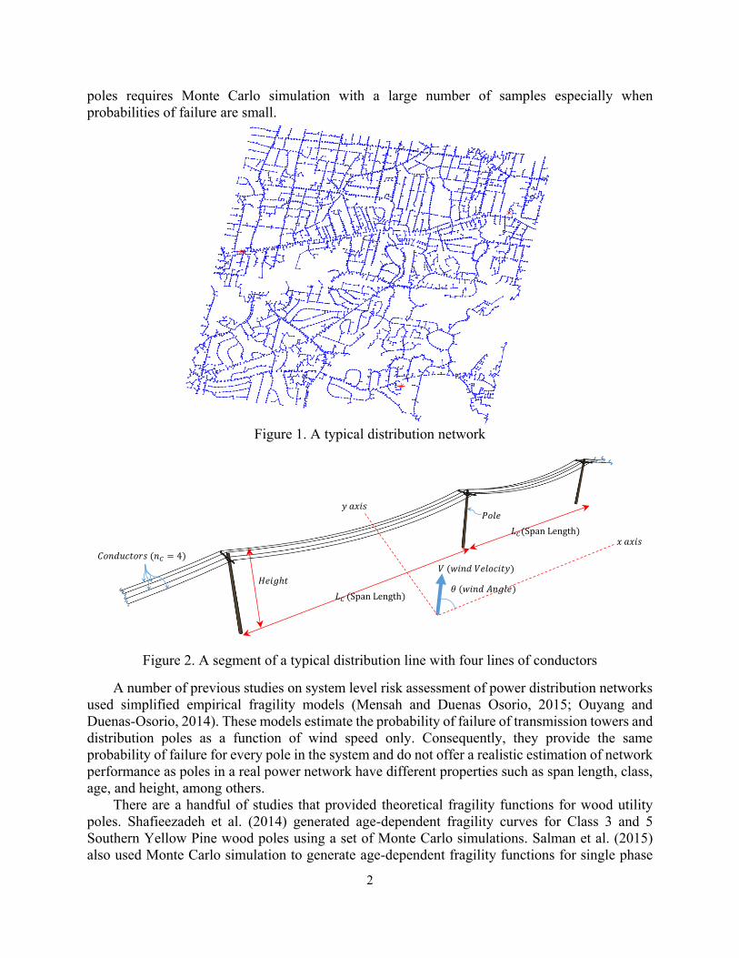
wood poles. A real distribution network, commonly, consists of thousands of poles. A typical

distribution network in southeast of US with about 7000 poles is shown in Fig. 1. Considering that

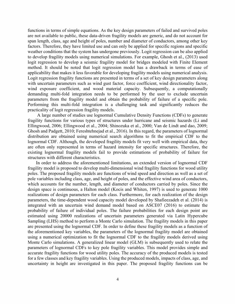
the properties of individual poles such as class and age of poles, number and diameter of

conductors, and span length (shown in Fig. 2) can change from one pole to another in a given

network, reliability analyses should be performed for each individual pole. This procedure

becomes significantly time consuming and computationally expensive as reliability analysis of

* Department of Civil, Environmental and Geodetic Engineering, Ohio State University, Columbus, US † Department of Civil, Environmental and Geodetic Engineering, Ohio State University, Columbus, US;

Corresponding author: Shafieezadeh.1@osu.edu;

2

poles requires Monte Carlo simulation with a large number of samples especially when

probabilities of failure are small.

Figure 1. A typical distribution network

Figure 2. A segment of a typical distribution line with four lines of conductors

A number of previous studies on system level risk assessment of power distribution networks

used simplified empirical fragility models (Mensah and Duenas Osorio, 2015; Ouyang and

Duenas-Osorio, 2014). These models estimate the probability of failure of transmission towers and

distribution poles as a function of wind speed only. Consequently, they provide the same

probability of failure for every pole in the system and do not offer a realistic estimation of network

performance as poles in a real power network have different properties such as span length, class,

age, and height, among others.

There are a handful of studies that provided theoretical fragility functions for wood utility

poles. Shafieezadeh et al. (2014) generated age-dependent fragility curves for Class 3 and 5

Southern Yellow Pine wood poles using a set of Monte Carlo simulations. Salman et al. (2015)

also used Monte Carlo simulation to generate age-dependent fragility functions for single phase

𝜃 (𝑤𝑖𝑛𝑑 𝐴𝑛𝑔𝑙𝑒)

𝑉 (𝑤𝑖𝑛𝑑 𝑉𝑒𝑙𝑜𝑐𝑖𝑡𝑦)

𝑥 𝑎𝑥𝑖𝑠

𝑦 𝑎𝑥𝑖𝑠

𝐻𝑒𝑖𝑔ℎ𝑡

𝑃𝑜𝑙𝑒

𝐿𝐶 (Span Length)

𝐿𝐶(Span Length)

𝐶𝑜𝑛𝑑𝑢𝑐𝑡𝑜𝑟𝑠 (𝑛𝐶 = 4)

3

and three phase line poles. However, these studies provide generic fragility models and therefore,

likelihoods of failure cannot be explicitly expressed in terms of key design parameters such as the

number and diameter of conductors, span length, and wind direction. It should be noted that these

fragility models were generated with specific assumptions about the configuration of poles and

lines. For example, in the fragility models provided by Shafieezadeh et al. (2014), it was assumed

that poles carry three conductors with a diameter of 11 mm. Moreover, the height of the poles and

the span of conductors in that study were considered to be random variables and follow lognormal

distributions. Similarly, in the fragility models by Salman et al. (2015), three lines of conductors

were considered where two of the conductors had a diameter of 18.3 mm and one of them had a

diameter of 11.8 mm. Span length was assumed to be 46 m and the poles were assumed to be 13.7

m high. These fragility models are only applicable to wood poles with similar configurations and

properties. In distribution networks, however, the number and size of conductors may vary.

Furthermore, wind direction in these studies was assumed to be perpendicular to conductors. This

represents the worst case scenario as the projected surface area of conductors is smaller for other

wind directions. Therefore, this assumption may lead to considerable overestimation of

probabilities of failure especially if the wind direction is nearly parallel to conductors. As an

example to highlight the limitation of the existing fragility models, consider two poles with similar

configurations but different span lengths. Assume that the first pole carries conductors with a span

length of 50 m and the second one carries conductors with a span length of 100 m. The existing

fragility functions are not able to distinguish between the probabilities of failure of these two poles

as they do not consider span length as an input parameter to the fragility model. Therefore, they

would provide identical probabilities of failure for both poles. The same trend applies to poles with

same classes but different heights, numbers and diameter of conductors. The aforementioned

variables considerably impact the wind reliability of poles, and they are rather easy to measure and

are available in most asset management databases, or can be accounted for via probabilistic

models. Consequently, fragility models for wood utility poles should consider these factors as

input variables in order to offer reliable estimates of the likelihood of failure of poles. In addition,

for risk reduction purposes, a key strengthening option is to replace vulnerable poles by new ones.

Fragility functions can assist with such decisions as they can provide estimates of the likelihood

of failure of poles. However, the existing generic fragility functions have limited applications in

this regard as they do not offer likelihoods of failure of poles as a function of key design variables,

which are often available for poles considered to be replaced.

Meta-modeling techniques have been successfully employed to generate fragility models in

terms of key characteristics of various types of structures under wind or seismic hazards (Ebad-

Sichani et al., 2018; Bhat et al., 2018). Recently, Bhat et al. (2018) used a meta-model based on

Kriging to estimate the probability of failure of a real distribution network composed of 7051 poles

with different ages, classes, and span lengths, among others. It should be mentioned that the

objective of this study is to provide a simple yet accurate multi-dimensional fragility model for

wood poles that is beneficial to users dealing with risk assessment of power distribution networks.

Meta-models, however, face a challenge in this regard as their form and parameters cannot be

simply presented in publications and therefore may not be accessible by the broader research

community.

Logit regression models have also been used to generate fragility functions for hurricane

hazards. For example, Reed et al., (2016) used a logit regression model to develop empirical multi-

hazard fragility models based on power outage data obtained from hurricanes Sandy and Isaac.

Unlike meta-modeling techniques such as Kriging, logit regression models can present fragility

4

functions in terms of simple equations. As the key design parameters of failed and survived poles

are not available to public, these data-driven fragility models are generic, and do not account for

span length, class, age and height of poles, number and diameter of conductors, among other key

factors. Therefore, they have limited use and can only be applied for specific regions and specific

weather conditions that the system has undergone previously. Logit regression can be also applied

to develop fragility models using numerical simulations. For example, Ghosh et al., (2013) used

logit regression to develop a seismic fragility model for bridges modeled with Finite Element

method. It should be noted that logit regression model has a drawback in terms of ease of

applicability that makes it less favorable for developing fragility models using numerical analysis.

Logit regression fragility functions are presented in terms of a set of key design parameters along

with uncertain parameters such as wind gust factor, force coefficient, wind directionality factor,

wind exposure coefficient, and wood material capacity. Subsequently, a computationally

demanding multi-fold integration needs to be performed by the user to exclude uncertain

parameters from the fragility model and obtain the probability of failure of a specific pole.

Performing this multi-fold integration is a challenging task and significantly reduces the

practicality of logit regression fragility models.

A large number of studies use lognormal Cumulative Density Functions (CDFs) to generate

fragility functions for various types of structures under hurricane and seismic hazards (Li and

Ellingwood, 2006; Ellingwood et al., 2004; Shinozuka et al., 2000; Van de Lindt and dao, 2009;

Ghosh and Padgett, 2010; Fereshtehnejad et al., 2016). In this regard, the parameters of lognormal

distribution are obtained using numerical search algorithms to fit the empirical CDF to the

lognormal CDF. Although, the developed fragility models fit very well with empirical data, they

are often only represented in terms of hazard intensity for specific structures. Therefore, the

existing lognormal fragility models fail to provide estimations of probability of failure for

structures with different characteristics.

In order to address the aforementioned limitations, an extended version of lognormal CDF

fragility model is proposed to develop multi-dimensional wind fragility functions for wood utility

poles. The proposed fragility models are functions of wind speed and direction as well as a set of

pole variables including class, age, and height of poles, and the effective wind area of conductors,

which accounts for the number, length, and diameter of conductors carried by poles. Since the

design space is continuous, a Halton model (Kocis and Whiten, 1997) is used to generate 1000

realizations of design parameters for each class. Furthermore, for each realization of the design

parameters, the time-dependent wood capacity model developed by Shafieezadeh et al. (2014) is

integrated with an uncertain wind demand model based on ASCE07 (2016) to estimate the

probability of failure of individual poles. The failure probabilities for each design point are

estimated using 20000 realizations of uncertain parameters generated via Latin Hypercube

Sampling (LHS) method to perform a Monte Carlo simulation. The fragility models in this paper

are presented using the lognormal CDF. In order to define these fragility models as a function of

the aforementioned key variables, the parameters of the lognormal fragility model are obtained

using a numerical optimization to fit the lognormal CDF to the fragility models derived using

Monte Carlo simulations. A generalized linear model (GLM) is subsequently used to relate the

parameters of lognormal CDFs to key pole fragility variables. This model provides simple and

accurate fragility functions for wood utility poles. The accuracy of the produced models is tested

for a few classes and key fragility variables. Using the produced models, impacts of class, age, and

uncertainty in height are investigated in this paper. The proposed fragility functions can be

5

integrated with wind hazard models to perform a system level reliability analysis and analyze the

reliability and resilience of power distribution networks.

2. RELIABILITY ANALYSIS OF WOOD UTILITY POLES

Performance of wood utility poles depends on a set of uncertain parameters, which define the

demand and capacity of the system. As it was mentioned previously, for risk assessment purposes,

there is a high demand to probabilistically evaluate the performance of wood poles. Commonly,

the uncertain performance of systems is defined by a binary random variable, which describes the

event of failure or success in meeting a specific performance level. The metric that quantifies

failure or survival is called the limit state function (𝐺(𝑋)). For wood poles, the limit state function

is often defined as:

𝐺(𝑋) = 𝑀𝑅(𝑋) − 𝑀𝑆(𝑋) (1)

where 𝑀𝑅 stands for the moment capacity of wood pole, 𝑀𝑆 is the moment demand on the wood

pole, and X is a set of random variables involved in the limit state function. When 𝐺(𝑋) < 0, the

wood pole is considered as failed. The probability of failure for wood poles can be derived as:

𝑃𝑓 = 𝑃[𝐺(𝑋) < 0] = ∫ 𝑃[𝐺(𝑋) < 0|𝑣 = 𝑦] 𝑓𝑣(𝑦)𝑑𝑦

𝑦

(2)

where 𝑣 is the random variable defining wind speed, 𝑓𝑣(𝑦) is the probability density function of

the wind speed, and 𝑃[𝐺(𝑋) < 0|𝑣 = 𝑦] is called the fragility function, which defines the

conditional probability of failure given that 𝑣 = 𝑦.

In a power distribution network, since the properties of individual poles are different from one

another, performance assessment of the distribution network requires an expensive and time

consuming reliability analysis for each individual component of the system. Individual reliability

analyses for the significantly large number of utility poles can be avoided using multi-dimensional

fragility functions, which describe the likelihood of failure as a function of key design parameters

while considering uncertainties in other variables. This section elaborates the procedure to obtain

the probability of failure of individual wood poles. The obtained probabilities of failure are used

in the upcoming sections to develop multi-dimensional fragility functions.

2.1. Demand Model for Wood Poles

Failure can occur at any location of a wood pole. However, experience from past hazard events

confirm that 90% of wood pole failures occur at the ground line (Li et al., 2005; Sandoz et al.

1997). Estimating the exact failure location requires comparing the moment demand and moment

capacity at various elevations of the pole, which makes the estimation of failure probability a

challenging task. In addition, the rate of decay in the wood material increases with exposure to

moisture and oxygen and therefore, the ground line has a significantly higher rate of decay as it

can absorb moisture from the soil. Subsequently, failure at the ground line is the dominant mode

of failure. Therefore, in this study, the failure is assumed as the event that the wind-induced

moment at the ground line exceeds the moment capacity of the pole at the ground line. This mode

of failure has been extensively used in the previous studies on the reliability analysis of wood poles

(Salman et al., 2015; Ryan et al., 2014; Bhat et al., 2018; Onyewuchi et al., 2015; Shafieezadeh et

al. 2014; Darestani et al., 2016a; Darestani et al. 2016b; Darestani et al. 2017; Darestani and

Shafieezadeh, 2017). In addition, the buried length of the pole is also important since it affects the

overturning moment capacity of the pole caused by foundation failures. However, since the

foundation failure is not investigated in this study, the embedded length is excluded from the

fragility models. Subsequently, any loading contributing to the induced moment at the ground line

6

should be considered in the demand model. In a distribution line that adjacent poles are coupled to

one another through conductors, the actual demand is a function of properties of the pole of interest

and the attached conductors as well as the properties of adjacent spans. Through a few studies,

authors showed that if the properties of adjacent poles are noticeably different from one another,

the demand and capacity of adjacent poles contribute to the demand and capacity of the pole of

interest due to structural couplings (Darestani et al., 2016a; Darestani et al. 2016b; Darestani et al.

2017). On the other hand, in order to consider the effect of adjacent spans, the specific properties

of adjacent poles should be available. Since the goal of this study is to provide simple yet accurate

fragility functions that can be easily used to estimate the probability of failure of various wood

poles, effects of adjacent spans are not considered here. Subsequently, the demand is calculated as

the sum of the moments induced by wind effects on the pole of interest and attached conductors.

It should be noted that the performance of wood poles is also affected by inundation due to storm

surge and rainfall. Flooding can apply a large lateral force and cause failure of the pole itself.

However, in this study this effect is not considered, as this study focuses on wind-driven damage

to poles. Inundation-induced failures will be addressed in future research. Furthermore, to estimate

the wind performance of wood poles, a static equivalent wind load model based on ASCE07 (2016)

is considered in this study, which is widely accepted for wind performance analysis of poles and

conductors (Salman et al., 2015; Ryan et al., 2014, Bhat et al., 2018; Onyewuchi et al., 2015;

Shafieezadeh et al. 2014). Dynamic effects are approximately captured in the static equivalent

model via a 3-second gust wind velocity along with gust factor and force coefficients. Moreover,

given the significantly large number of simulations (20,000) that are required for fragility analysis

for each realization of the covariate set, performing nonlinear dynamic analyses to generate

fragility models will not be practically feasible. A possible solution to overcome this issue is to

perform adaptive Kriging-based reliability analysis (Wang and Shafieezadeh, 2018) to estimate

the probability of failure of wood poles efficiently. However, using advanced adaptive reliability

methods along with nonlinear time history analysis is beyond the scope of this paper.

According to ASCE07 (2016), the wind force per unit length for a non-building structure

can be determined using:

𝑓𝑤(𝑧) = 𝑞𝑧(𝑧)𝐺𝐶𝑓(𝑧)𝐷(𝑧) (3)

where 𝑞𝑧 is the velocity pressure at height 𝑧 on the pole or conductor, 𝐺 is the gust-effect factor,

𝐶𝑓 is the force coefficient, and 𝐷 is the diameter of pole or conductor perpendicular to the wind

direction. The velocity pressure is obtained from:

𝑞𝑧 = 0.613𝐾𝑧(𝑧)𝐾𝑑𝐾𝑧𝑡𝐾𝑒𝑉𝑝2 (4)

where 𝐾𝑧 is the velocity pressure exposure coefficient, 𝐾𝑑 is the wind directionality factor, 𝐾𝑧𝑡 is

the topographic factor, 𝐾𝑒 is the elevation factor and 𝑉𝑝 is the projected 3-second gust wind speed

at 10 m height above the ground. Since in this study it is assumed that the distribution line is

located in a flat area, according to ASCE07 (2016), 𝐾𝑧𝑡 is equal to one. According to this code,

𝐾𝑧 is a function of the height from the ground-line and exposure category, and can be obtained

from:

𝐾𝑧(𝑧) = 2.01 (max (4.6, 𝑧)

𝑧𝑔)

2/𝛼

(5)

It is assumed that the distribution line is located in an open terrain area; therefore, the exposure

category according to ASCE07 (2016) is C, and 𝛼 and 𝑧𝑔 are 9.5 and 274.32 m, respectively. The

7

wind directionality factor 𝐾𝑑 and elevation factor 𝐾𝑒 are both 1 and the gust-effect factor 𝐺 for

rigid structures is 0.85 (ASCE07, 2016). The force coefficient 𝐶𝑓 depends on the surface

roughness, the height-to-diameter ratio, and velocity pressure 𝑞𝑧. For wood poles, force coefficient

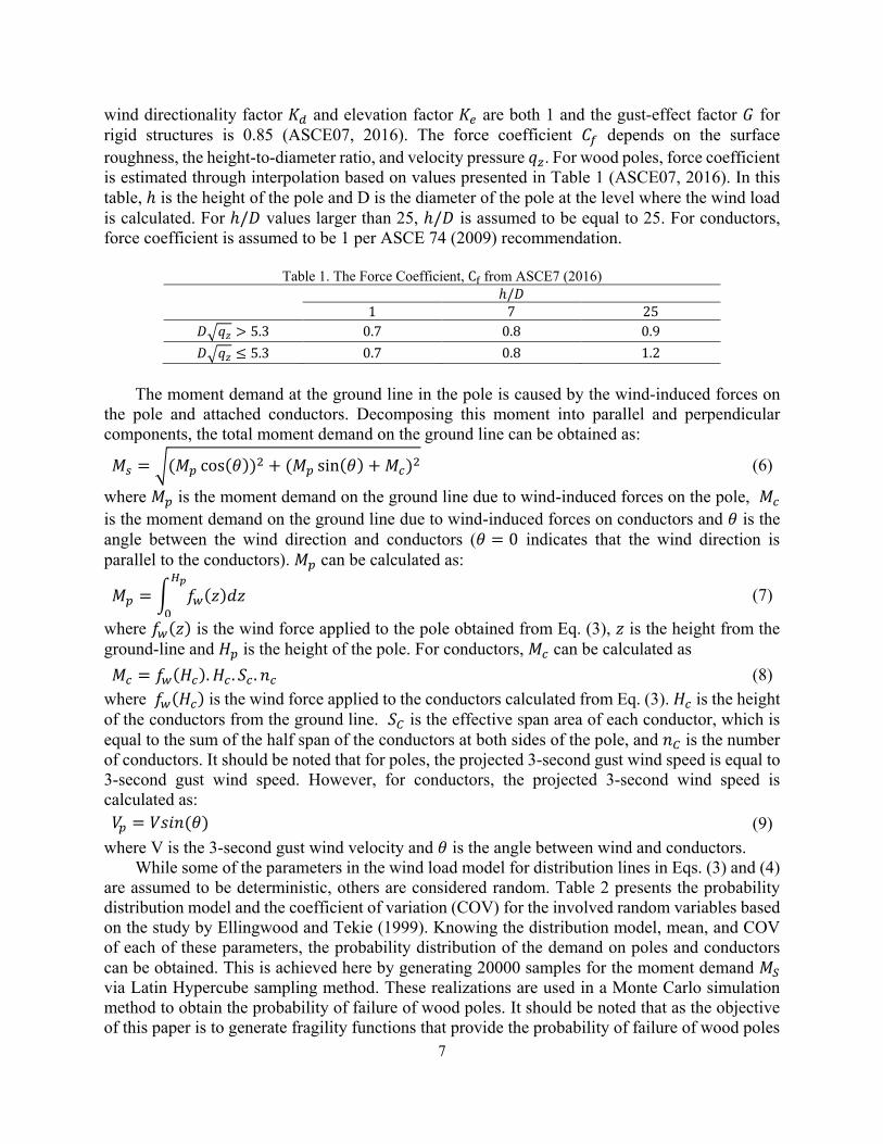
is estimated through interpolation based on values presented in Table 1 (ASCE07, 2016). In this

table, ℎ is the height of the pole and D is the diameter of the pole at the level where the wind load

is calculated. For ℎ/𝐷 values larger than 25, ℎ/𝐷 is assumed to be equal to 25. For conductors,

force coefficient is assumed to be 1 per ASCE 74 (2009) recommendation.

Table 1. The Force Coefficient, Cf from ASCE7 (2016)

ℎ/𝐷

1 7 25

𝐷√𝑞𝑧 > 5.3 0.7 0.8 0.9

𝐷√𝑞𝑧 ≤ 5.3 0.7 0.8 1.2

The moment demand at the ground line in the pole is caused by the wind-induced forces on

the pole and attached conductors. Decomposing this moment into parallel and perpendicular

components, the total moment demand on the ground line can be obtained as:

𝑀𝑠 = √(𝑀𝑝 cos(𝜃))2 + (𝑀𝑝 sin(𝜃) + 𝑀𝑐)2 (6)

where 𝑀𝑝 is the moment demand on the ground line due to wind-induced forces on the pole, 𝑀𝑐

is the moment demand on the ground line due to wind-induced forces on conductors and 𝜃 is the

angle between the wind direction and conductors (𝜃 = 0 indicates that the wind direction is

parallel to the conductors). 𝑀𝑝 can be calculated as:

𝑀𝑝 = ∫ 𝑓𝑤(𝑧)𝑑𝑧𝐻𝑝

0

(7)

where 𝑓𝑤(𝑧) is the wind force applied to the pole obtained from Eq. (3), 𝑧 is the height from the

ground-line and 𝐻𝑝 is the height of the pole. For conductors, 𝑀𝑐 can be calculated as

𝑀𝑐 = 𝑓𝑤(𝐻𝑐). 𝐻𝑐 . 𝑆𝑐 . 𝑛𝑐 (8)

where 𝑓𝑤(𝐻𝑐) is the wind force applied to the conductors calculated from Eq. (3). 𝐻𝑐 is the height

of the conductors from the ground line. 𝑆𝐶 is the effective span area of each conductor, which is

equal to the sum of the half span of the conductors at both sides of the pole, and 𝑛𝐶 is the number

of conductors. It should be noted that for poles, the projected 3-second gust wind speed is equal to

3-second gust wind speed. However, for conductors, the projected 3-second wind speed is

calculated as:

𝑉𝑝 = 𝑉𝑠𝑖𝑛(𝜃) (9)

where V is the 3-second gust wind velocity and 𝜃 is the angle between wind and conductors.

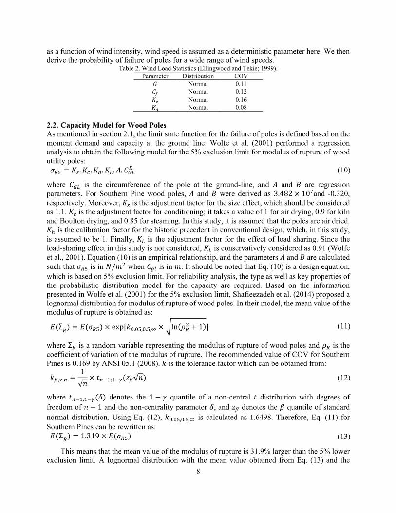
While some of the parameters in the wind load model for distribution lines in Eqs. (3) and (4)

are assumed to be deterministic, others are considered random. Table 2 presents the probability

distribution model and the coefficient of variation (COV) for the involved random variables based

on the study by Ellingwood and Tekie (1999). Knowing the distribution model, mean, and COV

of each of these parameters, the probability distribution of the demand on poles and conductors

can be obtained. This is achieved here by generating 20000 samples for the moment demand 𝑀𝑆

via Latin Hypercube sampling method. These realizations are used in a Monte Carlo simulation

method to obtain the probability of failure of wood poles. It should be noted that as the objective

of this paper is to generate fragility functions that provide the probability of failure of wood poles

8

as a function of wind intensity, wind speed is assumed as a deterministic parameter here. We then

derive the probability of failure of poles for a wide range of wind speeds. Table 2. Wind Load Statistics (Ellingwood and Tekie; 1999).

Parameter Distribution COV

𝐺 Normal 0.11

𝐶𝑓 Normal 0.12

𝐾𝑧 Normal 0.16

𝐾𝑑 Normal 0.08

2.2. Capacity Model for Wood Poles

As mentioned in section 2.1, the limit state function for the failure of poles is defined based on the

moment demand and capacity at the ground line. Wolfe et al. (2001) performed a regression

analysis to obtain the following model for the 5% exclusion limit for modulus of rupture of wood

utility poles:

𝜎𝑅5 = 𝐾𝑠. 𝐾𝑐 . 𝐾ℎ. 𝐾𝐿 . 𝐴. 𝐶𝐺𝐿𝐵 (10)

where 𝐶𝐺𝐿 is the circumference of the pole at the ground-line, and 𝐴 and 𝐵 are regression

parameters. For Southern Pine wood poles, 𝐴 and 𝐵 were derived as 3.482 × 107and -0.320,

respectively. Moreover, 𝐾𝑠 is the adjustment factor for the size effect, which should be considered

as 1.1. 𝐾𝑐 is the adjustment factor for conditioning; it takes a value of 1 for air drying, 0.9 for kiln

and Boulton drying, and 0.85 for steaming. In this study, it is assumed that the poles are air dried.

𝐾ℎ is the calibration factor for the historic precedent in conventional design, which, in this study,

is assumed to be 1. Finally, 𝐾𝐿 is the adjustment factor for the effect of load sharing. Since the

load-sharing effect in this study is not considered, 𝐾𝐿 is conservatively considered as 0.91 (Wolfe

et al., 2001). Equation (10) is an empirical relationship, and the parameters 𝐴 and 𝐵 are calculated

such that 𝜎𝑅5 is in 𝑁/𝑚2 when 𝐶𝑔𝑙 is in 𝑚. It should be noted that Eq. (10) is a design equation,

which is based on 5% exclusion limit. For reliability analysis, the type as well as key properties of

the probabilistic distribution model for the capacity are required. Based on the information

presented in Wolfe et al. (2001) for the 5% exclusion limit, Shafieezadeh et al. (2014) proposed a

lognormal distribution for modulus of rupture of wood poles. In their model, the mean value of the

modulus of rupture is obtained as:

𝐸(Σ𝑅

) = 𝐸(𝜎𝑅5) × exp [𝑘0.05,0.5,∞ × √ln(𝜌𝑅2 + 1)] (11)

where Σ𝑅 is a random variable representing the modulus of rupture of wood poles and 𝜌𝑅 is the

coefficient of variation of the modulus of rupture. The recommended value of COV for Southern

Pines is 0.169 by ANSI 05.1 (2008). 𝑘 is the tolerance factor which can be obtained from:

𝑘𝛽,𝛾,𝑛 =1

√𝑛× 𝑡𝑛−1;1−𝛾(𝑧𝛽√𝑛) (12)

where 𝑡𝑛−1;1−𝛾(𝛿) denotes the 1 − 𝛾 quantile of a non-central 𝑡 distribution with degrees of

freedom of 𝑛 − 1 and the non-centrality parameter 𝛿, and 𝑧𝛽 denotes the 𝛽 quantile of standard

normal distribution. Using Eq. (12), 𝑘0.05,0.5,∞ is calculated as 1.6498. Therefore, Eq. (11) for

Southern Pines can be rewritten as:

𝐸(Σ𝑅

) = 1.319 × 𝐸(𝜎𝑅5) (13)

This means that the mean value of the modulus of rupture is 31.9% larger than the 5% lower

exclusion limit. A lognormal distribution with the mean value obtained from Eq. (13) and the

9

coefficient of variation of 0.169 is used to generate realizations of modulus of rupture of wood

poles. The modulus of rupture is then converted to the moment capacity at the ground line using

the following equation:

𝑀𝑅 =Σ𝑅 . 𝐶𝑔𝑙

3

32. 𝜋2 (14)

where Σ𝑅 is the modulus of rupture of the pole at the ground line and 𝐶𝑔𝑙 is the circumference of

the pole at the ground line. The realizations obtained for 𝑀𝑅 are compared with the realizations of

moment demand calculated from Eq. (6) in a Monte Carlo simulation method to obtain the

probability of failure of poles. It should be noted that wood poles are made of various tree species

such as Southern Yellow Pine, Douglas Fair, and Western Red Cedar, among others. The fragility

models in this study are developed for Southern Yellow Pine wood poles as they are the most

common wood pole species (Salman et al. 2015) in addition to the fact that time-dependent

capacity models have not been developed for other wood pole species. The fragility models for

other species of wood poles can be generated using a similar procedure proposed by Shafieezadeh

et al., (2014) when associated time-dependent capacity models are available.

2.3. Effects of In-Service Decay on the Capacity of Poles

The ground line section of utility poles is exposed the most to the moisture from the ground. This

leads to a high rate of decay of wood poles at the ground level (Shafieezadeh et al., 2014). Because

of the high moment demand and high rate of decay, the failure of poles is more likely to occur at

the ground line section. Li et al. (2005) used a series of nondestructive tests on 13940 wood poles

to perform a regression analysis to develop linear age dependent models that can predict the

percentage of decayed poles and the strength loss for wood poles. Shafieezadeh et al. (2014)

observed that the initial linear model underestimates the percentage of decayed poles for pole with

ages more than 40 years old. Therefore, they suggested a power model based on the original non-

destructive tests reported by Li et al., (2005). Subsequently, Shafieezadeh et al. (2014), used the

linear model for strength loss and the power model for the percentage of decayed poles to develop

an age-dependent model for mean and variance of the capacity of Southern Yellow Pine wood

poles. According to this model, the mean and variance of the capacity of wood poles are functions

of the capacity of new wood poles and the age of the pole as follows:

𝐸[𝑀𝑅|𝑇 = 𝑡] = 𝐸[𝑀𝑅0][1 − min(max(𝑎1𝑡 − 𝑎2, 0) , 1) × min(max(𝑏′

1𝑡𝑏′2 , 0) , 1)] (15)

𝑉𝑎𝑟[𝑀𝑅|𝑇 = 𝑡] = (𝑉𝑎𝑟[𝑀𝑅0] + 𝐸[𝑀𝑅0

]2

) (1 − min(max(𝑏′1𝑡𝑏′

2 , 0) , 1)) + {(𝑉𝑎𝑟[𝑀𝑅0] + 𝐸[𝑀𝑅0

]2

)

[𝑉𝑎𝑟[𝐿|𝑇] + (1 − min(max(𝑎1𝑡 − 𝑎2, 0) , 1))2]} × (min(max(𝑏′1𝑡𝑏′

2 , 0) , 1))

−𝐸[𝑀𝑅0]

2× [1 − min(max(𝑎1𝑡 − 𝑎2, 0) , 1) × min(max(𝑏′

1𝑡𝑏′2 , 0) , 1)]2

(16)

where 𝑀𝑅 is the moment capacity of wood poles, 𝑀𝑅0 is the moment capacity of new poles, 𝑡 is

the age of the wood pole in terms of years, and 𝑉𝑎𝑟[𝐿|𝑇] is the time-dependent variance of the

loss of the capacity of wood poles. Based on the data reported by Li et al. (2005), this parameter

is set as 0.11. Parameters 𝑎1 and 𝑎2 represent the percentage of strength loss for wood poles.

According to a regression analysis performed by Li et al. (2005), these parameters are found as

0.014418 and 0.10683, respectively. Parameters 𝑏′1 and 𝑏′

2 account for the percentage of decayed

poles. Based on a regression analysis performed by Shafieezadeh et al. (2014), there parameters

are found as 0.00013 and 1.846, respectively. Furthermore, as wood poles especially Southern

Yellow Pines are vulnerable against decay, they are usually treated by preservatives. There are two

different classes of wood preservatives: oil-based and water-based (Ibach, 1999). The rate of decay

in wood poles is affected by the type and amount of preservatives used in the treatment process.

10

As it was noted previously, the time-dependent model for Southern Yellow Pine was developed

using a series of nondestructive tests reported by Li et al. (2005) on 13940 wood poles. The wood

poles used in that study appear to had been treated with various preservatives and the treatment

type is not available for the tested poles. Therefore, the impact of various preservatives on the rate

of decay of poles cannot be individually investigated. It can be concluded that the time-dependent

wood pole capacity model developed by Shafieezadeh et al. (2014) is a practical solution where

the treatment type of wood poles is uncertain.

3. MULTI-DIMENSIONAL FRAGILITY FUNCTIONS

As noted previously, fragility models are essential components for risk analysis of infrastructure

systems including the power grid. The performance of each individual pole in a distribution line

is a function of a set of design (input) parameters such as class, age, and height of poles, number,

diameter and length of conductors and a set of uncertain parameters such as wind directionality

factor, gust factor, wind exposure coefficient, force coefficient, and modulus of rupture of wood

poles. For each individual pole, there is a unique set of design parameters that differentiates that

pole from the other poles in the network. However, the existing fragility curves only account for

the class and age of the poles, and other design parameters are usually assumed as uncertain or

fixed in the fragility analysis. Therefore, they may not provide accurate estimates of the probability

of failure of individual poles. In order to address these limitations, the current study, for the first

time, develops a set of multi-dimensional fragility functions that account for wind speed and its

direction, class, age, and height of poles, and number, diameter, and length of conductors.

A part of a typical distribution line is shown in Fig.2. Since the moment demand at the ground

line of poles is a direct function of the product of span length (length of conductors), number of

conductors, and diameter of conductors, a new design parameter called Conductor Area is defined

to reduce the number of design parameters.

𝐴𝐶 = 𝑛𝐶𝑑𝐶𝐿𝐶 (17)

where 𝑛𝐶, 𝑑𝐶, and 𝐿𝐶 are the diameter and number of conductors, and the span length, respectively.

Considering these variables individually does not offer any advantage in developing fragility

models as only the multiplication of these parameters is important for wind-induced moments and

subsequently the probability of failure of wood poles. Subsequently, the fragility models are

defined as a function of wind speed, wind direction, class, age, and height of poles and conductor

area. It should be noted that in some cases, information about some of the design variables may

not be available. One such factor is the height of the poles which can serve as design variable if

information about the height is available, otherwise as an uncertain variable. Given the importance

of height for fragility of the poles, in this study, height is one time treated as design variable in the

fragility functions and another time as a random variable by considering the uncertainty in the

height of each class of poles. In addition, for the reliability analysis, it is necessary to have

realizations of pole diameter at the top and at ground level. ANSI O5.1 (2008) provides the

minimum circumference at top and at 1.83 m from the bottom as a function of class and height of

poles. From the pole minimum circumference provided from ANSI O5.1, it is obvious that for a

given height, the minimum circumference decreases as the class number increases. According to

Shafieezadeh et al., (2014) the circumference for class 𝑖 is assumed to follow a uniform distribution

with a minimum and maximum value equal to the minimum circumference of class 𝑖 and class 𝑖 −1, respectively. In order to generate realizations of height and diameter for each class of poles, a

database of 769999 Southern Yellow Pine poles in southeast of US is considered in this study.

11

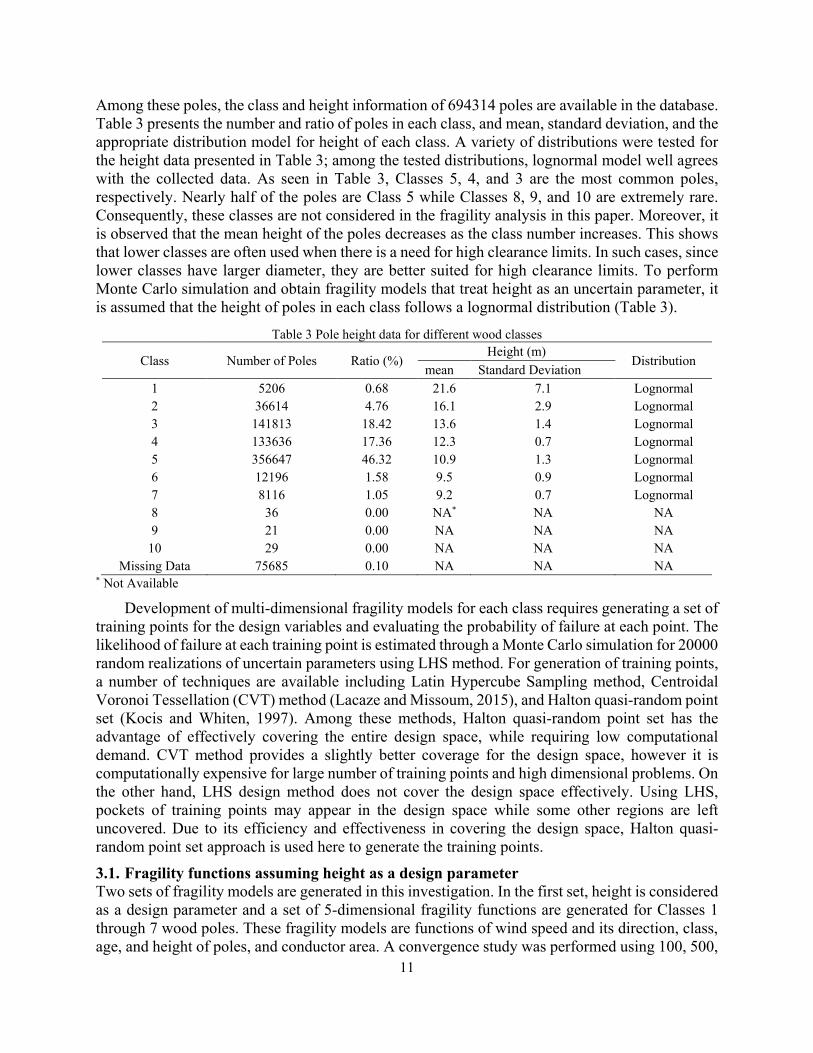
Among these poles, the class and height information of 694314 poles are available in the database.

Table 3 presents the number and ratio of poles in each class, and mean, standard deviation, and the

appropriate distribution model for height of each class. A variety of distributions were tested for

the height data presented in Table 3; among the tested distributions, lognormal model well agrees

with the collected data. As seen in Table 3, Classes 5, 4, and 3 are the most common poles,

respectively. Nearly half of the poles are Class 5 while Classes 8, 9, and 10 are extremely rare.

Consequently, these classes are not considered in the fragility analysis in this paper. Moreover, it

is observed that the mean height of the poles decreases as the class number increases. This shows

that lower classes are often used when there is a need for high clearance limits. In such cases, since

lower classes have larger diameter, they are better suited for high clearance limits. To perform

Monte Carlo simulation and obtain fragility models that treat height as an uncertain parameter, it

is assumed that the height of poles in each class follows a lognormal distribution (Table 3).

Table 3 Pole height data for different wood classes

Class Number of Poles Ratio (%) Height (m)

Distribution mean Standard Deviation

1 5206 0.68 21.6 7.1 Lognormal

2 36614 4.76 16.1 2.9 Lognormal

3 141813 18.42 13.6 1.4 Lognormal

4 133636 17.36 12.3 0.7 Lognormal

5 356647 46.32 10.9 1.3 Lognormal

6 12196 1.58 9.5 0.9 Lognormal

7 8116 1.05 9.2 0.7 Lognormal

8 36 0.00 NA* NA NA

9 21 0.00 NA NA NA

10 29 0.00 NA NA NA

Missing Data 75685 0.10 NA NA NA * Not Available

Development of multi-dimensional fragility models for each class requires generating a set of

training points for the design variables and evaluating the probability of failure at each point. The

likelihood of failure at each training point is estimated through a Monte Carlo simulation for 20000

random realizations of uncertain parameters using LHS method. For generation of training points,

a number of techniques are available including Latin Hypercube Sampling method, Centroidal

Voronoi Tessellation (CVT) method (Lacaze and Missoum, 2015), and Halton quasi-random point

set (Kocis and Whiten, 1997). Among these methods, Halton quasi-random point set has the

advantage of effectively covering the entire design space, while requiring low computational

demand. CVT method provides a slightly better coverage for the design space, however it is

computationally expensive for large number of training points and high dimensional problems. On

the other hand, LHS design method does not cover the design space effectively. Using LHS,

pockets of training points may appear in the design space while some other regions are left

uncovered. Due to its efficiency and effectiveness in covering the design space, Halton quasi-

random point set approach is used here to generate the training points.

3.1. Fragility functions assuming height as a design parameter

Two sets of fragility models are generated in this investigation. In the first set, height is considered

as a design parameter and a set of 5-dimensional fragility functions are generated for Classes 1

through 7 wood poles. These fragility models are functions of wind speed and its direction, class,

age, and height of poles, and conductor area. A convergence study was performed using 100, 500,

12

and 1000 realizations of uncertain parameters. The results showed that the difference in the

fragility models for 500 and 1000 realizations cases were insignificant. Therefore, a set of 1000

realizations of wind direction, age and height of poles, and conductor areas were generated using

Halton quasi-random point sets. Ranges of parameters used for generating the training points are

provided in Table 4. Subsequently, for each training point, the probability of failure of the pole is

estimated for wind speeds of 5 to 250 mph with a step size of 5 mph. A lognormal CDF is fitted

to the fragility curve obtained for each set of training points using a numerical search based on the

least square method. The lognormal CDF has the following form:

𝑃[𝐺(𝑋) < 0|𝑉, 𝑡, 𝜃, 𝐴𝐶 , 𝐻] = Φ (ln(𝑉) − 𝜇(𝑡, 𝜃, 𝐴𝐶 , 𝐻)

𝜎(𝑡, 𝜃, 𝐴𝐶 , 𝐻)) (18)

where 𝑉 is the wind speed, and 𝜇 and 𝜎 are the parameters of lognormal distribution, respectively.

For each set of training points, the values of 𝜇 and 𝜎 are recorded. A response surface is then fitted

to these parameters for the entire set of training points. The response surface has the following

form:

𝜇 𝑜𝑟 𝜎 = 𝑎0 + 𝑎1𝜃 + 𝑎2𝐴𝐶 + 𝑎3𝑡 + 𝑎4𝐻 + 𝑎5𝜃2 + 𝑎6𝐴𝐶. 𝜃+𝑎7𝐴𝐶2 + 𝑎8𝑡. 𝜃 + 𝑎9𝑡. 𝐴𝐶 + 𝑎10𝑡2

+ 𝑎11𝜃. 𝐻 + 𝑎12𝐴𝐶. 𝐻 + 𝑎13𝑡. 𝐻 + 𝑎14𝐻2 (19)

where 𝑎𝑖 (𝑖 = 0, … ,14) are the contribution of each term in the response surface, 𝑡 is the modified

age of the pole (in years) that is explained in the next paragraph, 𝜃 is the wind direction (in degree),

𝐴𝐶 is the conductor area (m2), and 𝐻 is the height of the pole (in m).

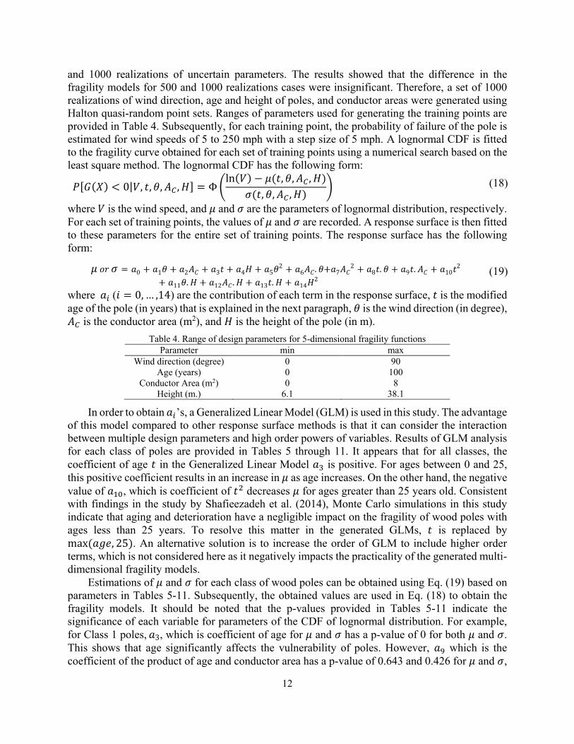
Table 4. Range of design parameters for 5-dimensional fragility functions Parameter min max

Wind direction (degree) 0 90

Age (years) 0 100

Conductor Area (m2)

Height (m.)

0

6.1

8

38.1

In order to obtain 𝑎𝑖’s, a Generalized Linear Model (GLM) is used in this study. The advantage

of this model compared to other response surface methods is that it can consider the interaction

between multiple design parameters and high order powers of variables. Results of GLM analysis

for each class of poles are provided in Tables 5 through 11. It appears that for all classes, the

coefficient of age 𝑡 in the Generalized Linear Model 𝑎3 is positive. For ages between 0 and 25,

this positive coefficient results in an increase in 𝜇 as age increases. On the other hand, the negative

value of 𝑎10, which is coefficient of 𝑡2 decreases 𝜇 for ages greater than 25 years old. Consistent

with findings in the study by Shafieezadeh et al. (2014), Monte Carlo simulations in this study

indicate that aging and deterioration have a negligible impact on the fragility of wood poles with

ages less than 25 years. To resolve this matter in the generated GLMs, 𝑡 is replaced by

max (𝑎𝑔𝑒, 25). An alternative solution is to increase the order of GLM to include higher order

terms, which is not considered here as it negatively impacts the practicality of the generated multi-

dimensional fragility models.

Estimations of 𝜇 and 𝜎 for each class of wood poles can be obtained using Eq. (19) based on

parameters in Tables 5-11. Subsequently, the obtained values are used in Eq. (18) to obtain the

fragility models. It should be noted that the p-values provided in Tables 5-11 indicate the

significance of each variable for parameters of the CDF of lognormal distribution. For example,

for Class 1 poles, 𝑎3, which is coefficient of age for 𝜇 and 𝜎 has a p-value of 0 for both 𝜇 and 𝜎.

This shows that age significantly affects the vulnerability of poles. However, 𝑎9 which is the

coefficient of the product of age and conductor area has a p-value of 0.643 and 0.426 for 𝜇 and 𝜎,

13

respectively. Since these values are larger than 0.05, the product of age and conductor area is an

insignificant parameter that does not noticeably contribute to the likelihood of failure of Class 1

wood poles. In GLM analysis provided in Tables 5-11, parameters with p-values of larger than

0.05 can be dropped from Eq. (19). Further investigation on the p-values provided in Tables 5-11

for all pole classes shows that first and second power of each design variable significantly

contributes to the likelihood of failure of poles. On the other hand, it turns out that the product of

age and conductor area and the product of age and wind direction are not significant. Therefore,

these factor can be neglected in Eq. (19). Moreover, for Classes 1-4, the p-values for 𝑎13, which

defines the contribution of the product of age and height are larger than 0.05 indicating that this

factor is not significant as well.

In addition, R2 values for the GLM analysis for each class are provided in Tables 5-11. For all

classes, R2 is greater than 0.979, which shows that the GLM method offers accurate estimates of

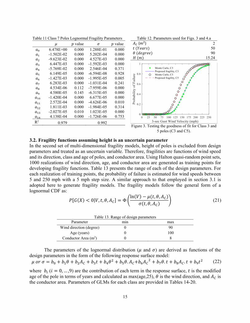
the parameters of the fragility functions. To further investigate the goodness of fit of the produced

GLM response surfaces, a comparison between the results obtained from Eqs. (18-19) for Classes

3 and 5 with raw fragility points obtained from Monte Carlo simulations is presented in Fig. 3.

The design parameters used in this figure are provided in Table 12. It is observed that the fitted

lognormal fragility model can accurately estimate the probability of failure of the pole. For

example, for a wind speed equal to 150 mph, the fragility function obtained from Monte Carlo

simulation results in a probability of failure equal to 0.34 and 0.64 for Classes 3 and 5, respectively.

When Eqs. (18-19) are used, these values become 0.34 and 0.62 for Classes 3 and 5, respectively.

The small errors confirm the accuracy of the proposed fragility model. For other points in the

design space, the same trend is observed.

It should be noted that the multi-dimensional fragility functions provided in this study can be

integrated with probabilistic models for wind direction, age, and other design parameters to

generate lower dimensional fragility functions. This procedure is applied when data for these

variables are not available for individual poles, but probabilistic models for a group of poles are

available. In such cases, the following integration can be implemented to provide 1-dimensional

fragility functions:

𝑃[𝐺(𝑋) < 0|𝑤] = ∬ ∬ 𝑃[𝐺(𝑋) < 0|𝑤, 𝑡 = 𝑦1, 𝜃 = 𝑦2, 𝐴𝐶 = 𝑦3, 𝐻 = 𝑦4]. 𝑓𝑡𝑟(𝑦1). 𝑓𝜃(𝑦2) . 𝑓𝐴𝐶

(𝑦3)

. 𝑓𝐻(𝑦4) 𝑑𝑦1𝑑𝑦2𝑑𝑦3𝑑𝑦4

(20)

where 𝑓𝑡(𝑦1), 𝑓𝜃(𝑦2), 𝑓𝐴𝐶(𝑦3), and 𝑓𝐻(𝑦4) are the probability distribution functions of age, wind

direction, conductor area, and height, respectively. A similar approach can be used to obtain 2-

dimensional, and 3-dimensional fragility functions.

14

Table 6. Class 2 Poles Lognormal Fragility Parameters 𝜇 𝑝 value 𝜎 𝑝 value

𝑎0 6.746E+00 0.000 1.558E-01 0.000

𝑎1 -1.064E-02 0.000 1.138E-04 0.049

𝑎2 -6.855E-02 0.000 9.836E-04 0.120

𝑎3 6.348E-03 0.000 -2.223E-03 0.000

𝑎4 -6.693E-02 0.000 6.356E-05 0.731

𝑎5 3.592E-05 0.000 -4.662E-07 0.323

𝑎6 -1.272E-03 0.000 4.661E-06 0.315

𝑎7 4.316E-03 0.000 -5.746E-05 0.314

𝑎8 -1.075E-06 0.659 5.576E-07 0.133

𝑎9 -1.330E-05 0.620 3.573E-06 0.382

𝑎10 -1.347E-04 0.000 6.485E-05 0.000

𝑎11 2.306E-04 0.000 -2.727E-06 0.019

𝑎12 1.670E-03 0.000 -2.260E-05 0.077

𝑎13 -7.642E-06 0.255 6.245E-06 0.000

𝑎14 5.307E-04 0.000 1.338E-06 0.707

R2 0.983 0.996

Table 8. Class 4 Poles Lognormal Fragility Parameters 𝜇 𝑝 value 𝜎 𝑝 value

𝑎0 6.642E+00 0.000 1.576E-01 0.000

𝑎1 -1.202E-02 0.000 1.684E-04 0.010

𝑎2 -7.682E-02 0.000 1.518E-03 0.033

𝑎3 6.727E-03 0.000 -2.435E-03 0.000

𝑎4 -6.606E-02 0.000 -1.776E-06 0.993

𝑎5 4.451E-05 0.000 -6.038E-07 0.255

𝑎6 -1.331E-03 0.000 2.644E-06 0.613

𝑎7 4.933E-03 0.000 -7.853E-05 0.222

𝑎8 -1.737E-06 0.506 -1.375E-07 0.742

𝑎9 -1.424E-05 0.620 -5.189E-06 0.259

𝑎10 -1.384E-04 0.000 6.768E-05 0.000

𝑎11 2.408E-04 0.000 -3.132E-06 0.017

𝑎12 1.735E-03 0.000 -2.075E-05 0.149

𝑎13 -1.306E-05 0.070 1.167E-05 0.000

𝑎14 5.489E-04 0.000 -1.115E-06 0.781

R2 0.981 0.995

Table 10. Class 6 Poles Lognormal Fragility Parameters 𝜇 𝑝 value 𝜎 𝑝 value

𝑎0 6.512E+00 0.000 1.397E-01 0.000

𝑎1 -1.390E-02 0.000 3.907E-04 0.000

𝑎2 -8.843E-02 0.000 3.414E-03 0.000

𝑎3 6.719E-03 0.000 -1.967E-03 0.000

𝑎4 -6.103E-02 0.000 1.309E-04 0.619

𝑎5 5.515E-05 0.000 -2.888E-07 0.668

𝑎6 -1.404E-03 0.000 -5.460E-06 0.410

𝑎7 5.761E-03 0.000 -9.306E-05 0.254

𝑎8 1.329E-06 0.631 -5.239E-06 0.000

𝑎9 1.609E-05 0.597 -4.671E-05 0.000

𝑎10 -1.416E-04 0.000 6.793E-05 0.000

𝑎11 2.527E-04 0.000 -4.059E-06 0.015

𝑎12 1.786E-03 0.000 -1.582E-05 0.386

𝑎13 -1.924E-05 0.012 1.275E-05 0.000

𝑎14 4.767E-04 0.000 -2.981E-06 0.558

R2 0.979 0.993

Table 5. Class 1 Poles Lognormal Fragility Parameters 𝜇 𝑝 value 𝜎 𝑝 value

𝑎0 6.796E+00 0.000 1.522E-01 0.000

𝑎1 -1.010E-02 0.000 1.111E-04 0.055

𝑎2 -6.515E-02 0.000 8.277E-04 0.192

𝑎3 6.160E-03 0.000 -2.052E-03 0.000

𝑎4 -6.736E-02 0.000 1.701E-04 0.358

𝑎5 3.251E-05 0.000 -3.334E-07 0.481

𝑎6 -1.243E-03 0.000 5.995E-06 0.198

𝑎7 4.034E-03 0.000 -4.556E-05 0.426

𝑎8 -5.851E-07 0.804 2.687E-07 0.470

𝑎9 -1.203E-05 0.643 2.605E-06 0.525

𝑎10 -1.332E-04 0.000 6.349E-05 0.000

𝑎11 2.266E-04 0.000 -2.926E-06 0.012

𝑎12 1.649E-03 0.000 -2.166E-05 0.091

𝑎13 -5.210E-06 0.423 3.454E-06 0.001

𝑎14 5.313E-04 0.000 1.269E-06 0.722

R2 0.984 0.996

Table 7. Class 3 Poles Lognormal Fragility Parameters 𝜇 𝑝 value 𝜎 𝑝 value

𝑎0 6.705E+00 0.000 1.587E-01 0.000

𝑎1 -1.128E-02 0.000 1.423E-04 0.020

𝑎2 -7.239E-02 0.000 1.161E-03 0.082

𝑎3 6.587E-03 0.000 -2.381E-03 0.000

𝑎4 -6.723E-02 0.000 -7.346E-05 0.707

𝑎5 4.004E-05 0.000 -6.022E-07 0.227

𝑎6 -1.302E-03 0.000 3.491E-06 0.477

𝑎7 4.629E-03 0.000 -6.414E-05 0.288

𝑎8 -1.403E-06 0.574 4.244E-07 0.279

𝑎9 -1.669E-05 0.544 8.275E-07 0.848

𝑎10 -1.367E-04 0.000 6.643E-05 0.000

𝑎11 2.341E-04 0.000 -2.983E-06 0.015

𝑎12 1.692E-03 0.000 -2.169E-05 0.108

𝑎13 -1.123E-05 0.102 1.008E-05 0.000

𝑎14 5.356E-04 0.000 1.676E-06 0.656

R2 0.983 0.996

Table 9. Class 5 Poles Lognormal Fragility Parameters 𝜇 𝑝 value 𝜎 𝑝 value

𝑎0 6.597E+00 0.000 1.497E-01 0.000

𝑎1 -1.285E-02 0.000 2.763E-04 0.000

𝑎2 -8.189E-02 0.000 2.362E-03 0.004

𝑎3 6.850E-03 0.000 -2.293E-03 0.000

𝑎4 -6.540E-02 0.000 6.042E-05 0.800

𝑎5 4.979E-05 0.000 -5.062E-07 0.406

𝑎6 -1.368E-03 0.000 1.237E-06 0.837

𝑎7 5.333E-03 0.000 -7.755E-05 0.294

𝑎8 -7.649E-07 0.772 -2.332E-06 0.000

𝑎9 -3.429E-06 0.906 -2.446E-05 0.000

𝑎10 -1.405E-04 0.000 6.829E-05 0.000

𝑎11 2.438E-04 0.000 -4.114E-06 0.006

𝑎12 1.743E-03 0.000 -2.209E-05 0.181

𝑎13 -1.836E-05 0.012 1.401E-05 0.000

𝑎14 5.301E-04 0.000 -2.003E-06 0.664

R2 0.981 0.994

15

3.2. Fragility functions assuming height is an uncertain parameter

In the second set of multi-dimensional fragility models, height of poles is excluded from design

parameters and treated as an uncertain variable. Therefore, fragilities are functions of wind speed

and its direction, class and age of poles, and conductor area. Using Halton quasi-random point sets,

1000 realizations of wind direction, age, and conductor area are generated as training points for

developing fragility functions. Table 13 presents the range of each of the design parameters. For

each realization of training points, the probability of failure is estimated for wind speeds between

5 and 250 mph with a 5 mph step size. A similar approach to that employed in section 3.1 is

adopted here to generate fragility models. The fragility models follow the general form of a

lognormal CDF as:

𝑃[𝐺(𝑋) < 0|𝑉, 𝑡, 𝜃, 𝐴𝐶] = Φ (ln(𝑉) − 𝜇(𝑡, 𝜃, 𝐴𝐶)

𝜎(𝑡, 𝜃, 𝐴𝐶)) (21)

Table 13. Range of design parameters

Parameter min max

Wind direction (degree) 0 90

Age (years) 0 100

Conductor Area (m2) 0 8

The parameters of the lognormal distribution (𝜇 and 𝜎) are derived as functions of the

design parameters in the form of the following response surface model:

𝜇 𝑜𝑟 𝜎 = 𝑏0 + 𝑏1𝜃 + 𝑏2𝐴𝐶 + 𝑏3𝑡 + 𝑏4𝜃2 + 𝑏5𝜃. 𝐴𝐶+𝑏6𝐴𝐶2 + 𝑏7𝜃. 𝑡 + 𝑏8𝐴𝐶 . 𝑡 + 𝑏9𝑡2 (22)

where 𝑏𝑖 (𝑖 = 0, … ,9) are the contribution of each term in the response surface, 𝑡 is the modified

age of the pole in terms of years and calculated as max(age,25), 𝜃 is the wind direction, and 𝐴𝐶 is

the conductor area. Parameters of GLMs for each class are provided in Tables 14-20.

Table 12. Parameters used for Figs. 3 and 4.a

𝐴𝐶 (𝑚2) 2

𝑡 (𝑌𝑒𝑎𝑟𝑠) 50

𝜃 (𝑑𝑒𝑔𝑟𝑒𝑒) 90

𝐻 (𝑚) 15.24

Figure 3. Testing the goodness of fit for Class 3 and

5 poles (C3 and C5).

Table 11 Class 7 Poles Lognormal Fragility Parameters 𝜇 𝑝 value 𝜎 𝑝 value

𝑎0 6.478E+00 0.000 1.288E-01 0.000

𝑎1 -1.502E-02 0.000 5.202E-04 0.000

𝑎2 -9.623E-02 0.000 4.527E-03 0.000

𝑎3 6.447E-03 0.000 -1.592E-03 0.000

𝑎4 -5.769E-02 0.000 2.546E-04 0.371

𝑎5 6.149E-05 0.000 -6.594E-08 0.928

𝑎6 -1.427E-03 0.000 -1.995E-05 0.005

𝑎7 6.283E-03 0.000 -1.031E-04 0.241

𝑎8 4.534E-06 0.112 -7.959E-06 0.000

𝑎9 4.580E-05 0.145 -6.315E-05 0.000

𝑎10 -1.420E-04 0.000 6.677E-05 0.000

𝑎11 2.572E-04 0.000 -4.626E-06 0.010

𝑎12 1.811E-03 0.000 -1.984E-05 0.314

𝑎13 -2.027E-05 0.010 1.023E-05 0.000

𝑎14 4.138E-04 0.000 -1.726E-06 0.753

R2 0.979 0.992

16

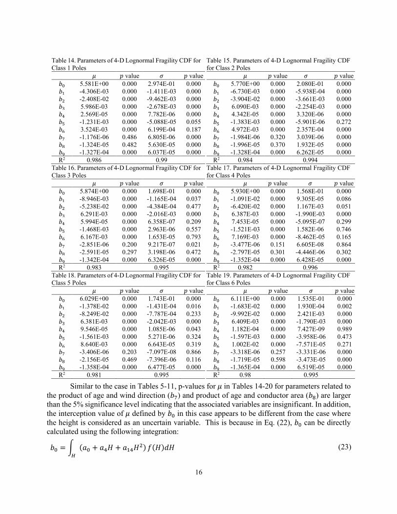
Similar to the case in Tables 5-11, p-values for 𝜇 in Tables 14-20 for parameters related to

the product of age and wind direction (𝑏7) and product of age and conductor area (𝑏8) are larger

than the 5% significance level indicating that the associated variables are insignificant. In addition,

the interception value of 𝜇 defined by 𝑏0 in this case appears to be different from the case where

the height is considered as an uncertain variable. This is because in Eq. (22), 𝑏0 can be directly

calculated using the following integration:

𝑏0 = ∫ (𝑎0 + 𝑎4𝐻 + 𝑎14𝐻2)𝐻

𝑓(𝐻)𝑑𝐻 (23)

Table 15. Parameters of 4-D Lognormal Fragility CDF

for Class 2 Poles 𝜇 𝑝 value 𝜎 𝑝 value

𝑏0 5.770E+00 0.000 2.080E-01 0.000

𝑏1 -6.730E-03 0.000 -5.938E-04 0.000

𝑏2 -3.904E-02 0.000 -3.661E-03 0.000

𝑏3 6.090E-03 0.000 -2.254E-03 0.000

𝑏4 4.342E-05 0.000 3.320E-06 0.000

𝑏5 -1.383E-03 0.000 -5.901E-06 0.272

𝑏6 4.972E-03 0.000 2.357E-04 0.000

𝑏7 -1.984E-06 0.320 3.039E-06 0.000

𝑏8 -1.996E-05 0.370 1.932E-05 0.000

𝑏9 -1.328E-04 0.000 6.262E-05 0.000

R2 0.984 0.994

Table 17. Parameters of 4-D Lognormal Fragility CDF

for Class 4 Poles 𝜇 𝑝 value 𝜎 𝑝 value

𝑏0 5.930E+00 0.000 1.568E-01 0.000

𝑏1 -1.091E-02 0.000 9.305E-05 0.086

𝑏2 -6.420E-02 0.000 1.167E-03 0.051

𝑏3 6.387E-03 0.000 -1.990E-03 0.000

𝑏4 7.453E-05 0.000 -5.095E-07 0.299

𝑏5 -1.521E-03 0.000 1.582E-06 0.746

𝑏6 7.169E-03 0.000 -8.462E-05 0.165

𝑏7 -3.477E-06 0.151 6.605E-08 0.864

𝑏8 -2.797E-05 0.301 -4.446E-06 0.302

𝑏9 -1.352E-04 0.000 6.428E-05 0.000

R2 0.982 0.996

Table 19. Parameters of 4-D Lognormal Fragility CDF

for Class 6 Poles 𝜇 𝑝 value 𝜎 𝑝 value

𝑏0 6.111E+00 0.000 1.535E-01 0.000

𝑏1 -1.683E-02 0.000 1.930E-04 0.002

𝑏2 -9.992E-02 0.000 2.421E-03 0.000

𝑏3 6.409E-03 0.000 -1.790E-03 0.000

𝑏4 1.182E-04 0.000 7.427E-09 0.989

𝑏5 -1.597E-03 0.000 -3.958E-06 0.473

𝑏6 1.002E-02 0.000 -7.571E-05 0.271

𝑏7 -3.318E-06 0.257 -3.331E-06 0.000

𝑏8 -1.719E-05 0.598 -3.473E-05 0.000

𝑏9 -1.365E-04 0.000 6.519E-05 0.000

R2 0.98 0.995

Table 14. Parameters of 4-D Lognormal Fragility CDF for

Class 1 Poles 𝜇 𝑝 value 𝜎 𝑝 value

𝑏0 5.581E+00 0.000 2.974E-01 0.000

𝑏1 -4.306E-03 0.000 -1.411E-03 0.000

𝑏2 -2.408E-02 0.000 -9.462E-03 0.000

𝑏3 5.986E-03 0.000 -2.678E-03 0.000

𝑏4 2.569E-05 0.000 7.782E-06 0.000

𝑏5 -1.231E-03 0.000 -5.088E-05 0.055

𝑏6 3.524E-03 0.000 6.199E-04 0.187

𝑏7 -1.176E-06 0.486 6.805E-06 0.000

𝑏8 -1.324E-05 0.482 5.630E-05 0.000

𝑏9 -1.327E-04 0.000 6.037E-05 0.000

R2 0.986 0.99

Table 16. Parameters of 4-D Lognormal Fragility CDF for

Class 3 Poles 𝜇 𝑝 value 𝜎 𝑝 value

𝑏0 5.874E+00 0.000 1.698E-01 0.000

𝑏1 -8.946E-03 0.000 -1.165E-04 0.037

𝑏2 -5.238E-02 0.000 -4.384E-04 0.477

𝑏3 6.291E-03 0.000 -2.016E-03 0.000

𝑏4 5.994E-05 0.000 6.358E-07 0.209

𝑏5 -1.468E-03 0.000 2.963E-06 0.557

𝑏6 6.167E-03 0.000 1.653E-05 0.793

𝑏7 -2.851E-06 0.200 9.217E-07 0.021

𝑏8 -2.591E-05 0.297 3.198E-06 0.472

𝑏9 -1.342E-04 0.000 6.326E-05 0.000

R2 0.983 0.995

Table 18. Parameters of 4-D Lognormal Fragility CDF for

Class 5 Poles 𝜇 𝑝 value 𝜎 𝑝 value

𝑏0 6.029E+00 0.000 1.743E-01 0.000

𝑏1 -1.378E-02 0.000 -1.431E-04 0.016

𝑏2 -8.249E-02 0.000 -7.787E-04 0.233

𝑏3 6.381E-03 0.000 -2.042E-03 0.000

𝑏4 9.546E-05 0.000 1.085E-06 0.043

𝑏5 -1.561E-03 0.000 5.271E-06 0.324

𝑏6 8.640E-03 0.000 6.643E-05 0.319

𝑏7 -3.406E-06 0.203 -7.097E-08 0.866

𝑏8 -2.156E-05 0.469 -7.396E-06 0.116

𝑏9 -1.358E-04 0.000 6.477E-05 0.000

R2 0.981 0.995

17

Therefore, the interception in the two cases are different. Similarly, the coefficients of the first and

second power of age, wind direction and conductor area are different in Eqs. (19) and (22) as the

coefficients in Eq. (22) can be directly obtained from Eq. (19) by an integration over height (𝐻).

3.3. Investigating the impact of design parameters on the fragility of poles

The fragility models provided in Eqs. (18-19) and (21-22) can be easily used along with Tables 5-

11 and 14-20 to estimate the probability of failure of individual wood poles in distribution

networks. Impacts of covariates including class, age, and conductor area, among others, on the

fragility of wood poles (whose coefficients are defined through parameters, 𝑎𝑖 in Tables 5-11 and

𝑏𝑖 in Tables 14-20) are further investigated in this section.

As a strengthening strategy in power distribution networks, vulnerable poles can be replaced

with lower classes (Salman et al., 2015). This is because the circumference of poles increases as

the class number decreases. The wind-induced moment demand on poles is a direct function of the

circumference, while moment capacity is a function of circumference to power 2.68 (𝑀𝑅 =

Σ𝑅 . 𝐶𝑔𝑙3

32. 𝜋2⁄ =

𝐴. 𝐶𝑔𝑙−0.32. 𝐶𝑔𝑙

3

32. 𝜋2⁄ ). Therefore, it is expected that the probability of failure of poles

is smaller for lower classes of poles. To investigate this effect, fragility curves for different classes

of poles are generated for the set of design parameters presented in Table 12. These fragilities are

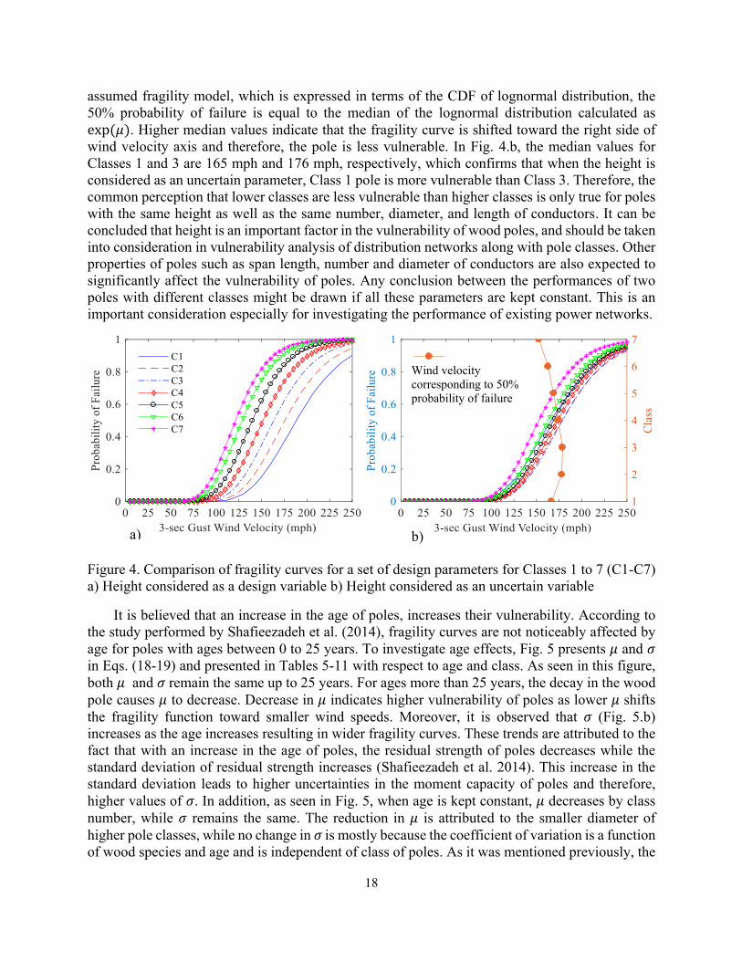
shown in Fig. 4.a. It is seen that as the class number decreases, the vulnerability of poles decreases.

For example, for the wind speed of 150 mph, the probability of failure for Classes 1 to 7 are 0.15,

0.24, 0.35, 0.48, 0.62, 0.75, and 0.82, respectively. It should be mentioned that this comparison is

made assuming that the height as well as other design parameters are the same for all poles in these

classes. In distribution lines, however, lower pole classes are also used when higher clearances are

needed. This is confirmed by results in Table 3 where the mean height of lower classes is higher.

Therefore, if the height is considered as an uncertain parameter, there may be cases where lower

classes are more vulnerable than higher pole classes. To investigate the impact of height

uncertainty on the vulnerability of poles, a set of fragility curves are generated for Classes 1

through 7 for the design parameters presented in Table 21. Results (Fig. 4.b.) show that since the

height of Class 1 poles is considerably higher than other classes, the vulnerability of this class is

more than Classes 2 through 4. However, for classes that have closer heights, such as Classes 5

through 7, the vulnerability increases as the class number increases. For example, for a wind speed

of 150 mph, the probability of failure for design parameters presented in Table 21, for Classes 1

through 7 is 0.34, 0.23, 0.22, 0.26, 0.30, 0.36, and 0.47, respectively. In addition, Fig. 4.b. provides

the wind speed corresponding to 50% probability of failure as a function of class of pole. For the

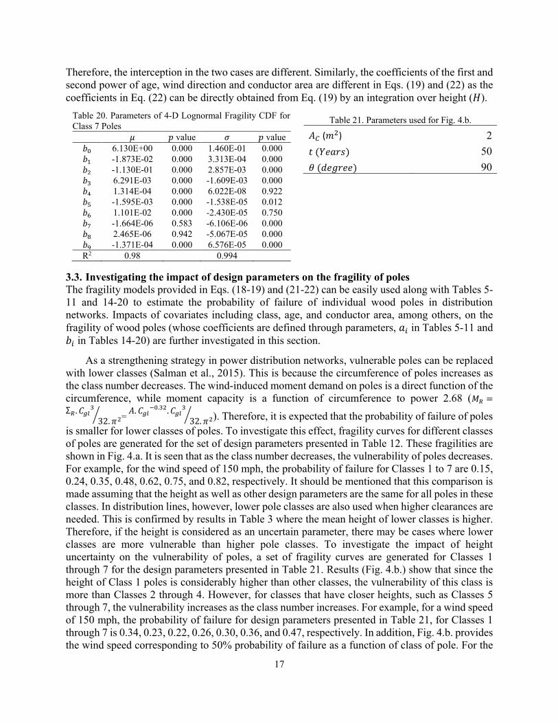
Table 21. Parameters used for Fig. 4.b.

𝐴𝐶 (𝑚2) 2

𝑡 (𝑌𝑒𝑎𝑟𝑠) 50

𝜃 (𝑑𝑒𝑔𝑟𝑒𝑒) 90

Table 20. Parameters of 4-D Lognormal Fragility CDF for

Class 7 Poles 𝜇 𝑝 value 𝜎 𝑝 value

𝑏0 6.130E+00 0.000 1.460E-01 0.000

𝑏1 -1.873E-02 0.000 3.313E-04 0.000

𝑏2 -1.130E-01 0.000 2.857E-03 0.000

𝑏3 6.291E-03 0.000 -1.609E-03 0.000

𝑏4 1.314E-04 0.000 6.022E-08 0.922

𝑏5 -1.595E-03 0.000 -1.538E-05 0.012

𝑏6 1.101E-02 0.000 -2.430E-05 0.750

𝑏7 -1.664E-06 0.583 -6.106E-06 0.000

𝑏8 2.465E-06 0.942 -5.067E-05 0.000

𝑏9 -1.371E-04 0.000 6.576E-05 0.000

R2 0.98 0.994

18

assumed fragility model, which is expressed in terms of the CDF of lognormal distribution, the

50% probability of failure is equal to the median of the lognormal distribution calculated as

exp(𝜇). Higher median values indicate that the fragility curve is shifted toward the right side of

wind velocity axis and therefore, the pole is less vulnerable. In Fig. 4.b, the median values for

Classes 1 and 3 are 165 mph and 176 mph, respectively, which confirms that when the height is

considered as an uncertain parameter, Class 1 pole is more vulnerable than Class 3. Therefore, the

common perception that lower classes are less vulnerable than higher classes is only true for poles

with the same height as well as the same number, diameter, and length of conductors. It can be

concluded that height is an important factor in the vulnerability of wood poles, and should be taken

into consideration in vulnerability analysis of distribution networks along with pole classes. Other

properties of poles such as span length, number and diameter of conductors are also expected to

significantly affect the vulnerability of poles. Any conclusion between the performances of two

poles with different classes might be drawn if all these parameters are kept constant. This is an

important consideration especially for investigating the performance of existing power networks.

Figure 4. Comparison of fragility curves for a set of design parameters for Classes 1 to 7 (C1-C7)

a) Height considered as a design variable b) Height considered as an uncertain variable

It is believed that an increase in the age of poles, increases their vulnerability. According to

the study performed by Shafieezadeh et al. (2014), fragility curves are not noticeably affected by

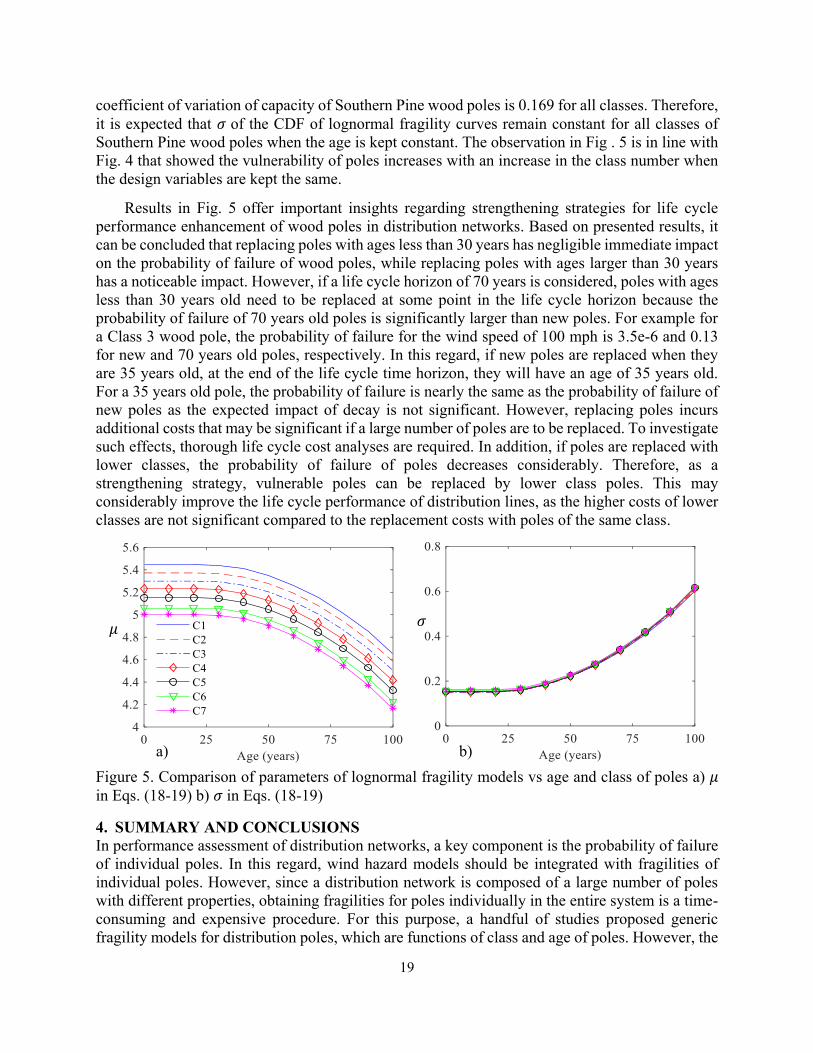
age for poles with ages between 0 to 25 years. To investigate age effects, Fig. 5 presents 𝜇 and 𝜎

in Eqs. (18-19) and presented in Tables 5-11 with respect to age and class. As seen in this figure,

both 𝜇 and 𝜎 remain the same up to 25 years. For ages more than 25 years, the decay in the wood

pole causes 𝜇 to decrease. Decrease in 𝜇 indicates higher vulnerability of poles as lower 𝜇 shifts

the fragility function toward smaller wind speeds. Moreover, it is observed that 𝜎 (Fig. 5.b)

increases as the age increases resulting in wider fragility curves. These trends are attributed to the

fact that with an increase in the age of poles, the residual strength of poles decreases while the

standard deviation of residual strength increases (Shafieezadeh et al. 2014). This increase in the

standard deviation leads to higher uncertainties in the moment capacity of poles and therefore,

higher values of 𝜎. In addition, as seen in Fig. 5, when age is kept constant, 𝜇 decreases by class

number, while 𝜎 remains the same. The reduction in 𝜇 is attributed to the smaller diameter of

higher pole classes, while no change in 𝜎 is mostly because the coefficient of variation is a function

of wood species and age and is independent of class of poles. As it was mentioned previously, the

a) b)

Wind velocity

corresponding to 50%

probability of failure

(median) for each class

19

coefficient of variation of capacity of Southern Pine wood poles is 0.169 for all classes. Therefore,

it is expected that 𝜎 of the CDF of lognormal fragility curves remain constant for all classes of

Southern Pine wood poles when the age is kept constant. The observation in Fig . 5 is in line with

Fig. 4 that showed the vulnerability of poles increases with an increase in the class number when

the design variables are kept the same.

Results in Fig. 5 offer important insights regarding strengthening strategies for life cycle

performance enhancement of wood poles in distribution networks. Based on presented results, it

can be concluded that replacing poles with ages less than 30 years has negligible immediate impact

on the probability of failure of wood poles, while replacing poles with ages larger than 30 years

has a noticeable impact. However, if a life cycle horizon of 70 years is considered, poles with ages

less than 30 years old need to be replaced at some point in the life cycle horizon because the

probability of failure of 70 years old poles is significantly larger than new poles. For example for

a Class 3 wood pole, the probability of failure for the wind speed of 100 mph is 3.5e-6 and 0.13

for new and 70 years old poles, respectively. In this regard, if new poles are replaced when they

are 35 years old, at the end of the life cycle time horizon, they will have an age of 35 years old.

For a 35 years old pole, the probability of failure is nearly the same as the probability of failure of

new poles as the expected impact of decay is not significant. However, replacing poles incurs

additional costs that may be significant if a large number of poles are to be replaced. To investigate

such effects, thorough life cycle cost analyses are required. In addition, if poles are replaced with

lower classes, the probability of failure of poles decreases considerably. Therefore, as a

strengthening strategy, vulnerable poles can be replaced by lower class poles. This may

considerably improve the life cycle performance of distribution lines, as the higher costs of lower

classes are not significant compared to the replacement costs with poles of the same class.

Figure 5. Comparison of parameters of lognormal fragility models vs age and class of poles a) 𝜇

in Eqs. (18-19) b) 𝜎 in Eqs. (18-19)

4. SUMMARY AND CONCLUSIONS

In performance assessment of distribution networks, a key component is the probability of failure

of individual poles. In this regard, wind hazard models should be integrated with fragilities of

individual poles. However, since a distribution network is composed of a large number of poles

with different properties, obtaining fragilities for poles individually in the entire system is a time-

consuming and expensive procedure. For this purpose, a handful of studies proposed generic

fragility models for distribution poles, which are functions of class and age of poles. However, the

a) b)

𝜇 𝜎

20

wind performance of poles depends on a larger set of parameters. For example, span length,

diameter and number of conductors, and wind direction can considerably impact the probability of

failure of wood poles.

In order to address the aforementioned limitations, the current study, for the first time,

develops multi-dimensional wind fragility models for utility wood poles. These models account

for a comprehensive set of design parameters including class, height, and age of wood poles, wind

direction, and number, diameter, and length of conductors. The fragility models are obtained by

fitting a response surface to the fragility parameters obtained from 1000 realizations of design

variables. In this regard, for each set of design variables, a fragility curve is generated through

derivation of failure probabilities for a wide range of wind speeds. The Lognormal CDF model is

found to provide a good fit to empirical fragility results. The parameters of the fitted lognormal

CDFs are recorded and used as training points to develop response surface models based on a

Generalized Linear Model (GLM). GLMs consider interactions among different design parameters

as well as their high order powers. The produced GLMs provide simple and accurate models for

the fragility of wood poles. Results indicate that, if height of poles remains constant, the fragility

of poles increases when the class number increases. Moreover, the fragility of pole does not

significantly change with an increase in the age of poles when age is less than 30 years old while

it noticeably decreases when age is more than 30 years old. Furthermore, if the height of poles in

each class is considered as an uncertain variable rather than a design parameter, lower classes of

poles may not always be more reliable than higher classes. Particularly, it is observed that since

the height of poles in Class 1 is considerably larger than other classes, they are more vulnerable

than poles in Classes 2 through 4, if height is considered uncertain. On the other hand since Classes

5 through 7 poles have closer heights, the vulnerability of poles increases as the class number

increases. Probabilistic models used for a number of input variables in this study are derived based

on a large database of Southern Yellow Pine wood poles in the US for Classes 1 through 7. The

produced multi-dimensional fragility models can be used for risk analysis of distribution networks

made of Southern Yellow Pines in the US or regions with similar poles and climate conditions.

The proposed fragility models help researchers, engineers, planners, and more broadly,

stakeholders of power distribution systems investigate the performance of existing distribution

lines, evaluate various replacement options, and therefore, choose the most cost effective

hardening alternative through a life cycle cost analysis. For this purpose, the proposed fragility

models can be integrated with wind hazard models to estimate the annual probability of failure of

poles in distribution networks and generate failure scenarios for the system. Using network

analysis procedures, these failure scenarios can then predict power outages in the distribution

network. Estimating power outages can yield the incurred hazard cost due to revenue and economic

losses. Extending the annual incurred hazard costs along with mitigation and maintenance costs to

the life cycle time horizon of a distribution network provide insights about the benefits of various

retrofit alternatives and helps in decision making processes as the retrofit option with the least total

life cycle cost is the most favorable one.

ACKNOWLEDGEMENT

This paper is based upon work supported by the National Science Foundation under Grants No.

CMMI- 1333943 and 1635569. This support is greatly appreciated.

REFERENCES

ANSI O5.1, Specifications and Dimensions for Wood Poles, Amer. Nat. Std. Inst. (ANSI), New

York, 2008.

21

ASCE (American Society of Civil Engineers) (2010), “Minimum design loads for buildings and

other structures”. Standard ASCE/SEI 7-10.Reston, VA, USA;

ASCE No. 74 (2009) “Guidelines for Electrical Transmission Line Structural Loading” American

Society of Civil Engineers.

Bhat R., Y. Mohammadi Darestani, A. Shafieezadeh, A.P. Meliopoulos, R. DesRoches.

“Resilience Assessment of Distribution Systems Considering the Effect of Hurricanes”, IEEE

PES Transmission and Distribution Conference & Exposition. Denver, Co. USA. April 16-

19, 2018

Brown, R. E., in IEEE GM 2006 Working Group on System Design, Jun. 21, 2006. [Online].

Available: http://grouper.ieee.org/groups/td/dist/sd/doc/2006-06-Hurricane-Wilma.pdf

Darestani, Y. M., and A. Shafieezadeh. "Modeling the Impact of Adjacent Spans in Overhead

Distribution Lines on the Wind Response of Utility Poles." In Geotechnical and Structural

Engineering Congress 2016a, pp. 1067-1077.

Darestani, Y.M , A. Shafieezadeh, and R. DesRoches. "An equivalent boundary model for effects

of adjacent spans on wind reliability of wood utility poles in overhead distribution lines."

Engineering Structures 128 2016b: 441-452.

Darestani, Y. M., A. Shafieezadeh, and R. DesRoches. "Effects of Adjacent Spans and Correlated

Failure Events on System-Level Hurricane Reliability of Power Distribution Lines." IEEE

Transactions on Power Delivery 2017.

Darestani, Y. M., and A. Shafieezadeh, “Hurricane Performance Assessment of Power Distribution

Lines Using Multi-scale Matrix-based System Reliability Analysis Method”, 13th Americas

Conference on Wind Engineering, Gainesville, Florida, USA, May 21 - 24, 2017

Ellingwood, B. R., and P. B. Tekie. "Wind load statistics for probability-based structural design."

Journal of Structural Engineering 125, no. 4: 453-463, 1999.

Ellingwood, B. R., D.V. Rosowsky, Y. Li, and J. H. Kim. "Fragility assessment of light-frame

wood construction subjected to wind and earthquake hazards." Journal of Structural

Engineering 130, no. 12 (2004): 1921-1930.

Ebad-Sichani, M., J. E. Padgett, and V. Bisadi. "Probabilistic seismic analysis of concrete dry cask

structures." Structural Safety 73 2018: pp 87-98.

Fereshtehnejad, E., M. Banazadeh, and A. Shafieezadeh. (2016):"System reliability-based seismic

collapse assessment of steel moment frames using incremental dynamic analysis and Bayesian

probability network." Engineering Structures 118 :274-286.

Ghosh, J., J. E. Padgett, and L. Dueñas-Osorio. "Surrogate modeling and failure surface

visualization for efficient seismic vulnerability assessment of highway bridges." Probabilistic

Engineering Mechanics 34 (2013): pp.189-199.

Ghosh, J., and J. E. Padgett. "Aging considerations in the development of time-dependent seismic

fragility curves." Journal of Structural Engineering 136, no. 12 (2010): 1497-1511.

Ibach, R. E. "Wood preservation." Wood handbook: wood as an engineering material. Madison,

WI: USDA Forest Service, Forest Products Laboratory, 1999. General technical report FPL;

GTR-113: Pages 14.1-14.27 113.

Johnson, B., "Utility storm restoration response." Edison Electric Institute, Washington DC., 2004.

L. Kocis and W. Whiten, “Computational investigations of low-discrepancy sequences,” vol. 23,

no.2, pp. 266–294, 1997.

Lacaze S. and S. Missoum (2015). "CODES: A Toolbox For Computational Design". Version 1.0.

URL: www.codes.arizona.edu/toolbox.

22

Li, Y., S. Yeddanapudi, J. D. McCalley, A. A. Chowdhury, and M. Moorehead. "Degradation-path

model for wood pole asset management." In Power Symposium, Proceedings of the 37th

Annual North American, pp. 275-280. IEEE, 2005.

Li, Y., and B. R. Ellingwood. "Hurricane damage to residential construction in the US: Importance

of uncertainty modeling in risk assessment." Engineering structures 28, no. 7 (2006): 1009-

1018.

Onyewuchi, U. P., A. Shafieezadeh, M. M. Begovic, and R. DesRoches. "A Probabilistic

Framework for Prioritizing Wood Pole Inspections Given Pole Geospatial Data." Smart Grid,

IEEE Transactions on 6, no. 2: 973-979, 2015.

Ryan, P. C., M. G. Stewart, N. Spencer, and Y. Li. "Reliability assessment of power pole

infrastructure incorporating deterioration and network maintenance." Reliability Engineering

& System Safety 132 (2014): 261-273.

Reed, D. A., C. J. Friedland, S. Wang, and C. C. Massarra. "Multi-hazard system-level logit

fragility functions." Engineering Structures 122 (2016): 14-23.lo

Salman, A. M., Y. Li, and M. G. Stewart. "Evaluating system reliability and targeted hardening

strategies of power distribution systems subjected to hurricanes." Reliability Engineering &

System Safety 144: 319-333, 2015.

Sandoz, J. L., and O. Vanackere. "Wood poles ageing and non destructive testing tool.", 14th

International Conference and Exhibition on Electricity Distribution (Distributing Power for

the Millennium), 1997 : v3-26.

Shafieezadeh, A., U. P. Onyewuchi, M. M. Begovic, and R. DesRoches. "Age-dependent fragility

models of utility wood poles in power distribution networks against extreme wind hazards."

Power Delivery, IEEE Transactions on 29, no. 1: 131-139, 2014.

Shinozuka, M., M. Q. Feng, J. Lee, and T. Naganuma. "Statistical analysis of fragility curves."

Journal of engineering mechanics 126, no. 12 (2000): 1224-1231.

Van de Lindt, J. W., and T. N. Dao. "Performance-based wind engineering for wood-frame

buildings." Journal of Structural Engineering 135, no. 2 , 2009: 169-177.

Wang, Z. and Shafieezadeh, A., 2019. REAK: Reliability analysis through Error rate-based

Adaptive Kriging. Reliability Engineering & System Safety, 182, pp.33-45.

Wolfe, R. W., J. Bodig, and P. Lebow. "Derivation of nominal strength for wood utility poles.",

U.S. Dept. Agriculture, Forest Service, Forest Products Lab., Madison, WI, USA, Rep. FPL-

GTR-128, 2001.