Progress In Electromagnetics Research B, Vol. 25, 241–259, 2010 MULTI-FLOOR INDOOR POSITIONING SYSTEM USING BAYESIAN GRAPHICAL MODELS A. S. Al-Ahmadi, A. I. Omer, M. R. Kamarudin and T. A. Rahman Wireless Communication Centre Universiti Teknologi Malaysia Skudai, Johor 81310, Malaysia Abstract—In recent years, location determination systems have gained a high importance due to their rule in the context aware systems. In this paper, we will design a multi-floor indoor positioning system based on Bayesian Graphical Models (BGM). Graphical models have a great flexibility on visualizing the relationships between random variables. Rather than using one sampling technique, we are going to use multiple sets each set contains a collection of sampling techniques, the accuracy of each set will be compared with each other. 1. INTRODUCTION Recent advances in communication technologies have a great impact on location determination systems. Location determination systems are deployed in almost every building, from hospitals were the location of patients and doctors or any medical equipment can be determined, or sending information to customers based on their location, to organize the traffic and reducing congestion in the highways. RADAR [1] is an in-building RF-based user location and tracking system uses the nearest neighbor in signal space (NNSS) technique to predict the user’s location. NNSS uses the online received signal strength (RSS) to search for the closest match stored in the radio map during the offline phase by minimizing the Euclidean distance between the physical location of the user and the estimated location. The system depends on empirical data collection to build a radio map for the test bed. The radio map contains tuples in the form Received 12 August 2010, Accepted 7 September 2010, Scheduled 14 September 2010 Corresponding author: A. S. Al-Ahmadi ([email protected]).
Transcript
Progress In Electromagnetics Research B, Vol. 25, 241–259, 2010
A. S. Al-Ahmadi, A. I. Omer, M. R. Kamarudinand T. A. Rahman
Wireless Communication CentreUniversiti Teknologi MalaysiaSkudai, Johor 81310, Malaysia
Abstract—In recent years, location determination systems havegained a high importance due to their rule in the context awaresystems. In this paper, we will design a multi-floor indoor positioningsystem based on Bayesian Graphical Models (BGM). Graphical modelshave a great flexibility on visualizing the relationships between randomvariables. Rather than using one sampling technique, we are going touse multiple sets each set contains a collection of sampling techniques,the accuracy of each set will be compared with each other.
1. INTRODUCTION
Recent advances in communication technologies have a great impact onlocation determination systems. Location determination systems aredeployed in almost every building, from hospitals were the location ofpatients and doctors or any medical equipment can be determined, orsending information to customers based on their location, to organizethe traffic and reducing congestion in the highways.
RADAR [1] is an in-building RF-based user location and trackingsystem uses the nearest neighbor in signal space (NNSS) techniqueto predict the user’s location. NNSS uses the online received signalstrength (RSS) to search for the closest match stored in the radiomap during the offline phase by minimizing the Euclidean distancebetween the physical location of the user and the estimated location.The system depends on empirical data collection to build a radiomap for the test bed. The radio map contains tuples in the form
Received 12 August 2010, Accepted 7 September 2010, Scheduled 14 September 2010Corresponding author: A. S. Al-Ahmadi ([email protected]).
242 Al-Ahmadi et al.
(t, x, y, d) where t represents the timestamp, (x, y) is the coordinatesof user’s location and d is the orientation of the user’s facing (north,south, east or west). RADAR’s accuracy is effected by the size ofNNSS used, training points and samples size in the online phase.The system also uses signal propagation modeling approach to buildthe radio map, the goal was to reduce the system dependence onempirical data. The authors ignored the Floor Attenuation Factor(FAF) which was proposed by [2] and adopted the Wall AttenuationFactor (WAF) instead. They discovered that there is an inverserelationship between the amount of additional attenuation and thenumber of walls separating the transmitter and the receiver. Theaccuracy of the system was about 2–3 m.
Horus [3], a probabilistic WLAN location determination systemwhich was designed with the goal of high accuracy and lowcomputational cost. The system uses a technique called location-clustering in order to reduce the computational cost. Having asmall computational cost systems is an important aspect in designinga location determination system, it enables such systems to beimplemented in smaller devices. The system also operates in twostages: an Off-line phase where the radio map is built using a JointClustering technique where the test bed is divided into clusters, andany two locations are in the same cluster if they are both covered bythe same APs, a discrete space estimator estimates the RSS histogramfor each AP at each location, and an On-line phase, where the actualestimating of the user’s location happen by finding the location xwhich maximize the probability of getting that location given a signalstrength vector s.
In [4], the authors presented a hybrid indoor positioning methodthat uses ray-tracing model for modeling the multipath effects. Thesystem works in two stages, in the first stage, it uses the direction ofarrival (DOA) and RSS to build a database of fingerprints, while inthe second stage it determines the position of the mobile station bycomputing the Euclidean distance values of DOA and RSS with thevalues stored in the database.
In [5], the authors proposed an indoor location determinationsystem that uses non line of sight (NLOS) scheme and one boundscattering paths. The system is a two step Determination and Selection(two step DS), which in the first step it calculates the estimatedlocation from a cluster of Line of Possible Mobile Device location(LPMD). In the second step, the system tries to find the shortestEuclidean distance from the centroid. The system adjusts the Lineof Sight (LOS) measurement of the Angle of Arrival (AOA) and TOAto the real values.
Progress In Electromagnetics Research B, Vol. 25, 2010 243
The disadvantage of the above systems is that they do not workin multi-floor environments. Most indoor positioning system based onTOA or AOA metrics requires a sophisticated devices to measure timeor angle. Since our system was designed to work with off-the-shelfcomponents, which means no additional requirements were neededother than an Access Point (AP) and a WiFi enabled device. Moreover,TOA location determination systems uses the TOA measurement ofthe first path to determine the location which in turn is difficult to becalculated accurately in indoor environments [6].
For a list of systems and methods used in indoor locationdetermination [7–10].
2. RSS PROPERTIES IN INDOOR ENVIRONMENTS
In order for us to design an ideal indoor positioning system, studyingthe properties of RSS in indoor environments is a crucial aspect in thisstudy. Signal strength in indoor environments is difficult to predict dueto multipath effects such as reflection, diffraction and scattering [11].In this section, we are going to study different RSS properties that willeffect our system.
2.1. Distribution of RSS in Indoor Environment
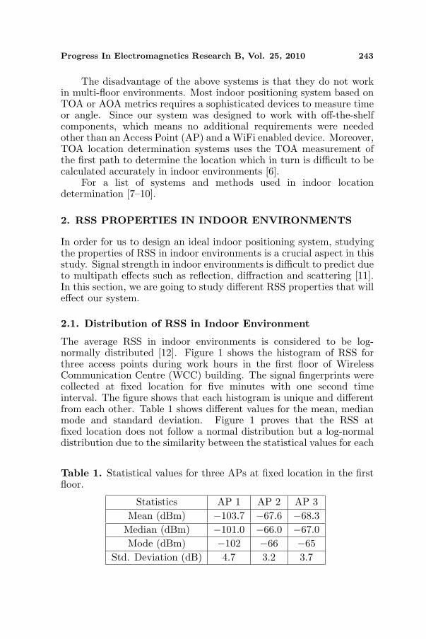
The average RSS in indoor environments is considered to be log-normally distributed [12]. Figure 1 shows the histogram of RSS forthree access points during work hours in the first floor of WirelessCommunication Centre (WCC) building. The signal fingerprints werecollected at fixed location for five minutes with one second timeinterval. The figure shows that each histogram is unique and differentfrom each other. Table 1 shows different values for the mean, medianmode and standard deviation. Figure 1 proves that the RSS atfixed location does not follow a normal distribution but a log-normaldistribution due to the similarity between the statistical values for each
Table 1. Statistical values for three APs at fixed location in the firstfloor.
Statistics AP 1 AP 2 AP 3Mean (dBm) −103.7 −67.6 −68.3
Median (dBm) −101.0 −66.0 −67.0Mode (dBm) −102 −66 −65
Std. Deviation (dB) 4.7 3.2 3.7
244 Al-Ahmadi et al.
Figure 1. RSS distribution at fixed locations from three access points.
AP. Moreover, the data did not pass D’Agostino-Pearson Omnibus testsince the P values for each test were too small.
2.2. Using RSS to Infer Locations
In our system, RSS will be used as reference to infer the indoor location.A test was conducted to show the possibility of using RSS, Figure 2shows the variation of RSS measurements recorded from five APs whilewalking through a track in the first floor at WCC building. The signalreceived at any given location is higher when that location is close tothe AP, and weaker when it is far away. This shows the feasibility ofusing RSS as a location fingerprint.
Figure 2 also shows the uniqueness of RSS tuples. Each RSS tuplesat each location are different. This indicates that RSS fingerprints arethe best choice for inferring indoor locations. The figure shows alsothe small variation of RSS against the distance which indicates thedistance between each training point should not be relatively small.
Progress In Electromagnetics Research B, Vol. 25, 2010 245
Figure 2. RSS while walking inside WCC from five APs.
Table 2. RSSs statistics from two APs at two different floors.
Min −57.00 −76.00 −82.00 −51.00Max −43.00 −69.00 −46.00 −44.00
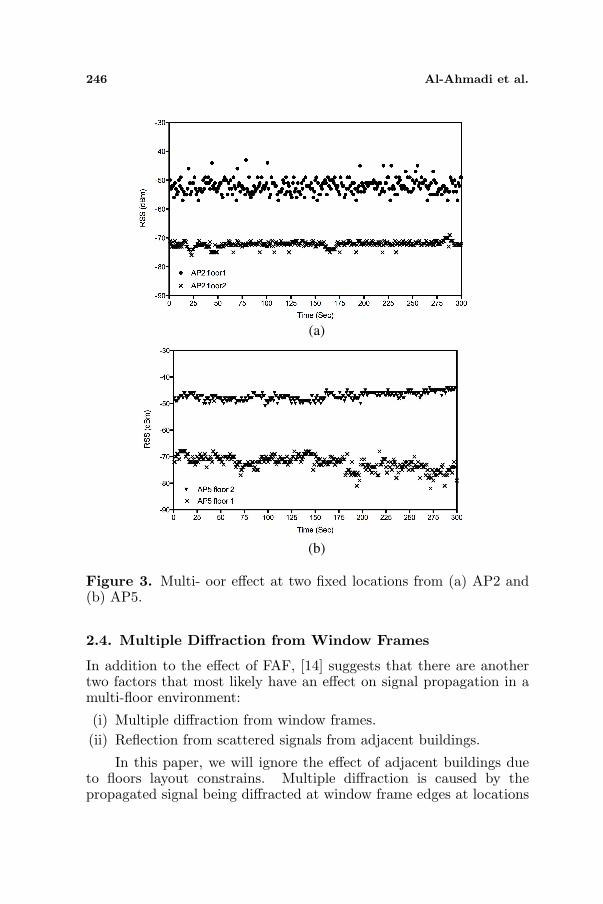
2.3. Multi-floor Effect
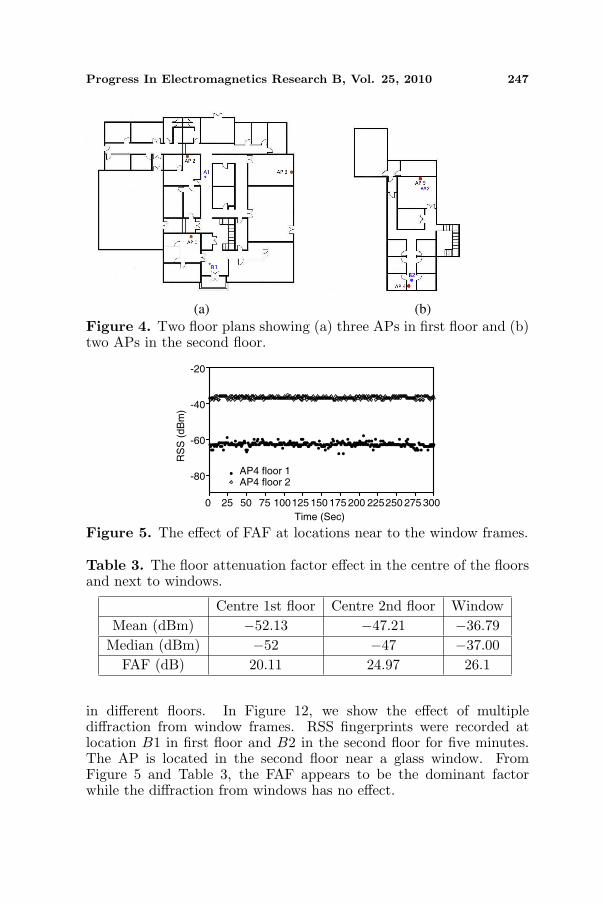
According to [13], a concrete floor may reduce the RSS between15 dB and 35 dB. In order to investigate the effect of floors in theindoor environment, we performed a set of measurements at two fixedlocations referred as A1 in Figure 4(a) and A2 in Figure 4(b), A1 andA2 are vertically and symmetrical locations.
At each location, we have collected RSSs for five minutes with1 second sampling time from AP2 in first floor and AP5 in the secondfloor.
Figure 3 and Table 2 show the effect of floor in our test bed, forAP2 the floor attenuation is 20.11 dB and 24.97 dB for AP5. Theaverage floor attenuation to the RSS from an AP implemented indifferent floor is 22.5 dB.
246 Al-Ahmadi et al.
(b)
(a)
Figure 3. Multi- oor effect at two fixed locations from (a) AP2 and(b) AP5.
2.4. Multiple Diffraction from Window Frames
In addition to the effect of FAF, [14] suggests that there are anothertwo factors that most likely have an effect on signal propagation in amulti-floor environment:
(i) Multiple diffraction from window frames.(ii) Reflection from scattered signals from adjacent buildings.
In this paper, we will ignore the effect of adjacent buildings dueto floors layout constrains. Multiple diffraction is caused by thepropagated signal being diffracted at window frame edges at locations
Progress In Electromagnetics Research B, Vol. 25, 2010 247
(a) (b)
Figure 4. Two floor plans showing (a) three APs in first floor and (b)two APs in the second floor.
0 25 50 75 100125 150 175 200 225250 275 300
-80
-60
-40
-20
AP4 floor 1AP4 floor 2
Time (Sec)
RS
S (
dB
m)
Figure 5. The effect of FAF at locations near to the window frames.
Table 3. The floor attenuation factor effect in the centre of the floorsand next to windows.
Centre 1st floor Centre 2nd floor WindowMean (dBm) −52.13 −47.21 −36.79
Median (dBm) −52 −47 −37.00FAF (dB) 20.11 24.97 26.1
in different floors. In Figure 12, we show the effect of multiplediffraction from window frames. RSS fingerprints were recorded atlocation B1 in first floor and B2 in the second floor for five minutes.The AP is located in the second floor near a glass window. FromFigure 5 and Table 3, the FAF appears to be the dominant factorwhile the diffraction from windows has no effect.
248 Al-Ahmadi et al.
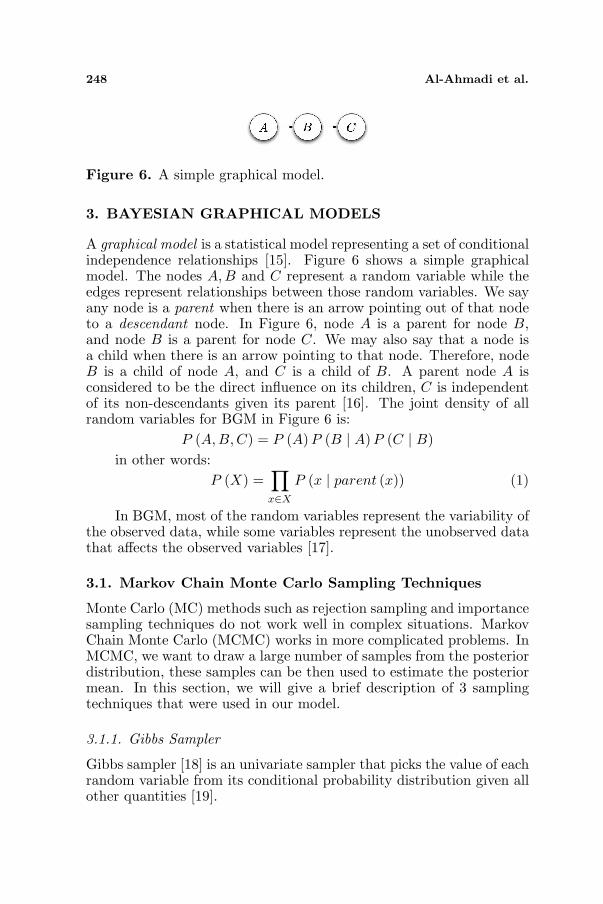
Figure 6. A simple graphical model.
3. BAYESIAN GRAPHICAL MODELS
A graphical model is a statistical model representing a set of conditionalindependence relationships [15]. Figure 6 shows a simple graphicalmodel. The nodes A,B and C represent a random variable while theedges represent relationships between those random variables. We sayany node is a parent when there is an arrow pointing out of that nodeto a descendant node. In Figure 6, node A is a parent for node B,and node B is a parent for node C. We may also say that a node isa child when there is an arrow pointing to that node. Therefore, nodeB is a child of node A, and C is a child of B. A parent node A isconsidered to be the direct influence on its children, C is independentof its non-descendants given its parent [16]. The joint density of allrandom variables for BGM in Figure 6 is:
P (A, B,C) = P (A) P (B | A) P (C | B)in other words:
P (X) =∏
x∈X
P (x | parent (x)) (1)
In BGM, most of the random variables represent the variability ofthe observed data, while some variables represent the unobserved datathat affects the observed variables [17].
3.1. Markov Chain Monte Carlo Sampling Techniques
Monte Carlo (MC) methods such as rejection sampling and importancesampling techniques do not work well in complex situations. MarkovChain Monte Carlo (MCMC) works in more complicated problems. InMCMC, we want to draw a large number of samples from the posteriordistribution, these samples can be then used to estimate the posteriormean. In this section, we will give a brief description of 3 samplingtechniques that were used in our model.
3.1.1. Gibbs Sampler
Gibbs sampler [18] is an univariate sampler that picks the value of eachrandom variable from its conditional probability distribution given allother quantities [19].
Progress In Electromagnetics Research B, Vol. 25, 2010 249
If we have a simple regression model:si ∼ N (b0 + b1X1 + . . . + bzXz, τ) (2)
the Gibbs sampler works by sampling each of the conditionaldistribution one at a time, Algorithm 1 shows the steps of Gibbssampler [20]:
Algorithm 1 The Gibbs Sampler algorithm(i) Set initial values for parameters bi
Metropolis-Hasting was initiated by [21] as a generalization of theMetropolis algorithm which was introduced by [22]. Algorithm 2 showsthe steps of a Metropolis-Hasting algorithm.
Algorithm 2 Metropolis-Hasting algorithm(i) Set initial values for parameters bi
(ii) For t = 1, . . . , T repeat(a) Set b = b(t−1)
(b) Generate new value b′ from a proposal distribution h (b′|b)(c) Calculate
α = min(
1,f (b′|S) h (b|b′)f (b|S) h (b′|b)
)
(d) Update b(t) = b′ with probability α, otherwise set b(t) = b
250 Al-Ahmadi et al.
3.1.3. Slice Sampler
Slice sampling [23] works by using a supportive variable v, and drawingsamples from the joint distribution Uniform (b, v) such that:
p (b, v) ={
1/B if 0 ≤ v ≤ p (x)0 otherwise
(4)
where B =∫
p (b) db, and the marginal distribution over b is:
p (b) =∫
p (b) dv =∫ p(b)
0
1B
dv (5)
Algorithm 3 Slice Sampler Algorithm(i) Set b = b(t−1)
(ii) For i = 1, . . . , n
(a) generate v(t)i ∼ Uniform (0, f (vi|b))
(iii) For j = 1, . . . , d
(a) update bj ∼ f (bj)∏n
i=1 I(0 ≤ v
(t)i ≤ f (vi|b)
)
(iv) Set b(t) = b
3.2. Burn-in Samples
Burn-in samples are samples that were initially generated and will berejected in order to eliminate their effect on the posterior distribution,burn-in samples are not valid since Markov chain has not stabilized [20].
3.3. Ordered Over-relaxation
Over-relaxation [24] is used to improve the convergence of Gibbssampler, it generates multiple random values at each iteration andchooses the one that is negatively correlated with the current valuefrom a conditional distribution and then arranging these values in non-decreasing order.
4. MODEL AND MEASUREMENT SETUP
A single unshaded circle symbolizes a continuous stochastic node whilethe shaded node represents a discrete stochastic node, stochastic nodesare always assigned to a distribution, discrete stochastic nodes are
Progress In Electromagnetics Research B, Vol. 25, 2010 251
represented by a single shaded circle, while a double unshaded circlerefers to a logical variable, and finally, single rectangular represents aconstant.
4.1. Data Collection
In order to construct a radio map for our test bed, an offline datacollection at specified locations was needed. NetStumbler [25], a freesoftware for detecting signal strengths from APs was used. In additionto RSSs, NetStumbler can also record MAC, SSID, SNR and channelspeed of each AP. Unfortunately, due to experiencing some difficultieswith NetStumbler, like the inability to record the location of thefingerprint collected and not being able to operate in some operatingsystems, we developed UTM WiFi Scanner, a software that allowsus to record RSSs, MAC address, SSID, channel and speed of eachAPs along with their (x, y) coordinates and z (the floor number). Oursoftware is based on inSSIDer [26], an open source WLAN scannerwritten in C sharp language under Apache license.
We performed our test at WCC building at UTM, the buildinghas two floors, first floor is about 36 m× 30 m and the second floor isapproximately 21 m× 28m, there are five D-Link DWL-2000AP APs,with operating frequency from 2.4GHz to 2.4835 GHz, 3 in the firstfloor and 2 in the second floor, each AP has 15 dBm transmit power.Most of the building’s walls are concrete and some walls are made ofa plaster partition board, the wall thickness is about 15 cm and floorthickness is about 80 cm, Figure 4 show the building’s floor plan. RSSsfingerprints were collected on a MacBook running Windows XP ServicePack 3 in Boot Camp. The laptop is equipped with AirPort Extremecard, the card supports IEEE 802.11 a/b/g/n standards.
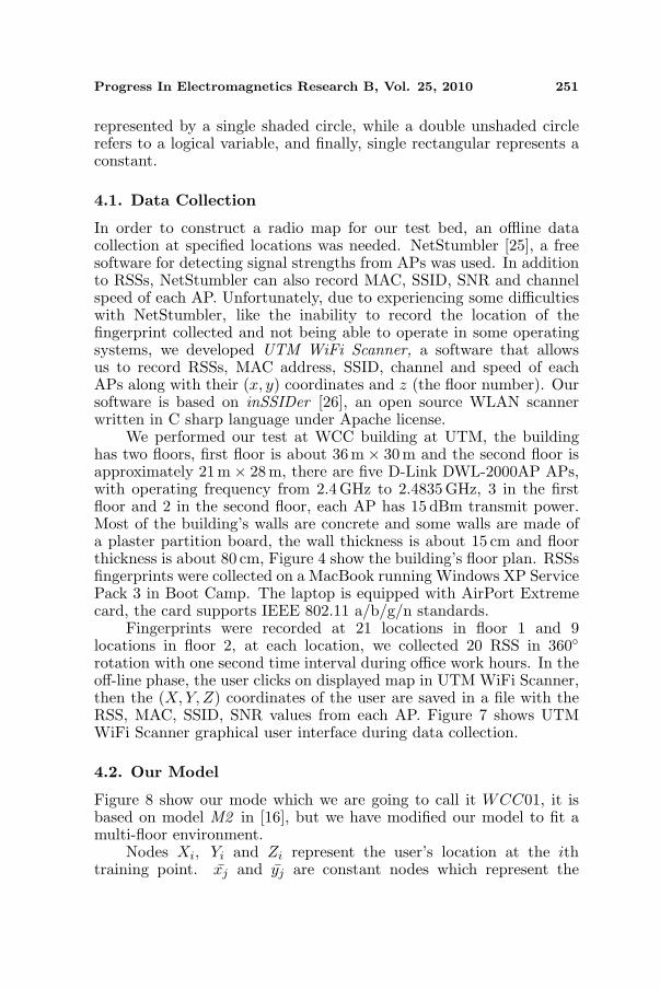
Fingerprints were recorded at 21 locations in floor 1 and 9locations in floor 2, at each location, we collected 20 RSS in 360◦rotation with one second time interval during office work hours. In theoff-line phase, the user clicks on displayed map in UTM WiFi Scanner,then the (X,Y, Z) coordinates of the user are saved in a file with theRSS, MAC, SSID, SNR values from each AP. Figure 7 shows UTMWiFi Scanner graphical user interface during data collection.
4.2. Our Model
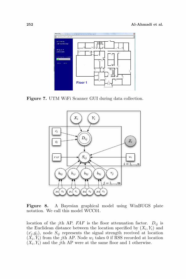
Figure 8 show our mode which we are going to call it WCC01, it isbased on model M2 in [16], but we have modified our model to fit amulti-floor environment.
Nodes Xi, Yi and Zi represent the user’s location at the ithtraining point. xj and yj are constant nodes which represent the
252 Al-Ahmadi et al.
Figure 7. UTM WiFi Scanner GUI during data collection.
Figure 8. A Bayesian graphical model using WinBUGS platenotation. We call this model WCC01.
location of the jth AP. FAF is the floor attenuation factor. Dij isthe Euclidean distance between the location specified by (Xi, Yi) and(xj ,yj), node Sij represents the signal strength received at location(Xi, Yi) from the jth AP. Node wi takes 0 if RSS recorded at location(Xi, Yi) and the jth AP were at the same floor and 1 otherwise.
Progress In Electromagnetics Research B, Vol. 25, 2010 253
The nodes are defined as follows:
Xi ∼ U (0, L)Yi ∼ U (0,W )Zi ∼ DisU (1, N)
Dij = log(
1 +√
(Xi − xj)2 + (Yi − yj)
2
)
Sij ∼ Norm(b0j + (b1j ∗Dij ) + (b2j ∗ Zi)+(b3j ∗ wi ∗ FAF ), τj), i = 1, . . . , n,
j = 1, . . . , m,
bcj ∼ Norm (µc, τc) , c = 1, 2, 3, 4,
µc ∼ Norm (0, 1.0E − 6) , c = 1, 2, 3, 4,
τc ∼ Gamma (0.01, 0.01) , c = 1, 2, 3, 4.
L represents the length of the test bed while W is the width and N isthe number of floors.
Since WinBUGS (Bayesian Inference Using Gibbs Sampler) doesnot support discrete uniform distribution, we had to construct our owndistribution as a categorical distribution as follows:
for (i in 1 : 30) {p[i] < −30 Z[i] ∼ dcat(p[ ])}Categorical distribution is a generalization of Bernoulli distribu-
tion with sample space {1, 2, 3, . . . , n}. It can be used in BUGS by:
x ∼ dcat(p[ ]) (6)
wherex = 1, 2, 3, . . . , dim(p)
4.3. Data Analysis
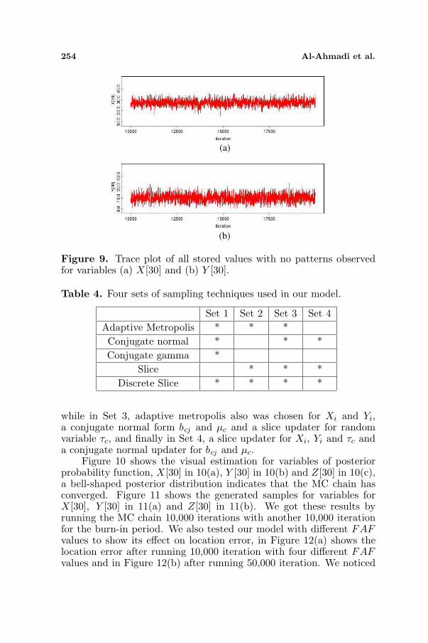
In order to compute the posterior distribution, we will use BUGS [27],a free software used to generate samples for the parameters of posteriordistribution. Figure 9 shows two trace plots for Xi in Figure 9(a) andfor Yi in Figure 9(b), clearly the two random variables Xi and Yi haveconverged since no patterns were observed, then we do not have togenerate more samples.
We simulate using four sets of sampling methods as appear inTable 4. In Set 1, adaptive metropolis updater was used for randomvariables Xi and Yi, a discrete slice updater was chosen for Zi in thefour steps, conjugate normal updater for bcj and µc, and a conjugategamma updater for random variable τc. In Set 2, adaptive metropolisupdater was used for Xi, Yi, bcj and µc and a slice updater for τc,
254 Al-Ahmadi et al.
(a)
(b)
Figure 9. Trace plot of all stored values with no patterns observedfor variables (a) X[30] and (b) Y [30].
Table 4. Four sets of sampling techniques used in our model.
Set 1 Set 2 Set 3 Set 4Adaptive Metropolis * * *Conjugate normal * * *Conjugate gamma *
Slice * * *Discrete Slice * * * *
while in Set 3, adaptive metropolis also was chosen for Xi and Yi,a conjugate normal form bcj and µc and a slice updater for randomvariable τc, and finally in Set 4, a slice updater for Xi, Yi and τc anda conjugate normal updater for bcj and µc.
Figure 10 shows the visual estimation for variables of posteriorprobability function, X[30] in 10(a), Y [30] in 10(b) and Z[30] in 10(c),a bell-shaped posterior distribution indicates that the MC chain hasconverged. Figure 11 shows the generated samples for variables forX[30], Y [30] in 11(a) and Z[30] in 11(b). We got these results byrunning the MC chain 10,000 iterations with another 10,000 iterationfor the burn-in period. We also tested our model with different FAFvalues to show its effect on location error, in Figure 12(a) shows thelocation error after running 10,000 iteration with four different FAFvalues and in Figure 12(b) after running 50,000 iteration. We noticed
Progress In Electromagnetics Research B, Vol. 25, 2010 255
(a) (b)
(c)
Figure 10. An approximate visual kernel estimate of the posteriordistribution of random variables (a) X[30], (b) Y [30] and (c) Z[30].
(a) (b)
Figure 11. Generated samples using Gibbs sampler for (a) X[30],Y [30] and (b) Z[30].
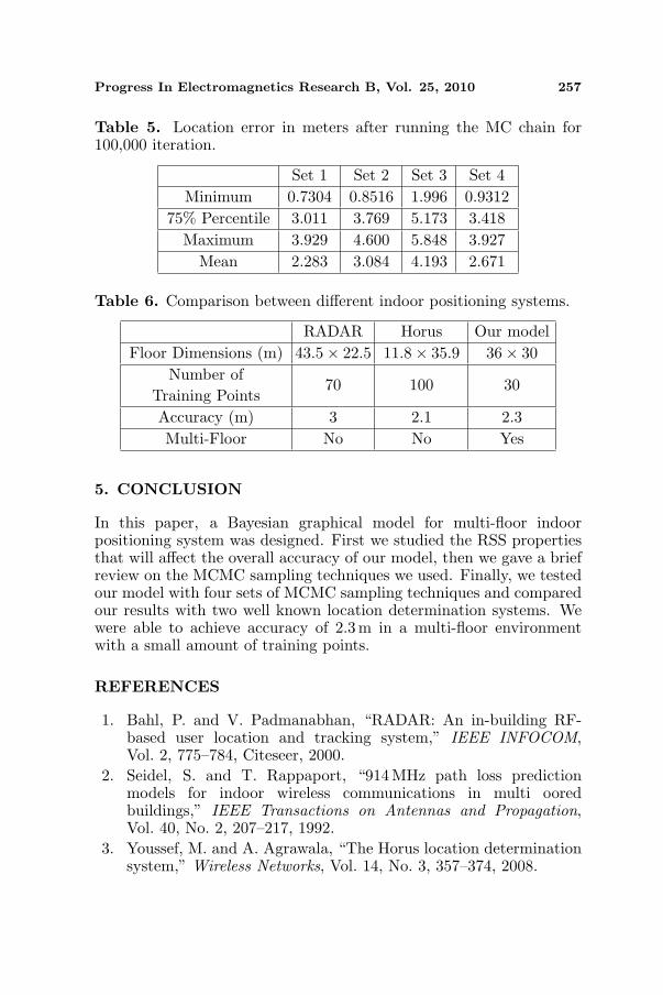
that the overall accuracy was increased while the number of iterationsincreased. We got better results with FAF = 25 dB, the error mean atthis value is about 3.8 m. In Figure 13, we show our results with eachsets mention in Table 4 after choosing FAF = 25 dB, we ran the MCchain for 100,000 iteration after discarding the first 10,000 iteration asburn-in samples. From Table 5, Set 1 of sampling techniques appears
256 Al-Ahmadi et al.
(a) (b)
Figure 12. The effect of different FAF values and number ofiterations on the estimated location error.
Set 1
0
2
4
6
8 100,000 Iteration
Err
or
(m)
Set 2
Set 3
Set 4
Figure 13. Location error results using the four sets with FAF =25dB after running the MC chain for 100,000 iteration and 10,000iteration in burn-in period.
to give the most accurate results with mean error of 2.283m and 75%percentile of 3 meters, while Set 3 gives the most inaccurate results byerror mean of about 4.2 m and 75% percentile equal to 5.17 m.
In Table 6, we compare our results with similar off-the-shelfpositioning systems, namely RADAR [1] and the Horus locationdetermination system proposed by [3]. Although the dimensions ofthe first floor of our test bed is bigger than the test bed in [3], wewere able to achieve almost the same accuracy with 70% less trainingpoints. Note that our 30 training points were collected in two floors.
Progress In Electromagnetics Research B, Vol. 25, 2010 257
Table 5. Location error in meters after running the MC chain for100,000 iteration.
Set 1 Set 2 Set 3 Set 4Minimum 0.7304 0.8516 1.996 0.9312
In this paper, a Bayesian graphical model for multi-floor indoorpositioning system was designed. First we studied the RSS propertiesthat will affect the overall accuracy of our model, then we gave a briefreview on the MCMC sampling techniques we used. Finally, we testedour model with four sets of MCMC sampling techniques and comparedour results with two well known location determination systems. Wewere able to achieve accuracy of 2.3m in a multi-floor environmentwith a small amount of training points.
REFERENCES
1. Bahl, P. and V. Padmanabhan, “RADAR: An in-building RF-based user location and tracking system,” IEEE INFOCOM,Vol. 2, 775–784, Citeseer, 2000.
2. Seidel, S. and T. Rappaport, “914 MHz path loss predictionmodels for indoor wireless communications in multi ooredbuildings,” IEEE Transactions on Antennas and Propagation,Vol. 40, No. 2, 207–217, 1992.
3. Youssef, M. and A. Agrawala, “The Horus location determinationsystem,” Wireless Networks, Vol. 14, No. 3, 357–374, 2008.
258 Al-Ahmadi et al.
4. Tayebi, A., J. Gomez, F. Saez de Adana, and O. Gutierrez,“The application of ray-tracing to mobile localization using thedirection of arrival and received signal strength in multipathindoor environments,” Progress In Electromagnetics Research,Vol. 91, 1–15, 2009.
5. Seow, C. and S. Tan, “Localization of omni-directional mobiledevice in multipath environments,” Progress In ElectromagneticsResearch, Vol. 85, 323–348, 2008.
6. Kanaan, M. and K. Pahlavan, “A comparison of wirelessgeolocation algorithms in the indoor environment,” IEEE WirelessCommunications and Networking Conference, 177–182, 2004.
7. Honkavirta, V., T. Perala, S. Ali-Loytty, and R. Piche, “Acomparative survey of WLAN location fingerprinting methods,”6th Workshop on Positioning, Navigation and CommunicationWPNC, 2009.
8. Liu, H., H. Darabi, P. Banerjee, and J. Liu, “Survey of wirelessindoor positioning techniques and systems,” IEEE Transactionson Systems, Man, and Cybernetics, Part C: Applications andReviews, Vol. 37, No. 6, 1067–1080, 2007.
9. Pandey, S. and P. Agrawal, “A survey on localization techniquesfor wireless networks,” Journal — Chinese Institute of Engineers,Vol. 29, No. 7, 1125, 2006.
10. Wallbaum, M. and S. Diepolder, “Benchmarking wirelesslan location systems,” Proceedings of the 2005 Second IEEEInternational Workshop on Mobile Commerce and Services(WMCS 2005), 42–51, Munich, Germany, 2005.
11. Pahlavan, K. and P. Krishnamurthy, Principles of WirelessNetworks, Prentice Hall PTR, New Jersey, 2002.
12. Kaemarungsi, K. and P. Krishnamurthy, “Properties of indoorreceived signal strength for WLAN location fingerprinting,”Proceedings of the 1st Annual International Conference onMobile and Ubiquitous Systems: Networking and Services(MOBIQUITOUS04), 14–23, 2004.
13. Komar, C. and C. Ersoy, “Location tracking and location basedservice using IEEE 802.11 WLAN infrastructure,” EuropeanWireless, 24–27, 2004.
14. Tan, S., M. Tan, and H. Tan, “Multipath delay measurementsand modeling for inter floor wireless communications,” IEEETransactions on Vehicular Technology, Vol. 49, No. 4, 1334–1341,Jul. 2000.
15. Jensen, F., “Bayesian graphical models,” Encyclopedia of
Progress In Electromagnetics Research B, Vol. 25, 2010 259
Environmetrics, 2000.16. Elnahrawy, E., R. Martin, W. Ju, P. Krishnan, and D. Madigan,
17. Noble, W., “Getting started in probabilistic graphical models,”PLoS Comput. Biol., Vol. 3, No. 12, 252, 2007.
18. Geman, S., D. Geman, K. Abend, T. Harley, and L. Kanal,“Stochastic relaxation, Gibbs distributions and the Bayesianrestoration of images*,” Journal of Applied Statistics, Vol. 20,No. 5, 25–62, 1993.
19. Cowles, M., “Review of WinBUGS 1.4,” The AmericanStatistician, Vol. 58, No. 4, 330–336, 2004.
20. Ntzoufras, I., Bayesian Modeling Using WinBUGS, John Wiley &Sons Inc, 2009.
21. Hastings, W., “Monte Carlo sampling methods using Markovchains and their applications,” Biometrika, Vol. 57, No. 1, 97–109, 1970.
22. Metropolis, N., A. Rosenbluth, M. Rosenbluth, A. Teller,E. Teller, et al., “Equation of state calculations by fast computingmachines,” The Journal of Chemical Physics, Vol. 21, No. 6, 1087,1953.
23. Neal, R., “Slice sampling,” Annals of Statistics, Vol. 31, No. 3,705–741, 2003.
24. Neal, R. M., “Suppressing random walks in Markov chainMonte Carlo using ordered overrelaxation,” Learning in GraphicalModels, 205–225, 1998.