Multi-Fluid MHD Simulation of FRC Translation

E.T. Meier, V.S. Lukin, R. Milroy, U. Shumlak,

Plasma Science and Innovation CenterUniversity of Washington

ICCJune 24-27, 2008

Resources used:• PSI-Center SGI Altix 350 cluster• NERSC IBM p575 POWER 5 system, BassiThis research is funded by DOE.

• SEL overview• FRC translation problem• Visco-resistive MHD model 1

+ Atomic physics 2+ Spitzer / Chodura variable resistivity 3+ Two-fluid effects

• SEL-NIMROD results comparison– MHD with uniform resistivity

• Comparison of SEL results with 1 , 2 , and 3 • Future work

Outline

SEL overview

• 2D high-order spectral elements– Crucial for modeling extreme anisotropies of

laboratory fusion plasmas.• Flux-source form and modular programming

– Allows straightforward implementation of a wide variety of physics models.

• Fully implicit time advance

*Ref. ICC 2008 poster by V.S. Lukin – E10

SEL – Spectral ELement code*

FRC translation problem

Initial condition is generated by a separate equilibrium solver.

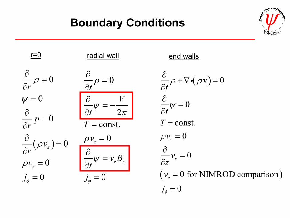
• FRC translation is a valuable code development problem.– Various boundary conditions are necessary.– High gradients and velocities test code capability.

Normalization

0ψψ ψ= 4

0 3.9 10 Wbψ −= ×

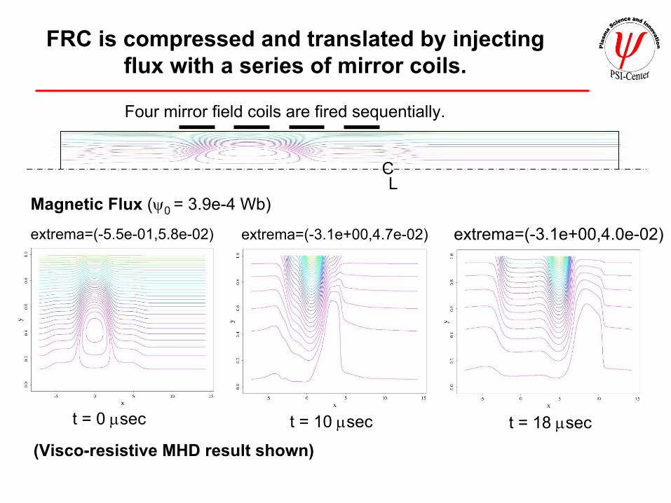
FRC is compressed and translated by injecting flux with a series of mirror coils.

CL

Four mirror field coils are fired sequentially.

t = 0 µsec t = 10 µsec t = 18 µsec

Magnetic Flux (ψ0 = 3.9e-4 Wb)

extrema=(-5.5e-01,5.8e-02) extrema=(-3.1e+00,4.7e-02) extrema=(-3.1e+00,4.0e-02)

(Visco-resistive MHD result shown)

Visco-resistive MHD model

Visco-resistive MHD model

( ) 2Dtρ ρ ρ∂+∇ = ∇

∂vi

( )r jt φψ η φ∂ = − × ∂

v B i

( )

( )

// //

2

11 1

:

p p T Tt

p jφ

γ κ κ κγ γ

η µ

⊥ ⊥

∂+∇ − − ∇ + ∇ − ∂ −

= ∇ + + ∇ ∇ + ∇

v

v v v v

i

i T

( ) ( )2

02Bp

tρ

ρ µ ∂ +∇ + + − − ∇ + ∇ = ∂

vvv I BB v vi T

( ) ˆjφ φ= ∇×B i where

1 1ˆ ˆ, r zr z r r

ψ ψ∂ ∂= −

∂ ∂B , ˆ ˆ, r zv r v z=v ,

and axisymmetry is assumed ( 0φ∇ → ).

Density diffusion is needed when resolution is

insufficient.

This model only allows for toroidal current.

( )rAφψ = −

Boundary Conditions

( )

0

0

0

0

00

z

r

r

pr

vrvjφ

ρ

ψ

ρ

ρ

∂=

∂=

∂=

∂∂

=∂

==

r=0 radial wall end walls

( )

( )

0

0

const.0

0

0 for NIMROD comparison0

z

r

r

t

tTv

vzvjφ

ρ ρ

ψ

ρ

∂+∇ =

∂∂

=∂==

∂=

∂=

=

vi0

2const.

0

0

z

r z

tV

tTv

v Btjφ

ρ

ψπ

ρ

ψ

∂=

∂∂

= −∂==

∂=

∂=

+ atomic physics

Atomic physics model, I.C., and B.C.

( ) .2

.ion recombDtρ ρ ρ +∂+∇ = ∇ Γ −

∂Γvi

2. .

nn ion recombD

tρ ρ∂

= ∇ −Γ +Γ∂

( )r jt φψ η φ∂ = − × ∂

v B i

( ) . . .1 ... ...

11

1ion i ion recomb ip m mt

pγ ργ

−Γ Φ − Γ

∂+∇ =

− ∂ − i

( ) ( ) .... recomb itm

ρ−

∂+∇

∂Γ= v

vi

( ) ˆjφ φ= ∇×B i

where .ionΦ is the specific ionization potential.

. .ion ion e i nn nσΓ = ⟨ ⟩v , 2. .recomb recomb e inσΓ = ⟨ ⟩v 1/ 213

, 3 -1

, ,

2 10 13.6exp m s6.0 /13.6 13.6

e eVion e

e eV e eV

TT T

σ− ×

⟨ ⟩ = − + v

1/ 2

19 3 -1

,

13.60.7 10 m srec ee eVT

σ − ⟨ ⟩ = ×

v .

Ionization and recombination rates for hydrogen*

*Ref. R. J. Goldston, P. H. Rutherford, Introduction to Plasma Physics, IOP Publishing Ltd., 1995

I.C. for neutral density is ( ),max0.1n iρ ρ= .

B.C. for neutral density is . .n

ion recombtρ∂

= −Γ +Γ∂

.

(B.C. for other MHD variables are unchanged.)

Neutral gas is ionized and absorbed by FRC during translation.

Magnetic Flux (ψ0 = 3.9e-4 Wb)

Neutral Density (n0 = 2.5e-7 kg/m3)

t = 0 µsec

t = 9 µsec t = 14 µsec

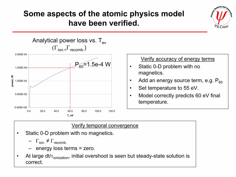
Some aspects of the atomic physics model have been verified.

Verify accuracy of energy terms• Static 0-D problem with no

magnetics.• Add an energy source term, e.g. P60

• Set temperature to 55 eV.• Model correctly predicts 60 eV final

temperature.

Power loss vs. Tev

0.000E+00

5.000E-05

1.000E-04

1.500E-04

2.000E-04

0.0 20.0 40.0 60.0 80.0 100.0 120.0

T, eV

pow

er, W

P60=1.5e-4 W

Analytical power loss vs. Tev(Γion.=Γrecomb.)

Verify temporal convergence• Static 0-D problem with no magnetics.

– Γion. ≠ Γrecomb.

– energy loss terms = zero.• At large dt/τionization, initial overshoot is seen but steady-state solution is

correct.

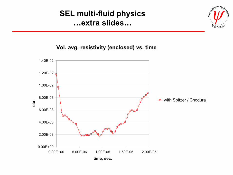
+ Spitzer / Chodura variable resistivity

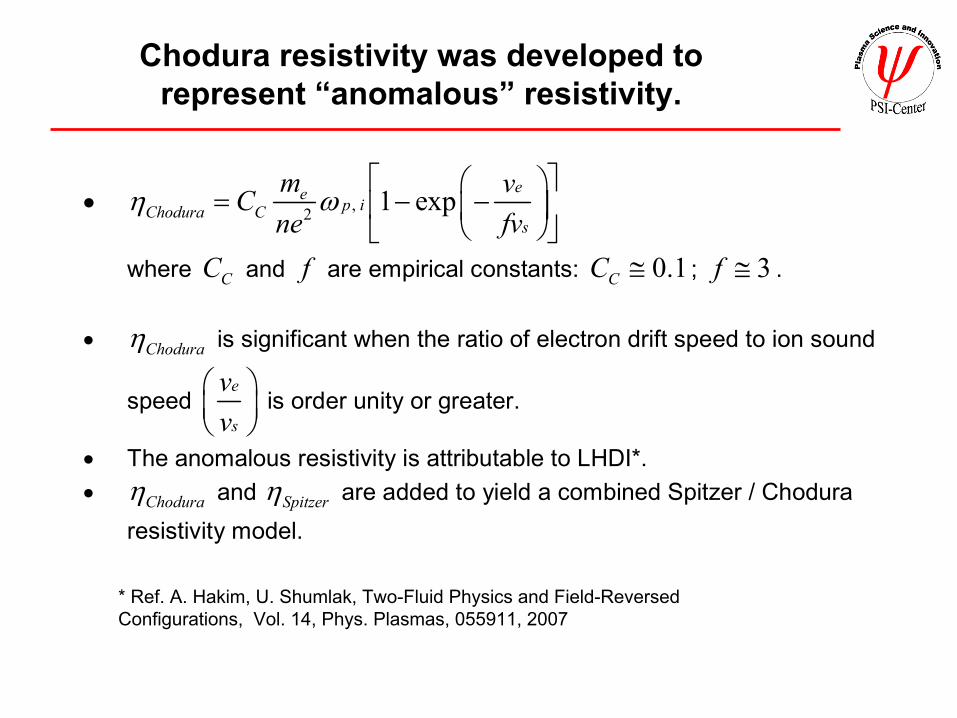
Chodura resistivity was developed to represent “anomalous” resistivity.

• ,2 1 exp eep iChodura C

s

m vCne fv

η ω

= − −

where CC and f are empirical constants: 0.1CC ≅ ; 3f ≅ .

• Choduraη is significant when the ratio of electron drift speed to ion sound

speed e

s

vv

is order unity or greater.

• The anomalous resistivity is attributable to LHDI*. • Choduraη and Spitzerη are added to yield a combined Spitzer / Chodura

resistivity model.

* Ref. A. Hakim, U. Shumlak, Two-Fluid Physics and Field-ReversedConfigurations, Vol. 14, Phys. Plasmas, 055911, 2007

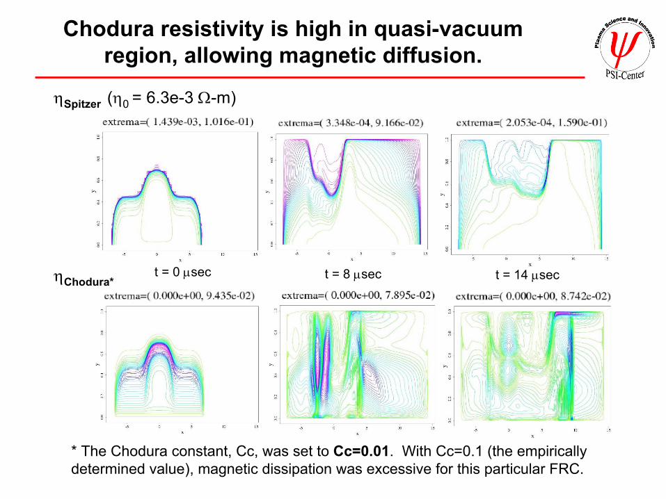
Chodura resistivity is high in quasi-vacuum region, allowing magnetic diffusion.

ηSpitzer (η0 = 6.3e-3 Ω-m)

ηChodura*t = 0 µsec t = 8 µsec t = 14 µsec

* The Chodura constant, Cc, was set to Cc=0.01. With Cc=0.1 (the empirically determined value), magnetic dissipation was excessive for this particular FRC.

+ Two-fluid effects.

Two-fluid MHD model

( ) 2i D

tρ ρ ρ∂+∇ = ∇

∂vi

( )2 ˆie ez e

dr r v z ptψφ φ η ν

ρ ∂ = = − × + ∇ −∇ ∂

E j v Bi i

t∂

= −∇×∂B E

( ) ( ) ( )2

ˆ 02

ii i i i ez

Bp v ztρ

ρ µ ν ∂ +∇ + + − − ∇ + ∇ − ∇ = ∂

vv v I BB v vi T

e i iv v d jφ φ φρ ρ= −

( )

// //

2 2

11 1

:

i

i i i i ez

p p T Tt

p v

γ κ κγ γ

η µ ν

⊥ ⊥

∂+∇ − ∇ − ∇ − ∂ −

= ∇ + + ∇ ∇ + ∇ + ∇

v

v j v v v

i

i T

where

0i

pi

cdLω

= , ˆ ˆ, r zv r v z=v ,

and axisymmetry is assumed ( 0φ∇ → ).

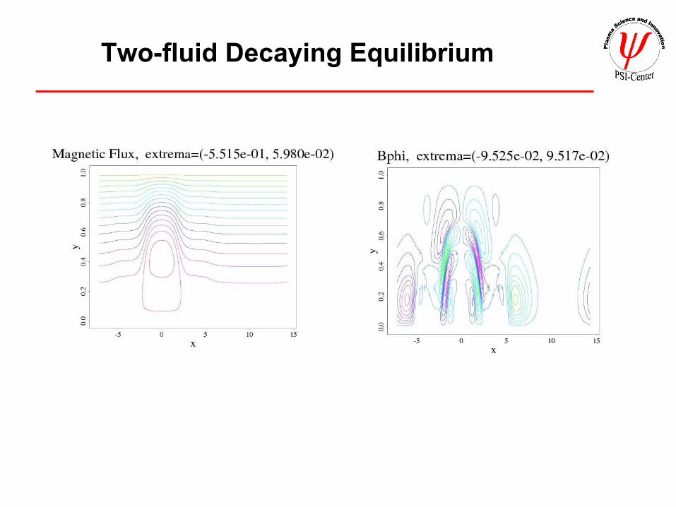
Two-fluid Decaying Equilibrium

SEL-NIMROD comparison(MHD with uniform resistivity)

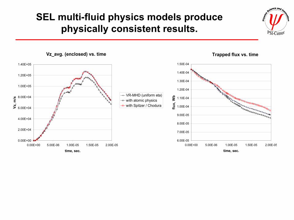
SEL-NIMROD simulations have been run with identical I.C. and parameters.

SEL shows 2.0% lower axial speed at t = 20 µsec.

SEL shows 4.8% less trapped flux at t = 20 µsec.

“Enclosed” refers to the region within the FRC separatrix.

Vz_avg. (enclosed) vs. time

0.00E+00

2.00E+04

4.00E+04

6.00E+04

8.00E+04

1.00E+05

1.20E+05

1.40E+05

0.00E+00 5.00E-06 1.00E-05 1.50E-05 2.00E-05

time, sec.

Vz, m

/s

NIMRODSEL

Trapped flux vs. time

1.00E-04

1.10E-04

1.20E-04

1.30E-04

1.40E-04

1.50E-04

1.60E-04

1.70E-04

1.80E-04

1.90E-04

0.00E+00 5.00E-06 1.00E-05 1.50E-05 2.00E-05

time, sec.

flux,

Wb

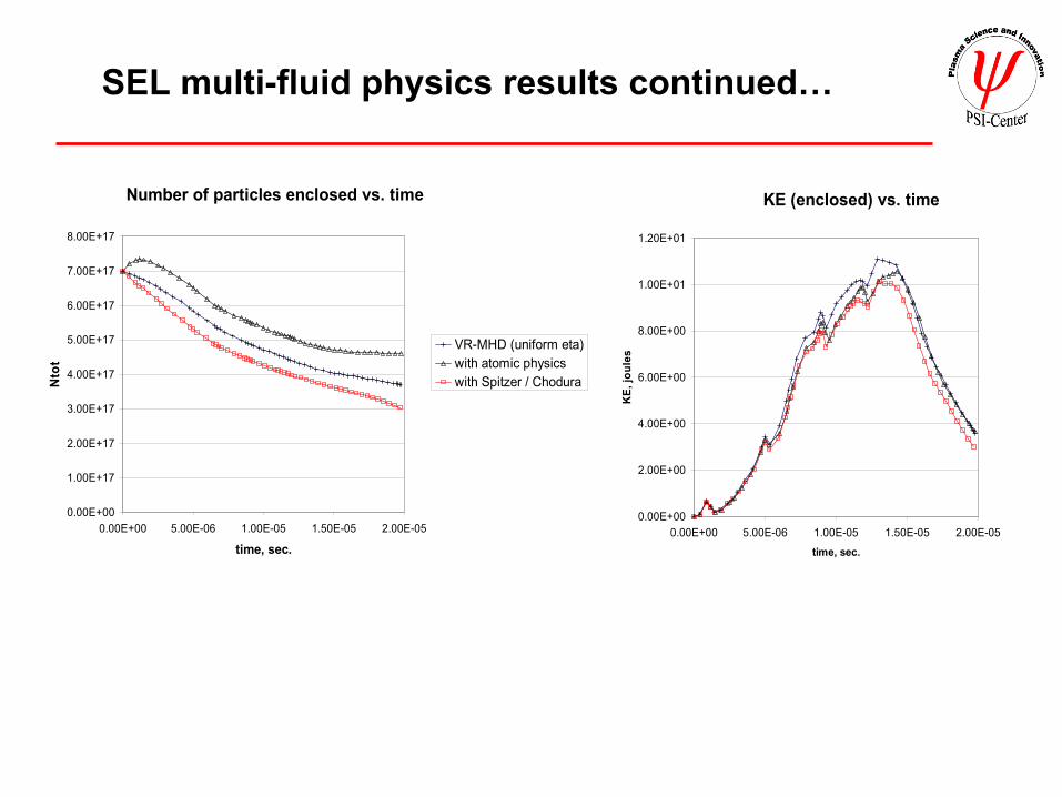
SEL-NIMROD comparison continued…

SEL shows 8.8% less retained particles at t = 20 µsec.

SEL shows 2.3% less KE at t = 20 µsec.

Number of particles enclosed vs. time

4.00E+17

4.50E+17

5.00E+17

5.50E+17

6.00E+17

6.50E+17

7.00E+17

0.00E+00 5.00E-06 1.00E-05 1.50E-05 2.00E-05

time, sec.

Nto

t

NIMRODSEL

KE (enclosed) vs. time

0.00E+00

2.00E+00

4.00E+00

6.00E+00

8.00E+00

1.00E+01

1.20E+01

0.00E+00 5.00E-06 1.00E-05 1.50E-05 2.00E-

time, sec.

KE,

joul

es

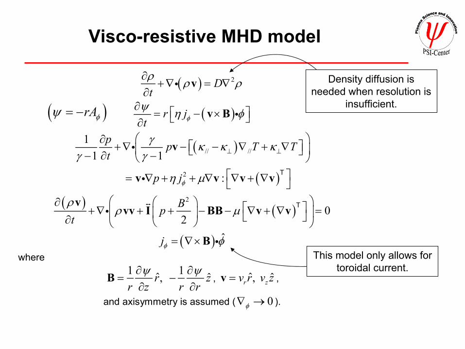
Comparison of SEL results with• Visco-resistive MHD

+ Atomic physics+ Spitzer / Chodura variable resistivity(using Cc=0.01)

SEL multi-fluid physics models produce physically consistent results.

Vz_avg. (enclosed) vs. time

0.00E+00

2.00E+04

4.00E+04

6.00E+04

8.00E+04

1.00E+05

1.20E+05

1.40E+05

0.00E+00 5.00E-06 1.00E-05 1.50E-05 2.00E-05

time, sec.

Vz, m

/s

VR-MHD (uniform eta)with atomic physicswith Spitzer / Chodura

Trapped flux vs. time

6.00E-05

7.00E-05

8.00E-05

9.00E-05

1.00E-04

1.10E-04

1.20E-04

1.30E-04

1.40E-04

1.50E-04

0.00E+00 5.00E-06 1.00E-05 1.50E-05 2.00E-05

time, sec.

flux,

Wb

SEL multi-fluid physics results continued…

Number of particles enclosed vs. time

0.00E+00

1.00E+17

2.00E+17

3.00E+17

4.00E+17

5.00E+17

6.00E+17

7.00E+17

8.00E+17

0.00E+00 5.00E-06 1.00E-05 1.50E-05 2.00E-05

time, sec.

Nto

t

VR-MHD (uniform eta)with atomic physicswith Spitzer / Chodura

KE (enclosed) vs. time

0.00E+00

2.00E+00

4.00E+00

6.00E+00

8.00E+00

1.00E+01

1.20E+01

0.00E+00 5.00E-06 1.00E-05 1.50E-05 2.00E-05

time, sec.

KE,

joul

es

Future Work

• Develop two-fluid MHD modeling via 2D FRC translation simulation.

• Develop and implement more sophisticated boundary conditions.– “open” boundary outflow.– Self-consistent magnetic boundary conditions.– Implement in MHD and for multi-fluid MHD.

• Extend multi-fluid modeling and boundary conditions to 3D.

SEL multi-fluid physics…extra slides…

Vol. averaged beta vs. time

0

1

2

3

4

5

6

0.00E+00 5.00E-06 1.00E-05 1.50E-05 2.00E-05

time, sec.

Bet

a with Spitzer / Chodura

SEL multi-fluid physics…extra slides…

Vol. avg. resistivity (enclosed) vs. time

0.00E+00

2.00E-03

4.00E-03

6.00E-03

8.00E-03

1.00E-02

1.20E-02

1.40E-02

0.00E+00 5.00E-06 1.00E-05 1.50E-05 2.00E-05

time, sec.

eta with Spitzer / Chodura