Louisiana State University LSU Digital Commons LSU Master's eses Graduate School 12-7-2017 Multi-Hazard Performance Assessment of High- Rise Buildings Jad El Khoury Antoun Louisiana State University and Agricultural and Mechanical College, [email protected]Follow this and additional works at: hps://digitalcommons.lsu.edu/gradschool_theses Part of the Civil Engineering Commons , and the Structural Engineering Commons is esis is brought to you for free and open access by the Graduate School at LSU Digital Commons. It has been accepted for inclusion in LSU Master's eses by an authorized graduate school editor of LSU Digital Commons. For more information, please contact [email protected]. Recommended Citation El Khoury Antoun, Jad, "Multi-Hazard Performance Assessment of High-Rise Buildings" (2017). LSU Master's eses. 4368. hps://digitalcommons.lsu.edu/gradschool_theses/4368
Transcript
Louisiana State UniversityLSU Digital Commons
LSU Master's Theses Graduate School
12-7-2017
Multi-Hazard Performance Assessment of High-Rise BuildingsJad El Khoury AntounLouisiana State University and Agricultural and Mechanical College, [email protected]
Follow this and additional works at: https://digitalcommons.lsu.edu/gradschool_theses
Part of the Civil Engineering Commons, and the Structural Engineering Commons
This Thesis is brought to you for free and open access by the Graduate School at LSU Digital Commons. It has been accepted for inclusion in LSUMaster's Theses by an authorized graduate school editor of LSU Digital Commons. For more information, please contact [email protected].
4.1 Description of the structure and location ...........................................................................26 4.2 Details of the steps of the analysis .....................................................................................28
5.1 Seismic loss assessment .....................................................................................................56 5.1.1 Analytical closed-form solution ...............................................................................56 5.1.2 Multilayer Monte Carlo Simulation .........................................................................66
5.2 Wind loss assessment .........................................................................................................72 5.3 Comparison between seismic and wind analysis results ....................................................76
v
6 CONCLUSIONS AND FUTURE WORK ............................................................................78
and (5) loss analysis (see Figure 3.1 and Figure 3.2). Hence, a five-fold integration was used to
estimate the MAR of exceeding a loss threshold (Ciampoli and Petrini, 2012; Barbato et al., 2013):
, , ,
DV G DV DM f DM EDP
f EDP IM IP SP f IP IM SP f IM
f SP dDM dEDP dIP dIM dSP
(3.1)
22
where, ( )G is the complementary cumulative conditional probability, ( )f is the conditional
probability density function, ( )f is the probability density function (PDF), IP is the vector of
interaction parameters containing the aerodynamic and aeroelastic criteria quantifying the
interaction between the hazard and the structure, and SP is the vector of structural parameters
including the physical properties of the structure (e.g., mass, damping, stiffness, dimensions),
which affect the loading and the structural response. The other parameters were previously defined
in the PBEE methodology.
Figure 3.1: Flowchart of the PBWE framework – Adapted from Petrini and Ciampoli (2012).
23
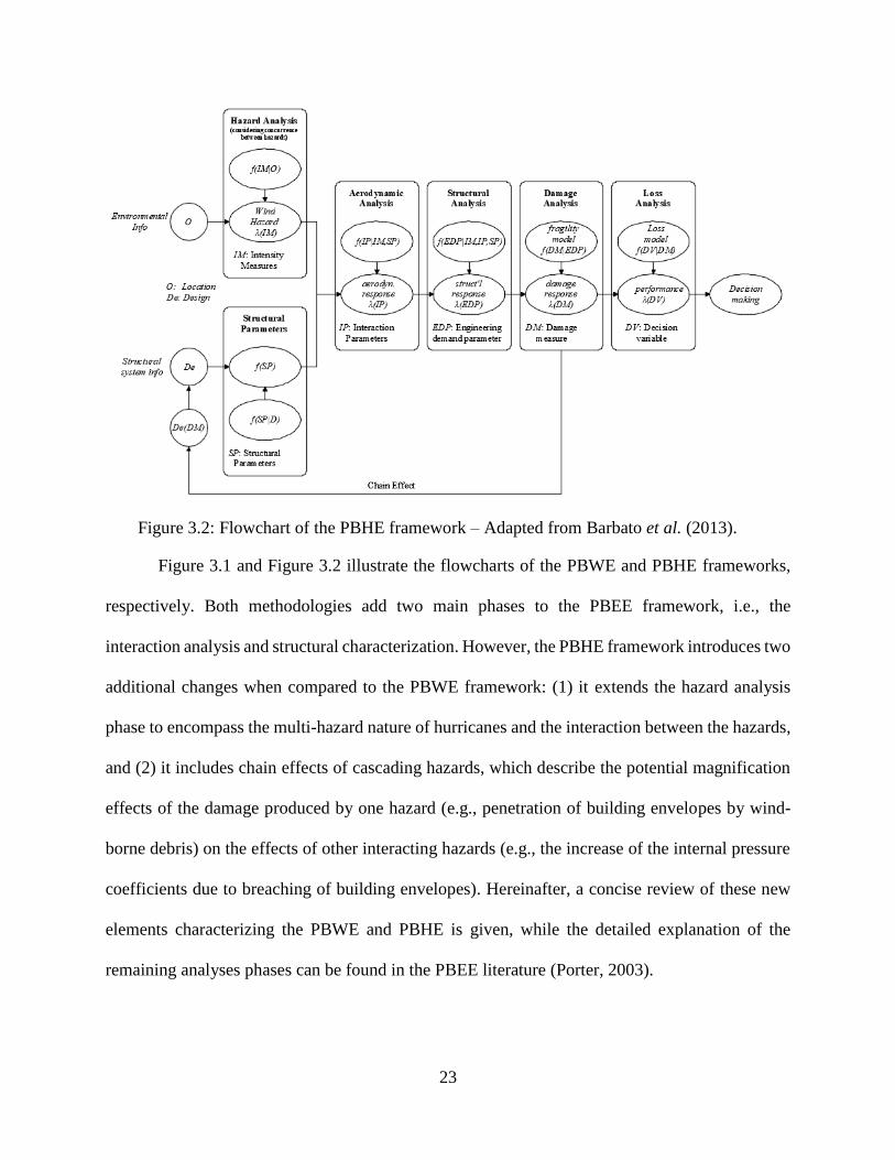
Figure 3.2: Flowchart of the PBHE framework – Adapted from Barbato et al. (2013).
Figure 3.1 and Figure 3.2 illustrate the flowcharts of the PBWE and PBHE frameworks,
respectively. Both methodologies add two main phases to the PBEE framework, i.e., the
interaction analysis and structural characterization. However, the PBHE framework introduces two
additional changes when compared to the PBWE framework: (1) it extends the hazard analysis
phase to encompass the multi-hazard nature of hurricanes and the interaction between the hazards,
and (2) it includes chain effects of cascading hazards, which describe the potential magnification
effects of the damage produced by one hazard (e.g., penetration of building envelopes by wind-
borne debris) on the effects of other interacting hazards (e.g., the increase of the internal pressure
coefficients due to breaching of building envelopes). Hereinafter, a concise review of these new
elements characterizing the PBWE and PBHE is given, while the detailed explanation of the
remaining analyses phases can be found in the PBEE literature (Porter, 2003).
24
3.1 Hazard analysis
In the PBWE framework, different IM vectors were adopted in the literature to describe the
wind hazard level, which depend mainly on the environmental information in terms of wind
exposure. In addition to the wind speed at 10m height above the ground (with different possible
averaging times), the wind direction and the roughness length z0 have been considered as IM
components as well (Petrini et al., 2010). Similarly to PBEE methodology, the IM vector must
satisfy the requirements of sufficiency and efficiency with respect to the EDP used in the analysis
(Luco and Cornell, 2007).
The PBHE extends the hazard analysis proposed for wind effects to include the effect of
the four main sources of hazard that are interacting during a hurricane event, i.e. (Barbato et al.,
2013):
(1) Gust winds producing the wind damage, described by a random vector W.
(2) Storm surge producing the flood damage, described by a random vector F.
(3) Windborne debris producing windborne debris impact damage, described by a random
vector D.
(4) Heavy rainfall producing high water levels, and damaging the interior of the structure
should the envelope be breached, described by a random vector R.
Furthermore, the independence or the interaction between the aforementioned hazard
sources is also included in the hazard analysis phase. Multiple hazards occurring individually or
simultaneously are independent if they hit the structure, but their actions can still be treated as
independent. By contrast, concurrently interacting hazards are the ones that hit the structure but
their actions are highly correlated (Petrini and Palmeri, 2012).
25
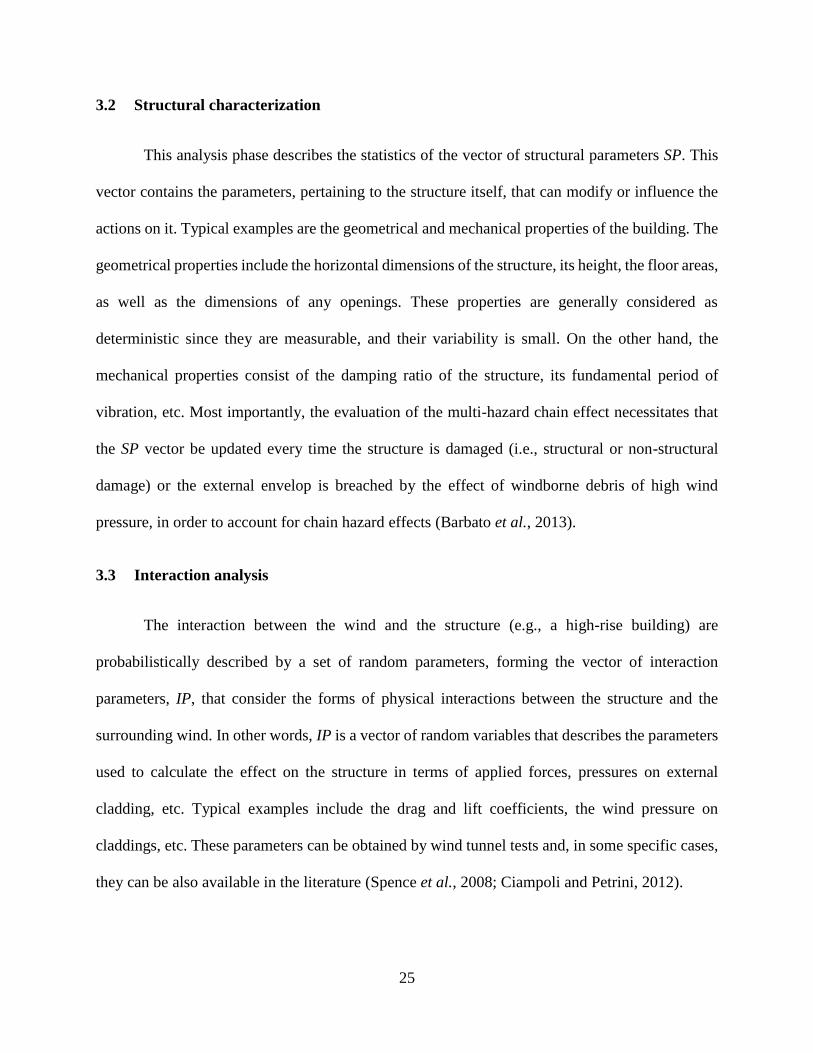
3.2 Structural characterization
This analysis phase describes the statistics of the vector of structural parameters SP. This
vector contains the parameters, pertaining to the structure itself, that can modify or influence the
actions on it. Typical examples are the geometrical and mechanical properties of the building. The
geometrical properties include the horizontal dimensions of the structure, its height, the floor areas,
as well as the dimensions of any openings. These properties are generally considered as
deterministic since they are measurable, and their variability is small. On the other hand, the
mechanical properties consist of the damping ratio of the structure, its fundamental period of
vibration, etc. Most importantly, the evaluation of the multi-hazard chain effect necessitates that
the SP vector be updated every time the structure is damaged (i.e., structural or non-structural
damage) or the external envelop is breached by the effect of windborne debris of high wind
pressure, in order to account for chain hazard effects (Barbato et al., 2013).
3.3 Interaction analysis
The interaction between the wind and the structure (e.g., a high-rise building) are
probabilistically described by a set of random parameters, forming the vector of interaction
parameters, IP, that consider the forms of physical interactions between the structure and the
surrounding wind. In other words, IP is a vector of random variables that describes the parameters
used to calculate the effect on the structure in terms of applied forces, pressures on external
cladding, etc. Typical examples include the drag and lift coefficients, the wind pressure on
claddings, etc. These parameters can be obtained by wind tunnel tests and, in some specific cases,
they can be also available in the literature (Spence et al., 2008; Ciampoli and Petrini, 2012).
26
4 APPLICATION EXAMPLE – PERFORMANCE-BASED HURRICANE
LOSS ASSESSMENT
4.1 Description of the structure and location
In order to illustrate the PBHE methodology to evaluate the expected annual losses, an
application example consisting of a high-rise building was considered. The structure is composed
of 74 stories, and the structural components (i.e., beams, columns, and braces) are made of steel
material characterized by a yield strength of 36 ksi (Steel A36). The typical story height is about
4.00 m, except for the first and roof floors whose heights are approximately 13.10 m and 4.75 m,
respectively.
The building (see Figure 4.1) has a symmetrical 51x51 m² (B = 51 m) floor plan and a total
height H = 305 m. Two substructures form the main structural system: a three-dimensional outer
frame formed by a total of 28 columns equally spaced on the external periphery and another three-
dimensional central core composed of 16 columns. Three stiffening truss systems connect the
internal and the external substructures at levels 24, 49, and 74. The columns have a square hollow
sections whose dimensions and thickness vary with respect to the height (1.20 m and 0.06 m floors
1-23, 0.9 m and 0.045 m for floors 24-48, and 0.5 m and 0.025 m for floors 49-74). The horizontal
beams are steel double-T sections rigidly connected to the columns at each side. The bracing
system consists of double-T section braces or hollow square struts. The building was considered
to be used for offices, and its total monetary value, including the contents (e.g., electrical and
mechanical equipment, computers), was assumed to be $329 million dollars. This building has
been extensively used in the literature, and further information about wind tunnel tests and details
of the model can be found in Ciampoli and Petrini (2012).
27
(a) (b) (c) (d) (e)
Figure 4.1: Finite Element model of the case study building: (a) 3D model; (b) external 3D
frame; (c) bracing system at 24-25th , 48-49th and 74th floors; (d) central core 3D fame;
and (e) plan view of the 74th floor.
The target structure was assumed to be located in Miami, FL, a major city on the south-
eastern coast of the United States, where hurricanes of various intensities occur almost every year.
Moreover, the city is prone to non-hurricane winds that should be also taken into account while
designing the structure. Their impact not only affects the ultimate limit state of design but also the
serviceability of the structure, which is represented mainly by the occupants’ comfort criteria that
should be met at any time. A failure to meet these criteria could render the structure unusable for
several days each year. In this case study, the only hurricane hazard source considered was the
hurricane wind. In fact, the building was assumed to be located sufficiently far from other buildings
(so that windborne debris and rainfall effects could be neglected) and from the coastline (so that
the storm surge effects could be neglected).
28
4.2 Details of the steps of the analysis
4.2.1 Hurricane wind hazard
Hurricanes are natural phenomena considered to be rare and extreme events, therefore their
recurrence rate can be modeled using a Poisson counting process characterized by an annual rate
of occurrence hurricane (Russell, 1971; Chouinard and Liu, 1997). Based on historical data
extracted from the Iowa Environmental Mesonet (IEM) database, measured at Miami International
Airport between the years 1962 and 2013, the annual rate is found to be equal to 0.54hurricane
(IEM, 2014). Similar results can be obtained from the National Institute of Standards and
Technology (NIST) database (NIST, 2017).
The IM vector used to describe the wind hazard has the following components:
(1) the 10-minute wind speed 10minV at 10 m above the ground level which was adopted to
calculate the structural response (i.e., peak displacements, PFA),
(2) the 3-second wind speed 3secV at 10 m above the ground level which was adopted to
calculate the local response (i.e., pressure on cladding),
(3) the wind directionality or angle of attack, and
(4) the site-specific roughness length 0z .
At each story level of the building, the wind speed ,u jV z t in the along-wind direction,
is the superposition of a zero-mean time-variant stochastic component ,u jv z t and a time-
independent non-zero mean value m jV z . The across and vertical wind speeds, ,v jV z t and
, ,w jV z t consist of time-dependent varying components, ,v jv z t and ,w jv z t respectively. All
29
three fluctuating components were considered to be independent ergodic zero-mean stationary
Gaussian random processes (Ciampoli and Petrini, 2012).
The wind velocities can be mathematically expressed as:
, ,
, ,
, ,
u j m j u j
v j v j
w j w j
V z t V z v z t
V z t v z t
V z t v z t
(4.1)
where jz is the vertical height of the j-th story above the ground, 1,2, , fj N ,
fN = total
number of stories of the target building, and t denotes time.
The along-wind mean velocity mV z , calculated in the atmospheric boundary layer over
a surface having a homogeneous roughness is a function of the height z and its expression is given
by the “power law” (Simiu and Scanlan, 1978):
m t e
zV z c c V z
z
(4.2)
where tc = conversion factor for different wind time averages,
ec = conversion factor for different
terrain exposure categories, z = 10 m, and is a site-dependent parameter given by (Holmes,
2014):
0
1
ln refz z (4.3)
where refz is taken equal to 50 m.
The historical data collected from the IEM database, which also contains other climatic
and weather-related archived records, consists of the 3-second wind gusts in terrain exposure D as
defined in the ASCE 7-10 (ASCE, 2010) measured at 10 m elevation above the ground for the
period 1962-2013. In addition, the hurricane tracks that passed within 250 miles radius around the
target location were gathered from the National Oceanic and Atmospheric Administration
30
(NOAA)’s database for the same period of time (Unnikrishnan, 2015). These tracks were used to
separate the hurricane wind speeds from the non-hurricane ones. The hurricane wind speeds were
fitted to a three-parameter Generalized Extreme Value type II distribution characterized by the
following CDF:
1
1
0;
; , ,
;
V
V
F V
e V
(4.4)
The statistical descriptors of this distribution, i.e., , , , which are site-specific parameters,
were obtained using the maximum likelihood estimation method and were found to be the
following: 32.4138, 6.2652, 0.6424 (Unnikrishnan, 2015). On the other hand, the
yearly maximum non-hurricane 10-minute wind speeds, evaluated by multiplying the maximum
yearly 3-second-averaged values by the time conversion coefficient ct=0.67 (Lungu and Rackwitz,
2001), were fitted to a lognormal distribution having a mean of 19.3 m/s and standard deviation of
0.5 m/s (Unnikrishnan, 2015). The structure was assumed to be located in an area characterized by
a terrain exposure category B as per the ASCE 7-10 standards (ASCE, 2010), therefore, the terrain
exposure conversion factor, ce, was found to be equal to 0.84 (Lungu and Rackwitz, 2001).
Furthermore, the randomness inherent to the wind directionality or the angle of attack θ
should be taken into account in the quantification of the wind hazard intensity. This variability
propagates through the wind-structure interaction parameters, namely the drag and lift coefficients,
to eventually alter the variability of the response and losses. For this purpose, the wind directions
were gathered from the historical data provided in the NOAA’s Solar and Meteorological Surface
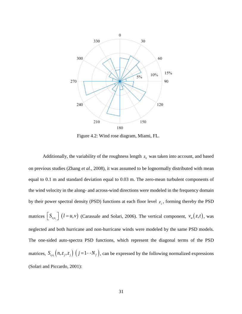
Observational Network (SAMSON) dataset over the years 1961-1990. The wind rose, depicted in
Figure 4.2, shows the percentage of time the wind blows from a certain direction in the target
location.
31
Figure 4.2: Wind rose diagram, Miami, FL.
Additionally, the variability of the roughness length 0z was taken into account, and based
on previous studies (Zhang et al., 2008), it was assumed to be lognormally distributed with mean
equal to 0.1 m and standard deviation equal to 0.03 m. The zero-mean turbulent components of
the wind velocity in the along- and across-wind directions were modeled in the frequency domain
by their power spectral density (PSD) functions at each floor level jz , forming thereby the PSD
matrices ,l lv vS l u v (Carassale and Solari, 2006). The vertical component, ,wv z t , was
neglected and both hurricane and non-hurricane winds were modeled by the same PSD models.
The one-sided auto-spectra PSD functions, which represent the diagonal terms of the PSD
matrices, , , 1l lv v j j fS n z z j N , can be expressed by the following normalized expressions
(Solari and Piccardo, 2001):
32
523
523
6.868, ,
1 10.302
9.434, ,
1 14.15
u u
u
v v
v
u j
m jv v j j
vu j
m j
v j
m jv v j j
vv j
m j
n L z
V zn S n z z
n L z
V z
n L z
V zn S n z z
n L z
V z
(4.5)
where jz is measured in meters, n is the frequency content of the wind measured in Hertz, and
the variances of the along- and across-wind velocities, 2
lv , are given by:
2 1 2 2
0 *6 1.1 tan ln 1.75 ,lv lz u l u v (4.6)
where *
0
ln
m
ku V z
z
z
is the shear velocity, 1.00, 0.75u v , k = 0.40 is the von
Karman’s constant, z = 10 m, l jL z are the integral length scales of the turbulent components
whose expressions are given by (Carassale and Solari, 2006):
00.67 0.05ln
300 ,200
z
j
l j l
zL z l u v
(4.7)
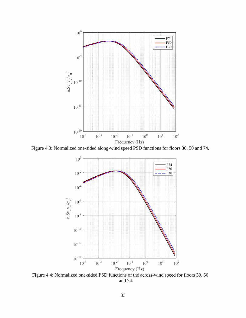
where 1.00, 0.25u v . Figure 4.3 and Figure 4.4 show the wind speed PSD functions in a
logarithmic scale at the 30th, 50th and 74th floors, in the along- and across-wind directions for a
mean 10-minute wind velocity at 10 m above the ground Vm = 35 m/s and a roughness length
0 0.1 m.z
33
Figure 4.3: Normalized one-sided along-wind speed PSD functions for floors 30, 50 and 74.
Figure 4.4: Normalized one-sided PSD functions of the across-wind speed for floors 30, 50
and 74.
34
The off-diagonal terms of the PSD matrices, , , , 1l lv v j k fS n z z j k N , which represent the
cross-spectra PSD functions between stories, are given by:
, , , , , , exp , , ,l l l l l lv v j k v v j j v v k k l j kS n z z S n z z S n z z f n z z l u v
(4.8)
in which , ,l j kf n z z is given by (Di Paola, 1998):
, , lz j k
l j k
m j m k
n C z zf n z z
V z V z
(4.9)
for vertically aligned points, where 10uzC and 6.5
vzC are the decay coefficients (Carassale
and Solari, 2006).
4.2.2 Structural characterization
In order to obtain the static and dynamic response of the building, a finite element model
was developed on STAAD.Pro (STAAD.Pro V8i, 2015). The dimensions of the structure were
assumed as deterministic and the diaphragms were considered rigid. The flexibility matrix was
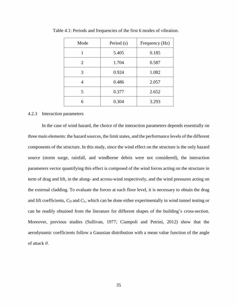
obtained along with the modal analysis results in terms of mode shapes and modal frequencies (see
Table 4.1). For this purpose, 6 modes of vibration corresponding to a total of 95% modal
participation mass ratio were considered, and the torsional effect was neglected. In the case study,
the damping ratios, q , of the different modes of vibration 1,2, ,6,q were assumed to be
statistically independent and following a lognormal distribution with a mean value of 0.02 and a
standard deviation of 0.008 (Ciampoli and Petrini, 2012). The model was assumed to be elastic at
all stages of the analysis. In other words, the structural parameters were assumed to remain intact
after the hurricane hit the structure and cause the damage.
35
Table 4.1: Periods and frequencies of the first 6 modes of vibration.
Mode Period (s) Frequency (Hz)
1 5.405 0.185
2 1.704 0.587
3 0.924 1.082
4 0.486 2.057
5 0.377 2.652
6 0.304 3.293
4.2.3 Interaction parameters
In the case of wind hazard, the choice of the interaction parameters depends essentially on
three main elements: the hazard sources, the limit states, and the performance levels of the different
components of the structure. In this study, since the wind effect on the structure is the only hazard
source (storm surge, rainfall, and windborne debris were not considered), the interaction
parameters vector quantifying this effect is composed of the wind forces acting on the structure in
term of drag and lift, in the along- and across-wind respectively, and the wind pressures acting on
the external cladding. To evaluate the forces at each floor level, it is necessary to obtain the drag
and lift coefficients, CD and CL, which can be done either experimentally in wind tunnel testing or
can be readily obtained from the literature for different shapes of the building’s cross-section.
Moreover, previous studies (Sullivan, 1977; Ciampoli and Petrini, 2012) show that the
aerodynamic coefficients follow a Gaussian distribution with a mean value function of the angle
of attack θ.
36
The coefficient of variation (COV) of the drag coefficient was taken equal to 5%, whereas
the standard deviation1 of the lift coefficient was taken equal to 0.038.
The PSD matrices, ,l lF FS l u v , of the forces applied at each floor of the building can
be obtained based on the IPs and the PSD functions of the wind velocity. The general term of the
along-wind force matrix is given by:
, , , , , ,u u u uF F j k j j v v j k k kS n z z A z n z S n z z n z A z (4.10)
where , 1,2, , fj k N ,
j air D j m jA z C Ar z V z (4.11)
in which air is the mass density of the air, jAr z is the exposed wind tributary area of the j-th
floor, , jn z is the aerodynamic admittance function given by (Holmes, 2014):
43
1,
21
j
j
m j
n z
n Ar z
V z
(4.12)
On the other hand, the general term of the across-wind force matrix is given by:
2
2
, ,1 1, ,
2
v v
v v
v
v v j k
F F j k air L m j m k j k
v
n S n z zS n z z C V z V z Ar z Ar z
n
(4.13)
In general, the across-wind force is the superposition of:
(1) the turbulent effect, and
(2) the vortex shedding2 or vortex-induced vibrations’ effect.
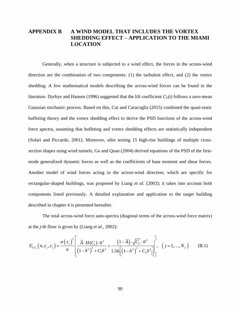
1 Refer to APPENDIX A for calculation of the standard deviation of the lift coefficient. 2 Refer to APPENDIX B for the results of the analysis obtained by using a model of across-wind
forces taking into account the vortex shedding effect.
37
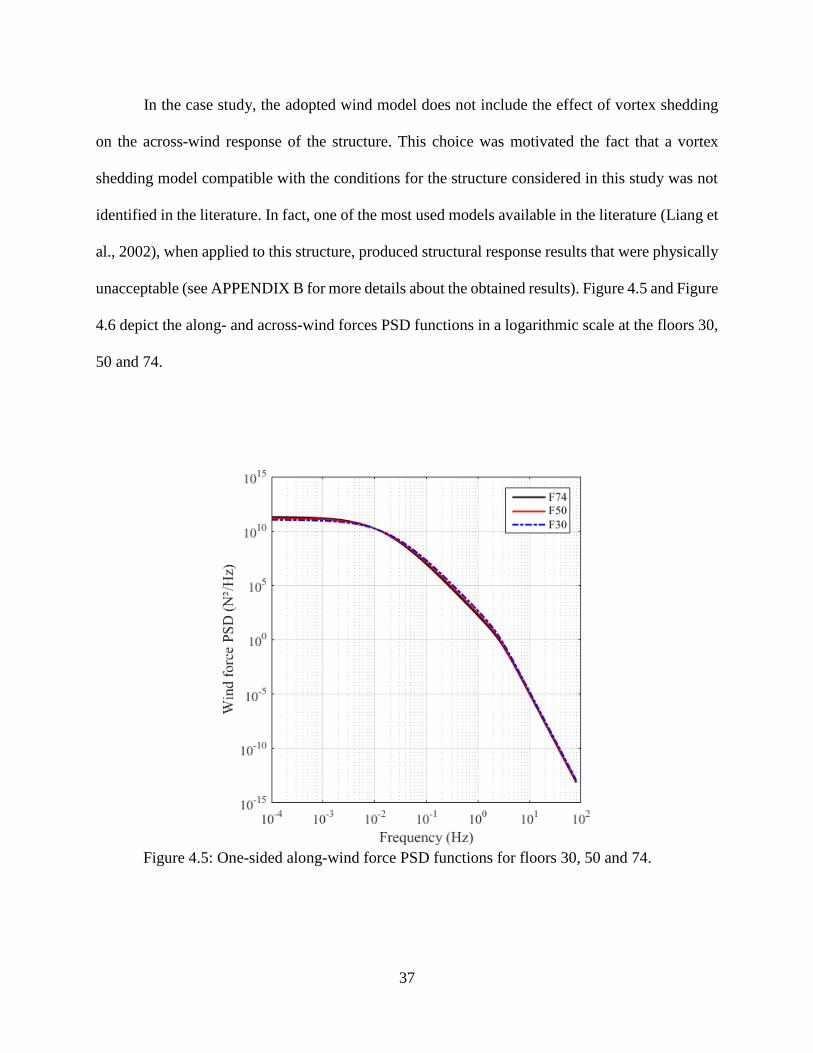
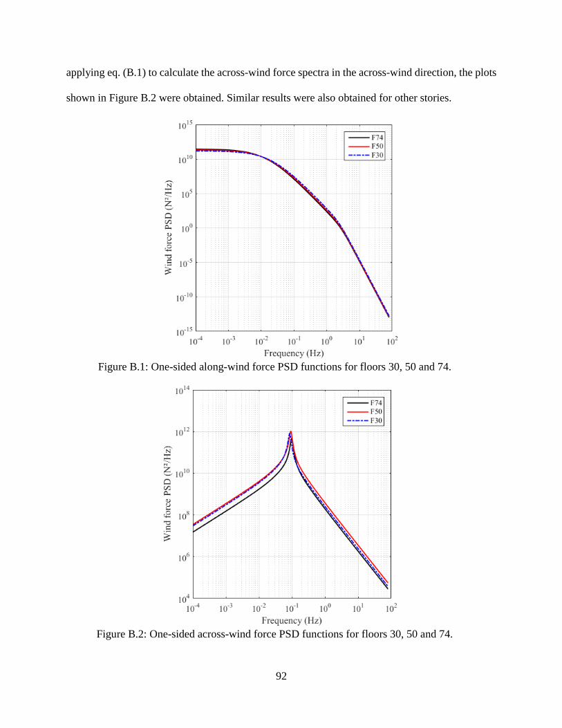
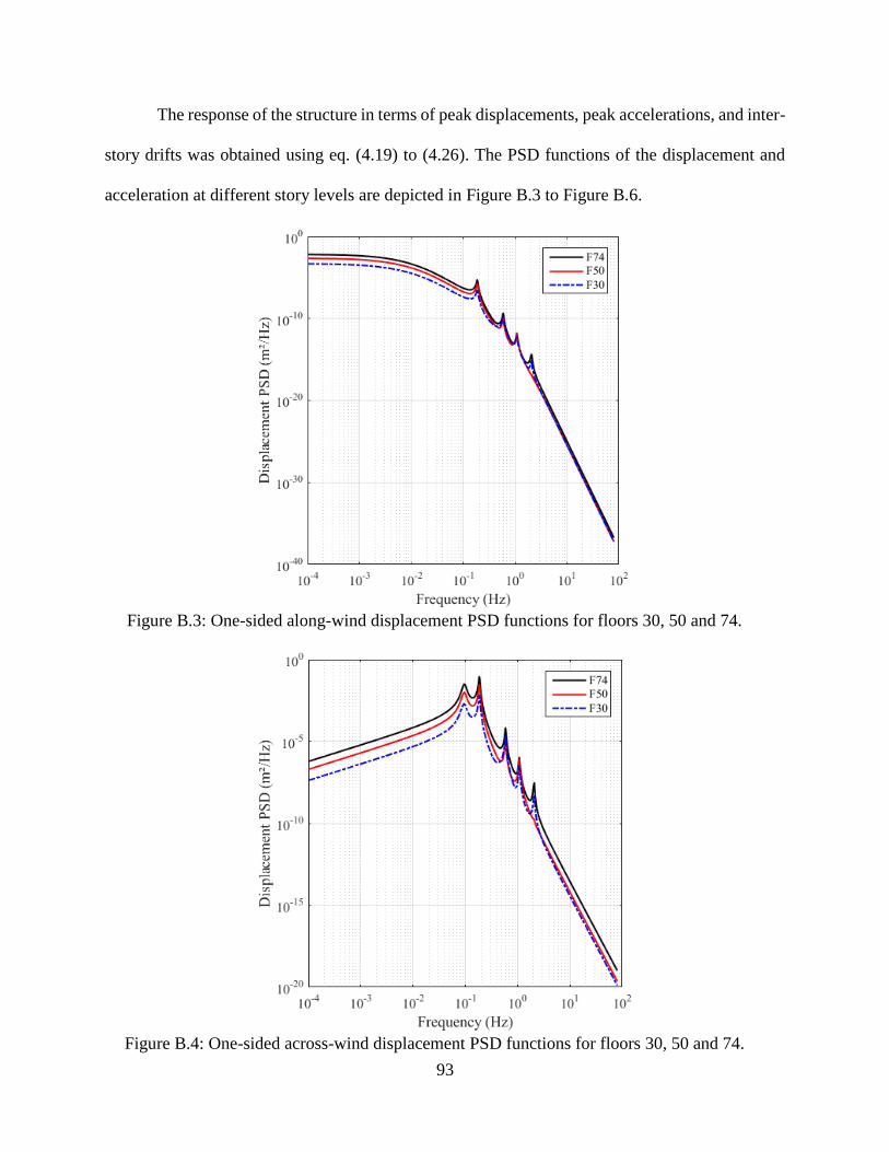
In the case study, the adopted wind model does not include the effect of vortex shedding
on the across-wind response of the structure. This choice was motivated the fact that a vortex
shedding model compatible with the conditions for the structure considered in this study was not
identified in the literature. In fact, one of the most used models available in the literature (Liang et
al., 2002), when applied to this structure, produced structural response results that were physically
unacceptable (see APPENDIX B for more details about the obtained results). Figure 4.5 and Figure
4.6 depict the along- and across-wind forces PSD functions in a logarithmic scale at the floors 30,
50 and 74.
Figure 4.5: One-sided along-wind force PSD functions for floors 30, 50 and 74.
38
Figure 4.6: One-sided across-wind force PSD functions for floors 30, 50 and 74.
Another component of the IP vector is the wind pressure, w jp z , acting on the external
cladding of the building at each floor height. As formulated in the ASCE 7-10 (ASCE, 2010)
standards, the wind pressure on the cladding at the j-th floor is given by:
w j j p pip z q z GC GC (4.14)
where
20.613 SI unitsj zt m jq z K V z (4.15)
in which ztK is the topographic factor assumed to be deterministically equal to 1.
4.2.4 Structural analysis
The peak values of the response in terms of displacements and accelerations were obtained
by performing the structural analysis in the frequency domain (Clough and Penzien, 1993). This
approach is easier than performing the analysis in the time domain because the model was
39
considered to be linear elastic and the applied forces were given in terms of PSD functions. The
inter-story drift in the along- and across-wind directions at the j-th floor are expressed as the
difference of displacements between the j-th and the (j-1)-th floors, i.e.,
1
1
u j u j u j
v j v j v j
I z D z D z
I z D z D z
(4.16)
where u jD z and v jD z are the along- and across-wind displacements at story j; the PFA in
the along- and across-wind directions are denoted u jA z and v jA z respectively.
Based on random vibration theory results, the response of the structure in terms of PSD
matrices of the displacements and the accelerations can be obtained by applying the following
equations (Carassale et al., 2001):
* T T
1 1
4 * T T
1 1
( ) ( ) ( ) , ( , )
2 ( ) ( ) ( ) ,( , )
l l l l
l l l l
N N
D D q p q q F F p p
p q
N N
A A q p q q F F p p
p q
S n H n H n S n l u v
S n n H n H n S n l u v
(4.17)
where N’ is the number of modes, q is the mass-normalized mode shape vector of the q-th mode,
( )qH n is the frequency response function for the corresponding mode of vibration and can be
calculated by:
2 2 2
1 1( )
4 2q
q q q q
H nM n n i n n
(4.18)
where qn and qM are the natural frequency and modal mass of the q-th mode of vibration,
respectively, 1,i the superscript T is the transpose operator, and the superscript * indicates
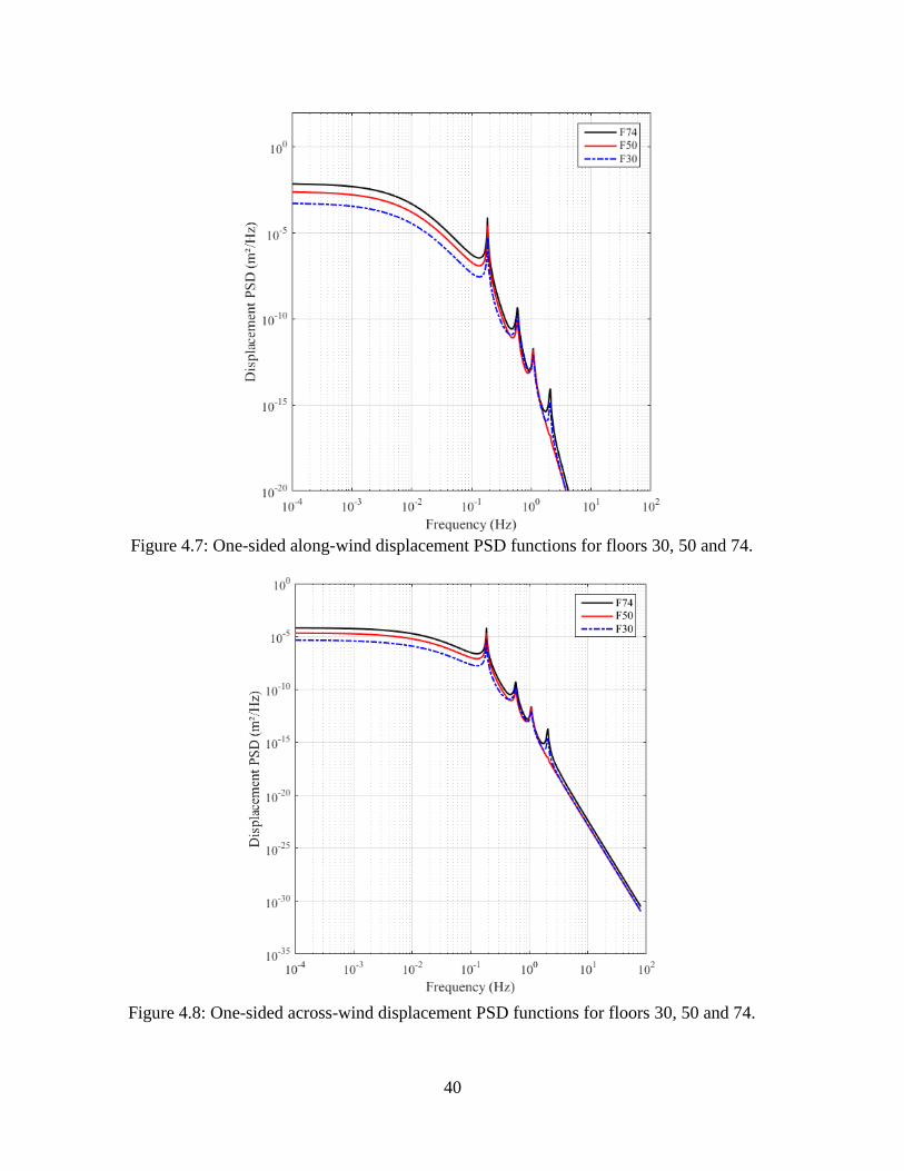
the complex conjugate value of the function. Figure 4.7 to Figure 4.10 show the displacement and
acceleration auto-PSD functions at floor 30, 50, and 74, in the along- and across-wind directions.
40
Figure 4.7: One-sided along-wind displacement PSD functions for floors 30, 50 and 74.
Figure 4.8: One-sided across-wind displacement PSD functions for floors 30, 50 and 74.
41
Figure 4.9: One-sided along-wind acceleration PSD functions for floors 30, 50 and 74.
Figure 4.10: One-sided across-wind acceleration PSD functions for floors 30, 50 and 74.
42
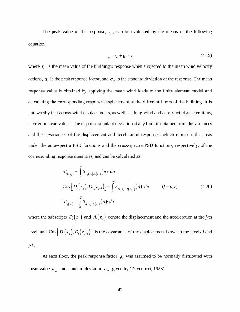
The peak value of the response, pr , can be evaluated by the means of the following
equation:
p m r rr r g (4.19)
where mr is the mean value of the building’s response when subjected to the mean wind velocity
actions, rg is the peak response factor, and r is the standard deviation of the response. The mean
response value is obtained by applying the mean wind loads to the finite element model and
calculating the corresponding response displacement at the different floors of the building. It is
noteworthy that across-wind displacements, as well as along-wind and across-wind accelerations,
have zero mean values. The response standard deviation at any floor is obtained from the variances
and the covariances of the displacement and acceleration responses, which represent the areas
under the auto-spectra PSD functions and the cross-spectra PSD functions, respectively, of the
corresponding response quantities, and can be calculated as:
1
2
0
1
0
2
0
Cov , ( , )
l j l j l j
l j l j
l j l j l j
D z D z D z
l j l j D z D z
A z A z A z
S n dn
D z D z S n dn l u v
S n dn
(4.20)
where the subscripts l jD z and l jA z denote the displacement and the acceleration at the j-th
level, and 1Cov ,l j l jD z D z is the covariance of the displacement between the levels j and
j-1.
At each floor, the peak response factor rg was assumed to be normally distributed with
mean value rg and standard deviation
rg given by (Davenport, 1983):
43
wind
wind
wind
0.5772ln
2ln
π
12ln
r
r
g
g
TT
T
(4.21)
where is the effective frequency of the structure which is conservatively taken as 1n , the
fundamental natural frequency of the structure, and windT is the interval of time where the peak
response is calculated.
Applying eq. (4.19) to the demand parameters, the peak responses are evaluated as follows:
(1) the peak displacement in the along-wind direction at floor j, ,u p jD z , is given by:
, ,u u ju p j m j D j D z
D z D z g (4.22)
(2) the peak displacement in the across-wind direction at floor j, ,v p jD z , is given by:
, ,v v jv p j D j D z
D z g (4.23)
(3) the inter-story drift in the along-wind direction at floor j, ,pu jI z , is given by:
1
2 2
, 1 , 12 Cov ,u u j u j
u p j m j m j I j u j u jD z D zI z D z D z g D z D z
(4.24)
(4) the inter-story drift in the across-wind direction at floor j, ,v p jD z , is given by:
1
2 2
,p , 12 Cov ,v v j v j
v j I j v j v jD z D zI z g D z D z
(4.25)
(5) the PFA in the along- and across-wind direction at floor j, ,l p jA z , is given by:
, , ,l l j
l p j A j A zA z g l u v (4.26)
where,
m jD z is the mean along-wind displacement at the j-th floor,
u jD z is the standard deviation of the along-wind displacement at the j-th floor,
44
,uD jg is the peak factor for the j-th along-wind displacement,
v jD z is the standard deviation of the across-wind displacement at the j-th floor,
,vD jg is the peak factor for the j-th across-wind displacement,
1Cov ,u j u jD z D z
is the covariance of the along-wind displacements at the j-th and the
(j-1)-th floors,
,uI jg is the peak factor for the j-th along-wind inter-story drift,
1Cov ,v j v jD z D z
is the covariance of the across-wind displacements at the j-th and the
(j-1)-th floors,
,vI jg is the peak factor for the j-th across-wind inter-story drift,
l jA z is the standard deviation of the acceleration response in the l-th direction, and
,lA jg is the peak factor for the j-th acceleration response in the l-th direction.
4.2.5 Damage analysis
The estimation of the losses was performed using the story-based approach (Ramirez and
Miranda, 2009). Accordingly, the damage states and the fragility curves are functions of the
different component groups. For this purpose, the parameters of the fragility curves of each
component group, given by eq. (2.16), were obtained from HAZUS (FEMA, 2015a), and they are
summarized in Table 4.2.
45
Table 4.2: Fragility curve parameters for different component groups.
Component group
Slight
damage
Moderate
damage
Extensive
damage
Complete
damage
EDP DS EDP DS
EDP DS
EDP DS
EDP DS EDP DS
EDP DS
EDP DS
Structural drift-sensitive
components
(Inter-story drift ratio)
0.25% 0.40 0.50% 0.40 1.50% 0.40 4.00% 0.40
Non-structural drift-
sensitive components
(Inter-story drift ratio)
0.40% 0.50 0.80% 0.50 2.50% 0.50 5.00% 0.50
Non-structural
acceleration-sensitive
components (Floor
acceleration, (g))
0.30 0.60 0.60 0.60 1.20 0.60 2.40 0.60
Figure 4.11, Figure 4.12, and Figure 4.13 show the fragility curves for the different
component groups (i.e., structural drift-sensitive, non-structural drift-sensitive, non-structural
acceleration-sensitive).
46
Figure 4.11: Fragility curves of the structural drift-sensitive component group.
Figure 4.12: Fragility curves of the non-structural drift-sensitive component group.
47
Figure 4.13: Fragility curves of the non-structural acceleration-sensitive component group.
For a given value of the demand parameter, i.e., MIDR or PFA at story j, the probability that
a group of components reaches each of the damage states was calculated, then a randomly selected
damage state weighted with the corresponding probability was assigned to that group of
components.
4.2.6 Loss analysis
The loss estimation was performed using the multilayer MCS approach. For an accurate
estimation of the expected annual losses and a correct evaluation of the annual rate of exceedance
of a repair cost, which was used as the DV, 10,000 random samples were generated and used to
obtain the results (see Figure 4.14).
48
Figure 4.14: Convergence of the losses using the multilayer MCS technique.
The repair costs for each damage state for each group of components were considered to
be lognormally distributed and were generated based on the mean values given in Table 4.3 and a
COV equal to 10% (FEMA, 2015a). In addition, the serviceability limit state in terms of occupants’
discomfort was also taken into account. The human tolerance threshold of the wind-induced
vibrations in high-rise structures was considered to be deterministic and expressed in terms of
acceleration values. For the target structure, which was assumed to be an office building, the
acceleration threshold above which the occupants start to feel uncomfortable was taken as 0.15
m/s² (Ciampoli and Petrini, 2012). HAZUS (FEMA, 2015a) described the losses incurred by the
structure each day of business interruption due to an exceedance of the human perception
acceleration threshold as lognormally distributed with a mean value of $0.95 per square foot of
any given floor and a COV of 10%. During a hurricane, which duration was considered to be
uniformly distributed between 1 and 3 days, the whole building was assumed to be closed if the
human perception threshold was exceeded in at least half of the total number of floors of the
building, otherwise, only the floors at which the acceleration threshold was exceeded were
considered closed. On the other hand, to evaluate the losses due to discomfort during non-hurricane
winds, the yearly maximum wind speed was checked if it caused any upcrossing of the perception
49
threshold during a one-year simulation. In case this threshold was upcrossed, the minimum yearly
wind speed causing exactly the perception threshold (i.e., an acceleration equal to 0.15 m/s²) was
calculated by scaling down the annual maximum wind speed by assuming that it can be represented
by a linear function of the PFA. Then, daily maximum wind velocities for a number of days equal
to 364 minus the duration, in days, of all the hurricane events that occurred that year was randomly
generated using a lognormal distribution capped on the upper tail to the annual maximum wind
speeds. The mean value of this lognormal distribution was obtained by taking into account the
high correlation between the mean daily maximum wind velocity over a one-year period and the
yearly maximum wind speed. The standard deviation of the distribution was calculated based on
the entire historical data of daily maximum wind speeds, because the standard deviation of the
daily maximum wind speeds was found to be approximately constant over the different years. The
number of days for which the daily maximum wind speed exceeded the minimum velocity
threshold was used to calculate the annual losses due to the business interruption. Similarly to
hurricane winds, the entire building was assumed to be closed for one day if the daily acceleration
was exceeded in at least half of the number of floors of the building; otherwise, only the floors at
which the acceleration threshold was exceeded were considered closed.
Table 4.3: Mean repair costs for the component groups at each damage state (in % of floor
cost).
Component group Slight
damage
Moderate
damage
Extensive
damage
Complete
damage
Drift-sensitive, structural
components 0.4 1.9 9.6 19.2
Drift-sensitive, non-
structural components 0.7 3.3 16.4 32.9
Acceleration-sensitive,
non-structural components 0.9 4.8 14.4 47.9
50
Furthermore, the pressure-sensitive components consist of the external façade of the
building, which was assumed to be entirely formed of 3.5x6.5 sqft ¼in-thick glass panels. The
failure of the window panel occurred when the applied wind-induced pressure, calculated using
eq. (4.14), exceeded the pressure resistance of the panel. It is noteworthy that the effects of
windborne debris impact due to high-speed hurricane winds were not included in this analysis.
Wind pressures at the 74 different levels exerted on each side of the building (i.e., windward,
leeward, and side facades) were compared to the resistance of the windows assumed to be normally
distributed with mean equal to 2500 N/m² (52.2 psf) and a COV of 20% (Gurley et al., 2005). The
statistical descriptors of the pressure coefficients as well as their distribution types were obtained
from the literature (Li and Ellingwood, 2006; Unnikrishnan and Barbato, 2017). The mean value
of the replacement cost of the exterior windows expressed in percentage of the total floor cost was
obtained from the literature and found to be 5.4% with a COV equal to 20% (Ramirez and Miranda,
2009).
4.2.7 Loss analysis results
Figure 4.15 and Figure 4.16 depict the annual probability of exceedance of the peak
displacement and the peak acceleration at the 74th floor in both the along-wind and across-wind
directions in a semi-logarithmic scale. From the obtained results, it can be noted that the annual
probability of exceedance for the displacement response in the along-wind direction is higher than
the one in the across-wind direction. This result is mainly due to the fact that the displacement in
the along-wind direction is the sum of a mean value of displacement produced by the time-
independent mean wind velocity component and a fluctuating time-variant component, whereas
the across-wind displacement depends only on the fluctuating time-variant component.
51
Figure 4.15: Annual probability of exceedance of the peak displacement response at the 74th
floor.
Figure 4.16: Annual probability of exceedance of the peak acceleration response at the 74th
floor.
52
On the other hand, the annual probability of exceeding the peak acceleration in the across-wind
direction is higher than the one in the along-wind due to the high turbulence intensity created in
the across-wind direction.
The annual probabilities of loss exceedance for the building, evaluated for different limit
states and plotted in semi-logarithmic scale, are depicted in Figure 4.17 together with the total
losses incurred by the structure for both hurricane winds (Hw) and non-hurricane winds (NHw).
The expected annual losses (EALs) along with the standard deviations of losses (SDL), as well as
the EALs conditional on losses greater than zero (EAL | Lossi > 0) with the standard deviation of
losses conditional on losses greater than zero (SDL | Lossi > 0) are listed in Table 4.4.
Figure 4.17: Annual probability of loss exceedance incurred by the target building due to
hurricane wind hazard.
53
Table 4.4: Expected annual losses and the corresponding standard deviation in thousand USD.
Losses
EAL
(in thousand
USD)
SDL
(in thousand
USD)
EAL | Lossi1 >0
(in thousand
USD)
SDL | Lossi > 0
(in thousand
USD)
Structural NHw < 1.00 3.50 18.26 5.02
Structural Hw 165.00 1,018.00 1,285.60 2,576.80
Non-structural NHw < 1.00 3.16 31.68 6.90
Non-structural Hw 140.00 947.00 1,473.80 2,740.70
Serviceability NHw < 1.00 < 1.00 < 1.00 < 1.00
Serviceability Hw 41.00 407.00 2,060.90 2,044.30
Cladding NHw 61.00 297.00 479.87 699.23
Cladding Hw 418.00 1,189.00 2,457.70 1,813.50
Total 827.00 3,073.00 2,629.40 5,030.60
1 The subscript i indicates the losses correspondent to the i-th damage state.
In an attempt to compare the effect of the variability of the angle of attack on the total
annual losses the building could expect, two different analyses were performed each with a
different angle of attack, i.e., 0 and 45 degrees respectively, then compared with the previous
results obtained with the actual wind directions weighted with the probabilities depicted in the
wind rose (Figure 4.2). An angle of attack equal to 0 degree corresponds to a wind blowing
perpendicularly to the upwind façade of the building, whereas a 45 degrees angle of attack
corresponds to a wind direction collinear with the building horizontal cross-section diagonal line
(diamond-shaped building).
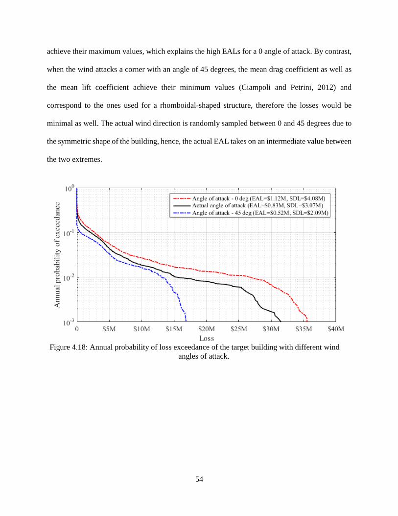
Figure 4.18 shows the annual probabilities of loss exceedance in a semi-logarithmic scale
for different wind directions along with the corresponding EALs and SDLs. It is observed that
when the wind is perpendicular to the upwind façade of the building, the expected annual losses
are the highest while the losses are minimal when the wind blows on the corner of the structure.
On the other hand, the actual EALs are somewhere in between these two extremes values. The
mean value of the drag coefficient is at its maximum when the wind is perpendicular to the upwind
façade (Ciampoli and Petrini, 2012) and consequently, the forces applied to the structure also
54
achieve their maximum values, which explains the high EALs for a 0 angle of attack. By contrast,
when the wind attacks a corner with an angle of 45 degrees, the mean drag coefficient as well as
the mean lift coefficient achieve their minimum values (Ciampoli and Petrini, 2012) and
correspond to the ones used for a rhomboidal-shaped structure, therefore the losses would be
minimal as well. The actual wind direction is randomly sampled between 0 and 45 degrees due to
the symmetric shape of the building, hence, the actual EAL takes on an intermediate value between
the two extremes.
Figure 4.18: Annual probability of loss exceedance of the target building with different wind
angles of attack.
55
5 APPLICATION EXAMPLE – PERFORMANCE-BASED MULTI-
HAZARD LOSS ASSESSMENT
The location where a structure is erected can be prone to multiple natural hazards that are
very different in nature, such as earthquake and wind. In order to perform a proper assessment of
the losses incurred by buildings in such locations, it is compulsory to quantify the expected damage
resulting from each of these hazards and evaluate the structural performance under different
hazards in a consistent manner. For this purpose, the same high-rise building utilized in the
previous chapter to evaluate the losses due to hurricane events is assumed to be located in one of
the regions where earthquake and wind hazards are both present. The chosen location is New
Madrid, Missouri. This location is characterized by a high seismicity level, as it is reflected on the
national seismic hazard maps. In particular, the USGS and the Center for Earthquake Research
and Information of the University of Memphis estimated the probability of occurrence of an
earthquake similar to the events that took place in the region in 1811-1812 (i.e., with a magnitude
between 7.5 and 8.0 on the Richter scale) is around 10% in 50 years, whereas the likelihood of
having a Richter magnitude greater than 6.0 during the same period of time is between 25% and
40% (Gomberg and Schweig, 2007). Moreover, this region is also subjected to wind exposures
(FEMA DR-1699-RA1, 2007), which necessitates that any design of high-rise structures must take
into account the corresponding wind-induced effects. The detailed description of the target
building can be found in chapter 4 of this thesis, and the following sections explain the different
steps of the analysis pursued to obtain an appropriate loss estimation of the different damaged
components due to the effect of earthquake and wind.
56
5.1 Seismic loss assessment
For the evaluation of the losses due to seismic loadings, two methods were investigated:
The first one was the analytical closed-form solution proposed by Jalayer and Cornell (2003), and
the second one was the multilayer MCS technique (Conte and Zhang, 2007). Both approaches are
explained in detail in the following sections.
5.1.1 Analytical closed-form solution
5.1.1.1 Hazard levels
The seismic hazard curve (i.e., the MAR of exceedance a given value of IM) for the
specified location was obtained by using the Unified Hazard Tool from the USGS website (USGS,
2017c) (Figure 5.1). In the current study, the 5%-damped spectral acceleration at the fundamental
period of the structure, 1, 5%aS T , was used as the seismic hazard IM. The target building’s
first mode of vibration is characterized by a period approximately equal to 5.4 s (Table 4.1). The
modal analysis was performed using STAAD.Pro (STAAD.Pro V8i, 2015), and the maximum
number of modes was chosen equal to six, so that the modal participating mass ratio was at least
equal to 95 % of the total mass of the building. Figure 5.1 shows the hazard curve obtained from
the USGS website for a period of vibration corresponding to the fundamental period of the target
structure.
57
Figure 5.1: Seismic hazard analysis (SHA) curve for spectral acceleration, New Madrid, MO.
As shown in Figure 5.1, the regression line approximation of the hazard curve in a
logarithmic scale consistently with eq. (2.4) was calculated as:
1
0.728
( ) ( ) 0.0002aS T a as s (5.1)
where, 1( ) ( )
aS T as is the MAR of the 5%-damped spectral acceleration at the fundamental period
of vibration exceeds sa, 0 0.0002k and 0.728k .
5.1.1.2 Structural response
The main purpose of this phase of the analysis is to obtain a statistical sample of the
response (i.e., EDP) of the structure at each floor, in terms of MIDR and absolute PFA, for each
level of ground motion intensity. Then, assuming that the response of the structure for any given
IM level can be described by a lognormally distributed random variable, the median EDPs were
calculated then fitted to a regression curve in the logarithmic scale to obtain an equation similar to
eq. (2.12).
In the current study, the structure was assumed to be linear elastic at all time; albeit
crucially important in general, nonlinear behavior was not considered in this application example
58
because it was expected that nonlinear behavior (corresponding to structural damage) is reached
only rarely under very intense seismic excitations, thus affecting only in a minor way the estimates
of the losses. A set of fifteen earthquake ground motion records were chosen from the PEER center
database (PEER, 2017a) to perform the linear time-history analysis (see Table 5.1). These records
were chosen so that they reflect the same properties of the source-site-structure combination for
this application example, so that the EDPs can be effectively estimated (Shome and Cornell, 1999).
The properties considered here were the type of source faults that are ruptured, the time-averaged
shear-wave velocity to 30 m depth (Vs30), the minimum and maximum magnitudes, and the fault
directivity effect. The properties of the site were found on the USGS website (USGS, 2017a,
2017b) and are: strike-slip fault type, Vs30 range is between 180 m/s and 240 m/s, the minimum
and maximum magnitudes are 6.5 and 8.0 respectively, and no directionality effect was considered.
Table 5.1: Earthquake recordings used in the structural analysis
Earthquake name Record number Year Station name
Imperial Valley-02 Rec. 1 1940 El Centro Array #9
Northwest Calif-02 Rec. 2 1941 Ferndale City Hall
Borrego Rec. 3 1942 El Centro Array #9
Northern Calif-03 Rec. 4 1954 Ferndale City Hall
El Alamo Rec. 5 1956 El Centro Array #9
Borrego Mtn Rec. 6 1968 El Centro Array #9
Borrego Mtn Rec. 7 1968 LB - Terminal Island
San Fernando Rec. 8 1971 Carbon Canyon Dam
San Fernando Rec. 9 1971 Cholame - Shandon Array #2
San Fernando Rec. 10 1971 LB - Terminal Island
Imperial Valley-06 Rec. 11 1979 Bonds Corner
Imperial Valley-06 Rec. 12 1979 Calexico Fire Station
Imperial Valley-06 Rec. 13 1979 Calipatria Fire Station
Imperial Valley-06 Rec. 14 1979 El Centro Array #1
Imperial Valley-06 Rec. 15 1979 El Centro Array #11
59
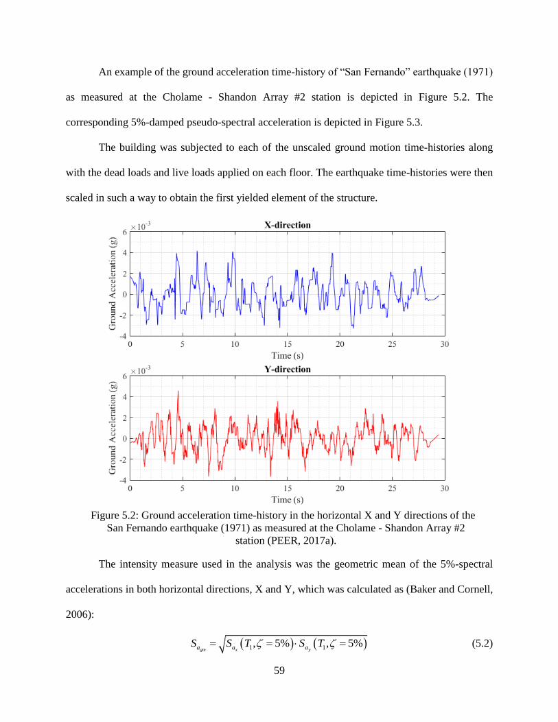
An example of the ground acceleration time-history of “San Fernando” earthquake (1971)
as measured at the Cholame - Shandon Array #2 station is depicted in Figure 5.2. The
corresponding 5%-damped pseudo-spectral acceleration is depicted in Figure 5.3.
The building was subjected to each of the unscaled ground motion time-histories along
with the dead loads and live loads applied on each floor. The earthquake time-histories were then
scaled in such a way to obtain the first yielded element of the structure.
Figure 5.2: Ground acceleration time-history in the horizontal X and Y directions of the
San Fernando earthquake (1971) as measured at the Cholame - Shandon Array #2
station (PEER, 2017a).
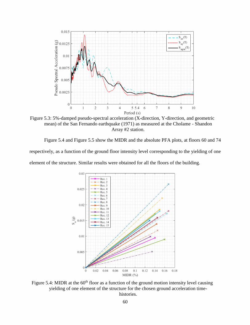
The intensity measure used in the analysis was the geometric mean of the 5%-spectral
accelerations in both horizontal directions, X and Y, which was calculated as (Baker and Cornell,
2006):
1 1, 5% , 5%gm x ya a aS S T S T (5.2)
60
Figure 5.3: 5%-damped pseudo-spectral acceleration (X-direction, Y-direction, and geometric
mean) of the San Fernando earthquake (1971) as measured at the Cholame - Shandon
Array #2 station.
Figure 5.4 and Figure 5.5 show the MIDR and the absolute PFA plots, at floors 60 and 74
respectively, as a function of the ground floor intensity level corresponding to the yielding of one
element of the structure. Similar results were obtained for all the floors of the building.
Figure 5.4: MIDR at the 60th floor as a function of the ground motion intensity level causing
yielding of one element of the structure for the chosen ground acceleration time-
histories.
61
Figure 5.5: PFA at the 74th floor as a function of the ground motion intensity level causing
yielding of one element of the structure for the chosen ground acceleration time-
histories.
Figure 5.6 plots the MIDR and PFA of the structure when the building is subjected to the
San Fernando earthquake time-history as measured at the Cholame - Shandon Array #2 station
when the first element of the structure was plasticized. Similar results were obtained for the other
14 ground motion time-histories.
62
(a) (b)
Figure 5.6: Structural response: (a) maximum inter-story drift ratio, and (b) peak floor
acceleration response profiles for San Fernando earthquake (1971) as measured at the
Cholame - Shandon Array #2 station.
Since the model was assumed to be linear elastic, the curves shown in Figure 5.4 and Figure
5.5 can be extended linearly to reach the intensity levels corresponding to probabilities of seismic
ground motion exceedance equal to 50% in 30 years, 10% in 50 years, and 2% in 50 years
respectively. The ground acceleration values, relative to each of the aforementioned levels, were
obtained from the hazard curve (see Figure 5.1), or calculated using the linear regression line in
the logarithmic scale using eq. (5.1). This approach is accurate only in the case of events derived
from a Poisson process having very small probabilities of occurrence, for which the mean annual
rate and the probability of exceedance (or probability of failure) are approximately the same
(Jalayer and Cornell, 2003), which correspond to the conditions for the present application
example. Then, at each floor level, the median values of the EDP, conditional to the level of
1, 5%aS T , were fitted to a regression curve in the logarithmic scale similar to eq. (2.12).
63
Moreover, the standard deviation EDP IM , of the natural logarithm of the response, conditional on
a ground motion intensity level, was calculated. Since the model is linear elastic, this standard
deviation is a constant value for any seismic intensity level.
5.1.1.3 Damage and loss assessment
The story-based damage evaluation was adopted in this study (Ramirez and Miranda, 2009;
Unnikrishnan and Barbato, 2017). In order to quantify the MAR of exceeding a damage state, the
median values of the EDP corresponding the each of the damage states were collected from
HAZUS (FEMA, 2015a); they are summarized in Table 4.2. Four damage states were considered:
(1) slight damage, (2) moderate damage, (3) extensive damage, and (4) complete damage. The
MAR of exceeding a certain damage state i, i.e., iDS , i=1, 2, 3, 4, was then calculated using the
closed-form equation given by eq. (2.17) (Jalayer and Cornell, 2003). These calculations were
repeated for all the stories of the building.
Furthermore, using the fact that the damage states are discrete, the MAR of exceeding a
repair cost, which was used as the decision variable DV in the analysis, was calculated by applying
eq. (2.19) for each floor level. The losses were assumed to be lognormally distributed with
statistical descriptors listed in Table 4.3. Therefore, the probability of exceeding a certain dv value,
i.e., repair cost in USD, is given by the complementary conditional CDF of a lognormal random
variable calculated for each damage state. After getting the MAR of exceeding a repair cost for a
given component group at a specific story of the building, the EAL can be calculated by simply
integrating the function DV dv for all possible values of losses; in other words, the EAL is the
area under the curve of the MAR of exceeding a repair cost. The total EALs per story were then
calculated by summing up all component groups’ losses at a given floor, and the total EALs of the
entire building were obtained by summing up the EALs over the 74 stories of the structure (see
64
Table 5.2). Figure 5.7 plots the annual probabilities of loss exceedance for different component
groups at the 74th of the structure; similar results were obtained for the remaining stories.
The previously described approach using a closed-form solution to calculate the EAL
incurred by the structure is relatively easy to implement; nonetheless, it presents a few
shortcomings that should be taken into account while using it. Among them, the correlation
between the losses at different story levels does not appear over the steps of the analysis. In
addition, the fact that the total EALs per story were calculated by summing up the EALs for the
different component groups does not take into consideration the correlation between the different
types of losses (i.e., structural, non-structural drift-sensitive, non-structural acceleration sensitive).
Figure 5.7: Annual probability of loss exceedance for different component groups at the 74th
story.
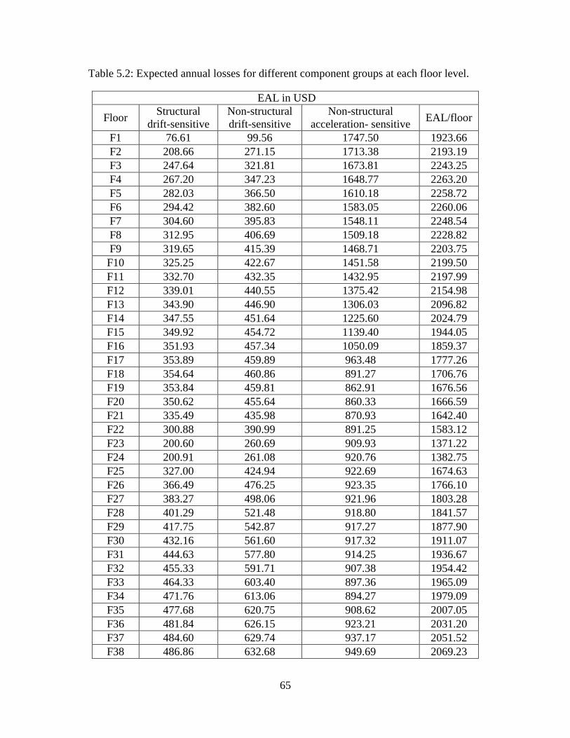
65
Table 5.2: Expected annual losses for different component groups at each floor level.
EAL in USD
Floor Structural
drift-sensitive
Non-structural
drift-sensitive
Non-structural
acceleration- sensitive EAL/floor
F1 76.61 99.56 1747.50 1923.66
F2 208.66 271.15 1713.38 2193.19
F3 247.64 321.81 1673.81 2243.25
F4 267.20 347.23 1648.77 2263.20
F5 282.03 366.50 1610.18 2258.72
F6 294.42 382.60 1583.05 2260.06
F7 304.60 395.83 1548.11 2248.54
F8 312.95 406.69 1509.18 2228.82
F9 319.65 415.39 1468.71 2203.75
F10 325.25 422.67 1451.58 2199.50
F11 332.70 432.35 1432.95 2197.99
F12 339.01 440.55 1375.42 2154.98
F13 343.90 446.90 1306.03 2096.82
F14 347.55 451.64 1225.60 2024.79
F15 349.92 454.72 1139.40 1944.05
F16 351.93 457.34 1050.09 1859.37
F17 353.89 459.89 963.48 1777.26
F18 354.64 460.86 891.27 1706.76
F19 353.84 459.81 862.91 1676.56
F20 350.62 455.64 860.33 1666.59
F21 335.49 435.98 870.93 1642.40
F22 300.88 390.99 891.25 1583.12
F23 200.60 260.69 909.93 1371.22
F24 200.91 261.08 920.76 1382.75
F25 327.00 424.94 922.69 1674.63
F26 366.49 476.25 923.35 1766.10
F27 383.27 498.06 921.96 1803.28
F28 401.29 521.48 918.80 1841.57
F29 417.75 542.87 917.27 1877.90
F30 432.16 561.60 917.32 1911.07
F31 444.63 577.80 914.25 1936.67
F32 455.33 591.71 907.38 1954.42
F33 464.33 603.40 897.36 1965.09
F34 471.76 613.06 894.27 1979.09
F35 477.68 620.75 908.62 2007.05
F36 481.84 626.15 923.21 2031.20
F37 484.60 629.74 937.17 2051.52
F38 486.86 632.68 949.69 2069.23
66
(Table 5.2 continued)
EAL in USD
Floor Structural
drift-sensitive
Non-structural
drift-sensitive
Non-structural
acceleration- sensitive EAL/floor
F39 488.22 634.44 949.79 2072.45
F40 488.34 634.60 911.17 2034.12
F41 487.51 633.52 870.47 1991.49
F42 485.77 631.26 854.21 1971.23
F43 483.32 628.08 879.37 1990.78
F44 477.81 620.92 901.22 1999.96
F45 470.73 611.71 916.57 1999.01
F46 460.74 598.74 912.33 1971.81
F47 427.19 555.14 905.84 1888.18
F48 322.03 418.49 905.59 1646.11
F49 318.88 414.38 903.87 1637.13
F50 438.41 569.72 911.29 1919.43
F51 475.96 618.51 891.74 1986.20
F52 512.58 666.10 849.97 2028.65
F53 536.34 696.98 802.21 2035.52
F54 554.14 720.10 749.27 2023.51
F55 568.75 739.10 707.19 2015.05
F56 580.51 754.38 685.92 2020.81
F57 589.69 766.31 667.42 2023.42
F58 599.28 778.77 659.92 2037.97
F59 609.82 792.47 652.49 2054.78
F60 612.27 795.65 639.59 2047.51
F61 612.87 796.42 656.70 2065.99
F62 611.51 794.66 677.96 2084.13
F63 607.87 789.93 693.89 2091.69
F64 602.46 782.91 746.54 2131.91
F65 595.57 773.95 807.30 2176.82
F66 587.13 762.97 849.92 2200.02
F67 577.08 749.92 886.85 2213.85
F68 565.60 735.00 920.46 2221.06
F69 552.64 718.16 976.93 2247.73
F70 538.22 699.43 1056.69 2294.35
F71 522.30 678.73 1132.70 2333.72
F72 504.49 655.59 1200.67 2360.74
F73 471.66 612.93 1254.77 2339.36
F74 391.68 508.99 1284.51 2185.17
Total 31979.23 41557.28 74781.34 148317.85
67
5.1.2 Multilayer Monte Carlo Simulation
In order to overcome the limitations of the analytical approach presented in the previous
section, the multilayer MCS technique was adopted in this study to estimate the DV’s statistical
characteristics (Conte and Zhang, 2007). In the case study, the multilayer MCS technique was used
to evaluate the MAR of exceeding a specified repair cost in USD of the target building following
a seismic event. Even though the strength of this technique is well recognized, implementing it
could be computationally costly since it requires a very high number of simulation samples to
obtain a convergence of the results.
5.1.2.1 Simulation of the hazard and the response
The hazard curve shown in Figure 5.1, approximated by the regression line in the
logarithmic scale given by eq. (5.1), was used for the simulation of the different values of the 5%-
damped spectral acceleration at the fundamental period of vibration of the structure. The maximum
acceleration that could possibly occur at the selected location is max 1( 5.4 , 5%) 2.130aS T s g
(see Figure 5.1), where g denotes the gravitational constant, whereas the minimum spectral
acceleration is the one below which no structural damage would appear. The value of the minimum
spectral acceleration was found to be min 1( 5.4 , 5%) 0.001aS T s g ; it was obtained by
decreasing gradually the value of aS until no damage, of any type, was observed. Therefore,
substituting these values in eq. (5.1), the MAR of exceedance corresponding to maximum and
minimum values of the spectral accelerations were obtained as:
4
max max
2
min min
1.15 10 eqk/year
3.00 10 eqk/year
a
a
S a
S a
S
S
(5.3)
The number of occurrences of earthquakes at the target location having an intensity level
between minaS and
maxaS was generated based on a Poisson process (Cornell, 1968) having a mean
68
rate min max . Then, for each of the earthquake occurrences, the value of Sa that was
generated and used in the MCS was obtained by a simple one-to-one mapping using a uniformly
distributed random variable U, and was calculated using eq. (2.11).
min 0min max
min max
1
min min max
0
k
aa a a a a
k
a
k SU P S s s S s
US
k
(5.4)
On the other hand, the median value of the EDP given an intensity level (i.e., EDP IM
), and
the standard deviation of the natural logarithm of the response ( EDP IM ) were evaluated at each
story level and fitted to the regression curve as described in section 5.1.1.2. Then, the response of
the structure, conditional on the intensity level, was generated by assuming that it follows a
lognormal distribution with median EDP IM and standard deviation EDP IM
.
5.1.2.2 Damage and loss assessment
Similar to the analytical solution, the damage analysis was performed using the story-based
approach and the fragility curves for the four damage states provided in HAZUS (FEMA, 2015a).
The median demand value of each damage state, as well as the corresponding standard deviation
of the natural logarithm of the demand, are given in Table 4.2. The fragility curves are depicted in
Figure 4.11 to Figure 4.13. For a given value of the EDP, i.e., MIDR or PFA at story j, the
probability that a group of components reaches each of the damage states was calculated using eq.
(2.16), then a randomly selected damage state weighted with the corresponding probability was
assigned to that group of components.
The losses corresponding to each of the damage states were randomly generated assuming
that they are lognormally distributed with mean values given in Table 4.3 and a COV equal to
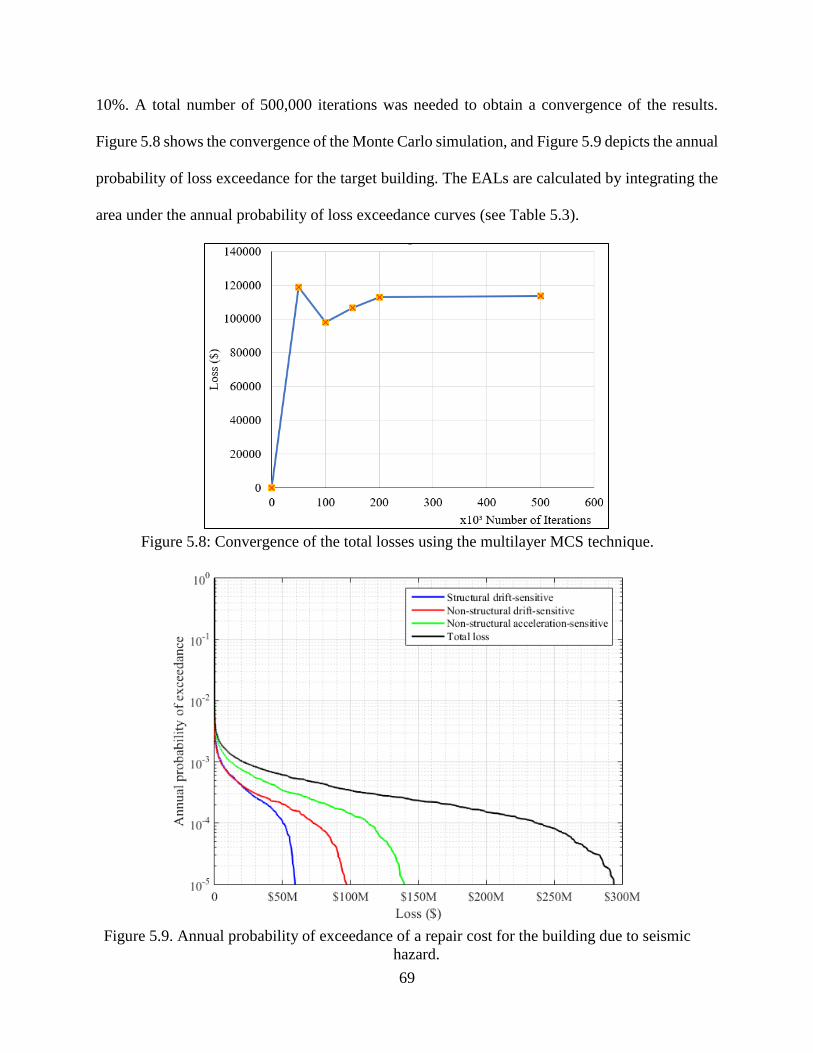
69
10%. A total number of 500,000 iterations was needed to obtain a convergence of the results.
Figure 5.8 shows the convergence of the Monte Carlo simulation, and Figure 5.9 depicts the annual
probability of loss exceedance for the target building. The EALs are calculated by integrating the
area under the annual probability of loss exceedance curves (see Table 5.3).
Figure 5.8: Convergence of the total losses using the multilayer MCS technique.
Figure 5.9. Annual probability of exceedance of a repair cost for the building due to seismic
hazard.
70
Table 5.3: Expected annual losses for different component groups at each floor level.
EAL in USD
Floor Structural
drift-sensitive
Non-structural
drift-sensitive
Non-structural
acceleration- sensitive EAL/floor
F1 19.56 17.53 1486.08 1523.16
F2 125.08 130.74 1532.97 1788.80
F3 153.17 167.95 1454.58 1775.71
F4 169.80 198.90 1402.40 1771.09
F5 193.20 197.72 1344.76 1735.67
F6 205.59 235.64 1344.51 1785.74
F7 213.30 219.03 1452.65 1884.98
F8 220.54 237.44 1256.86 1714.83
F9 235.84 258.38 1269.18 1763.40
F10 236.28 255.64 1239.44 1731.35
F11 236.20 271.88 1174.00 1682.08
F12 241.18 286.77 1194.22 1722.16
F13 237.43 283.88 1135.23 1656.54
F14 247.32 294.20 991.28 1532.81
F15 266.09 301.38 912.95 1480.43
F16 273.41 290.79 871.33 1435.53
F17 271.68 309.95 743.25 1324.88
F18 268.78 313.55 653.89 1236.21
F19 261.72 283.59 663.31 1208.61
F20 256.37 288.45 675.42 1220.25
F21 245.96 290.98 688.41 1225.35
F22 206.43 224.57 654.10 1085.09
F23 106.45 101.17 733.58 941.20
F24 113.31 131.03 732.36 976.69
F25 235.45 268.98 726.26 1230.70
F26 269.22 325.14 647.55 1241.92
F27 289.84 335.62 666.22 1291.67
F28 314.72 363.99 680.14 1358.86
F29 321.16 371.80 618.67 1311.63
F30 344.21 393.73 658.23 1396.18
F31 355.55 391.45 675.73 1422.73
F32 359.75 420.50 702.08 1482.32
F33 375.43 443.65 675.30 1494.37
F34 376.57 451.18 645.10 1472.86
F35 387.79 469.07 661.67 1518.53
F36 377.88 458.80 691.34 1528.02
F37 393.15 470.73 698.71 1562.59
F38 402.41 496.72 725.47 1624.60
71
(Table 5.3 continued)
EAL in USD
Floor Structural
drift-sensitive
Non-structural
drift-sensitive
Non-structural
acceleration- sensitive EAL/floor
F39 392.47 483.58 705.83 1581.88
F40 388.77 504.79 646.14 1539.70
F41 408.81 464.44 623.61 1496.86
F42 388.05 450.18 609.98 1448.22
F43 396.77 452.26 646.67 1495.71
F44 383.03 463.02 668.59 1514.64
F45 374.21 443.38 670.33 1487.92
F46 363.25 451.79 690.07 1505.11
F47 331.50 406.20 701.24 1438.94
F48 222.40 251.27 671.71 1145.38
F49 225.30 258.96 672.76 1157.03
F50 346.43 427.98 717.60 1492.00
F51 380.38 460.19 717.40 1557.97
F52 431.38 533.23 628.61 1593.22
F53 441.66 548.06 568.99 1558.71
F54 453.56 550.22 507.99 1511.77
F55 460.02 592.31 488.62 1540.95
F56 482.49 560.01 409.89 1452.38
F57 497.42 619.25 426.80 1543.47
F58 521.37 635.23 395.82 1552.41
F59 517.84 633.00 432.61 1583.45
F60 519.09 642.18 432.17 1593.44
F61 535.63 642.05 444.16 1621.83
F62 517.26 653.33 439.26 1609.85
F63 520.81 640.73 461.68 1623.22
F64 501.80 617.53 499.09 1618.41
F65 501.62 624.05 555.43 1681.09
F66 513.12 651.55 660.34 1825.01
F67 494.16 587.17 689.86 1771.19
F68 473.28 584.76 674.43 1732.47
F69 463.80 570.19 772.25 1806.24
F70 456.12 534.49 892.60 1883.20
F71 447.81 537.72 914.57 1900.10
F72 420.98 504.67 923.19 1848.83
F73 382.15 460.20 1023.82 1866.16
F74 310.92 366.61 1065.01 1742.54
Total 25273.47 30059.10 58128.31 113460.88
72
By comparing the results reported in Table 5.2 and Table 5.3, it is observed that the
analytical solution overestimates the EALs by approximately 31% when compared to the MCS.
One reason of this overestimation is that the MCS technique takes into account the correlation
between the losses among stories, which reduces the values of EALs. Moreover, the losses due to
structural damage represent about 20% of the total losses incurred by the structure. This result
indicates that the use of a linear elastic model assumption can lead to inaccurate estimates of the
total losses. In particular, the damage of the drift-sensitive structural and non-structural
components are being underestimated, whereas the acceleration-sensitive losses are being
overestimated. Therefore, an inelastic model should be considered to calculate in a more accurate
manner the response of the structure when subjected to seismic forces, which could then be used
for a more accurate loss estimate. The analysis could be performed by using different procedures
available in the literature, e.g., nonlinear time history analysis or nonlinear static pushover analysis
(ASCE, 2013).
5.2 Wind loss assessment
The same procedure based on the multilayer MCS technique that was described in detail
in chapter 4 was also used to perform the wind-induced loss assessment of the target structure for
the new location of New Madrid, Missouri, where non-hurricane wind is the source of hazard. The
3-second wind speeds at 10 m above the ground level were collected from the IEM database (IEM,
2017) for the years 1997 to 2016. The annual 3-second wind speed maxima were extracted and
converted to 10-minute-averaged wind velocities using the time conversion coefficient ct = 0.67
(Lungu and Rackwitz, 2001). Since the historical data obtained from the IEM correspond a terrain
exposure category D as described in the ASCE-7-10 (ASCE, 2010), and assuming the structure is
located in an area characterized by a terrain exposure category B, the terrain exposure conversion
73
factor, ce, was taken equal to 0.84 (Lungu and Rackwitz, 2001). The 10-minute annual maxima
10minV were then fitted to a lognormal distribution, which provided a mean equal to 16.2 m/s and
a standard deviation equal to 2.9 m/s after verifying the goodness-of-fit with a 99% confidence
level.
The randomness in the wind direction was included in the analysis. The wind rose
indicating the percentage of time the wind blows from a certain direction in the closest town to the
target location for which data is available, i.e., St. Louis, MO, taken from the NOAA’s SAMSON
dataset for years between 1961 and 1991 is shown in Figure 5.10. Additionally, the roughness
length 0z was considered to be lognormally distributed with mean value of 0.1 m and a COV of
30% (Zhang et al., 2008).
Figure 5.10: Wind rose diagram, St. Louis, MO.
74
The turbulent winds in both along- and across-wind directions were modeled analytically
by the model described in Carassale and Solari (2006). As for the previous application example,
also in this case the wind model used for the analysis does not include the effect of vortex shedding
on the structural response. In fact, even for these lower wind speed values, the model proposed by
Liang et al. (2002) produced response results that are physically unacceptable (refer to
APPENDIX C for more details about the obtained results). The mathematical expressions of the
normalized one-sided PSD functions are given in eq. (4.5). Furthermore, the same six modes of
vibrations listed in Table 4.1 were considered in the structural analysis that was performed in the
frequency domain. Each of the modes of vibration was characterized by a structural damping ratio
randomly sampled from a lognormal distribution with mean 0.02 and COV of 0.4 (Petrini and
Ciampoli, 2012). The modal damping ratios were assumed to be statistically independent.
The aerodynamic coefficients CD and CL used to evaluate the interaction parameters, i.e.,
the forces applied at each story of the building, were assumed to be normally distributed as
described in section 4.2.3. The structural model was also assumed to be linear elastic at all stages
of the analysis. The one-sided PSD functions of the response in terms of displacements and
accelerations were obtained using eq. (4.17). These functions were then integrated with respect to
the frequency in order to evaluate the variances of the responses. The peak values of the responses
at each story level were then calculated using eq. (4.19) through (4.26).
The fragility curves shown in Figure 4.11, Figure 4.12, and Figure 4.13 of each component
group, whose parameters are listed in Table 4.2, were used to quantify the probability of exceeding
a damage state given the EDP value. Then, the repair cost of each component group using a story-
based approach was generated based on lognormal distributions with mean values summarized in
Table 4.3 and a COV of 10%. Moreover, the serviceability limit state expressed in terms of
business interruption due to excessive vibrations perceived by the building’s occupants was also
75
included in the losses’ estimation. For this purpose, the PFA was compared to the human
perception threshold assumed to be deterministically equal to 0.15 m/s² for office buildings
(Ciampoli and Petrini, 2012). The business interruption losses were then generated based on a
lognormal distribution with mean equal to 0.95$ per square foot of floor area and a COV equal to
10%. The same approach adopted to evaluate the losses due to business interruption resulting from
non-hurricane wind and described in section 4.2.6 was adopted also in this application example.
The correlation between the mean daily maximum wind speeds over a one-year period and the
maximum annual wind speeds was included in the calculations. Since the mean daily maximum
wind velocities as well as the annual maxima were considered to be lognormally distributed, the
corresponding normal distribution of the natural logarithm of the variables were used to generate
the correlated random values. Having the correlation coefficient ,
ln
X Y between two lognormal
random variables, e.g., X and Y , the correlation coefficient ln ,ln
n
X Y of the corresponding
normally distributed variables, lnX and lnY, was obtained using the following equation (Žerovnik
et al., 2013):
,
ln ,ln
ln ln
1ln 1
ln
n X Y X Y
X Y
X Y X Y
(5.5)
where denotes the mean value and the standard deviation, the superscripts (n) and (ln) denote
normal and lognormal respectively. The building was assumed to be entirely closed for one day if
the daily acceleration exceeded the acceleration threshold in at least half of the number of floors
of the building. The loss due to the damage of the pressure-sensitive components was also
calculated as explained in section 4.2.6. In order to accurately estimate the annual probability of
loss exceedance, which is the CDF function of the DV, 10,000 samples were generated.
76
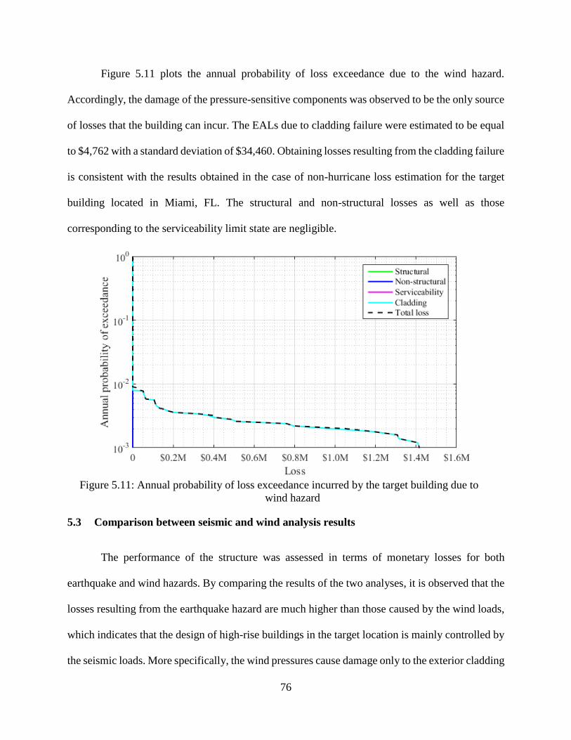
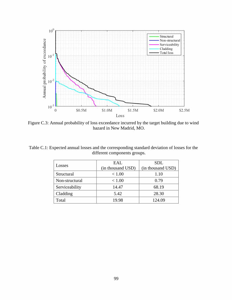
Figure 5.11 plots the annual probability of loss exceedance due to the wind hazard.
Accordingly, the damage of the pressure-sensitive components was observed to be the only source
of losses that the building can incur. The EALs due to cladding failure were estimated to be equal
to $4,762 with a standard deviation of $34,460. Obtaining losses resulting from the cladding failure
is consistent with the results obtained in the case of non-hurricane loss estimation for the target
building located in Miami, FL. The structural and non-structural losses as well as those
corresponding to the serviceability limit state are negligible.
Figure 5.11: Annual probability of loss exceedance incurred by the target building due to
wind hazard
5.3 Comparison between seismic and wind analysis results
The performance of the structure was assessed in terms of monetary losses for both
earthquake and wind hazards. By comparing the results of the two analyses, it is observed that the
losses resulting from the earthquake hazard are much higher than those caused by the wind loads,
which indicates that the design of high-rise buildings in the target location is mainly controlled by
the seismic loads. More specifically, the wind pressures cause damage only to the exterior cladding
77
of the structure while the damage to the structural and non-structural components is negligible.
This fact justifies the assumption of considering a linear elastic model in the structural analysis for
wind loads. By contrast, it is observed that structural drift-sensitive components are often damaged
by seismic loads, which implies the need for a more accurate loss analysis approach based on
nonlinear finite element analysis of the structure. In addition, the damage produced by the seismic
loads affects both (structural and non-structural) drift-sensitive components and acceleration-
sensitive components. Therefore, it is concluded that the wind losses could be reduced without
modifying the structural design by increasing the resistance to wind pressure of the cladding, e.g.,
by using annealed glass instead of regular glass; whereas the reduction of seismic losses can be
obtained only through a modification of the design and/or the addition of structural control
systems, such as tuned mass dampers, viscous dampers, or any other of the numerous seismic
mitigation techniques that have been extensively studied and explained in the literature (Kareem
et al., 1999; Ciampoli and Petrini, 2012). It is also observed that the selection of the appropriate
mitigation techniques for both wind and seismic actions should be decided based on a life-cycle
cost analysis (Frangopol et al., 1997; Unnikrishnan and Barbato, 2016), which can use the results
of the proposed wind and seismic loss analysis procedures as input data for estimating the changes
in expected losses.
78
6 CONCLUSIONS AND FUTURE WORK
Tropical cyclones and earthquakes are amongst the most disastrous natural phenomena that
affect human society and the built environment. The aftermath devastating damage includes not
only the loss of lives and displacement of thousands of people but also a tremendous economic
impact that could take years to be restituted. Therefore, it had been compulsory to introduce
structural design and assessment approaches that help reduce the risks entailed to hurricane and
seismic hazards. Performance-based engineering methodologies were developed and extensively
improved by the earthquake engineering community, whereas research studies relevant to
hurricane risks are still at initial stages.
In this study, the multi-hazard effect on high-rise buildings has been investigated using
probabilistic performance-based loss assessment methods by considering two different application
examples. In the first application example, the Performance-Based Hurricane Engineering (PBHE)
framework was extended and applied to a 74-story building located on the southeastern coast of
the United States, a region well-known for being frequently targeted by hurricanes. Because it
represents a consistent quantification of the performance when different hazards are investigated,
the expected annual losses in US dollars was chosen to be the decision variable. Different
uncertainties inherent to the problem were included in the analysis using the multilayer Monte
Carlo simulation technique. The hazard imposed by both hurricane and non-hurricane winds was
examined and direct losses of structural and non-structural components were evaluated. The
serviceability limit state as well as the pressure-induced damage were also included in the loss
analysis. It was observed that the losses due to the failure of cladding components are predominant
for high probabilities of exceedance, whereas the structural and non-structural damaged
components’ losses become predominant for lower probabilities of exceedance.
79
In the second application example, the same building considered before was assumed to be
located in the Central United States region, specifically in New Madrid (MO), which is a location
where both earthquake and wind hazards are active. Performance-based loss assessment methods
were also applied to calculate the expected annual losses. On one hand, the results of the seismic
effect obtained by applying the analytical procedure using a closed-form solution of the damage
and loss were compared to the ones calculated by means of the multilayer Monte Carlo simulation
technique. It was observed that the analytical solution overestimates the expected annual losses
mainly because it does not take into account the correlation among the different stories. On the
other hand, regarding the wind hazard, cladding failure was observed which consistently coincides
with what was obtained in the case of non-hurricane winds in Miami, FL. A comparison of the
losses caused by earthquake and wind hazards showed that the design of high-rise buildings in the
target location is controlled mainly by the seismic effects.
The research presented hereby is a first step towards a general approach to multi-hazard
performance-based engineering and uniform risk design for multiple hazards. It could be used to
establish a common ground to satisfy the objectives that owners/stakeholders would require in
developing new designs or retrofitting existing structures, and more importantly, optimize the
mitigation techniques for different hazards when acting at the same time. The following several
suggestions are given to propose future work needed to advance multi-hazard design
methodologies and applications based on the work presented in this thesis:
(1) During a hurricane event, the sources of hazard are not only limited to high wind speeds.
The multi-hazard nature of hurricanes combines the storm surge, the windborne debris and
heavy rainfall along with the wind. While the storm surge has impact on lower parts of
buildings, the other hazards can affect the entire structure. In addition, the level of damage
80
depends also on the interaction among these sources. Therefore, additional research is
needed in this direction in order to assess the performance of high-rise buildings subjected
to all the aspects of the hurricane hazard.
(2) In the case studies presented in this thesis, the structural analysis for wind loading was
performed in the frequency domain using a linear elastic model assumption. Future work
might need to take into account the nonlinear behavior of the structure as well as carry out
the calculations in the time domain and validate the results with full-scale measure of
performance during real events. Some possible methods available in the literature started
in this direction by introducing the wind incremental dynamic analysis to evaluate the
nonlinear time-history response of the structure.
(3) Available data is indicating that the hurricane surging activity might be caused by global
warming and climate change. Further investigations are required to validate the potential
effect of climate change on hurricane hazards, and how the impact on structural losses
would be modified.
(4) Performance-based engineering methods generally use fragility curves to estimate the
damage state for different structural and non-structural components. However, while the
research on fragility curves for earthquake loading is quite developed, significant more
work is needed to develop appropriate fragility curves for wind and hurricane effects.
(5) Previous studies showed that properly defining the intensity measure of the hazard increase
the accuracy of the loss assessment. Therefore, advanced and more complex models of IMs
including the interaction among hazard sources may have to be developed and probed for
high-rise structures.
81
(6) Simplified analysis procedures used to evaluate the nonlinear time-history responses of the
structure subjected to long duration hurricane events may be a potential area of research in
future studies.
(7) Different techniques of mitigation should be investigated to find their effectiveness under
different hazards and develop a selection method for multi-hazard conditions.
82
BIBLIOGRAPHY
ASCE (2010) Minimum Design Loads for Buildings and Other Structures. ASCE/SEI Standard 7-
10.
ASCE (2013) Seismic Evaluation and Retrofit of Existing Buildings. ASCE/SEI Standard 41-13.
Aslani, H. and Miranda, E. (2005) ‘Probabilistic earthquake loss estimation and loss
disaggregation in buildings’. Stanford University Stanford, CA.
ATC-40, A. T. C. (1996) Seismic evaluation and retrofit of concrete buildings, Vol 1. Applied
Technology Council, Redwood City, CA.
Augusti, G. and Ciampoli, M. (2008) ‘Performance-based design in risk assessment and
reduction’, Probabilistic Engineering Mechanics. Elsevier, 23(4), pp. 496–508.
Baker, J. W. (2008) ‘An introduction to Probabilistic Seismic Hazard Analysis (PSHA)’,