Multi-hypothesis Motion Planning for Visual Object Tracking

Haifeng Gong†, Jack Sim†, Maxim Likhachev‡, Jianbo Shi†† GRASP Lab, University of Pennsylvania

‡ Robotics Institute, Carnegie Mellon Universityhfgong@seas.upenn.edu, {jiwoong, jshi}@cis.upenn.edu, maxim@cs.cmu.edu

AbstractIn this paper, we propose a long-term motion model for

visual object tracking. In crowded street scenes, persistentocclusions are a frequent challenge for tracking algorithmand a robust, long-term motion model could help in thesesituations. Motivated by progresses in robot motion plan-ning, we propose to construct a set of ‘plausible’ plans foreach person, which are composed of multiple long-term mo-tion prediction hypotheses that do not include redundan-cies, unnecessary loops or collisions with other objects.Constructing plausible plan is the key step in utilizing mo-tion planning in object tracking, which has not been fullyinvestigate in robot motion planning. We propose a novelmethod of efficiently constructing disjoint plans in differenthomotopy classes, based on winding numbers and windingangles of planned paths around all obstacles. As the goalscan be specified by winding numbers and winding angles,we can avoid redundant plans in the same homotopy classand multiple whirls or loops around a single obstacle.

We test our algorithm on a challenging, real-worlddataset, and compare our algorithm with Linear TrajectoryAvoidance and a simplified linear planning model. We findthat our algorithm outperforms both algorithms in most se-quences.

1. IntroductionIn crowded street scenes, frequent occlusions, combined

with appearance changes, lead to ambiguous data associ-ation or ‘drifting’ in tracking. Many of these occlusionscould be dealt with using a long-term motion model. Mo-tivated by progresses in robot motion planning, we pro-pose to construct a set of ‘plausible’ plans for each person,which are composed of multi-hypotheses for motion predic-tion without redundancies, unnecessary loops or collisionswith other objects. Constructing ‘plausible’ plans is the keyproperty desired by visual object tracking but has not beenfully investigated in robot motion planning, which focuseson figuring out the most efficient path. We introduce a novelmethod of efficiently constructing disjoint plans in different

homotopy classes, based on winding numbers and windingangles of planned paths around all obstacles. As the goalscan be specified by winding numbers and winding angles,we avoid redundant plans in the same homotopy class ormultiple whirls and loops around a single obstacle, evenwith obstacles of varying different sizes and shapes.

There are two key factors distinguishing our motionmodel from traditional motion models. First, we explic-itly model pedestrian trajectories as goal-directed obstacle-avoiding paths using multiple hypotheses. Second, wecreate more flexible and realistic hypotheses for possiblepedestrian trajectories than others; simpler models of dy-namic social behavior [10] are limited in expressive powerbecause they use single hypotheses and short-term predic-tions.

For each person, our planner maintains multiple hy-potheses for future paths as they move in the environment,creating a ‘virtual simulation’ of intended pedestrian mo-tion. When a person is visible, we track them, and use theirtrajectory to narrow down the set of plausible goals/plannedpaths. When a person becomes occluded, we create multi-ple hypotheses that predict their re-appearance based on theplausible set of goals/planned paths provided by the plan-ner. Figure 1 illustrates this process.

We apply our motion model on batch-mode tracklets as-sociation, where we model, in the tracklet matching cost,agreement between goal-oriented motion plans. We test ourmethod on data collected from a car mounted with a stereocamera pair driven across an urban city.

2. Related WorkWhen multiple objects have a similar appearance, or

when occlusion happens and appearance features are cor-rupted, better motion model can improve tracking. Re-cently, object-interaction based motion models have at-tracted much attention. The most similar approaches to ourmethod are those of [6] and [9, 10]. Helbing et al[6] intro-duced a dynamic social behavior model for simulating peo-ple behavior. They model the velocities and accelerationsof people in crowds using three terms: 1) a term describing

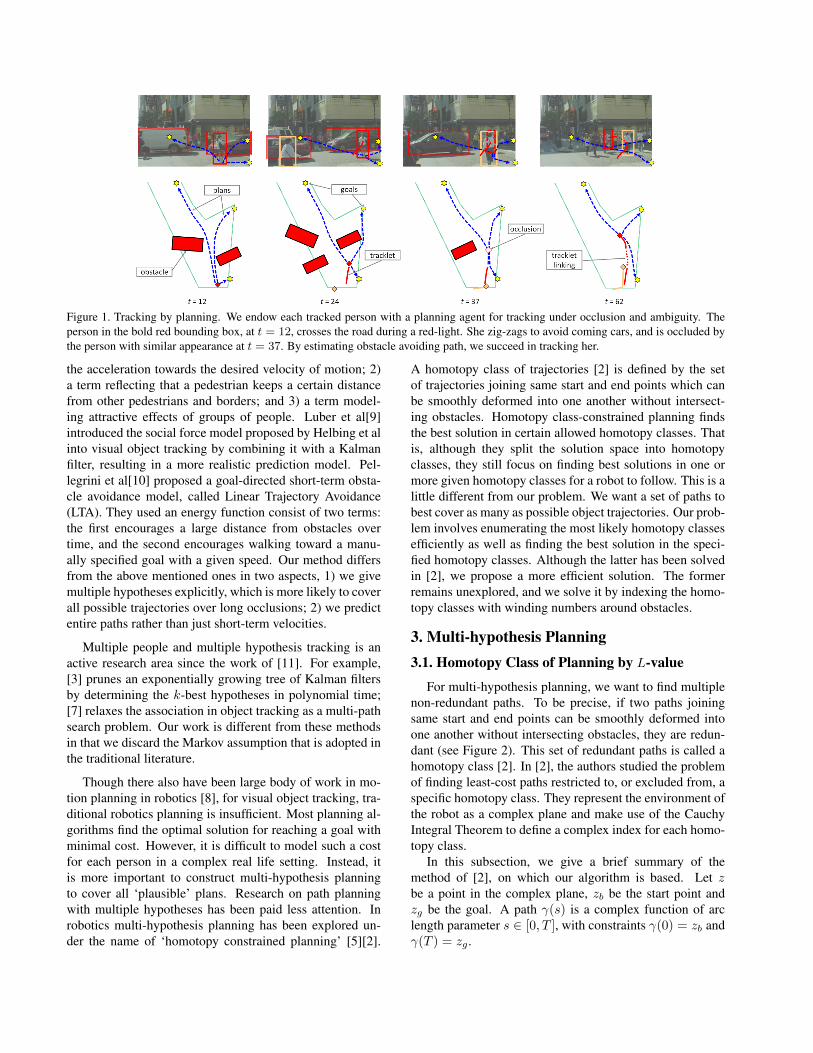
Figure 1. Tracking by planning. We endow each tracked person with a planning agent for tracking under occlusion and ambiguity. Theperson in the bold red bounding box, at t = 12, crosses the road during a red-light. She zig-zags to avoid coming cars, and is occluded bythe person with similar appearance at t = 37. By estimating obstacle avoiding path, we succeed in tracking her.

the acceleration towards the desired velocity of motion; 2)a term reflecting that a pedestrian keeps a certain distancefrom other pedestrians and borders; and 3) a term model-ing attractive effects of groups of people. Luber et al[9]introduced the social force model proposed by Helbing et alinto visual object tracking by combining it with a Kalmanfilter, resulting in a more realistic prediction model. Pel-legrini et al[10] proposed a goal-directed short-term obsta-cle avoidance model, called Linear Trajectory Avoidance(LTA). They used an energy function consist of two terms:the first encourages a large distance from obstacles overtime, and the second encourages walking toward a manu-ally specified goal with a given speed. Our method differsfrom the above mentioned ones in two aspects, 1) we givemultiple hypotheses explicitly, which is more likely to coverall possible trajectories over long occlusions; 2) we predictentire paths rather than just short-term velocities.

Multiple people and multiple hypothesis tracking is anactive research area since the work of [11]. For example,[3] prunes an exponentially growing tree of Kalman filtersby determining the k-best hypotheses in polynomial time;[7] relaxes the association in object tracking as a multi-pathsearch problem. Our work is different from these methodsin that we discard the Markov assumption that is adopted inthe traditional literature.

Though there also have been large body of work in mo-tion planning in robotics [8], for visual object tracking, tra-ditional robotics planning is insufficient. Most planning al-gorithms find the optimal solution for reaching a goal withminimal cost. However, it is difficult to model such a costfor each person in a complex real life setting. Instead, itis more important to construct multi-hypothesis planningto cover all ‘plausible’ plans. Research on path planningwith multiple hypotheses has been paid less attention. Inrobotics multi-hypothesis planning has been explored un-der the name of ‘homotopy constrained planning’ [5][2].

A homotopy class of trajectories [2] is defined by the setof trajectories joining same start and end points which canbe smoothly deformed into one another without intersect-ing obstacles. Homotopy class-constrained planning findsthe best solution in certain allowed homotopy classes. Thatis, although they split the solution space into homotopyclasses, they still focus on finding best solutions in one ormore given homotopy classes for a robot to follow. This is alittle different from our problem. We want a set of paths tobest cover as many as possible object trajectories. Our prob-lem involves enumerating the most likely homotopy classesefficiently as well as finding the best solution in the speci-fied homotopy classes. Although the latter has been solvedin [2], we propose a more efficient solution. The formerremains unexplored, and we solve it by indexing the homo-topy classes with winding numbers around obstacles.

3. Multi-hypothesis Planning3.1. Homotopy Class of Planning by L-value

For multi-hypothesis planning, we want to find multiplenon-redundant paths. To be precise, if two paths joiningsame start and end points can be smoothly deformed intoone another without intersecting obstacles, they are redun-dant (see Figure 2). This set of redundant paths is called ahomotopy class [2]. In [2], the authors studied the problemof finding least-cost paths restricted to, or excluded from, aspecific homotopy class. They represent the environment ofthe robot as a complex plane and make use of the CauchyIntegral Theorem to define a complex index for each homo-topy class.

In this subsection, we give a brief summary of themethod of [2], on which our algorithm is based. Let zbe a point in the complex plane, zb be the start point andzg be the goal. A path γ(s) is a complex function of arclength parameter s ∈ [0, T ], with constraints γ(0) = zb andγ(T ) = zg .

(a) Good plans

zb

zg

O1

O2

γ1

γ 2

γ 3

(b) Redundant plans

zb

zg

O1

O2

γ4

γ5

γ 6

γ 7

(c) Looped plan

zb

zg

O1

O2

γ 8

Figure 2. Examples of plausible plans and bad plans. O1 and O2

are two obstacles. γi are possible paths. zb and zg are the startpoint and goal respectively. (a) A set of good plans in differenthomotopy classes that have no unnecessary loops. (b) Two groupsof redundant plans: γ4 and γ5 belong to the same homotopy class,as do γ6 and γ7. (c) A path makes an unnecessary loop aroundobstacle O1. [2] can efficiently avoid bad plans like (b) by us-ing homotopy classes, but it cannot avoid the bad plans like (c)because it uses a simple complex number to index the homotopyclasses, which contains no information about loops. [2] enumer-ates all plans in all homotopy classes in the order of path costs.Assume that plain arc length is used as the cost, γ3 is the first tobe found, then γ2. Because γ8 is shorter than γ1, it is found next.[2] will make a couple of loops before reaching the next plausibleplan γ1.

To distinguish different homotopy classes, a complex ob-stacle marker function is defined as

F (z) =f0(z)

(z − ζ1)(z − ζ2) · · · (z − ζN )(1)

where f0(z) is a complex Holomorphic function and ζi isa point in the area covered by obstacle i in the complexplane. Using the Cauchy Integral Theorem, they showedthat two trajectories γ1(s) and γ2(s) connecting the samepair of points lie in the same holotopy class if and only if∫

γ1

F (z)dz =

∫γ2

F (z)dz (2)

given the assumption that f0(z) meets certain conditions.Therefore they use the L-value, defined as

L(γ) =

∫γ

F (z)dz (3)

to index homotopy classes. Note that although the L-valueis a continuous complex number, it only has discrete num-ber of possible values, given start point and goal.

Starting from a standard graph based planning config-uration, each vertex is augmented with multiple L-values,and becomes multiple vertices to form an augmented graph.Goals of different homotopy classes are different nodes inthis graph. The edges of the original graph are augmentedsimilarly with the increments of L-values. As such, stan-dard graph search algorithm can be used to find the shortestpath from the start point to the goal in a specified homotopyclass.

However, one cannot directly apply [2] for person track-ing:

1. When obstacles differ greatly in size, [2] performs poorlyin enumerating all the homotopy classes of plans. Their al-gorithm will focus on finding shortest paths with multipleloops around small obstacles before finding a path around theother side of a larger obstacle. This occurs because althoughtheir L-value can distinguish one homotopy class from otherones, it cannot carry other necessary information such as howmany loops a homotopy class contains. The authors suggestdiscarding smaller obstacles to overcome this problem. Thissuggestion is not acceptable in street scene tracking, wherepeople and cars are dynamic obstacles and have differentsizes. We cannot discard all people and consider only carsas obstacles. Figure 2 shows details about this point.

2. Obstacle marker function (1) must be carefully chosen fornumeric stability of L-values in real-world applications.

3. Their representation of state space is an infinite augmentedgraph. This occurs because that the L-value does not recordnumber of loops around the obstacle, and so has to allow infi-nite number of them. However, in real-world visual tracking,it is better to keep the search space finite.

We propose replacing L-value with a more informativeindex, that incorporates the number of loops around obsta-cles. This allow us to screen out any paths with many loops,which are unlikely to be the paths that people actually take.

3.2. From L-value to winding numbers

Following [2], we use the complex plane to describe theconfiguration space, i.e., ground and obstacles. Let us con-sider the L-value of a plan γ with respect to a single obsta-cle,

L =

∫γ

f(z)

z − z0dz (4)

where z0 is a point on the obstacle and f(z) can be anycomplex holomorphic function such that f(z0) 6= 0. L-values for a single obstacle must be in the discrete set of

{k ∗ 2πif(z0) + L0 : k ∈ Z}, (5)

where L0 is the L-value of the path from start point to goalat right side with no loop. Thus we can use k to distinguishhomotopy classes with respect to one obstacle which we callwinding number. For a plausible path, the values of k willlikely be 0 or −1, meaning ‘go-right’ or ‘go-left’ aroundthe obstacle. When k > 0, it indicates a path to the right ofthe obstacle that includes k loops around it. Similarly k <−1 indicates a path to the left of the obstacle that includes−k− 1 loops around it. In most cases, a plausible path willhave k ∈ {−1, 0}. Though for an obstacle or environmentwith irregular shape, the plausible path may has k < −1 ork > 0, in street scenes, we can hardly meet this situation.Therefore, we only consider k ∈ {−1, 0} as plausible inimplementation.

By letting ki be the k-value associated with the i-th ob-stacle, we can denote a homotopy class with respect to all

L = L0 − 4πif(z0) L = L0 − 2πif(z0) L = L0 L = L0 + 2πif(z0)k = −2 k = −1 k = 0 k = 1

∆θ = −3π ∆θ = −1π ∆θ = π ∆θ = 3π

1 1 1 1

1 1 1 1

Figure 3. Winding numbers and winding angles for one obstacle.First row, L-values. Second row, k-values. Third row, windingangles. Fourth row, example plans. Fifth row, more example plans.One can see that k > 0 or k < −1 indicates that there are loopsaround obstacles.

obstacles as an integer vector (vector of winding numbers,or k-vector)

k = (k1, k2, · · · , kN )T . (6)

Theorem 1. Two trajectories γ1 and γ2 with k-vectors k1

and k2 connecting the same points lie in the same homotopyclass if and only if k1 = k2.

Proof. if-clause: If k1 = k2, then L-values for all obstaclesare same, which means no obstacle is enclosed by the closedcontour formed by γ1 and γ2, following Theorem 1 in [2].Therefore, they lie in the same homotopy class. only-if-clause: If they lie in the same homotopy class, then theyenclose no obstacle, and therefore have same value in eachentry of their k-vectors.

Given a start point, a goal, and a set of obstacles, a one-to-one map can be established between the set of all homo-topy classes and the set of vectors of winding numbers. Thetheorem above states that vectors of winding numbers give acomplete description of the topology of feasible trajectoriesgiven an environment, a starting location, and goal.

3.3. From winding numbers to winding angles

In Eq. (4), we simply choose f(z) = 1 to be a constant.Given a path γ, if we write it in parametric form,

γ(s) = z0 + r(s) exp[iθ(s)] (7)

where s ∈ [0, T ] is arc length parameter, Eq. (4) can becomputed in closed form as

L = log r(T )− log r(0) + i[θ(T )− θ(0)], (8)

where the real part is constant for all possible paths γ withgiven start point and goal since r(0) = ‖z0 − zb‖ andr(T ) = ‖z0 − zg‖. The imaginary part

∆θ = θ(T )− θ(0) = ∆θ0 + 2kπ (9)

may differ by 2kπ, where k is also a winding number. Wecall ∆θ the winding angle of γ with respect to obstacle z0.Each path has a vector of winding angles with respect toall obstacles, ∆Θ = (∆θ1,∆θ2, · · · ,∆θN )T . Now, we canbuild our algorithm using winding angles directly, and donot need to consider L any more. See Figure 3 for examplesof winding numbers and winding angles.

3.4. Augmented Graph

Like [2], we use a graph based search algorithm. Webegin with neighborhood graph G, in which each grid pointon ground not occupied by an obstacle is a vertex, and eachpair of neighboring points are connected by an edge. Edgeweights are the costs of moving from one vertex to another.If we simply use path length as the cost, the shortest pathon this graph is the shortest path in the configuration spacesubject to no collisions. Each vertex in G is represented byits coordinate on ground z.

We augment this graph with winding angle to create anaugmented graph G. That is, we equip both vertices withwinding angles and edges with increments of winding an-gles. We can choose a set of possible vectors of wind-ing numbers K = {ki : i = 1, · · · , |K|}, in which |K|is the number of elements in K. If we choose 3 obsta-cles, we have |K| = 23 = 8, because for each obsta-cles, we have 2 choices of k ∈ {−1, 0}. Then, for eachvertex z in G, we have a set of vectors of winding anglesAz = {∆Θi

z : i = 1, · · · , |K|}, each of which correspondsto a winding number vector in K through Eq. (9). A vertexof the augmented graph G is represented by (z,∆Θi

z), thatis, the pair of each z and each of its winding angle vector∆Θi

z . If the number of vertices ofG is |G|, then the numberof vertices in G is |K| × |G|. Let e be the edge connectingtwo vertices z and z′ in the original graphG. The edge has afixed winding angle vector, ∆Θe. For the vertices (z,∆Θi

z)and (z′,∆Θi′

z′), we connect them if ∆Θi′

z′ = ∆Θiz + ∆Θe.

In the augmented graph, a goal is split into multiple verticesaccording to winding angle vector. See Figure 4 for moreexplanation.

The graph weights are defined in the following way.Given an environment with static and dynamic obstacles,we compute distance transformations of both a static obsta-cle map and a dynamic obstacle map. Let Dst and Ddyn

be the two distance transformations. We define a vertexweight map as W (z) = α0 + α1Dst(z) + α2Ddyn(z),where αj are weights that provide a trade-off between thethree terms. The weight of an edge e connecting z andz′ is defined as the average of the weights of the ver-tices it connects, multiplied by the distance between them,W (e) = 1

2{W (z) +W (z′)}‖z − z′‖.We use Dijkstra’s algorithm to search the augmented

graph. If too many obstacles are present, we select keyobstacles by first finding the shortest path in the original

a b c

def

O 1 O 2

a b c

def

O 1 O 2

α1 α2

α3

α4α5

α2:4

2π

−α1:5

a b c

def

a b c

def

a b c

def

a b c

def

k = (0, 0)

k = (0,−1)

k = (−1, 0)

k = (−1,−1)

b of (0, 1)a of (1, 1)

f of (−1,−2) e of (0,−2)

a of (1, 0)

f of (−2,−1)

b of (−1, 1)a of (0, 1)

f of (−2,−2) e of (−1,−2)

Figure 4. An example of augmented graph. Top box left, an exam-ple graph, with 6 nodes and 2 obstacles. a is the start point and d isthe goal. Top box right, the winding angles on edges. Bottom box,the augmented graph, with four k vectors. Each k correspond to alayer with 6 nodes marked by a shaded panel, that is, each node issplit into 4 in the augmented graph. From a in the first layer, thereis a shortest path to d in each of the layers. The shortest paths froma in k = (0, 0) to d in k = (0, 0) and k = (−1, 0) are shown inbold blue.

neighborhood graph G, then keeping the obstacles close tothe shortest path as key obstacles. Only the key obstaclesare considered for computing winding numbers.

4. Tracking by PlanningWe test our motion model in a batchmode tracking by

detection framework. During tracking, when a person ispartially or fully occluded, we estimate his position by plan-ning. Tracking a person in the visible state leads to a shorttrajectory that we call a tracklet. A conservative thresholdis used to terminate the trajectory when the tracking scorebecomes too low. After termination, the same person maybe picked up again by the detection algorithm, and trackedto produce associated tracklets. After tracklets are obtained,we can link them using both appearance and planning con-sistency.

4.1. Criteria for tracklets linking by planning

We defer the discussion of person detection and initialtracking until Section 4.3. For now, we assume that we havea set of tracklets T = {F1, · · · , FNTr

}, where Fi is the i-th tracklet, and NTr is the total number of tracklets. Eachtracklet is described by Fi = (ti0, t

i1,x

iti0, · · · ,xi

ti1), where

ti0 is the start time of Fi, ti1 is the end time of Fi and xit is theobject position at time t. Note that xit is defined in a fixed

3D world coordinate system defined by the initial camera.We first measure the people’s positions in the stereo imageframe, and map it to a fixed 3D world frame using the ego-motion estimation of the camera.

We then link and extend these tracklets, T , into completetrajectories, using the ‘estimated’ partial/full occlusion po-sition to explain away the ‘gap’ formed by the tracklets. LetLi,j be the indicator of linking i-th and j-th tracklet:

Li,j =

{1 Fi → Fj0 otherwise . (10)

To link tracklets into plausible goal-directed obstacle-avoiding paths, we design the following criterion for track-ing:

maxL

ε(L) =∑

i,j:Li,j=1

[SApp(i, j) + αSPlan(i, j)]− β|L|

(11)where SApp(i, j) measures appearance similarity betweentracklets Fi and Fj , SPlan(i, j) measures 1) how consis-tent Fi and Fj are with a plausible goal directed path;and 2) how partial occlusion in the gap can be explainedby appearance of Fi and Fj . We introduce α to tradeoff the two scores and β 6= 0 to prevent aggressive link-ing. The criterion (11) is subject to the following con-straints: Li,j ∈ {0, 1},

∑i Li,j 6 1,

∑j Li,j 6 1, and

Li,j = 0,∀(i, j) ∈ InvalidSet, where InvalidSet is used toexclude those links that indicates impossibly large speeds,too long gaps or time back-tracking. We seek an approxi-mate solution using Linear Programming.

4.2. Planning score

The planning score is given by finding the best plannedpath to fill the gap between tracklet i and j. The best pathis compatible with tracklet i and tracklet j geometrically,and allows possible partial matches by appearance duringocclusions. We use the following score: SPlan(i, j) =maxr∈paths−Dist(r, Fi)−Dist(r, Fj) + SOccl(Fi, Fj , r),where Dist(r, Fi) is the distance between path r and track-let Fi and SOccl(Fi, Fj , r) is the score for picking up thepartial occlusions along the gap. To reduce computation,we prune paths whose costs are higher than the minimalone above a threshold.

We compute the distance between a tracklet and plannedpath as follows. First, we shorten the tracklet by keepingonly the last M frames of Fi and first M frames of Fj ,giving the shortened tracklets F ′i and F ′j . Let x1, · · · , xMbe the tracked positions in F ′i or F ′j , and let l be the arclength of the shortened tracklet. Let p be the point on thepath r which is nearest to the start point of F ′i or F ′j . Usingp as start point, we can obtain an arc on the path r withlength l, which results in a shortened path r′. Finally, wedivide r′ into M − 1 segments uniformly, to obtain M end

points: r′1, · · · , r′M . We compute the distance Dist(r, Fi) =∑m ‖xm − r′m‖2.We find possible partial matches (by appearance) during

occlusions, to compute SOccl(Fi, Fj , r), which is definedby the score of two appearance models applied to the hallu-cinated trajectory bridging the gap. Given the path r, whichdoes not connect Fi and Fj perfectly, we first compute thehallucinated trajectory connecting Fi and Fj by a diffusionequation and project it to both cameras to pick up possiblepartial matches during occlusions. The diffusion equationuses the ends of Fi and Fj as boundary conditions, and thedifferences of the adjacent points on the planned paths asguided gradients.

4.3. Appearance Feature

Adaptive appearance model. For a pedestrian, we di-vide his image patch into three parts: head, torso and legs.Using a part based representation allows us to reason un-der partial occlusion. For each part k at time t, we col-lect the color histogram using 8 × 8 × 8 bins, denoted bypt(k), and we also collect the histogram of surroundingbackground, denoted by qt(k). We use simple color fea-ture instead of more advanced shape features for simplicityand computation efficiency. The histograms are collectedusing subsampling. We maintain running means of the his-tograms as an object model: ft = (1 − α) ∗ ft−1 + α ∗ pt,bt = (1 − α) ∗ bt−1 + α ∗ qt. Denote Modelt = (ft,bt)the object appearance model.

Tracklet creation. We use a detector based on [4] todetect peoples and cars in the current frame. To track aperson in frame t + 1 given the models of previous frame,Modelt, we measure two scores — Consistent Score (S1) toensure that it is similar to foreground appearance model ftand different from bt, and Contrast Score (S2) to ensure thatthe foreground is different from its surroundings in currentframe. They are defined as follows; S1(Modelt,pt+1) =12

∑k

∑bin pt+1(k) log ft(k)

bt(k)+ 1

2

∑ft(k) log pt+1(k)

bt+1(k), and

S2(Modelt,pt+1) =∑k KL{pt+1(k)‖qt+1(k)} =∑

k

∑bin pt+1(k) log pt+1(k)

qt+1(k).

Appearance score. The appearance score in Eq. (11)is obtained by testing the appearance model of tracklet i onmodel of tracklet j and vice-versa.

5. ExperimentsTo test our algorithm we have collected a video from a

moving vehicle in an urban city. The stereo images werecollected at 1024 × 768 resolution and 6 FPS. We have asystem for people detection (based on [4]), 3D scene lay-out/goal estimation, and camera ego-motion computation.The ground plane at the first frame of each sequences wascalibrated and propagated over time using the ego-motiontransformations. We estimated building planes and ground

Figure 5. Top: tracking with linear linking. It drifts after occlusion.Middle: tracking with planning. We are able to pick up the entiretrajectory of a pedestrian, despite the long occlusion. Bottom, topview of tracking with planning. The brown balls are current po-sitions, the red curves are trajectories, the bold black curve is theselected plan, the blue curves are other plans, gray squares arepossible goals. Black squares and rectangle are obstacles at plan-ning time. Note that we plan in advance, therefore, the obstaclesare other objects a few frames ago. Video frames are cropped forclarity. Better viewed in color.

plane in each frame and intersected them to get street sidelines. The goals are estimated by intersecting the street sidelines, plus infinity points along the street. We only trackpeople, but detect cars using [4]. When planning for a spec-ified object, other objects are regarded as obstacles.

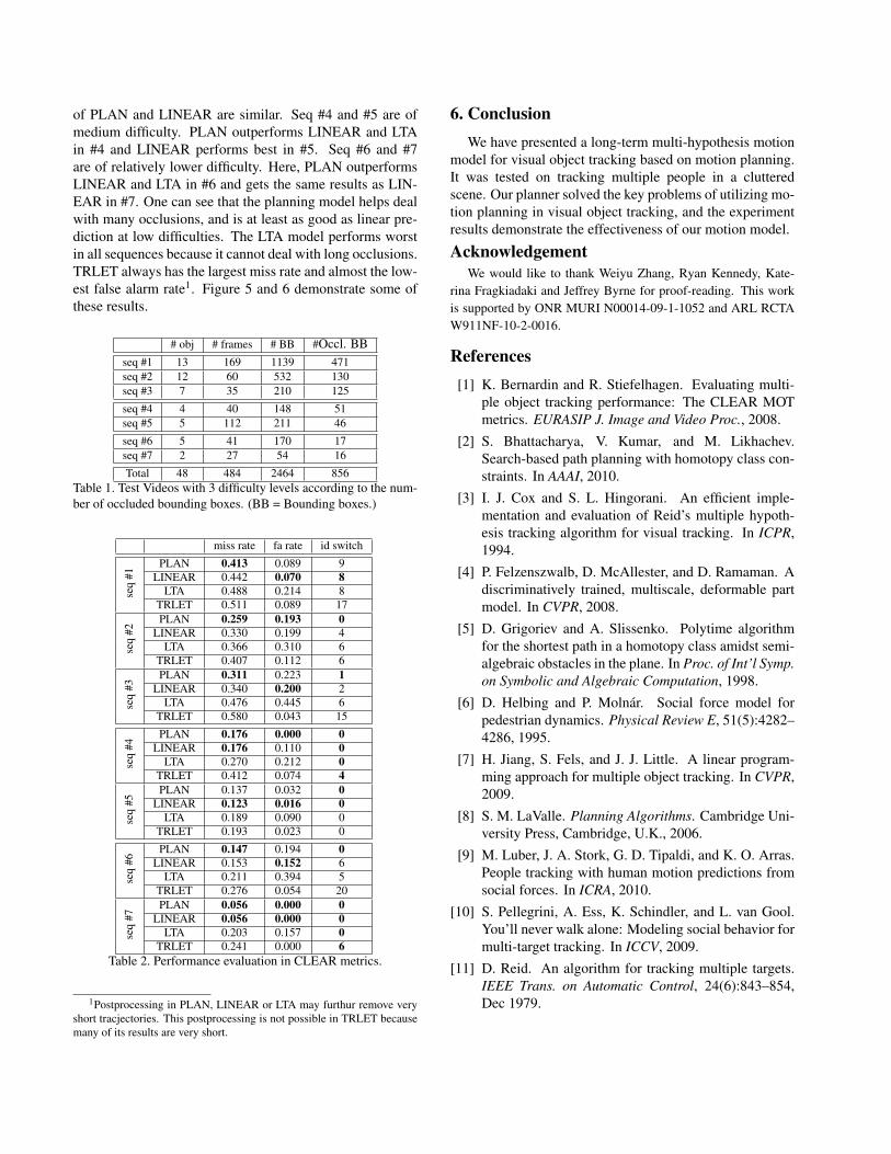
We have picked 7 sequences which contains multiplepeople, and have interesting interactions and occlusions.Details of all sequences are shown in Table 1. There aretotal of 48 people in all the sequences. Many of thesepeople cannot be tracked through the entirety of the se-quence, because of the high occlusion rates. For compar-ison, we implement two baselines, 1) (LINEAR) trackletlinking without planning, that is, using a straight line as aplan to try to link the gaps, and 2) (LTA) Linear TrajectoryAvoidance[10]. In the implementation of 1), we try straightline connection between all possible tracklet pairs, and pickthe possible partial occlusions in the gaps. In the imple-mentation of 2), we use LTA to predict a path from the endof one tracklet to the start of the other, and also pick up thepossible partial occlusions in the gaps. We also compute theperformace of our conservative tracklets (TRLET).

Table 2 shows the performance comparison in CLEARMetrics[1]. We use 3 metrics: false alarm rate, miss rate andnumber of identity switches. The false alarms are causedby false alarms in detection and wrong occluded boundingboxes drifting to background. The misses are caused bymisses in detection and failure to collect occluded bound-ing boxes. Note that we annotate the bounding boxes of anobject even if it is totally occluded.

We divide the sequences into 3 difficulties, based on thenumber of occlusions. Seq #1, #2 and #3 are the most dif-ficult ones. PLAN outperforms LINEAR and LTA in twoof them and for the extremely difficult Seq #1, the results

of PLAN and LINEAR are similar. Seq #4 and #5 are ofmedium difficulty. PLAN outperforms LINEAR and LTAin #4 and LINEAR performs best in #5. Seq #6 and #7are of relatively lower difficulty. Here, PLAN outperformsLINEAR and LTA in #6 and gets the same results as LIN-EAR in #7. One can see that the planning model helps dealwith many occlusions, and is at least as good as linear pre-diction at low difficulties. The LTA model performs worstin all sequences because it cannot deal with long occlusions.TRLET always has the largest miss rate and almost the low-est false alarm rate1. Figure 5 and 6 demonstrate some ofthese results.

# obj # frames # BB #Occl. BBseq #1 13 169 1139 471seq #2 12 60 532 130seq #3 7 35 210 125

seq #4 4 40 148 51seq #5 5 112 211 46

seq #6 5 41 170 17seq #7 2 27 54 16

Total 48 484 2464 856Table 1. Test Videos with 3 difficulty levels according to the num-ber of occluded bounding boxes. (BB = Bounding boxes.)

miss rate fa rate id switch

seq

#1

PLAN 0.413 0.089 9LINEAR 0.442 0.070 8

LTA 0.488 0.214 8TRLET 0.511 0.089 17

seq

#2

PLAN 0.259 0.193 0LINEAR 0.330 0.199 4

LTA 0.366 0.310 6TRLET 0.407 0.112 6

seq

#3

PLAN 0.311 0.223 1LINEAR 0.340 0.200 2

LTA 0.476 0.445 6TRLET 0.580 0.043 15

seq

#4

PLAN 0.176 0.000 0LINEAR 0.176 0.110 0

LTA 0.270 0.212 0TRLET 0.412 0.074 4

seq

#5

PLAN 0.137 0.032 0LINEAR 0.123 0.016 0

LTA 0.189 0.090 0TRLET 0.193 0.023 0

seq

#6

PLAN 0.147 0.194 0LINEAR 0.153 0.152 6

LTA 0.211 0.394 5TRLET 0.276 0.054 20

seq

#7

PLAN 0.056 0.000 0LINEAR 0.056 0.000 0

LTA 0.203 0.157 0TRLET 0.241 0.000 6

Table 2. Performance evaluation in CLEAR metrics.

1Postprocessing in PLAN, LINEAR or LTA may furthur remove veryshort tracjectories. This postprocessing is not possible in TRLET becausemany of its results are very short.

6. ConclusionWe have presented a long-term multi-hypothesis motion

model for visual object tracking based on motion planning.It was tested on tracking multiple people in a clutteredscene. Our planner solved the key problems of utilizing mo-tion planning in visual object tracking, and the experimentresults demonstrate the effectiveness of our motion model.

AcknowledgementWe would like to thank Weiyu Zhang, Ryan Kennedy, Kate-

rina Fragkiadaki and Jeffrey Byrne for proof-reading. This workis supported by ONR MURI N00014-09-1-1052 and ARL RCTAW911NF-10-2-0016.

References[1] K. Bernardin and R. Stiefelhagen. Evaluating multi-

ple object tracking performance: The CLEAR MOTmetrics. EURASIP J. Image and Video Proc., 2008.

[2] S. Bhattacharya, V. Kumar, and M. Likhachev.Search-based path planning with homotopy class con-straints. In AAAI, 2010.

[3] I. J. Cox and S. L. Hingorani. An efficient imple-mentation and evaluation of Reid’s multiple hypoth-esis tracking algorithm for visual tracking. In ICPR,1994.

[4] P. Felzenszwalb, D. McAllester, and D. Ramaman. Adiscriminatively trained, multiscale, deformable partmodel. In CVPR, 2008.

[5] D. Grigoriev and A. Slissenko. Polytime algorithmfor the shortest path in a homotopy class amidst semi-algebraic obstacles in the plane. In Proc. of Int’l Symp.on Symbolic and Algebraic Computation, 1998.

[6] D. Helbing and P. Molnar. Social force model forpedestrian dynamics. Physical Review E, 51(5):4282–4286, 1995.

[7] H. Jiang, S. Fels, and J. J. Little. A linear program-ming approach for multiple object tracking. In CVPR,2009.

[8] S. M. LaValle. Planning Algorithms. Cambridge Uni-versity Press, Cambridge, U.K., 2006.

[9] M. Luber, J. A. Stork, G. D. Tipaldi, and K. O. Arras.People tracking with human motion predictions fromsocial forces. In ICRA, 2010.

[10] S. Pellegrini, A. Ess, K. Schindler, and L. van Gool.You’ll never walk alone: Modeling social behavior formulti-target tracking. In ICCV, 2009.

[11] D. Reid. An algorithm for tracking multiple targets.IEEE Trans. on Automatic Control, 24(6):843–854,Dec 1979.

Figure 6. Image patches and bounding boxes over time. Each panel shows the bounding boxes of a pedestrian in two parts. The top partsshow the image patches of ground truth (1st row), PLAN results (2nd row) and LINEAR results (3rd row). The number on each box isthe frame number. They are trimmed on left or right for better visual effects. The bottom parts show video frames superimposed withbounding boxes. The magenta bounding boxes are current objects of interests. Yellow bounding boxes are other objects. The bold greenlines are the planned routes that the objects follow. The thinner green lines are other planned paths (after pruning) that are not followed bythe people. Seq 1 shows subsampled patches from a 154-frame trajectory. A girl in black is first occluded by a pole for about 25 frames(0∼24), then occluded by a girl in red for 15 frames (38∼53) and finally occluded by a truck for 5 frames (124∼128). PLAN covers almostthe whole trajectories, with some small drifts. LINEAR fails to link the two long occlusion. Seq 2, a woman is occluded for about 10frames, PLAN catches up after occlusion, and picks up correct partial occlusions; but LINEAR drifts away to a detection false alarm. Seq3, a man undergoes two short occlusions, is caught up by PLAN, but LINEAR and LTA terminate the trajectory too early. Video framesare cropped for clarity. Better viewed in color.