Multi-objective approach based on grammar-guided genetic programming for solving multiple instance...

ORIGINAL PAPER

Multi-objective approach based on grammar-guided geneticprogramming for solving multiple instance problems

Amelia Zafra • Sebastian Ventura

Published online: 8 December 2011

� Springer-Verlag 2011

Abstract Multiple instance learning (MIL) is considered

a generalization of traditional supervised learning which

deals with uncertainty in the information. Together with

the fact that, as in any other learning framework, the

classifier performance evaluation maintains a trade-off

relationship between different conflicting objectives, this

makes the classification task less straightforward. This

paper introduces a multi-objective proposal that works in a

MIL scenario to obtain well-distributed Pareto solutions to

multi-instance problems. The algorithm developed, Multi-

Objective Grammar Guided Genetic Programming for

Multiple Instances (MOG3P-MI), is based on grammar-

guided genetic programming, which is a robust tool for

classification. Thus, this proposal combines the advantages

of the grammar-guided genetic programming with benefits

provided by multi-objective approaches. First, a study of

multi-objective optimization for MIL is carried out. To do

this, three different extensions of MOG3P-MI are designed

and implemented and their performance is compared. This

study allows us on the one hand, to check the performance

of multi-objective techniques in this learning paradigm and

on the other hand, to determine the most appropriate evo-

lutionary process for MOG3P-MI. Then, MOG3P-MI is

compared with some of the most significant proposals

developed throughout the years in MIL. Computational

experiments show that MOG3P-MI often obtains consis-

tently better results than the other algorithms, achieving the

most accurate models. Moreover, the classifiers obtained

are very comprehensible.

Keywords Multiple instance learning � Multiple

objective learning � Grammar guided genetic

programming � Evolutionary rule learning

1 Introduction

Multiple instance learning (MIL), introduced by Dietterich

et al. (1997), is considered a special learning framework

which deals with the uncertainty of instance labels. This

learning framework extends traditional supervised learning

to problems with incomplete knowledge about the labels in

the training examples. Thus, in supervised learning, every

training instance is assigned a label that is discrete or has a

real-value. In comparison, in MIL, the labels are assigned

only to bags of instances and the labels for individual

instances are unknown. This learning framework has

expanded enormously in the last few years due to the great

number of applications for which it has been found to be

the most appropriate form of representation, achieving an

improvement over results obtained by traditional super-

vised learning. Some examples are: text categorization

(Andrews et al. 2002), content-based image retrieval (Pao

et al. 2008), image annotation (Yang et al. 2005), drug

activity prediction (Maron 1997), web index page recom-

mendation (Zhou et al. 2005; Zafra et al. 2009), semantic

video retrieval (Chen et al. 2009), video concept detection

(Gu et al. 2008; Gao 2008), pedestrian detection (Pang

et al. 2008), and the prediction of student performance

(Zafra et al. 2011). All these applications are based on

classification tasks. The problem of evaluating the quality

of a classifier, whether from the MIL perspective or in

A. Zafra � S. Ventura (&)

Department of Computer Science and Numerical Analysis,

University of Cordoba, Cordoba, Spain

e-mail: [email protected]

A. Zafra

e-mail: [email protected]

123

Soft Comput (2012) 16:955–977

DOI 10.1007/s00500-011-0794-0

traditional supervised learning, is naturally posed in multi-

objective problems with several contradictory objectives

that maintain a trade-off between them. That is, they

necessitate considering several conflicting objectives to be

optimized simultaneously and when one of them is opti-

mized the others reduce their value. In this context, it is

interesting to obtain the different non-dominated solutions

where the several objectives are more optimized at the

same time. In general, the different classification algo-

rithms usually attempt to optimize some validity measures

such as accuracy, comprehensibility, sensitivity, and

specificity.

The great variety of real-world decision problems that

necessitate considering several conflicting objectives to be

optimized simultaneously has made multi-objective opti-

mization very popular and there exists a large body of

literature devoted to multi-objective optimization for tra-

ditional supervised learning where nowadays still has very

recognition (Wu et al. 2011; Liao et al. 2011; Yang et al.

2011). However, we are unaware of multi-objective tech-

niques for classification MIL setting. All proposals to solve

this problem from an MIL perspective fail to take into

account the multi-objective problem and they obtain only

one optimal solution combining the different objectives to

obtain a high quality classifier. The main problem of these

techniques is that they obtain a single well-defined optimal

solution but these problems do not have a single solution:

rather, they have a set of non-comparable ones. These

solutions are known as efficient, nondominated or Pareto

optimal solutions, and the set of them is called the Pareto

Optimal Front (POF). None of these solutions can be

considered better than any other in the same set from the

point of view of the simultaneous optimization of multiple

objectives, all of them perform in the same way to solve the

problem. Therefore, in these problems, the major challenge

consists of generating the set of efficient solutions to

achieve an improvement of some objectives without sac-

rificing any other objective.

Our aim is to introduce a multiple objective proposal

which simultaneously optimizes different contradictory

objectives and provides the non-dominated solution set for

each problem. To do that, a multi-objective grammar gui-

ded genetic programming algorithm for MIL is developed

and it is called Multi-Objective Grammar-Guided Genetic

Programming for Multiple Instance Learning (MOG3P-

MI). The proposal is based on Grammar Guided Genetic

Programming (G3P) that generates rules in IF–THEN form

and evaluates the quality of each classifier according to two

conflicting quality indexes: sensitivity and specificity.

First, to evaluate the performance of the proposed

approach, we consider three different versions of MOG3P-

MI algorithm modifying the philosophy of its evolutionary

process. To do that, three different approaches based on

classic evolutionary multi-objective techniques frequently

used in literature in traditional supervised learning are

adapted and designed to work in the MIL framework. This

empirical study allows us to analyze the performance of

multi-objective techniques in MIL. Then, MOG3P-MI is

compared with the most representative techniques in MIL

designed over the years (specifically, 16 different proposals

are considered in this study). Computational experiments

show that our proposal is a robust algorithm which

achieves better results than the other previous techniques,

finding a balance between sensitivity and specificity and

yielding the most accurate models.

This paper is organized as follows. In Sect. 2, an over-

view of multi-instance and multi-objective learning

frameworks is given. Section 3 presents a description of the

approaches proposed. In Sect. 4, experiments and com-

parisons are carried out. Finally, conclusions and some

possible lines for future research are discussed in Sect. 5.

2 Preliminaries

This section gives the most important definitions in mul-

tiple objective optimization, developments carried out in

the framework of multiple instances learning, and the most

relevant studies in classification tasks using evolutionary

multi-objective techniques.

2.1 Multiple objective learning

The basic concepts related to multi-objective learning will

be introduced. Consider a multi-objective optimization

problem with p objectives where X denotes the finite set of

feasible solutions. We assume that each criterion has to be

maximized.

maximize ff1ðxÞ; f2ðxÞ; . . .; fpðxÞgsubject to x 2 X

�

We assume

• there are n decision variables x ¼ ðx1; x2; . . .; xnÞT ;• X � <n is the set of feasible solutions, i.e., decision

variables, defined by constraints,

• fi : X ! < are p conflicting objective functions,

• f ðxÞ ¼ ðf1ðxÞ; f2ðxÞ; . . .; fpðxÞÞT 2 <p is called an objec-

tive vector,

• Z ¼ f ðXÞ is called the criterion space, and

• z 2 Z are called criterion vectors.

Since, in general, a feasible solution that simultaneously

maximizes all the objective functions does not exist, the

concept of efficient or Pareto optimal solution is used in

this context. A feasible solution x� 2 X (and the corre-

sponding objective vector f ðx�Þ) is said to be efficient or

956 A. Zafra, S. Ventura

123

Pareto optimal for the problem if there does not exist any

other feasible solution x 2 X; such that fiðxÞ� fiðx�Þ for all

i ¼ 1; . . .; p with at least one j 2 1; . . .; p such that

fjðxÞ[ fjðx�Þ:The image of x�; z� ¼ f ðx�Þ; is said to be a non-domi-

nated vector. The set of all efficient solutions of the

problem is called the efficient set, and correspondingly, the

set of all the non-dominated vectors is called the non-

dominated set or Pareto Front. A feasible solution for the

problem ðx�Þ is said to be weakly efficient or weakly Pareto

Optimal if there does not exist any other feasible solution x

such that f ðxÞ[ f ðx�Þ: In this case, z� is said to be a weakly

non-dominated vector. Finally, a feasible solution x� for the

problem is said to be properly efficient or properly Pareto

optimal if it is efficient and the trade-offs between objec-

tives are bounded.

Also, the concepts of ideal and nadir values are relevant

in MOP. The ideal point is defined as z�i ¼ maxffiðxÞ j x 2Xg: It contains the best values that each objective function

can get in the POF. On the other hand, the worst values of

each objective function in the POF constitute a vector

known as a nadir point znad 2 <p with components

z�i ¼ min fiðxÞ j x 2 POF:

2.2 Learning techniques for multiple instance learning

The learning paradigm of multi-instance learning has found

great popularity in the machine learning (ML) community

and many proposals for classification (Dietterich et al.

1997), clustering (Zhang 2009) and regression (Ray 2001)

tasks have been studied. All of them optimize a combina-

tion of different objectives. Therefore, they do not obtain a

Pareto Front with the optimization of the different objec-

tives, rather they obtain a single solution which optimizes

composite objectives.

In MIL, classically the algorithms have been classified

into two categories. First, algorithms designed specifi-

cally to work in an MIL environment. In this category,

we find APR algorithms (Dietterich et al. 1997): these

algorithms attempt to find an APR by expanding or

shrinking a hyper-rectangle in the instance feature space

to maximize the number of instances from different

positive bags enclosed by the rectangle while minimizing

the number of instances from negative bags within the

rectangle. A bag was classified as positive if at least one

of its instances fell within the APR; otherwise, the bag

was classified as negative. Maron and Lozano (1997)

whose proposal came very soon after Dietterich’s,

developed a method called Diverse Density that is still

one of the most popular today. The interest this proposal

held can still be seen in how it is used combined with

other methods, e.g., with the expectation maximization

method, EM-DD (Wang 2000), and even recently there

are studies that propose extensions of it (Pao et al. 2008;

Xu et al. 2008).

The other category considers algorithms adapted from

the traditional supervised learning paradigm to perform

correctly in MIL. Thus, we can find that the most relevant

techniques in traditional supervised learning using single

instances have been adapted to MIL. In the following, we

present a review of the main methods developed. In the

lazy learning context, Wang and Zucker (2000) proposed

two alternatives, Citation-KNN and Bayesian-KNN, which

extend the k nearest-neighbour algorithm (KNN) to the

MIL context. With respect to decision trees and learning

rules, Chevaleyre and Zucker (2001) implemented ID3-MI

and RIPPER-MI, which are multi-instance versions of the

decision tree algorithm ID3 and rule learning algorithm

RIPPER, respectively. At that time, Ruffo (2000) presented

a multi-instance version of the C4.5 decision tree, which

was called RELIC. Later, Zhou et al. (2005) presented the

Fretcit-KNN algorithm, which is a variant of the Citation-

KNN. We can also find contributions which extend stan-

dard neural networks to MIL. Ramon and Raedt (2000)

presented a neural network framework for MIL. Following

their work, others have appeared, improving or extending

it. For instance, Zhou and Tang (2002) proposed BP-MIP, a

neural network-based multi-instance learner derived from

the traditional backpropagation neural network. An exten-

sion of this method adopting two different feature selection

techniques was proposed by Zhang and Zhou (2004). Other

interesting proposals of this paradigm are the works of

Zhang and Zhou (2006) and Chai and Yang (2007). The

support vector machine (SVM) has been another approach

adapted to the MIL framework. There are numerous pro-

posals for this approach: such as Gartner et al. (2002) and

Andrews et al. (2002), which adapted kernel methods to

work with MIL data by modifying the kernel distance

measures to handle sets. On the other hand, other works as

Chen and Wang (2004) and Chen et al. (2006) adapted

SVMs by modifying the form of the data rather than

changing the underlying SVM algorithms. Recently, other

works that use this approach include those of Mangasarian

and Wild (2008), Gu et al. (2008), and Lu et al. (2008).

The use of ensembles also has been considered in this

learning, the works of Xu and Frank (2004), Zhang and

Zhou (2005), and Zhou and Zhang (2007) are examples of

this paradigm. Finally, we can find multi-instance evolu-

tionary algorithms which adapt grammar-guided genetic

programming to this scenario (Zafra 2010), but from a

mono-objective perspective.

2.3 Classification system optimization

Multi-objective strategies are especially appropriate for

classification tasks because different measures taken to

Multi-objective approach based on G3P for MIL 957

123

evaluate the quality of the solutions are related, so if the

value of any of them is maximized, the value of the others

can be significantly reduced (Veldhuizen 2000). These

measurements involve the search for classification systems

that represent understandable, interesting and simple

descriptions of a specified class, even when that class has

few representative cases in the data. Multi-objective

metaheuristics can be used to produce different trade-offs

between confidence, coverage and complexity in the results

of classifiers.

A great variety of different methods have been devel-

oped for multi-objective optimization during the last few

years. Among them the multi-objective evolutionary

algorithms (MOEAs) have been a widely used approach to

confronting these types of problem (Coello et al. 2007).

The use of evolutionary algorithms (EAs) is mainly moti-

vated by the population-based nature of EAs which allow

the generation of several elements in the Pareto Optimal

Set in a single run. That is why, it is easy to find examples

of multi-objective techniques for evolutionary computation

on classification topics where significant advances in

results have been achieved (Shukla 2007; Tsang et al.

2007; Wee et al. 2009; Tan et al. 2009). Specifically, if we

evaluate its use in Genetic Programming (GP), we find that

its transfer to the multi-objective domain provides better

solutions than those obtained using standard GP in the

mono-objective domain, and with a lower computational

cost (Parrott et al. 2005; Mugambi 2003; Dehuri 2008).

3 Multi-objective grammar guided genetic

programming for MIL

G3P (Whigha 1995) is an extension of traditional GP

systems. G3P facilitates the efficient automatic discovery

of empirical laws providing a more systematic way to

handle typing. Moreover, the use of a context-free

grammar establishes a formal definition of the syntactical

restrictions. The motivation to include this paradigm is

on the one hand, the variable length solution represen-

tation which introduces a high flexibility in the solution

representation and on the other hand, the high efficiency

achieved both in obtaining classification rules with low

error rates, and in other tasks related to prediction, such

as feature selection and the generation of discriminant

functions (Chien et al. 2002; Kishore et al. 2000). With

respect to multi-objective strategies, the main motivation

to include them is, as indicated in Sect. 2.3, that they are

especially appropriate for classification tasks where it

is necessary to optimize two or more conflicting objec-

tives subject to certain constraints and also because

their use with GP has improved those obtained using

standard GP.

The most relevant aspects which have been taken into

account in the design of our proposal, such as individual

representation, genetic operators, and fitness function are

explained in detail next. Moreover, we describe the three

different evolutionary approaches that have been consid-

ered in our study resulting three different extensions called

MOG3P-MIðv1Þ; MOG3P-MIðv2Þ and MOG3P-MIðv3Þ: These

approaches follow the philosophy of well-known multi-

objective algorithms in traditional supervised learning.

Thus, the first one follows the evolutionary strategy of the

Strength Pareto Evolutionary Algorithm (SPEA2) (Zitzler

et al. 2001), the second one is based on the Non-dominated

Sorting Genetic Algorithm (NSGA2) (Deb et al. 2000) and

the third one on Multi-objective genetic local search

(MOGLS) (Jaszkiewicz 2003).

3.1 Individual representation

In our system, an individual is expressed by information in

the form of IF–THEN classification rules which provide a

natural extension to knowledge representation. The IF part

of the rule (antecedent) contains a logical combination of

conditions about the values of predicting attributes, and the

THEN part (consequent) contains the predicted class for

the concepts that satisfy the antecedent of the rule. This

rule determines if a bag should be considered positive (i.e.,

if it is an instance of the concept we want to represent) or

negative (if it is not). The scheme of the rules is seen in

expression 1.

If ðcondBðmÞÞ thenthe bag, m; represents the concept

that we want to learn.

Elsethe bag, m; does not represent the

concept that we want to learn:End-If

ð1Þ

where condB is a condition that is applied to the bag.

Following the Dietterich et al. (1997) hypothesis, condB

can be expressed as Eq. 2 where m is an example or bag, mi

is the ith instance of the bag m;V is the feature vectors of m

and VðmiÞ the feature vector of instance mi:

condBðmÞ ¼1; if 9VðmiÞ 2 m j condIðVðmiÞÞ ¼ 1

0; otherwise

�ð2Þ

The individuals’ genotypes that evolve in our system

correspond to the condition applied to instances (i.e.,

condI), while the phenotype represents the entire rule that

is applied to the bags (i.e., expression 1). The conditions of

the rule applied to instances ðcondIÞ are described

according to the language specified by a context-free

grammar ðGÞ which establishes a formal definition of the

syntactical restrictions of the problem to be solved and


123

allows of expressing the rule in a very natural way. The

grammar is defined by means of the next four elements:

G ¼X

N;X

T ; S;P� �

whereP

N \P

T ¼ ø;P

N is the alphabet of non terminal

symbols,P

T is the alphabet of terminal symbols, S is the

axiom and P is the set of productions written in Backus–Naur

form (BNF) (Knut 1964). Figure 1 shows the grammar used

to represent the antecedent of our rules which correspond to

the specification of condI and Fig. 2 shows the representation

of the genotype of an individual in our system.

3.2 Genetic operators

The process of generating new individuals in a given

generation of the evolutionary algorithm is carried out by

two operators, crossover and mutator, based on the pro-

posal of Whigham (1996). In this section, we briefly

describe their functioning. A interesting work about genetic

operators in multi-objective evolutionary optimization can

be consulted in Qian et al. (2011).

3.2.1 Crossover operator

This operator creates new rules by mixing the contents of

two parent rules. To do so, a non-terminal symbol is chosen

with a specific probability from among the available non-

terminal symbols in the grammar and two subtrees (one

from each parent) are selected whose roots coincide with

the same symbol selected or with a compatible symbol. To

reduce bloating, if either of the two offspring is too large, it

will be replaced by one of its parents. Specifically, the

crossover operator, given two individuals ðtree1 and tree2Þ;consists of the steps specified in Listing 1. The main fea-

tures of this operator are:

Fig. 1 Grammar used for representing individuals’ genotypes

Fig. 2 Representation of individual’s genotype


123

1. It avoids excessive growth in the size of the derivation

trees representing individuals (Couchet et al. 2006), a

problem well known as code bloat (Panait 2004).

2. It provides an appropriate balance between the ability of

exploration and exploitation of search space, preserving

the context in which subtrees appear in the parent trees.

3. It uses a list with the symbols which can be selected

and their probabilities can be specified. Thus, we can

increase or decrease the probability of modifying

certain symbols by other ones.

3.2.2 Mutation operator

This operator selects with a specific probability a symbol to

carry out the operation. Then, a node is chosen randomly

containing that symbol in the tree where the mutation is to

take place. If the node is a terminal node, it will be replaced

by another compatible terminal symbol. More precisely,

two nodes are compatible if they are derivations of

the same non-terminal. When the selected node is a non-

terminal symbol, the grammar is used to derive a new


123

subtree which replaces the subtree underneath that node. If

the new offspring is too large, it will be eliminated to avoid

having invalid individuals. Specifically, the mutation

operator given an individual ðtreeÞ performs the steps

specified in Listing 2.

The main features of this operator are:

1. It avoids an excessive growth in the size of the derivation

trees representing individuals (Couchet et al. 2006), a

problem well known as code bloat (Panait 2004).

2. It modifies individuals by changing simple compatible

terminal symbols between them. This allows us to

make small modifications when the population has

already converged.

3. It uses a list with the symbols which can be selected

and their probabilities can be specified. Thus, we can

increase or decrease the probability of modifying

certain symbols by other ones.

3.3 Fitness function

The fitness function is a measure of the effectiveness of the

classifier. There are several measures to evaluate different

components of the classifier and determine the quality of

each rule. We consider two widely accepted parameters for

characterizing models in classification problems: sensitiv-

ity (Se) and specificity (Sp) (Bojarczuk et al. 2000; Tan

et al. 2002). Sensitivity is the proportion of cases correctly

identified as meeting a certain condition and specificity is

the proportion of cases correctly identified as not meeting a

certain condition. Both are specified as follows:

sensitivity ¼ tptp þ fn

tp number of positive bags correctly identified:fn number of positive bags not correctly identified:

�


123

specificity ¼ tntn þ fp

tn number of negative bags correctly identified:fp number of negative bags not correctly identified:

�

We look for rules that maximize both sensitivity and

specificity at the same time. Nevertheless, there exists a

well-known trade-off between these two parameters

because they evaluate different and conflicting

characteristics in the classification process. Sensitivity

alone does not tell us how well the test predicts other

classes (i.e., the negative cases) and specificity alone does

not clarify how well the test recognizes positive cases. We

need to know both the sensitivity of the test for the class

and specificity for the other classes. In binary classification,

the trade-off between two measurements occurs because

when we increase the sensitivity value, the rule improves

the correct classification of positive objects, and it

normally produces a decrease in specificity because more

positive examples are accepted at the expense of also

accepting objects that belong to another class (negative

class). There is a similar scenario when we increase

specificity values at the expense of sensitivity values.

3.4 Evolutionary algorithms

Three different proposals are implemented according to the

previous specifications. With respect to the evolutionary

process, the idea is to extend three of the most widely used

and compared multi-objective evolutionary algorithms in

traditional supervised learning to MIL. A brief description

of the evolutionary process is described for each approach

considered. The algorithm finished when the number of

generations specified is researched or when an acceptable

solution is found. In our case, a solution is considered as

acceptable when it classifies correctly all examples of

training set.

3.4.1 MOG3P-MIðv1Þ Algorithm

The main steps of this algorithm are based on the prin-

ciples of the well-known Strength Pareto Evolutionary

Algorithm 2 (SPEA2) (Zitzler et al. 2001). The main

characteristics are: an external set (archive) is created for

storing primarily non-dominated solutions, the use of a

fitness value which takes into account how many indi-

viduals each individual dominates and is dominated by

and which is used to decide what dominated solutions

will take part in the population when the number of non-

dominated solutions is smaller than the archive size and a

truncation operator to reduce the number of non-domi-

nated solutions when this number is higher than the

population size. This operator considers that the smallest

distance to the other solutions will be removed from the

set to produce greater diversity. The general outline of

this algorithm is shown in Listing 3.


123


The main steps of this algorithm are based on the well-

known Non-Dominated Sorting Genetic Algorithm

(NSGA2) (Deb et al. 2000). The main differences between

the previous algorithm and this one is the elitism-preser-

vation operation. MOG3P-MIðv2Þ uses dominance ranking

to classify the population into a number of layers, so that

the first layer is the best layer in the population. The

archive is created based on the order of ranking layers: the

best rank being selected first. If the number of individuals

in the archive is smaller than the population size, the next

layer will be taken into account and so on. In this case, a

truncation operator based on the crowding distance is

applied if, on adding a layer the number of individuals in

the archive exceeds the initial population size. This oper-

ator removes the individual with the smallest crowding

distance. The crowding distance of a solution is defined as

the averaged total of objective-value differences between

two adjacent solutions of that solution. To calculate this,

the population is sorted according to each objective, thus

the adjacent solutions are localized and infinite values are

assigned to boundary solutions. The general outline of this

algorithm is shown in Listing 4.


The main steps of this algorithm are based on the well-

known multi-objective genetic local search (MOGLS)

(Jaszkiewicz 2003). MOG3P-MIðv3Þ uses genetic local

search (GLS) and implements the idea of the simulta-

neous optimization of all weighted Tchebycheff scalar-

izing functions by random choice of the utility function

optimized in each iteration. That is, in each iteration, it

tries to improve the value of a randomly selected utility

function. A single iteration in this algorithm consists of a

single recombination of a pair of solutions and the off-

spring are then used as a starting point for a local

search. The general outline of this algorithm is shown in

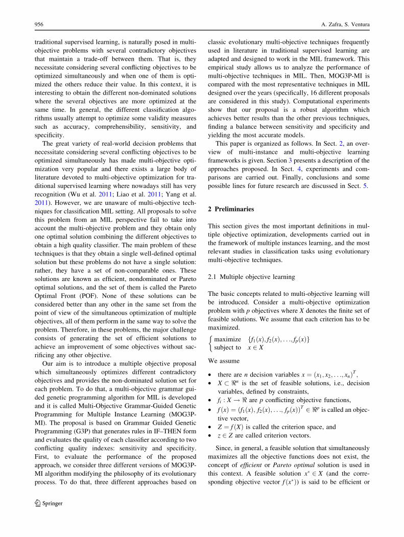
Listing 5.


123

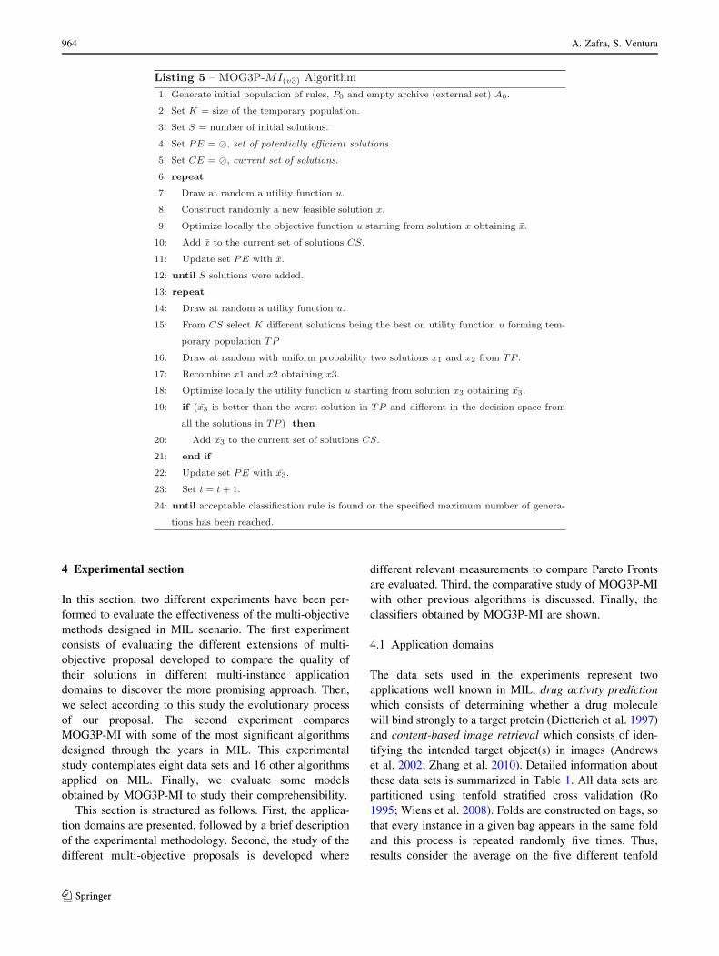
4 Experimental section

In this section, two different experiments have been per-

formed to evaluate the effectiveness of the multi-objective

methods designed in MIL scenario. The first experiment

consists of evaluating the different extensions of multi-

objective proposal developed to compare the quality of

their solutions in different multi-instance application

domains to discover the more promising approach. Then,

we select according to this study the evolutionary process

of our proposal. The second experiment compares

MOG3P-MI with some of the most significant algorithms

designed through the years in MIL. This experimental

study contemplates eight data sets and 16 other algorithms

applied on MIL. Finally, we evaluate some models

obtained by MOG3P-MI to study their comprehensibility.

This section is structured as follows. First, the applica-

tion domains are presented, followed by a brief description

of the experimental methodology. Second, the study of the

different multi-objective proposals is developed where

different relevant measurements to compare Pareto Fronts

are evaluated. Third, the comparative study of MOG3P-MI

with other previous algorithms is discussed. Finally, the

classifiers obtained by MOG3P-MI are shown.

4.1 Application domains

The data sets used in the experiments represent two

applications well known in MIL, drug activity prediction

which consists of determining whether a drug molecule

will bind strongly to a target protein (Dietterich et al. 1997)

and content-based image retrieval which consists of iden-

tifying the intended target object(s) in images (Andrews

et al. 2002; Zhang et al. 2010). Detailed information about

these data sets is summarized in Table 1. All data sets are

partitioned using tenfold stratified cross validation (Ro

1995; Wiens et al. 2008). Folds are constructed on bags, so

that every instance in a given bag appears in the same fold

and this process is repeated randomly five times. Thus,

results consider the average on the five different tenfold


123

stratified cross validation. This procedure is carried out to

guarantee the reliability of results. All these partitions of each

data set are available at http://www.uco.es/grupos/kdis/

momil to facilitate future comparisons.

4.2 Experimental setup

The designed multi-objective algorithms have been

implemented in the JCLEC software (Ventura et al. 2007)

with the main parameters as shown in Table 2. All

experiments are repeated with ten different seeds and the

average results are reported in the result tables.

The algorithms used for comparison are obtained from the

WEKA workbench (Witten 1999) and JCLEC framework

(Ventura et al. 2007) and consider some of the most signif-

icant proposals in this research field. The configuration of

these methods is based on an experimental study considering

different configurations and then selecting the best config-

uration in each case. The results of this experiment can be

consulted in http://www.uco.es/grupos/kdis/mil.

4.3 Comparison of multi-objective strategies

In this section, a comparative study between the multi-

objective proposals is performed. First, we analyse the

Pareto Front obtained by each proposal and then we eval-

uate the quality of the final classifier that would be selected

in each case.

4.3.1 Analysis of the Pareto Front quality

of multi-objective strategies

The outcome of the multi-objective algorithms used is a non-

dominated solution set (an approximation of the Pareto

Optimal Front). A sample of the Pareto Front obtained in one

execution with each method can be found in Figs. 3, 4 and 5.

An analysis of the quality of these approximation sets is

made to compare the different multi-objective techniques.

Many performance measures which evaluate different

characteristics have been proposed; some of the most pop-

ular such as spacing, hypervolume, and coverage of sets

(Coello et al. 2007) are analysed in this work and their

average results on the different data sets studied are shown in

Table 3. The spacing (Coello et al. 2007) metric describes

the spread of the non-dominated set. According to the results

shown, the non-dominated front of MOG3P-MIðv2Þ has all

solutions more equally spaced than the other algorithms

because the value is the lowest one. Another measurement

considered is the hypervolume indicator (Coello et al.

2007), defined as the area of coverage of a non-dominated

Table 1 General information about data sets

Data set ID Bags Attributes Instances Average

bag sizePos Neg Total

Musk1 Mus1 47 45 92 166 476 5.17

Musk2 Mus2 39 63 102 166 6,598 64.69

Mutagenesis-atoms MutA 125 63 188 10 1,618 8.61

Mutagenesis-bonds MutB 125 63 188 16 3,995 21.25

Mutagenesis-chains MutC 125 63 188 24 5,349 28.45

Elephant ImgE 100 100 200 230 1,391 6.96

Tiger ImgT 100 100 200 230 1,220 6.10

Fox ImgF 100 100 200 230 1,320 6.60

Table 2 Parameters used for multi-objective algorithms

Parameter MOG3P-MIðv1Þ MOG3P-MIðv2Þ MOG3P-MIðv3Þ

Population size 1,000 1,000 80

External population size 100 100 50

Temporal population size – – 50

Number of generations 150 150 5,000

Crossover probability 95% 95% 100%

Mutation probability 80% 80% –

Parent selector Tournament selector (size = 2) Tournament selector (size = 2) Random selector

(With repetition) (Without repetition)

Maximum tree depth 50 50 50


123

http://www.uco.es/grupos/kdis/momil

http://www.uco.es/grupos/kdis/momil

http://www.uco.es/grupos/kdis/mil

set with respect to the objective space. The results show that

the non-dominated solutions of MOG3P-MIðv2Þ obtain the

highest values, therefore its POF covers more area than the

other techniques’ POFs. Finally, the coverage of two sets

(Coello et al. 2007) is evaluated. This measurement can be

termed the relative coverage comparison of two sets. The

results show that MOG3P-MIðv2Þ obtains the highest values

when it is compared with the other techniques, then by

definition the outcomes of MOG3P-MIðv2Þ dominate the

outcomes of the other algorithms. Taking into account, all

the results obtained in the different metrics, it could be said

that MOG3P-MIðv2Þ achieves a better approximation of the

POF than the other techniques.

4.3.2 Analysis of solution quality of multi-objective

strategies

In this section, we analyse the average values of accuracy,

sensitivity and specificity for the different data sets. To do

this, in our proposal, the solution (classifier) of Pareto

0

0,2

0,4

0,6

0,8

1S

peci

ficity

Sensitivity

(a) Mutagenesis Atoms

0

0,2

0,4

0,6

0,8

1

Spe

cific

ity

Sensitivity

(b) Mutagenesis Bonds

0

0,2

0,4

0,6

0,8

1

Spe

cific

ity

Sensitivity

(c) Mutagenesis Chains

0

0,2

0,4

0,6

0,8

1

Spe

cific

ity

Sensitivity

(d) Elephant

0

0,2

0,4

0,6

0,8

1

Spe

cific

ity

Sensitivity

(e) Tiger

0

0,2

0,4

0,6

0,8

1

0 0,2 0,4 0,6 0,8 1 0 0,2 0,4 0,6 0,8 1 0 0,2 0,4 0,6 0,8 1

0 0,2 0,4 0,6 0,8 1 0 0,2 0,4 0,6 0,8 1 0 0,2 0,4 0,6 0,8 1

Spe

cific

ity

Sensitivity

(f) Fox

Fig. 3 Pareto Front of MOG3P-MIðv1Þ for the different learning problems

0

0,2

0,4

0,6

0,8

1

Spe

cific

ity

Sensitivity


0

0,2

0,4

0,6

0,8

1

Spe

cific

ity

Sensitivity


0

0,2

0,4

0,6

0,8

1

Spe

cific

ity

Sensitivity


0

0,2

0,4

0,6

0,8

1

Spe

cific

ity

Sensitivity

(d) Elephant

0

0,2

0,4

0,6

0,8

1

Spe

cific

ity

Sensitivity

(e) Tiger

0

0,2

0,4

0,6

0,8

1

0 0,2 0,4 0,6 0,8 1 0 0,2 0,4 0,6 0,8 1 0 0,2 0,4 0,6 0,8 1

0 0,2 0,4 0,6 0,8 1 0 0,2 0,4 0,6 0,8 1 0 0,2 0,4 0,6 0,8 1

Spe

cific

ity

Sensitivity

(f) Fox



123

Front obtained in training set with the best balance in

sensitivity and specificity measurements is selected to be

evaluated on test partition and then its results are used in

this comparison. Formally, the procedure carried out is

shown in Fig. 6.

The average results of the accuracy (Acc), sensitivity

(Se) and specificity (Sp) values for each measurement are

shown for each data set in Table 4. At first glance,

MOG3P-MIðv2Þ seems to obtain better results in the most of

data sets and the different metrics compared with the other

versions. However, to evaluate the differences between the

algorithms more precisely, a statistical test is carried out.

Specifically, Wilcoxon signed-rank test (Demsa 2006) is

used. This is a non-parametric test recommended in

Demsar (2006) and Garcia et al. (2010) which allows us to

address the question of whether there are significant dif-

ferences between the accuracy, sensitivity and specificity

values obtained by the three proposals. To do this, the null

hypothesis maintains that there are no significant differ-

ences between the values of the three metrics obtained by

the different techniques while the alternative hypothesis

asserts that there are. This test evaluates the differences in

performance comparing the proposals two by two. Thus,

three difference comparisons are made for each measure-

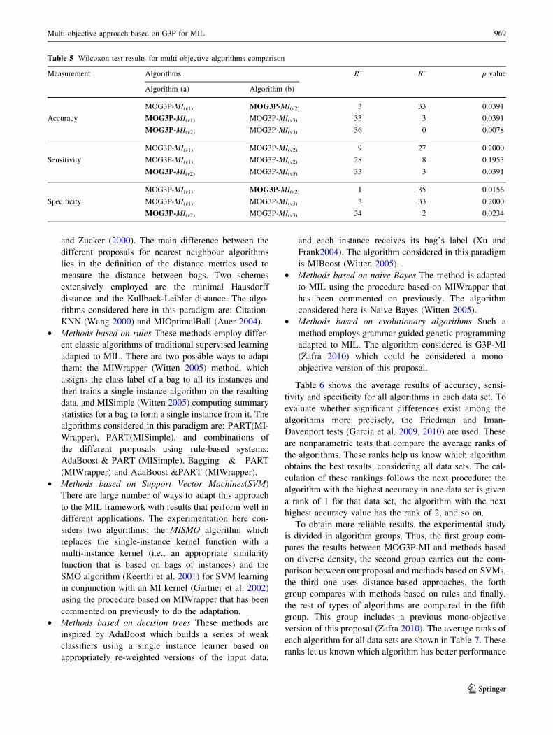
ment (accuracy, sensitivity and specificity). Table 5 shows

the results obtained in all possible comparisons among the

three algorithms considered in the study for the different

metrics. In all cases, we use a 95% confidence level. Thus,

we mark in bold the winner algorithm in each row when the

Wilcoxon test asserts that there are significant differences

between the results of two algorithms.

Regarding accuracy metric, the best algorithm is the

MOG3P-MIðv2Þ that obtains a considerable higher value of

ranks. This means that this version obtains a better

accuracy values in a greater number of data sets. In the

same table, it is shown the p-value that allows to reject

the null hypothesis with a confidence level of 95% and

we can determine that MOG3P-MIðv2Þ overcomes the

results in the comparison with MOG3P-MIðv1Þ and with

MOG3P-MIðv3Þ being a better proposal than the others.

0

0,2

0,4

0,6

0,8

1S

peci

ficity

Sensitivity


0

0,2

0,4

0,6

0,8

1

Spe

cific

ity

Sensitivity


0

0,2

0,4

0,6

0,8

1

Spe

cific

ity

Sensitivity


0

0,2

0,4

0,6

0,8

1

Spe

cific

ity

Sensitivity

(d) Elephant

0

0,2

0,4

0,6

0,8

1

Spe

cific

ity

Sensitivity

(e) Tiger

0

0,2

0,4

0,6

0,8

1

0 0,2 0,4 0,6 0,8 1 0 0,2 0,4 0,6 0,8 1 0 0,2 0,4 0,6 0,8 1

0 0,2 0,4 0,6 0,8 1 0 0,2 0,4 0,6 0,8 1 0 0,2 0,4 0,6 0,8 1

Spe

cific

ity

Sensitivity

(f) Fox


Table 3 Analysis of quality of POFs considering average values for all data sets studied

Algorithm Hypervolume (HV) Spacing (S) Two set coverage (CS)

MOG3P-MIðv3Þ 0.844516 0.016428 CS(MOG3P-MIðv3Þ; MOG3P-MIðv2Þ) 0.357052

CS(MOG3P-MIðv3Þ;MOG3P-MIðv1Þ) 0.430090

MOG3P-MIðv2Þ 0.890730 0.007682 CS(MOG3P-MIðv2Þ;MOG3P-MIðv3Þ) 0.722344


MOG3P-MIðv1Þ 0.872553 0.012290 CS(MOG3P-MIðv1Þ;MOG3P-MIðv3Þ) 0.508293



123

Moreover, MOG3P-MIðv1Þ also obtains better results than

MOG3P-MIðv3Þ in the comparison two to two.

A similar analysis can be made for the other metrics:

sensitivity and specificity. With respect to sensitivity

metric, MOG3P-MIðv2Þ obtains better results than MOG3P-

MIðv3Þ; but there are no significant differences between the

results obtained compared to MOG3P-MIðv1Þ: However,

MOG3P-MIðv2Þ achieves a higher rank sum than MOG3P-

MIðv1Þ: Finally, in the specificity values, again, MOG3P-

MIðv2Þ overcomes the other two models in the individual

comparisons.

In conclusion, MOG3P-MIðv2Þ achieves the best

approximation to Pareto Optimal Front according to any of

the measurements evaluated and the best accuracy, sensi-

tivity and specificity values in the different data sets.

Moreover, Wilcoxon test determines that its results are

better than both versions compared one to one for accu-

racy and specificity measurements and it is better than

MOG3P-MIðv3Þ for sensitivity values. Therefore, finally our

proposal, MOG3P-MI, will be based on this evolutionary

scheme.

4.4 Comparison with other proposals

In this section, we make a general comparison between

MOG3P-MI and classic techniques developed previously

in MIL. To do that, this study evaluates the most relevant

proposals described in the MIL literature. These methods

include:

• Methods based on diverse density This was proposed by

Maron and Lozano (1997). This algorithm, given a set

of positive and negative bags, tries to learn a concept

that is close to at least one instance in each positive bag,

but far from all instances in all the negative bags. The

algorithms considered in this paradigm are MIDD

(Maron 1997), MIEMDD (Zhang 2001) and MDD

(Witten 2005).

• Methods based on logistic regression These methods

are popular machine learning methods in standard

single instance learning. The algorithm considered in

this paradigm is MILR (Xu 2003) which adapts a

standard SI logistic regression to MI learning by

assuming a standard single instance logistic model at

the instance level and using its class probabilities to

compute bag-level class probabilities using the noisy-or

model employed by DD.

• Distance-based approaches The k-nearest neighbour

(k-NN) in an MIL framework was introduced by Wang

Fig. 6 Procedure to select the classifier from Pareto Front set

Table 4 Experimental results. Comparative of multi-objective algorithms

Algorithm MOG3P-MIðv1Þ MOG3P-MIðv2Þ MOG3P-MIðv3Þ

Acc Se Sp Acc Se Sp Acc Se Sp

Elephant 0.8920 0.9036 0.8568 0.9014 0.8968 0.9060 0.8732 0.8896 0.8804

Tiger 0.8702 0.8996 0.8076 0.8848 0.9104 0.8592 0.8456 0.8836 0.8408

Fox 0.7468 0.7992 0.6484 0.7484 0.8128 0.6840 0.7210 0.7936 0.6944

Musk1 0.9025 0.9456 0.8610 0.9302 0.9656 0.8958 0.9166 0.9678 0.8572

Musk2 0.8976 0.8877 0.9191 0.9077 0.8983 0.9119 0.9063 0.8827 0.9011

MutAtoms 0.8295 0.9296 0.5971 0.8276 0.9266 0.6281 0.8141 0.9225 0.6274

MutBonds 0.8549 0.9044 0.6903 0.8566 0.8987 0.7702 0.8311 0.9003 0.7541

MutChains 0.8747 0.9220 0.7253 0.8820 0.9230 0.7996 0.8494 0.9118 0.7810


123

and Zucker (2000). The main difference between the

different proposals for nearest neighbour algorithms

lies in the definition of the distance metrics used to

measure the distance between bags. Two schemes

extensively employed are the minimal Hausdorff

distance and the Kullback-Leibler distance. The algo-

rithms considered here in this paradigm are: Citation-

KNN (Wang 2000) and MIOptimalBall (Auer 2004).

• Methods based on rules These methods employ differ-

ent classic algorithms of traditional supervised learning

adapted to MIL. There are two possible ways to adapt

them: the MIWrapper (Witten 2005) method, which

assigns the class label of a bag to all its instances and

then trains a single instance algorithm on the resulting

data, and MISimple (Witten 2005) computing summary

statistics for a bag to form a single instance from it. The

algorithms considered in this paradigm are: PART(MI-

Wrapper), PART(MISimple), and combinations of

the different proposals using rule-based systems:

AdaBoost & PART (MISimple), Bagging & PART

(MIWrapper) and AdaBoost &PART (MIWrapper).

• Methods based on Support Vector Machines(SVM)

There are large number of ways to adapt this approach

to the MIL framework with results that perform well in

different applications. The experimentation here con-

siders two algorithms: the MISMO algorithm which

replaces the single-instance kernel function with a

multi-instance kernel (i.e., an appropriate similarity

function that is based on bags of instances) and the

SMO algorithm (Keerthi et al. 2001) for SVM learning

in conjunction with an MI kernel (Gartner et al. 2002)

using the procedure based on MIWrapper that has been

commented on previously to do the adaptation.

• Methods based on decision trees These methods are

inspired by AdaBoost which builds a series of weak

classifiers using a single instance learner based on

appropriately re-weighted versions of the input data,

and each instance receives its bag’s label (Xu and

Frank2004). The algorithm considered in this paradigm

is MIBoost (Witten 2005).

• Methods based on naive Bayes The method is adapted

to MIL using the procedure based on MIWrapper that

has been commented on previously. The algorithm

considered here is Naive Bayes (Witten 2005).

• Methods based on evolutionary algorithms Such a

method employs grammar guided genetic programming

adapted to MIL. The algorithm considered is G3P-MI

(Zafra 2010) which could be considered a mono-

objective version of this proposal.

Table 6 shows the average results of accuracy, sensi-

tivity and specificity for all algorithms in each data set. To

evaluate whether significant differences exist among the

algorithms more precisely, the Friedman and Iman-

Davenport tests (Garcia et al. 2009, 2010) are used. These

are nonparametric tests that compare the average ranks of

the algorithms. These ranks help us know which algorithm

obtains the best results, considering all data sets. The cal-

culation of these rankings follows the next procedure: the

algorithm with the highest accuracy in one data set is given

a rank of 1 for that data set, the algorithm with the next

highest accuracy value has the rank of 2, and so on.

To obtain more reliable results, the experimental study

is divided in algorithm groups. Thus, the first group com-

pares the results between MOG3P-MI and methods based

on diverse density, the second group carries out the com-

parison between our proposal and methods based on SVMs,

the third one uses distance-based approaches, the forth

group compares with methods based on rules and finally,

the rest of types of algorithms are compared in the fifth

group. This group includes a previous mono-objective

version of this proposal (Zafra 2010). The average ranks of

each algorithm for all data sets are shown in Table 7. These

ranks let us known which algorithm has better performance

Table 5 Wilcoxon test results for multi-objective algorithms comparison

Measurement Algorithms Rþ R� p value

Algorithm (a) Algorithm (b)

MOG3P-MI(v1) MOG3P-MI(v2) 3 33 0.0391

Accuracy MOG3P-MI(v1) MOG3P-MI(v3) 33 3 0.0391

MOG3P-MI(v2) MOG3P-MI(v3) 36 0 0.0078

MOG3P-MI(v1) MOG3P-MI(v2) 9 27 0.2000

Sensitivity MOG3P-MI(v1) MOG3P-MI(v2) 28 8 0.1953

MOG3P-MI(v2) MOG3P-MI(v3) 33 3 0.0391

MOG3P-MI(v1) MOG3P-MI(v2) 1 35 0.0156

Specificity MOG3P-MI(v1) MOG3P-MI(v3) 3 33 0.2000

MOG3P-MI(v2) MOG3P-MI(v3) 34 2 0.0234


123

Table 6 Experimental results for the different algorithms and data sets

Data sets ImgE ImgT ImgF Musk1 Musk2 MutA MutB MutC

MOG3P-MI Acc 0.9014 0.8848 0.7484 0.9302 0.9077 0.8276 0.8566 0.8820

Se 0.8968 0.9104 0.8128 0.9656 0.8983 0.9266 0.8987 0.9230

Sp 0.9060 0.8592 0.6840 0.8958 0.9119 0.6281 0.7702 0.7996

G3P-MI Acc 0.9774 0.9714 0.9642 0.8540 0.7694 0.7538 0.7514 0.7718

Se 0.9736 0.9680 0.9528 0.9550 0.6447 0.9198 0.9244 0.8923

Sp 0.9812 0.9748 0.9756 0.7500 0.8439 0.4267 0.4092 0.5329

CitationKNN Acc 0.5000 0.5000 0.5000 0.8936 0.8311 0.7451 0.7501 0.7607

Se 0.0000 0.0000 0.0000 0.8810 0.7883 0.8651 0.8596 0.8542

Sp 1.0000 1.0000 1.0000 0.9030 0.8609 0.5100 0.5357 0.5771

MIOptimalBall Acc 0.7900 0.6330 0.4820 0.7560 0.7875 0.7412 0.7476 0.7267

Se 0.6940 0.6260 0.4240 0.7180 0.6467 0.7818 0.7994 0.8617

Sp 0.8860 0.6400 0.5400 0.7930 0.8743 0.6643 0.6433 0.4614

MDD Acc 0.7860 0.7070 0.6640 0.8000 0.7233 0.7106 0.7213 0.7575

Se 0.7740 0.6700 0.7120 0.7330 0.4933 0.9554 0.9100 0.8946

Sp 0.7980 0.7440 0.6160 0.8750 0.8648 0.2262 0.3490 0.4843

MIDD Acc 0.8010 0.7460 0.5970 0.8440 0.8053 0.7262 0.7532 0.7819

Se 0.7960 0.7240 0.6160 0.8620 0.6450 0.8553 0.8795 0.8963

Sp 0.8060 0.7680 0.5780 0.8240 0.9067 0.4700 0.5033 0.5557

MIEMDD Acc 0.7520 0.7240 0.6090 0.8420 0.8487 0.7057 0.7254 0.7103

Se 0.8020 0.7920 0.7260 0.8910 0.8950 0.8914 0.8885 0.7937

Sp 0.7020 0.6560 0.4920 0.7910 0.8228 0.3329 0.4029 0.5471

MILR Acc 0.7740 0.7700 0.5460 0.8413 0.7847 0.7113 0.6946 0.7256

Se 0.8600 0.8040 0.6120 0.8850 0.7467 0.9265 0.9263 0.9087

Sp 0.6880 0.7360 0.4800 0.7950 0.8067 0.2872 0.2348 0.3643

MIBoost Acc 0.8130 0.8210 0.6620 0.8129 0.7704 0.6851 0.7647 0.7778

Se 0.8080 0.8440 0.7100 0.8690 0.6717 0.9021 0.8906 0.8817

Sp 0.8180 0.7980 0.6140 0.7580 0.8319 0.2538 0.5162 0.5676

MISMO Acc 0.8180 0.8150 0.5740 0.8633 0.8351 0.6976 0.8051 0.8294

Se 0.8320 0.8740 0.7800 0.9040 0.8600 0.8549 0.8368 0.8554

Sp 0.8040 0.7560 0.3680 0.8200 0.8195 0.3914 0.7448 0.7767

PART (MIWrapper) Acc 0.8220 0.7880 0.6370 0.8473 0.8058 0.7584 0.8305 0.8552

Se 0.8620 0.7960 0.6380 0.8380 0.7317 0.8896 0.8992 0.8989

Sp 0.7820 0.7800 0.6360 0.8630 0.8547 0.5019 0.6948 0.7662

Bagging&PART (MIWrapper) Acc 0.8660 0.8270 0.6640 0.8593 0.8233 0.7833 0.8339 0.8586

Se 0.9060 0.8780 0.6980 0.9320 0.7883 0.9053 0.8896 0.8958

Sp 0.8260 0.7760 0.6300 0.7820 0.8490 0.5457 0.7252 0.7829

AdaBoost&PART (MIWrapper) Acc 0.8540 0.8110 0.6370 0.8569 0.8231 0.7751 0.8242 0.8584

Se 0.8840 0.8320 0.6780 0.8790 0.7983 0.8948 0.8881 0.8958

Sp 0.8240 0.7900 0.5960 0.8360 0.8433 0.5414 0.6995 0.7824

SMO (MIWrapper) Acc 0.8330 0.8020 0.5860 0.8525 0.8216 0.6649 0.6649 0.6723

Se 0.8740 0.8360 0.7540 0.8730 0.7367 1.0000 1.0000 1.0000

Sp 0.7920 0.7680 0.4180 0.8350 0.8767 0.0000 0.0000 0.0214


123

considering all data sets. Thus, the algorithm with the value

closest to 1 is the best algorithm in most data sets. We can

see that MOG3P-MI obtains in all comparisons and mea-

surements a rank value equal or very closer to 1 being in all

cases the lower value. A priori, this indicates that for all

data sets or the most of them, MOG3P-MI achieves the

classifier with better values for accuracy, sensitivity and

specificity.

Following, the results of Friedman and Iman-Davenport

tests are evaluated. According to these tests, if the null-

hypothesis is accepted, we state that all methods obtain

similar results, i.e., they do not have significant differences

in their results. On the other hand, if the null-hypothesis is

rejected, we state that there are differences between the

results obtained by algorithms. Table 8 shows the results of

applying these tests. Specifically, it is shown the Friedman

and Iman-Davenport values, the p value and the final

decision using a level of confidence of a ¼ 0:5: Results of

both test are very similar and given that the test rejects the

null hypothesis in the most cases, there are significant

differences among the observed results in the different

comparisons. Therefore, it is necessary a posthoc statistical

analysis for the different comparison and metrics. We

apply two powerful procedures called Hocherbg and Holm

methods (Garcia et al. 2009) for comparing the control

algorithm with the rest of algorithms in the comparison.

Tables 9, 10, 11, 12 and 13 show all the adjusted p values

for the different comparisons which involves the control

algorithm and the different metrics. Algorithms which are

not worse than the control considering a level of signifi-

cance a = 0.05 are marked in bold. Moreover, with the aim

of making easier the comprehensibility of these tables, the

algorithms appear sorted by their ranking value. Thus, the

algorithm with number 1 has the higher ranking for that

measurement in that comparison and the algorithm with the

highest number is the closer to control algorithm. First,

Table 9 is analysed to show how the information is rep-

resented. This table displays the application of these tests

on the different metrics (accuracy, sensitivity and speci-

ficity) in the comparison with methods based on diverse

density. In bold, we can see algorithms which do not

present significantly worse results than the control algo-

rithm (associated with our multi-objective proposal in all

cases, MOG3P-MI). Observing these results, we can see

that in accuracy obtains the best results and the other

proposals are considered statistically worse proposals to

solve these problems. With respect to the other metrics, if

we observe the sensitivity values, we can see that MIE-

MDD algorithm is not consider statistically a worse pro-

posal. However, in specificity values, this proposal is

considered not only as that with significant worse results

than control algorithm, but also the worst proposal of all

compared algorithms. Similar study can be found in the

other comparisons (Tables 10, 11, 12, 13). In general, it is

convenient to point out that when one algorithm does not

obtain significant differences in one metric with respect to

the control algorithm, this algorithm is considered the

worst in the other metric showing significant differences in

the statistical test. In classification, this is a very relevant

problem. It is well known that there is a trade-off between

sensitivity and specificity values. Thus, when algorithms

increase sensitivity, normally they decrease specificity (and

vice versa). This fact can be seen in all algorithms in the

rest of comparisons (Tables 10, 11, 12, 13). In all cases, if

one of them obtains similar results to control algorithm in

one metric, then they are considered the worst proposal in

the other one. For example, Table 10 shows the case of

SMO algorithm. Table 11 shows the case of CitationKNN

Table 7 Average Rankings of the algorithms

Algorithm Ranking

Acc Se Sp

Group 1: Methods based on diverse density

MOG3P-MI 1.000 1.250 1.000

MDD 3.375 3.000 3.125

MIDD 2.375 3.250 2.250

MIEMDD 3.250 2.500 3.625

Group 2: Methods based on SVM

MOG3P-MI 1.000 1.375 1.000

MISMO 2.250 2.500 2.500

SMO (MIWrapper) 2.750 2.125 2.500

Group 3: Methods based on distance

MOG3P-MI 1.000 1.000 1.625

CitationKNN 2.250 2.500 1.875

MIOptimalBall 2.750 2.500 2.500

Group 4: Methods based on rule

MOG3P-MI 1.125 1.375 1.250

PART (MIWrapper) 4.438 3.875 4.000

Bagging&PART (MIWrapper) 2.250 2.438 3.500

AdaBoost&PART (MIWrapper) 3.688 3.313 3.875

PART (MISimple) 3.750 4.000 3.500

AdaBoost&PART (MISimple) 5.750 6.000 4.875

Group 5: Other methods

MOG3P-MI 1.375 1.875 1.500

G3P-MI 2.125 2.375 2.372

MILR 3.750 3.125 4.000

NaiveBayes(MIWrapper) 4.625 3.500 4.000

MIBOOST 3.125 4.125 3.125


123

Table 8 Results of Friedman test (p = 0.01)

Friedman p value Conclusion Iman-Davenport p value Conclusion


Acc 17.250 6.280 9 10-4 Reject null hypothesis 17.889 5.359 9 10-6 Reject null hypothesis

Se 11.400 9.748 9 10-3 Reject null hypothesis 6.333 3.146 9 10-3 Reject null hypothesis

Sp 19.050 2.670 9 10-4 Reject null hypothesis 26.939 2.157 9 10-7 Reject null hypothesis



Se 5.250 7.244 9 10-2 Accept null hypothesis 3.419 6.180 9 10-2 Accept null hypothesis





Sp 3.250 1.969 9 10-1 Accept null hypothesis 1.784 2.041 9 10-1 Accept null hypothesis

Group 4: Methods based on rule








Table 9 Adjusted p values for the comparison of the control algo-

rithm in each measure with algorithms based on Diverse Density

(Hochberg and Holm test)


i Algorithm pvalue pHochberg pHolm

Accuracy metric (MOG3PMI is the control algorithm)

1 MDD 0.000234 0.000702 0.000702

2 MIEMDD 0.000491 0.000982 0.000982

3 MIDD 0.03316 0.03316 0.03316

Sensitivity metric (MOG3PMI is the control algorithm)

1 MIDD 0.001946 0.005837 0.005837

2 MDD 0.006706 0.013413 0.013413

3 MIEMDD 0.052808 0.052808 0.052808

Specificity metric (MOG3PMI is the control algorithm)

1 MIEMDD 0.000048 0.000143 0.000143

2 MDD 0.000995 0.001989 0.001989

3 MIDD 0.052808 0.052808 0.052808


rithm in each measure with algorithms based on SVM (Hochberg and

Holm test)




1 SMOa 0.000465 0.000931 0.000931

2 MISMO 0.012419 0.012419 0.012419


1 MISMO 0.024449 0.048898 0.048898

2 SMOa 0.133614 0.133614 0.133614


1 MISMO 0.0027 0.0027 0.0027

2 SMOa 0.0027 0.0027 0.0027

a MIWrapper


123

and MIOptimalBall algorithms. Table 12 shows the case of

AdaBosst & PART (MIWrapper) and Bagging & PART

(MIWrapper) algorithms. Finally, Table 13 shows the case

of MIBoost and MILR algorithms.

The only exceptions are: MOG3P-MI which obtains the

best results in all metrics being in all cases the algorithm

with lower ranking and G3P-MI. G3P-MI in all cases

obtains worst results than MOG3P-MI, but statistically

there are no significant differences between their results.

However, if we observe the results by data set, we can find

that G3P-MI has a problem when the data sets are not

equally balanced. In these cases, their performance always

is worse significantly than MOG3P-MI. This fact was one

motivation to introduce a multi-objective proposal that

allows us to find Pareto Front to optimize the balance

between the different metrics.

We can conclude that the multi-objective technique

implemented obtains the best results with respect to accu-

racy, sensitivity and specificity values. On the other hand,

the rest of the algorithms optimize one measurement only

to the great expense of another. This shows that the quality

of the rules is not good enough because one of the classes is

not correctly classified. Thus, it is shown that problems

with a trade-off between different metrics are convenient to

work with independent objectives because the algorithms

that use a single criterion for learning (e.g., accuracy or an

scalar combination of objectives with weights predefined

a priori) tend to omit solutions which offer a good balance

between conflicting objectives. Thus, multi-objective

models which generate Pareto Front is an interesting

technique to find the balance between contradictory metrics

in a MIL framework.

4.5 Study of classifiers obtained in MOG3P-MI

Currently, the comprehensibility in the knowledge dis-

covery process is so important as obtaining accurate

models. As we have commented, MOG3P-MI generates

IF-THEN prediction rules as result of their process. The

advantage of these models is that they are a very intuitive

way to knowledge representation due to the ability of the

human mind to comprehend them.

In this section, one example of each application domain

has been selected to show that rules generated by our proposal

are generally comprehensible and compact and provide rep-

resentative information so that experts can acquire useful

knowledge about relevant attributes and their intervals.

The first rule is obtained for Musk data set. This rule

shows representative information about the problem of

predicting if a molecule have the musky property.

The attributes considered in the rule maintain informa-

tion about the shape of the molecule, for this it is measured

the distance of 162 rays emanating from the origin of the

molecule to the molecule surface. In addition to these 162


rithm in each measure with algorithms based on Distance (Hochberg

and Holm test)




1 MIOptimalBall 0.000465 0.000931 0.000931

2 CitationKNN 0.012419 0.012419 0.012419


1 CitationKNN 0.0027 0.0027 0.0027

2 MIOptimalBall 0.0027 0.0027 0.0027


1 MIOptimalBall 0.080118 0.160237 0.160237

2 CitationKNN 0.617075 0.617075 0.617075


rithm in each measure with algorithms based on Rules (Hochberg-

Holm test)

Group 4: Methods based on rules



1 AdaBoost&PARTa 0.000001 0.000004 0.000004

2 PARTb 0.000398 0.001593 0.001593

3 PARTa 0.005012 0.012309 0.010025

4 AdaBoost&PARTb 0.006155 0.012309 0.012309

5 Bagging&PART1 0.229102 0.229102 0.229102


1 AdaBoost&PARTa 0.000001 0.000004 0.000004

2 PARTa 0.005012 0.020049 0.015053

3 PARTb 0.007526 0.022579 0.022579

4 AdaBoost&PARTb 0.038333 0.076666 0.076666

5 Bagging &PARTb 0.256015 0.256015 0.256015


1 AdaBoost&PARTa 0.000106 0.000532 0.000532

2 PARTb 0.003283 0.013134 0.010025

3 AdaBoost&PARTb 0.005012 0.015037 0.015037

4 Bagging&PART b 0.016157 0.016157 0.016157

5 PARTa 0.016157 0.016157 0.016157

a MISimpleb MIWrapper


123

shape features, also four domain-specific features that

represent the position of a designated atom (an oxygen

atom) on the molecular surface are considered. According

to this initial information, the rule provides information

about the geometric structure of the molecule to determine

if it satisfies the property evaluated or not. Thus, the

experts in the area can increase the knowledge to identify

or developed molecules with this property.

The following rule clearly represents the most relevant

attributes for predicting if a molecule presents the muta-

genecity property. The available information of a molecule

indicates several description levels which describe it

according its atoms, bonds and chains. With this initial

information, the rule obtained determines the characteris-

tics concerning the entire molecule to provide a theory that

will best predict its mutagenic activity.

Finally, the last application domain is classification of

content-based images. In this context, the next rule repre-

sents the most relevant attributes for identifying a tiger

inside of a image. In this problem, the informations about

the image are features of color, texture and position of

pixels of the image. Concretely, with respect to color fea-

tures the information maintained is about the Lab space

color. With respect to texture features, the contrast, the

anisotropy and the polarity are considered and with respect

to position features, the coordinates is considered (x, y) of

the position of the pixel. According to this initial infor-

mation, the rule provides information about what descrip-

tors of the color, texture and position should have a region

of the image to contain a tiger. The experts in the area can

obtain the main characteristics of one image to be able to

recognize a tiger.

5 Conclusion

This paper presents a multi-objective grammar guided

genetic programming algorithm (MOG3P-MI) for MIL.

The proposal was based on the G3P paradigm and evalu-

ates two conflicting measurements very commonly used in

classification. To determine the philosophy of evolutionary

process, three different extensions which work with MIL

were implemented and a preliminary comparative study to

check the performance of different representative approa-

ches was carried out. Experimental results that compared

the different multi-objective techniques helped us to

determine the best evolutionary process and to study the

performance of different multi-objectives techniques in

MIL setting. In short, the most relevant result obtained is

that the different approaches have not so influence on the

results achieved. There are no significant differences

between the three different extensions. Although, in


rithm in each measure with other algorithms (Hochberg and Holm

test)




1 NaiveBayesa 0.000039 0.000158 0.000158

2 MILR 0.002663 0.007989 0.007989

3 MIBoost 0.026857 0.053713 0.053713

4 G3PMI 0.342782 0.342782 0.342782


1 MIBoost 0.004427 0.017706 0.017706

2 NaiveBayesa 0.039833 0.119498 0.119498

3 MILR 0.113846 0.227693 0.227693

4 G3PMI 0.527089 0.527089 0.527089


1 NaiveBayesa 0.001565 0.004696 0.004696

2 MILR 0.001565 0.004696 0.004696

3 MIBoost 0.039833 0.079665 0.079665

4 G3PMI 0.268382 0.268382 0.268382

a MIWrapper


123

general, one of them obtained always better results in all

evaluation metrics.

A comparison between MOG3P-MI and some of the most

relevant algorithms in MIL considering 16 different algo-

rithms and eight different data sets determined that our

proposal obtains the best accuracy values of the algorithms in

the different domains. The Friedman test determined that in

both accuracy and sensitivity and specificity measurements,

there are significant differences between the algorithms

and the posteriori test carried out concluded that MOG3P-

MI is the most interesting proposal. With respect to

accuracy and sensitivity, it obtains the best models and

with respect to specificity values, this multi-objective

technique obtains competitive results being very close to

the control algorithm and there is no significant differ-

ences between their results. In this way, MOG3P-MI finds

a balance between the different measurements, since

despite obtaining better results for accuracy and sensitiv-

ity measurements it is capable of obtaining competitive

results in the specificity measurement achieving finally the

more accurate models in all data sets. In short, the most

relevant result obtained is that multi-objective technique

manages certain benefits to obtain better solutions in

classification problems in MIL.

Although the results obtained are of great interest, we

feel that the yield of multi-objective algorithms for solving

multi-instance problems could be improved in some ways.

On the one hand, it would be interesting to reduce the space

dedicated to features, thus facilitating the search for opti-

mal solutions. For this reason, it would be of special

interest to study the application of feature selection tech-

niques in this learning. Another future line of research

would be to carry out a study of the different measurements

needed to select from the Pareto Front the solution most

guaranteed to obtain a correct classification.

Acknowledgments The authors gratefully acknowledge the finan-

cial subsidy provided by the Spanish Department of Research under

TIN2008-06681-C06-03 and P08-TIC-3720 Projects and FEDER

fund.

References

Andrews S, Tsochantaridis I, Hofmann T (2002) Support vector

machines for multiple-instance learning. In: NIPS’02: proceed-

ings of neural information processing system, Vancouver,

Canada, pp 561–568

Auer P, Ortner R (2004) A boosting approach to multiple instance

learning. In: ECML’04: proceedings of the 5th European

conference on machine learning. Lecture Notes in Computer

Science, vol 3201. Springer, Pisa, pp 63–74

Bojarczuk CC, Lopes HS, Freitas AA (2000) Genetic programming

for knowledge discovery in chest-pain diagnosis. IEEE Eng Med

Biol Mag 19(4):38–44

Chai YM, Yang ZW (2007) A multi-instance learning algorithm

based on normalized radial basis function network. In: ISSN’07:

proceedings of the 4th International Symposium on Neural

Networks. Lecture Notes in Computer Science, vol 4491.

Springer, Nanjing, pp 1162–1172

Chen X, Zhang C, Chen S, Rubin S (2009) A human-centered

multiple instance learning framework for semantic video

retrieval. IEEE Trans Syst Man Cybern Part C Appl Rev

39(2):228–233

Chen Y, Bi J, Wang J (2006) MILES: Multiple-instance learning via

embedded instance selection. IEEE Trans Pattern Anal Mach

Intell 28(12):1931–1947

Chen Y, Wang JZ (2004) Image categorization by learning and

reasoning with regions. J Mach Learn Res 5:913–939

Chevaleyre YZ, Zucker JD (2001) Solving multiple-instance and

multiple-part learning problems with decision trees and decision

rules. Application to the mutagenesis problem. In: AI’01:

proceedings of the 14th of the Canadian society for computa-

tional studies of intelligence. Lecture Notes in Computer

Science, vol 2056. Springer, Ottawa, pp 204–214

Chien BC, Lin JY, Hong TP (2002) Learning discriminant functions

with fuzzy attributes for classification using genetic program-

ming. Expert Syst Appl 23(1):31–37

Coello CA, Lamont GB, Veldhuizen DAV (2007) Evolutionary

algorithms for solving multi-objective problems. Genetic and

evolutionary computation. 2nd edn. Springer, Berlin

Couchet J, Manrique D, Ros J, Rodrguez-Patn A (2006) Crossover

operators for grammar-guided genetic programming. Soft Com-

put A Fusion of Found Methodol Appl 11(10):943–955

Deb K, Agrawal S, Pratap A, Meyarivan T (2000) A fast elitist non-

dominated sorting genetic algorithm for multi-objective optimi-

sation: NSGA-II. In: PPSN VI: proceedings of the 6th interna-

tional conference on parallel problem solving from nature.

Springer, London, pp 849–858

Dehuri S, Cho SB (2008) Multi-objective classification rule mining

using gene expression programming. In: ICCIT ’08: proceedings

of the 3rd international conference on convergence and hybrid

information technology. IEEE Computer Society, Washington,

DC, pp 754–760

Demsar J (2006) Statistical comparisons of classifiers over multiple

data sets. J Mach Learn Res 7:1–30

Dietterich TG, Lathrop RH, Lozano-Perez T (1997) Solving the

multiple instance problem with axis-parallel rectangles. Artif

Intell 89(1–2):31–71

Gao S, Suna Q (2008) Exploiting generalized discriminative multiple

instance learning for multimedia semantic concept detection.

Pattern Recogn 41(10):3214–3223

Garcia S, Fernandez A, Luengo J, Herrera F (2009) A study of

statistical techniques and performance measures for genetics-

based machine learning: accuracy and interpretability. Soft

Comput A Fusion of Found Methodol Appl 13:959–977

Garcia S, Fernandez A, Luengo J, Herrera F (2010) Advanced

nonparametric tests for multiple comparisons in the design of

experiments in computational intelligence and data mining:

experimental analysis of power. Inf Sci 180(10):2044–2064

Gartner T, Flach PA, Kowalczyk A, Smola AJ (2002) Multi-instance

k0ernels. In: ICML’02: proceedings of the 19th international

conference on machine learning. Morgan Kaufmann, Sydney,

pp 179–186

Gu Z, Mei T, Hua X, Tang J, Wu X (2008) Multi-layer multi-instance

learning for video concept detection. IEEE Trans Multimedia

10(8):1605–1616

Jaszkiewicz A, Kominek P (2003) Genetic local search with distance

preserving recombination operator for a vehicle routing problem.

Eur J Oper Res 151(2):352–364


123

Keerthi S, Shevade S, Bhattacharyya C, Murthy K (2001) Improve-

ments to platt’s smo algorithm for svm classifier design. Neural

Comput 13(3):637–649

Kishore JK, Patnaik LM, Mani V, Agrawal VK (2000) Application of

genetic programming for multicategory pattern classification.

IEEE Trans Evol Comput 4(3):242–258

Knuth DE (1964) Backus normal form vs. backus naur form.

Commun ACM 7(12):735–736

Liao S, Hsieh C, Lai P (2011) An evolutionary approach for multi-

objective optimization of the integrated location-inventory

distribution network problem in vendor-managed inventory.

Expert Syst Appl 38(6):6768–6776

Lu J, Ma S, Zhang M (2008) Multi-instance clustering approach for

web image using one-class support vector machine. J Comput Inf

Syst 4(3):1231–1240

Mangasarian OL, Wild EW (2008) Multiple instance classification via

successive linear programming. J Optim Theory Appl 137(3):

555–568

Maron O, Lozano-Perez T (1997) A framework for multiple-instance

learning. In: NIPS’97: proceedings of neural information

processing system 10, Denver, CO, USA, pp 570–576

Mugambi EM, Hunter A (2003) Multi-objective genetic programming

optimization of decision trees for classifying medical data. In:

KES’03: knowledge-based intelligent information and engineer-

ing systems, pp 293–299.

Panait L, Luke S (2004) Alternative bloat control methods. In:

GECCO’04: proceedings of the 2004 conference on genetic and

evolutionary computation, Seattle, Washington, USA, pp 630–641

Pang J, Huang Q, Jiang S (2008) Multiple instance boost using graph

embedding based decision stump for pedestrian detection. In:

ECCV’08: proceedings of the 10th European conference on

computer vision. Lectures Note in Computer Science, vol 5305.

Springer, Berlin, pp 541–552

Pao H, Chuang S, Xu Y, Fu H (2008) An EM based multiple instance

learning method for image classification. Expert Syst Appl

35(3):1468–1472

Parrott D, Xiaodong L, Ciesielski V (2005) Multi-objective tech-

niques in genetic programming for evolving classifiers. In: IEEE

congress on evolutionary computation, vol 2, pp 1141–1148

Qian C, Yu Y, Zhou ZH (2011) An analysis on recombination in

multi-objective evolutionary optimization. In: GECCO’11: pro-

ceedings of the 13th ACM conference on genetic and evolu-

tionary computation, Dublin, Ireland, pp 2051–2058

Ramon J, De Raedt L (2000) Multi-instance neural networks. In:

ICML’00: a workshop on attribute-value and relational learning

at the 17th conference on machine learning

Ray S, Page D (2001) Multiple instance regression. In: Proceedings of

the eighteenth international conference on machine learning,

ICML’01, San Francisco, CA, USA, pp 425–432

Ron K (1995) A study of cross-validation and bootstrap for accuracy

estimation and model selection. In: IJCAI’95: international

joint conference on artificial intelligence, Montreal, Canada,

pp 1137–1145

Ruffo G (2000) Learning single and multiple instance decision tree

for computer security applications. PhD thesis, Department of

Computer Science. University of Turin, Torino, Italy

Shukla PK, Deb K (2007) On finding multiple pareto-optimal

solutions using classical and evolutionary generating methods.

Eur J Oper Res 181(3):1630–1652

Tan KC, Tay Lee A, Heng T, CM (2002) Mining multiple

comprehensible classification rules using genetic programming.

In: CEC’02: proceedings of the congress on evolutionary

computation, Honolulu, HI, USA, vol 2, pp 1302–1307

Tan K, Chiam S, Mamun A, Goh C (2009) Balancing exploration and

exploitation with adaptive variation for evolutionary multi-

objective optimization. Eur J Oper Res 197(2):701–713

Tsang CH, Kwong S, Wang H (2007) Genetic-fuzzy rule mining

approach and evaluation of feature selection techniques for

anomaly intrusion detection. Pattern Recogn 40(9):2373–2391

Veldhuizen DV, Lamont G (2000) Multiobjective evolutionary

algorithms: analyzing the state-of-the-art. Evol Comput

8(2):125–147

Ventura S, Romero C, Zafra A, Delgado JA, Hervas C (2007) JCLEC:

AZ java framework for evolutionary computation soft comput-

ing. Soft Comput 12(4):381–392

Wang J, Zucker JD (2000) Solving the multiple-instance problem: a

lazy learning approach. In: ICML’00: Proceedings of the 17th

international conference on machine learning, Stanford, CA,

USA, pp 1119–1126

Wee H, Lo C, Hsu P (2009) A multi-objective joint replenishment

inventory model of deteriorated items in a fuzzy environment.

Eur J Oper Res 197(2):620–631

Whigham PA (1995) Grammatically-based genetic programming. In:

Proceedings of the workshop on genetic programming: from

theory to real-world applications, Tahoe City, CA, USA, pp 33–41

Whigham PA (1996) Grammatical bias for evolutionary learning.

PhD thesis, School of Computer Science, University College,

University of New South Wales, Australian Defence Force

Academy, Canberra, Australia

Wiens TS, Dale BC, Boyce MS, Kershaw PG (2008) Three way

k-fold cross-validation of resource selection functions. Ecol

Model 212(3–4):244–255

Witten I, Frank E (2005) Data mining: practical machine learning

tools and techniques. 2nd edn. Morgan Kaufmann, San Francisco

Witten IH, Frank E (1999) Data mining: practical machine learning

tools and techniques with java implementations. Morgan Kauf-

mann, San Francisco

Wu F, Zhou H, Zhao J, Cen K (2011) A comparative study of the

multi-objective optimization algorithms for coal-fired boilers.


Xu L, Guo MZ, Zou Q, Liu Y, Li HF (2008) An improved diverse density

algorithm for multiple overlapped instances. In: ICNC’08: Pro-

ceedings of the 4th international conference on natural computa-

tion. IEEE Computer Society, Washington, DC, pp 88–91

Xu X (2003) Statistical learning in multiple instance problems. PhD

thesis, Department of Computer Science. University of Waikato

Xu X, Frank E (2004) Logistic regression and boosting for labeled

bags of instances. In: PAKDD’04: Proceedings of the 8th

Conference of Pacific–Asia. Lecture Notes in Computer Science,

vol 3056. Springer, Sydney, pp 272–281

Yang C, Dong M, Fotouhi F (2005) Region based image annotation

through multiple-instance learning. In: Multimedia’05: proceed-

ings of the 13th annual ACM international conference on

multimedia, New York, USA, pp 435–438

Yang E, Erdogan AT, Arslan T, Barton NH (2011) Multi-objective

evolutionary optimizations of a space-based reconfigurable

sensor network under hard constraints. Soft Computing 15(1):

25–36

Zhou Z-H, Wu J, Tang W (2002) Ensembling neural networks: Manycould be better than all. Artif Intell 137(1–2): 239–263

Zafra A, Romero C, Ventura S (2011) Multiple instance learning for

classifying students in learning management systems. Expert

Syst Appl 38(12):15020–15031

Zafra A, Ventura S (2010) G3P-MI: A genetic programming

algorithm for multiple instance learning. Information Sciences

180(23):4496–4513

Zafra A, Ventura S, Romero C, Herrera-Viedma E (2009) Multi-

instance genetic programming for web index recommendation.


Zhang D, Wanga F, Shib Z, Zhanga C (2010) Interactive localized

content based image retrieval with multiple-instance active

learning. Pattern Recognition 43(2):478–484


123

Zhang ML, Zhou ZH (2004) Improve multi-instance neural networks

through feature selection. Neural Processing Letters 19(1):1–10

Zhang ML, Zhou ZH (2005) Ensembles of multi-instance Neural

Networks. In: IIP’04: International Conference on intelligent

information processing II. IFIP international federation for

information processing, Beijing, China. vol 163, pp 471–474

Zhang ML, Zhou ZH (2006) Adapting RBF Neural Networks to

multi-instance learning. Neural Processing Letters 23(1):1–26

Zhang ML, Zhou ZH (2009) Multi-instance clustering with applica-

tions to multi-instance prediction. Applied Intelligences 31(1):

47–68

Zhang Q, Goldman S (2001) EM-DD: An improved multiple-instance

learning technique. In: NIPS’01: Proceedings of Neural Informa-

tion Processing System 14, Vancouver, Canada, pp 1073–1080

Zhou ZH, Jiang K, Li M (2005) Multi-instance learning based web

mining. Applied Intelligence 22(2):135–147

Zhou ZH, Zhang ML (2007) Solving multi-instance problems with

classifier ensemble based on constructive clustering. Knowledge

and Information Systems 11(2):155–170

Zitzler E, Laumanns M, Thiele L (2001) SPEA2: Improving the

Strength Pareto Evolutionary Algorithm. Tech. Rep. 103,

Gloriastrasse 35


123

Date post:	25-Aug-2016
Category:	Documents
Upload:	sebastian
View:	213 times
Download:	1 times

Multi-objective approach based on grammar-guided genetic programming for solving multiple instance...

Documents