Multi-Objective Topology Optimization for Bi-dimensionalStructures

Pedro Simão de Assunção Caldeira

Thesis to obtain the Master of Science Degree in

Aerospace Engineering

Supervisors: Prof. José Arnaldo Pereira Leite Miranda GuedesProf. José Firmino Aguilar Madeira

Examination Committee

Chairperson: Prof. Filipe Szolnoky Ramos Pinto CunhaSupervisor: Prof. José Firmino Aguilar Madeira

Member of the Committee: Prof. João Orlando Marques Gameiro Folgado

November 2018

ii

Dedicated to my brothers Francisco and Tiago, my mother Lina and my grandfather Arsenio

iii

iv

Resumo

Nos dias de hoje um dos desafios da engenharia e a otimizacao do desempenho, tempo, consumo entre

outros parametros para obter solucoes de boa qualidade e economicas, daı a elevada importancia dos

modelos de otimizacao em projetos de engenharia.

O estudo desenvolvido nesta tese tem como objetivo otimizar a topologia de uma estrutura bidimen-

sional minimizando o trabalho das forcas externas. A estrutura e sujeita a constrangimentos, condicoes

fronteiras e quantidade de material. A otimizacao e feita para que dois objetivos sejam minimizados,

suportar duas cargas diferentes.

Para tal foi desenvolvido um programa em Matlab que resolve um problema the otimizacao multi-

objectivo, para quaisquer duas funcoes diferenciaveis, recorrendo a derivadas. Numa segunda fase e

elaborado outro algoritmo que utiliza os conceitos de otimizacao multi-objectivo para fazer a otimizacao

topologica da estrutura, que com base nas ideias do primeiro modelo discretiza o espaco de design num

numero consideravel de elementos finitos, sendo a densidade de cada elemento a variavel de design.

Para que os dois objetivos sejam minimizados, as duas funcoes objetivo sao minimizadas utilizando

o gradiente, nao existindo uma solucao otima mas sim um conjunto de solucoes otimas que satisfazem

os os constrangimentos. As funcoes objectivo calculam o valor do trabalho das forcas externas para

duas situacoes.

Recorrendo ao conceito de dominancia de Pareto sao encontradas varias solucoes otimas, atraves

de um processo iterativo onde as funcoes objectivo sao avaliadas duas vezes e sao nos dadas duas

direcoes de procura modo a minimizar cada uma das funcoes objetivo em cada iteracao.

Palavras-chave: Otimizacao, Multiobjectivo, Topologia, Dominancia de Pareto, Derivadas,

Estrutura Bidimensional

v

vi

Abstract

In order to have the best quality and economic solutions, one of the main engineering challenges is the

optimization of performance, time, consumption, amongst other parameters. This is why the optimization

models have a big importance in any engineering project.

The study developed in this thesis aims to develop a program that performs the topology optimization

on a bidimensional plate, minimizing compliance to obtain a structure with maximum stiffness. The

structure is subject to constrains and boundary conditions. The optimization is made to minimize two

objectives.

For this purpose a Matlab program is developed to solve a problem of multi-objective optimization

for the case of two differentiated functions. In a second phase is elaborated a topology optimization

algorithm based on the concept of multi-objective optimization problems using derivatives.

The second model discretizes the design domain in a considerable number of finite elements. Thus

the density of each element is a design variable, the two objective functions to minimize are the values

of the compliance for two different cases.

In other words, the two goals are met, as the two goals are minimized through the gradient. Not

having an optimal solution but infinite solutions, that therefore meet the objectives. In this set of solutions

there is not one solution that can be better than the other solutions. Resorting to the concept of Pareto

dominance - several optimal solutions are found through an iterative process, where two analyses are

made and are given two directions to minimize each function in each iteration.

Keywords: Optimization, Topology, Multi-objective,Pareto Dominance, Derivatives, Bidimen-

sional Structure

vii

viii

Contents

Resumo . . . . . . . . . . . . . . . . . . . . . . . . . . . . . . . . . . . . . . . . . . . . . . . . . v

Abstract . . . . . . . . . . . . . . . . . . . . . . . . . . . . . . . . . . . . . . . . . . . . . . . . . vii

List of Tables . . . . . . . . . . . . . . . . . . . . . . . . . . . . . . . . . . . . . . . . . . . . . . xi

List of Figures . . . . . . . . . . . . . . . . . . . . . . . . . . . . . . . . . . . . . . . . . . . . . xiii

Nomenclature . . . . . . . . . . . . . . . . . . . . . . . . . . . . . . . . . . . . . . . . . . . . . . xv

Glossary . . . . . . . . . . . . . . . . . . . . . . . . . . . . . . . . . . . . . . . . . . . . . . . . xvii

1 Introduction 1

1.1 Motivation . . . . . . . . . . . . . . . . . . . . . . . . . . . . . . . . . . . . . . . . . . . . . 1

1.2 Objectives . . . . . . . . . . . . . . . . . . . . . . . . . . . . . . . . . . . . . . . . . . . . . 1

1.3 Thesis Outline . . . . . . . . . . . . . . . . . . . . . . . . . . . . . . . . . . . . . . . . . . 2

2 Background 3

2.1 Multi-objective Optimization . . . . . . . . . . . . . . . . . . . . . . . . . . . . . . . . . . . 3

2.2 Pareto Dominance(PD) . . . . . . . . . . . . . . . . . . . . . . . . . . . . . . . . . . . . . 4

2.3 Direct Multisearch for Multi-objective Optimization (DMS) . . . . . . . . . . . . . . . . . . 5

2.4 Formulation of the Optimization Problem . . . . . . . . . . . . . . . . . . . . . . . . . . . . 6

3 Implementation 9

3.1 Gradient Based Search Method . . . . . . . . . . . . . . . . . . . . . . . . . . . . . . . . . 9

3.2 Example of a MOOP algorithm . . . . . . . . . . . . . . . . . . . . . . . . . . . . . . . . . 10

3.3 Numerical Model 1 . . . . . . . . . . . . . . . . . . . . . . . . . . . . . . . . . . . . . . . . 11

3.3.1 Formulation of the Problem . . . . . . . . . . . . . . . . . . . . . . . . . . . . . . . 11

3.3.2 Description of the Model 1 . . . . . . . . . . . . . . . . . . . . . . . . . . . . . . . . 12

3.4 Numerical Model 2 . . . . . . . . . . . . . . . . . . . . . . . . . . . . . . . . . . . . . . . . 13

3.4.1 Topology Optimization . . . . . . . . . . . . . . . . . . . . . . . . . . . . . . . . . . 13

3.4.2 Solid Isotropic Material with Penalization(SIMP) . . . . . . . . . . . . . . . . . . . . 14

3.4.3 Formulation of the Problem . . . . . . . . . . . . . . . . . . . . . . . . . . . . . . . 15

3.4.4 Description of the Model 2 . . . . . . . . . . . . . . . . . . . . . . . . . . . . . . . . 18

4 Results 21

4.1 Problem Description and Results for Model 1 . . . . . . . . . . . . . . . . . . . . . . . . . 21

ix

4.1.1 Case 1 . . . . . . . . . . . . . . . . . . . . . . . . . . . . . . . . . . . . . . . . . . 21

4.1.2 Case 2 . . . . . . . . . . . . . . . . . . . . . . . . . . . . . . . . . . . . . . . . . . 23

4.1.3 Case 3 . . . . . . . . . . . . . . . . . . . . . . . . . . . . . . . . . . . . . . . . . . 24

4.1.4 Case 4 . . . . . . . . . . . . . . . . . . . . . . . . . . . . . . . . . . . . . . . . . . 27

4.2 Problem Description and Results for Model 2 . . . . . . . . . . . . . . . . . . . . . . . . . 29

4.2.1 Case 1 . . . . . . . . . . . . . . . . . . . . . . . . . . . . . . . . . . . . . . . . . . 30

4.2.2 Case 2 . . . . . . . . . . . . . . . . . . . . . . . . . . . . . . . . . . . . . . . . . . 32

4.2.3 Case 3 . . . . . . . . . . . . . . . . . . . . . . . . . . . . . . . . . . . . . . . . . . 33

5 Conclusions 37

5.1 Achievements . . . . . . . . . . . . . . . . . . . . . . . . . . . . . . . . . . . . . . . . . . . 37

5.2 Future Work . . . . . . . . . . . . . . . . . . . . . . . . . . . . . . . . . . . . . . . . . . . . 38

Bibliography 41

x

List of Tables

4.1 Number of points . . . . . . . . . . . . . . . . . . . . . . . . . . . . . . . . . . . . . . . . . 31

xi

xii

List of Figures

2.1 Pareto Dominance example . . . . . . . . . . . . . . . . . . . . . . . . . . . . . . . . . . . 5

3.1 MOOP Example . . . . . . . . . . . . . . . . . . . . . . . . . . . . . . . . . . . . . . . . . 11

3.2 Topology Optimization . . . . . . . . . . . . . . . . . . . . . . . . . . . . . . . . . . . . . . 14

3.3 Illustrative example of the problem . . . . . . . . . . . . . . . . . . . . . . . . . . . . . . . 15

3.4 Illustrative Example . . . . . . . . . . . . . . . . . . . . . . . . . . . . . . . . . . . . . . . . 20

3.5 Illustrative Example . . . . . . . . . . . . . . . . . . . . . . . . . . . . . . . . . . . . . . . . 20

4.1 Solution 1 - First Model . . . . . . . . . . . . . . . . . . . . . . . . . . . . . . . . . . . . . 22

4.2 Case 2 - Expected solution from Deb [1] . . . . . . . . . . . . . . . . . . . . . . . . . . . . 23

4.3 Case 2 - Obtained solution . . . . . . . . . . . . . . . . . . . . . . . . . . . . . . . . . . . 24

4.4 Case 3 - Obtained solution . . . . . . . . . . . . . . . . . . . . . . . . . . . . . . . . . . . 25

4.5 Case 3 - Obtained solution with zoom and solution . . . . . . . . . . . . . . . . . . . . . . 26

4.6 Solutions from Zitzler et al. [10] . . . . . . . . . . . . . . . . . . . . . . . . . . . . . . . . . 26

4.7 Solution for case 4 . . . . . . . . . . . . . . . . . . . . . . . . . . . . . . . . . . . . . . . . 27

4.8 Case 4 - Obtained solution with the expected solution and zoom . . . . . . . . . . . . . . 28

4.9 Tested algorithms from Zitzler et al. [10] for case 4 . . . . . . . . . . . . . . . . . . . . . . 29

4.10 Pareto front behaviour with change in penalty . . . . . . . . . . . . . . . . . . . . . . . . . 30

4.11 Case 1 - Obtained solution for different values of penalty . . . . . . . . . . . . . . . . . . . 31

4.12 Case 2 - Obtained solutions . . . . . . . . . . . . . . . . . . . . . . . . . . . . . . . . . . . 32

4.13 Schuematic example of the solution . . . . . . . . . . . . . . . . . . . . . . . . . . . . . . 33

4.14 Points obtained using single objective optimization . . . . . . . . . . . . . . . . . . . . . . 33

4.15 Solutions obtained from three different initializations . . . . . . . . . . . . . . . . . . . . . 34

4.16 Point from the tip of the Pareto front . . . . . . . . . . . . . . . . . . . . . . . . . . . . . . 34

4.17 Evolution of the structure along the Pareto Front . . . . . . . . . . . . . . . . . . . . . . . 35

5.1 Illustractive example . . . . . . . . . . . . . . . . . . . . . . . . . . . . . . . . . . . . . . . 38

xiii

xiv

Nomenclature

Greek symbols

α Step size

ν Poisson coefficient

Ω Domain

ρ Density

Roman symbols

E Young’s modulus

p Penalty

c1 e c2 Compliance for objective function 1 and 2

Subscripts

i Elemente number

i, j, k, l Tensor indexes

Superscripts

T Transpose

xv

xvi

Glossary

DMS Direct Multisearch for Multi-objective Optimiza-

tion

FEM Finite Element Method

MOOP Multi-Objective Optimization Problem.

PD Pareto Dominance.

SIMP Solid Isotrpic Material with Penalization

TO Topology Optimization

xvii

xviii

Chapter 1

Introduction

1.1 Motivation

Optimization is common goal in every engineering project, since in the present days any company wants

to reduce the coasts of a project optimizing time, material quantities or consumption.

The Topology Optimization(TO) consists in a powerful computational method of structural optimiza-

tion, which allows to design the optimum topology of structures according to a certain criteria. Essen-

tially, TO seeks the distribution of material within a project domain, removing and adding material at

each element of that domain, in order to, minimize a specified objective function and satisfying given

constraints imposed to the optimization problem.

The main objective of this thesis is to study multi-objective optimization problems using derivatives in

order to apply TO concept to design a bidimensional mechanical structure.

This technology can be applied, for example, to design different components in the aerospace sector,

in order save material that leads to a decrease of weight that in its turn saves fuel.

1.2 Objectives

This work is focused in the study of optimization problems, in particular multi-objective optimization of

topology.

The goal is to develop an algorithm to solve multi-objective optimization problem (MOOP), in order

to apply the concepts to another algorithm capable to solve topology optimization problems. The final

algorithm must be able to solve a topology problem for a rectangular plate. This technology can be

used for example to design stringers for an aircraft wing, since an aircraft needs to have a very strong

structure, resistant and at the same time as light as possible this technology can be very useful in the

design of many components of an aircraft.

1

1.3 Thesis Outline

This thesis is divided in five chapters, Introduction, Background, Implementation, Results and Conclu-

sions.

The first chapter is the introduction where is explained the motivation for the work and the objectives

to be accomplished.

The second chapter is where all the theoretical background is, presenting the methods and concepts

used during the development of this thesis.

In the third chapter are presented the two numerical models developed during the work, it is explained

the formulation of the problems and the algorithms.

In chapter four the results of the developed models are presented and commented.

And finally the last chapter are the conclusions where the achievements are exposed and also a

discussion about possible future work to improve the obtained solutions.

2

Chapter 2

Background

2.1 Multi-objective Optimization

Optimization is a process in which the main objective is to find feasible solutions, compare them in order

to find one or more optimal solutions, until no better solutions are found.

Besides having more than one objective, there are a number of fundamental differences between

single-objective and multi-objective optimization, as follows,Deb [1]:

• multiple goals instead of one

• dealing with two search spaces

• no artificial fix-ups

For a single-objective optimization there is only one goal to be achieved - find the optimum solution.

Even though, the search space may have several local optimum solutions the goal is to find the global

optimum solution.

In a single-objective optimization process, as long as, a new solution is better than the previous ones,

then that solution can be accepted. In the other hand, in a multi-objective optimization there is more than

one objective, for the present work there are two objectives.

In this particular case, there is not an optimum solution but a set of optimum solutions, also called

Pareto optimal front, which every solution is optimum, moreover some solutions can be better to one

objective and worst to the other objective, and therefore it is impossible to say which solution is better.

Another difference in a multi-objective optimization is that it involves two search spaces, while in a

single-objective optimization there is only one space of search, the variables space, in a multi-objective

optimization, there is also the objective space.

Even though the two spaces are related, the properties of the two spaces could not be similar.For

example, a proximity of two solutions in one space does not mean a proximity in the other space. In an

optimization algorithm the search is done in the space of the variables. However, the proceedings of an

algorithm in the variable space can be traced in the objective space.

3

The real world optimization problems are multi-objective. In the past there was a fault of means to

handle multi-objective problems as a real multi-objective optimization problem. Therefore, designers had

to innovate different fix-ups to turn multi-objective problems into single-objective problems, to know more

about this fix-ups check Deb [1]. The concept of Pareto Dominance (PD) helps to overcome some of the

difficulties and give the practical means to deal with the multi-objective problems that was not possible

in the past.

To verify if a solution is better than other, the objectives of the problem that were previously estab-

lished during the formulation, should be compared. Cost, efficiency, consumption, quality or product

reliability are common objectives in an optimization problems. For instance, when there is several ob-

jectives to be achieved some of them can be conflicting with each other - for example, cost reduction

and increase of the product reliability are in conflict. Since there is several possible solutions for these

two objectives it is impossible to find only one possible solution. Instead of it, the goal is to find a set of

solutions which, no solution is better than other.

When the set of solutions are found, it is necessary to make a decision and to choose a solution.

Normally, the person or the group of people who make this decision is someone who has a better insight

into the problem and, who can express preference relations between different solutions. Normally the

decision maker is responsible of choosing the final solution and to establish the priority criteria to be

achieved, Miettinen [2]. The MOOP can formulated in the fowling way:

minimize F (x) = (f1(x), f2(x), ..., fk(x))

subject to hj(x) = 0; j = 1 to J

gm(x) ≤ 0; m = 1 to M

xLi ≤ xi ≤ xUi ; n = 1 to N

(2.1)

Where k is the number of objective functions,J the number of equality constrains, M is the number of

inequality constrains and N the number of design variable. F (x) is k-dimensional vector of objective

functions.

2.2 Pareto Dominance(PD)

In order to solve a MOOP most of the algorithms use the concept of dominance to search for optimum

solutions. The predominant solution concept in defining solutions for MOOP is that of Pareto optimality.

A point x∗ in the feasible design space Ω is called Pareto optimal if there is no other point x in the

set S that reduces at least one objective function without increasing another one. This is defined more

precisely as follows: A point x∗ in the feasible design space Ω is a Pareto optimal if and only there does

not exist another point x in the set S such that F (x) ≤ F (x∗) with at least one Fi(x) < Fi(x∗), Arora [3].

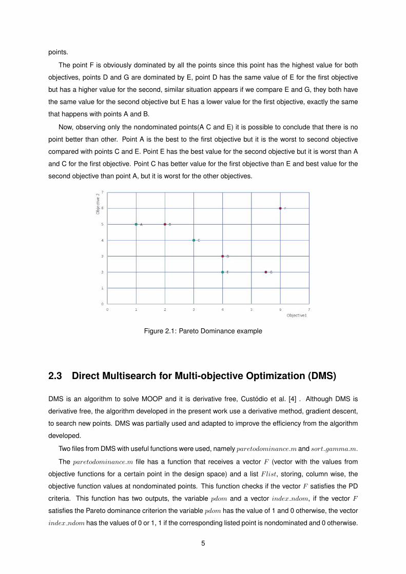
In the figure 2.1 it is possible to observe an illustrative example of the concept of PD with a group of

points in the objectives space, the goal is to minimize both objectives.

The red points (B D G and F) are the dominated points and the green points(A C E) are nondominated

4

points.

The point F is obviously dominated by all the points since this point has the highest value for both

objectives, points D and G are dominated by E, point D has the same value of E for the first objective

but has a higher value for the second, similar situation appears if we compare E and G, they both have

the same value for the second objective but E has a lower value for the first objective, exactly the same

that happens with points A and B.

Now, observing only the nondominated points(A C and E) it is possible to conclude that there is no

point better than other. Point A is the best to the first objective but it is the worst to second objective

compared with points C and E. Point E has the best value for the second objective but it is worst than A

and C for the first objective. Point C has better value for the first objective than E and best value for the

second objective than point A, but it is worst for the other objectives.

Figure 2.1: Pareto Dominance example

2.3 Direct Multisearch for Multi-objective Optimization (DMS)

DMS is an algorithm to solve MOOP and it is derivative free, Custodio et al. [4] . Although DMS is

derivative free, the algorithm developed in the present work use a derivative method, gradient descent,

to search new points. DMS was partially used and adapted to improve the efficiency from the algorithm

developed.

Two files from DMS with useful functions were used, namely paretodominance.m and sort gamma.m.

The paretodominance.m file has a function that receives a vector F (vector with the values from

objective functions for a certain point in the design space) and a list Flist, storing, column wise, the

objective function values at nondominated points. This function checks if the vector F satisfies the PD

criteria. This function has two outputs, the variable pdom and a vector index ndom, if the vector F

satisfies the Pareto dominance criterion the variable pdom has the value of 1 and 0 otherwise, the vector

index ndom has the values of 0 or 1, 1 if the corresponding listed point is nondominated and 0 otherwise.

5

Basically this function evaluates a new point, if it is nondominated the point is stored in the lists and

all the points dominated by the new one are erased from the list

The sort gamma.m file has a function that sorts a list of points according to the largest gap between

two consecutive points, in the objective domain.

This function has as input a list of points P , a list of function values corresponding to the points listed

on P , a list alfa that has the corresponding step size parameters, a variable stop alfa for the case of

existence of a stop criteria based on the step size and the value of this criteria is an input as well, called

tol stop, the last input is spread option and has values of 0, 1 or 2 according with different spread option.

As an output the function give three ordered lists, one with the points, one with the functions values

corresponding to the listed points and a list with the step size parameters also according with the list of

points.

2.4 Formulation of the Optimization Problem

A correct definition and formulation of an optimization problem it is a very important task in order to solve

the problem, and it is generally accepted that this takes about 50% of the effort to solve it, Arora [3].

If a problem is not well formulated different problems can appear, for example, if there are contradic-

tory constrains or even if there are to many constrains it is possible that the formulated problem has no

solution.

The formulation of an optimization problem generally takes four steps:

• Objectives and description of the problem

• Definition of design variables

• Optimizations criteria

• Formulation of constrains

In order to start formulating the problem first it should be done a description of the problem and

realize witch are all the requirements and objectives, it is also necessary have into account the sources

available.

The second step consists in identifying the design variables, in other words, the set of variables that

describes the problem.

This variables should be independent from each other as much as possible. If they are dependent

their values cannot be represented independently once they have constrains between them, the number

of independent variables represents the degree of freedom of the problem. This variables can have any

value that does not violate the constrains.

After identify the criteria that allow a construction of one or more mathematical functions , it is possible

to identify the variables of the problem that will give different feasible designs for the system. This

functions will give different solutions that allow to compare different designs and choose one, these

functions are called objective functions.

6

The last step consists in, identify where there is a need to do some limitations or restrictions, this

restrictions are called constrains of the problem.

All the constrains should depend on the design variables, in order to guarantee that the design is

correct. A generic mathematical formulation is given by equation 2.1.

7

8

Chapter 3

Implementation

The implementation of a computational model to solve the proposed problem for the present work is

divided in two phases.

First it is developed a model where the goal is to obtain the Pareto front for two differentiable functions

with one or two variables, using the gradient to search new points.

The second model is an adaptation of the first model to solve a topology optimization problem using

the concept of MOOP from the first developed model. Two objective functions are used, both with the

objective to minimize the compliance of the structure, for a force upwards and the other to a downwards

force. Both models are written in Matlab and they resort to derivatives to solve the problem.

3.1 Gradient Based Search Method

A gradient based search method as the name says, uses the gradient of a function to find a local mini-

mum. In order to use a method like this the function has to be continuously differentiable everywhere in

the feasible design space, where the design variables are assumed to be continuous and they can have

any value in their allowable ranges. Gradient based search methods are iterative and the calculations

performed are repeated in every iteration.

According to Arora [3] the repeated calculations in every iteration can be represent by the equation

3.1 in vector form or equation 3.2 as component form,

x(k+1) = x(k) + ∆x(k); k = 0, 1, 2, ... (3.1)

x(k+1)i = x

(k)i + ∆x

(k)i ; i = 1 to n; k = 0, 1, 2, ... (3.2)

Where,

k = superscript representing the iteration number

i = subscript denoting the design variable number

x(0) = starting point

9

∆x(k) = change in the current point

The change in the current point can written as represented in 3.3,

∆x(k) = αkd(k) (3.3)

Where d(k) is the search direction that in the present work is obtained using the value of the gradient

in the point of departure of each iteration and αk is a scalar called the step size in the search direction.

An iterative scheme using equation 3.1 and 3.2 is continued until the stop criteria is achieved. Joining

DMS and the concept of PO it is developed an algorithm to solve MOOP

3.2 Example of a MOOP algorithm

Taking as example the first presented study case:

minimize F (x) = (f(x), g(x))

f(x, y) = (1.5x− 2)2 + y2 , g(x, y) = x2 + 1.5y2

subject to − 5 ≤ x ≤ 5; −5 ≤ y ≤ 5

(3.4)

In this example the lists are initialized with the pointA(1, 1) for which the functions are worth, f(x, y) =

1.25 and g(x, y) = 2.5 and alpha = 1. The gradient of each function is calculated in equations 3.5 and

3.6. So using the gradient of f and g and applying the gradient based search method two new points

are founded and evaluated, B and C.

∇f =

dfdx

dfdy

=

2(1.5x− 2)

2y

(3.5)

∇g =

dgdx

dgdy

=

2x

3y

(3.6)

This two points are dominated by A as it is possible to observe in figure 3.1, where it is represented the

variables and objectives spaces. Once these two points are dominated they are eliminated from the lists

and it is considered unsuccessful, so the step size is divided by two and the calculations are repeated.

Now for a step size parameter of 0.5, points C and D are obtained. They are nondominated so they

are stored in the lists. If at least on of the points are stored in the lists, it is considered a success and

alpha is increased two times as is in this case.

This process is repeated until the stop criteria is reached and the expected result should be a Pareto

front, the stop criteria for this problem is the step size.

10

(a) Variables space (b) Objective space

Figure 3.1: MOOP Example

3.3 Numerical Model 1

The first numerical model developed, as it says in the beginning of this chapter, is a model where it is

possible to obtain a Pareto front for any two differentiable functions with two variables each, using the

gradient to search new points.

3.3.1 Formulation of the Problem

As is described in 2.4 the formulation of a multi-objective optimization problem generally takes four steps.

Objectives and description of the problem

The goal of this first problem is to develop a Matlab algorithm capable of find the Pareto front for any two

differentiable functions introduced by the user. These functions should be differentiable, in order to be

possible to use the gradient to find the direction of minimization of each function.

Definition of design variables

The design variables depend on the functions introduced by the user and each function have to have

one or two variables, the Matlab code is ready to receive two variables x and y.

Optimizations criteria

Since this model is capable to solve different MOOP, the optimization criteria is minimize any two func-

tions introduced by the user of the program, that depend on the design variables.

Formulation of constrains

The only constrains used in this problem are the design space of each design variable, these values are

also introduced by the user putting the lowest and the highest value that each variable can assume.

11

This problem have the fowling mathematical formulation:

minimize F (x) = (f1(x), f2(x))

subject to xL1 ≤ x1 ≤ xU1 ; xL2 ≤ x2 ≤ xU2(3.7)

where xL and xU are the lower and upper bounds respectively.

3.3.2 Description of the Model 1

The main code is in the file paretos.m and this file is composed by a call function called pareto. This

function has as input the two objective functions depending on one or two variables, the lower and upper

bounds of each design variable is also an input.

To start with, the program converts the expression of each objective function introduced in Matlab

function, in order to, make possible the calculation of the functions values and the gradient of each

function.

To initialize the search of a Pareto set of solutions it is generatedN = 500 (this value can be changed)

random points in the design domain. This initialization is more efficient than to start from only one point,

since this way we have several different points to start the search.

After the initialization, the points are evaluated one at a time in a cycle that works in the fowling way

- the values of both functions are calculated and saved in the variable Ftemp, the values of the design

variables are stored in a variable called xtemp, and the alphatemp has always the same value (one).

The variable Ftemp is an input of the function paretodominance, explained in 2.3, to evaluate the

point, the program checks if this point could belong to the set of nondominated points comparing with

all the values from Flist. In case this point is dominated, the cycle starts again analysing other point.

If the point is nondominated is inserted in the list Flist, xlist and alphalist. If there are points that are

dominated by the new point these points are eliminated from the lists.The cycle is repeated until the N

points are checked.

After this initialization, there is a set of nondominated points and the cycle that will solve the problem

will start. To start the main cycle the function sort gamma is called to find the biggest gap between

two consecutive points, in the objective space and sort the points with this criteria, as explained in 2.3.

Therefore, the first point from the list, is the point selected to start the search for new points.

The next step is to calculate the gradient of each function in the chosen point, that will give two

directions of search for two new points using expression 3.2. One uses the gradient of the first function

to obtain a new point and the second point is obtained using the gradient from the second function .

After the two new points are found, this two points are evaluated to check if they are dominated by

any existing point in the lists. If a point is nondominated is saved in the list and the existing points are

evaluated to verify if any of the old points are dominated by the new point, if there is any point dominated

by a new one, the dominated points are eliminated from the lists.

Finally, the last task from the cycle is to verify if the search for a new point was a success or not. If at

least one of the new points are added to the set of nondominated points, it is considered a success. In

12

the other hand, if any point is not added to the set of nondominated solutions it is considered a failure.

In the case of success the step size parameter is doubled and, in case of failure the step size parameter

is divided by two.

The cycle has as stop criteria, the step size parameter. When the highest value of the step size is

less than the chosen tolerance (0.0001),the stop criteria is achieved. If this criteria is never satisfied,

after a significant number of evaluations the cycle finishes and the plot of objectives functions is plotted

and therefore the problem is solved.

3.4 Numerical Model 2

The second numerical model is the one that solves the main problem proposed for this work that together

with the PD concept and the concept of topology optimization, gives an optimized structure, for two

objectives and some constrains.

Besides the functions used in the first model, this model uses two functions(topu and topd) that are

variants from the function top, this function belongs to a code of topology optimization, for more details

about this function check Sigmund [6].

3.4.1 Topology Optimization

Nowadays Topology Optimization it is a technology well established and designs obtained with these

methods are in production on a daily basis.

The optimization of the geometry and topology of structural layout has a big influence on the perfor-

mance of structures, and in the last two decades there has been a big development of this technology,

that is a very important area of structural optimization. This development is manly due to the success of

the material distribution method for generating optimal topologies of structural elements.

An efficient use of materials is important in many different areas, for example in the aerospace

and automotive industry is used to apply sizing and shape optimization to the design of structures and

mechanical elements.

The layout of a structure contains information about topology, shape and sizing of the structure and

with the material distribution method it is possible solve all three problems simultaneously.

According to Bendsoe and Sigmund [5], these three different problems address different aspects of

a structural design problem, for example, in a sizing problem the goal is typically to find the optimal

thickness distribution of a linearly elastic plate or the optimal member areas in a truss structure. The

optimal thickness distribution minimizes a physical quantity, for example, the compliance, peak stress or

deflection while equilibrium and other constraints on the state and design variables are satisfied. The

main feature of a sizing problem is that the domain of the design model and state variables is known a

priori and is fixed throughout the optimization process. In a shape optimization problem the goal is to

find the optimum shape of this domain, that is, the shape problem is defined on a domain which is now

the design variable.

13

Topology optimization of solid structures involves the determination of features such as the number

and location and shape of hole and the connectivity of the domain.

In this method, the project variables are numerical parameters that can change the material distribu-

tion in the structure with the propose of save material in regions with reduced solicitation.

There are two types of project variables, continuous or discrete. In the case of a truss, in which the

section area of the bars are used as discrete project variables, it is possible to allow that this areas can

be zero, with this there is the possibility to remove from the truss bars that has no effort, as it is possible

to see in figure 3.2 a).

Figure 3.2: Topology Optimization examples, Sigmund [6]

In figure 3.2 b) it is possible to observe an example of shape optimization.

If continuous optimization is used, as for example in a bidimensional plate, the ideal changes of

topology can be made by allowing the thickness be zero and the maximum thickness have a reasonable

value for the project. The same effect can be achieved by using the density as a project variable, where

the density can only have values between 0 and 1. An example of continuous bidimensional optimization

can be observed in figure 3.2 c).

In the present work the space design was divided in finite elements and was used, as design variable,

the relative density.

3.4.2 Solid Isotropic Material with Penalization(SIMP)

The SIMP model from Bendsøe and Sigmund [7], is an Isotropic model for solid-void interpolations in

elasticity. In SIMP a continuous variable ρ, 0 ≤ ρ ≤ 1 is introduced, resembling a density since the

volume of the structure is evaluated as

V ol =

∫Ω

ρ(x)dΩ (3.8)

In order to avoid a singular FEM problem a small lower bound is imposed, 0 < ρmin ≤ ρ, when solving

for equilibrium in full domain Ω, in this work ρmin = 0.001.

In the equilibrium analysis the relation between the material tensor Cijkl(x) and the density is given

14

by

Cijkl(ρ) = ρpC0ijkl, (3.9)

where the given material is isotropic, in other words C0ijkl is characterized by two variables, here chosen

as the Young’s modulus E0 and the Poisson ratio ν0, the interpolation 3.9 satisfies that Cijkl(0) = 0 and

Cijkl(1) = C0ijkl.

With this the final design should have density zero or one in all points, this design is a black and

white design for which the performance has been evaluated with a correct physical model.

For problems where the volume constraint is active, as in this work, Bendsøe and Sigmund [7] says

that experience shows that optimization does actually result in such designs if one chooses p sufficiently

big, typically is required that p ≥ 3. The reason is that, for such a choice, intermediate densities are

penalized; volume is proportional to stiffness, but ρ is inversely proportional.

3.4.3 Formulation of the Problem

As is described in 2.4 the formulation of a MOOP generally takes four steps.

The previous numerical model is more generic since the model can receive any differentiable func-

tion. For this problem the functions are always the same two objective functions.

Objectives and description of the problem

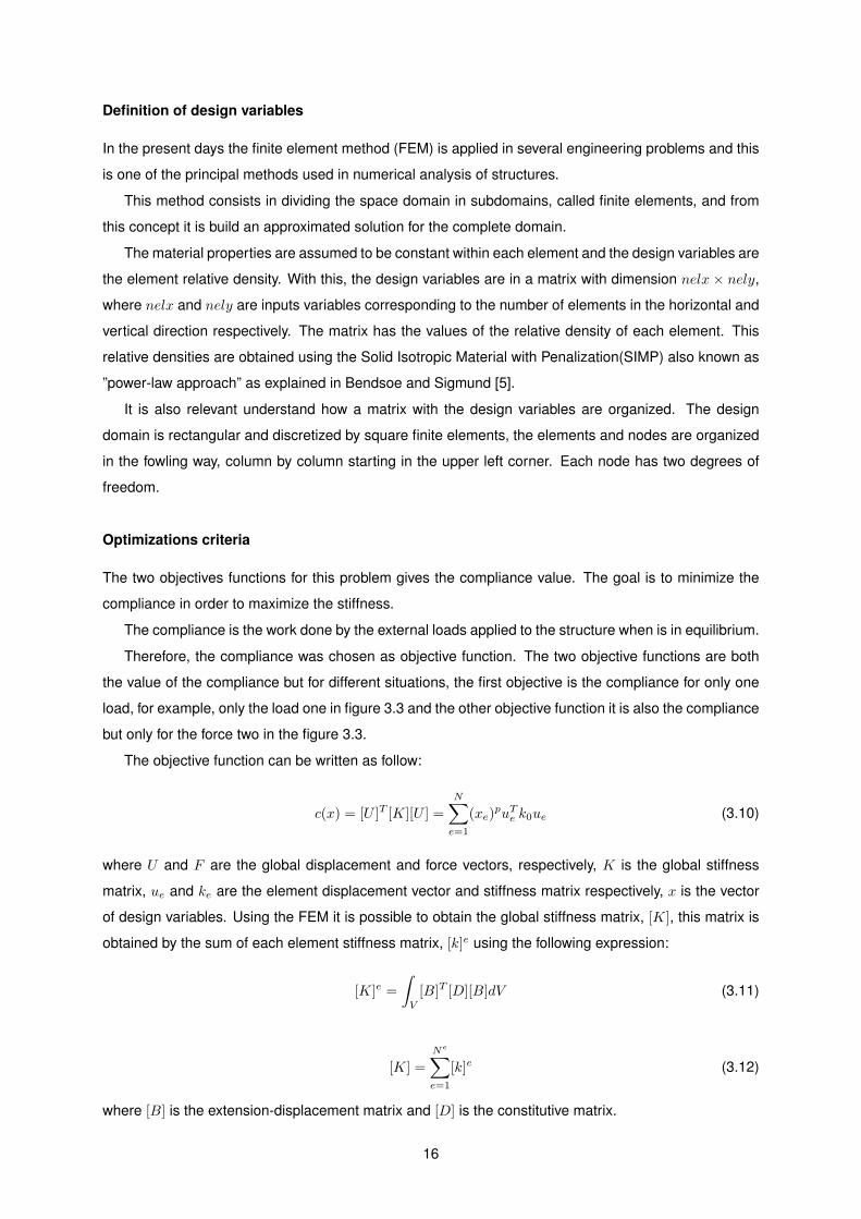
The problem treated in this model, is the TO of a bidimensional structure discretized by finite elements.

The structure is fixed at one side and subject to two loads in the tip of the opposite side, one on the

top with upwards direction and the other in the bottom downwards as it is possible to see in figure. 3.3 .

The objectives to be accomplished in this problem is the minimization of the compliance in order to

maximize the stiffness of the structures. One objective is minimization of compliance to the upwards

force case and the other is to the downwards force case.

Figure 3.3: Illustrative example of the problem Sigmund [6]

15

Definition of design variables

In the present days the finite element method (FEM) is applied in several engineering problems and this

is one of the principal methods used in numerical analysis of structures.

This method consists in dividing the space domain in subdomains, called finite elements, and from

this concept it is build an approximated solution for the complete domain.

The material properties are assumed to be constant within each element and the design variables are

the element relative density. With this, the design variables are in a matrix with dimension nelx × nely,

where nelx and nely are inputs variables corresponding to the number of elements in the horizontal and

vertical direction respectively. The matrix has the values of the relative density of each element. This

relative densities are obtained using the Solid Isotropic Material with Penalization(SIMP) also known as

”power-law approach” as explained in Bendsoe and Sigmund [5].

It is also relevant understand how a matrix with the design variables are organized. The design

domain is rectangular and discretized by square finite elements, the elements and nodes are organized

in the fowling way, column by column starting in the upper left corner. Each node has two degrees of

freedom.

Optimizations criteria

The two objectives functions for this problem gives the compliance value. The goal is to minimize the

compliance in order to maximize the stiffness.

The compliance is the work done by the external loads applied to the structure when is in equilibrium.

Therefore, the compliance was chosen as objective function. The two objective functions are both

the value of the compliance but for different situations, the first objective is the compliance for only one

load, for example, only the load one in figure 3.3 and the other objective function it is also the compliance

but only for the force two in the figure 3.3.

The objective function can be written as follow:

c(x) = [U ]T [K][U ] =

N∑e=1

(xe)puTe k0ue (3.10)

where U and F are the global displacement and force vectors, respectively, K is the global stiffness

matrix, ue and ke are the element displacement vector and stiffness matrix respectively, x is the vector

of design variables. Using the FEM it is possible to obtain the global stiffness matrix, [K], this matrix is

obtained by the sum of each element stiffness matrix, [k]e using the following expression:

[K]e =

∫V

[B]T [D][B]dV (3.11)

[K] =

Ne∑e=1

[k]e (3.12)

where [B] is the extension-displacement matrix and [D] is the constitutive matrix.

16

From the vector of loads, f , and from the stiffness matrix is possible to obtain the displacement fields,

u, using the fowling expression:

[K][U ] = f (3.13)

Knowing that the compliance is the work done by the applied loads in the structure, it is possible to relate

with the displacement fields as it follows:

c = fT [U ] = [U ]T [K][U ] (3.14)

In order obtain the gradient from the objective function, it will be written the expressions of the function

and its own gradient, in relation to the design variables, it is possible to realize that:

c(u, x) = fTu (3.15)

dc

dx(u, x) =

∂c

∂x+∂c

∂u

∂u

∂x= fT

∂u

∂x(3.16)

Looking to equation 3.15 it is possible to notice that the objective function does not explicitly depend on

the design variables, so the partial derivative ∂c∂x is null. Although there is not an explicit relation between

the objective function or the gradient function with the design variables, it is still possible to easily obtain

the gradient function, using the displacement fields 3.14.

The gradient can be computed using the adjoint method, according with Christensen and Klarbring

[8] as;dc

dx= −[U ]T

∂[K]

∂x[U ] (3.17)

Following the Bendsoe [9] and Sigmund [6] a heuristic updating scheme for the design variables can

be formulated as

xnewe =

max(xmin, xe −m)

if xeBηe ≤ max(xmin, xe −m),

xeBηe

if max(xmin, xe −m) < xeBηe < min(1, xe +m),

min(1, xe +m)

if min(1, xe +m) ≤ xeBηe ,

(3.18)

where m (move) is a positive move limit, η(=1/2) is a numerical damping coefficient and Be is found from

the optimality conditions as

Be =− ∂c∂xe

λ ∂V∂xe

, (3.19)

where λ is a Lagrangian multiplier that can be found by a bi-sectioning algorithm in order to satisfy a

volume constraint, so the volume constrain is already implicit in the algorithm of TO.

17

The sensitivity of the objective function is found as

∂c

∂xe= −p(xe)p−1uTe k0ue (3.20)

Formulations of constrains

For the resolution of this topology optimization problem there are three constrains,

V (x)V0

= f

KU = F

0 < xmin ≤ x ≤ 1

(3.21)

The first two are equality constrains V (x) and V0 is the material material volume and design domain

volume respectively and f is the prescribed volume fraction. U and F are the global displacement and

the force vectors, respectively, K is the global stiffness matrix.

The last one is an inequality constrain, where x is the vector of design variables and xmin is a vector

of minimum relative densities(non zero to avoid singularity).

This problem have the fowling mathematical formulation:

minimize F (x) = (f1(x), f2(x))

f1(x) = c1(x) = [U ]T [K][U ] , f2(x) = c2(x) = [U ]T [K][U ]

subject toV (x)

V0= f

KU = F

0 < xmin ≤ x ≤ 1

(3.22)

3.4.4 Description of the Model 2

As it is said in the beginning of this chapter, the second model is an adaptation from the first model.

There are some parts of the algorithm that are similar but significant changes were performed and more

functions are used. The main code is in the file twoloads.m.

To initialize the problem there are three options.

The first option initializes the program putting in each element of the design domain (matrix nelx ×

nely) with the value of the volume fraction, this is the departure point to search for a set of nondominated

points.

In the second option it is possible to load a set of points and verifies which are dominated points and

eliminates them.

The third option of initialization is similar to the second option. In this option three points are carefully

chosen. This three points are taken from a single objective problem. Two points where only one load

18

is applied and one point with the load from objective one and two, notice that the third point is also a

singular objective function where the two loads are applied.

In all options the values of the objective functions for the points are computed and saved in a list

called Flist, the design variables are in the list xlist and finally, are created a list with the step size

called alphalist.

After the initialization of the lists the main cycle starts. Fist of all two functions are called, topu and

topd. These function have six inputs, nelx and nely are the number of finite elements in the horizontal

and vertical direction respectively, volfrac is the volume fraction, penal is the penalization used in the

SIMP method, rmin is the filter size divided by the element size and x is the point where the search

departs to find a new point.

The output of these functions are the compliance value for the point x and the next point founded,

so the objective functions are calculated in this functions. topu is for the objective 1 and topd is for

the objective 2, both objectives are represented in figure 3.3. When these two functions are called it is

obtained the compliance values for the two objectives and two new points x1 and x2, the new points are

always with the same step size value, so in order to vary the step size it is done a calculation to reduce

or increase the step size using the fowling expression:

xnew = (xnew′ − xi)× alphalist(i) + xi (3.23)

, where xi is the point of departure, alphalist(i) is the corresponding coefficient of step size parameter

that can have positive values less or equal to 1, xnew′ is the point given by the objective function and

xnew is the new point founded using the step size parameter.

After having two new points, these points need to be checked, in order to realize if they are dominated

or nondominated. To do this there is the necessity to call again the function topu and topd for each point,

to know which are the values of the compliances for this point. Notice that in this case the new points

obtained by the functions are not used, so there is a computational waste since there are some calculus

done in the function that are not used.

With the values for the compliance the points are evaluated the same way as in the previous model.

These values for a point are stored in a vector called Ftemp and using the function paretodominance

the point is compared with the points stored in Flist. If the point is dominated by any of the points it is

discarded, if it is nondominated is added to Flist and all the points from Flist are checked to see if any

point is dominated by the new point, in this case the dominated points are discarded.

In order to increase the performance of the algorithm, when a point is successful added to our set of

nondominated solutions, a symmetric point is added turning upside down the columns of the matrix x.

Basically what happens when the columns are turned up side down, is that the material in the ele-

ments will change position to the symmetric position in relation to the blue line in figure 3.4.

Since the functions for both objectives are the same, what happens is that when a point is added to

the set of nondominated solutions, by performing the change in the columns a new point appears. This

new point in the space of objectives will be symmetric in relation to the bisectrix of the odd quadrants

19

Figure 3.4: Illustrative Example

and the structure obtained is symmetric as it is possible to observe in figure 3.5, this simple method

makes the algorithm more efficient.

(a) Found point (b) Symmetric point

Figure 3.5: Illustrative Example

After the find two new points and evaluate them, the step size parameter is changed in case of

success it is increased two times otherwise it is decreased by half. To be considered a success at least

one of the two points need to be a nondominated solution.

Finally the last procedure done in the cycle is to choose the next point of departure, using the function

sort gamma that searches for the largest gap between two consecutive points and sorts the lists.

20

Chapter 4

Results

In this chapter, the obtained results in this work are presented fowling the natural sequence of work.

First the results of the first model are presented and then for the second model developed. In each

model the results are presented fowling a criteria of complexity, starting from the simplest to the most

complex case.

Both models aim to optimize two objective functions. The first model search the optimal Pareto set for

two differentiable functions. While the second model also search for a optimal Pareto set of solutions to

minimize the compliance, maximizing the stiffness for a bidimensional structure subject to two different

objectives,these objective functions are the compliance for two different applied forces.

4.1 Problem Description and Results for Model 1

The first model gives a set of nondominated points for a MOOP, in the first examples tested the program

was simpler, with the increase of complexity in the following tested function emerged the necessity to

improve the efficiency of the code, since the code was taking too long to solve the problem.

The stop criteria for this solution is the maximum value in the step size parameter list, called alphalist,

that should be bigger than the tolerance(tolerance=0.001) or if the function is evaluated 1000 times. If

one of these criteria are achieved the program stops and plot the graph of the set of nondominated

solutions.

If the solution is not satisfactory it is possible to increase the number of evaluation in order to improve

the results.

4.1.1 Case 1

Find the optimal Pareto set of solution for the fowling problem:

minimize F (x) = (f(x), g(x))

f(x, y) = (1.5x− 2)2 + y2 , g(x, y) = x2 + 1.5y2

subject to − 5 ≤ x ≤ 5; −5 ≤ y ≤ 5

(4.1)

21

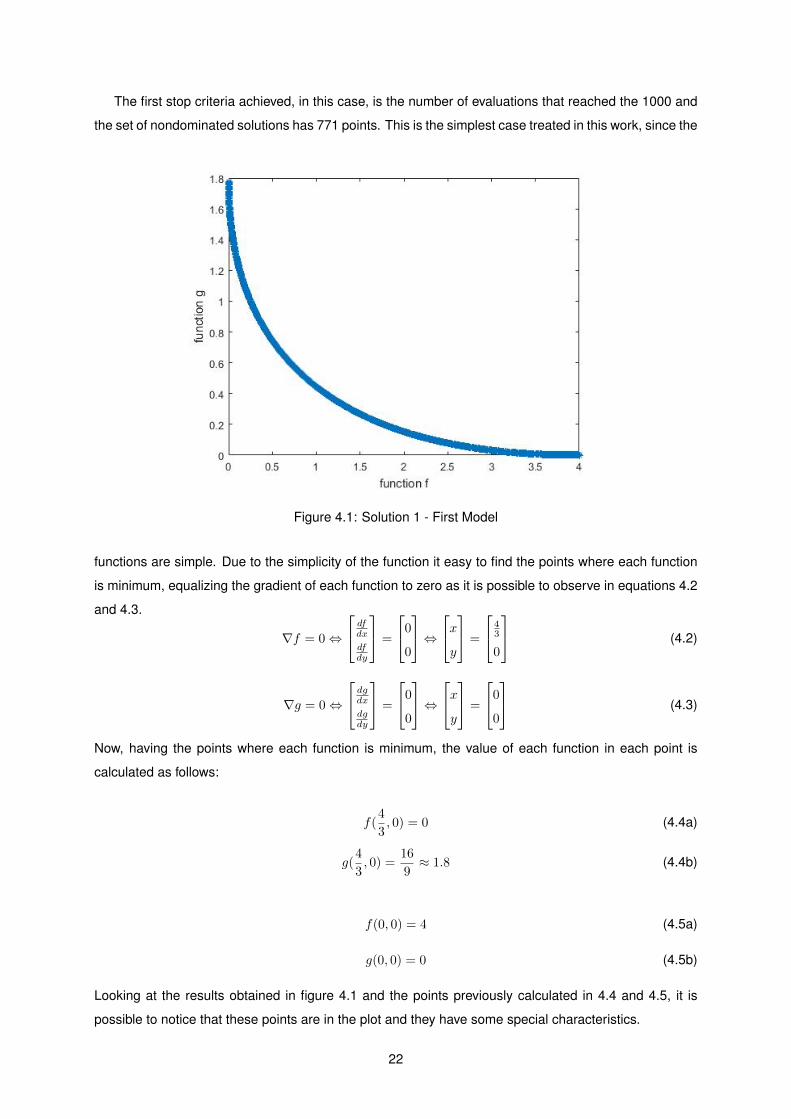
The first stop criteria achieved, in this case, is the number of evaluations that reached the 1000 and

the set of nondominated solutions has 771 points. This is the simplest case treated in this work, since the

Figure 4.1: Solution 1 - First Model

functions are simple. Due to the simplicity of the function it easy to find the points where each function

is minimum, equalizing the gradient of each function to zero as it is possible to observe in equations 4.2

and 4.3.

∇f = 0⇔

dfdx

dfdy

=

0

0

⇔xy

=

43

0

(4.2)

∇g = 0⇔

dgdx

dgdy

=

0

0

⇔xy

=

0

0

(4.3)

Now, having the points where each function is minimum, the value of each function in each point is

calculated as follows:

f(4

3, 0) = 0 (4.4a)

g(4

3, 0) =

16

9≈ 1.8 (4.4b)

f(0, 0) = 4 (4.5a)

g(0, 0) = 0 (4.5b)

Looking at the results obtained in figure 4.1 and the points previously calculated in 4.4 and 4.5, it is

possible to notice that these points are in the plot and they have some special characteristics.

22

The point obtained from the gradient of the function f is where the function f has the lowest value

and where g is maximum, the same happens with the point obtained from the gradient of g, is where g

is minimum and f is maximum, as expected.

That the point obtained, for example from the equation 4.2, is the minimum for the function f it

was already known, but the fact that this exact point is also the maximum value for g, in the set of

nondominated solutions, it was not expected at first. I

If we take into account the PD concept this makes sense, since in a set of nondominated points there

is not a point that we can say that is better than other, when comparing two points if the first point is

better for one objective is worst for the other, so the point where one of the objectives is minimum it is

expected that the other objective is maximum.

4.1.2 Case 2

Find the optimal Pareto set of solutions for the fowling problem:

minimize F (x) = (f(x), g(x))

f(x, y) = x , g(x, y) = 1 + y2 − x− a sin(bπx)

subject to 0 ≤ x ≤ 1; −2 ≤ y ≤ 2

(4.6)

This multi-objective optimization problem is an example present in Deb [1], this function has some

curious solutions if you slightly change the parameters a and b, it is possible to obtain a convex and a

non convex Pareto front.

(a) Solution 1 (b) Solution 2

Figure 4.2: Case 2 - Expected solution from Deb [1]

Since this function can give such different solutions, it is an interesting test to verify if the program is

working correctly, with the available data about this problem is possible compare the solutions obtained

by the program developed for this work with the analytical solution.

The two cases studied have the fowling values for the parameters a and b, the first problem is where

23

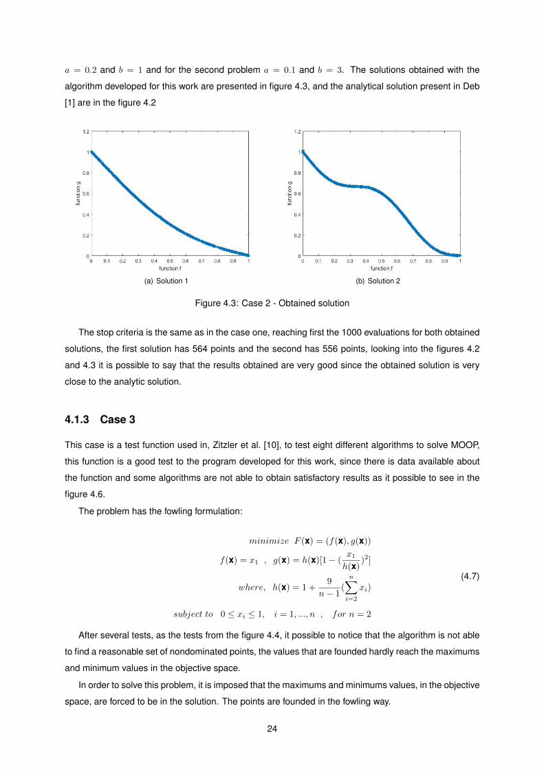
a = 0.2 and b = 1 and for the second problem a = 0.1 and b = 3. The solutions obtained with the

algorithm developed for this work are presented in figure 4.3, and the analytical solution present in Deb

[1] are in the figure 4.2

(a) Solution 1 (b) Solution 2

Figure 4.3: Case 2 - Obtained solution

The stop criteria is the same as in the case one, reaching first the 1000 evaluations for both obtained

solutions, the first solution has 564 points and the second has 556 points, looking into the figures 4.2

and 4.3 it is possible to say that the results obtained are very good since the obtained solution is very

close to the analytic solution.

4.1.3 Case 3

This case is a test function used in, Zitzler et al. [10], to test eight different algorithms to solve MOOP,

this function is a good test to the program developed for this work, since there is data available about

the function and some algorithms are not able to obtain satisfactory results as it possible to see in the

figure 4.6.

The problem has the fowling formulation:

minimize F (x) = (f(x), g(x))

f(x) = x1 , g(x) = h(x)[1− (x1

h(x))2]

where, h(x) = 1 +9

n− 1(

n∑i=2

xi)

subject to 0 ≤ xi ≤ 1, i = 1, ..., n , for n = 2

(4.7)

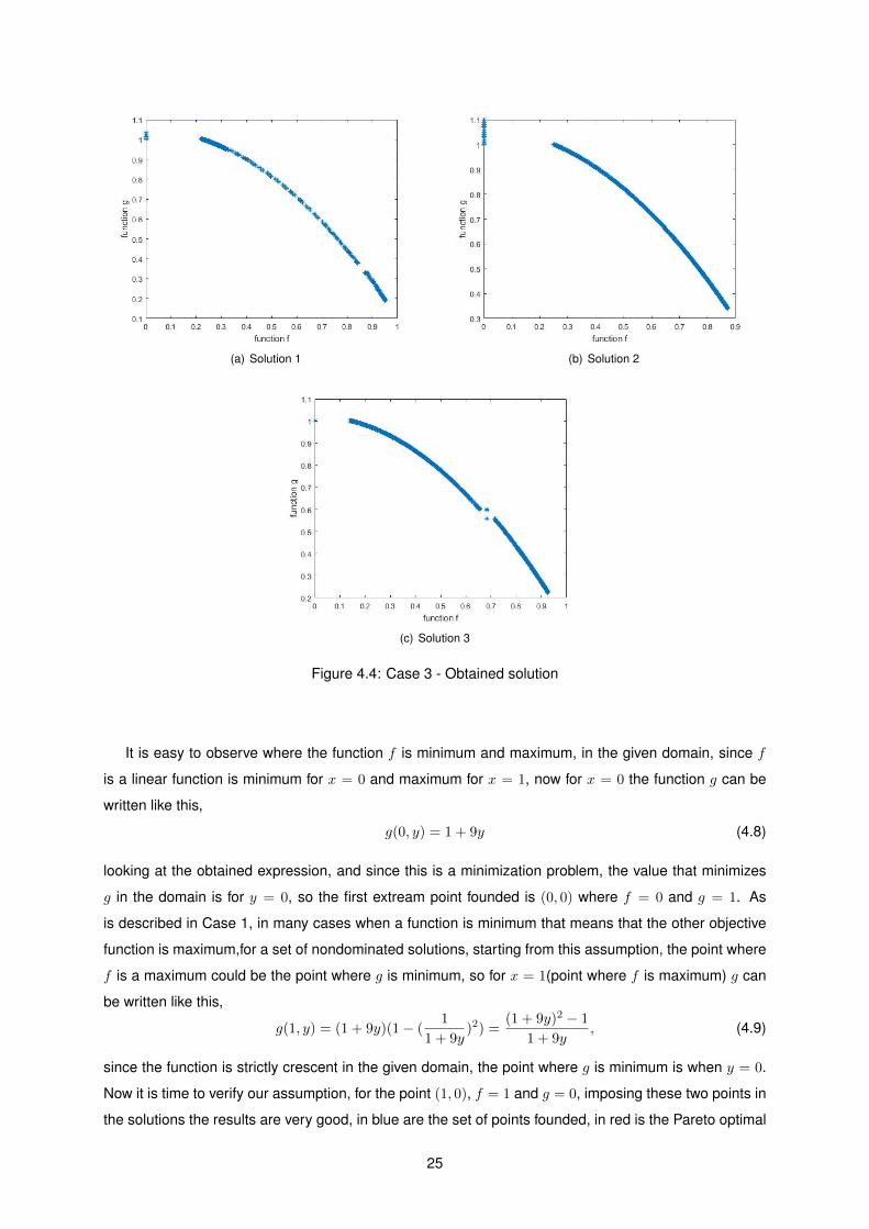
After several tests, as the tests from the figure 4.4, it possible to notice that the algorithm is not able

to find a reasonable set of nondominated points, the values that are founded hardly reach the maximums

and minimum values in the objective space.

In order to solve this problem, it is imposed that the maximums and minimums values, in the objective

space, are forced to be in the solution. The points are founded in the fowling way.

24

(a) Solution 1 (b) Solution 2

(c) Solution 3

Figure 4.4: Case 3 - Obtained solution

It is easy to observe where the function f is minimum and maximum, in the given domain, since f

is a linear function is minimum for x = 0 and maximum for x = 1, now for x = 0 the function g can be

written like this,

g(0, y) = 1 + 9y (4.8)

looking at the obtained expression, and since this is a minimization problem, the value that minimizes

g in the domain is for y = 0, so the first extream point founded is (0, 0) where f = 0 and g = 1. As

is described in Case 1, in many cases when a function is minimum that means that the other objective

function is maximum,for a set of nondominated solutions, starting from this assumption, the point where

f is a maximum could be the point where g is minimum, so for x = 1(point where f is maximum) g can

be written like this,

g(1, y) = (1 + 9y)(1− (1

1 + 9y)2) =

(1 + 9y)2 − 1

1 + 9y, (4.9)

since the function is strictly crescent in the given domain, the point where g is minimum is when y = 0.

Now it is time to verify our assumption, for the point (1, 0), f = 1 and g = 0, imposing these two points in

the solutions the results are very good, in blue are the set of points founded, in red is the Pareto optimal

25

front given by the analytical expression,

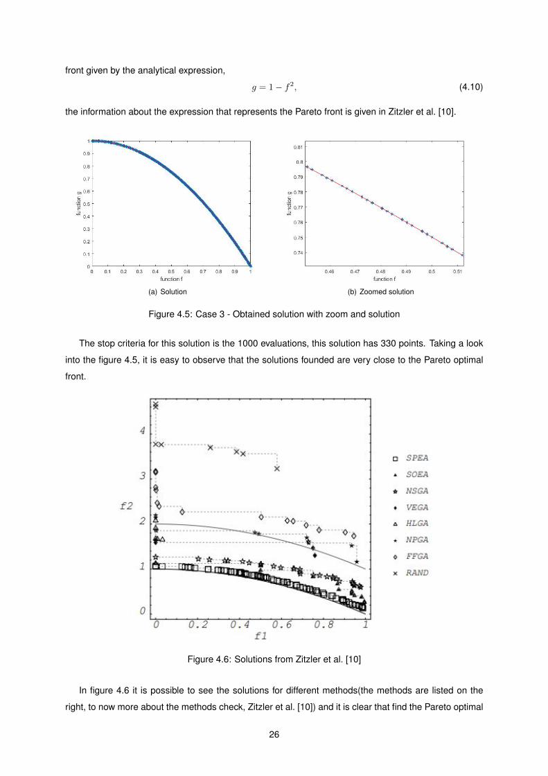
g = 1− f2, (4.10)

the information about the expression that represents the Pareto front is given in Zitzler et al. [10].

(a) Solution (b) Zoomed solution

Figure 4.5: Case 3 - Obtained solution with zoom and solution

The stop criteria for this solution is the 1000 evaluations, this solution has 330 points. Taking a look

into the figure 4.5, it is easy to observe that the solutions founded are very close to the Pareto optimal

front.

Figure 4.6: Solutions from Zitzler et al. [10]

In figure 4.6 it is possible to see the solutions for different methods(the methods are listed on the

right, to now more about the methods check, Zitzler et al. [10]) and it is clear that find the Pareto optimal

26

set for these functions it is not easy.

4.1.4 Case 4

This case is also a test function used in Zitzler et al. [10], to test eight different algorithms to solve the

MOOP, again this function is a good test to the program developed, because as the previous case there

is data available about this function and some tested algorithms by [10] were not able to find satisfactory

solutions, and the aspect of the expected solution is very different from all the cases shown in this work.

The problem has the fowling formulation:

minimize F (x) = (f(x), g(x))

f(x) = x1 , g(x) = h(x)[1−√

x1

h(x)− x1

h(x)sin(10πx1)]

where, h(x) = 1 +9

n− 1(

n∑i=2

xi)

subject to 0 ≤ xi ≤ 1, i = 1, ..., n , for n = 2

(4.11)

The results founded are present in, figure 4.7, the stop criteria for this solution is the number of

evaluations and this solution has 409 points.

Figure 4.7: Solution for case 4

Since there is useful data, the optimal Pareto front analytical expression from figure 4.7, lets compare

that information with the obtained solution. The expected optimal Pareto front analytical expression is

27

the fowling:

g = 1−√f − f sin(10πf)

where,

f =

[0, 0.0830015349] ∪ [0.1822287280, 0.2577623634] ∪ [0.4093136748, 0.4538821041]

∪[0.6183967944, 0.6525117038] ∪ [0.8233317983, 0.8518328654]

(4.12)

Comparing the expected solution and the computed solution it is possible to say that the same

problem that appeared in case 3 are present here. The algorithm has difficulty reaching the tips of the

lines where the Pareto optimal set of solutions is.

This problem can lead to some results far from the Pareto optimal set, looking into the figure 4.8 b)

it is possible to notice that the solution obtained does not reach the tip of the line on the left side, that

allows several points to be in the nondominated solution that should not be there, as it is possible to

observe on the black circle in the figure 4.8 b).

(a) Solution vs expected solution (b) Zoomed solutions

Figure 4.8: Case 4 - Obtained solution with the expected solution and zoom

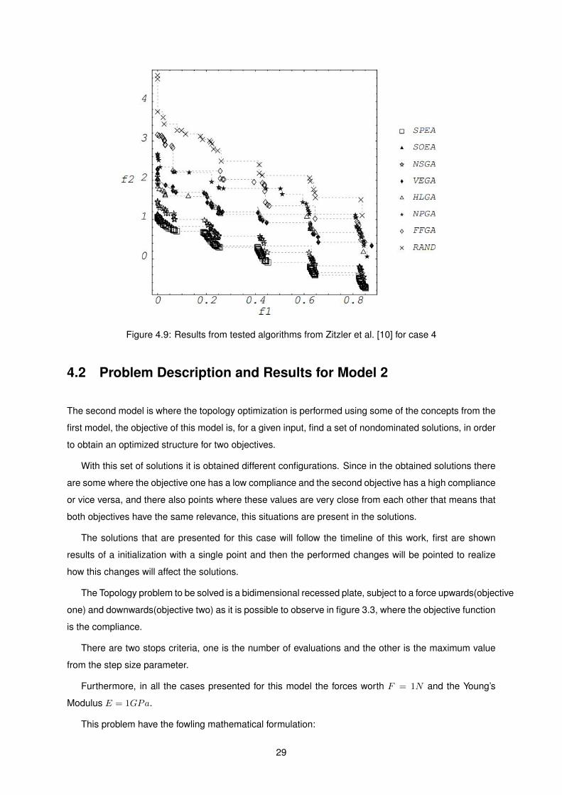
In figure 4.9 are presented the solutions from Zitzler et al. [10], obtained using different algorithms.

Although the identified problems, the solution obtained from the algorithm developed in this work is better

than the most of the solutions in figure 4.9 and it is close to the Pareto optimal set.

28

Figure 4.9: Results from tested algorithms from Zitzler et al. [10] for case 4

4.2 Problem Description and Results for Model 2

The second model is where the topology optimization is performed using some of the concepts from the

first model, the objective of this model is, for a given input, find a set of nondominated solutions, in order

to obtain an optimized structure for two objectives.

With this set of solutions it is obtained different configurations. Since in the obtained solutions there

are some where the objective one has a low compliance and the second objective has a high compliance

or vice versa, and there also points where these values are very close from each other that means that

both objectives have the same relevance, this situations are present in the solutions.

The solutions that are presented for this case will follow the timeline of this work, first are shown

results of a initialization with a single point and then the performed changes will be pointed to realize

how this changes will affect the solutions.

The Topology problem to be solved is a bidimensional recessed plate, subject to a force upwards(objective

one) and downwards(objective two) as it is possible to observe in figure 3.3, where the objective function

is the compliance.

There are two stops criteria, one is the number of evaluations and the other is the maximum value

from the step size parameter.

Furthermore, in all the cases presented for this model the forces worth F = 1N and the Young’s

Modulus E = 1GPa.

This problem have the fowling mathematical formulation:

29

minimize F (x) = (f(x), g(x))

f(x) = c1(x) = [U ]T [K][U ] , g(x) = c2(x) = [U ]T [K][U ]

subject toV (x)

V0= f

[K][U ] = [F ]

0 < xmin ≤ x ≤ 1

(4.13)

4.2.1 Case 1

The first present case intends to perceive how the penalization affects the result, to do this, three tests

testes are preformed with a mesh of 30 by 30 elements, volume fraction of 0.4, filter size of 1.2, the

same initialization,all the elements equal to the volume fraction, and a change in the penalization for

each test.

Figure 4.10: Pareto front behaviour with change in penalty

In figure 4.11 are represented the nondominated set of solutions, in the objective space, found for

the three performed tests , where p is the penalty used, in table 4.1 are the number of points found for

30000 evaluations each.

With the change of penalty it is possible to observe that the Pareto curve moves, then the higher the

penalty the greater the compliance. Now observing the obtained structures for each test in figure 4.11,

the increase in penalties have the expected effect on the structure, reduce the grey dots.

Gray dots are undesirable because they have intermediate densities, for this reason there are more

30

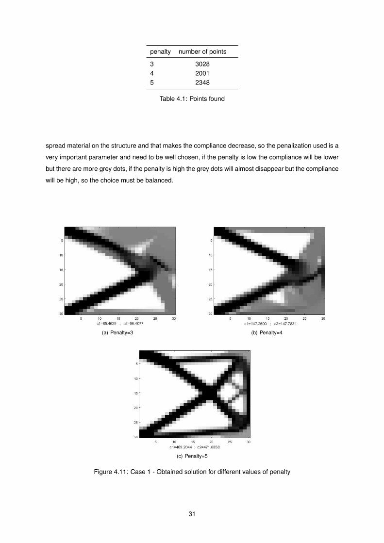
penalty number of points

3 30284 20015 2348

Table 4.1: Points found

spread material on the structure and that makes the compliance decrease, so the penalization used is a

very important parameter and need to be well chosen, if the penalty is low the compliance will be lower

but there are more grey dots, if the penalty is high the grey dots will almost disappear but the compliance

will be high, so the choice must be balanced.

(a) Penalty=3 (b) Penalty=4

(c) Penalty=5

Figure 4.11: Case 1 - Obtained solution for different values of penalty

31

4.2.2 Case 2

In this case the solutions is obtained for a mesh of 20 by 30 elements, as it is possible to observe in figure

4.12, the penalty is equal to 3.5, the size of the filter is 1.5 and the stop criteria is 15000 evaluations.

(a) c1≈c2 (b) c1 >> c2

(c) c1 << c2 (d) Location of chosen points in front of Pareto

Figure 4.12: Case 2 - Obtained solutions

The solution obtained in this case is unexpected because it is different from all the other obtained

solutions during the tests, once all the other obtained solutions when two points where c1 >> c2 and

the other point c1 << c2 are chosen, the obtained solutions are almost symmetric. It is relevant to point

that the part of the algorithm that saves a symmetric point when a successful point is found was not

implemented when this solution was obtained otherwise this solution would not be possible.

Despite the solution at first glance may make you think there is something wrong, the explanation for

this solution is simple, the obtained structure is similar to the scheme in figure 4.13 and what happens is

that the force two is transmitted to the node where the force one is applied, basically behaves like a hang-

ing bar, that is why point a), b) and c) despite different values for the compliance the obtained solutions

are similar.

32

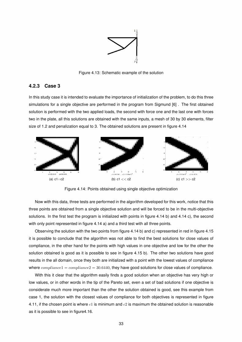
Figure 4.13: Schematic example of the solution

4.2.3 Case 3

In this study case it is intended to evaluate the importance of initialization of the problem, to do this three

simulations for a single objective are performed in the program from Sigmund [6] . The first obtained

solution is performed with the two applied loads, the second with force one and the last one with forces

two in the plate, all this solutions are obtained with the same inputs, a mesh of 30 by 30 elements, filter

size of 1.2 and penalization equal to 3. The obtained solutions are present in figure 4.14

(a) c1=c2 (b) c1 << c2 (c) c1 >> c2

Figure 4.14: Points obtained using single objective optimization

Now with this data, three tests are performed in the algorithm developed for this work, notice that this

three points are obtained from a single objective solution and will be forced to be in the multi-objective

solutions. In the first test the program is initialized with points in figure 4.14 b) and 4.14 c), the second

with only point represented in figure 4.14 a) and a third test with all three points.

Observing the solution with the two points from figure 4.14 b) and c) represented in red in figure 4.15

it is possible to conclude that the algorithm was not able to find the best solutions for close values of

compliance, in the other hand for the points with high values in one objective and low for the other the

solution obtained is good as it is possible to see in figure 4.15 b). The other two solutions have good

results in the all domain, once they both are initialized with a point with the lowest values of compliance

where compliance1 = compliance2 = 30.6440, they have good solutions for close values of compliance.

With this it clear that the algorithm easily finds a good solution when an objective has very high or

low values, or in other words in the tip of the Pareto set, even a set of bad solutions if one objective is

considerate much more important than the other the solution obtained is good, see this example from

case 1, the solution with the closest values of compliance for both objectives is represented in figure

4.11, if the chosen point is where c1 is minimum and c2 is maximum the obtained solution is reasonable

as it is possible to see in figure4.16.

33

(a) Nondominated solutions zoomed in low values of compli-ance

(b) Nondominated solutions zoomed in high values of compli-ance

Figure 4.15: Solutions obtained from three different initializations

Figure 4.16: Point from the tip of the Pareto front

Once again it is possible to conclude that the initialization of the algorithm is very important as it was

in the first model.

In figure 4.17 it is possible to observe how the structure configurations change along the Pareto front,

in image b) is one of the points used in the initialization where objective one is minimum but objective two

is maximum. Starting from a point where the compliances have similar values ,image c), and then chose

some points along one direction of the Y axe it is possible to observe how the structure is changing, the

points in the other direction are not represented once they are symmetric to these points.

34

(a) Objective Space (b) Initial point from figure 4.14b) (c) c1=30.2 andc2=34.19

(d) c1=28.64 c2=115.2 (e) c1=28.15 c2=207.2 (f) c1=27.86 c2=303.8

Figure 4.17: Evolution of the structure along the Pareto Front

35

36

Chapter 5

Conclusions

This chapter aims at exposing the conclusions drawn from the work developed in this thesis.

These are presented in a more global context, serving as a reflection on the whole process built

around the central question that defines the problem of multi-objective and topological optimization.

Based on the results presented in the previous chapter, it can be stated that the initial objective

proposed was successfully fulfilled. Build two computational models.

The first one was developed to determine the optimal Pareto front from two differentiable functions

using derivative methods and the second model was developed to determine an optimized structure to

two different objectives using the concepts from the first model to also find the optimal Pareto front for

two different objective functions.

5.1 Achievements

The results from the first developed model are very good since the obtained solutions match with ex-

pected solutions and were solved very fast. With exception of the last case that the results are slightly

different from the expected solutions but still good.

This results can be improved if the only stop criteria were the step size parameter but would take

more time to obtain the solution.

In case 3 and 4 there are data available from eight different algorithms tested by Zitzler et al. [10],

and comparing this solutions with the computed solution it is clear that the computed solution is better

than almost every solution from Zitzler et al. [10], with exception from one tested method that the results

are practically the same as the computed in this work.

In the second model the results were not so good as the ones from the first model.

This could be because of having a bigger objective domain, notice that the objective functions has

values of an order of magnitude from 10 to 108, while in the first models that magnitude were between

0 and 10. So to find a set of solutions in all the domain will require more evaluations of the objective

function being made to obtain a solution in the whole domain for this model.

37

Another detail that makes this algorithm slower is that for a 30 by 30 mesh a point has 900 coordi-

nates, whereas in the first algorithm a point has only two coordinates.

Finally what slows down this algorithm even more is the analysis of finite elements that has to solve

many equations in every iteration.

For a topology problem it is important to choose well the all parameters. This decision should be

done by a decision maker with enough experience, for example, it is expected that the solution obtained

does not have gray dots. To this there is a need to change a penalization to a bigger value but if it is to

high the compliance will be high as well so this is a balanced choice that will require a decision maker

with experience in the field.

From the results of both models it is possible to conclude that a good initialization is very important

to obtain good results. Again, a decision maker with experience in the field is important to choose where

the algorithm will be initialized and what changes should be done, in order to, obtain a satisfactory result,

this makes the process of optimizations an iterative process.

Another interesting conclusion reached during the development of this thesis is that this technology

can give us an unconventional solution, as the solution from 4.2.2.

5.2 Future Work

Having into account the developed programs and the obtained results in this thesis, some proposals for

future work are presented here:

• Can be develop a tool that forces some points to be zero or one. This will be helpful if the technol-

ogy is used by a decision maker with relevant experience, for example with the obtained solutions

in figure 4.11 c), as it is possible to see in figure 5.1 inside the blue circle, there are some grey

dots and the black dots are in contact only in the node and, this is not a good configuration. Prob-

ably that area does not need to have material, with this tool a decision maker with experience

can force that area to be white helping the algorithm to find a better solution and less expensive

computationally, since those points will have always the same value.

Figure 5.1: Illustractive example from the solution obtained in figure 4.11

38

• Improve the efficiency of the algorithm in order to achieve the step size stop criteria

• Adapt the algorithm to solve more than two objectives

39

40

Bibliography

[1] K. Deb. Multi-Objective Optimization Using Evolutionary Algorithms. John Wiley & Sons, Inc., New

York, NY, USA, 2001. ISBN 047187339X.

[2] K. Miettinen. Nonlinear Multiobjective Optimization, volume 12 of International Series in Operations

Research & Management Science. Kluwer Academic Publishers, Boston, USA, 1999.

[3] J. S. Arora. Introduction to Optimum Design. Academic Press is an imprint of Elsevie, 3rd edition,

2011. ISBN:978-0128102831.

[4] A. L. Custodio, J. F. A. Madeira, A. I. F. Vaz, and L. N. Vicente. Direct multisearch for multiobjective

optimization. SIAM Journal on Optimization, 21(3):1109–1140, 2011. doi: 10.1137/10079731X.

URL https://doi.org/10.1137/10079731X.

[5] M. P. Bendsoe and O. Sigmund. Topology Optimization: Theory, Methods and Applications.

Springer, Feb. 2004. ISBN 9783540429920.

[6] O. Sigmund. A 99 line topology optimization code written in matlab. Springer-Verlag, 2001.

[7] M. P. Bendsøe and O. Sigmund. Material interpolation schemes in topology optimization. Archive

of Applied Mechanics, 69(9):635–654, Nov 1999. ISSN 1432-0681. doi: 10.1007/s004190050248.

URL https://doi.org/10.1007/s004190050248.

[8] P. W. Christensen and A. Klarbring. An Introduction to Structural Optimization. Solid Mechanics

and Its Applications. ISBN 978-1-4020-8665-6. doi: 10.1007/978-1-4020-8666-3.

[9] M. P. Bendsoe. Optimization of Structural Topology, Shape, and Material.

[10] E. Zitzler, K. Deb, and L. Thiele. Comparison of Multiobjective Evolutionary Algorithms: Empirical

Results. Evolutionary Computation, 8(2):173–195, 2000.

41

42