Multi-period aerobic groundwater bioremediation system design; ACO...

Scientia Iranica A (2014) 21(3), 469{479

Sharif University of TechnologyScientia Iranica

Transactions A: Civil Engineeringwww.scientiairanica.com

Multi-period aerobic groundwater bioremediationsystem design; ACO approach

M. Saeedi, A. Afshar and H. Hosseinzadeh�

Department of Civil Engineering, Iran University of Science and Technology, Tehran, P.O. Box 16765-163, I.R. Iran.

Received 12 May 2012; received in revised form 28 September 2013; accepted 4 November 2013

KEYWORDSGroundwater;Contamination;Bioremediation;Optimization;Ant colony;Dynamic pumping.

Abstract. The optimal groundwater bioremediation design problem is complex, nonlin-ear, and computationally expensive. In this paper, an improved Ant Colony Optimization(ACO) algorithm is employed for optimizing a groundwater bioremediation problem, andthe BIOPLUMEII model is used to simulate aquifer hydraulics and the bioremediationprocess. Injection and extraction pumping rates and well locations are treated as decisionvariables. Optimization results show that the proposed approach performs better thanthe Genetic Algorithm (GA), Simulated Annealing (SA) and the hybrid SA-GA algorithm,called Parallel Recombinative Simulated Annealing (PRSA), and reduces the computationaltime of a number of function evaluations compared with the mentioned algorithms.Applying the optimal dynamic pumping strategy in the second stage reduces bioremediationcosts by 13:3%.c 2014 Sharif University of Technology. All rights reserved.

1. Introduction

A variety of technologies have been examined for restor-ing the quality of contaminated groundwater to achieveremedial measures such as allowed concentration ofcontaminant. It is usually costly to implement aremediation program due to slow contaminant-removalrates and complex hydrogeological and biochemicalconditions. Therefore, �nding cost e�ective ways forremediation programs is important. To improve reme-diation design, application of simulation-optimizationmethods has become an area of active research [1]. Pre-vious studies have successfully developed optimizationtechniques to solve groundwater remediation designproblems.

Examples of such optimization techniques applied

*. Corresponding author. Tel.: +98 912 7069072;Fax: +98 21 77240398E-mail addresses: [email protected] (M. Saeedi);a [email protected] (A. Afshar); [email protected](H. Hosseinzadeh)

to groundwater remediation design include linear pro-gramming [2], nonlinear programming [3], dynamicprogramming [4], simulated annealing [5], and GeneticAlgorithms (GA) [6].

The solution of this complex and nonlinear prob-lem is computationally intensive [7]. Di�erent analyti-cal and heuristic alternatives for a solution have beenproposed to solve this problem. Heuristic methodseliminate the requirement of computing derivatives,with respect to decision variables, and are also easilycoupled with simulators. One heuristic technique is theant colony algorithm. The Ant Colony Optimization(ACO) method applied to combinatorial optimizationproblems was originally developed by Dorigo [8]. Theformulation of this algorithm is straightforward, withno requirement for computing derivatives. The antcolony is one optimization method not applied togroundwater remediation problems.

It is the purpose of this paper to use the ant colonyoptimization method on a groundwater bioremediationproblem to help understand when this method islikely to be computationally e�cient. For testing the

470 M. Saeedi et al./Scientia Iranica, Transactions A: Civil Engineering 21 (2014) 469{479

performance of the ant colony algorithm, hybrid geneticalgorithms from the work of Shieh and Peralta [9]are considered. In this research, well locations andpumping rates are decision variables for in situ biore-mediation technology. The cost of the bioremediationprocess has been considered as the objective function.In the \simulation model" part, the BIOPLUMEIImodel has been brie y introduced, and in the \casestudy" part, a system design study area has beendescribed. In the \Bioremediation design modeling",\Model setup", \Results and discussion" and \Con-clusion" sections, an in situ bioremediation design, byACO, and summarized �ndings are demonstrated.

2. Materials and methods

2.1. Ant colony algorithmAnt Colony Optimization (ACO) is a discrete meta-heuristic method that is used for solving a rage ofcombinatorial optimization problems. The ant systemwas the �rst ACO algorithm used in the literature, butthere are several variants of this. Among the availableACO algorithms, the Ant Colony System (ACS) issuccessfully used [0]. ACS is an e�cient algorithmto solve di�erent mathematical problems. Generally,there are few applications of ACO in water resourcemanagement [11-14].

ACO is based on the indirect communicationof ants, and mediated by pheromone trails. Thepheromone trails in ACO serve as distributed andnumerical information, which the ants use to proba-bilistically construct solutions to the problem beingsolved and which the ants adapt during the algorithm'sexecution to re ect their search experience.

In the ACO algorithm, ants are permitted torelease pheromones while developing a solution or aftera solution has been fully developed, or both. Theamount of pheromone deposited is made proportionalto the goodness of the solution an ant develops. Arapid drift of all ants towards the same part of thesearch space is avoided by employing the stochasticcomponent of the choice decision policy and numerousmechanisms, such as pheromone evaporation, explorerants and local search.

Let �ij(t) be the pheromone deposited on path ijat time t, and �ij(t) be the heuristic value of path ijat time t according to the measure of the objectivefunction. We de�ne the transition probability fromnode i to node j at time period t as follows [8]:

pij(k; t) =

8<: [�ij(t)]�[�ij(t)� ]PNCj=1[�ij(t)]�[�ij(t)� ] if j 2 Nk(t)

0 otherwise (1)

where Pij(k; t) is the probability that ant k selects pathij at time period t, NC is the number of release intervals

(or classes), Nk(t) is the feasible neighborhood of antk when located at time period t, and � and � are twoparameters that control the relative importance of thepheromone trail and heuristic value.

Let q be a random variable uniformly distributedover [0,1], and q0 2 [0; 1] be a tunable parameter. Thenext option, j, that ant k chooses is [15]:

j =

(arg maxf[�il(t)]�g if q � q0; l 2 Nk(t)J otherwise (2)

where J is randomly selected according to the probabil-ity distribution of Pij(k; t) (Eq. (1)). Eqs. (1) and (2)provide a probabilistic decision policy to be used bythe ants to direct their search towards the optimalregions of the search space. To simulate pheromoneevaporation, the pheromone evaporation coe�cient,(�), is de�ned which enables greater exploration of thesearch space and minimizes the chance of local minimaupon completion of a tour by all ants. The global trailupdating is done as follows:

�ij(t) iteration �� (1� �):�ij(t) + �:��ij(t); (3)

where 0 � � � 1; (1��) is evaporation rate. There areseveral de�nitions for pheromone deposition on path ijduring time period, t, ��ij(t). The Ant Colony Systemglobal-best (ACSgb) was chosen in this study [14] inwhich:

��ij(t) =

(1=Gk

�gb if (i; j) 2 tour done by ant k�gb

0 otherwise (4)

where Gk�gb is the value of the objective function for

the ant with the best performance within the past totaliterations.

2.2. Simulation modelIn order to evaluate the aquifer system, a bioremedi-ation model that incorporates physical, chemical, andbiological processes is required. One of them is BIO-PLUMEII, which has been successfully applied to �eldcases [16,17]. BIOPLUMEII, previously developed byRifai et al. [18], is a two-dimensional computer modelthat simulates the transport of dissolved hydrocarbonsunder the in uence of electron acceptors (e.g. oxygen)biodegradation, and computes the variation in speciesconcentration over time due to convection, dispersion,mixing, and biodegradation. The model is based onthe United States Geological Survey (USGS) solutetransport code by Konikow and Bredehoeft [19]. InBIOPLUMEII, the �nite di�erence method is used forsolving hydraulic heads, and the Method Of Charac-teristics (MOC) is used for solving concentrations ofcontaminant and an electron acceptor (e.g. oxygen).It also uses instantaneous biodegradation kinetics to

M. Saeedi et al./Scientia Iranica, Transactions A: Civil Engineering 21 (2014) 469{479 471

simplify the problem. The contaminant and oxygentransport equations are formulated as follows [18]:

@(Cb)@t

=1Rc

�@@xi

�bDij

@C@xj

�� @@xi

(bCVi)�

� C 0Wne

; (5)

@(O2b)@t

=�@@xi

�bDij

@O2

@xj

�� @@xi

(bO2Vi)�

� O02Wne

; (6)

where C and O2 are contaminant and oxygen concen-trations (M=L3), respectively; C 0 and O02 are contam-inant and oxygen concentrations in a source or sink uid (M=L3); ne is e�ective porosity; b is aquifersaturated thickness (L); t is time (T ); xi and xj areCartesian coordinates (L); W is volume ux per unitarea (L=T ); Vi is seepage velocity in the direction of xi(L=T ); Rc is retardation factor for the contaminant;and Dij is the hydrodynamic dispersion coe�cient(L2=T ).

BIOPLUMEII solves the solute transport equa-tion twice; once for hydrocarbon and once for oxygen.As a result, two plumes are computed at every timestep. The model assumes an instantaneous reactionbetween oxygen and hydrocarbon to simulate biodegra-dation processes. The principle of superposition isused to combine the two plumes. So, contaminantand oxygen concentration decreases at a node and arecalculated from:

�CRC = O2=F ; O2 = 0 if C > O2=F; (7)

�CRO2 = CF ; C = 0 if O2 > CF; (8)

where �CRC and �CRO2 are calculated changes incontaminant and oxygen concentrations, respectively,and F is the ratio of consumed oxygen to consumedcontaminant.

In this research, the BIOPLUMEII is used as sim-ulation model in the bioremediation design problem.This simulation model is coupled with an optimizationmethod, within an overall S=O management model.

2.3. Bioremediation design problemThe example optimization problem for groundwaterremediation design focuses on two systems. The �rstone is in situ bioremediation, which inject electronacceptors and nutrients into the contaminated ground-water, and the second one is a classic pump andtreat system using granular activated carbon with air

striping technologies to treat extracted water.

Minimize cost =MnXt=1

0@ 1(1 + ir)tyP

MPXe=1

CP (e)p(e; t)

1A+

MpXe=1

CIP (e)IP (e)

+ Max

8<:D0@MiXe=1

p(e; t)

1A9=;Mn

t=1

+ Max

(E

MeXe=1

p(e; t)

!)Mn

t=1

;(9)

where cost is the total worth of the in situ bioreme-diation system; 1=(1 + ir)tyP is the factor used toconvert injection, extraction and treatment costs totheir present value; ir is discount rate; yP is stressperiod duration (T ); e is the index of the potentialinjection or extraction location; p(e; t) is injection orextraction rate at location e for stress period t (L3=T );Cp(e) is the cost coe�cient for injection (includingelectron acceptor, nutrient, and pumping operationcosts) or extraction (including treatment and pumpingoperation costs) ($ per L3=T ); Mn is total number ofstress periods; Mp is total number of wells; CIP is wellinstallation cost at location e ($ per well); IP (e) is azero-one integer variable for well existence at location e;D(PMi

e=1 p(e)) is oxygen and nutrient injection facilitycapital cost, a function of total injection rate ($); M i

is the total number of injection wells; E(PMe

e=1 p(e))is treatment facility capital cost, a function of totalextraction rate ($); Me is total number of extractionwells; and MP = M i +Me.

Facility capital cost is a discrete function ofcapacities. Because only speci�c sizes of pumps andfacilities are produced, a discrete function is de�ned torepresent the facilities capital costs. The capital costof the injection facility is discreted as:

D

0@MiXe=1

p(e)

1A = 0 ifMiXe=1

p(e) = 0;

D

0@MiXe=1

p(e)

1A = Dq if CDq�1 <MiXe=1

p(e) � CDq;

q = 1; 2; :::;MQ; (10)

where Dq is the capital cost of the injection facil-ity when the total injection rate is between design


injection capacity CDq�1 and CDq; and MQ is thetotal number of alternative design injection capacities.Injection capacity CD0 is 0. Eq. (11), de�ning thecapital cost of treatment facility E, is analogous toEq. (10) and obtained by substituting E(

PMe

e=1 p(e; t))for D(

PMi

e=1 p(e; t)), Me for M i, Eq for Dq, CEq for

CDq, and MR for MQ. Eq is the treatment facilitycapital cost when the total extraction rate is betweendesign treatment capacity, CEq�1 and CEq; and MR

is the total number of alternative design treatmentcapacities. Treatment capacity CE0 is 0.

E

MeXe=1

p(e)

!= 0 if

MeXe=1

p(e) = 0;

E

MeXe=1

p(e)

!= Eq if CEq�1 <

MeXe=1

p(e) � CEq;

q = 1; 2; :::;MR: (11)

The presented objective function is discrete and nondi�erentiable, then it cannot be used by analyticalbased optimization methods. This matter is aboutdiscrete facilities and mixed integer well installationcost functions. So, ACO is mathematically capableof solving this kind of problem. Constraints can bede�ned as:

max (p(e; t))Mi

e=1 � Qmax inj; (12)

max (p(e; t))Me

e=1 � Qmax ext; (13)

hmin � h(e; t) � hmax; e = 1; ::::;Mp; (14)

Cij � Ctr; i = 1; :::;m; j = 1; :::; n; (15)

Cm � Cal 8m 2 ; (16)

where Qmax inj is the upper bound of injection rates(L3=T ); Qmax ext is the upper bound of extraction rates(L3=T ); hmin and hmax are minimum and maximumallowable aquifer hydraulic heads at extraction andinjection wells, respectively (L); h(e; t) is aquifer hy-draulic heads at well e for stress period t (L); m and nare number of cells in x and y directions, respectively;Ctr is the target concentration of pollutant at theend of remediation M=L3; Cm is concentration atthe monitoring wells M=L3; Cal is the upper boundof allowable concentration to assure prevention ofpollutant migration.

2.4. Case studyThe ability of the ACO algorithm was assessed in thedesign of a groundwater bioremediation system for ahypothetical aquifer, similar to the case studied by

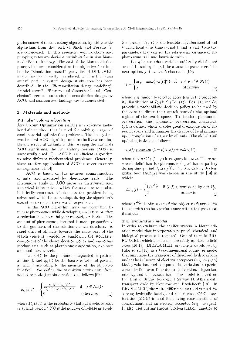
Figure 1. Initial contaminant plume location andunmanaged condition after 5 years.

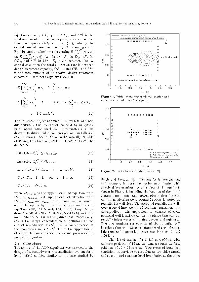
Figure 2. Insitu bioremediation system [9].

Shieh and Peralta [9]. The aquifer is homogenousand isotropic. It is assumed to be contaminated withdissolved hydrocarbon. A plan view of the aquifer isshown in Figure 1, including the location of the initialcontaminant plume, unmanaged plume after 5 years,and the monitoring wells. Figure 2 shows the potentialremediation well sites. The potential remediation wellswere grouped into two sets of locations; upgradient anddowngradient. The upgradient set consists of sevenpotential well locations within the plume that can po-tentially inject water containing oxygen and nutrients.The downgradient set consists of six potential welllocations that can extract contaminated groundwater.Injection and extraction rates are between 0 and1:26 L/s.

The size of this aquifer is 510 m � 690 m, withan average depth of 15 m. In plan, a square uniformgrid size of 19 � 25 is used. Two types of boundarycondition, impervious or zero ux at two sides (northand south), and constant head boundaries at the other


Table 1. Input parameters of simulation model [9].

Input parameters Value

Grid size 19� 25

Cell size 30 m�30 m

Hydraulic conductivity 6� 10�5

Longitudinal dispersivity 10 m

Transverse dispersivity 2 m

E�ective porosity 0:3

Retardation factor 1

Anisotropy factor 1

Injected oxygen concentration 8 ppm

Background oxygen concentration 8 ppm

Remedial time 3 years

two sides (west and east), are speci�ed. The e�ectiveporosity of the soil is taken as 0:3. It is assumedthat there is no recharge throughout the area of theaquifer. Groundwater ow simulation is steady stateand the general direction of ow is from the west tothe east boundary. The values of �xed head boundariesat west and east are, 30:5 and 27:7 m, respectively.Along the left and right boundaries, the contaminantconcentration was set to 0 mg/L. The details of thehydraulic conductivity and initial plume are describedin Table 1.

Preliminary analysis shows that the plume willreach downgradient monitoring wells after 5 years, andnatural aerobic decay reduces the total contaminantmass by only 16%. In the contaminant plume area,initial oxygen concentration is zero because of aerobicbiodegradation. The remainder of the aquifer areahas 5 ppm oxygen concentration. The injected oxygenthrough the well is 8 ppm. Upper and lower boundson the hydraulic head for the injection wells are 33:5and 27:7 m, respectively, and the upper and lowerbounds on the hydraulic head for the extraction wellsare 30:5 and 24:4 m, respectively. The remediationperiod is 3 years and the cleanup target concentrationfor contaminant, Ctr, is 3 ppm for the entire study area.To avoid unacceptable plume spreading because of toomuch water injection, additional monitoring wells areinstalled at the other sides of the aquifer accordingto Figure 2. The maximum allowable contaminantconcentration in monitoring wells, Cal, is 1 ppm. Ta-ble 2 lists the cost coe�cients related to bioremediationsystem costs.

2.5. Model setupThe proposed modeling structure has been setup fortwo di�erent schemes; namely, schemes A and B.Scheme A assumes a uniform pumping rate fromeach well for the entire remediation horizon, whereas,in scheme B, pumping rates are permitted to vary

Table 2. Cost function coe�cient [9].

Coe�cient Value

ir 0:05Cp for injection cost 4; 755 ($ per L/s-year)Cp for extraction cost 15; 850 ($ per L/s-year)CIP 12; 000

D

D1.26 L/s=$ 20,000D2.52 L/s=$ 24,000D3.79 L/s=$ 28,000D5.05 L/s=$ 32,000D6.31 L/s=$ 36,000D7.53 L/s=$ 40,000D8.83 L/s=$ 44,000

E

E1.26 L/s=$ 30,000E2.52 L/s=$ 38,000E3.79 L/s=$ 46,000E5.05 L/s=$ 54,000E6.31 L/s=$ 62,000E7.57 L/s=$ 70,000

dynamically during the remediation horizon. SchemeA has 13 di�erent decision variables, of which 7 wellsare injection and the remaining 6 are discharge wells.Due to the discrete nature of the proposed ant colonyoptimization algorithm, the decision space for injectionand extraction wells has been discreted with uniformincrements ranging from zero to 1:26 L/s. Realizingthe number of decision variables of the discretizationscheme, the search space will contain 713 options, whichmay be classi�ed as a medium size problem.

Scheme B assumes di�erent injection and/or ex-traction rates in each period for each well. Therefore,for scheme B, there are 78 decision variables. In thiscase, the search space will contain 778 di�erent options.

In scheme A, values of 1, 0, 0.1, 1, 0.9 for thebasic tunable parameters, namely, �, �, �, �0 andq0, were set to the best values of previously reportedones [14,15,21]. Mentioned parameters for schemeB are presented in Table 3. A total number of110 and 350 ants were used, with 60, 300 iterationsfor schemes A and B, respectively. To improve thequality of the solutions and reduce the chance of beingtrapped in local optimums, pheromone re-initiation(PRI) and Partial Path Replacement (PPR) strategies,as recommended by Hon et al. [20], and PheromonePromotion (PP) strategies, as recommended by Jalaliet al. [21], were employed.

PRI is used when the possibility of stagnation isincreased (i.e., for a pre-de�ned number of iterations,no improvement is achieved). Pheromone concentra-tions in all paths are reinitialized by setting themequal to the initial value, �0. After pheromone re-


Table 3. Input parameters of ant colony algorithm.

Description Scheme A Scheme B

Number of ants (ant) 110 350

Internal iteration (itr) 60 300

Initial pheromone (�0) 1 1

Pheromone evaporation (�) 0.1 0.1

Control parameter (�) 1 1

Control parameter (�) 0 0

Tunable parameter (q0) 0.8 0.9

initiation, the search continues as normal. The PPRemployed in the present algorithm is based on randomdisplacement of some components of pairs of solutionsin each iteration. To reduce computational time, ineach iteration, a number of ants are chosen and partsof their solutions are randomly displaced with thoseof the global best from the beginning of the trail. APheromone Promotion (PP) mechanism is used to pre-vent falling in local optima. Due to pheromone deposi-tion and evaporation, a rapid convergence syndrome orstagnation problem may prevail, if no improvement isgained after a few iterations. So, if a new solution withan improved objective value is identi�ed, its pheromonemust be promoted to the maximum existing pheromoneconcentration (i.e., available global best solution). Ifthe existing pheromone concentration is very low, suchan improved solution may not be desirable for theagents to follow.

3-opt is a local search procedure that is usedto generate new solutions with mutations of the bestever solution produced at three decision points. Inthis research, the three optimization approach (3-opt),recommended by Dorigo and Gambaldella [15], is usedas another strategy to improve local search.

A simple ow diagram of the proposed simulation-optimization approach for the optimal design of agroundwater remediation system is depicted in Fig-ure 3.

3. Results and discussion

3.1. Static pumping strategy (scheme A)In all cases, the results represent the best policy foundfrom each set of replicates. All the designs discussedmeet all constraints, including the water quality con-

Figure 3. ACS algorithm for groundwater bioremediationsystem.

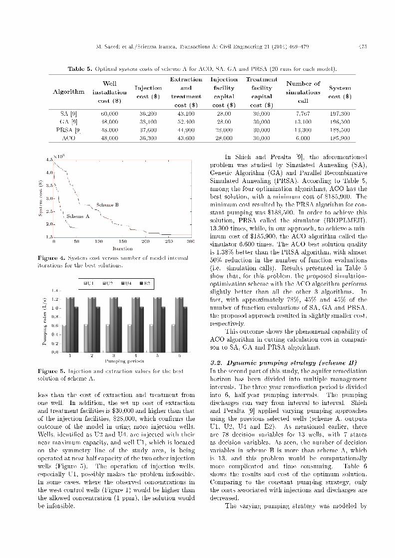
straint. Because of the stochastic nature of ACO, 20di�erent runs are performed for each setting. The best,worst, and average values of the objective function for20 runs, as well as standard deviation for the solutions,are presented in Table 4. Figure 4 illustrates theconvergence behavior of the proposed ACO algorithmfor the best solution. It shows the change of systemcost versus number of ACO internal iterations. Resultsfrom Table 5 show that the minimum cost in theconstant pumping strategy, for scheme A, would be$185, 900, resulted by selecting 4 wells (U1, U2, U4 andE2). According to Table 5, in scheme A, extractionand treatment operations through well E2 have thelargest portion of cost, by $43,600, and the cost ofthe other 3 injection wells is $36,300. The cost ofoxygen and nutrient injections in the three wells is

Table 4. Optimal system costs for Scheme A and B.

Formulation Mean Thebest

Theworst

S.D. C. V. Number of modelruns

Scheme A 191.4 185.9 200.2 4.8 0.02 20Scheme B 164.8 161.2 170.1 2.5 0.02 10


Table 5. Optimal system costs of scheme A for ACO, SA, GA and PRSA (20 runs for each model).

AlgorithmWell

installationcost ($)

Injectioncost ($)

Extractionand

treatmentcost ($)

Injectionfacilitycapitalcost ($)

Treatmentfacilitycapitalcost ($)

Number ofsimulations

call

Systemcost ($)

SA [9] 60,000 36,200 43,100 28,00 30,000 7,767 197,300GA [9] 48,000 38,100 52,400 28,00 30,000 13,100 196,500

PRSA [9] 48,000 37,600 44,900 28,000 30,000 13,300 188,500ACO 48,000 36,300 43,600 28,000 30,000 6,000 185,900

Figure 4. System cost versus number of model internaliterations for the best solutions.

Figure 5. Injection and extraction values for the bestsolution of scheme A.

less than the cost of extraction and treatment fromone well. In addition, the set up cost of extractionand treatment facilities is $30,000 and higher than thatof the injection facilities, $28,000, which con�rms theoutcome of the model in using more injection wells.Wells, identi�ed as U2 and U4, are injected with theirnear maximum capacity, and well U1, which is locatedon the symmetry line of the study area, is beingoperated at near half capacity of the two other injectionwells (Figure 5). The operation of injection wells,especially U1, possibly makes the problem infeasible.In some cases, where the observed concentrations inthe west control wells (Figure 1) would be higher thanthe allowed concentration (1 ppm), the solution wouldbe infeasible.

In Shieh and Peralta [9], the aforementionedproblem was studied by Simulated Annealing (SA),Genetic Algorithm (GA) and Parallel RecombinativeSimulated Annealing (PRSA). According to Table 5,among the four optimization algorithms, ACO has thebest solution, with a minimum cost of $185,900. Theminimum cost resulted by the PRSA algorithm for con-stant pumping was $188,500. In order to achieve thissolution, PRSA called the simulator (BIOPLMEII),13,300 times, while, in our approach, to achieve a min-imum cost of $185,900, the ACO algorithm called thesimulator 6,600 times. The ACO best solution qualityis 1:38% better than the PRSA algorithm, with almost50% reduction in the number of function evaluations(i.e. simulation calls). Results presented in Table 5show that, for this problem, the proposed simulation-optimization scheme with the ACO algorithm performsslightly better than all the other 3 algorithms. Infact, with approximately 78%, 45% and 45% of thenumber of function evaluations of SA, GA and PRSA,the proposed approach resulted in slightly smaller cost,respectively.

This outcome shows the phenomenal capability ofACO algorithm in cutting calculation cost in compari-son to SA, GA and PRSA algorithms.

3.2. Dynamic pumping strategy (scheme B)In the second part of this study, the aquifer remediationhorizon has been divided into multiple managementintervals. The three-year remediation period is dividedinto 6, half-year pumping intervals. The pumpingdischarges can vary from interval to interval. Shiehand Peralta [9] applied varying pumping approachesusing the previous selected wells (scheme A, outputsU1, U2, U4 and E2). As mentioned earlier, thereare 78 decision variables for 13 wells, with 7 statesas decision variables. As seen, the number of decisionvariables in scheme B is more than scheme A, whichis 13, and this problem would be computationallymore complicated and time consuming. Table 6shows the results and cost of the optimum solution.Comparing to the constant pumping strategy, onlythe costs associated with injections and discharges aredecreased.

The varying pumping strategy was modeled by


Table 6. Optimal system costs of scheme B for ACO and PRSA (10 runs for each formulation).

AlgorithmWell

installationcost ($)

Injectioncost ($)

Extractionand

treatmentcost ($)

Injectionfacilitycapitalcost ($)

Treatmentfacilitycapitalcost ($)

Number ofsimulations

call

Systemcost ($)

ACO 48,000 24,400 30,800 28,000 30,000 105,000 161,200PRSA [9] 48,000 25,800 31,500 28,000 30,000 NA� 163,300

* Not assigned.

Table 7. Injection and extraction rates of the best solutions of schemes A and B.

Wells Injection rates (lit/sec) Extraction rates (lit/sec)

U1 U2 U3 U4 U5 U6 U7 E1 E2 E3 E4 E5 E6Scheme A One period 0.63 1.26 0 1.25 0 0 0 0 1.05 0 0 0 0

Scheme B

Period 1 0.42 1.26 0 1.26 0 0 0 0 0 0 0 0 0

Period 2 0.42 1.26 0 1.26 0 0 0 0 0 0 0 0 0

Period 3 0 1.26 0 1.26 0 0 0 0 0.84 0 0 0 0

Period 4 0 0.84 0 0.84 0 0 0 0 1.05 0 0 0 0

Period 5 0 0 0 0 0 0 0 0 1.26 0 0 0 0

Period 6 0 0 0 0 0 0 0 0 1.26 0 0 0 0

Shieh and Peralta [9] using the PRSA optimizationalgorithm, resulting in a minimum cost of $163,300.The authors indicate they have used a populationsize of 200, instead of 100, in the constant pumpingproblem. However, they did not mention the numberof function evaluations or BIOPLUMEII calls. Sincethe problem is more complicated than the previousone, for PRSA formulation, the number of simulationcalls greatly exceeds that of the static case (i.e.,13,300).

Results of the proposed scheme selects threeinjection wells, U1, U2, U4, and one extraction well,E2, as the optimum decision. According to Table 6,the minimum cost for the selected solution is $161,200,which is slightly (1:3%) better than the PRSA outcome.The reported near optimum solution was achieved with105,000 function evaluations (i.e., simulation calls).The convergence behavior of the proposed ACO algo-rithm for the best solution of scheme B is illustrated inFigure 4.

The minimum cost obtained in the dynamicpumping strategy (scheme B) is 13:3% better thanthe static pumping (scheme A). In various stages ofthe remediation process, operation discharges varyby contamination concentration changes (Figure 6).According to Table 7, injection wells are super activeduring the �rst 4 operational intervals (�rst two years),in which wells U2 and U4 should be used with almostfull capacity. In addition, during the last year ofoperation, the discharge rate of injection wells is zero.It shows that during the last two periods, contamina-tion has moved downstream, and the injection process

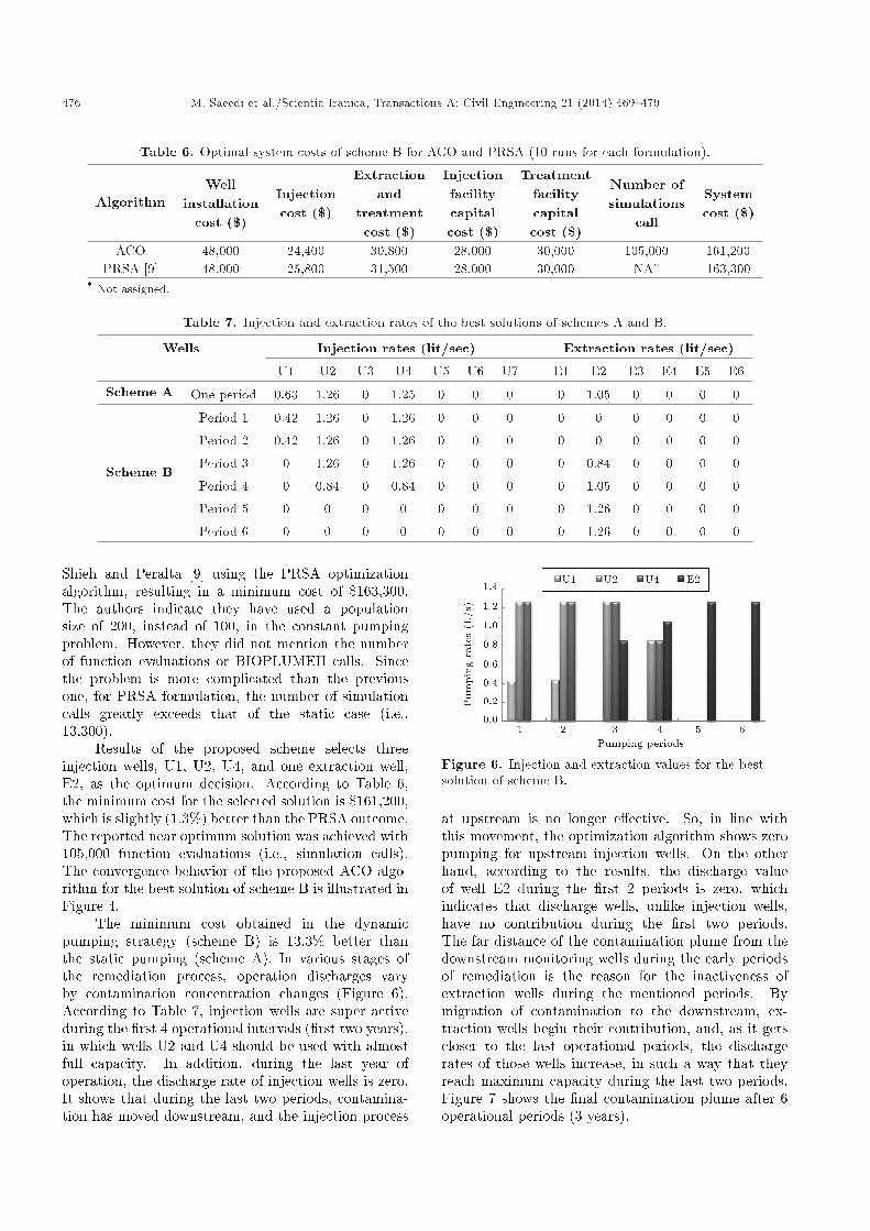
Figure 6. Injection and extraction values for the bestsolution of scheme B.

at upstream is no longer e�ective. So, in line withthis movement, the optimization algorithm shows zeropumping for upstream injection wells. On the otherhand, according to the results, the discharge valueof well E2 during the �rst 2 periods is zero, whichindicates that discharge wells, unlike injection wells,have no contribution during the �rst two periods.The far distance of the contamination plume from thedownstream monitoring wells during the early periodsof remediation is the reason for the inactiveness ofextraction wells during the mentioned periods. Bymigration of contamination to the downstream, ex-traction wells begin their contribution, and, as it getscloser to the last operational periods, the dischargerates of those wells increase, in such a way that theyreach maximum capacity during the last two periods.Figure 7 shows the �nal contamination plume after 6operational periods (3 years).


Figure 7. Change of contaminant plume (ppm) after 3years bioremediation in scheme B.

4. Conclusion

In this research, an improved ant colony optimizationmodel has been employed to optimize the in situ biore-mediation design system. The model is coupled with asimulator called BIOPLUMEII. Decision variables inthe simulation/optimization model are the pumpingvalues of injection and extraction wells, and the loca-tion of wells. The objective function is minimizationof total system cost. Reduction of contaminant tothe cleanup standard is a target in this problem. PP,PRI, PPR and 3-opt mechanisms have been employedto improve the convergence and performance of ACOalgorithm, so called ACSgb-PP-PRI-PPR-3opt.

ACSgb-PP-PRI-PPR-3opt was compared withGA, SA and PRSA in scheme A and with PRSA inscheme B. The scheme A problem has been solvedwith steady, and scheme B with time varying, pumpingstrategies. The number of simulations in the ACOis less than the other mentioned algorithms in bothschemes. Also, the quality of solutions in ACO is bettertoo.

Results of this research show the ability of the pro-posed ACO algorithm in the computationally expensiveproblem of groundwater bioremediation system design,and show that it can be used as a method for enablingthe solution of larger-scale groundwater remediationdesign problems.

Nomenclature

�ij(t) Total pheromone deposited on path ijat time t

�ij(t) Heuristic value of path ij at time tNk(t) Feasible neighborhood of ant k when

located at time period tNC Number release intervals (or classes)

� Control parameter of pheromone trail� Control parameter of heuristic valueq Random variable uniformly distributed

over [0,1]q0 Tunable parameter 2 [0,1]� Pheromone evaporation coe�cient�0 Initial pheromone value

Gk�gb Value of the objective function for the

ant with the best performance withinthe past total iterations

C and O2 Contaminant and oxygen concentrationin aquifer

C 0 and O02; Contaminant and oxygen concentrationin a source or sink uid

ne E�ective porosityb Aquifer saturated thicknesst Timexi and xj Cartesian coordinatesW Volume ux per unit areaVi Seepage velocity in the direction of xiRc Retardation factorDij Hydrodynamic dispersion coe�cient�CRC ;�CRO2 Change in contaminant and oxygen

concentrationsF Ratio of consumed oxygen to consumed

contaminantir Discount rateyP Stress period duratione Index of potential injection or

extraction locationp(e; t) Injection or extraction rate at location

e for stress period tCp(e) Cost coe�cient for injection or

extractionMn Total number of stress periodsMp Total number of wellsCIP Well installation cost at location eIP (e) Zero-one integer variable for well

existence at location eM i Total number of injection wellsMe Total number of extraction wellsDq; Eq Capital cost of injection and extraction

facilities at di�erent levelCDq; CEq Design injection and extraction

capacity at level q

MQ Total number of alternative designinjection capacities

Qmax inj Upper bound of injection ratesQmax ext Upper bound of extraction rates


hmin; hmax Minimum and maximum allowableaquifer hydraulic heads at wells

m;n Number of cells in x and y directionsCtr Target concentration of pollutant at

the end of remediationCm Concentration at the monitoring wellsCal Upper bound of allowable

concentration Set of monitoring wells

References

1. Zou, Y., Huang, G.H., He, L. and Li, H. \Multi-stageoptimal design for groundwater remediation: A hybridbi-level programming approach", J. Contam. Hydrol.,108(1-2), pp. 64-76 (2009).

2. Atwood, D.F. and Gorelick, S.M. \Hydraulic gradientcontrol for groundwater contaminant removal", J.Hydrol., 76, pp. 85-106 (1985).

3. McKinney, D.C. and Lin, M.D. \Pump-and-treatground-water remediation system optimization", J.Water Res. Pl. and Mg., 122(2), pp. 128-136 (1996).

4. Culver, T.B. and Shoemaker, C.A. \Dynamic optimalcontrol for groundwater remediation with exible man-agement periods", Water Resour. Res., 28(3), pp. 629-641 (1992).

5. Rizzo, D.M. and Dougherty, D.E. \Design optimiza-tion for multiple management period groundwaterremediation", Water Resour. Res., 32(8), pp. 2549-2561 (1996).

6. Chan Hilton, A.B. and Culver, T.B. \Constrainthandling for genetic algorithms in optimal remediationdesign", J. Water Res. Pl. and Mg., 126(3), pp. 128-137 (2000).

7. Minsker, B.S. and Shoemaker, C.A. \Dynamic optimalcontrol of in situ bioremediation of ground water", J.Water Res. Pl. and Mg., 124(3), pp. 149-161 (1998).

8. Dorigo, M. \Optimization, learning and natural algo-rithms", Ph.D. Thesis, Politecnico di Milano, Milan,Italy (1992).

9. Shieh, H.J. and Peralta, R.C. \Optimal in situbioremediation design by hybrid genetic algorithm-simulated annealing ", J. Water Res. Pl. and Mg.,131(1), pp. 67-78 (2005).

10. Dorigo, M. and Gambardella, L.M. \Ant colonies forthe traveling salesman problem", BioSystems, 43, pp.73-81 (1997a).

11. Li, Y. and Chan Hilton, A.B. \Optimal groundwatermonitoring designs using an ant colony optimizationparadigm", Environ. Modell. Softw., 22(1), pp. 110-116 (2007).

12. Maier, H.R., Simpson, A.R., Zecchin, A.C., Foong,W.K., Phang, K.Y., Seah, H.Y. and Tan, C.L. \Antcolony optimization for design of water distribution

systems", J. Water Res. Pl. and Mg, 129(3), pp. 200-209 (2003).

13. Zecchin, A.C., Simpson, A.R. and Maier, H.R. \Para-metric study for ant algorithms applied to waterdistribution system optimization", IEEE T Evolut.Comput., 9(2), pp. 175-191 (2005).

14. Jalali, M.R., Afshar, A. and Marino, M.A. \Optimumreservoir operation by ant colony optimization algo-rithms", Iran J. Sci. and Technol., 30(B1), pp. 107-117(2006).

15. Dorigo, M., Gambardella, L.M. \Ant colony system: Acooperative learning approach to the traveling sales-man problem", IEEE T. Evolut. Comput., 1(1), pp.53-66 (1997b).

16. Burges, K.S., Rifai, H.S. and Bedient, P.B. \Flowand transport modeling of a heterogeneous �eld sitecontaminated with dense chlorinated solvent waste",Proceedings of the Petroleum Hydrocarbons and Or-ganic Chemicals in Groundwater: Prevention, Detec-tion, and Restoration, American Petroleum Instituteand NGWA, Houston, Texas, pp. 693-707 (1993).

17. Wiedemeier, T.H., Wilson, J.T., Miller, R.N. andCampbell, D.H. \United air force guidelines for suc-cessfully supporting intrinsic remediation with an ex-ample from hill air force base", Proceeding of thePetroleum Hydrocarbons and Organic Chemicals inGroundwater: Prevention, Detection, and Restoration:NGWA and American Petroleum Institute, Houston,Texas, pp. 317-334 (1994).

18. Rifai, H.S., Bedient, P.B., Wilson, J.T., Miller, K.M.and Armstrong, J.M. \Biodegradation modeling at avi-ation fuel spill site", J. Environ. Eng. ASCE, 114(5),pp. 1007-1029 (1988).

19. Konikow, L.F. and Bredehoeft, J.D. \Computer modelof two dimensional solute transport and dispersionin ground water", Techniques of Water ResourcesInvestigation of the USGS, Washington, D.C. (1978).

20. Hon, M., Jalali, M.R., Afshar, A. and Marino, M.A.\Multi-reservoir operation by adaptive pheromone re-initiated ant colony optimization algorithm", Intern.J. Civil Eng., 5(4), pp. 284-301 (2007).

21. Jalali, M.R., Afshar, A. and Marino, M.A. \Improvedant colony optimization algorithm for reservoir opera-tion", Sci. Iran, Vol., 13(3), pp. 295-302 (2006).

Biographies

Mohsen Saeedi obtained his BS degree in ChemicalEngineering and MS degree in Civil and Environ-mental Engineering from Iran University of Scienceand Technology (IUST), Tehran, Iran. He receivedhis PhD degree in Environmental Engineering fromthe University of Tehran, Iran. He is currentlyAssociate Professor of Environmental Engineering atthe School of Civil Engineering, IUST. His research


interests include geo-environmental engineering andscience, physical-chemical treatment processes, wastemanagement, soil and sediment pollution and remedi-ation.

Abbas Afshar obtained his BS degree in Irrigationand Drainage from Tehran University, Iran, and MSand PhD degrees in Civil Engineering from the Univer-sity of California, Davis, USA. He is currently Professorof Civil Engineering at the School of Civil Engineeringat Iran University of Science and Technology (IUST),Tehran, Iran. His research interests include hydro-system engineering and management, risk and uncer-tainty analysis, reliability based optimum design and

operation, environmental impact assessment and waterquality modeling and management.

Hojjat Hosseinzadeh obtained his BS degree inCivil Engineering from Iran University of Scienceand Technology (IUST), Tehran, Iran, and his MSdegree in Civil Engineering from Tabriz University,Iran. He is currently a PhD degree student in CivilEngineering at IUST, and a civil supervisor at MahabGhods Consulting Engineering Company, Tehran, Iran.His research interests include geo-environmental engi-neering, physical-chemical treatment modeling, waterresource management, water quality modeling andmanagement.

Date post:	14-May-2018
Category:	Documents
Upload:	duongkien
View:	219 times
Download:	1 times

Multi-period aerobic groundwater bioremediation system design; ACO...

Documents