HAL Id: hal-00796581https://hal.archives-ouvertes.fr/hal-00796581v2

Submitted on 8 Nov 2013

HAL is a multi-disciplinary open accessarchive for the deposit and dissemination of sci-entific research documents, whether they are pub-lished or not. The documents may come fromteaching and research institutions in France orabroad, or from public or private research centers.

L’archive ouverte pluridisciplinaire HAL, estdestinée au dépôt et à la diffusion de documentsscientifiques de niveau recherche, publiés ou non,émanant des établissements d’enseignement et derecherche français ou étrangers, des laboratoirespublics ou privés.

Multi-revolution composition methods for highlyoscillatory differential equations

Philippe Chartier, Joseba Makazaga, Ander Murua, Gilles Vilmart

To cite this version:Philippe Chartier, Joseba Makazaga, Ander Murua, Gilles Vilmart. Multi-revolution compositionmethods for highly oscillatory differential equations. Numerische Mathematik, Springer Verlag, 2014,128 (1), pp.167-192. 10.1007/s00211-013-0602-0. hal-00796581v2

Multi-revolution composition methods for highly oscillatory

differential equations

Philippe Chartier1, Joseba Makazaga2, Ander Murua2, and Gilles Vilmart3,4

November 4, 2013

Abstract

We introduce a new class of multi-revolution composition methods (MRCM) for the

approximation of the Nth-iterate of a given near-identity map. When applied to thenumerical integration of highly oscillatory systems of differential equations, the techniquebenefits from the properties of standard composition methods: it is intrinsically geomet-ric and well-suited for Hamiltonian or divergence-free equations for instance. We proveerror estimates with error constants that are independent of the oscillatory frequency.Numerical experiments, in particular for the nonlinear Schrodinger equation, illustratethe theoretical results, as well as the efficiency and versatility of the methods.

Keywords: near-identity map, highly-oscillatory, averaging, differential equation, com-position method, geometric integration, asymptotic preserving.

MSC numbers: 34K33, 37L05, 35Q55.

1 Introduction

In this paper, we are concerned with the approximation of the N -th iterates of a near-identity smooth map by composition methods. More precisely, considering a smooth map(ε, y) 7→ ϕε(y) of the form

ϕε(y) = y + εΘε(y), (1)

we wish to approximate the result of N = O(1/ε) compositions of ϕε with itself

ϕNε = ϕε · · · ϕε

︸ ︷︷ ︸

N times

(2)

with the aid of a method whose efficiency remains essentially independent of ε.In order to motivate our composition methods, it will be useful to observe that ϕε can be

seen as one step with step-size ε of a first order integrator for the differential equation

dz(t)

dt= Θ0(z(t)), (3)

1INRIA Rennes, IRMAR and ENS Cachan Bretagne, Campus de Beaulieu, F-35170 Bruz, France.Philippe.Chartier@inria.fr

2Konputazio Zientziak eta A. A. Saila, Informatika Fakultatea, UPV/EHU, E-20018 Donostia – San Se-bastian, Spain. Ander.Murua@ehu.es, Joseba.Makazaga@ehu.es

3Ecole Normale Superieure de Cachan, Antenne de Bretagne, INRIA Rennes, IRMAR, CNRS, UEB, av.Robert Schuman, F-35170 Bruz, France. Gilles.Vilmart@bretagne.ens-cachan.fr

4Present address: Universite de Geneve, Section de mathematiques, 2-4 rue du Lievre, CP 64, 1211 Geneve4, Switzerland

1

where Θ0(z) = ddεϕε(z)

∣∣ε=0

, and thus, ϕNε (y) may be interpreted as an approximation at

t = Nε of the solution z(t) of (3) with initial condition

z(0) = y. (4)

A standard error analysis shows that ϕNε (y) − z(Nε) = O(εH) as H = Nε → 0, which

makes clear that, for sufficiently small H = εN , ϕNε (y) could be approximated by one step

ΨH(y) ≈ z(H) of any pth order integrator applied to the initial value problem (3)–(4) withinan error of size O(Hp+1 + εH). In particular, ϕH can be seen as a first order integrator forthe ODE (3), and a second order integrator can be obtained as

ΨH(y) = ϕH/2 ϕ∗H/2(y), (5)

where ϕ∗ε := ϕ−1

−ε is the adjoint map of ϕε. More generally, one could consider pth ordercomposition integrators of the form [21]

ΨH(y) := ϕa1H ϕ∗b1H · · · ϕasH ϕ∗

bsH(y) ≈ z(H) (6)

with suitable coefficients ai, bi (see for instance [16, 22] for particular sets of coefficientschoosen for different s and p), that would provide an approximation

ΨH(y) = z(H) +O(Hp+1) = ϕNε (y) +O(Hp+1 + εH)

for H = Nε → 0. However, the accuracy of the approximation is limited by the givenvalue of the problem parameter ε being sufficiently small. Motivated by that, we generalizethe approximation (6) by replacing the real numbers ai, bi (j = 1, . . . , s) by appropriatecoefficients αj(N), βj(N) depending on N , chosen in such a way that ϕN

ε is approximatedfor sufficiently small H = Nε within an error of size O(Hp+1), where the error constant isindependent of N,H, ε. We will say that such a method

ΨN,H(y) := ϕα1(N)H ϕ∗β1(N)H · · · ϕαs(N)H ϕ∗

βs(N)H(y) (7)

is an s-stage pth order multi-revolution composition method (MRCM) if

ΨN,H(y) = ϕNε (y) +O(Hp+1), for H = Nε→ 0. (8)

For instance, we will see that the second order standard composition method (5) can bemodified to give a second order MRCM (7) with s = 1, α1(N) = (1 +N−1)/2, and β1(N) =(1−N−1)/2,

ΨN,H(y) = ϕα1(N)H ϕ∗β1(N)H(y) = ϕN

ε (y) +O(H3), for H = Nε→ 0,

where the constant in O is independent of N and ε. It is interesting to observe that thissecond order MRCM reduces in the limit case N → ∞ to the standard composition method(5) (a second order integrator for the ODE (3)), which is consistent with the fact that ϕN

H/N

converges to the H-flow of (3) as N → ∞. More generally, any pth order MRCM (7), givesrise to a pth order standard composition method (6) with

ai = limN→∞

αi(N), bi = limN→∞

βi(N).

2

In practice, if one wants to approximately compute the map ϕMε for a given small value of

ε and large positive integersM within a given error tolerance by means of a s-stage pth orderMRCM (7), then one should choose a sufficiently small step-size H to achieve the requiredaccuracy, and accordingly choose N as the integer part of H/ε, in order to approximateϕMε (y), for M = mN , m = 1, 2, 3 . . ., as

ϕmNε (y) ≈ ΨN,H(y)m.

These approximations will be computed more efficiently than actually evaluating ϕmNε (y) if

such a positive integer N is larger than 2s. The case where N is not larger than 2s is thustreated as follows: we define

ΨN,H(y) := ϕNε , for all 1 ≤ N < 2s. (9)

Since the error of multi-revolution methods essentially depends on H but not on ε, for aprescribed accuracy (which determines H), in the case N ≥ 2s, the computational cost maybe reduced by a factor of N/(2s) ≤ H/(2sε) which increases as ε decreases, while for N < 2sthe method is exact and corresponds to N standard compositions of the map ϕε. This lattercase means that the problem where ε > H/(2s) is not sufficiently highly oscillatory and thereis no need to resort to the multi-revolution approach.

We assume that the computational cost of computing ϕ∗ε = ϕ−1

−ε is similar to that ofcomputing ϕε. The main application we have in mind is the time integration of highly-oscillatory problems with a single harmonic frequency ω = 2π/ε. In the numerical examples,we consider in particular problems of the form

d

dty(t) =

1

εAy(t) + f(y(t)), 0 ≤ t ≤ T, y(0) = y0 ∈ R

d, (10)

where A is a d× d constant matrix with eA = I, so that etA is 1-periodic in time, and wheref : Rd → R

d is a given nonlinear smooth function. In this situation, we shall consider ϕε

as the flow with time ε (the period of the unperturbed equation corresponding to f(y) ≡ 0)of equation (10). In this case, observe that the adjoint ϕ∗

ε = ϕ−1−ε is the flow with time 1 of

the above system where A is replaced by −A (equivalently, the flow with time −ε of (10)with ε replaced by −ε). It is worth stressing that MRCMs can be applied to more generalhighly-oscillatory problems with a single harmonic frequency. This is the case of any problemthat, possibly after a change of variables, can be written into the form

d

dtz(t) = g(z(t), t/ε), 0 ≤ t ≤ T, z(0) = z0 ∈ R

d, (11)

where g(z, τ) is smooth in z and continuous and 1-periodic in τ . For instance, (10) can berecast into the format (11) with g(z, τ) = e−τ Af(eτ Az) by considering the change of variablesy = etA/εz. In this more general context, ϕε will be such that for arbitrary z0, the solutionz(t) of (11) satisfies that z(ε) = ϕε(z0).

It is well known [9, 10] that such a map ϕε is a smooth near-identity map, and furthermore,that (3) is in this case the first order averaged equation, more precisely,

Θ0(z) =d

dεϕε(z)

∣∣∣∣ε=0

=

∫ 1

0e−Atf(eAtz)dt.

3

The solution y(t) of the initial value problem (10) sampled at the times t = εM will then begiven by

y(εM) = ϕMε (y0),

and thus, for an appropriately chosen positive integer N (determined by accuracy require-ments and the actual value of ε), we may use a pth order MRCM (7) to compute the approx-imations

ym = ΨN,H(y)m ≈ ϕmNε (y0) = y(tm), where tm = mH, H = εN.

The local error estimate (8) then leads by standard arguments to a global error estimate ofthe form

ym − y(tm) = O(Hp), for tm = mH ≤ T,

where the constant in the O-term depends on T but is independent of ε and H.Typically, the maps ϕµ and ϕ∗

µ in (7) with µ = αj(N)H, µ = βj(N)H (j = 1, . . . , s) cannot be computed exactly. In the context of highly oscillatory systems, and in particular, forsystems of the form (10), the actual (approximate) computation of ϕµ can be carried outessentially as a black-box operation: In practice, one may use any available implementationof some numerical integrator to approximate the flow with time 1 of the ODE

d

dtu(t) = Au(t) + µf(u(t)). (12)

In particular, ϕµ may be approximated by applying n steps of step-size h = 1/n of anappropriate splitting method to (12), where n is chosen so as to resolve one oscillation. LetΦµ,h(y) denote the approximation of ϕµ obtained in this way with a qth order splittingmethod, then the following estimate

Φµ,h(y)− ϕµ(y) = O(µrhq) (13)

will be guaranteed to hold with r = 1.In the most general framework, we shall assume that, if ϕµ can not be computed exactly,

then it is approximated by some computable map Φµ,h (depending on a small parameter hthat controls the accuracy of the approximation) satisfying the error estimate (13) for somer ≥ 0 and q ≥ 1. Observe that one can expect r ≥ 1 in the right-hand side of (13) if (as inthe case of splitting methods for (12),) Φµ,h is constructed so that Φ0,h(y) = ϕ0(y) = y.

In what follows, the method (7) where the involved maps ϕµ and ϕ∗µ are assumed to be

computed exactly, will be referred to as semi-discrete multi-revolution composition methods.We next define the following fully-discrete version, in the spirit of Heterogenerous multiscalemethods (HMM) (see [1, 11, 12]) which combine the application of macro-steps of length H(to advance along the solution of (10)) with the application to (12) of some integrator withmicro-steps of size h = 1/n (where n is chosen large enough to resolve each oscillation).

Definition 1.1 (Fully-discrete multi-revolution composition methods). Let an integer s ≥ 1and a family of coefficients αj(N), βj(N) defined for j = 1, . . . , s and N ≥ 2s, and anapproximation Φε,h of ϕε. For the approximation of ϕN

ε , with ε > 0, N ≥ 1, we define ans-stage fully-discrete MRCM as the composition

ΨN,H,h(y) = Φα1(N)H,h Φ∗β1(N)H,h · · · Φαs(N)H,h Φ

∗βs(N)H,h(y) if N ≥ 2s,

ΨN,H,h(y) = ΦNε,h if N < 2s, (14)

where H = Nε and Φ∗ε,h := Φ−1

−ε,h is the adjoint map of Φε,h.

4

When solving a highly-oscillatory problem of the form (10) with standard numericalmethods, stability and accuracy requirements induce a step-size restriction of the form h ≤Cε which renders the computation of a reasonably accurate solution more and more costlyand sometimes even untractable for small values of ε. In contrast, we propose to use theapproximation Ψm

N,H(y) ≃ ϕMε (y) where εM ≤ T with T fixed, m,M,N ∈ N with Nε = H,

mN = M . Using for ΨN,H a MRCM (7) of order p, we prove that the error is ΨmN,H(y) −

ϕMε (y) = O(Hp) with a constant independent of m,N, ε. Given a prescribed accuracy Tol

which induces a stepsize H (H ≥ ε), setting N as the integer part of ε−1H, this permitsto approximate the solution with the accuracy Tol at a cost proportional to m = TH−1 ∼Tol−1/p which does not grow for small values of ε. Using the fully-discrete MRCM (14), thecost is scaled by the additional factor n = h−1, again independently of ε.

The general idea of multi-revolution methods has been first considered in astronomy,where ε-perturbation of periodic systems are recurrent, and named as such since these meth-ods approximate many revolutions (N periods of time) by only a few (in our approach, 2scompositions then accounts for 2s revolutions with different values of the perturbation pa-rameter ε). A class of multi-revolution Runge-Kutta type methods has then been studied inthe context of oscillatory problems of the form (10) in [3, 4, 23, 25] and [2] was the firstsystematic analysis of the order conditions of convergence. Closely related methods wereconsidered in [19] and also in [5].

Actually, MRCM are asymptotic preserving, a notion introduced in the context of kineticequations (see [18], and the recent works [20, 14]) and ensuring that a method is uniformlyaccurate for a large range of values of the parameter ε with a computational cost essentiallyindependent of ε. This is a feature shared by the proposed classes of multi-revolution methods.

The methods introduced in this paper differ from existing other multi-revolution methodsin that they are intrinsically geometric, since they solely use compositions of maps of the formϕµ and ϕ−1

µ , whose geometric properties are determined by equation (10). In particular, theyare symplectic if (10) is Hamiltonian, volume-preserving if (10) is divergence-free, and sharethe same invariants which are independent of ε as the flow of (10). This is also true in thefully-discrete version (14) provided that the micro-integrator Φµ,h used to approximate ϕµ

satisfy the required geometric properties.Deriving general order conditions for (7) requires to compare the Taylor expansions of

both sides of ΨN,H(y) ≃ ϕNε (y). Although conceptually easy, the task is rendered very

intricate by the enormous number of terms and redundant order conditions naturally arising.Explicit conditions for standard composition methods have been obtained in a systematic wayin [24] by using the formalism of B∞-series and trees. In the situation we consider here, themap ϕε is the flow with time ε of an ODE that depends on the parameter ε, and consequentlydoes not obey a group law. The question of approximating ϕN

ε/N by a composition of the

form (7) then makes perfect sense, and this article aims at analyzing the properties and orderconditions of such methods.

The paper is organized as follows. In Section 2, we derive the order conditions of the multi-revolution composition methods and perform a global error analysis of the methods. Section3 presents several methods of orders 2 and 4, and describes how they have been obtained.Section 4 is devoted to numerical experiments aimed at giving a numerical confirmation ofthe orders of convergence derived in Section 2 and to show the efficiency and versatility ofthe newly introduced methods.

5

2 Convergence analysis of MRCMs

In this section, we derive general order conditions for method (7) to approach ϕNε . There is a

complete analogy with order conditions of standard composition methods, with the exceptionthat the right-hand side of each condition is now depending on N . Prior to addressing thegeneral case, observe that the simplest method ϕH ≃ ϕN

ε with H = Nε, corresponds to s = 1,α1 = 1 and β1 = 0. As shown in the introduction, ϕH is the simplest approximation to ϕN

ε

in the following sense,

‖ϕH(y)− ϕNε (y)‖ ≤ CH2 for all 0 ≤ H = Nε ≤ H0.

Constructing high-order compositions soon becomes rather intricate, not to say undoable,unless one uses an appropriate methodology. This is precisely the object of the paper [24]which gives order conditions for standard composition methods explicitly. We will hereafterfollow the presentation of [16]. The starting point of this section is the Taylor series expansion1

ϕε(y) = y + εd1(y) + ε2d2(y) + ε3d3(y) + . . . (15)

of the smooth map (1).

2.1 Preliminaries: trees and B∞-series

In this subsection, we briefly recall the framework of B∞-series for the study of compositionmethods of the form

ϕαsε ϕ∗βsε · · · ϕα1ε ϕ

∗β1ε(y) (16)

originally developed for the numerical integration of equation (3) and yet completely relevantto the present situation. We thus define T∞ as the set of rooted trees where each vertex bears apositive integer and we denote 1 , 2 , 3 , . . . the trees with one vertex. Given τ1, . . . , τm ∈ T∞,we write as

τ = [τ1, . . . , τm]j (17)

the tree obtained by attaching the m roots of τ1, . . . , τm to a new root with label j. Inciden-tally, we define i(τ) = j the label beard by its root, |τ | = 1+ |τ1|+ . . .+ |τm| its number of ver-tices, ‖τ‖ = i(τ)+‖τ1‖+ . . .+‖τm‖ the sum of its labels2 and σ(τ) = µ1!µ2! · · ·σ(τ1) · · ·σ(τm)its symmetry coefficient, where µ1, µ2, . . . count equal trees among τ1, . . . , τm. Now, the B∞-series associated to a map a : T∞ ∪ ∅ → R is the formal series

B∞(a, ε, y) = a(∅)y +∑

τ∈T∞

ε‖τ‖

σ(τ)a(τ)F (τ)(y)

where the so-called “elementary differentials” are maps from U to Rd defined inductively by

the relations

F ( j )(y) = dj(y),

F ([τ1, . . . , τm]j)(y) = d(m)j (y)(F (τ1)(y), . . . , F (τm)(y)).

1Notice that d1(y) = Θ0(y).2By convention, |∅| = ‖∅‖ = 0.

6

We immediately see that the Taylor expansion (15) of ϕε can be considered as a B∞-series

ϕε(y) = y + εd1(y) + ε2d2(y) + ε3d3(y) + . . . = B∞(e1, ε, y)

with coefficients satisfying e1(τ) = 0 for all τ ∈ T∞ with |τ | > 1 and e1(∅) = 1, e1( j ) = 1for all j ∈ N

∗. As immediate is the obtention of the coefficients of the B-series expansion ofthe exact solution z(ε) of (3)

B∞(e∞, ε, y) = z(ε)

with coefficients e∞(τ) recursively defined3 by

e∞(∅) = 1, e∞(τ) =1

|τ |e′∞(τ) if i(τ) = 1, and e∞(τ) = 0 otherwise, (18)

where the prime stands for the following B-series operation: Given a : T∞ → R, the map a′

is defined recursively by

a′( j ) = 1 and for all τ = [τ1, . . . , τm]j ∈ T∞, a′(τ) = a(τ1) · · · a(τm).

We now quote the following fundamental result from [24]:

Lemma 2.1. The following compositions are B∞-series

ϕ∗βkε

· · · ϕα1ε ϕ∗β1ε(y) = B∞(bk, ε, y)

ϕαkε ϕ∗βkε

· · · ϕα1ε ϕ∗β1ε(y) = B∞(ak, ε, y)

with coefficients given recursively for all T ∈ T∞ by ak(∅) = bk(∅) = 1, a0(τ) = 0 and

bk(τ) = ak−1(τ)− (−βk)i(τ)b′k(τ) and ak(τ) = bk(τ) + α

i(τ)k b′k(τ).

In order to eliminate redundant order conditions, we finally fix as in [24] a total orderrelation < on T∞ compatible with | · |, i.e. such that u < v whenever |u| < |v|.

Definition 2.2. (Hall Set). The Hall set corresponding to the order relation < is the subsetH ⊂ T∞ defined by

(i) ∀j ∈ N, j ∈ H

(ii) τ ∈ H if and only if there exist u, v ∈ H,u > v, such that τ = u v.

Theorem 2.3. (Murua and Sanz-Serna [24]) Consider B(a, ε, y) and B(b, ε, y) two B∞-series obtained as compositions of the form (16) and let p ≥ 1. The following two statementsare equivalent:

(i) ∀τ ∈ T∞, ‖τ‖ ≤ p, a(τ) = b(τ),

(ii) ∀τ ∈ H, ‖τ‖ ≤ p, a(τ) = b(τ).

In the usual setting of composition methods, the previous theorem immediately givesthe reduced number of order conditions for order p by comparing the B∞-series B∞(a, ε, y)obtained from (16) and B∞(e∞, ε, y). In our context, we have to compare B∞(a, ε, y) withthe B∞-series of ϕN

ε . This is the purpose of the next section.

7

Order 1: 1

s∑

k=1

(αk + βk) = 1

Order 2: 2s∑

k=1

(α2k − β2k) = N−1

Order 3: 3s∑

k=1

(α3k + β3k) = N−2

2

1 s∑

k=1

(α2k − β2k)

k∑

ℓ=1

′(αℓ + βℓ) =N−1 −N−2

2

Order 4: 4

s∑

k=1

(α4k − β4k) = N−3

3

1 s∑

k=1

(α3k + β3k)

k∑

ℓ=1

′(αℓ + βℓ) =N−2 −N−3

2

2

1 1 s∑

k=1

(α2k − β2k)

( k∑

ℓ=1

′(αℓ + βℓ))2

=N−1(1−N−1)(2−N−1)

6

Order 5: 5

s∑

k=1

(α5k + β5k) = N−4

4

1 s∑

k=1

(α4k − β4k)

k∑

ℓ=1

′(αℓ + βℓ) =N−3 −N−4

2

3

2 s∑

k=1

(α3k + β3k)

k∑

ℓ=1

′(α2ℓ − β2ℓ ) =

N−3 −N−4

2

2

1 2 s∑

k=1

(α2k − β2k)

( k∑

ℓ=1

′(αℓ + βℓ))( k∑

ℓ=1

′(α2ℓ − β2ℓ )

)

=N−2(1−N−1)(2−N−1)

6

2

1 1 1 s∑

k=1

(α2k − β2k)

( k∑

ℓ=1

′(αℓ + βℓ))3

=N−1(1−N−1)2

4

3

1 1 s∑

k=1

(α3k + β3k)

( k∑

ℓ=1

′(αℓ + βℓ))2

=N−2(1−N−1)(2−N−1)

6

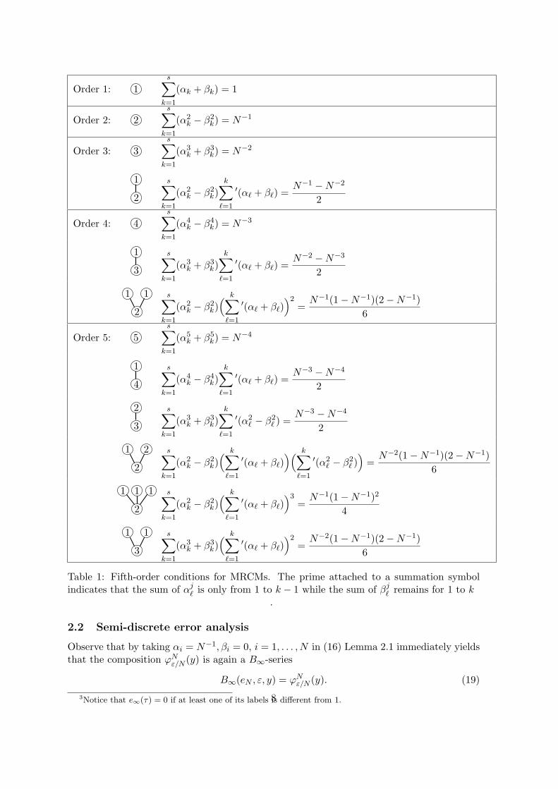
Table 1: Fifth-order conditions for MRCMs. The prime attached to a summation symbolindicates that the sum of αj

ℓ is only from 1 to k − 1 while the sum of βjℓ remains for 1 to k.

2.2 Semi-discrete error analysis

Observe that by taking αi = N−1, βi = 0, i = 1, . . . , N in (16) Lemma 2.1 immediately yieldsthat the composition ϕN

ε/N (y) is again a B∞-series

B∞(eN , ε, y) = ϕNε/N (y). (19)

3Notice that e∞(τ) = 0 if at least one of its labels is different from 1.8

Its coefficients eN (τ) can be computed by using the following lemma.

Lemma 2.4. For all N ∈ N∗, the coefficients eN (τ) of the B∞-series in (19) satisfy

∀j ∈ N∗, eN ( j ) = N1−j ,

∀τ = [τ1, . . . , τn]j ∈ T∞, N‖τ‖eN (τ) =N−1∑

k=1

k‖τ1‖+...+‖τn‖e′k(τ).

Proof. With αi = 1 and βi = 0, i = 1, . . . , N , Lemma 2.1 gives bk(τ) = ak−1(τ) and thus

aN (τ) =N∑

k=1

a′k−1(τ) =N−1∑

k=1

a′k(τ).

Using B∞(eN , ε, y) = B∞(aN , ε/N, y) yields aN (τ) = N‖τ‖eN (τ) and allows to conclude.

We obtain for instance eN ( 1 ) = 1, eN ( 2 ) = N−1 and

eN

(

1

1)=

1−N−1

2, eN

(

2

1)=N−1(1−N−1)

2, eN

(

2

1 1)=N−1(1−N−1)(2−N−1)

6.

Now, recalling that the map ϕε can be interpreted as a consistent integrator for equation (3),ϕNε/N (y0) converges to its solution z(ε) for N → ∞ and it is thus expected that the coefficients

eN (τ) converge to e∞(τ) as N → ∞. This is shown in next proposition.Consider now the B∞-series B∞(a, ε, y) associated to a semi-discrete MRCM of the form

(7) with H = ε. Writing the order conditions now boils down to comparing the coefficientsof B∞(a, ε, y) and B∞(eN , ε, y) and estimating the remainder term. Next lemma providesestimates of the derivatives of ϕN

ε w.r.t. ε. In order to alleviate the presentation, let usdenote for ρ > 0, Bρ(y0) = y ∈ R

d; ‖y− y0‖ ≤ ρ, and for a given function y 7→ k(y) definedon Bρ(y0),

‖k‖ρ := supy∈Bρ(y0)

‖k(y)‖ and ‖∂ny k‖ρ := supy ∈ Bρ(y0),

‖vi‖ = 1, i = 1, . . . , n

‖∂ny kε(y) (v1, . . . , vn) ‖.

Note that if (y, ε) 7→ Θε(y) in (1) is of class Cp+1 with respect to (y, ε) on the compact setBρ(y0)× [−ε0, ε0], then there exist positive constants K and L such that, for all |ε| ≤ ε0

‖∂yϕε‖ρ ≤ 1 + εL, ∀k = 2, . . . , p+ 1, ‖∂kyϕε‖ρ ≤ εL,

∀0 ≤ k + l ≤ p+ 1, ‖∂ky∂lεϕε‖ρ ≤ K.

Lemma 2.5. Assume that (y, ε) 7→ Θε(y) is defined and of class Cp+1 with respect to (y, ε)on B2R(y0) × [−ε0, ε0] for a given R > 0 and a given ε0 > 0. Then, there exists a constantH0 such that for all ε and N ≥ 1 with H = Nε ≤ H0,

∥∥∂p+1

ε ϕNε

∥∥R≤ CNp+1,

∥∥∥∂

p+1H ϕN

H/N

∥∥∥R≤ C, (20)

where C is independent of N and ε.

9

Proof. For y0 ∈ BR(y0) and denoting M := sup|ε|≤ε0 ‖Θε‖2R, we have

‖ϕNε (y0)− y0‖ ≤

N∑

k=1

‖ϕkε(y0)− ϕk−1

ε (y0)‖+ ‖y0 − y0‖ ≤ R+NεM

as long as the iterates ϕiε(y0) and ϕi

ε(y0) remain in B2R(y0) for 0 ≤ i ≤ N . Hence, ifNε ≤ H0 := min(R/M, ε0) then ‖ϕk

ε‖R ≤ 2R for all k = 0, . . . , N . Under this assumption,we now wish to prove by induction on n, that

∀n = 1, . . . , p+ 1,∥∥∂nε ϕ

Nε

∥∥R≤ CnN

n (21)

for some constants Cn independent of N, ε. Now, given a smooth function g : B2R(y0) → Rd

of class Cp+1, Faa di Bruno’s formula reads

∂kε (g ϕNε ) =

∑

m∈Nk, σ(m)=k

Bm g(|m|) ϕNε

(

(∂1εϕNε )m1 , . . . , (∂kεϕ

Nε )mk

)

where the sum is over all multi-indices m = (m1, . . . ,mk) of Nk such that k = σ(m) :=∑k

j=1 jmj and where |m| denotes m1 + . . .+mk and

Bm =k!

m1!1!m1 · · ·mk!k!mk.

We now use the differentiation formula

∂nε (ϕε ϕNε ) =

n∑

k=0

n!

k!(n− k)!∂kε (∂

(n−k)µ ϕµ ϕN

ε )∣∣∣µ=ε

and take g = ∂(n−k)µ ϕµ

∣∣∣µ=ε

in Faa di Bruno’s formula. This yields

∂nε (ϕN+1ε ) =

∑

0 ≤ k ≤ n,

m ∈ Nk, σ(m) = k

n!

k!(n− k)!Bm

(

∂|m|y ∂n−k

ε ϕε

)

ϕNε

(

(∂1εϕNε )m1 , . . . , (∂nε ϕ

Nε )mn

)

Hence, using the induction assumption, we get the estimates

∥∥∂nε ϕ

N+1ε

∥∥R

≤ ‖∂nε ϕε‖2R +∑

1 ≤ k ≤ n − 1,

m ∈ Nk, σ(m) = k

n!

k!(n− k)!Bm ‖∂|m|

y ∂n−kε ϕε‖2R

k∏

j=1

‖∂jεϕNε ‖

mj

R

+∑

m ∈ Nn, σ(m) = n,mn = 0

Bm ‖∂|m|y ϕε‖2R

n∏

j=1

‖∂jεϕNε ‖

mj

R + ‖∂yϕε‖2R‖∂nε ϕ

Nε ‖R

≤ K +KCn

n−1∑

k=1

Nk + εnCnLNn + (1 + εL)‖∂nε ϕ

Nε ‖R

≤ nKCn(N + 1)n−1 + nCnLH0Nn−1 + (1 + εL)‖∂nε ϕ

Nε ‖R

≤ Cn(N + 1)n−1 + (1 + εL)‖∂nε ϕNε ‖R

10

where the constants Cn and Cn are defined as

Cn = maxk=1,...,n−1

∑

m ∈ Nk

σ(m) = k

Bm

k∏

j=1

Cmj

j and Cn =∑

m ∈ Nn−1

σ(m) = n

Bm

n−1∏

j=1

Cmj

j

and Cn = nmax(K,KCn, CnLH0). Finally, using a standard discrete Gronwall lemma andH = Nε ≤ H0 yields

‖∂nε (ϕNε )‖R ≤ Cn

N∑

k=1

(1 + εL)N−kkn−1 ≤ CnNneLεN ≤ CnN

neLH0

which allows to conclude the proof of the first estimate in (20) by choosing Cn = CneLH0 in

(21). The second estimate is straightforwardly obtained through a change of variables.

We may now state the main result for the local error of the semi-discrete MRCM (7).

Theorem 2.6. Consider a semi-discrete MRCM (7)-(9) and assume further that its coeffi-cients αi(N), βi(N), i = 1, . . . , s are bounded with respect to N for all N ≥ 2s and satisfy

a(τ) = eN (τ), for all τ ∈ H with ‖τ‖ ≤ p, (22)

for a given order p ≥ 1. Then, there exist C,H0 > 0 such that for all H ≤ H0,

‖ΨN,H − ϕNε ‖R ≤ CHp+1

where H = Nε and the constants C,H0 are independent of N, ε.

Proof. Consider the two B∞-series B∞(a,H, y) and B∞(eN , H, y) associated respectively tothe semi-discrete MRCM (7) and to ϕN

H/N (y) in (19). It follows from Theorem 2.3 that these

B∞-series formally coincide up to order Hp. A Taylor expansion of ΨH(y) − ϕNH/N (y) with

integral remainder thus leads to

ΨN,H(y)− ϕNH/N (y) =

∫ H

0

1

p!(H − s)p

∂p+1Ψs

∂sp+1(y)ds−

∫ H

0

1

p!(H − s)p

∂p+1ϕNs/N

∂sp+1(y) ds.

The derivative∂p+1ϕN

s/N

∂sp+1 is bounded by Lemma 2.5. Given that coefficients αj , βj are uniformly

bounded with respect to N , ∂p+1Ψs∂sp+1 is bounded as well. We conclude using ϕN

H/N (y) = ϕNε (y).

We report in Table 1 order conditions up to order 5 as derived above. Note that Lemma2.4 implies (by induction) that the value of N‖τ‖eN (τ) is independent of the labels of thenodes of a given tree τ ∈ T∞. This explains why similar right-hand sides eN (τ) are obtainedfor trees where only labels differ.

Remark 2.7. For N → ∞, it can be shown that the coefficients of the B∞-series (19)satisfy eN (τ) → e∞(τ). This means that the order conditions (22) reduce for N → ∞ to theclassical order conditions of standard composition methods (16) for the approximation of theflow of (3), the averaged problem as ε→ 0.

11

Remark 2.8. It can be shown (see [26] and the recent work [9]) that the highly-oscillatorysolution of (10) is, at times which are integer multiples of the oscillatory period ε, asymptot-ically close to the solution of non-stiff averaged ODEs. Precisely, for all p ≥ 1, there exists asmooth ODE of the form

dz

dt= Θ0(z) + εG1(z) + · · ·+ εp−1Gp−1(z), z(0) = y0 (23)

whose solution z(t) satisfies z(Mε) − y(Mε) = O(εp) if Mε ≤ T, for all integer values ofM , where the constant in O is independent of ε. A similar statement can be made in thegeneral case of an arbitrary smooth near-identity map, where ϕε can be interpreted as aone-step integrator for the ODE (3), and (23) is the modified equation of (3) associated toϕε considered in backward error analysis of one step integrators [16, Chap. IX]. In addition,applying a pth order MRCM (7) to (10) (that is, (8) holds for integer values of N), it can beproved that for 0 < ε ≤ H with H → 0,

ΨH/ε,H(y0)− z(H) = O(Hp+1).

Note that in the above convergence estimate, H/ε in not necessarily an integer, which meansthat ΨN,H in (7) also makes sense for non-integer values of N .

2.3 Fully-discrete error analysis

In this subsection, we derive convergence estimates for fully-discrete MRCMs (14). We high-light once again that this is essential in view of applications because the exact computationof the map ϕε is not available in general and has to be approximated by a map Φh,ε.

Theorem 2.9. Assume that the hypotheses of Theorem 2.6 are fulfilled. Consider a fully-discrete MRCM (14) where the basic map Φh,ε is assumed to satisfy the accuracy estimate(13) for given q and r. Then there exist C,H0, h0 > 0 such that

‖ΨN,H,h − ϕNε ‖R ≤ C(Hp+1 +Hrhq)

for all H = Nε ≤ H0, h ≤ h0 and the constants C,H0, h0 re independent of N, ε, h.

As a consequence of Theorem 2.9, by standard arguments in the convergence analysisof one-step integrators, one gets a global error estimate for the numerical approximationsym = ΨN,H,h(ym−1) of problem (10) of the form

ym − y(mH) = O(Hp +Hr−1hq) for mH ≤ T.

For the proof of Theorem 2.9, we recall the following classical discrete Gronwall estimate.

Lemma 2.10. Let (φj , ψj), j = 1, . . . , k, be k couples of maps satisfying for ρ, ν > 0

‖φj(y)− ψj(y)‖ ≤ ρ, ‖φj(y1)− φj(y2)‖ ≤ (1 + ν)‖y1 − y2‖,

for all j = 1, . . . , k and all y, y1, y2. Then,

‖φk · · · φ1(y)− ψk · · · ψ1(y)‖ ≤ eνkkρ.

12

Proof. Let aj = φk · · · φk−j+1, bj = ψj · · · ψ1. We have

ak(y)− bk(y) =k−1∑

j=0

ak−j−1 φj+1 bj(y)− ak−j−1 ψj bj(y)

‖ak(y)− bk(y)‖ ≤k−1∑

j=0

(1 + ν)k−j−1‖φj+1 bj(y)− ψj+1 bj(y)‖ ≤ keνkρ

where we used the estimate∑k−1

j=0(1 + ν)k−j−1 ≤∑k−1

j=0 ejkνk ≤ k

∫ 10 e

νktdt ≤ keνk.

Proof of Theorem 2.9. We use the estimate

‖ΨN,H,h − ϕNε ‖R ≤ ‖ΨN,H,h −ΨN,H‖R + ‖ΨN,H − ϕN

ε ‖R

From Theorem 2.6, we have ‖ΨN,H − ϕNε ‖R ≤ CHp+1. The next estimate

‖ΨN,H,h −ΨN,H‖R ≤ CHrhq

is a consequence of Lemma 2.10 with k = 2s, ρ = CHrhq (using (13) with ε replaced byαj(N)H and βj(N)H), ν = O(ε) being a Lipsitz constant for the near-identity map ϕε, andφ2j−1 = ϕαj(N)H , φ2j = ϕ∗

βj(N)H , ψ2j−1 = Φh,αj(N)H , ψ2j = Φ∗h,βj(N)H .

2.4 Application to second order highly oscillatory systems

The multi-revolution approach can be applied to second order highly oscillatory systems ofthe form

q′′1(t) = g1(q1(t), q2(t), q′1(t)), q′′2(t) =

1

ε2Ω2q2(t) + g2(q1(t), q2(t), q

′1(t)), 0 ≤ t ≤ T, (24)

where we distinguish q1 and q2, respectively the smooth and highly oscillatory components.We denote y0 = (q1(0), q2(0), q

′1(0), q

′2(0)) the initial condition, Ω is a constant positive-

definite symmetric matrix with eigenvalues in 2πN∗ and g1, g2 are given smooth vector fieldswhich do not depend on the highly oscillatory velocity q′2(t). Such a form often appears forhighly oscillatory mechanical systems and an example is presented in Section 4.1. The mainobservation is that system (24) can be cast in the form (10) by setting y = (q1, q2, q

′1, q

′2)

T

and

A =

0 0 0 00 0 0 ηI0 0 0 00 −η−1Ω 0 0

, f(y) =

q′10

g1(q1, q2, q′1)

g2(q1, q2, q′1)

(25)

where η = ε is a fixed parameter. Then, the MRCM yields an uniformly accurate integratorfor (24) as stated in the following theorem for semi-discrete MRCMs. We highlight that aconvergence estimate for fully-discrete MRCMs could be derived analogously (see Theorem2.9).

13

Theorem 2.11. Consider y = (q1, q2, q′1, q

′2) the exact solution of (24) where we assume that

the vector fields g1, g2 have the regularity Cp+1. Consider ϕε the flow map with time ε of(10)-(25) where η = ε is fixed, and ΨN,H a MRCM (7) satisfying the hypotheses of Theorem2.6. Then, there exist C,H0 > 0 such that for all H ≤ H0, N ≥ 2s, and mH ≤ T ,

‖ΨmN,H(y0)− y(mH)‖ ≤ CHp,

where H = Nε and the constants C,H0 are independent of N, ε,m, η.

Proof. Using the variation of constant formula y(t) = y0 + ε∫ t0 e

(t−s)Af(esAy(s))ds and theidentity

esA =

0 0 0 00 cos(sΩ) 0 ηΩ−1 sin(sΩ)0 0 0 00 −η−1Ωsin(sΩ) 0 cos(sΩ)

,

we obtain that the near-identity map ϕε (which depends on η), is smooth with derivatives withrespect to ε bounded independently of 0 < η ≤ η0, thanks to the fact that g1, g2 in (24) areindependent of the highly oscillatory velocities q′2 for which a factor η−1 appears in esA. Wemay thus apply Theorem 2.6 to deduce the local error estimate ‖ΨN,H(y0)−y(H)‖ ≤ CHp+1.The global error estimate follows from standard arguments.

3 Effective construction of MRCMs

The simplest method of order 1 is obtained simply for s = 1, α1 = 1, β1 = 0 in (16),

ϕH(y) = ϕNε (y) +O(H2).

For order 2, there exist a unique solution with s = 1, given by α1 = (1 + N−1)/2 andβ1 = (1−N−1)/2,

ϕα1H ϕ−1−β1H

(y) = ϕ(H+ε)/2 ϕ−1−(H−ε)/2(y) = ϕN

ε (y) +O(H3).

For order 3, there do not exist real solutions with s = 2. We directly consider order 4, forwhich there are 7 order conditions to be satisfied. It turns out that there exists a familyof solutions with s = 3, i.e. with only 6 free parameters αj , βj . We consider the followingsolution for N = ∞ given by with

α1 = β1 = α3 = β3 =1

4− 2 · 21/3, α2 = β2 =

1

2− 2α1.

The idea is then to set δ = 1/N and to search for continuous function αj(δ−1), βj(δ

−1) definedfor δ ∈ [0, (2s)−1] and which coincide with the above coefficients for δ = 0. This calculationis made by a continuation method.

However, it is known that for standard composition methods (N = ∞), the compositionmethods with minimal number of compositions are not the most efficient in general. We thusincrement the parameter s and construct a family of MRCMs of order p = 4 with s = 4 wherewe choose to minimize the sum of the squares of the coefficients. This yields the followingoptimization problem with constraints: find δ 7→ (αi(δ

−1), βi(δ−1)), i = 1, . . . , s minimizing

14

∑sk=1(αk(δ

−1)2 + βk(δ−1)2) and fulfilling the order conditions up to order p. This is done

using a standard optimization package. For a practical implementation, we consider a set ofK = 33 Chebyshev points δk, k = 1, . . . ,K sampling the interval [0, (2s)−1] and for whichwe compute the corresponding coefficients αk(δ

−1i ), βk(δ

−1i ), k = 1, . . . , k. This calculation is

made once for all and stored. We then use Chebyshev interpolation to recover the coefficientsαi, βi for any value of δ = 1/N ∈ [0, (2s)−1]. The number K of sample points has been chosento guarantee that the Chebyshev interpolation error is smaller than the machine precision.

Remark 3.1. Notice that multi-revolution composition methods with complex coefficients canalso be considered (see [6, 17] in the context of standard composition methods). For instance,the fourth order conditions to achieve order 3 for a multi-revolution composition method havea complex solution for s = 2, given for all N ≥ 2 by:

α1(N) = α2(N) =1

4+

1

2N+ i

√

3− 12/N2

12, β1(N) = β2(N) =

1

4−

1

2N+ i

√

3− 12/N2

12.

4 Numerical experiments

The aim of this part is to obtain a numerical confirmation of the orders of convergencegiven above and to demonstrate the efficiency of MRCMs. The first problem, which is amodification of the Fermi-Pasta-Ulam problem [13], is directly of the form (10) and servesclassically in the literature as a test problem to measure the error behavior of the variousmethods for integrating single-frequency highly oscillatory systems. The second test problemis borrowed from the PDE literature and requires to be discretized with a spectral method:we aim with this example at illustrating the qualitative properties of MRCMs.

4.1 A Fermi-Pasta-Ulam like problem

In this subsection, we consider a problem taken from [16], which is a single-frequency mod-ification of the Fermi-Pasta-Ulam problem often used to test methods for highly-oscillatoryproblem. Its Hamiltonian function is given by

Eη(p, q) =1

2

3∑

k=1

(p21,k + p22,k) +1

2η2

3∑

k=1

q22,k + V (q), (26)

where η > 0 is a fixed small parameter and considering the quartic interaction potential

V (q) =1

4((q1,1 − q2,1)

4 + (q1,2 − q2,2 − q1,1 − q2,1)4 + (q1,3 − q2,3 − q1,2 − q2,2)

4 + (q1,3 + q2,3)4).

Using the time transformation t = t/(2π), this problem can be cast in the form (24) withqj = (qj,1, qj,2, qj,3)

T , j = 1, 2, Ω = 2πI is the 3 × 3 identity matrix and gj(q1, q2, q′1) =

−2π∇qjV (q) is the gradient of V with respect to qj , j = 1, 2 (multiplied by −2π). Followingthe methodology in Section 2.4, we have that ϕµ is the flow with time 1 associated to theHamiltonian function 2πµHµ,η(p, q) with η fixed and

Hµ,η(p, q) =1

µ

3∑

k=1

(η

2p22,k +

1

2ηq22,k

)

+(1

2

3∑

k=1

p21,k + V (q))

,

15

so that a convenient choice of Φµ,h may be the composition of n steps of step-size h = 1/nof a Strang splitting method applied to the splitting, as written above, into fast and slowcontributions of the Hamiltonian (so that each period of the fast term are covered with nsteps of the splitting method). In all the numerical experiments we present for that example,we have considered the second order Strang splitting method iterated n times with constantstepsize h = 1/n for the definition of the basic map Φε,h in the fully-discrete MRCMs (14).

We have integrated the problem for different values of η with initial conditions

q(0) = (1, 0, 0, η, 0, 0)T , p(0) = (1, 0, 0, 1, 0, 0)T (27)

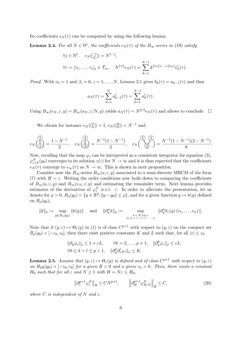
with the fully-discrete versions of the MRCMs obtained in Section (3) over η−2 periods ofthe stiff springs (that is, for a time interval of length T = 2πη−1). We compute the errors inpositions and momenta by comparing the results with a “reference solution” computed veryaccurately using the Deuflhard method (see e.g. [16]) with a very small constant step size.In Figure 1, the global errors at time t = 2π for the components q1,1, q1,2, p1,1, p1,2 versus thenumber of evaluations of the map ϕµ (computed with a high accuracy) are displayed for the

101 102 103

10−9

10−6

10−3

101 102 103

10−9

10−6

10−3

101 102 103

10−9

10−6

10−3

101 102 103

10−9

10−6

10−3

error in q1,1

fnc evals

error in p1,1

fnc evals

error in q1,2

fnc evals

error in p1,2

fnc evals

Figure 1: Problem (26) with η = 2−12 and initial conditions (27). Errors of multi-revolutioncomposition methods at time t = 2π as functions of the number of evaluations of ϕµ (formany values of the parameter N). Methods of orders 1 (circles), 2 (stars), 4 (s = 3 withwhite squares), 4 (s = 4 with black squares).

16

100 101 102 103 104 10510−9

10−6

10−3

100

100 101 102 103 104 10510−9

10−6

10−3

100

100 101 102 103 104 10510−9

10−6

10−3

100

100 101 102 103 104 10510−9

10−6

10−3

100

Error in energy with η = 2−10

fnc evals

Error in energy with η = 2−12

fnc evals

Error in energy with η = 2−14

fnc evals

Error in energy with η = 2−16

fnc evals

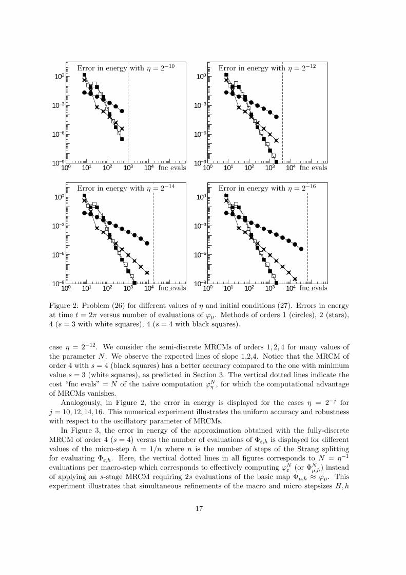
Figure 2: Problem (26) for different values of η and initial conditions (27). Errors in energyat time t = 2π versus number of evaluations of ϕµ. Methods of orders 1 (circles), 2 (stars),4 (s = 3 with white squares), 4 (s = 4 with black squares).

case η = 2−12. We consider the semi-discrete MRCMs of orders 1, 2, 4 for many values ofthe parameter N . We observe the expected lines of slope 1,2,4. Notice that the MRCM oforder 4 with s = 4 (black squares) has a better accuracy compared to the one with minimumvalue s = 3 (white squares), as predicted in Section 3. The vertical dotted lines indicate thecost “fnc evals” = N of the naive computation ϕN

η , for which the computational advantageof MRCMs vanishes.

Analogously, in Figure 2, the error in energy is displayed for the cases η = 2−j forj = 10, 12, 14, 16. This numerical experiment illustrates the uniform accuracy and robustnesswith respect to the oscillatory parameter of MRCMs.

In Figure 3, the error in energy of the approximation obtained with the fully-discreteMRCM of order 4 (s = 4) versus the number of evaluations of Φε,h is displayed for differentvalues of the micro-step h = 1/n where n is the number of steps of the Strang splittingfor evaluating Φε,h. Here, the vertical dotted lines in all figures corresponds to N = η−1

evaluations per macro-step which corresponds to effectively computing ϕNε (or ΦN

µ,h) insteadof applying an s-stage MRCM requiring 2s evaluations of the basic map Φµ,h ≈ ϕµ. Thisexperiment illustrates that simultaneous refinements of the macro and micro stepsizes H,h

17

is needed for fully-discrete MRCMs to converge, as predicted by Theorem 2.9.

101 102 103 10410−12

10−9

10−6

10−3

101 102 103 104

10−9

10−6

10−3

100Error in q1,2

fnc evals

Error in energy

fnc evals

Figure 3: Multi-revolution method of order 4 (s = 4) for the Hamiltonian (26) with η = 2−12.Error in energy in the multi-revolution approximation versus number of evaluations of Φε,h

approximating ϕε (final time t = 2π). The lines correspond respectively to h = 1/n =2−j−1, j = 1, . . . , 7 (from top to bottom).

Finally, in Figure 4, we plot, for η = 2−12, the evolutions of the stiff spring energies

Ik =1

2p22,k +

1

2η2q22,k, k = 1, 2, 3,

the adiabatic invariant I = I1 + I2 + I3 and the energy Eη(p, q) − 0.7 η on a time intervalof length T = 2πη−1 for η = 2−12. We observe excellent energy conservation and energyexchanges for the MRCM methods of orders 1, 2, 4 compared to the reference solution. Thisreference solution is computed with the standard Deuflhard method with constant step sizeh = η, totalizing about 1.1 · 108 steps (recall that a stepsize h comparable to the oscillatoryperiod is needed for standard highly oscillatory integrators). In comparison, notice thatthe total number of micro steps (Strang splitting) for each of the considered MRCMs is2snTη−1N−1 ≃ 1.0 · 106, which identical in all cases due to the chosen parameters N,n andthe stage number s of the MRCMs. What is striking in this experiment is that the multi-revolution composition approach yields errors in the energy exchanges lower than 5 percentsfor the methods of order 2 and 4 with a computational cost reduced by a factor 100 comparedto the standard reference integrator.

Remark 4.1. We have applied our MRCMs to the Hamiltonian Eη(p, q) in (26), by con-sidering for each value of η, a system of the form (10) that reduces to the original problemwhen ε = 2πη. This way, all the considerations made in the introduction for the applicationof MRCMs to systems of the form (10) apply directly to that case. Note that the consideredfamily of near-to-identity ϕε is different (although we do not reflect it in the notation) foreach particular value of η.

This is not however the only way to use MRCMs for the numerical integration of thatHamiltonian problem. For instance, the near-to-identity map ϕε could simply be defined as theflow with time 2πε of the Hamiltonian function Eε(p, q), in which case the convergence theoryin Section 2 would also apply. This approach may seem attractive because the map ϕε becomes

18

0 1 2.0

.5

1.0

1.5

0 1 2.0

.5

1.0

1.5

0 1 2.0

.5

1.0

1.5

0 1 2.0

.5

1.0

1.5

I2I3 I1

Eη − 0.7

I

time (×104)

reference solution

I2I3 I1

Eη − 0.7

I

time (×104)

MRCM of order 1 (N = 128, n = 8)

I2I3 I1

Eη − 0.7

I

time (×104)

MRCM of order 2 (N = 256, n = 8)

I2I3 I1

Eη − 0.7

I

time (×104)

MRCM of order 4 (N = 256, n = 4)

Figure 4: FPU-like problem (26) with η = 2−12. Energy exchanges on the time interval(0, 2πη−1). Multi-revolution methods of orders 1, 2, 4. Reference solution computed withconstant stepsize h = η by the standard Deuflhard method.

symmetric with respect to ε (i.e. ϕε ϕ−ε(y) = y) which would simplify considerably theorder conditions (similarly to the case of standard composition methods based on a symmetricbasic integrator). However, our numerical tests applied to (26) and similar to Fermi-Pasta-Ulam like problems indicate poor performances of the derived methods on time intervals ofsize O(ε−1). This seems to be related to the fact that the first order averaged ODE (3)corresponding to that particular choice of ϕε has unbounded solutions.

4.2 Application to the cubic nonlinear Schrodinger equation

Highly oscillatory problems of the form (10) are in particular obtained by appropriate dis-cretization in space of several Hamiltonian partial differentiation equations, such as nonlinearversions of wave equation and Schrodinger equation. In this section, we present some numer-ical experiments of the application of MRCMs to numerically integrate a problem consideredin [7] and originally analyzed by B. Grebert and C. Villegas-Blas in [15]. It consists of anonlinear Schrodinger equation in the with one-dimensional torus with a cubic nonlinearity|u|2u multiplied by an inciting term of the form 2 cos(2x),

i∂tu = −∆u+ 2ε cos(2x)|u|2u, t ≥ 0, u(t, ·) ∈ Hs(T2π) (28)

u(0, x) = cosx+ sinx.

19

0 1 2 3 4 5 610−9

10−6

10−3

100

0 1 2 3 4 5 610−9

10−6

10−3

100

0 1 2 3 4 5 610−9

10−6

10−3

100

0 1 2 3 4 5 610−9

10−6

10−3

100

time (×104)

reference solution (Strang splitting)

time (×104)

MRCM of order 2 (N = 100)

time (×104)

MRCM of order 2 (N = 20)

time (×104)

MRCM of order 4 (N = 100)

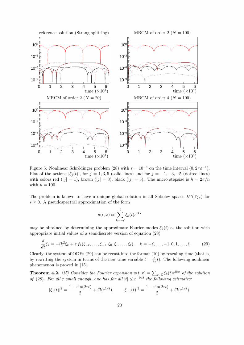
Figure 5: Nonlinear Schrodinger problem (28) with ε = 10−4 on the time interval (0, 2πε−1).Plot of the actions |ξj(t)|, for j = 1, 3, 5 (solid lines) and for j = −1,−3,−5 (dotted lines)with colors red (|j| = 1), brown (|j| = 3), black (|j| = 5). The micro stepsize is h = 2π/nwith n = 100.

The problem is known to have a unique global solution in all Sobolev spaces Hs(T2π) fors ≥ 0. A pseudospectral approximation of the form

u(t, x) ≈ℓ∑

k=−ℓ

ξk(t)eikx

may be obtained by determining the approximate Fourier modes ξk(t) as the solution withappropriate initial values of a semidiscrete version of equation (28)

d

dtξk = −ik2ξk + ε fk(ξ−ℓ, . . . , ξ−1, ξ0, ξ1, . . . , ξℓ), k = −ℓ, . . . ,−1, 0, 1, . . . , ℓ. (29)

Clearly, the system of ODEs (29) can be recast into the format (10) by rescaling time (that is,by rewriting the system in terms of the new time variable t = ε

2π t). The following nonlinearphenomenon is proved in [15].

Theorem 4.2. [15] Consider the Fourier expansion u(t, x) =∑

k∈Z ξk(t)eikx of the solution

of (28). For all ε small enough, one has for all |t| ≤ ε−9/8 the following estimates:

|ξ1(t)|2 =

1 + sin(2εt)

2+O(ε1/8), |ξ−1(t)|

2 =1− sin(2εt)

2+O(ε1/8).

20

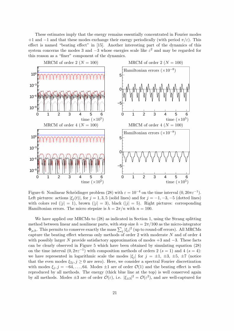
These estimates imply that the energy remains essentially concentrated in Fourier modes+1 and −1 and that these modes exchange their energy periodically (with period π/ε). Thiseffect is named “beating effect” in [15]. Another interesting part of the dynamics of thissystem concerns the modes 3 and −3 whose energies scale like ε2 and may be regarded forthis reason as a “finer” component of the dynamics.

0 1 2 3 4 5 610−9

10−6

10−3

100

0 1 2 3 4 5 6

−5

0

5

0 1 2 3 4 5 610−9

10−6

10−3

100

0 1 2 3 4 5 6

−5

0

5

time (×105)

MRCM of order 2 (N = 100)

time (×105)

Hamiltonian errors (×10−8)

MRCM of order 2 (N = 100)

time (×105)

MRCM of order 4 (N = 100)

time (×105)

Hamiltonian errors (×10−8)

MRCM of order 4 (N = 100)

Figure 6: Nonlinear Schrodinger problem (28) with ε = 10−4 on the time interval (0, 20πε−1).Left pictures: actions |ξj(t)|, for j = 1, 3, 5 (solid lines) and for j = −1,−3,−5 (dotted lines)with colors red (|j| = 1), brown (|j| = 3), black (|j| = 5). Right pictures: correspondingHamiltonian errors. The micro stepsize is h = 2π/n with n = 100.

We have applied our MRCMs to (28) as indicated in Section 1, using the Strang splittingmethod between linear and nonlinear parts, with step size h = 2π/100 as the micro-integratorΦµ,h. This permits to conserve exactly the mass

∑

j |ξj |2 (up to round-off errors). All MRCMs

capture the beating effect whereas only methods of order 2 with moderate N and of order 4with possibly larger N provide satisfactory approximation of modes +3 and −3. These factscan be clearly observed in Figure 5 which have been obtained by simulating equation (28)on the time interval (0, 2πε−1) with composition methods of orders 2 (s = 1) and 4 (s = 4):we have represented in logarithmic scale the modes |ξj | for j = ±1, ±3, ±5, ±7 (noticethat the even modes ξ2j , j ≥ 0 are zero). Here, we consider a spectral Fourier discretizationwith modes ξj , j = −64, . . . , 64. Modes ±1 are of order O(1) and the beating effect is well-reproduced by all methods. The energy (thick blue line at the top) is well conserved againby all methods. Modes ±3 are of order O(ε), i.e. |ξ±3|

2 = O(ε2), and are well-captured for

21

the second-order MRCM with moderate values of N or with the fourth-order MRCM withN = 100. Although we do not give here theoretical error estimates for PDEs, the qualitativebehavior of the dynamics of equation (28) is clearly well reproduced for a computational costthat is significantly smaller as compared to Strang splitting by its own. Here, for ε = 10−4,the cost is reduced by a factor 10 for the second-order MRCM and by a factor 16 for thefourth-order MRCM. In Figure 6, we further investigate the behavior of the methods ona time interval ten times larger. We observe that the beating effect is still well captured(left pictures, while an excellent energy conservation (without drift) can be observed (rightpictures).

5 Conclusion

We have presented a class of multi-revolution methods based on compositions for highlyoscillatory systems. We proved uniform convergence estimates independently of the stiffnessof the high oscillations which permits to use large time steps.

We point out that our convergence analysis applies only to bounded times intervals ofsize O(1) with respect to the ε. Notice however that, although to proposed schemes are notsymmetric (expect the symmetric method with s = 1 and the conjugate symmetric methodwith s = 2), the coefficients of the implemented methods are O(N−1) close to those of asymmetric method. This means that the excellent energy conservation results [16, Chap. 5]of symmetric methods applied to reversible systems remain valid for the proposed methodson longer time intervals of length T = O(ε−1).

The versatility and robustness of the multi-revolution approach is illustrated on variousproblems including the nonlinear Schrodinger equation. For the extension to infinite dimen-sional problems, we mention the recent works [8] in the context of the linear Schrodingerequation and [27] in the context of stochastic nonlinear systems.

References

[1] A. Abdulle, W. E, B. Engquist, and E. Vanden-Eijnden. The heterogeneous multiscale method.Acta Numer., 21:1–87, 2012.

[2] M. Calvo, L. O. Jay, J. I. Montijano, and L. Randez. Approximate compositions of a near identitymap by multi-revolution Runge-Kutta methods. Numer. Math., 97(4):635–666, 2004.

[3] M. Calvo, J. I. Montijano, and L. Randez. A family of explicit multirevolution Runge-Kuttamethods of order five. In Analytic and numerical techniques in orbital dynamics (Spanish) (Al-barracın, 2002), Monogr. Real Acad. Ci. Exact. Fıs.-Quım. Nat. Zaragoza, 22, pages 45–54. Acad.Cienc. Exact. Fıs. Quım. Nat. Zaragoza, Zaragoza, 2003.

[4] M. Calvo, J. I. Montijano, and L. Randez. On explicit multi-revolution Runge-Kutta schemes.Adv. Comput. Math., 26(1-3):105–120, 2007.

[5] M. P. Calvo, P. Chartier, A. Murua, and J. M. Sanz-Serna. Numerical stroboscopic averaging forODEs and DAEs. Appl. Numer. Math., 61(10):1077–1095, 2011.

[6] F. Castella, P. Chartier, S. Descombes, and G. Vilmart. Splitting methods with complex timesfor parabolic equations. BIT, 49(3):487–508, 2009.

[7] F. Castella, P. Chartier, F. Mehats, and A. Murua. Stroboscopic averaging for the nonlinearSchrodinger equation. Technical report, Sept. 2012.

22

[8] P. Chartier, F. Mehats, and M. Thalhammer. Convergence analysis of multi-revolution composi-tion time-splitting pseudo-spectral methods for Schrdinger equations. Part I. the linear case. Inpreparation, 2013.

[9] P. Chartier, A. Murua, and J. M. Sanz-Serna. Higher-order averaging, formal series and numericalintegration I: B-series. Found. Comput. Math., 10(6):695–727, 2010.

[10] P. Chartier, A. Murua, and J. M. Sanz-Serna. A formal series approach to averaging: exponen-tially small error estimates. Discrete Contin. Dyn. Syst., 32(9):3009–3027, 2012.

[11] W. E and B. Engquist. The heterogeneous multiscale methods. Commun. Math. Sci., 1(1):87–132,2003.

[12] W. E, B. Engquist, X. Li, W. Ren, and E. Vanden-Eijnden. Heterogeneous multiscale methods:a review. Commun. Comput. Phys., 2(3):367–450, 2007.

[13] E. Fermi, J. Pasta, and S. Ulam. Technical Report LA-1940, Los Alamos, 1955. Later publishedin E. Fermi: Collected Papers Chicago 1965 and Lect. Appl. Math. 15 143 1974.

[14] F. Filbet and S. Jin. A class of asymptotic-preserving schemes for kinetic equations and relatedproblems with stiff sources. J. Comput. Phys., 229(20):7625–7648, 2010.

[15] B. Grebert and C. Villegas-Blas. On the energy exchange between resonant modes in nonlinearSchrodinger equations. Ann. Inst. H. Poincare Anal. Non Lineaire, 28(1):127–134, 2011.

[16] E. Hairer, C. Lubich, and G. Wanner. Geometric numerical integration, volume 31 of Springer Se-ries in Computational Mathematics. Springer, Heidelberg, 2010. Structure-preserving algorithmsfor ordinary differential equations, Reprint of the second (2006) edition.

[17] E. Hansen and A. Ostermann. High order splitting methods for analytic semigroups exist. BIT,49(3):527–542, 2009.

[18] S. Jin. Efficient asymptotic-preserving (AP) schemes for some multiscale kinetic equations. SIAMJ. Sci. Comput., 21(2):441–454, 1999.

[19] U. Kirchgraber. An ODE-solver based on the method of averaging. Numer. Math., 53(6):621–652,1988.

[20] M. Lemou and L. Mieussens. A new asymptotic preserving scheme based on micro-macro formu-lation for linear kinetic equations in the diffusion limit. SIAM J. Sci. Comput., 31(1):334–368,2008.

[21] R. I. McLachlan. On the numerical integration of ordinary differential equations by symmetriccomposition methods. SIAM J. Sci. Comput., 16:151–168, 1995.

[22] R. I. McLachlan and G. R. W. Quispel. Splitting methods. Acta Numerica, 11:341–434, 2002.

[23] B. Melendo and M. Palacios. A new approach to the construction of multirevolution methodsand their implementation. Appl. Numer. Math., 23(2):259–274, 1997.

[24] A. Murua and J. M. Sanz-Serna. Order conditions for numerical integrators obtained by com-posing simpler integrators. Philos. Trans. Royal Soc. London ser. A, 357:1079–1100, 1999.

[25] L. R. Petzold, L. O. Jay, and J. Yen. Numerical solution of highly oscillatory ordinary differentialequations. In Acta numerica, 1997, volume 6 of Acta Numer., pages 437–483. Cambridge Univ.Press, Cambridge, 1997.

[26] J. Sanders, F. Verhulst, and J. Murdock. Averaging methods in nonlinear dynamical systems.Springer, New York, second edition, 2007.

[27] G. Vilmart. Weak second order multi-revolution composition methods for highly oscillatorystochastic differential equations with additive or multiplicative noise. Submitted, 2013.

23