Page 1
Multi-Robot Frontier Based Map Coverage Using the ROS Environment
by
Brian Pappas
A thesis submitted to the Graduate Faculty ofAuburn University
in partial fulfillment of therequirements for the Degree of
Master of Science
Auburn, AlabamaMay 4, 2014
Keywords: Collaborative robotics, Map coverage, Frontier navigation, Frontier detection
Copyright 2014 by Brian Pappas
Approved by
Thaddeus Roppel, Chair, Associate Professor of Electrical and Computer EngineeringPrathima Agrawal, Ginn Distinguished Professor of Electrical and Computer Engineering
John Hung, Professor of Electrical and Computer Engineering
Page 2
Abstract
Cooperative robotics deals with multiple robot platforms working to accomplish a com-
mon goal and has a multitude of applications including security, surveying, search and rescue,
and many more. The use of multiple robots allows a task to be completed more efficiently,
and is less prone to failure in the event that one of the robots becomes immobile.
The Robotic Operating System (ROS) is a mainstream software framework being used
for robotic research around the world. Despite its popularity and the very strong robotic
community behind its success, there has not been much work with ROS involving multi-
robot teams. This thesis presents a complete multi-robot system implemented within the
ROS software framework. Specifically, this work implements a collaborative robotic system
that performs map coverage of a known environment.
A team of robots is designed and programmed to cover a map with their range sensors.
A list of frontiers that border searched and unsearched space is maintained. Each robot is
assigned to travel towards unsearched space until the entire map has been covered.
The frontier-based coverage method is evaluated through a series of simulation experi-
ments in which the coverage planner is tested in different map environments while varying
the number of robots in the system. The ROS-based implementation of multi-robot frontier
coverage is shown to successfully be able to cover an entire area with a team of autonomous
robots.
ii
Page 3
Acknowledgments
I would first and foremost like to thank my advisor Dr. Thaddeus Roppel for his support
and guidance during my time at Auburn University. Dr Roppel gave me the opportunity to
become involved with robotics in the CRRLAB as an undergraduate student and provided
the freedom to explore my own research interests as a graduate student. He has served me
as an advisor, professor, mentor, and friend. I would like to thank Dr. Prathima Agrawal
for serving on my thesis committee and providing financial support for the lab enabling me
to take part and present at various conferences. I would also like to extend my gratitude to
Dr. John Hung for his time and support as a member of my thesis committee.
A very sincere thank you goes to my parents and sister for their words of encouragement,
willingness to listen (even when they had no idea what I was talking about), and constant
support throughout my life.
And finally I would like to extend thanks to all of my friends, both past and present.
You have been an integral part in helping me achieve my goals.
iii
Page 4
Table of Contents
Abstract . . . . . . . . . . . . . . . . . . . . . . . . . . . . . . . . . . . . . . . . . . . ii
Acknowledgments . . . . . . . . . . . . . . . . . . . . . . . . . . . . . . . . . . . . . . iii
List of Figures . . . . . . . . . . . . . . . . . . . . . . . . . . . . . . . . . . . . . . . vii
List of Tables . . . . . . . . . . . . . . . . . . . . . . . . . . . . . . . . . . . . . . . . ix
List of Abbreviations . . . . . . . . . . . . . . . . . . . . . . . . . . . . . . . . . . . . x
1 Introduction . . . . . . . . . . . . . . . . . . . . . . . . . . . . . . . . . . . . . . 1
1.1 Goals . . . . . . . . . . . . . . . . . . . . . . . . . . . . . . . . . . . . . . . . 2
1.2 Motivation . . . . . . . . . . . . . . . . . . . . . . . . . . . . . . . . . . . . . 3
2 Literature Survey . . . . . . . . . . . . . . . . . . . . . . . . . . . . . . . . . . . 5
2.1 Autonomous Mobile Robots . . . . . . . . . . . . . . . . . . . . . . . . . . . 5
2.2 Exploration and Coverage . . . . . . . . . . . . . . . . . . . . . . . . . . . . 6
2.3 Multi-Robot Coverage Strategies . . . . . . . . . . . . . . . . . . . . . . . . 6
2.3.1 Potential Methods . . . . . . . . . . . . . . . . . . . . . . . . . . . . 7
2.3.2 Graph Methods . . . . . . . . . . . . . . . . . . . . . . . . . . . . . . 7
2.3.3 Frontier Methods . . . . . . . . . . . . . . . . . . . . . . . . . . . . . 8
2.4 Summary . . . . . . . . . . . . . . . . . . . . . . . . . . . . . . . . . . . . . 9
3 Robotic Operating System . . . . . . . . . . . . . . . . . . . . . . . . . . . . . . 10
3.1 ROS Overview . . . . . . . . . . . . . . . . . . . . . . . . . . . . . . . . . . 10
3.2 Software Framework . . . . . . . . . . . . . . . . . . . . . . . . . . . . . . . 11
3.3 ROS Communcation . . . . . . . . . . . . . . . . . . . . . . . . . . . . . . . 12
3.3.1 Nodes . . . . . . . . . . . . . . . . . . . . . . . . . . . . . . . . . . . 12
3.3.2 Messages . . . . . . . . . . . . . . . . . . . . . . . . . . . . . . . . . . 12
3.3.3 Topics . . . . . . . . . . . . . . . . . . . . . . . . . . . . . . . . . . . 13
iv
Page 5
3.3.4 Services . . . . . . . . . . . . . . . . . . . . . . . . . . . . . . . . . . 14
3.3.5 Parameters . . . . . . . . . . . . . . . . . . . . . . . . . . . . . . . . 14
3.3.6 Distributed ROS . . . . . . . . . . . . . . . . . . . . . . . . . . . . . 15
3.4 ROS Navigation Stack . . . . . . . . . . . . . . . . . . . . . . . . . . . . . . 15
3.4.1 Localization . . . . . . . . . . . . . . . . . . . . . . . . . . . . . . . . 15
3.4.2 Path Planning . . . . . . . . . . . . . . . . . . . . . . . . . . . . . . . 16
3.5 Stage Simulator . . . . . . . . . . . . . . . . . . . . . . . . . . . . . . . . . . 17
3.5.1 World File . . . . . . . . . . . . . . . . . . . . . . . . . . . . . . . . . 17
3.5.2 Stage and ROS . . . . . . . . . . . . . . . . . . . . . . . . . . . . . . 18
4 Robot Hardware . . . . . . . . . . . . . . . . . . . . . . . . . . . . . . . . . . . 19
4.1 Chassis . . . . . . . . . . . . . . . . . . . . . . . . . . . . . . . . . . . . . . . 19
4.2 Power . . . . . . . . . . . . . . . . . . . . . . . . . . . . . . . . . . . . . . . 19
4.3 Drive System . . . . . . . . . . . . . . . . . . . . . . . . . . . . . . . . . . . 20
4.4 Range Sensors . . . . . . . . . . . . . . . . . . . . . . . . . . . . . . . . . . . 21
4.4.1 Kinect Sensor . . . . . . . . . . . . . . . . . . . . . . . . . . . . . . . 21
4.4.2 Hokuyo Lidar . . . . . . . . . . . . . . . . . . . . . . . . . . . . . . . 22
4.5 Control System . . . . . . . . . . . . . . . . . . . . . . . . . . . . . . . . . . 22
5 ROS Frontier Coverage Implementation . . . . . . . . . . . . . . . . . . . . . . . 24
5.1 Assumptions . . . . . . . . . . . . . . . . . . . . . . . . . . . . . . . . . . . . 24
5.2 Coverage Algorithm . . . . . . . . . . . . . . . . . . . . . . . . . . . . . . . . 25
5.2.1 Update Searched Space . . . . . . . . . . . . . . . . . . . . . . . . . . 26
5.2.2 Combine Searched Space . . . . . . . . . . . . . . . . . . . . . . . . . 28
5.2.3 Identify Frontiers . . . . . . . . . . . . . . . . . . . . . . . . . . . . . 29
5.2.4 Assign Frontiers . . . . . . . . . . . . . . . . . . . . . . . . . . . . . . 32
5.2.5 Support Nodes . . . . . . . . . . . . . . . . . . . . . . . . . . . . . . 34
5.3 Communcation Schemes . . . . . . . . . . . . . . . . . . . . . . . . . . . . . 34
5.3.1 Fully Distributed . . . . . . . . . . . . . . . . . . . . . . . . . . . . . 34
v
Page 6
5.3.2 Centralized Coordinator . . . . . . . . . . . . . . . . . . . . . . . . . 35
6 Experimental Setup and Results . . . . . . . . . . . . . . . . . . . . . . . . . . . 36
6.1 System Setup . . . . . . . . . . . . . . . . . . . . . . . . . . . . . . . . . . . 36
6.2 Coverage Results . . . . . . . . . . . . . . . . . . . . . . . . . . . . . . . . . 37
6.2.1 Broun Hall Map . . . . . . . . . . . . . . . . . . . . . . . . . . . . . . 38
6.2.2 Star Hall Map . . . . . . . . . . . . . . . . . . . . . . . . . . . . . . . 39
6.2.3 Office Map . . . . . . . . . . . . . . . . . . . . . . . . . . . . . . . . . 41
6.3 Nearest Frontier vs Rank Based Approach . . . . . . . . . . . . . . . . . . . 42
7 Conclusion and Future Work . . . . . . . . . . . . . . . . . . . . . . . . . . . . . 46
7.1 Summary . . . . . . . . . . . . . . . . . . . . . . . . . . . . . . . . . . . . . 46
7.2 Future Work . . . . . . . . . . . . . . . . . . . . . . . . . . . . . . . . . . . . 47
Appendices . . . . . . . . . . . . . . . . . . . . . . . . . . . . . . . . . . . . . . . . . 51
A ROS Node Interfaces . . . . . . . . . . . . . . . . . . . . . . . . . . . . . . . . . 52
B Encoder Divider Circuit . . . . . . . . . . . . . . . . . . . . . . . . . . . . . . . 54
vi
Page 7
List of Figures
3.1 ROS file system . . . . . . . . . . . . . . . . . . . . . . . . . . . . . . . . . . . . 12
3.2 ROS message definitions . . . . . . . . . . . . . . . . . . . . . . . . . . . . . . . 13
3.3 Relationship between nodes and topics . . . . . . . . . . . . . . . . . . . . . . . 14
3.4 Stage simulator GUI . . . . . . . . . . . . . . . . . . . . . . . . . . . . . . . . . 18
4.1 Test robot platform . . . . . . . . . . . . . . . . . . . . . . . . . . . . . . . . . 20
4.2 CRRLAB autonomous mobile robot team . . . . . . . . . . . . . . . . . . . . . 22
5.1 Phases for multi-robot coverage . . . . . . . . . . . . . . . . . . . . . . . . . . . 26
5.2 Sensor parameter combinations . . . . . . . . . . . . . . . . . . . . . . . . . . . 27
5.3 Results from combining robot searched areas . . . . . . . . . . . . . . . . . . . . 28
5.4 Image processing pipeline . . . . . . . . . . . . . . . . . . . . . . . . . . . . . . 29
5.5 Illustration of the frontier detection process . . . . . . . . . . . . . . . . . . . . 31
5.6 Frontier assignment differences . . . . . . . . . . . . . . . . . . . . . . . . . . . 33
6.1 Maps used for coverage experiments. Dimensions: 40m x 65.5m . . . . . . . . . 37
6.2 Coverage time vs number of robots for Broun Hall map . . . . . . . . . . . . . . 39
6.3 Coverage time vs number of robots for the Star Hall map . . . . . . . . . . . . . 40
vii
Page 8
6.4 Coverage time vs number of robots for the Office map . . . . . . . . . . . . . . 42
6.5 Coverage time comparison between nearest frontier approach and rank based
approach . . . . . . . . . . . . . . . . . . . . . . . . . . . . . . . . . . . . . . . 44
6.6 Robot coverage trajectories for rank based and nearest frontier approaches . . . 45
A.1 Node diagram legend . . . . . . . . . . . . . . . . . . . . . . . . . . . . . . . . . 52
A.2 robotSearched.py node interface . . . . . . . . . . . . . . . . . . . . . . . . . . . 52
A.3 combineSearch.py node interface . . . . . . . . . . . . . . . . . . . . . . . . . . 53
A.4 findFrontiers.py node interface . . . . . . . . . . . . . . . . . . . . . . . . . . . . 53
A.5 frontierPlanner.py node interface . . . . . . . . . . . . . . . . . . . . . . . . . . 53
B.1 Encoder divider circuit schematic . . . . . . . . . . . . . . . . . . . . . . . . . . 55
viii
Page 9
List of Tables
6.1 Coverage time (seconds) to completely cover Broun Hall with 1-6 robots . . . . 38
6.2 Coverage time (seconds) to completely cover the Star Hall map with 1-6 robots 40
6.3 Coverage time (seconds) to completely cover the Office map with 1-6 robots . . 41
B.1 Encoder circuit inputs . . . . . . . . . . . . . . . . . . . . . . . . . . . . . . . . 54
B.2 Encoder circuit outputs . . . . . . . . . . . . . . . . . . . . . . . . . . . . . . . 54
ix
Page 10
List of Abbreviations
AMCL Adaptive Monte-Carlo Localization
AMR Autonomous Mobile Robot
BBC British Broadcasting Cooperation
CRRLAB Cooperative Robotics Research Lab
FOV Field of View
GUI Graphical User Interface
LIDAR Light Detection and Ranging
LOS Line of Sight
PID Proportional, Integral, Derivative Control
ROS Robot Operating System
RVIZ Robot Visualization Tool
SLAM Simultaneous Location and Mapping
WFD Wave Front Detection
x
Page 11
Chapter 1
Introduction
In 1997, BBC’s popular science program “Tomorrow’s World” presented the first com-
mercially available autonomous vacuum cleaner, dubbed the Electrolux Trilobrite. The
Trilobrite was completely autonomous and only required the user to push a single but-
ton before it navigated itself around the futuristic home and cleaned dirty-floors on its own
[1]. Since the introduction of the Trilborite, many other companies, such as iRobot with
their Roomba vacuum, have entered the market with unyielding success. As of August 2012,
iRobot has reported selling more than 8 million fully autonomous cleaning robots worldwide,
proving that autonomous mobile robots are here to stay [2]. Even with all of the success,
robotic vacuum cleaners are only the tip of the iceberg for what autonomous mobile robots
are capable of doing.
Most of the research dealing with autonomous robots is focused on applications that
are too monotonous or too dangerous for humans to want to do themselves. Auburn Univer-
sity students built a sophisticated autonomous lawnmower capable of cutting around fences
and avoiding moving obstacles such as small animals [3]. Liquid Robotics has designed and
manufactured seafaring robots capable of autonomously exploring and gathering various data
about our planet‘s oceans [4]. One of the most important applications for autonomous robots
is search and rescue. According to FEMA, the time immediately following any disaster is the
most crucial time to provide aid to those who need it the most, however, it is also the time
period in which it is the most difficult to find such victims [5]. These are all prime examples
of uses where researchers want autonomous robots to be able to benefit our society in the
near future.
1
Page 12
All of the tasks mentioned thus far have several similarities that have become the focus
for many researchers in the field of robotics. First, they are all derivatives of the coverage
problem. The main principle behind the coverage problem is to completely cover the area
of a given environment with some type of sensor or end effector. For example, the goal of a
vacuum robot is to completely clean a given room with its motorized brush. Similarly one
of the goals of search and rescue is to find survivors in need by covering a given environment
with a sensor package capable of seeing or detecting humans. Since the coverage problem can
be time sensitive, the main evaluation metric for a solution is the amount of time required
to successfully cover an entire environment.
Second, all of the aforementioned tasks also benefit from scaling up the number of
robotic agents in use. The foremost idea is that these tasks can be completed in a more
time efficient manner if multiple collaborating robots are used instead of a single robot.
This is especially the case in any search and rescue operation where time can literally be the
difference between life and death. However, the addition of multiple robots working toward a
single goal does not come without difficulties. Collaborating robots have to communicate and
coordinate their actions in real time, and as more robots are added to a task, the complexity
of communication and coordination increases rapidly.
1.1 Goals
The work presented in this thesis aims to develop and implement a multi-robot frontier
based coverage system fully integrated into the Robot Operating System (ROS) framework.
In such a system, a team of identical autonomous robots equipped with laser range sensors
(LIDAR) autonomously deploy and cover a given two-dimensional map such that the LI-
DAR sensors detect all of the known open-space, effectively searching a given region. This
is completed by defining boundaries between searched space and unsearched space, which
are referred to as frontiers. The robots are required to share their current locations and
2
Page 13
previously searched areas with each other, while also coordinating which frontiers will be
explored by each robot in order to minimize total coverage time.
1.2 Motivation
ROS is an open source robotics framework created to ease the entry development hurdle
of robotic research by providing reusable software for common robotic subsystems, as well
as offering interfaces between high and low level functions. While still being relatively new,
since its release in 2009, ROS users have grown into a worldwide robotics community with
some of the most influential researchers utilizing ROS for state of the art robotics projects
[6].
One of the research and development areas that is lacking in the ROS community
is support for multi-robot systems. While ROS has thousands of software packages that
provide many types of robot functionality, from sensor integration all the way to complete
autonomous mapping, there are very few available implementations of successful multi-robot
systems. Therefore, the overall goal of this thesis is to add to the multi-robot functionality
of ROS by implementing a multi-robot frontier based navigation approach to the coverage
problem.
This objective involves many common tasks such as sensor integration, robot localiza-
tion, and robot navigation. Many of these tasks are already implemented within the ROS
environment and are heavily utilized, where applicable, in the development of the multi-
robot system. In addition, it is assumed a full and complete map of the environment to be
covered has previously been created and is available to all of the robots. Additionally it is
expected that all of the robots know their starting location within the environment. Due to
limited hardware the main analysis is performed in simulation using the Stage multi-robot
simulator [7] with a proof of concept trial implemented on physical mobile robot platforms.
The remainder of this thesis is organized in the following manner: Chapter 2 provides
an overview of the field of autonomous mobile robots with a focus on cooperative robotic
3
Page 14
coverage strategies. Chapter 3 gives a ROS primer and discusses the basic software topology
followed by the hardware used for the robots, which is presented in Chapter 4. Chapter 5
details the ROS implementation of the robot control system and the multi-robot coverage
algorithm. Chapter 6 presents the simulated experimental results, followed by the conclusion
and suggestions for future work in chapter 7.
4
Page 15
Chapter 2
Literature Survey
Since Asimov first coined the term “robotics” in his 1941 science fiction story “Liar!”,
the field of robotics has become a vast and multidisciplinary thrust in research institutions
around the world. The areas of robotic research in the second half of the twentieth century
have covered a breadth of topics including socially assistive robots [8], personal home au-
tomation robots [9], industrial manufacturing robots [10], search and rescue robots [11], and
many more. One of the significant branches in the robotics field is multi-agent systems, or
cooperative robotics. In a cooperative robotic system, a team of two or more mobile robotic
platforms is used to carry out a single task in an effort to complete that task in a more
effective manner over a single robot. This chapter introduces some key research concepts
relating to robotics with an emphasis on cooperative coverage of a given environment.
2.1 Autonomous Mobile Robots
Autonomous Mobile Robots (AMRs) are distinguished from remote control, or tele-
operated, mobile robots in the fact that there is no human in the loop controlling a robots
next action. In other words, the robot must be able to make decisions and execute its
choices all by computerized control. The following rules given in [12] summarizes the main
capabilities an AMR must possess over other types of robots. An AMR must be able to:
1. Gain information about the operation environment
2. Work for an extended period of time without human intervention
3. Move itself throughout its operating environment without human assistance
5
Page 16
4. Avoid situations that are harmful to people, property, or itself unless those are part of
its design specifications
2.2 Exploration and Coverage
One of the main applications in which teams of cooperative AMRs are being utilized is
to autonomously explore known environments [13]. Complete exploration of a known envi-
ronment is called coverage since the main idea is for a robot’s exteroceptive sensor system
to completely cover, or sweep, a given region. Coverage provides a challenge for autonomous
robots because the operation environment can be dynamically changing, especially if oper-
ating in close proximity to humans. Furthermore, cooperative robotics must take in account
the inherent need to communicate with one another which may place further constraints,
such as LOS (Line of Sight), on movement.
Robots that are designed for the autonomous coverage task must have robust sub-
systems capable of localizing a robot within its operating environment and successfully nav-
igating while avoiding boundaries and dynamic obstacles. Siegwart and Nourbakhsh present
an overview of many of the common methods for localization and navigation [14], and while
they are crucial to cooperative robotic systems, individual methods are not the focus for this
thesis.
2.3 Multi-Robot Coverage Strategies
Most of the literature for robot path planning considers the problem of navigation from
a start position to a goal position and there are many robust solutions to this problem
[15],[16],[17]. While the start-goal problem can be a sub-problem of multi-robot coverage,
it does not take into account coverage path planning requiring a sensor sweep of an entire
region. The goal of multi-robot coverage strategies is to minimize the amount time required
for the sensor sweep of the entire environment to be completed. There are many different
6
Page 17
specific approaches to coverage and this section outlines some of the more popular existing
approaches.
2.3.1 Potential Methods
Potential fields are a common approach to path finding due to their intuitive nature
and ease of implementation. Potential navigation methods require a robot to simply follow
a gradient descent in a fine grain two-dimensional grid representation of the map. In [18]
Howard et al propose a multi-robot coverage deployment scheme in which robots continuously
repel one another, analogous to the inverse square law of electrostatic potentials, until an
equilibrium state is reached. The approach requires many identical swarm like robots (on
the order of 100 nodes) that deploy over the search area. The method does not guarantee
complete coverage, as there may not be enough robots to completely cover the map once the
equilibrium state is reached.
This drawback can be solved by using overlapping potential fields to dynamically repel
the robots from obstacles and other agents, while attracting them to unsearched space;
however, this introduces local minima in the potential fields [19]. These local minima can
lead to trapped robots and ultimately a gridlock condition where all of the agents are trapped
in local minima and unable to move. Techniques do exist to detect and avoid local minima
[20], but are usually hybrid techniques of potential fields and other more complex coverage
methods.
2.3.2 Graph Methods
Graph based methods are another popular approach to the robot coverage problem. In
graph based methods the map is represented with a tree or graph like structure consisting of
edges and nodes. In this approach, the edges represent contiguous hallways while the nodes
represent intersections or decision points. This effectively transforms the coverage problem
into a graph traversal problem [21]. In [22], a branching spanning tree coverage method is
7
Page 18
introduced in which an optimal coverage plan is computed off-line before an experiment
begins.
In [23], the multi-robot coverage problem is transformed into the traditional graph
theory problem of the traveling salesman. The environment is divided into a graph of nodes
consisting of overlapping circles. The circles are placed in such a manner that if a robot
visits the center of every circle, the map will be covered. A genetic algorithm is then used to
determine optimal paths in order for every node to be visited in the least amount of time.
The main advantage of graph based nodes is that off-line pre-planning allows for optimal
routes to be calculated but would require complete re-planning, and the necessary commu-
nication infrastructure to go with it, should one of the robotic agents fail during execution.
While the optimal coverage path can be successfully computed, these methods are typically
not very robust as it cannot respond to failures or easily adapt to unknown obstacles within
a map.
2.3.3 Frontier Methods
The most common form of multi-robot coverage uses the concept of frontiers on the
boundaries of searched and unsearched space. The map is represented as an occupancy
grid where each cell represents free, occupied, or unknown space [24]. In [25], Rogers et
al uses a centralized coordination strategy for dispatching robots to frontiers. There is a
master coordinator node responsible for integrating all of the individual local robot search
spaces and directing each agent in real time to the nearest unclaimed frontier using a greedy
assignment strategy. This approach requires full communication such that the coordinator
knows the state of all robots at all times, and assumes that the environment is blanketed
with reliable wireless coverage linking all robots with the master coordinator.
In [26], the author presents an approach dubbed “MinPos”. The previous greedy ap-
proach is expanded upon by taking into account a robots distance, or rank, relative to all
of the individual frontiers. Reasoning on the rank forces the robots to spread out more by
8
Page 19
reducing the amount of repeated coverage by multiple robots and results in a reduction of
the over all search time. Additionally, the implementation is fully distributed. The robots
each contain the full state of the system and are only required to share their locations with
one another by broadcasting over an ad-hoc network.
Separate from the exploration strategy, frontier algorithms also require an efficient
method for identifying and clustering frontier cells within the occupancy grid. Several works
including [27] and [28] use the Wavefront Frontier Detection Method (WFD) that is based on
a breadth-first search algorithm starting from all of the robot’s current locations and grow-
ing until unknown space is found. The WFD approach can be prohibitively costly, as the
entire map has to be scanned each time the frontiers are updated. Improvements to WFD
are presented in [REF FastFrontier] which speeds up frontier detection time considerably by
updating the frontiers based on the current frontier state and new LIDAR scans while not
having to fully search the entire map.
2.4 Summary
While several popular coverage strategies have been mentioned, many other hybrid
navigation strategies exist and it is impossible to cleanly divide all of them into potential,
graph, and frontier techniques. All of the strategies have tradeoffs between optimality,
calculation complexity, and communication requirements, so there is no best overall strategy
for the coverage problem. Each individual coverage application will have its own unique
requirements and constraints that will have to be considered when choosing a coverage
coordination strategy.
9
Page 20
Chapter 3
Robotic Operating System
The frontier navigation approach presented in Chapter 5 is implemented using the Stage
software simulator and the Robotic Operating System (ROS). The Stage simulator, which
can be downloaded at [29] is an open source software package used to simulate collaborative
robot teams and the interaction of the team within a defined environment. ROS, which can
be downloaded from [30], is also an open source software package that provides a software
framework to aid in the development of complex robotic applications. ROS is designed to
work with both physical robots and simulated robots. In this work, when simulations are
used, Stage takes the place of the physical robots that would normally be controlled through
ROS. This chapter will provide an overview of the ROS framework and the Stage simulator,
and it will show which capabilities are used by the provided implementation of frontier
navigation. The following information is based on the ROS Hydro distribution running on
the Ubuntu 12.04 operating system.
3.1 ROS Overview
In the past few decades, the field of robotics has exploded with new technologies and
rapid advancements making it extremely difficult for a new researcher to quickly get involved
in cutting edge robotics. Robotic software must cover a broad range of topics and expertise
from low-level embedded systems, for controlling the physical robot actuators, all the way
up to high-level tasks such as collaboration and reasoning. The many layers of computation
have to seamlessly be able to communicate and integrate with each other for a robotic system
to function successfully. Additionally, several tasks, such as mapping and navigation, are
common to many robotic applications, however due to limitless combinations of robotic
10
Page 21
hardware, code reuse for such tasks is very difficult. In order to help alleviate the common
challenges of robotics research, many frameworks have been created that provide common
services and structure for writing software. One of the more successful frameworks heavily
used by the robotics community is ROS.
3.2 Software Framework
When it comes to designing software for robotics, ROS promotes the divide and conquer
approach. In this design paradigm, the subsystems that make up a robot are separated
into independent processing nodes that are then loosely coupled with a message passing
system. The independent nature of these processing nodes supports code reuse and prevents
researchers from having to “re-invent the wheel” when designing new robots. For example,
in [31], a driver for ROS to interact with an Arduino (a popular easy to use micro-controller)
was created and shared with the ROS community. It was quickly adopted by many users
and led to the development of many custom mobile robot platforms including the team of
cooperative robots this thesis is focused around.
To further promote code reuse and to proliferate the ease of sharing software, ROS
defines a recommended file structure and software build system. If software designers follow
the provided framework when designing robotic software, then almost any other person
using ROS should easily be able to download the software and use it immediately in their
own system. The file system uses the concept of packages (similar to the UNIX operating
systems) as the fundamental building block of the ROS ecosystem. Figure 3.1 shows a typical
file structure used by a ROS enabled robot.
A package can contain anything form individual executable files, libraries, or configura-
tion files, but the idea is that a package is a standalone organizational unit. Each package
contains a package manifest (package.xml) file that is used to describe the package and keep
track of any dependencies on other packages it may rely on. ROS provides a multitude of
11
Page 22
Figure 3.1: ROS file system
tools that allow the user to efficiently work with the file system and more information can
be found in the ROS tutorials at http://wiki.ros.org/ROS/Tutorials.
3.3 ROS Communcation
The distributed nature of ROS gives rise to specific concepts that allow many indepen-
dent computational processes to interact with each other, and together create the overall
behavior of a robotic system. The communication structure of ROS is designed around the
concept of nodes, messages, topics, services, and parameters.
3.3.1 Nodes
The individual computational entities that make up a ROS robotic system are called
nodes. Nodes are simply a process that performs computation and are usually robotic
subsystems written in Python or C++. For instance, a single node may be responsible for
taking velocity commands and controlling the motors accordingly.
3.3.2 Messages
Nodes are linked together by passing messages over topics. A message is a typed data
structure, which can contain almost any kind of data. Messages can contain other nested
messages to represent more complex data types. While ROS provides many commonly
12
Page 23
defined messages, users can create their own message types through the use of a message
(.msg) file.
(a) Twist message file
(b) Vector message file
Figure 3.2: ROS message definitions
Figure 3.2 shows an example of the files that make up a nested message. For example,
the twist message is used to define the instantaneous velocity of a robot in any direction and
is made of two-nested vector messages named “linear” and “angular”. The vector message
then contains three float64 primitive values named “x”, “y”,and “z.” In total, there are six
float64 values that makeup the twist message, three for each of the two vectors.
3.3.3 Topics
Nodes pass messages between each other through the use of topics. Nodes can subscribe
to topics in order to receive messages and they can publish a message to a topic for other
nodes to access via subscribing. Topics are the pipelines that loosely connect nodes together
while messages are the actual data that flows over the topic pipelines. Figure 3 illustrates
the relationship between nodes, messages, and topics.
Figure 3.3 is a graph that has been auto generated by the rqt graph tool provided by
ROS. The rqt graph output shows how nodes and topics are connected in a ROS system.
13
Page 24
Figure 3.3: Relationship between nodes and topics
The ellipses such as /joy2twist and /mot con node are nodes while the lines that connect
the nodes such as /cmd vel and /drive msg represent the topics. This graph represents a
robotic system in which a user can tele-operate a robot using a joystick and the robot will
keep track of its location relative to where the robot was powered on.
3.3.4 Services
Another node communication paradigm used by ROS is a service. Where topics are
asynchronous, in the sense that nodes do not have to explicitly communicate with each
other to exchange information, services provide synchronous communication. Services act
in a call-response manner where one node requests that another node execute a one-time
computation and provide a response. This can be useful when the system needs to perform
a specific task that does not fit the always-broadcasting architecture of topics and messages.
3.3.5 Parameters
ROS uses a parameter server to store and share status variables and non-high perfor-
mance data that is accessible to all of the nodes. The parameter server may be used to store
information such as map dimensions and the number of robots that are actively connected
to the system. This type of data is typically needed by many nodes and is not expected to
update frequently.
14
Page 25
3.3.6 Distributed ROS
Nodes, messages, topics, and services provide a powerful and robust framework for
designing robotic software systems and as robots become more complex, a single computer
may not be sufficient to handle all of the tasks that one robot requires. For this reason, ROS
is fully distributed and can work effortlessly over multiple physical computers. Nodes can
be executed on a network of computers, but can still communicate with topics and services
directly through the ROS framework. This allows for client/server setups in which a master
computer can remotely control a robot or perform complex calculations on a more powerful
remote computer.
3.4 ROS Navigation Stack
Sense the primary goal of this work is to provide a successful implementation of multi-
robot frontier navigation for the ROS ecosystem; the system realization takes full advantage
of ROS packages already available. The ROS navigation stack [32] is used to provide the
Localization and Path Planning capabilities of the system.
3.4.1 Localization
The Localization method used by the navigation stack uses the Adaptive Monte-Carlo
Localization (AMCL) approach presented in [15] and [33]. AMCL is based on a weighted
particle system in which each particle represents an estimated pose of the robot and consists
of two phases of calculation. The prediction phase combines new iterative measurement data
[∆x,∆y,∆Θ] from the on-board encoders and gyro sensors with the current state [xk, yk, Θk]
to create a new set of estimated pose locations [xk+1, yk+1, Θk+1] using the following set of
update equations:
15
Page 26
xk+1
yk+1
Θk+1
=
xk +
√∆x2 + ∆y2 ∗ cos(Θk + ∆Θ)
yk +√
∆x2 + ∆y2 ∗ sin(Θk + ∆Θ)
Θk + ∆Θ
The measured change in state contains noise inherent from the robots sensors and re-
quires an update phase for correction. During the update phase, the LIDAR sensor is
sampled and is compared to the expected measurement for each particle location. Each
particle is then weighted with a probability distribution. This results in a dense cluster of
high probability particles centered on the robots true location. The prediction phase and
update phase are continuously repeated at a rate of 10HZ providing real time localization
estimation. The localization approach also includes automatic recovery behaviors. Should
the probability estimate fall below a certain threshold, the robots will attempt to re-localize
by performing a 360-degree in-place rotation. If after several attempts the robots fail to
determine its current position, it will cease movement and terminate the current goal. This
is a rare occurrence and only happens in extreme cases of sensor occlusion.
3.4.2 Path Planning
The planning method used in the navigation stack is a cost-map based approach using
the A* algorithm [34]. The cost-map is a 2-dimensional grid of cells that represents the map
and the location of known obstacles. Each cell in the grid can only be one of three values:
free, occupied, or unknown. At a high level, the path planning approach requires the current
pose of the robot and a goal location, then outputs velocity commands to the robot base in
order to drive towards the goal. This functionality is realized by utilizing a global planner
and a local planner. The global planner uses the A* algorithm to plan an optimal path from
the current location to the goal location. However, the path generated is only based on the
known map and does not take into account dynamic obstacles that the robot may encounter
along the path. The local planner is responsible for generating the velocity commands that
16
Page 27
will move the robot through its immediate vicinity trying to follow the global plan and avoid
obstacles at the same time. This is completed using the Dynamic Window Approach (DWA)
[35] in which the possible range of velocity commands is sampled and forward simulated in
time. The results of the forward simulations are compared with a cost function that has
tunable parameters based on distance from obstacles, progress towards goal, and proximity
of the global plan. The set of velocity commands that have the lowest cost is selected and
sent to the mobile robot base. The planner is run at a rate of 30Hz allowing the robot to
move towards a goal while safely avoiding dynamic obstacles.
3.5 Stage Simulator
Stage is a two-dimensional multi-robot simulator used for the development and testing of
multi-robot navigation systems. Stage provides models for robots, sensors, and environmen-
tal objects and can simulate the interaction between these models [7]. Unlike other popular
simulators, Stage does not strive to be a very high fidelity simulator modeling complex phys-
ical interactions. Instead, Stage aims to be lightweight and provide a “good enough” fidelity
model of many systems and individual robots at once. This allows for rapid prototyping of
multi-robot systems without having to invest in large amounts of robotic hardware. Stage
includes a GUI (Figure 3.4) for monitoring the status of the simulated robot and sensor
systems and allows for quick validation and testing of navigating algorithms by providing a
time multiplier in which simulations can be carried out faster then real-time.
3.5.1 World File
Any simulation in Stage is configured via the use of a “.world” file and a black and
white bitmap image to represent the map. Every aspect of the simulation environment is
described through models with different properties in the “.world” file. The “.world” file
defines the map size, map bitmap file, number of robots, types of sensors, etc.
17
Page 28
Figure 3.4: Stage simulator GUI
3.5.2 Stage and ROS
Stage ROS is a ROS package that fully integrates the Stage simulator into the ROS
ecosystem by allowing communication and control through the use of ROS topics [36].
Stage ROS subscribes to a /cmd vel topic for each robot described in the “.world” file allow-
ing linear and angular velocity drive commands being published from another ROS node to
control the simulated robots. Furthermore, for each robot, Stage ROS publishes an /odom
topic containing simulated odometry information and various sensor topics depending on
what type of sensors have been configured in the “.world” file. Since Stage ROS integrates
completely with ROS, it is effectively a drop in replacement for the physical robot hardware.
In this way the same frontier controller presented in Chapter 5 can be used to control real
or simulated robots with no change to the sensor/control interface.
18
Page 29
Chapter 4
Robot Hardware
A team of three identical autonomous mobile robots was used for the hardware-based
experiments presented in Chapter 6. These robots were custom built specifically for work
dealing with cooperative robotics in Auburn University’s CRRLAB. The robots are fully
integrated into the ROS architecture and contain various sensors and electronics allowing
them to explore the environment while avoiding dynamic obstacles.
4.1 Chassis
The chassis shown in Figure 4.1 is the REX-16D platform from Zagros Robotics, which
consists of two drive motors, two free rotating caster wheels, and three 14-inch diameter
plastic disks for electronics and payload. The three circular disks are stacked on top of
one another separated by spacers creating three distinct platforms. The lowest of the three
platforms holds the drive system electronics including an Arduino Mega micro-controller,
motor driver, gyroscope sensor, power distribution board, and the battery. The second tier
holds a range sensor and the top level holds an Acer netbook running ROS that acts as the
hub for all of the other on board electronics.
4.2 Power
All of the electronics, with the exception of the Arduino and the laptop, are powered
through a 12V rechargeable lead acid battery. The PD-101 power distribution board is used
to provide a regulated 5V rail to all of the embedded electronics.
The Arduino is powered over USB via the laptop battery in order to isolate its operation
from the rest of the circuitry. The Arduino is responsible for aggregating odometry sensor
19
Page 30
Figure 4.1: Test robot platform
data and providing control signals to the motor controller board. Isolating the Arduino
allows this crucial function to not be interrupted should the main power supply fail or the
battery have a low charge. Furthermore, the isolation allows the Arduino to detect power
failures and alert the laptop of such incidents.
4.3 Drive System
The motors are mounted horizontally opposed creating a differential drive system. The
motors can drive the platform up to 0.5 m/sec and includes an integrated quadrature hall-
effect encoder that generates over 32000 encoder pulses for one revolution of the main drive
20
Page 31
shaft. The castor wheels are placed on the front and rear of robot base to provide stability
for the platform.
The high resolution of the encoders initially resulted in the Arduino not being able
to process every single pulse, so a simple digital logic circuit was created to divided the
quadrature encoder signal by 16 resulting in approximately 2100 pulses for one revolution
of the drive shaft. The encoder circuit details are documented in Appendix B. Even though
this reduces the encoder resolution, the Arduino can easily handle the lower data rate and
2100 pulses per revolution is still more then enough resolution to provide accurate odometry
estimation. The odometry calculations also take advantage of a MEMS gyro sensor mounted
on the lowest level to measure rotation around the center of the robot along the vertical axis.
4.4 Range Sensors
The robots are outfitted with one of two possible range sensors to be used for navigation.
The range sensor is either the first generation XBOX KinectTM or the Hokuyo URG-04lx-
UGO1 scanning range finder.
4.4.1 Kinect Sensor
The XBOX KinectTM sensor is a gaming peripheral that usually accompanies the Mi-
crosfot XBOX 360 home entertainment system, however, it also makes an easy to use vi-
sion/range sensor. Due to its availability and low cost, the Kinect was the first choice of
sensor, however its limitations became quickly apparent.
Since the ranging technology is based off infrared light, only one Kinect could safely
operate at a time. This made multi-robot operations difficult since the multiple Kinects
would interfere with one another. The measured range data was accurate to within +/-
4cm for distances of 3m or less, but quickly grew noisy at longer distances. Furthermore,
the Kinect had a substantially narrower field of view (70-degrees) when compared to the
Hokuyo LIDAR (240-degrees) sensor.
21
Page 32
4.4.2 Hokuyo Lidar
The Hokuyo URG-04lx-UGO1 is a dedicated laser range finder (LIDAR) used in many
robot applications and with an accuracy +/-30mm at a 5.6 m range, it is well suited to the
mapping task. While the sensor has a 240-degree FOV, due to its mounting location on
the front of the robot, only the forward facing 180 degrees are used for range measurement
purposes. Typically LIDAR sensors are mounted on top of the robot to have the maximum
un-occluded FOV, but this would not allow the robots to be able to detect one another
as obstacles. The CRRLAB at Auburn University only has access to two LIDAR sensors,
therefore in experiments using three robot platforms, two robots are outfitted with the
LIDAR and one robot is outfitted with the XBOX Kinect.
Figure 4.2: CRRLAB autonomous mobile robot team
4.5 Control System
The drive system is controlled by a pair of PID feedback loops (one for each drive
wheel) run with an update interval of 100Hz. The motion controller, whether it be automatic
navigation or manual tele-operation, requests the robot base to drive at a specified linear and
angular velocity. The requested linear and angular velocities are transformed to individual
left and right wheel velocities using the following kinematic equations:
22
Page 33
Vl = −ΘL
2+R Vr =
ΘL
2+R
where Vl and Vr represent the respective left and right wheel velocities, θ is the angular
velocity, R is the linear velocity, and L is the wheel base diameter. The left wheel velocity
contains a negative because the angular velocity is chosen to be positive when the robot is
turning left.
The actual wheel velocities are estimated by measuring the number of encoder ticks
received for each measurement interval. The difference between the actual wheel velocities
and the requested wheel velocities is used as the error input for the PID controllers. The
PID gains were tuned by hand until the robot base closely followed the requested velocity
commands.
23
Page 34
Chapter 5
ROS Frontier Coverage Implementation
In order for a multi-robot coverage system to function properly, there are several sub-
problems that have to be solved. The system must be able to track areas already covered by
the robot’s sensors, detect frontiers between searched and unsearched space, assign frontiers
to individual robot platforms, and navigate the robots to their assigned frontier region.
Since ROS promotes the “divide and conquer” methodology to robot software design, these
sub-problems provide a convenient division for dividing the coverage problem into a set of
individual ROS nodes. Dividing the design into ROS nodes that perform specific subtasks
enables future modular development of the robot system. For example, if a different frontier
coverage algorithm is desired, the ROS nodes responsible for identifying frontiers can be
reused, and a new node that handles the task of frontier assignment can easily be dropped
into the system in a plug-and-play manner. This chapter outlines the operation of the multi-
robot frontier coverage algorithm and details how the system is implemented within the ROS
framework.
5.1 Assumptions
Multi-robot coverage can be implemented on a huge variety of robotic platforms with an
equally large variety of capabilities. The presented coverage implementation relies on several
operational assumptions to narrow the implementation goal to a specific scope. First, it is
assumed an occupancy grid representation of the static map is available to all robots. This
removes the requirement for multi-robot SLAM and map merging, which are outside the
scope of this thesis. Second, common to most coverage algorithms, each robot knows its
starting pose (position and orientation) within the two-dimensional map in order to prevent
24
Page 35
a lengthy pre-localization process. Third, the robots maintain an accurate estimation of
their pose within the occupancy grid map. Fourth, a wireless communication network is
available over the entire coverage region. If a robot loses communication with the network
it is considered a failed robot and will be unable to re-establish communication. Fifth, the
robot sensor that will sweep the environment is assumed to be static relative to the robot
base. This allows the coverage area of the robot to be determined by only knowing the
robot’s pose.
5.2 Coverage Algorithm
The complete multi-robot coverage approach is divided into six discrete phases that
each robot must be able to carry out on its own. Each robot must be able to:
1. Localize itself within the map
2. Continuously update the occupancy map grid cells that have been successfully searched
3. Combine the received searched maps from other robots into a single searched map
4. Identify frontiers
5. Assign robots to frontiers
6. Autonomously navigate towards the assigned frontier
These six phases are continuously run in a loop until the entire map area has been covered.
Phase 1 and phase 6 are functionality provided by existing ROS packages as explained in
Chapter 3. The other four phases, shown as orange in Figure 5.1, indicate the custom ROS
nodes that make up a single ROS package named gen2 frontier.
Each custom node is implemented in Python and the corresponding file name is listed
under the node in Figure 5.1. The computation details of each of each of these nodes are
further outlined below. Refer to Appendix A for the ROS interface used for each node.
25
Page 36
Localize Update Searched
Combine Searched
Iden6fy Fron6ers
Assign Fron6ers Navigate
Frontier Coverage Package (gen2_frontier)
Provided by ROS
Provided by ROS
robotSearched.py combineSearchSpace.py 2indFrontiers.py frontierPlanner.py
1 2 3 4 5 6
Figure 5.1: Phases for multi-robot coverage
5.2.1 Update Searched Space
The robotSearched.py node is responsible for creating and updating an occupancy grid
that represents the searched space and the unsearched space of the underlying map for one
individual robot. This node is run locally on each robot platform so that each robot is
responsible for tracking the regions it has searched individually. The node is designed to be
configurable to account for a wide range of sensor configurations allowing the user to change
the effective sensor scan area used for coverage. The node interface in Figure A.2 indicates
the ROS structure of the node.
The node subscribes to the /map topic and the /amcl pose topic which represent the
static obstacle occupancy map and the robots pose within the occupancy map respectively. A
new occupancy map is published on the robotSearched topic, however, instead of representing
known/unknown space, this new occupancy map indicates searched/unsearched space. The
published occupancy grid is persistent over update intervals, which allows the robot to log
all areas it has searched since an experiment began.
The shape of the search area is governed by three parameters passed to the node when
it is launched. The ∼senseType parameter selects the overall geometric shape of the sensor
area. The current possible shapes are “circle”,“semi-circle”, “square”, and “trapezoid” The
“circle” and “semi-circle” are useful for modeling LIDAR sensors while the “square” and
“trapezoid” options are more useful for modeling standard video cameras. The ∼senseDist
parameter is used to scale the range of the sensors and represents the maximum distance the
26
Page 37
robot can sense straight ahead. The ∼senseLOS parameter can take the value of “True” or
“False” and selects whether the sensor is limited to LOS (line of sight) constraints. When
set to “True,” the robots are not allowed to see through walls or obstacles. Figure 5.2 shows
the results of different parameter combinations.
(a) Circle LOS=“True” (b) Circle LOS=“False”
(c) Square LOS=“True” (d) Square LOS =‘False’
Figure 5.2: Sensor parameter combinations
The node also provides the /clearSearched service which allows all of the searched space
in the occupancy grid to be reset to unsearched space. This is provided as a convenience
service such that the node does not have to be shutdown and restarted between experiments.
27
Page 38
5.2.2 Combine Searched Space
The combineSearchSpace.py node (Figure A.3) aggregates the individual searched areas
of all robots into one occupancy grid and is the only node that requires data to be shared
amongst the robots. However, the node is not responsible for handling robot-robot commu-
nication directly as that is taken care of automatically by the ROS message passing system.
The node subscribes to each /robotSearched topic published by the individual robots and
requires the ∼numRobots parameter to be set to the active number of robots in the system
in order to know how many topic subscriptions should exist. Each searched area received
from the individual robots is overlaid on top of one another to create one occupancy grid
that represents all of the searched space for the entire robot team as illustrated in Figure
5.3.
(a) Robot 0 coverage (b) Robot 1 coverage
(c) Robot 2 coverage (d) Combined coverage
Figure 5.3: Results from combining robot searched areas
The node publishes the same information over two separate formats. The /searchedCom-
bine occupancy grid topic is used only for visualization in the RVIZ (Robot Visualization)
tool provided by ROS. The /searchedCombineImage topic is the same information stored in
an image format which is to be used for locating frontiers in the next phase.
28
Page 39
5.2.3 Identify Frontiers
The findFrontiers.py node (Figure A.4) subscribes to the original map occupancy grid on
the /map topic and the /searchedCombineImage topic published by the combineSearchSpace.py
node. From these two sources, the node publishes a set of map coordinates representing the
geometric centroid of each frontier on the /frontierMarker topic. An additional image is
published on the /frontierImage topic for visualization purposes only.
Two different computation methods were considered for identifying the frontiers be-
tween searched and unsearched space. The first, which is the typical approach found in
most literature, propagates a wavefront over the occupancy grid from each robot’s position,
stopping when unsearched space is reached. Adjacent frontier grid cells are clustered to-
gether to make a continuous frontier. Several wavefronts, one for each robot, would have
to propagate simultaneously leading to overlap conditions and an asynchronous ending time
for each wavefront. This method proved computationally costly and not practical for real
time systems when large maps and a large robot team was used.
The findFrontiers.py node breaks away from the occupancy grid map representation and
identifies frontier regions based on digital image processing techniques. A sequential image
processing pipeline, illustrated in Figure 5.4, utilizes the open source OpenCV libraries [37]
for all image processing.
Edge Detec)on
Edge Removal Filter
Dila)on Contour Detec)on
Contour Markers
1 2 3 4 5
Searched Combine
Map
Source Images
Figure 5.4: Image processing pipeline
29
Page 40
Edge Detection and Edge Removal
The first step in identifying the frontiers is to find all of the image pixels that are on the
boundary of searched and unsearched space through the use of edge detection on two source
images. The “Map” source image is a binary image representation of the map occupancy
grid in which black indicates freespace and white indicates occupied space (Figure 5.5a).
The “Combined Search” image is a ternary image in which white indicates free unsearched
space, black indicates free searched space, and gray indicates occupied space (Figure 5.5b).
A modified sobel edge detector is used to extract the edges without introducing any
Gaussian blur. Since the source images contain hard edges, in which the entire gradient
transition takes place on the edge of two adjacent pixels, perfect edge detection can be
achieved. A threshold is applied to the resulting pair of images outlining all edges in white
with the rest of the image black. The edges detected on the “Map” image (Figure 5.5c)
outline the map boundary while the edges detected on the “Searched Combine” image (Figure
5.5d) outline the map boundary and the frontier edges. Subtracting the image intensity
containing the map boundary from the image intensity containing the map boundary and
the frontier boundaries produces an image that only has the frontier pixels in white with the
rest of the image being black.
Dilation, Contour Detection, and Markers
The frontier pixels are dilated forming a set of contours or blobs in the image (Figure
5.5e). The location of each contour designates a discrete frontier region. A built in contour
detector provided by the OpenCV libraries is used to find the size of each contour and a
minimum size threshold is set to filter out any stray frontier pixels. The COG (center of
gravity) of each remaining contour is found and published on the /frontierImage topic as a
set of markers that can be visualized in RVIZ. Figure 5.5f shows the RVIZ visualization in
which the white is the searched space, black is the unsearched space, gray is obstacles, the
30
Page 41
blue circles represent the COG of each frontier, and the remaining circles are the current
robot locations.
(a) Map (b) Combined Searched (c) Map Edges
(d) Combined Searched Edges (e) Dilated Frontier Edges (f) RVIZ Visualization
Figure 5.5: Illustration of the frontier detection process
31
Page 42
5.2.4 Assign Frontiers
The frontierPlanner.py node (Figure A.5) subscribes to the marker message published
by the findFrontiers.py node and intelligently assigns each robot to a frontier marker. The
method used for the assignment of frontiers is an extension of the “MinPos” approach used
in [26]. Similar to a nearest frontier or greedy assignment method, this approach is based on
the distance to all possible frontiers of each robot, however, it also takes into account the
rank of each robot towards each frontier. The rank for any given robot and frontier pair is
calculated by counting the number of other robots that are closer to the frontier. In general,
a robot will be assigned to the frontier it is in the best position for, i.e. the frontier with the
lowest rank.
As long as the robots can accurately communicate their pose with one another, multiple
running instances of this node should always result in the same frontier assignments for each
robot. In this manner, each robot can locally run an instance of this node to create a fully
distributed system that does not require a master coordinator.
Assigning frontiers for exploration based on the rank causes the robots to spread out
more as illustrated in Figure 5.6a. Even though robot R3 is closer to frontiers F2, F3, and
F4, it is still assigned to frontier F1, as it is the closest robot to that particular frontier.
This is an improvement over the greedy approach, shown in Figure 5.6b, in which robot R3
is assigned to the nearest unassigned frontier resulting in robot R3 moving towards robots
R1 and R2 and through previously searched space to reach frontier F4. It is also a vast
improvement of the nearest frontier strategy depicted in 6.6b which results in both robot R3
and R1 heading towards the same frontier. The rank based approach spatially separates the
robots more effectively then the greedy or nearest based approaches.
Rank is determined through the use of a cost matrix C. Index Cij of the cost matrix
is the distance that robot Ri would have to travel to reach frontier Fj. The cost matrix
is populated by asking the ROS navigation stack to plan a global path from each robot to
each frontier. Given the cost matrix C, a position matrix P is created where the index Pij
32
Page 43
F1
1 2
3
F2 F3
F4
(a) Rank based
F1
1 2
3
F2 F3
F4
(b) Greedy based
F1
1 2
3
F2 F3
F4
(c) Nearest based
Figure 5.6: Frontier assignment differences
associates the rank of robot Ri towards frontier Fj. Given a set of robots R and the cost
matrix C, the position matrix index Pij can be defined as follows:
Pij =∑
∀Rk∈R,k 6=i,Ckj<Cij
1
Ideally each robot would be in the best position for exactly one frontier, however, this is
hardly the case. Any time a robot’s best rank is tied for more then one frontier, the frontier
33
Page 44
with the lowest cost is chosen. In Figure 5.6a robot R2 has a rank of “1” for frontiers F3
and F4, but it was assigned to frontier F3 as it incurs the lowest cost.
5.2.5 Support Nodes
The gen2 frontier package also includes two support nodes that are not directly related
to the frontier detection and navigation effort. The resetSearched.py node is a simple node
that calls the /clearSearched service in each active robot. This is used to rapidly reset the
system after a completed coverage run. The recordData.py monitors a running system and
records the total coverage time as well as the percentage of the map covered over time. The
data is stored to the disk and used for analyzing performance at a later time.
5.3 Communcation Schemes
The robots communicate over an 802.11g wi-fi network. Since ROS nodes themselves are
fully distributed over a networked computer system, there are several options for configuring
which nodes will run on which computers.
5.3.1 Fully Distributed
In a fully distributed setup, each robot will run one instance of each node in the
gen2 frontier package. In this configuration each robot will separately receive and combine
the searched maps from the other robots and then carry out all of the frontier assignment
calculations locally. Each robot should arrive at the same frontier assignment conclusions
and only needs to act upon the frontier that it has assigned itself. In the current implemen-
tation the fully distributed approach requires full and complete communication amongst all
of the robot platforms and should only be used if reliable wi-fi coverage is guaranteed.
34
Page 45
5.3.2 Centralized Coordinator
A centralized communication scheme relies on another computer acting as a coordinator
for the robots and is useful when the operation of the coverage system needs to be monitored
in real time. In this scheme, each robot runs an instance of the robot searched.py node
while the other three nodes of the gen2 frontier package are run on the coordinator. The
coordinator is then responsible for aggregating the searched space and assigning frontiers to
the robots. In the current implementation, the coordinator can detect a failed robot and
successfully remove it from the system allowing the remaining working robots to complete
the coverage task.
35
Page 46
Chapter 6
Experimental Setup and Results
The frontier coverage approach implemented in the gen2 frontier package was exten-
sively tested by varying the number of robots, the type of map environment, and other
simulation parameters in order to characterize the performance and behavior of the system.
The quantitative analysis is based on a complete simulated system. The simulation allows
quick evaluation with more robot platforms then physically exists, and also allows the un-
derlying coverage map to be changed without having to move the physical robots to a new
location.
6.1 System Setup
For the coverage results presented in section 6.2 the system was evaluated based on the
amount of time it took for a team of robots to completely cover all of the open space in a given
map. The robots were configured to have a circular 360-degree omni-directional coverage
sensor with a range of 6m from the center of the robot. Additionally, the ∼senseDist param-
eter from the robotSearched.py node was set to “True” which enabled the LOS constraints.
The robots would not be able to see through the walls.
Three different maps, shown in Figure 6.1 were used during the experiments. In each
map, the black area represents walls and obstalces, the white area represents the free space
that needs to be covered, and the gray area is space outside the map boundary. Each of
the rectangular regions that encloses a map in Figure 6.1 represents an area with a width of
40m and a height of 65.5m. Figure 6.1a is a map of the third floor of Broun Hall at Auburn
University and was automatically generated by one of the robot’s SLAM capabilities. The
map in Figure 6.1b is a fictional map with a large star shaped intersection that provides
36
Page 47
many possible options for a team of robots to spread out during coverage. The map in
Figure 6.1c represents a typical office like environment consisting of hallways and individual
rooms. This map was chosen to test the system in a more complex and realistic environment.
(a) Broun Hall Map (b) Star Hall Map (c) Office Map
Figure 6.1: Maps used for coverage experiments. Dimensions: 40m x 65.5m
6.2 Coverage Results
For each map in Figure 6.1 the number of robots was varied from 1 to 6. A minimum of
five simulation runs was executed for each map and number of robots combination. For each
experiment the robots began clustered together around a starting point that was randomly
placed somewhere on the map periphery in order to simulate all of the robots being deployed
by a user at the same time. While traversing a path to a frontier, each robot was commanded
to accelerate to its maximum velocity of 0.5m/s. All given durations represent simulated
real-time in seconds. The results of these simulations are summarized below.
37
Page 48
6.2.1 Broun Hall Map
The minimum, average, and maximum coverage times for each number of robots in
the Broun Hall map is shown in Table 6.1 and plotted in Figure 6.2. The Broun Hall
map is a relatively simple map that does not fully benefit from large numbers of robots as
there are very few intersections that allows the team to spread out. This is evident by a
maximum speedup of only 2.33 over a single robot during the five robot test. During the
experiments it was observed that the lack of navigation options resulted in groups of 2 or
more robots following one another. Robots that were forced to remain in close proximity
with one another would end up interfering with each other’s navigation planning leading
to less efficient coverage. When the the sixth robot was added, the average coverage time
actually increased due to an overcrowded map.
Table 6.1: Coverage time (seconds) to completely cover Broun Hall with 1-6 robots
# Robots Min Time Avg Time Max Time Avg. Speedup
1 290.8 319.4 350.1 N/A
2 172.0 187.7 205.9 1.70
3 170.0 177.8 185.7 1.79
4 108.1 144.7 178.2 2.21
5 132.5 137.3 148.3 2.33
6 133.6 142.7 152.5 2.24
The overall best coverage time of 108.1 seconds occurred with a team of four robots
which resulted in a speedup factor of 2.95 when compared to the average single robot run.
During this run, the robots were able to spread out in a near optimal manner where each
robot was able to continuously explore unsearched areas without overlapping another robot
or having to double back on searched space to reach an unsearched area.
38
Page 49
1 2 3 4 5 6100
150
200
250
300
350
400Coverage Time vs Number of Robots for the Broun Map
Number of Robots
Tim
e (s
ec)
Min TimeAverage TimeMax Time
Figure 6.2: Coverage time vs number of robots for Broun Hall map
6.2.2 Star Hall Map
The Star Hall map, characterized by the by the six-way star shaped intersection in the
center, is well suited for multi-robot coverage. The plethora of routing options and hallway
intersections allows multiple robots to spread out more effectively leading to significantly
higher speedup ratings for each number of robots when compared to the the Broun Hall
map. The minimum, average, and maximum coverage times for each number of robots in
the Star Hall map is shown in Table 6.2 and plotted in Figure 6.3.
The average search time monotonically decreases as each robot is added but at a di-
minished rate of return. The addition of the second, third, and fourth robots each led to
significant speedups with the speedup of four robots being 3.19. The addition of the fifth
39
Page 50
Table 6.2: Coverage time (seconds) to completely cover the Star Hall map with 1-6 robots
# Robots Min Time Avg Time Max Time Avg. Speedup
1 613.4 625.0 648.1 N/A
2 327.8 352.2 368.4 1.77
3 238.3 257.2 275.5 2.43
4 181.9 195.8 208.2 3.19
5 174.8 191.7 213.3 3.26
6 183.0 189.1 196.5 3.31
1 2 3 4 5 6150
200
250
300
350
400
450
500
550
600
650Coverage Time vs Number of Robots for the Star Map
Number of Robots
Tim
e (s
ec)
Min TimeAverage TimeMax Time
Figure 6.3: Coverage time vs number of robots for the Star Hall map
and sixth robots, however, only increased the speedup slightly from 3.19 with four robots to
3.31 with 6 robots. Even with a map more suited for multi-robot operations, the addition
of the sixth robot still led to overcrowding and robot interference. This is illustrated as the
40
Page 51
overall best coverage time for the Star Hall map was 174.8 seconds with 5 robots when it is
expected that 6 robots would provide the best coverage time.
6.2.3 Office Map
The Office map is the most complex environment out of the three maps used during
experiments. The previous maps focused mainly on hallway type environments, but the
Office map adds individual rooms. The sharp corners and concave spaces leads to the
existence of many more frontiers at any given point when compared with the previous two
maps. The additional number of frontiers creates a larger search-space when evaluating
the rank for each robot and frontier pair. This can have an adverse effect on performance
depending on the processing capabilities of the computer.
Table 6.3: Coverage time (seconds) to completely cover the Office map with 1-6 robots
# Robots Min Time Avg Time Max Time Avg. Speedup
1 1002.3 1054.0 1129.7 N/A
2 543.2 574.6 597.5 1.83
3 379.3 432.8 575.5 2.44
4 289.5 326.8 362.8 3.23
5 314.5 339.6 363.0 3.10
6 306.9 327.7 361.3 3.21
For one of the runs with 6 robots the maximum frontier count exceeded 15 individual
frontiers. In order to calculate the rank for each robot, a path from each robot to each
frontier must be generated which results in the planning of over 90 distinct paths. The rank
computation is repeated at a 1Hz rate and even with a modern day computer with an Intel
i7 processor, the path planning for the 6 robot experiment on the Office Map began to take
slightly longer then the 1Hz required rate. While this did not greatly impact the results, it
does indicate an upper bound constraint, determined by computer processing power, on the
type of map and number of robots that can be used with this rank based coverage approach.
41
Page 52
The simulation results follow the same trend of a diminishing return with increasing
number of robots. The speedup factor was not as great as the Star Map because the addition
of the individual rooms in the map made the robots have to constantly double back on
searched areas to reach a new frontier. The minimum, average, and maximum coverage
times for each number of robots in the Star Hall map is shown in Table 6.3 and plotted in
Figure 6.4.
1 2 3 4 5 6200
300
400
500
600
700
800
900
1000
1100
1200Coverage Time vs Number of Robots for the Office Map
Number of Robots
Tim
e (s
ec)
Min TimeAverage TimeMax Time
Figure 6.4: Coverage time vs number of robots for the Office map
6.3 Nearest Frontier vs Rank Based Approach
The purpose of choosing the rank based frontier coverage scheme was to force the robots
to spread out more effectively and ultimately cover the map in an efficient manner. In order
42
Page 53
to evaluate the effectiveness, the rank based coverage scheme was compared with the nearest
frontier approach. For this experiment, the frontierPlanne.py node was temporarily modified
such that robots would always be assigned to their nearest frontier regardless of rank. The
comparison was carried out on the Star Hall map while varying the number of robot from 1
to 6. The coverage times are shown in Figure 6.5 with the nearest frontier approach in blue
and the rank based approach in green.
For two or more robots, the rank based approach consistently outperformed the nearest
frontier based approach by covering the map in less time. For the case of only one robot,
there is no difference between the rank based approach and nearest frontier approach as the
one robot will be tied for the best rank with all of the frontiers and will default to navigating
towards the nearest frontier. In general, as the number of robots grows, the time gap between
the two methods increases as well. With two robots, the rank based approach takes about
20% less time then the nearest frontier approach while with four robots, the improvement is
nearly 40%.
In Figure 6.6 the resulting robot trajectories for both coverage methods can be com-
pared. For both runs a team of three robots was positioned at a starting location labeled at
the bottom center of the map and the trajectory for each robot (shown in yellow, blue, or
orange) was recorded for the duration of the run. The rank based approach (Figure 6.6a)
completed in 257 seconds. The robots clearly spread out from the very beginning and mostly
remained apart such that yellow robot covered the left side, the blue robot covered the center,
and the orange robot covered the right side of the map. Since the robots remained spread
out, the coverage time was less then the nearest frontier approach.
In the nearest frontier approach trajectories, shown in Figure 6.6b, robots that are
adjacent to one another tend to be assigned to the same frontiers. Once the blue and orange
trajectories merge, they closely track one another. The blue robot ended up following the
orange robot for most of the run which effectively means that it was not covering any new
territory. This resulted in the nearest frontier method taking 378 seconds to cover the
43
Page 54
1 2 3 4 5 6150
200
250
300
350
400
450
500
550
600
650Comparison Between Nearest and Rank Based Coverage
Number of Robots
Tim
e (s
ec)
NearestRank
Figure 6.5: Coverage time comparison between nearest frontier approach and rank basedapproach
entire map which is 121 seconds longer then the rank based approach. The results of these
simulations conclusively show that the rank based frontier approach is superior to the more
common nearest frontier approach for multi-robot coverage.
44
Page 55
(a) Rank Based Approach (257 sec) (b) Nearest Frontier Approach (378 sec)
Figure 6.6: Robot coverage trajectories for rank based and nearest frontier approaches
45
Page 56
Chapter 7
Conclusion and Future Work
This thesis demonstrates a working example of multi-robot frontier based map coverage
and details how the system is implemented within the ROS framework. The ROS imple-
mentation shows how to locate frontier regions in the map using classical image processing
techniques and a method for assigning robots to frontiers based on each robots rank relative
to each frontier. The system takes full advantage of the localization and navigation algo-
rithms already including with the open source ROS software to create a complete system that
can be evaluated in simulation or executed on physical robot hardware. A set of simulated
experiments was conducted to evaluate the effectiveness of the coverage method.
7.1 Summary
The coverage system was evaluated on a set of three different maps each with differing
physical characteristics. In all three maps, it was shown that the addition of more robots
would typically allow map coverage to be completed more efficiently by finishing in less time.
However, it is possible to add too many robots such that the map becomes overpopulated
and the robots have a difficult time navigating around one another leading to a decrease in
total coverage time. Furthermore, since the rank based frontier assignment encourages the
robots to spatially spread out more, maps that provide many intersections with very few
dead ends benefit the most from larger robot teams.
The rank based frontier assignment method was also evaluated against the nearest fron-
tier assigned method. The rank based method was demonstrated to consistently outperform
the nearest frontier assignment method with larger performance gains coming from larger
46
Page 57
robot teams. The nearest frontier assignment method suffered from overcrowding with fewer
robots then the rank based method as the robots tended to remain clustered together.
7.2 Future Work
One of the main difficulties with implementing the coverage method on the physical
robot hardware was do to lack of a fully reliable communication system. Currently the robots
rely on the public wi-fi system on Auburn University’s campus. Any time the laptops on the
robots have to jump wi-fi access points, the ROS communication link is broken and unable
to be automatically re-established even if a wi-fi connection is re-established. A suggested
future improvement would be providing a dedicated wireless communication network between
the robots that would allow flexibility for robots to disconnect and reconnect to the team
seamlessly.
As previously mentioned, the ROS node structure was designed to be modular. While
the rank based assignment method is more efficient than other methods, it is not claimed to
be optimal. Future work could be focused on researching more efficient methods for coverage
planning in multi-robot systems.
In a more broad scope, the CRRLAB’s robot team could be used as a launching point
for a very wide variety of future cooperative robotic research tasks.
47
Page 58
Bibliography
[1] BBC News. Robot cleaner hits the shops. May 2003. url: http://news.bbc.co.uk/2/hi/technology/3031219.stm.
[2] iRobot Press Release. iRobot launches new indoor and outdoor home robots. 2012. url:http://www.irobot.com/us/Company/Press_Center/Press_Releases/Press_
Release.aspx?n=081412.
[3] William Woodall and Michael Carrol. “Moe: the Autonomous Lawnmower”. In: ROSCON,St. Paul Minnesota. May 2012.
[4] R. Hine et al. “The Wave Glider: A Wave-Powered autonomous marine vehicle”. In:OCEANS 2009, MTS/IEEE Biloxi - Marine Technology for Our Future: Global andLocal Challenges. 2009, pp. 1–6.
[5] FEMA. Protecting Our Communities. 2013. url: http://www.fema.gov/protecting-our-communities.
[6] Morgan Quigley et al. “ROS: an open-source Robot Operating System”. In: ICRAWorkshop on Open Source Software. 2009.
[7] Richard Vaughan. “Massively multi-robot simulation in stage”. English. In: SwarmIntelligence 2.2-4 (2008), pp. 189–208. issn: 1935-3812.
[8] R. Mead et al. “An architecture for rehabilitation task practice in socially assistivehuman-robot interaction”. In: RO-MAN, 2010 IEEE. 2010, pp. 404–409.
[9] Eitan Marder-Eppstein et al. “The Office Marathon: Robust Navigation in an IndoorOffice Environment”. In: International Conference on Robotics and Automation. 2010.
[10] Staubli. PUMA. 2014. url: http://www.staubli.com/en/robotics/.
[11] A. Davids. “Urban search and rescue robots: from tragedy to technology”. In: IEEEIntelligent Systems and their Applications, vol. 17. 2002, pp. 81–83.
[12] G.A. Bekey. Autonomous Robots: From Biological Inspiration to Implementation andControl. Intelligent robotics and autonomous agents. MIT Press, 2005.
[13] Pooyan Fazli. “On Multi-Robot Area Coverage.” In: AAAI. Ed. by Maria Fox andDavid Poole. AAAI Press, 2010.
[14] Roland Siegwart and Illah R. Nourbakhsh. Introduction to Autonomous Mobile Robots.Scituate, MA, USA: Bradford Company, 2004.
[15] Daniel Hennes et al. “Multi-robot collision avoidance with localization uncertainty.”In: AAMAS. Ed. by Wiebe van der Hoek et al. IFAAMAS, 2012, pp. 147–154.
[16] Pooyan Fazli et al. “Multi-robot area coverage with limited visibility.” In: AAMAS.Ed. by Wiebe van der Hoek et al. IFAAMAS, 2010, pp. 1501–1502.
48
Page 59
[17] Howie Choset. “Coverage for robotics - A survey of recent results.” In: Ann. Math.Artif. Intell. 31.1-4 (2001), pp. 113–126.
[18] Andrew Howard, Maja J Mataric, and Gaurav S Sukhatme. “Mobile Sensor NetworkDeployment using Potential Fields: A Distributed, Scalable Solution to the Area Cov-erage Problem”. In: 2002, pp. 299–308.
[19] John H. Reif and Hongyan Wang. “Social potential fields: A distributed behavioralcontrol for autonomous robots.” In: Robotics and Autonomous Systems 27.3 (Mar. 29,2006), pp. 171–194.
[20] Miguel Julia et al. “Local minima detection in potential field based cooperative multi-robot exploration”. In: International Journal of Factory Automation, Robotics and SoftComputing 3 (2008).
[21] John H. Reif and Hongyan Wang. “Social potential fields: A distributed behavioralcontrol for autonomous robots.” In: Robotics and Autonomous Systems 27.3 (Mar. 29,2006), pp. 171–194.
[22] Noa Agmon, Noam Hazon, and Gal A. Kaminka. “The giving tree: constructing treesfor efficient offline and online multi-robot coverage.” In: Ann. Math. Artif. Intell. 52.2-4(May 20, 2009), pp. 143–168.
[23] Muzaffer Kapanoglu et al. “A pattern-based genetic algorithm for multi-robot cover-age path planning minimizing completion time.” In: J. Intelligent Manufacturing 23.4(2012), pp. 1035–1045.
[24] Sebastian s. “A Probabilistic Online Mapping Algorithm for Teams of Mobile Robots”.In: International Journal of Robotics Research 20 (2001).
[25] Dieter Fox et al. “Distributed multi-robot exploration and mapping”. In: In Proceedingsof the IEEE. 2006.
[26] Antoine Bautin, Olivier Simonin, and Franois Charpillet. “MinPos : A Novel FrontierAllocation Algorithm for Multi-robot Exploration.” In: ICIRA (2). Ed. by Chun-YiSu, Subhash Rakheja, and Honghai Liu. Vol. 7507. Lecture Notes in Computer Science.Springer, 2012, pp. 496–508.
[27] Matan Keidar and Gal A. Kaminka. “Efficient Frontier Detection for Robot Explo-ration”. In: 33.2 (2014), pp. 215–236.
[28] Brian Yamauchi. “Frontier-Based Exploration Using Multiple Robots.” In: Agents.Dec. 9, 2002, pp. 47–53.
[29] Richard Vaughan. Stage Multirobot Simulator Webiste. 2014. url: http://playerstage.sourceforge.net/index.php?src=stage.
[30] ROS — Powering the world’s robots. 2014. url: http://www.ros.org/.
[31] A. Araujo et al. “Integrating Arduino-based educational mobile robots in ROS”. In:Autonomous Robot Systems (Robotica), 2013 13th International Conference on. 2013,pp. 1–6.
[32] navigation - ROS Wiki. 2014. url: http://wiki.ros.org/navigation.
49
Page 60
[33] Sebastian Thrun, Wolfram Burgard, and Dieter Fox. Probabilistic Robotics (IntelligentRobotics and Autonomous Agents). The MIT Press, 2005.
[34] Eitan Marder-Eppstein et al. “The Office Marathon: Robust Navigation in an IndoorOffice Environment”. In: International Conference on Robotics and Automation. 2010.
[35] O. Brock and O. Khatib. “High-speed navigation using the global dynamic windowapproach”. In: Robotics and Automation, 1999. Proceedings. 1999 IEEE InternationalConference on. Vol. 1. 1999, 341–346 vol.1.
[36] stageros - ROS Wiki. 2014. url: http://wiki.ros.org/stageros.
[37] OpenCV. 2014. url: http://opencv.org/.
50
Page 62
Appendix A
ROS Node Interfaces
Each ROS node is implemented in Python and can be obtained from the Gen2 Platformsrepository on gitHub at https://github.com/bjp0001/Gen2_Platforms/tree/master/catkin_hydro. The ROS nodes have an interface that consists of published topics, subscribed top-ics, ROS services, and ROS parameters. The following diagrams detail the interface for eachnode that makes up the gen2 frontier package.
/topic
~params
node
Legend:
/service
Figure A.1: Node diagram legend
robotSearched.py /robotSearched (OccupanyGrid)
~senseDist ~senseType ~senseLOS
/amcl_pose (PoseWithCovarianceStamped)
/map (OccupanyGrid)
Subscribers:
Publishers:
/clear_searched
Figure A.2: robotSearched.py node interface
52
Page 63
combineSearched.py
/searchedCombine (OccupanyGrid)
/robot_1/robotSearched (OccupanyGrid)
/robot_0/robotSearched (OccupanyGrid)
/robot_N/robotSearched (OccupanyGrid)
/searchedCombineImage (Image)
. . .
Subscribers:
Publishers:
~numRobots
Figure A.3: combineSearch.py node interface
Figure A.4: findFrontiers.py node interface
fron%erPlanner.py /fron&erMarker (Marker)
~numRobots
robot_0/move_base_simple/ (Pose Stamped)
Subscribers:
Publishers:
Robot_1/move_base_simple/ (Pose Stamped)
Robot_N/move_base_simple/ (Pose Stamped)
. . .
Figure A.5: frontierPlanner.py node interface
53
Page 64
Appendix B
Encoder Divider Circuit
The encoder circuit is used to divide the amount of encoder counts that have to beprocessed by the Arduino from about 32000 encoder counts per revolution to 2100 encodercounts per revolution. This is accomplished using 4-bit counters with an overflow as shownin the circuit schematic in Figure B.1. Table B.1 lists the inputs to the circuit and TableB.2 lists the outputs of the circuit and which pins they are connected to on the Arduino.
Table B.1: Encoder circuit inputs
Circuit Input Description
A1 in: channel A from motor encoder 1A2 in: channel A from motor encoder 2B1 in: channel B from motor encoder 1B2 in: channel B from motor encoder 2
Table B.2: Encoder circuit outputs
Circuit Outputs Description Arduino Pin
A1 out: One pulse for every 16 A1 in pulses 19A2 out: One pulse for every 16 A2 in pulses 18B1 out: Indicates binary direction of motor 1 24B2 out: Indicates binary direction of motor 2 25
54
Page 65
74169 (4-‐BIT COUNTER)
74169 (4-‐BIT COUNTER)
7476 (Dual JK Flip Flop)
7404 (Hex Inverters)
vcc vcc vcc
vcc vcc
vcc
vcc
gnd gnd gnd gnd
gnd gnd gnd gnd gnd
A1_out
A1_in
A2_out
A2_in B2_in
B2_out B1_out B1_in
Figure B.1: Encoder divider circuit schematic
55


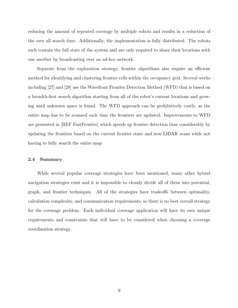


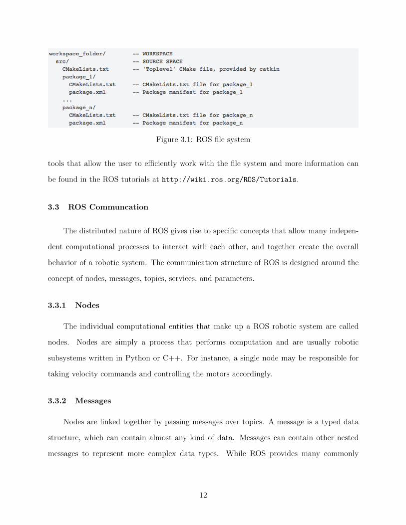


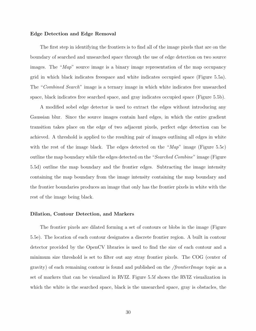


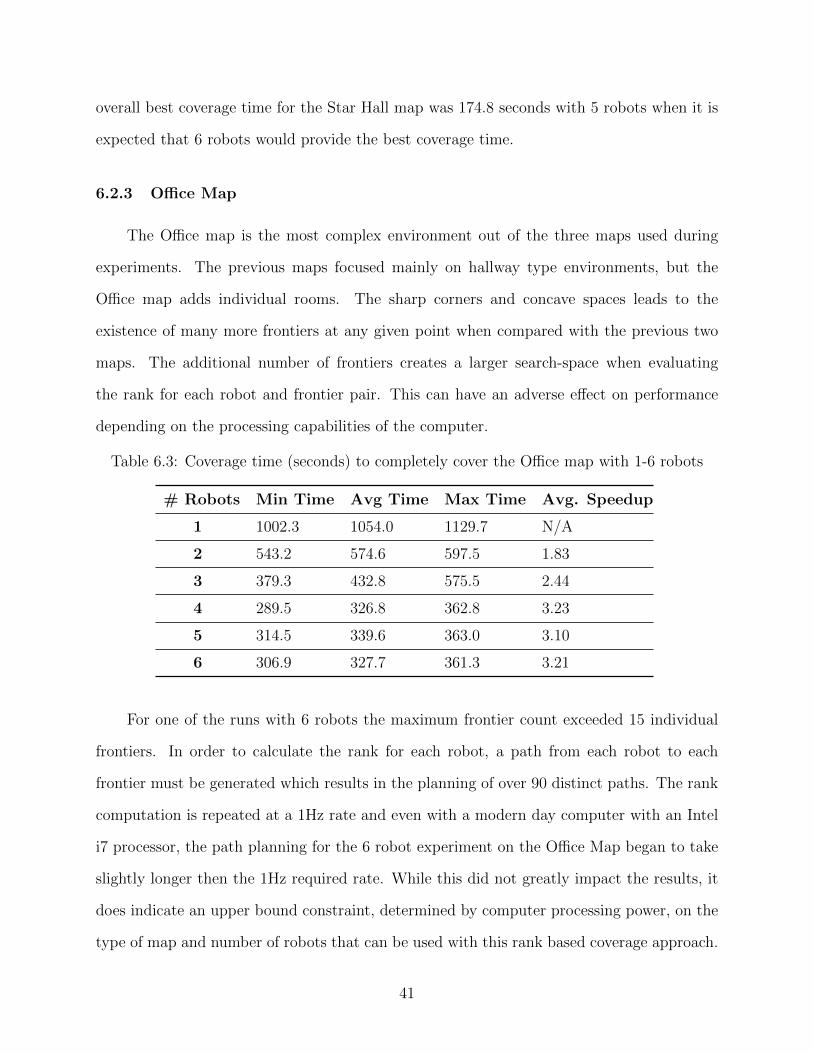


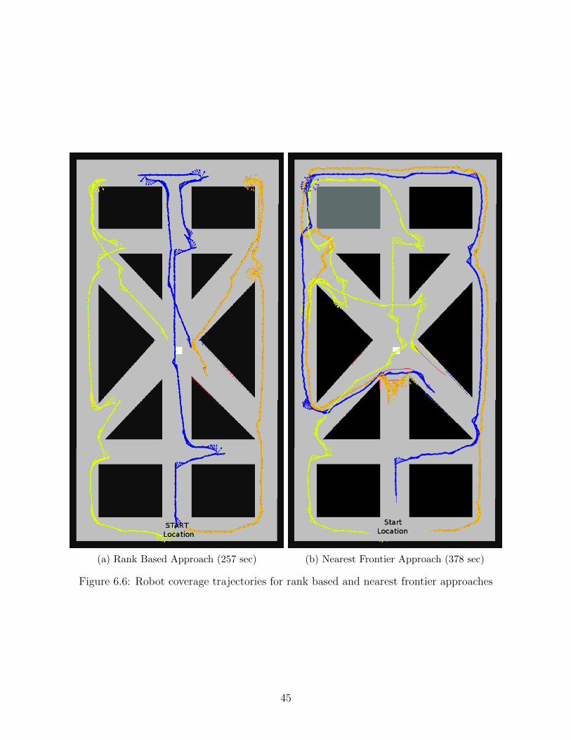


![Towards A ROS-Based Autonomous Cloud Robotics Platform for ...stefanorosa.it/preprints/etfa2014.pdf · tem (ROS). ROS [4] is an open-source, meta-operating system for robot software](https://static.documents.pub/doc/80x56/5f0b40827e708231d42f987b/towards-a-ros-based-autonomous-cloud-robotics-platform-for-tem-ros-ros-4.jpg)


