1 Multi-Sensor Calibration through Iterative Registration and Fusion Yunbao Huang a, b Xiaoping Qian a† Shiliang Chen a a Mechanical, Materials & Aerospace Engineering Department, Illinois Institute of Technology b CAD Center of Huazhong University of Science & Technology, Wuhan, China Abstract In this paper, a new multi-sensor calibration approach, called iterative registration and fusion (IRF), is presented. The key idea of this approach is to use surfaces reconstructed from multiple point clouds to enhance the registration accuracy and robustness. It calibrates the relative position and orientation of the spatial coordinate systems among multiple sensors by iteratively registering the discrete 3D sensor data against an evolving reconstructed B-spline surface, which results from the Kalman filter- based multi-sensor data fusion. Upon each registration, the sensor data gets closer to the surface. Upon fusing the newly registered sensor data with the surface, the updated surface represents the sensor data more accurately. We prove that such an iterative registration and fusion process is guaranteed to converge. We further demonstrate in experiments that the IRF can result in more accurate and more stable calibration than many classical point cloud registration methods. Keywords: B-spline surface reconstruction, registration, Kalman filter, sensor calibration, iterative closest point (ICP) 1 Introduction Multiple sensors of various modalities and with different sensing resolutions, measurement ranges and uncertainties are increasingly being integrated into one platform to improve the overall sensing speed and coverage, and to reduce the uncertainty. Such multi-sensor systems have found wide applications in terrain surveillance, military reconnaissance, dimensional metrology and shape digitization in reverse engineering [1,13, 23, 28]. In order to effectively integrate and fuse spatial data from different 3D sensors, it is important to know the relative position and orientation of the spatial coordinate systems among these sensors [2, 10]. The calibration of such spatial relationships among different sensors can be decomposed into two tasks: intrinsic calibration where internal sensor parameters are determined and extrinsic calibration where the position and the orientation of a sensor relative to a given coordinate system are determined. In this paper, we assume the intrinsic calibration has been properly conducted and we focus on the extrinsic calibration. Among many methods for extrinsic calibration [3, 6, 11, 32, 48], sensor data registration through the iterative closest point (ICP) method or its variants is a common † Xiaoping Qian is the corresponding author and his email is [email protected].
Transcript
1
Multi-Sensor Calibration through Iterative Registration and Fusion
Yunbao Huanga, b Xiaoping Qiana† Shiliang Chen a
a Mechanical, Materials & Aerospace Engineering Department, Illinois Institute of Technology
bCAD Center of Huazhong University of Science & Technology, Wuhan, China
Abstract In this paper, a new multi-sensor calibration approach, called iterative registration and fusion (IRF), is presented. The key idea of this approach is to use surfaces reconstructed from multiple point clouds to enhance the registration accuracy and robustness. It calibrates the relative position and orientation of the spatial coordinate systems among multiple sensors by iteratively registering the discrete 3D sensor data against an evolving reconstructed B-spline surface, which results from the Kalman filter-based multi-sensor data fusion. Upon each registration, the sensor data gets closer to the surface. Upon fusing the newly registered sensor data with the surface, the updated surface represents the sensor data more accurately. We prove that such an iterative registration and fusion process is guaranteed to converge. We further demonstrate in experiments that the IRF can result in more accurate and more stable calibration than many classical point cloud registration methods.
1 Introduction Multiple sensors of various modalities and with different sensing resolutions, measurement ranges and uncertainties are increasingly being integrated into one platform to improve the overall sensing speed and coverage, and to reduce the uncertainty. Such multi-sensor systems have found wide applications in terrain surveillance, military reconnaissance, dimensional metrology and shape digitization in reverse engineering [1,13, 23, 28].
In order to effectively integrate and fuse spatial data from different 3D sensors, it is important to know the relative position and orientation of the spatial coordinate systems among these sensors [2, 10]. The calibration of such spatial relationships among different sensors can be decomposed into two tasks: intrinsic calibration where internal sensor parameters are determined and extrinsic calibration where the position and the orientation of a sensor relative to a given coordinate system are determined. In this paper, we assume the intrinsic calibration has been properly conducted and we focus on the extrinsic calibration. Among many methods for extrinsic calibration [3, 6, 11, 32, 48], sensor data registration through the iterative closest point (ICP) method or its variants is a common
† Xiaoping Qian is the corresponding author and his email is [email protected].
Xiaoping Qian
Text Box
Accepted for publication in Journal Computer-Aided Design, October 6, 2008
2
choice [3, 4, 32] since it requires neither precise knowledge of the geometry of the calibration artifacts nor explicit data correspondence from different sensor data.
However, the calibration result from such a point based registration method is affected by the amount of sensor data and the level of data noise. This problem becomes especially severe in a multi-sensor platform where data density and variance from different sensors vary significantly.
In order to ensure accurate and robust calibration of multiple sensors, in this paper, we present a new approach for multi-sensor calibration. The basis of our approach is two-fold: a) a continuous surface reconstructed from the sensor data provides a more accurate geometry for data registration than the discrete point cloud; b) the surface reconstructed from multiple sensor data is more accurate than that from any single sensor data. We call our approach iterative registration and fusion (IRF). The core idea of the IRF is to iterate the following two steps:
1. Using the ICP algorithm [3] to register different sensor data against a reconstructed surface to achieve accurate and robust alignment for the ensuing point-surface fusion.
2. Using the Kalman filter to fuse the newly aligned sensor data with the previously reconstructed surface to obtain an updated, accurate surface for the subsequent point-surface registration.
The main contribution of this paper is the following.
• We develop a new approach, IRF, for aligning point cloud data of different sensor characteristics such as sampling density and uncertainty (variance). Compared with the original ICP algorithm [3] and its variants such as point-plane registration [6], our novelty lies in the use of an extra fusion process (the second step above) that generates a smooth surface from the aligned multi-sensor data for subsequent point-surface registration. Unlike typical point-surface registration [3, 29] where a surface, often nominal, is given (e.g. measurement data points are to be aligned with the nominal shape model to determine the part shape deviation in metrology applications), the surface in IRF is reconstructed from the points and dynamically evolves as the registration process proceeds. We demonstrate that a) point-surface registration based on the surface reconstructed from point clouds leads to more accurate registration than these ICP variants; b) the IRF results in an even more accurate and robust registration.
• We extend the Kalman filter-based B-spline surface reconstruction [18, 19, 42] into the IRF process. More specifically, we develop a formulation that enables B-spline surface based data fusion, data withdrawal and data registration.
• We further prove and demonstrate that the IRF process is guaranteed to converge to a minimum error. This convergence property facilitates the selection of the initial surface model by checking the accuracy of the surface after the process is converged.
The remainder of this paper is organized as follows. Section 2 reviews prior work in sensor calibration and 3D data registration. Section 3 presents the mathematical formulations for surface-based data fusion, data withdrawal, and data registration. Section 4 describes the overall iterative registration and fusion method. Section 5 gives the
3
experimental results. Section 6 discusses the convergence theorem and how IRF performs under different conditions. This paper concludes in Section 7.
2 Literature review During the object digitization process, complex 3D objects often require sensing from multiple views or several sensors [2, 35]. Multi-sensor calibration typically includes two steps, intrinsic calibration to determine each individual sensor’s internal parameters [36, 37] and data bias [15,16] and extrinsic calibration to determine the relative position and orientation between sensors [28]. In this paper, we concentrate on the extrinsic calibration among sensors.
Multiple methods are available for registering multi-view or multi-sensor data into one common coordinate system. Pair-wise data registration using point-to-point ICP has been widely used [3, 4, 6, 11, 24, 25, 32, 33, 45, 48] and performs well under an appropriate initial orientation and with sufficient data density and low data noise. The algorithmic convergence of these variants is analyzed in [29]. Even though point-surface registration has been discussed in many of these approaches, they assume the surface is given.
Besides the pair-wise correspondence method based on closest points between two data sets, shape features such as spin images (oriented point-normal distribution) [20], linear features [39], integral volume descriptors [12], and invariant features (curvature, moment invariants, spherical harmonics invariants) [34] have also been extracted and used to build the optimal correspondence between a set of point clouds, and followed by the point-to-point ICP to obtain optimal registration.
Since the pair-wise registration for multi-view or multi-sensor data may result in the accumulation of registration error [2, 10], methods have been proposed to improve the overall registration accuracy through a registration network of multi-view data error distribution [2,10], pair-wise alignment constraints [30], optimally distributing the error along the registration cycles [35], force-based optimization [9], and manifold optimization [22].
To get higher registration accuracy, a method combining surface reconstruction and registration is recently proposed in [50]. However, different noise levels are not considered in the surface reconstruction. In our approach, surface reconstruction is formulated as a multi-sensor data fusion process, and different noise levels are considered to obtain a more accurate fusion surface. In addition, our iterative process of multi-sensor data fusion and registration is guaranteed to converge to a minimum error.
3 Mathematical formulation for surface-based data fusion, and data withdrawal and data registration
The mathematical formulations for surface-based data fusion, data withdrawal and data registration are the key to our IRF method and are described in this section. They include: 1) B-spline surface representation, 2) Kalman filter based data fusion, 3) data withdrawal, and 4) data registration. Although Kalman filter-based surface fusion has been introduced in [18, 21, 42, 43], Kalman filter-based data withdrawal is novel and is used in our IRF process.
4
3.1 B-spline surface representation
In the IRF method, the underlying surface for data fusion and registration can be of planar, cylindrical or free-form B-spline surfaces. Without loss of generality, we use the B-spline as the basic surface representation for our introduction of the IRF method since the B-spline surface can represent free-form surfaces and has been widely used in product design and manufacturing. A brief discussion on other types of surfaces is also provided in Section 3.5.
A bi-cubic B-spline surface has the form:
∑∑= =
=u vn
i
n
jijji vBuBvuS
1 1
)()(),( P , (1)
where B is the B-spline shape function and ijP is the ij -th control point (number of control points is vu nnn ×= ). The equation can also be expressed in a matrix form:
PA ⋅=),( vuS , (2) where A is the B-spline shape function vector (of dimension n ), and P represents the collection of control points (of dimension n ). See [27] for details on the B-spline surface representation.
3.2 Data fusion
In order to fuse multi-sensor data which has different sensor noise (we assume that the noise is independent, white and Gaussian) into a B-spline surface, we choose the Kalman filter (a recursive least-squares method) [44] to produce the optimal estimate of the surface in a least-squares sense. Given a sensor measurement z on the surface ),( vuS with parameters ),( zz vu , Eq.2 tells us its position is
ε+⋅= PA zz , (3) where zA is the B-spline shape function matrix, and ε is the measurement noise. In the terminology of the Kalman filter, the above B-spline surface equation represents a linear system between the internal surface state and external observations z [42, 43]. That is, the collection of control points P constitutes the internal state of the object shape, the measurement z with its covariance forms the external observations of the B-spline surface, and zA corresponds to the measurement matrix. Then the Kalman gain [18 ]:
( ) 1
11
−Λ+=−− z
Tzz
Tzl ll
AΛAAΛK PP , (4)
where lK is the l -th step Kalman gain, 1−lPΛ is the covariance of state 1−lP at the ( 1−l )-th
step, and zΛ is the variance of measurement z. The surface state and covariance updating equation are:
ll zzl vu PP ΛAKIΛ or (b) ( ) ( ) ( )( ) ( )zzzzzT vuvu
ll,, 111
1AAΛΛ PP
−−− Λ+=−
. (6)
Eqs. 5 and 6 allow incremental surface update with one measurement z from a surface 1−lS which is defined by control points 1−lP through Eq.2. We denote such an incremental
fusion for surface updating as
5
ll SzS →⊕−1 , (7) where lS is the updated surface defined by the state lP . Given a point cloud },,{ 1 mzzQ L= and the initial surface estimate 0S , we can obtain the final updated surface mS with Eq.7 by
mm SzzzS →⊕⊕⊕ )))((( 210 L . (8) The Eq.8 can be denoted as mSQS →⊕0 . (9) From Eqs. 5 and 6, we can obtain the fusion result efficiently in a batch processing mode [18] from Q and 0S by
( ) ( ) ( ) ( ) ,1
10
11
1
1100 ⎟⎟
⎠
⎞⎜⎜⎝
⎛ Λ+⎟⎟⎠
⎞⎜⎜⎝
⎛ Λ+= ∑∑=
−−−
=
−−m
iiz
Tz
m
izz
Tzm z
iiiiiAPΛAAΛP PP (10)
( ) ( )1
1
110
−
=
−−⎟⎟⎠
⎞⎜⎜⎝
⎛ Λ+= ∑m
izz
Tz iiim
AAΛΛ PP . (11)
where m is the number of measurements, 0S is the initial surface which is defined by 0P and its covariance
0PΛ . The resulting surface mS is represented by mP and its covariance
mPΛ , iz is the th−i measurement, izA is the B-spline shape function matrix
relating to the measurement iz , and izΛ is the variance of iz . Note that the fusion process
is order independent: each term in the summation depends only the (u,v) parameters and measurement iz .
3.3 Data withdrawal
During the IRF process, the sensor points fused into the surface model need to be replaced with the updated coordinates after each new registration. Such replacement will involve a data withdrawal process that withdraws the old data coordinates from the surface model and a data fusion process that adds the new data coordinates into the surface model. Data fusion can be conducted as described above. The data withdrawal process for removing the fused data from the fused surface is described below. Assuming the fused surface kS at step k is defined with the state kP and its covariance
kPΛ , we can withdraw a measured point z with parameter ),( zz vu from the fused surface through the following equations (Lemma 1 in the Appendix contains the detailed proof).
( )kzkkk z PAKPP −′+=+1 and ( )kk zk PP ΛAKIΛ ′−=
+1 , (12)
where ( ) 1−+Λ−⋅=′ Tzzz
Tzk kk
AΛAAΛK PP .
Here we denote the data withdrawal operation for the updated surface 1+kS from the fused surface kS as
kS Θ 1+= kSz . (13) Given a point cloud { }mzzzQ L21,= and its fused surface mS , we can withdraw Q from mS and obtain the surface mmS + after withdrawal through Eq.13 by
(( mS Θ L)1z )Θ mmm Sz +→ . (14)
6
Eq.14 can be denoted as mS Θ mmSQ +→ . (15) Eq. 12 and Eqs. 5 and 6 are structurally similar (and only differ in zz Λ−→Λ ). Similar to the batch mode of data fusion (Eqs. 10 and 11), we can obtain the withdrawn surface mmS + in an efficient batch method for the withdrawal of point cloud Q from the fused surface
mS by
( ) ( ) ( ) ( ) ,1
111
1
11⎟⎟⎠
⎞⎜⎜⎝
⎛ Λ−⎟⎟⎠
⎞⎜⎜⎝
⎛ Λ−= ∑∑=
−−−
=
−−+
m
iiz
Tzm
m
izz
Tzmm z
iimiiimAPΛAAΛP PP (16)
( ) ( )1
1
11−
=
−−⎟⎟⎠
⎞⎜⎜⎝
⎛ Λ−= ∑+
m
izz
Tz iiimmm
AAΛΛ PP . (17)
where mm+\P and its covariance mm+PΛ represents the surface mmS + after withdrawal, mP and
its covariance mPΛ represents the fused surface mS , iz is the th−i measurement Qzi ∈ ,
izA is the B-spline shape function matrix at the measurement iz , and izΛ is the variance
of iz . As with fusion, withdrawal is order-independent.
3.4 Data registration
Given two sensor data clouds 0Q and iQ for data registration, we minimize the overall distance between the two point clouds. Let jq be the th−j point of iQ , ( )jqTr be the transformed point of jq , and jq~ be the point in 0Q with the closest distance to ( )jqTr . The overall squared error between the two point clouds is
( ) ∑∑==
−⋅−==ii m
jjj
m
jjjdE
1
2
1
2 ~21),~(
21),( tqRqqTqtR r , (18)
where R is a rotation matrix, t is a translation vector, ( )( )jjd qTq r,~ is the distance between the transformed point ( )jqTr and its closest point jq~ in 0Q , and im is the number of data points in iQ . The above process of registering point cloud iQ into 0Q ’s coordinate system can be denoted as
ii QQQ ′→⊗ 0 . (19) where the iQ after the transformation is noted as 'iQ . When data points are sparse or the sensor noise is large, the point-to-point registration may not be accurate. Here we register one point cloud against a fused continuous surface. In Eq.18, the objective function changes to
( ) ( )( ) ( )( )∑∑==
+==1
1
02
1
02 ,21,
21,
m
ij
m
jj SdSdE
i
tqRqTtR r , (20)
where 0S is an initial surface reconstructed from the point-cloud 0Q , jq is the th−j point in iQ , ( )( )jSd qTr,0 is the closest distance between the transformed point ( ) ijj Q∈qqTr , and the surface 0S , which can be evaluated by
( ) ( ) ( )( )vuSdSd jvuj ,,min),( 0
,
0 qTqT rr = . (21)
7
We note the above total squared error as )),(( 0SQE irT and note the registration from point cloud iQ to the surface 0S as
iQ ⊗ ii QS ′→−1 . (22)
3.5 Data fusion, withdrawal and registration on other surfaces
Besides the B-spline representation for free-form surfaces, planes and cylinders are common surfaces in various 3D objects. Typical calibration objects have planar and cylindrical surfaces. The extended Kalman filter for the planar surface is available in [26], and the extended Kalman filter for a cylindrical surface can also be deduced from [49]. Example 4 in Section 5.4 will demonstrate that a mechanical part with planar and cylindrical surfaces can also be used for IRF based multi-sensor calibration.
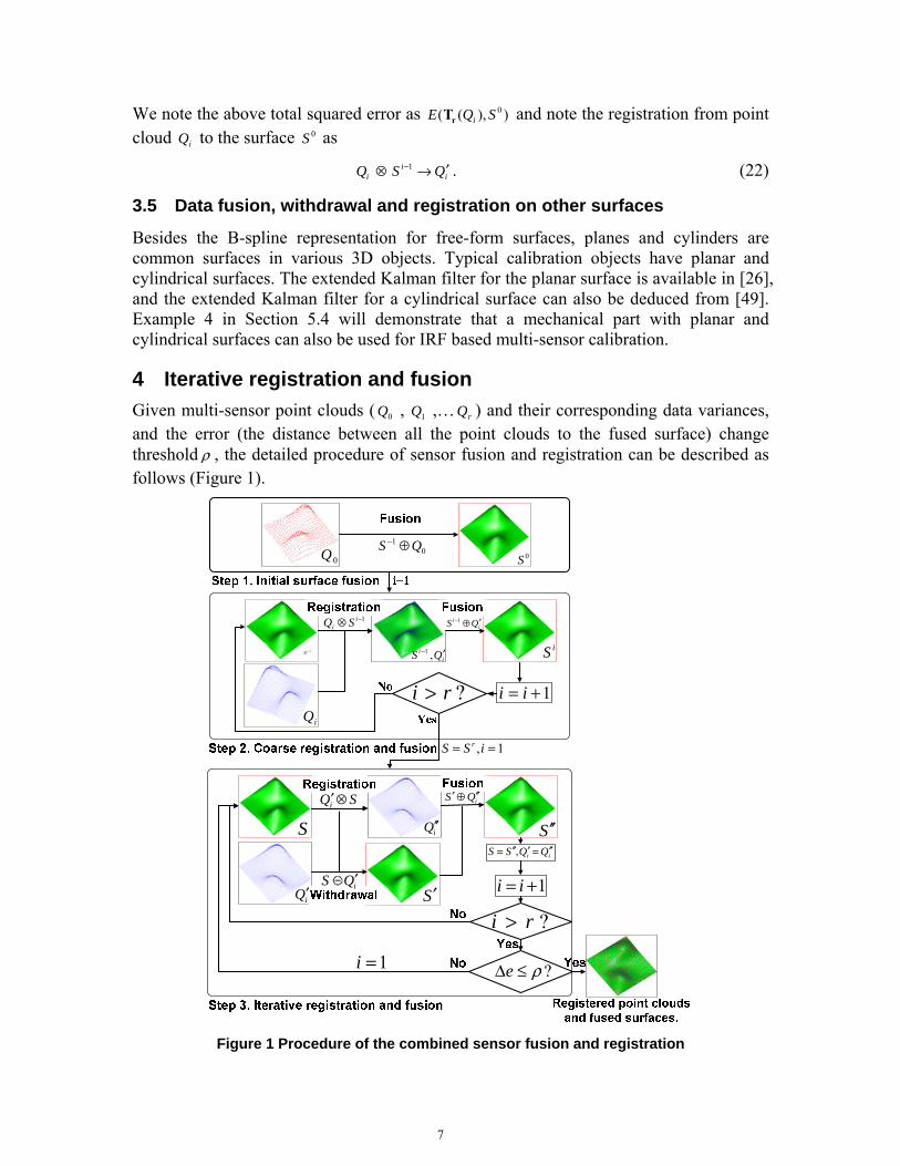
4 Iterative registration and fusion Given multi-sensor point clouds ( 0Q , 1Q ,… rQ ) and their corresponding data variances, and the error (the distance between all the point clouds to the fused surface) change threshold ρ , the detailed procedure of sensor fusion and registration can be described as follows (Figure 1).
0Q 0S
1−iSiS
S iQ ′′
S′
ii QQSS ′′=′′′= ,
S ′′
1, == iSS r
iQ?ri >
1+= ii
1=i
1+= ii
SQi ⊗′
ii QS ′− ,1
1−⊗ ii SQ
01 QS ⊕−
?ri >
iQS ′′⊕′
?ρ≤Δe
ii QS ′⊕−1
iQS ′iQ′
Figure 1 Procedure of the combined sensor fusion and registration
8
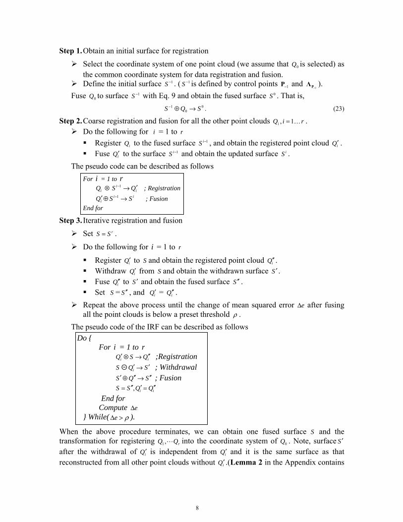
Step 1. Obtain an initial surface for registration
Select the coordinate system of one point cloud (we assume that 0Q is selected) as the common coordinate system for data registration and fusion.
Define the initial surface 1−S . ( 1−S is defined by control points 1−P and 1−PΛ ).
Fuse 0Q to surface 1−S with Eq. 9 and obtain the fused surface 0S . That is, 0
01 SQS →⊕− . (23)
Step 2. Coarse registration and fusion for all the other point clouds riQi K1, = . Do the following for i = 1 to r
Register iQ to the fused surface 1−iS , and obtain the registered point cloud iQ′ . Fuse iQ′ to the surface 1−iS and obtain the updated surface iS .
The pseudo code can be described as follows For i = 1 to r
iQ ⊗ ii QS ′→−1 ; Registration
iii SSQ →⊕′ −1 ; Fusion
End for
Step 3. Iterative registration and fusion
Set rSS = .
Do the following for i = 1 to r
Register iQ′ to S and obtain the registered point cloud iQ ′′ . Withdraw iQ′ from S and obtain the withdrawn surface S ′ . Fuse iQ ′′ to S ′ and obtain the fused surface S ′′ . Set S = S ′′ , and iQ′ = iQ ′′ .
Repeat the above process until the change of mean squared error eΔ after fusing all the point clouds is below a preset threshold ρ .
The pseudo code of the IRF can be described as follows Do {
For i = 1 to r ii QSQ ′′→⊗′ ;Registration
S Θ SQi ′→′ ; Withdrawal SQS ′′→′′⊕′ ; Fusion
, i iS S Q Q′′ ′ ′′= = End for
Compute eΔ } While( ρ>Δe ).
When the above procedure terminates, we can obtain one fused surface S and the transformation for registering rQQ L,1 into the coordinate system of 0Q . Note, surface S ′ after the withdrawal of iQ′ is independent from iQ′ and it is the same surface as that reconstructed from all other point clouds without iQ′ .(Lemma 2 in the Appendix contains
9
detailed proof ). This ensures the final surface after the IRF process is identical as that reconstructed with all the transformed point clouds without the iterative fusion and withdrawal.
In the above procedure, 1) the initial surface 1−S can be interactively defined and then fused with point cloud 0Q . Its covariance can be specified by the user. Alternatively,
1−S can be skipped and 0S can be directly reconstructed from 0Q through Eqs.10 and 11 by setting 0P =0 and its information matrix = 0, 2) the mean squared error is obtained as follows. We assume that all point clouds rQQ ′′ L,1 are in the coordinate system of 0Q . From Eq.9, the fused surface rS from 0Q′ , rQQ ′′ L,1 (here 00 QQ =′ ) and an initial surface estimate 1−S defined by 1−P and
1−PΛ can be obtained by
( )( )( ) rr SQQQS →′⊕′⊕′⊕− L10
1 . (24)
The Kalman filter-based fusion finds the surface estimate rS by minimizing the squared error E between rS and 1−S , and points in 0Q′ , rQQ ′′ L,1 [38]. We have E as
( )( ) ( ) ( ) ( ) ( ) ( ) 21
21 ,,,
0 1
11
1110
11 ∑∑
= =
−−
−−
− −Λ−+−−=′′′−
r
i
m
jrijijz
Trijijr
Tr
rr
i
ijzzSQQQSE PAPAPPΛPP PL
( ).,),(0
1 ∑=
− ′+=r
i
ri
r SQESSE (25)
where rP is the control points defining the surface rS , ijz is the th−j measurement in the th−i point cloud ( )riQi L,0, =′ with variance
ijzΛ and B-spline shape function matrix
ijA , ),( 1 rSSE − is the squared error between 1−S and rS evaluated as ( ) ( ) ( )1
11 1
5.0 −−
− −−×−
PPΛPP P rT
r , and ( )ri SQE ,′ is the squared error between the point cloud iQ′
and rS evaluated as ( ) ( )∑=
− −Λ−i
j
m
jrjjz
Trjj zz
1
1
21 PAPA .
We define the mean squared error )),,,(( 101 r
r SQQQSe ′′′− L as
( ) .,),()),,,((00
1
010
1 ∑∑∑==
−
=
−⎟⎟⎠
⎞⎜⎜⎝
⎛ ′+==′′′r
ii
r
i
ri
rr
ii
rr mSQESSEmESQQQSe L (26)
Since the total number of points ∑=
r
iim
0
of rQQQ ′′′ L10 , is independent of the optimal
estimate rP , minimizing E is equivalent to minimizing )),,,(( 101 r
r SQQQSe ′′′− L .
In Step 3 of the IRF, when all the point clouds are registered and fused, we can obtain the fused surface S and compute the mean squared error ( )( )SQQQSe r ,,,, 10
1 ′′′− L with Eq.26. Then, ( )( )SQQQSe r ,,,, 10
11 ′′′− L can be obtained after the first iteration, ( )( )SQQQSe r ,,,, 10
12 ′′′− L
for the second iteration, and ( )( )SQQQSe rk ,,,, 101 ′′′− L for the k -th iteration. The error change
eΔ between k -th iteration and )1( +k -th iteration can be obtained by
( )( ) ( )( )SQQQSeSQQQSee rkrk ,,,,,,,, 101
1101 ′′′−′′′=Δ −
+− LL . (27)
10
If eΔ < ρ , we terminate the iteration. We show with proof in Section 6.1 that the IRF process monotonically converges.
5 Experimental validation Experiments on two sets of simulated data and two sets of actual sensor data are presented below and are analyzed to show how IRF improves the calibration accuracy and stability. We compare the root-mean-squared (RMS) error of the registration result between three ICP variants, including the original point-to-point ICP [3], the iterative point-to-point ICP for multi-view registration [2, 40], point-to-plane ICP [6], and our approach including a naïve point-surface registration where the surface is simply reconstructed from one point cloud 0Q (without data fusion from other sensor data) and the IRF approach. In our implementation, the distance between a point and a B-spline surface is computed through the subdivision and convex-hull properties of B-splines. We used a commercial geometry modeling kernel, ACIS, to compute it.
5.1 Example 1: simulated surface
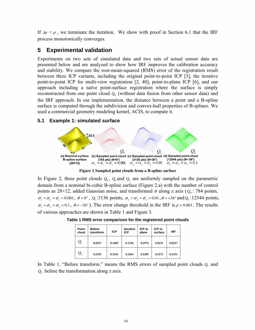
Figure 2 Sampled point clouds from a B-spline surface
In Figure 2, three point clouds 0Q , 1Q and 2Q are uniformly sampled on the parametric domain from a nominal bi-cubic B-spline surface (Figure 2.a) with the number of control points as 28×12, added Gaussian noise, and transformed θ along z axis ( 0Q : 784 points,
0.001x y zσ σ σ= = = , °= 0θ , 1Q :3136 points, 01.0=== zyx σσσ , °+= 36θ and 2Q :12544 points, 1.0=== zyx σσσ , °−= 36θ ). The error change threshold in the IRF is 001.0=ρ . The results
of various approaches are shown in Table 1 and Figure 3. Table 1 RMS error comparison for the registered point clouds
Point- cloud
Before transform. ICP Iterative
ICP ICP to plane
ICP to surface IRF
1Q 0.0227 0.1685 0.1256 0.2976 0.0231 0.0227
2Q 0.2252 0.2541 0.2463 0.2285 0.2272 0.2251
In Table 1, “Before transform.” means the RMS errors of sampled point clouds 1Q and 2Q before the transformation along z axis.
11
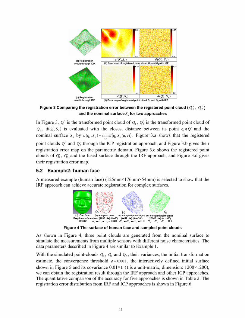
Figure 3 Comparing the registration error between the registered point cloud ( 1Q ′ , 2Q ′ )
and the nominal surface nS for two approaches
In Figure 3, 1Q′ is the transformed point cloud of 1Q , 2Q′ is the transformed point cloud of 2Q , ( )nSQd ,1′ is evaluated with the closest distance between its point 1Qqi ′∈ and the
nominal surface nS by ( )),(.min),(,
vuSqdSqd nivuni = . Figure 3.a shows that the registered
point clouds 1Q′ and 2Q′ through the ICP registration approach, and Figure 3.b gives their registration error map on the parametric domain. Figure 3.c shows the registered point clouds of 1Q′ , 2Q′ and the fused surface through the IRF approach, and Figure 3.d gives their registration error map.
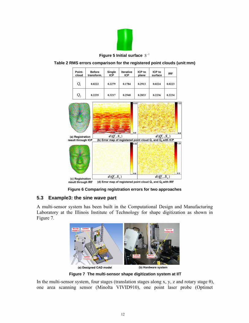
5.2 Example2: human face
A measured example (human face) (125mm×176mm×54mm) is selected to show that the IRF approach can achieve accurate registration for complex surfaces.
Figure 4 The surface of human face and sampled point clouds
As shown in Figure 4, three point clouds are generated from the nominal surface to simulate the measurements from multiple sensors with different noise characteristics. The data parameters described in Figure 4 are similar to Example 1.
With the simulated point-clouds 0Q , 1Q and 2Q , their variances, the initial transformation estimate, the convergence threshold 001.0=ρ , the interactively defined initial surface shown in Figure 5 and its covariance 0.01× I ( I is a unit-matrix, dimension: 1200×1200), we can obtain the registration result through the IRF approach and other ICP approaches. The quantitative comparison of the accuracy for five approaches is shown in Table 2. The registration error distribution from IRF and ICP approaches is shown in Figure 6.
12
Figure 5 Initial surface 1−S
Table 2 RMS errors comparison for the registered point clouds (unit:mm)
Point- cloud
Before transform.
Single ICP
Iterative ICP
ICP to plane
ICP to surface IRF
1Q 0.0222 0.2279 0.1784 0.2913 0.0224 0.0223
2Q 0.2235 0.3217 0.2540 0.2833 0.2236 0.2234
Figure 6 Comparing registration errors for two approaches
5.3 Example3: the sine wave part
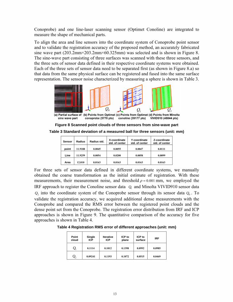
A multi-sensor system has been built in the Computational Design and Manufacturing Laboratory at the Illinois Institute of Technology for shape digitization as shown in Figure 7.
Figure 7 The multi-sensor shape digitization system at IIT
In the multi-sensor system, four stages (translation stages along x, y, z and rotary stage θ), one area scanning sensor (Minolta VIVID910), one point laser probe (Optimet
13
Conoprobe) and one line-laser scanning sensor (Optimet Conoline) are integrated to measure the shape of mechanical parts.
To align the area and line sensors into the coordinate system of Conoprobe point sensor and to validate the registration accuracy of the proposed method, an accurately fabricated sine wave part (203.2mm×203.2mm×60.325mm) was selected and is shown in Figure 8. The sine-wave part consisting of three surfaces was scanned with these three sensors, and the three sets of sensor data defined in their respective coordinate systems were obtained. Each of the three sets of sensor data need to be separated first (as shown in Figure 8.a) so that data from the same physical surface can be registered and fused into the same surface representation. The sensor noise characterized by measuring a sphere is shown in Table 3.
Figure 8 Scanned point clouds of three sensors from sine-wave part
Table 3 Standard deviation of a measured ball for three sensors (unit: mm)
Sensor Radius Radius std. X-coordinate std. of center
Y-coordinate std. of center
Z-coordinate std. of center
point 11.9188 0.0045 0.0055 0.0047 0.0111 Line 11.9259 0.0054 0.0200 0.0058 0.0099 Area 12.010 0.0163 0.0163 0.0163 0.0163
For three sets of sensor data defined in different coordinate systems, we manually obtained the coarse transformation as the initial estimate of registration. With these measurements, their measurement noise, and threshold 001.0=ρ mm, we employed the IRF approach to register the Conoline sensor data 1Q and Minolta VIVID910 sensor data
2Q into the coordinate system of the Conoprobe sensor through its sensor data 0Q . To validate the registration accuracy, we acquired additional dense measurements with the Conoprobe and compared the RMS error between the registered point clouds and the dense point set from the Conoprobe. The registration error distribution from IRF and ICP approaches is shown in Figure 9. The quantitative comparison of the accuracy for five approaches is shown in Table 4.
Table 4 Registration RMS error of different approaches (unit: mm)
Point cloud
Single ICP
Iterative ICP
ICP to plane
ICP to surface IRF
1Q 0.1114 0.1012 0.1398 0.0992 0.0985
2Q 0.09241 0.1193 0.1072 0.0515 0.0469
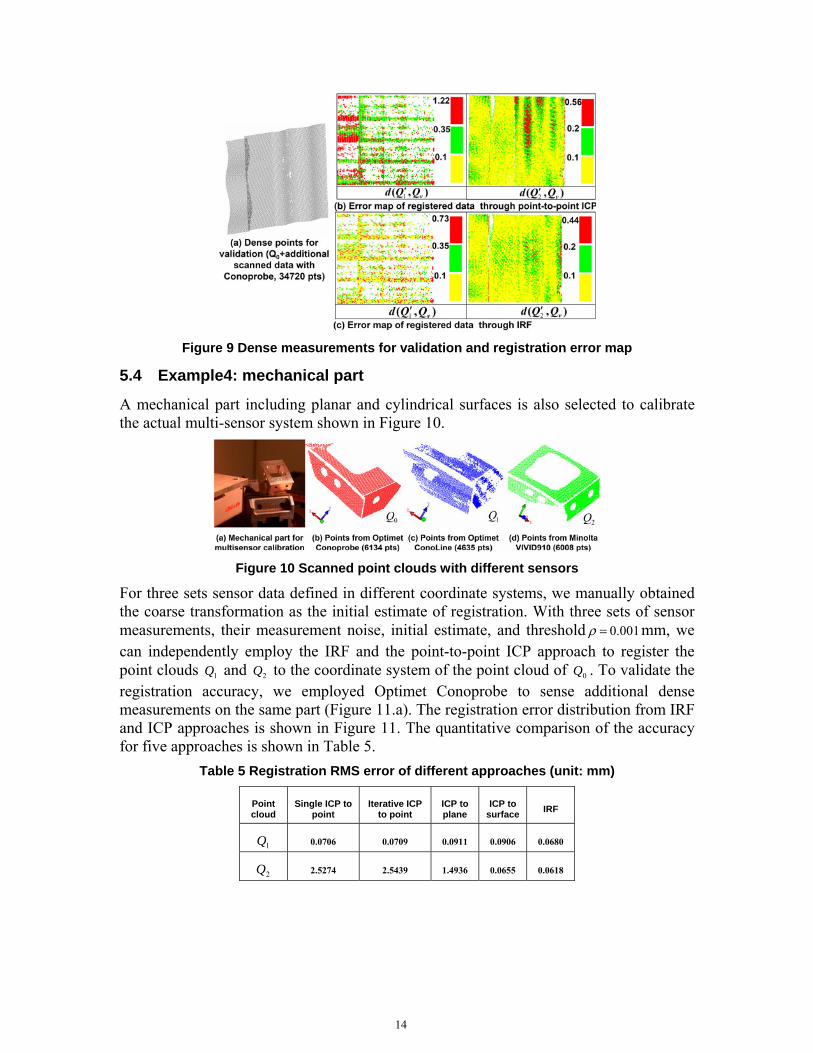
14
Figure 9 Dense measurements for validation and registration error map
5.4 Example4: mechanical part
A mechanical part including planar and cylindrical surfaces is also selected to calibrate the actual multi-sensor system shown in Figure 10.
Figure 10 Scanned point clouds with different sensors
For three sets sensor data defined in different coordinate systems, we manually obtained the coarse transformation as the initial estimate of registration. With three sets of sensor measurements, their measurement noise, initial estimate, and threshold 001.0=ρ mm, we can independently employ the IRF and the point-to-point ICP approach to register the point clouds 1Q and 2Q to the coordinate system of the point cloud of 0Q . To validate the registration accuracy, we employed Optimet Conoprobe to sense additional dense measurements on the same part (Figure 11.a). The registration error distribution from IRF and ICP approaches is shown in Figure 11. The quantitative comparison of the accuracy for five approaches is shown in Table 5.
Table 5 Registration RMS error of different approaches (unit: mm)
Point cloud
Single ICP to point
Iterative ICP to point
ICP to plane
ICP to surface IRF
1Q 0.0706 0.0709 0.0911 0.0906 0.0680
2Q 2.5274 2.5439 1.4936 0.0655 0.0618
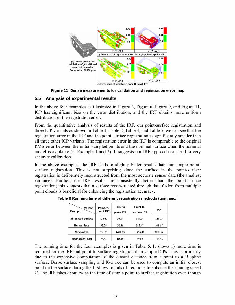
15
Figure 11 Dense measurements for validation and registration error map
5.5 Analysis of experimental results
In the above four examples as illustrated in Figure 3, Figure 6, Figure 9, and Figure 11, ICP has significant bias on the error distribution, and the IRF obtains more uniform distribution of the registration error.
From the quantitative analysis of results of the IRF, our point-surface registration and three ICP variants as shown in Table 1, Table 2, Table 4, and Table 5, we can see that the registration error in the IRF and the point-surface registration is significantly smaller than all three other ICP variants. The registration error in the IRF is comparable to the original RMS error between the initial sampled points and the nominal surface when the nominal model is available (in Example 1 and 2). It suggests our IRF approach can lead to very accurate calibration.
In the above examples, the IRF leads to slightly better results than our simple point-surface registration. This is not surprising since the surface in the point-surface registration is deliberately reconstructed from the most accurate sensor data (the smallest variance). Further, the IRF results are consistently better than the point-surface registration; this suggests that a surface reconstructed through data fusion from multiple point clouds is beneficial for enhancing the registration accuracy.
Table 6 Running time of different registration methods (unit: sec.)
Method Example
Point-to-point ICP
Point-to-
plane ICP
Point-to-
surface ICP IRF
Simulated surface 42.687 33.14 144.74 219.73
Human face 33.75 32.86 513.47 948.67
Sine-wave 331.53 4450.93 1455.42 2890.94
Mechanical part 75.83 82.38 69.03 129.56
The running time for the four examples is given in Table 6. It shows 1) more time is required for the IRF and point-to-surface registration than simple ICPs. This is primarily due to the expensive computation of the closest distance from a point to a B-spline surface. Dense surface sampling and K-d tree can be used to compute an initial closest point on the surface during the first few rounds of iterations to enhance the running speed. 2) The IRF takes about twice the time of simple point-to-surface registration even though
16
the IRF involves multiple times of point-to-surface registration. This is because, after the first point-to-surface registration, the subsequent iteration converges much faster. Since the IRF leads to more accurate but slower registration, it is useful for multi-sensor calibration where the computation is typically done off-line.
6 Discussion In this section, the properties of the proposed IRF approach are discussed, including: 1) its convergence property; 2) its robustness under different number of data points; 3) its robustness under different noise levels (here the noise level refers to the standard deviation of the sensor data); and 4) how it performs with different underlying surface models.
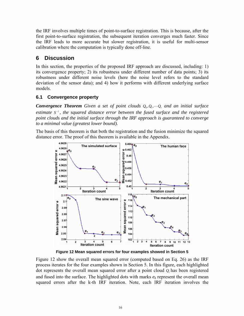
6.1 Convergence property
Convergence Theorem Given a set of point clouds rQQQ L,, 10 and an initial surface estimate 1−S , the squared distance error between the fused surface and the registered point clouds and the initial surface through the IRF approach is guaranteed to converge to a minimal value (greatest lower bound).
The basis of this theorem is that both the registration and the fusion minimize the squared distance error. The proof of this theorem is available in the Appendix.
Figure 12 Mean squared errors for four examples showed in Section 5
Figure 12 show the overall mean squared error (computed based on Eq. 26) as the IRF process iterates for the four examples shown in Section 5. In this figure, each highlighted dot represents the overall mean squared error after a point cloud iQ has been registered and fused into the surface. The highlighted dots with marks ek represent the overall mean squared errors after the k-th IRF iteration. Note, each IRF iteration involves the
17
registration and fusion of r point clouds. From Figure 12, we can see that the overall mean squared errors e in all four examples monotonically converge to minimal values.
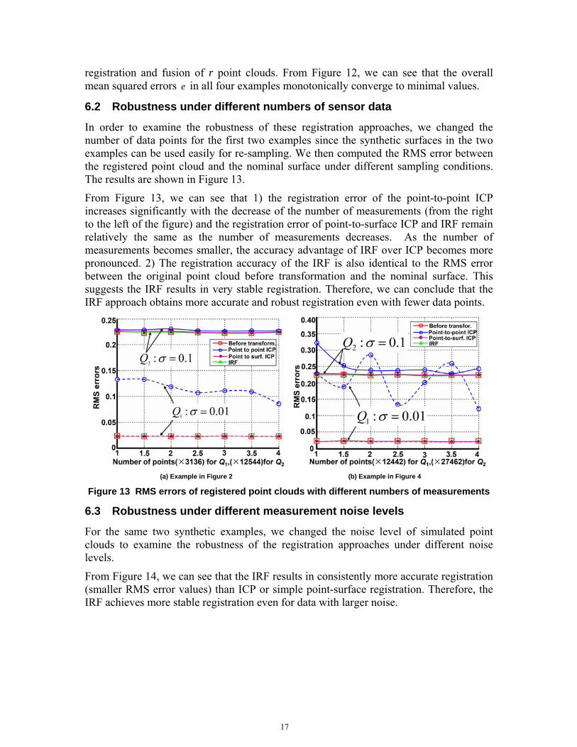
6.2 Robustness under different numbers of sensor data
In order to examine the robustness of these registration approaches, we changed the number of data points for the first two examples since the synthetic surfaces in the two examples can be used easily for re-sampling. We then computed the RMS error between the registered point cloud and the nominal surface under different sampling conditions. The results are shown in Figure 13.
From Figure 13, we can see that 1) the registration error of the point-to-point ICP increases significantly with the decrease of the number of measurements (from the right to the left of the figure) and the registration error of point-to-surface ICP and IRF remain relatively the same as the number of measurements decreases. As the number of measurements becomes smaller, the accuracy advantage of IRF over ICP becomes more pronounced. 2) The registration accuracy of the IRF is also identical to the RMS error between the original point cloud before transformation and the nominal surface. This suggests the IRF results in very stable registration. Therefore, we can conclude that the IRF approach obtains more accurate and robust registration even with fewer data points.
(a) Example in Figure 2 (b) Example in Figure 4
Figure 13 RMS errors of registered point clouds with different numbers of measurements
6.3 Robustness under different measurement noise levels
For the same two synthetic examples, we changed the noise level of simulated point clouds to examine the robustness of the registration approaches under different noise levels.
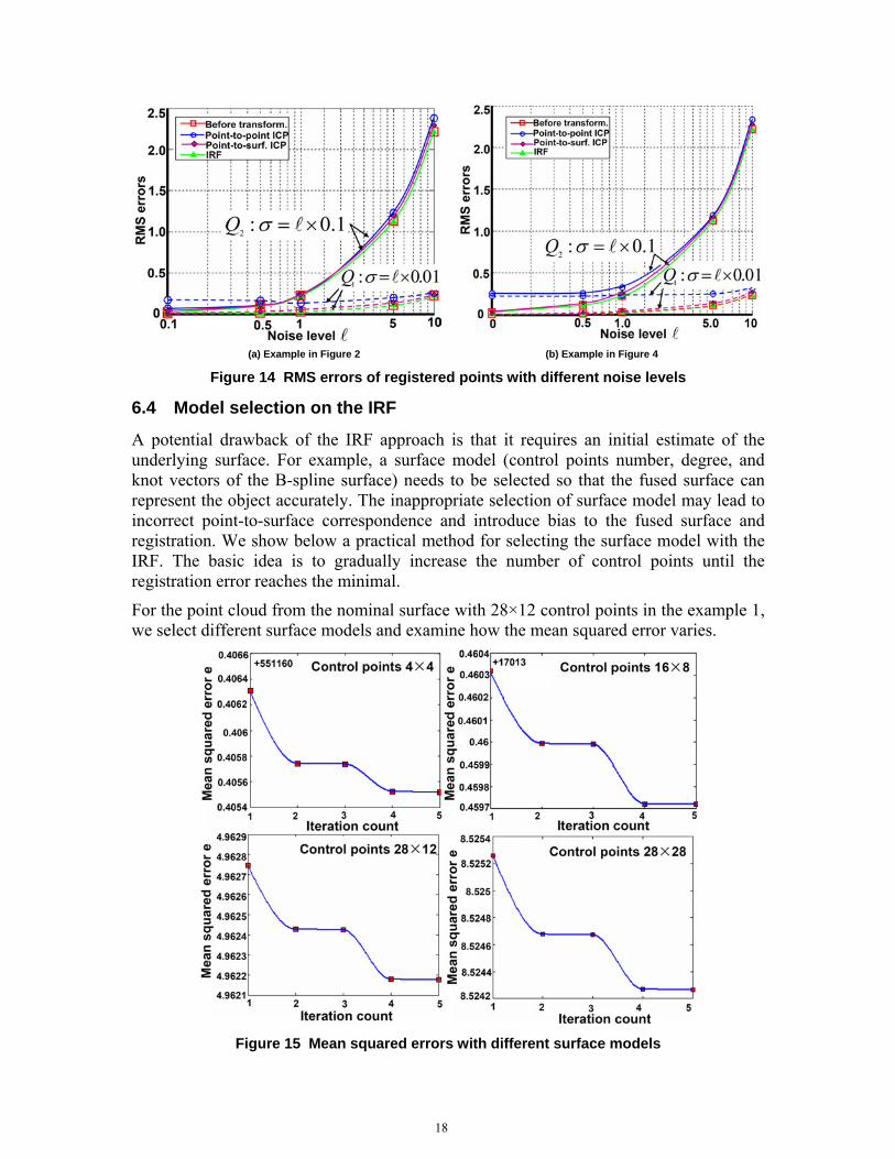
From Figure 14, we can see that the IRF results in consistently more accurate registration (smaller RMS error values) than ICP or simple point-surface registration. Therefore, the IRF achieves more stable registration even for data with larger noise.
18
(a) Example in Figure 2 (b) Example in Figure 4
Figure 14 RMS errors of registered points with different noise levels
6.4 Model selection on the IRF
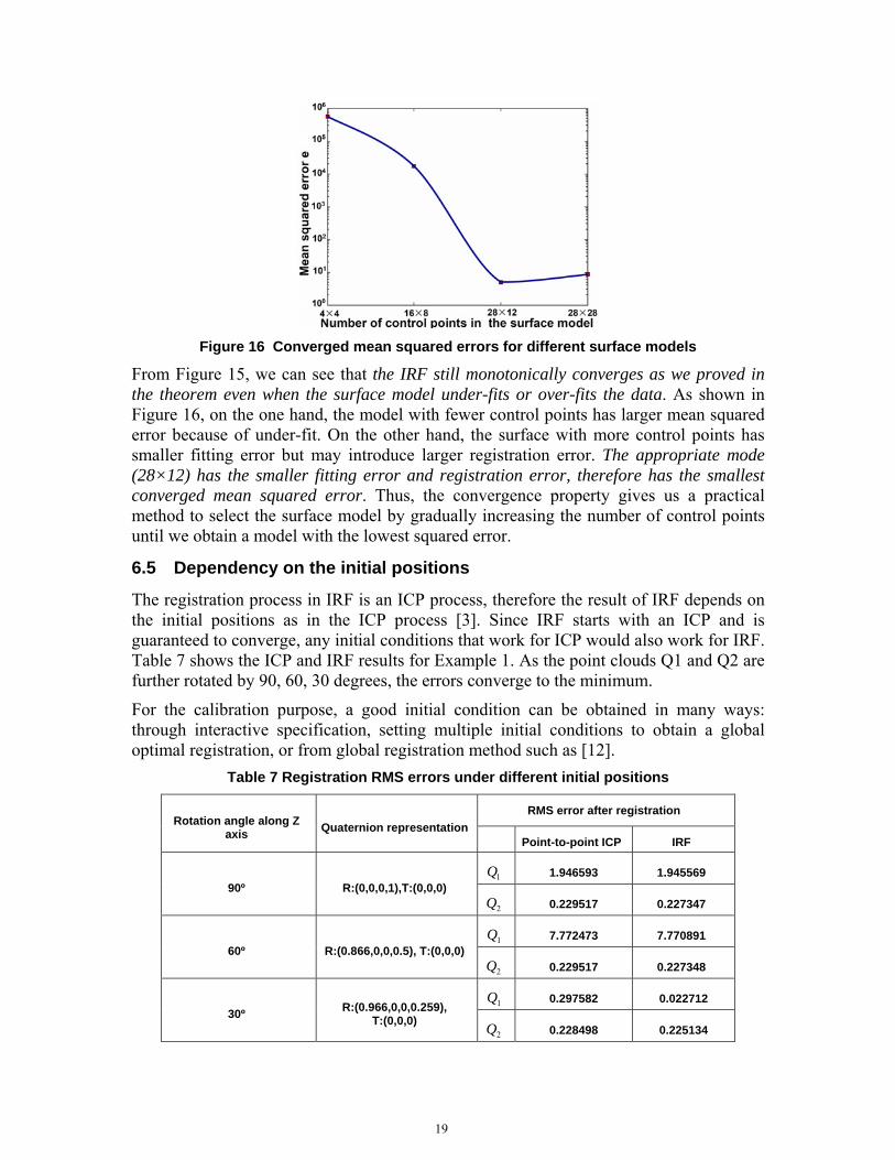
A potential drawback of the IRF approach is that it requires an initial estimate of the underlying surface. For example, a surface model (control points number, degree, and knot vectors of the B-spline surface) needs to be selected so that the fused surface can represent the object accurately. The inappropriate selection of surface model may lead to incorrect point-to-surface correspondence and introduce bias to the fused surface and registration. We show below a practical method for selecting the surface model with the IRF. The basic idea is to gradually increase the number of control points until the registration error reaches the minimal.
For the point cloud from the nominal surface with 28×12 control points in the example 1, we select different surface models and examine how the mean squared error varies.
Figure 15 Mean squared errors with different surface models
19
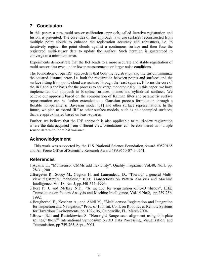
Figure 16 Converged mean squared errors for different surface models
From Figure 15, we can see that the IRF still monotonically converges as we proved in the theorem even when the surface model under-fits or over-fits the data. As shown in Figure 16, on the one hand, the model with fewer control points has larger mean squared error because of under-fit. On the other hand, the surface with more control points has smaller fitting error but may introduce larger registration error. The appropriate mode (28×12) has the smaller fitting error and registration error, therefore has the smallest converged mean squared error. Thus, the convergence property gives us a practical method to select the surface model by gradually increasing the number of control points until we obtain a model with the lowest squared error.
6.5 Dependency on the initial positions
The registration process in IRF is an ICP process, therefore the result of IRF depends on the initial positions as in the ICP process [3]. Since IRF starts with an ICP and is guaranteed to converge, any initial conditions that work for ICP would also work for IRF. Table 7 shows the ICP and IRF results for Example 1. As the point clouds Q1 and Q2 are further rotated by 90, 60, 30 degrees, the errors converge to the minimum.
For the calibration purpose, a good initial condition can be obtained in many ways: through interactive specification, setting multiple initial conditions to obtain a global optimal registration, or from global registration method such as [12].
Table 7 Registration RMS errors under different initial positions
RMS error after registration Rotation angle along Z
7 Conclusion In this paper, a new multi-sensor calibration approach, called iterative registration and fusion, is presented. The core idea of this approach is to use surfaces reconstructed from multiple point clouds to enhance the registration accuracy and robustness, i.e. to iteratively register the point clouds against a continuous surface and then fuse the registered multi-sensor data to update the surface. Such iteration is guaranteed to converge to a minimum error.
Experiments demonstrate that the IRF leads to a more accurate and stable registration of multi-sensor data even under fewer measurements or larger noise conditions.
The foundation of our IRF approach is that both the registration and the fusion minimize the squared distance error, i.e. both the registration between points and surfaces and the surface fitting from point-cloud are realized through the least-squares. It forms the core of the IRF and is the basis for the process to converge monotonically. In this paper, we have implemented our approach in B-spline surfaces, planes and cylindrical surfaces. We believe our approach based on the combination of Kalman filter and parametric surface representation can be further extended to a Gaussian process formulation through a flexible non-parametric Bayesian model [31] and other surface representations. In the future, we plan to extend IRF to other surface models, such as point-sampled surfaces, that are approximated based on least-squares.
Further, we believe that the IRF approach is also applicable to multi-view registration where the data acquired from different view orientations can be considered as multiple sensor data with identical variance.
Acknowledgement This work was supported by the U.S. National Science Foundation Award #0529165
and Air Force Office of Scientific Research Award #FA9550-07-1-0241.
28-31, 2001. 2.Bergevin R., Soucy M., Gagnon H. and Laurendeau, D., “Towards a general Multi-
view registration technique,” IEEE Transactions on Pattern Analysis and Machine Intelligence, Vol.18, No. 5, pp.540-547, 1996.
3.Besl P. J. and McKay N.D., “A method for registration of 3-D shapes”, IEEE Transactions on Pattern Analysis and Machine Intelligence, Vol.14 No.2, pp.239-256, 1992.
4.Boughorbel F., Koschan A., and Abidi M., "Multi-sensor Registration and Integration for Inspection and Navigation," Proc. of 10th Int. Conf. on Robotics & Remote Systems for Hazardous Environments, pp. 102-106, Gainesville, FL, March 2004.
5.Brown B.J. and Rusinkiewicz S. “Non-rigid Range scan alignment using thin-plate splines,” the 2nd International Symposium on 3D Data Processing, Visualization, and Transmission, pp.759-765, Sept., 2004.
21
6.Cheng Y. and Medioni G., “Object modeling by registration of multiple range images,” Proceedings of IEEE International Conference on Robotics and Automation, pp.2724-2729, Sacramento, CA, April, 1991.
7.ConoProbe, http://www.optimet.com/products/conoprobe.html. 8.Dupont R., Keriven R. and Fuchs P., “An improved calibration technique for coupled
single-row telemeter and CCD camera,” Proceedings of Fifth International conference on 3D digital imaging and modeling, pp.89-94, 2005.
9.Eggert D.W., Fitzgibbon A.W. and Fisher R.B., “Simultaneous registration of multiple range views for use in reverse engineering of CAD models,” Computer Vision and Image Understanding, Vol.69, pp.253-272, 1998.
10. Gagnon H., Soucy M., Bergevin R., and Laurendeau D., “Registration of multiple range views for automatic 3-D model building”, Proceedings of 1994 IEEE Computer Society Conference on Computer Vision and Pattern Recognition, pp.581-586, 1994.
11. Gelfand N., Ikemoto L., Rusinkiewicza S. and Levoy M., “Geometrically stable sampling for the ICP algorithm,” The 4th International Conference On 3D-Digital Imaging and Modeling, pp.260-267, Oct., 2003.
12. Gelfand N., Mitra N.J., Guibas L. and Pottmann H., “Robust global registration,” Eurographics symposium on Geometry processing, pp.197-206, 2005.
14. Hall D.L. and Llinas J., “An introduction to multisensor data fusion,” Proceedings of the IEEE, Vol.85, No.1, pp.6-23, 1997.
15. Harding K.G., “Calibration methods for 3D measurement systems,” Proceedings of SPIE on Machine Vision and Three-Dimensional Imaging Systems for Inspection and Metrology, Vol.4189, pp.239-247, 2001.
16. Harding K.G., “Sine wave artifact as a means of calibrating structured light systems,” Proceedings of SPIE, Vol.3835, pp.192-199, 1999.
17. Horn B.K.P. “Closed-form solution of absolute orientation using unit quaternions,” Journal of the Optical Society of America. Vol.4 No.4, pp.629-642, 1987.
18. Huang, Y. and Qian, X., "A dynamic sensing-and-modeling approach to 3D point- and area-sensor integration," ASME Transactions Journal of Manufacturing Science and Engineering, Vol.129, No.3, pp.623-635, 2007.
19. Huang, Y. and Qian, X., “Dynamic B-spline surface reconstruction: Closing the sensing-and-modeling loop in 3D digitization,” Computer Aided-Design Vol.39,No.11, pp.941-952, 2007.
20. Johnson A.E. “Spin-Images: A representation for 3-D surface matching,” Ph.D. thesis, Carnegie Mellon University, 1997.
21. Kohn, R and Ansley, C.F., “A new algorithm for spline smoothing based on smoothing a stochastic process,” SIAM J. Sci. Stat. Comput. Vol.8(1), pp.33-48, 1987.
22. Krishnan S., Lee P., Moore J.B., and Venkatasubramanian S., “Global registration of multiple 3D point sets via optimization-on-a-manifold,” Eurograhics Symposium on Geometry Processing, pp.1-11, 2005.
23. Majlak M. “Quality measurement: managing multisensor technology for CMMS”, Quality Magazine, Vol.44, No.9, pp.34-37, 2005.
24. Masuda T. and Yokoya N., “A robust method for registration and segmentation of multiple range images,” CAD-Based Vision Workshop, Proceedings of the 1994 Second, pp.106-113, 1994.
22
25. Okatani, I.S. and Deguchi K., “A method for fine registration of multiple view range images considering the measurement error properties,” Computer Vision and Image Understanding. Vol.87, pp.66-77, 2002.
26. Pabst Joost van Lawick van, Krekel P.F., “Multi sensor data fusion of points, line segments and surface segments in 3D space,” SPIE Vol.2059, Sensor fusion VI, pp.190-201, 1993.
27. Piegl, L. and Tiller, W., The NURBS Book, Springer-Verlag, NY, 1997. 28. Pless R. and Zhang Q., “Extrinsic calibration of a camera and laser range finder,”
Technical report, Washington Unveristy in St.Louis-School of Engineering & Applied Science, 2003.
29. Pottmann, H., Huang Q., Yang Y. and Hu S. “Geometry and convergence analysis of algorithms,” International Journal of Computer Vision, Vol.67, No.3, pp.277-296, 2006.
30. Pulli K., “Multi-view registration for large datasets,” Second International Conference on 3D Digital Imaging and Modeling, pp.160-168, Oct.,1999.
31. Rasmussen, C.E. and Williams, C.K., “Gaussian Process for Machine Leaning,” The MIT press, 2006.
32. Rusinkiewics S. and Levoy M., “Efficient variants of the ICP algorithm,” in proceedings of 3D digital imaging and modeling, pp.145~152, 2001.
33. Rusinkiewicz S., Hall-Holt O., and Levoy M., “Real-time 3D Model Acquisition,” ACM Transactions on Graphics Vol.21 No.3, 2002.
34. Sharp G.C., Lee S.W. and Wehe D.K., “ICP registration using invariant features,” IEEE Transactions on Pattern Analysis and Machine Intelligence, Vol.24, No.1, pp.90-102, 2002.
35. Sharp G.C., Lee S.W. and Wehe D.K., “Multiview registration of 3D scenes by minimizing error between coordinate frames,” IEEE Transactions on Pattern Analysis and Machine Intelligence, Vol.26 No.8, pp.1037-1050, 2004.
36. Shen T. and Menq C., “Automatic camera calibration for a multiple sensor integrated coordinate measurement system,” IEEE Transactions on Robotics and Automation Vol.17, No.4, pp. 502-507, 2001.
37. Smith K.B. and Zheng Y., “Point laser triangulation probe calibration for coordinate metrology,” ASME Transactions Journal of Manufacturing Science and Engineering. Vol.122, 2000.
38. Sorenson H.W., “Least-squares estimation: from Gauss to Kalman,” IEEE Spectrum, Vol.7, pp.63-68, 1970.
39. Stamos I. and Leordeanu M. “Automated feature based range image registration of urban scenes of large scale”, IEEE International conference of computer vision and pattern recognition, pp.555-561, 2003.
40. Stoddart A.J. and Hilton A., “Registration of multiple point sets,” International Conference of Pattern and Recognition, pp.40-44, 1996.
41. Tylavsky D.J. and Sohie G.R.L. “Generalization of the matrix inversion lemma,” Proceedings of the IEEE, Vol.74, Iss.7, pp.1050-1052, 1986.
42. Wang, Y.F. and Wang, J.F., “On 3D Model Construction by Fusing Heterogeneous Sensor Data,” CVGIP 60(2), pp.210-229, 1994.
43. Wang,Y.F., “A New Method for Sensor Data Fusion in Machine Vision,” SPIE Vol. 1570 Geometric Methods in Computer Vision, 1991, pp. 31 -42, 1991.
23
44. Welch G. and Bishop G., “An introduction to the Kalman Filter,” Technical report, TR-95-041, Department of Computer Science, University of North Carolina at Chapel Hill, 2004.
45. Wen G., Zhu D., Xia S., and Wang Z., “Total least squares fitting of point sets in m-d,” Computer Graphics International 2005, pp.22-24,June 2005.
46. Xie Z., Wang J. and Zhang Q., “Complete 3D measurement in reverse engineering using multi-probe system,” International Journal of Machine Tools & Manufacture, pp. 1474-1485, 2005.
47. Yan, Z., Yang, B., and Menq, C., "Uncertainty analysis and variation reduction of three dimensional coordinate metrology, Part 1: geometric error decomposition," International Journal of Machine Tools & Manufacture, Vol. 39, pp. 1199- 1217, 1999.
48. Zhang Z. “Iterative point matching for registration of free-form curves and surfaces,” International Journal of Computer Vision, Vol.13 No.2, pp.119-152, 1994.
49. Zhang Z. “Parameter Estimation Techniques: A Tutorial with Application to Conic Fitting,” Image and Vision Computing, Vol.15, No.1, pp.59-76, 1997.
50. Huang Q., Adams B. and Wang M., “Bayesian surface reconstruction via iterative scan alignment to an optimized prototype,” In: Proc. 5th Eurographics Symposium on Geometry Processing, Barcelona, pp.213-223, Spain, 2007.
Appendix LEMMA 1 (Data Withdrawal). Assuming a fused surface lS at step l is defined with state lP and its covariance
lPΛ and it is updated from 1−lP and 1−lPΛ with the new
measured point z and variance zΛ . Then we can withdraw z from the fused surface lS by
( )ll zl PP ΛΑKIΛ ′−=
−1 and ( )lzlll z PAKPP −′+=−1 ,
where ( ) 1−+Λ−⋅=′ Tzzz
Tzl ll
AΛAAΛK PP .
Proof: From Eq.6 (b), we can obtain
( ) ( ) ( ) zzTzll
AAΛΛ PP111
1
−−− Λ−=−
. (29)
Computing the inverse of both sides of Eq.29, we can obtain the withdrawn surface covariance
1−lPΛ by
( ) ( )( ) 1111
−−− Λ−=− zz
Tzll
AAΛΛ PP .
Reference [41] gives a generalized form of the analogous matrix inversion lemma as
( ) 1111111 )( −−−−−−− −+=− VCUVCBUCCUBVC .
When ( ) 1−=lPΛC , T
zAU = , ( ) 1−Λ= zB , zAV = , we can obtain lPΛC =−1 and
1−lPΛ as
( ) ( )( )( )
lll
lllllllll
zTzzz
Tz
zTzzz
Tzz
Tzzz
Tz
PPP
PPPPPPPPP
ΛAAΛAAΛI
ΛAAΛAAΛΛΛAAΛAAΛΛΛ1
11
1
−
−−
+Λ−−=
+Λ−−=−Λ+=− .
Let ( ) 1−Λ−=′ zTzz
Tzl ll
AΛAAΛK PP , the above equation can be written as
24
( )ll zl PP ΛAKIΛ ′−=
−1. (30)
From Eq.5, we obtain the state lP at the th−l step from the previous state 1−lP and measurement z by
( ) zllzll KPAKIP +−= −1 . (31)
By multiplying ( ) 11
−−lPΛ to Eq.6.a, we obtain
( ) ( )zlllAKIΛΛ PP −=−
−
11
.
Substituting ( )zl AKI − in Eq.31 with ( ) 11
−−ll PP ΛΛ , we obtain
( ) ( ) ( ) ( ) ( )( ). 11
111
11
1111
zzz lllllll lllllllllKΛPΛΛKΛΛPΛΛKPΛΛP PPPPPPPPP
−−
−−−
−−
− +=+=+=−−−
(32)
With ( ) 1−lPΛ in Eq.6.b and lK in Eq.4, ( ) ll
KΛP1− in Eq.32 can be calculated by
( ) ( )( ) ( )( )( )
( )( ) 111
11
1111
11
11
111
−−−
−−
−−−−
Λ=+Λ+ΛΛ=
+ΛΛ+=
+ΛΛ+=
−−
−−
−−−
zTz
Tzzz
Tzzzz
Tz
Tzzz
Tzzz
Tz
Tz
Tzzz
Tzzz
Tzl
ll
ll
llll
AAΛAAΛAA
AΛAAΛAAA
AΛAAΛAAΛKΛ
PP
PP
PPPP
(33)
Substituting Eq.33 into Eq.32, we can obtain
( )( ) ( ) zzz zTzlz
Tzlz
Tzll llllll
11
11
111
111
−−
−−
−−−
− Λ+=Λ+=Λ+=−−
AΛPAΛPΛΛAPΛΛP PPPPPP .
Multiplying ( ) 11
−− ll PP ΛΛ to both sides of the above equation, we can obtain
Multiplying both sides of Eq.34 with ( ) 1−lPΛ , we can obtain
( ) ( )zlllAKIΛΛ PP ′−=−
−
11
. (38)
25
Substituting Eq.38 into Eq.37, we can compute 1−lP as
( ) ( )lzllllzll zz PAKPKPAKIP −′+=′+′−=−1 .
LEMMA 2. Let a set of point clouds rQQQ L,, 10 , an initial surface estimate 1−S defined by 1−P and
1−PΛ , and their fusion surface rS defined by rP and rPΛ through Eq.10 and 11.
Then the withdrawn surface =′iS rS Θ iQ is independent of iQ .
Proof: Assume the fused surface from rii QQQQQ ,,,,,, 1110 LL +− and 1−S is S , we can get S by (it can be inferred from Eq.10 and 11)
rii QQQQSS ⊕⊕⊕⊕= +−− LL 110
1 , (39)
and rS by
riiir QQQQQSS ⊕⊕⊕⊕⊕= +−
− LL 1101 . (40)
Eq.40 can be written as
iiriir QSQQQQQSS ⊕=⊕⊕⊕⊕⊕= +−
− LL 1101
Due to 1) =′iS rS Θ iQ , and 2) the proof in Lemma 2, we can get SS i =′ . From Eq.39, we can see S is independent of iQ . Since SS i =′ , we can know that the withdrawn surface =′iS rS Θ iQ is independent of iQ Q.E.D.
LEMMA 3. Let 0S be a surface defined by control points 0P and its covariance0PΛ , and
{ }mzzzQ ,,. 211 L= with variance { }mzzz ΛΛΛ ,,.
21L be one point cloud, the fused surface 1S
defined by control points 1P and variance 1PΛ can be obtained by 1
10 SQS →⊕ , and the
withdrawn surface 0S ′ defined by control points 0P′ and covariance 0PΛ ′ can be obtained
by 1S Θ 01 SQ ′→ , then 0S ′ equals 0S i.e. 0P′ = 0P and
0PΛ ′ = 0PΛ .
Proof: As shown in Eq.10 and 11, the fused surface 1S from 0S and 1Q can be obtained by
( ) ( )
( ) .
,
1
1
11
1
10
11
1
111
01
00
−
=
−−
=
−−−
=
−−
⎟⎠
⎞⎜⎝
⎛ Λ+=
⎟⎠
⎞⎜⎝
⎛ Λ+⎟⎠
⎞⎜⎝
⎛ Λ+=
∑
∑∑m
iiz
Tz
m
iz
Tz
m
izz
Tz
ii
iiiii
AAΛΛ
APΛAAΛP
PP
PP
(41)
From Eq.16 and 17, we can obtain the withdrawn surface 0S ′ from 1S by
( ) ( )
( ) .
,
1
1
11
1
11
11
1
110
10
11
−
=
−−′
=
−−−
=
−−
⎟⎠
⎞⎜⎝
⎛ Λ−=
⎟⎠
⎞⎜⎝
⎛ Λ−⎟⎠
⎞⎜⎝
⎛ Λ−=′
∑
∑∑m
izz
Tz
m
iz
Tz
m
izz
Tz
iii
iiiii
AAΛΛ
APΛAAΛP
PP
PP
. (42)
Substituting Eq.41 into Eq.42, we can obtain
26
( ) ( )
( ) ( ) ( ) ( )
( ) .
,
000
000110
10
1
1
1
1
11
001
1
1
1
10
111
1
11
11
1
1
1
110
PPP
PPPPPP
PP
ΛAAAAΛΛ
PPΛΛAAPΛΛΛΛ
APΛAAAAΛP
=⎟⎠
⎞⎜⎝
⎛ Λ−Λ+=
==⎟⎠
⎞Λ−⎜⎜⎝
⎛⎟⎠
⎞⎜⎝
⎛ Λ+=
⎟⎠
⎞⎜⎝
⎛ Λ−⎟⎠
⎞⎜⎝
⎛ Λ−Λ+=′
−
=
−
=
−−′
−
=
−
=
−−−−
=
−−−
=
−
=
−−
∑∑
∑∑
∑∑∑
m
izz
Tz
m
izz
Tz
m
iz
Tz
m
iz
Tz
m
iz
Tz
m
izz
Tz
m
izz
Tz
iiiiii
iiii
iiiiiiii
Since 00 PP =′ and 00 PP ΛΛ =′ , hence the surface 0S ′ equals 0S .
Theorem (Convergence of IRF) Let an initial surface approximation 1−S and a set of point clouds rQQQ L,, 10 for this surface be given. Then the sequence of means squared errors { }ree ,,0 K between the fused surface and registered point clouds in the IRF, and the initial surface, decreases monotonically.
Proof: In the procedure described in Section 4, the IRF approach includes three main steps, the first and second step are to construct an initial surface for the IRF and to compute coarse registration and fusion of r sets of sensor data. The two steps do not include iteration and always converge. The third step includes an iteration process to obtain the fine registration by iteratively registering the point cloud iQ′ to S and obtain registered point cloud iQ ′′ , withdrawing iQ′ from S , and fusing iQ ′′ to S′ . The following will prove the convergence of this iteration process.
(1) Registration of iQ′ to S .
The registration of iQ′ to S can be noted as ii QSQ ′′→⊗′ , and is obtained by minimizing the squared error ( )( )SQE i ,′rT
( )( ) ( ) i
m
jjjii QzSzdSQQE
i
′′∈=′=′′ ∑=1
2 ,,21,rT ,
where rT is the transformation described in section 3.4, im is number of points in iQ′ , jz is the th−i transformed point, and ( )Szd j , is the minimal distance between the jz and the fused surface S . Let P be the control points of S , and ),( jj vu be the parameter of the closet point of jz on S , ( )Szd j , is calculated by
( ) PA jjj zSzd −=, ,
where jA is the B-spline shape function matrix for jz . Since the registration is to find rT by minimizing ( )( )SQE i ,′rT , Therefore
where ( )SQE i ,′ is the squared error between iQ′ and S , which can be evaluated with Eq. 26.
(2) Withdrawal of iQ′ from S .
27
For the withdrawal of iQ′ from S , we can obtain surface S ′ by S Θ SQi ′→′ . It means that SQS i →′⊕′ (Detailed proof can be seen Lemma 3 ). From Eq.24, the surface S can be
obtained by
SQQQQQS irii →′⊕′⊕′⊕′⊕′⊕ +−− LL 110
1 .
The surface S is obtained through the Kalman filter, it can be also obtained by minimizing the squared error from Eq.26,
( )( ) ),( ),( ),(),( ,,,,,,1
1
0
1110
1 SQESQESQESSESQQQQQSE i
r
ijj
i
jjirii ′+′+′+=′′′′′ ∑∑
+=
−
=
−+−
− LL . (44)
Substituting Eq.43 into Eq.44 , we can obtain
( )( )
( )( )SQQQQQSESQESQESQESSE
SQESQESQESSESQQQQQSE
iriii
r
ijj
i
jj
i
r
ijj
i
jjirii
,,,,,, ),( ),( ),(),(
),( ),( ),( ),(,,,,,,
1101
1
1
0
1
1
1
0
1110
1
′′′′′=′+′+′+≤
′′+′+′+=′′′′′′
+−−
+=
−
=
−
+=
−
=
−+−
−
∑∑
∑∑
LL
LL (45)
Dividing both sides of Eq.45 with ∑=
r
iim
0
, we can obtain
( )( ) ( )( )
( )( ) ( )( )SQQQQQSemSQQQQQSE
SQQQQQSemSQQQQQSE
irii
r
iiirii
irii
r
iiirii
,,,,,,,,,,,,
,,,,,,,,,,,,
1101
0110
1
1101
0110
1
′′′′′=′′′′′≤
′′′′′′=′′′′′′
+−−
=+−
−
+−−
=+−
−
∑
∑
LLLL
LLLL
(45)
(3) The fusion of iQ ′′ to S ′ . For the fusion of iQ ′′ with S ′ , the updated surface S ′′ can be obtained by SQS i ′′→′′⊕′ .
As described in Eq.24, S ′′ can be obtained by
SQQQQQS irii ′′→′′⊕′⊕′⊕′⊕′⊕ +−− LL 110
1 . As shown in Eq.26, the surface S ′′ can be also obtained by minimizing
( )( ) ( ) ( ) ( ) ( )SQESQESQESSESQQQQQSE i
r
ijj
i
jjirii ′′′′+′′′+′′′+′′=′′′′′′′′ ∑∑
+=
−
=
−+−
− ,,,,,,,,,,,,1
1
0
1110
1 LL . (46)
Since S ′′ is the solution with minimal value of Eq.46, we have
− LLLL . (49) Eq.49 means that: from input iQ′ and the surface S , we can obtain the registered point cloud iQ ′′ and the updated surface S ′′ with a smaller mean squared error.
(4) The mean squared error from iQ′ to 1+′iQ . When the iteration is transferred from iQ′ to 1+′iQ , we need to prove the right side of Eq.49 at step 1+i for 1+′iQ equals to the left side of Eq.49 at step i for iQ′ so that the mean squared error monotonically decreases. The following gives the detailed proof. For the registration and fusion with iQ′ , noting SSi = , SS i ′=′ , and SS i ′′=′′ , we can express Eq.49 at step i for iQ′ as
( )( ) ( )( )iiirii
iirii SQQQQQSeSQQQQQSe ,,,,,,,,,,,,,, 110
1110
1 ′′′′′≤′′′′′′′′ +−−
+−− LLLL . (50)
and express Eq.49 at step 1+i for the point cloud 1+′iQ as ( )( ) ( )( )1
11011
1101 ,,,,,,,,,,,,,, +
+−−+
+−− ′′′′′≤′′′′′′′′ i
iiriii
irii SQQQQQSeSQQQQQSe LLLL . (51)
From Eq.48, we can know the left side of Eq.50 can be obtained by
( )( ) ( ) ( ) ( ) ( ) .,,,,,,,,,,,,01
1
0
1110
1 ∑∑∑=+=
−
=
−+−
−⎟⎟⎠
⎞⎜⎜⎝
⎛′′′′+′′′+′′′+′′=′′′′′′′′
r
ii
r
ij
ii
ij
i
j
ij
iiirii mSQESQESQESSESQQQQQSe LL (52)
and the right side of Eq.51 can be computed by
( )( ) ( ) ( ) ( ) ( ) ∑∑∑=+=
++
+
=
++−++−
−⎟⎟⎠
⎞⎜⎜⎝
⎛′+′+′+=′′′′′
r
ii
r
ij
ii
ij
i
j
ij
iiirii mSQESQESQESSESQQQQQSe
02
11
1
0
1111110
1 ,,,,,,,,,, LL . (53)
In the Step 3 of the IRF, we have 1+=′′ ii SS , iQ′ in Eq.53 equals iQ ′′ in Eq.52, then Eq.53 changes to
( )( ) ( )( )( ) ( ) ( ) ( ) ( )
( ) ( ) ( ) ( )( )( ) ,,,,,,,,
,,,,
,,,,,
,,,,,,,,,,,,,,,,,
1101
01
1
0
1
01
2
1
0
1
121011
1101
iirii
r
ii
ii
r
ij
ij
i
j
ij
i
r
ii
ii
r
ij
ij
ij
i
j
ij
i
iiriii
iirii
SQQQQQSe
mSQESQESQESSE
mSQESQESQESQESSE
SQQQQQQSeSQQQQQSe
′′′′′′′′=
⎟⎟⎠
⎞⎜⎜⎝
⎛′′′′+′′′+′′′+′′=
⎟⎟⎠
⎞⎜⎜⎝
⎛′′′+′′′+′′′′+′′′+′′=
′′′′′′′′′=′′′′′
+−−
=+=
−
=
−
=+
+=
−
=
−
++−−+
+−−
∑∑∑
∑∑∑
LL
LLLL
(54)
From Eq.50, 51 and 54, we can see that the mean squared error e is monotonically reduced for any point cloud registration and fusion. Since the mean squared error 0≥e , and e is nonincreasing, then the error change 0→Δε , and the stated IRF approach must monotonically converge to a local minimal solution. Q.E.D.