MULTI-SENSOR FUSION BASED CONTROL FOR AUTONOMOUS OPERATIONS: RENDEZVOUS AND DOCKING OF SPACECRAFT by JONATHAN BRYAN MCDONALD Presented to the Faculty of the Graduate School of The University of Texas at Arlington in Partial Fulfillment of the Requirements for the Degree of MASTER OF SCIENCE IN AEROSPACE ENGINEERING THE UNIVERSITY OF TEXAS AT ARLINGTON December 2006
Transcript
MULTI-SENSOR FUSION BASED CONTROL FOR
AUTONOMOUS OPERATIONS: RENDEZVOUS
AND DOCKING OF SPACECRAFT
by
JONATHAN BRYAN MCDONALD
Presented to the Faculty of the Graduate School of
The University of Texas at Arlington in Partial Fulfillment
8.1 Satellite Initial Conditions for Both Simulations . . . . . . . . . . . . 66
8.2 Sensor Estimation, & Control Parameters for Both Simulations . . . . 67
8.3 Control Law Parameters for Both Simulations . . . . . . . . . . . . . 68
x
Nomenclature
x No marker indicates a true value and/or a scalar
x Bold indicates a vector unless specified otherwise,
all vectors are columns unless otherwise specified
x Hat indicates an estimated value or unit vector (where appropriate)
x Tilde indicates measurement
[NB] Rotation matrix (from B-frame to N-frame)
In×n Appropriately dimensioned identity matrix
[I] 3× 3 Inertia matrix
[a×] Skew symmetric matrix
τ GPS clock bias
β Gyro bias
Superscript
Bx Upper left indicates the reference frame the vector components are expressed in
N, O, T, P - Inertial, Orbit, Target, and Pursuer Frames respectively will be used
xT Upper right T indicates the transpose of the vector/matrix
xM Indicates Fused Master/Global Estimate
PM Indicates Fused Master/Global Covariance
ρ GPS pseudorange measurement
Subscript
GPS, vision Sensor description
i Variable number
s/c Stands for Spacecraft (Spacecraft and Satellite will be used interchangeably)
Master/Global Denotes the Master or Global estimate.
Master and Global will be used interchangeably
xi
CHAPTER 1
INTRODUCTION
For the last half-century, space program engineers and scientists have continu-
ally addressed the problem of spacecraft rendezvous. One early 1960s Gemini Mission
goal was ‘to develop effective methods of rendezvous and docking with other orbiting
vehicles, and to maneuver the docked vehicles in space.’ During Gemini VIII, the
first manned spacecraft successfully rendezvoused and docked on March 16, 1966 [1].
Since that time, spacecraft rendezvous and docking has served multiple pur-
poses, including: return from the moon in the Apollo missions; repair and mainte-
nance of the Hubble Space Telescope by astronauts; and refueling/resupply of space
stations, including the International Space Station (ISS).
Nearly all past satellite servicing missions have been carried out by astronauts
and in a few instances robotic manipulators have aided the mission, but it is both
expensive and dangerous for astronauts to capture uncontrolled spinning satellites
(even slowly spinning satellites). Thus, it is desirable to develop a free-flying robotic
space vehicle capable of carrying out such satellite service missions [2].
One goal of NASA’s Space Launch Initiative (SLI) program is to develop such
a vehicle, a space transportation system with automated rendezvous and docking
generally less expensive and more safe and reliable than today’s Space Shuttle [3].
The Space Shuttle currently uses a partially manual system for rendezvous, but a
fully autonomous rendezvous system could be more dependable and less dangerous
[4].
1
2
Several projects dealing with autonomous rendezvous and docking of orbiting
satellites have been developed over the past decade, including the Progress spacecraft,
Demonstration of Autonomous Rendezvous Technology (DART), and Engineering
Test Satellites VII (ETS-VII).
The Progress spacecraft, a Russian expendable unmanned freighter originally
developed to supply the Russian space stations, is currently being used to help re-
supply the ISS. Though proximity operations1 are monitored and can be overridden
by a backup system on the ISS, each Progress’ rendezvous and docking operation is
capable of being totally autonomous [5]. This procedure, though impressive, is sim-
plified because the ISS (and formally other space stations) is in a controlled orbit, can
control its attitude, and manual control can be implemented by the ISS astronauts if
problems arise.
While the Progress rendezvous can include ISS manual control, DART and ETS-
VII Missions are characterized by two autonomous satellites attempting to rendezvous
and dock. Mitsubishi Electric successfully docked two unmanned satellites (ETS-VII)
for the first time in 1998 under the funding and direction of Japan’s National Space
Development Agency (JAXA). Their test established the feasibility of autonomous
docking of satellites and provided evidential insight for overcoming various mishaps
that could occur [6].
In April 2005, the DART Mission attempted to become the first American
autonomous satellite rendezvous; however, approximately 11 hours into what was to
be a 24-hour mission, DART detected its propellant supply was depleted and it began
a series of maneuvers for departure and retirement. NASA determined most of its
1‘Proximity operations’ are defined as the navigation and control of two or more vehicles thatare operating in the vicinity of each other [4].
3
mission goals were not achieved [7], and autonomous satellite rendezvous continues
to remain a developing technology.
As orbital activity continues to increase, it becomes more and more imperative
that an autonomous space vehicle capable of capturing a tumbling object in orbit be
developed, so that it might remove space debris, service a malfunctioning satellite,
refuel a powerless satellite, and/or install improved technology.
The launch of just one autonomous servicing system maintained in orbit could
provide tremendous savings to the satellite industry by servicing multiple malfunc-
tioning satellites, replacing the current system of launches for every single critical
malfunction. Use of such a system would also eliminate the danger astronauts face
in colliding with satellites as they repair them. However, the development of such a
system is very complex and even tasks such as mission phasing can vary greatly in
complexity.
In a broad perspective, the satellite rendezvous mission must carry out sequen-
tial tasks corresponding to each phase of the mission. Researchers from JAXA have
developed such a phased mission plan using a new system concept called Hyper-
Orbital Servicing Vehicle (HOSV). This system consists of a bulky ‘mother ship’
(which has components similar to a conventional satellite, such as solar panels and
a large communication antenna) and a deployable operation vehicle that is agile and
compact [8].
The HOSV concept has the servicing/rescue vehicle docked at a mother ship
(such as the International Space Station) from which it departs and returns after each
mission. Note: From this point on the rescue satellite will be known as the ‘Pursuer’
and the satellite to be serviced will be known as the ‘Target’. Before a mission is
commenced, knowledge of the Target’s orbit must be obtained; once obtained, the
entire mission can be roughly divided into seven phases, generally outlined as follows:
4
Phase I. Departure from mother ship
Phase II. Orbit transfer to Target’s orbit & long range approach
Phase III. Target identification & motion characterization
Phase IV. Proximity approach including guidance & control for docking
Phase V. Docking & capture
Phase VI. Service & maintenance
Phase VII. Pursuer return to mother ship
The first phase, Phase I, consists of the Pursuer departing from the mother ship. In
Phase II (which can be optimized for fuel or time consumption) the Pursuer transfers
from its docked orbit to that of the Target and approaches the Target’s area until
a positive identification can be made (Phase III). Phase IV begins after the Target
has been positively identified and its motion has been characterized. In this phase,
the Pursuer’s sensors and controllers synchronize the Pursuer’s motion with that of
the Target until the proper docking alignment is achieved. Once accomplished, the
Pursuer can capture and dock with the Target (Phase V). In Phase VI, the Pursuer
services the Target and, finally, the Pursuer separates from the Target and returns to
its mother ship (unless it is a recovery mission, in which case both return) in Phase
VII.
The mission procedure described above is just a general overview of one poten-
tial mission, each segment having several different aspects and levels of complexity.
This thesis research focuses on Phase IV, the Pursuer’s proximity operations just
prior to docking.
To achieve the motion synchronization aspect of Phase IV, the dynamical char-
acteristics (translational and rotational motion) of the Target and Pursuer must be
known. If the Target is in a free-floating orbit, the Pursuer does not have to account
for orbital maneuvers by the Target, but the Target’s rotational motion or spin must
5
be accounted for. All satellites have some type of rotational motion, either for stabi-
lization or caused by gravity gradients or other natural perturbations. However, not
all satellites rotate at the same rate (because of various factors — geometry, mission
design, mechanical failure, disturbances, etc.), affecting the motion synchronization
necessary for rendezvous and capture.
Satellite capture can be roughly categorized into four classifications based upon
the attitude error and rate of the Target. The classifications and categories II, III,
and IV, shown in Figure 1, are called non-cooperative target captures [8]. The
I Satellite with three-axis attitude control- Direct capture by single chaser satellite
equipped with specialized capturing mecha-nism.
II Satellite with gravity gradient stabilization- Direct capture by single chaser satellite
equipped with manipulator.III Slowly tumbling Satellite
- Local motion synchronized capture by agilespace robot.
IV Spinning Satellite- Spinning motion synchronizing capture by agile
space robot.- Capturing after damping target spin rate.
Figure 1.1 Categorization of Satellite Motion.
capture of a spinning satellite (Category IV) is relatively rare, so the remainder of
this thesis will focus on estimation and control to achieve motion synchronization for
docking with a slowly tumbling satellite (Category III).
Attempting to use grasping equipment without accompanying motion synchro-
nization in a satellite capture is not practically feasible unless the Target is tumbling
within the capabilities of the dynamic response of the manipulator, and failure to
grasp the Target could result in detrimental collision. Successful capture, then, can
6
be ensured with a control system combining attitude synchronization and relative
position tracking, safely maneuvering the Pursuer so that its docking component is
always facing the docking component of the Target. While maintaining this attitude
orientation through attitude synchronization, the relative position of the satellites
gradually decreases until grasping is established. This method effectively couples the
translational and rotational dynamics of the system, discussed at length in Chapter
2.
As previously stated, the dynamical characteristics (position, velocity, attitude,
rotation rate, inertia, etc.) of both satellites in question must be known, and the Pur-
suer must have robust control laws for the relative position and orientation needed
in the desired rendezvous and docking trajectory. Since dynamical values can never
be known exactly, the Pursuer must employ sensors to take measurements and filters
in order to estimate those dynamics based on measured data. Potential sensors for
navigational use in low earth orbit (LEO) are the Global Positioning System (GPS),
a vision-based navigation system, and an attitude determination system, each hav-
ing unique advantages and disadvantages in terms of measurement and navigation
performance. This thesis studies the fusion of multiple sensors (GPS and vision) to
produce a more robust form of navigation which minimizes the impact of each sensor’s
particular disadvantages.
GPS navigation alone is inadequate because it is subject to outages from block-
age [9, 10], atmospheric ionization during re-entry, and delta-v maneuvers, as well
as multipath errors and integrity problems. As an example, when a spacecraft ap-
proaches the ISS to perform rendezvous and docking, signals from GPS satellites may
be degraded as they reflect off the ISS before reaching the GPS receiver, or may be
completely blocked by the ISS structure, possibly resulting in fewer measurements
and a poorer estimate [10].
7
A form of navigation that has received much attention in recent years (partic-
ularly for satellite guidance) has been the integration of GPS and inertial navigation
systems (INS)2 [10, 11, 12]. This fused sensor system has sparked much interest as
a possible navigation solution for all spacecraft flight phases: ascent, on-orbit, prox-
imity operations, re-entry, and landing. Often GPS/INS integration is implemented
through a centralized Kalman filter architecture, a form of sensor fusion described in
more detail in Chapter 7. Gaylor [10] concluded that a GPS/INS sensor system is
feasible for rendezvous with the ISS if an additional sensor were available to aid the
INS within 10 to 20 meters of the ISS. Other multi-sensor rendezvous systems should
be considered to see if a better solution can be found.
Vision-based sensor systems have also received much attention in recent years.
A vision-based system such as the one developed in [13] can be very accurate for rela-
tive position determination, but is not a viable navigation option when the Target is
not within proximity of the Pursuer. Sun and Crassidis [14] have shown that, for large
distances, the vision-based measurements become colinear and state observability is
lost.
In most missions it is likely the position, velocity, and attitude sensors of the
Target are operational, thereby providing the Pursuer with the state data neces-
sary for a rendezvous. But for instances when the Target is powerless, Lichter and
Dubowsky [15] have developed an approach utilizing 3-D vision sensors that provide
input to a Kalman filter during an observation phase, and the filter then extracts
the full dynamic state and inertial parameters of the Target. This study assumes the
Target is in a free-floating orbit and is slowly tumbling, but its communications and
sensor systems are operational, enabling it to transmit its dynamical characteristics to
2Inertial navigation systems generally consist of a set of three mutually orthogonal accelerometersand three mutually orthogonal gyroscopes used for position and attitude determination respectively.
8
the Pursuer (i.e. the Pursuer has perfect knowledge of the Target’s position, velocity,
attitude, and angular velocity at all times).
1.1 Research Contributions
This thesis fuses GPS and vision-based sensor systems, utilizing a synchroniza-
tion approach which ensures that docking components of the two vehicles are aligned
for all time. High-fidelity simulations of this fusion implements the natural nonlin-
earity of the system as well as force disturbances due to differential gravity and drag.
An extended Kalman filter is designed that estimates the position and velocity of the
Pursuer utilizing GPS pseudorange measurements. As the Pursuer approaches the
Target, a vision-based navigation system is initialized to also provide state estimates
for use in the control algorithm. A sensor data fusion algorithm utilizes the estimates
from the GPS and vision sensor to create a global/master estimate in the form of an
Federated Extended Kalman Filter (FEKF).
1.2 Research Outline
This section provides an outline of the remaining chapters of this thesis:
Chapter 2: details the dynamics and control governing the spacecraft in this study.
Chapter 3: gives a general outline of how the sensor measurements were filtered to
provide state estimates.
Chapter 4: briefly describes the Global Positioning System and gives the measure-
ment and estimation model state estimation.
Chapter 5: provides an outline of the selected vision-based navigation system and
gives the measurement and estimation model used for relative navigation.
9
Chapter 6: describes the method used to measure and filter the satellite attitude
estimates.
Chapter 7: gives a brief description of different sensor fusion methods then develops
algorithm for the FEKF and applies it to the GPS and vision sensors models
used in this thesis.
Chapter 8: presents the results and analysis for the GPS/vision fusion simulations.
Chapter 9: summarizes the research, states conclusions, and lists possible future
work that can be done.
CHAPTER 2
KINEMATICS, DYNAMICS, & CONTROL
2.1 Reference Frames
To adequately describe the motion of a body, one or more reference frames
in which the motion takes place must be established. One such reference frame, a
rectangular coordinate system, can be created by defining the system’s origin and
sense of direction. In this thesis, all such systems will have a right-handed sense in
which the positive directions of each axis will form an orthogonal triplet. Three base
unit vectors will be used to represent the three orthogonal axes and any other vector
in the system will be described by a linear combination or those base unit vectors
[16].
An inertial reference frame is one in which Newton’s Laws of Motion apply.
To qualify as an inertial frame, the origin of the frame must be non-rotating and
non-accelerating. In practice, a truly inertial reference frame cannot be defined in
the vicinity of the solar system due to the gravitational fields of the sun, planets, and
other bodies orbiting the sun. However, it is possible to define reference systems that
are ‘inertial enough’ so that the deviation of the actual motion of an object from the
motion predicted by Newton’s Laws is insignificant over the time span of interest [10].
The simulations described in this thesis will utilize both inertial and non-inertial
reference frames. The frames used will be described in the next sections and include:
The ECI frame’s origin is located at the center of mass of the Earth and its
fundamental plane is the Earth’s equator. The frame’s X-axis points towards the
Vernal Equinox, the Y-axis lays 90 degrees to the east in the equatorial plane of the
equator, and the Z-axis points towards the North Pole. Since the equinox and plane
of the equator move very slowly over time, the ECI frame can only be considered
‘pseudo’ inertial if the equator and equinox are referred to at a particular epoch [16].
The J2000 system represents the best realization of an ideal, inertial frame at the
J2000 epoch. The motion of the equator and the equinox can be accounted for, so
inertial frames at other times defined by the equator and equinox of date can be
transformed to the J2000 ECI frame. These other inertial frames are called true-of-
date because they reference the true equator and true equinox at a particular date.
The ECI frame’s unit vectors will be denoted by n1, n2, n3.
2.1.2 Hill’s Relative Orbit Frame (O-frame)
The origin of the O-frame is located at the center of mass of the Target satellite
and its orientation is given by the vector triad or, oθ, oh shown in Figure 2.1. The
vector or is in the orbit radius direction, while oh is parallel to the orbit momentum
vector in the orbit normal direction. The vector oθ then completes the right-handed
coordinate system. Mathematically, these O-frame orientation vectors are expressed
as
or = RT
RT
oh = hT
hT
oθ = oh × or
where RT is the radius vector of the Target satellite from the center of the earth,
hT = RT × RT is the angular momentum vector of the Target’s orbit, and RT and hT
12
are the magnitudes of the RT and hT vectors respectively. Note: bold will represent a
vector and the corresponding non-bold character will represent the magnitude of that
vector for the remainder of the thesis. (Note: if the inertial target orbit is circular
then oθ is parallel to the satellite velocity vector) This rotating reference frame is
sometimes also referred to as the local-vertical-local-horizontal (LVLH) frame [17].
Figure 2.1 General Relative Orbit Illustration.
2.1.3 Body-Fixed Reference Frames
Two body-fixed reference frames are used in this study: the Target Reference
Frame (T − frame) and the Pursuer Reference Frame (P − frame). The Target Frame,
denoted byt1, t2, t3
is the body-fixed reference frame of the Target satellite with
the origin located at the Target’s center of mass. The frame’s origin is coincident
13
with the Hill’s frame origin and is fixed to the Hill’s frame origin as it travels through
inertial space. However, the Target Frame is able to rotate freely in inertial space
and therefore does not necessarily have the same orientation as the Hill’s frame.
The Pursuer Frame is the body-fixed reference frame of the Pursuer satellite
with the origin located at the Pursuer’s center of mass and is denoted by p1, p2, p3.These frames provide a foundation in which the governing dynamics and kine-
matics can be consistently described. In the following section the kinematics and
dynamics governing the rigid body spacecraft in this study are discussed.
2.2 Rigid Body Kinematics & Dynamics
Dynamics is a body’s resulting motion due to applied forces and torques and
can generally be divided up into translational motion (how a body moves in space)
and rotational motion (how a body rotates and reacts to applied torques). In the
following sections, the translational and rotational dynamics applicable to satellite
motion in this study will be discussed.
2.2.1 Translational Dynamics
This section discusses the dynamics governing translational motion assumed
to be acting on the rigid body satellites in this study. Since this study focuses on
spacecraft, the dynamics described will focus on orbital mechanics.
The GPS constellation and the Target and Pursuer spacecraft are all assumed
to follow general two-body motion. The Target and Pursuer are considered to be
under the additional influence of J2 and drag perturbations. The GPS satellites
are not subject to perturbations because it is assumed that they are in controlled
orbits to maintain the constellation formation. Additional acceleration to the Pursuer
14
spacecraft can be applied in the form of a control force. The general spacecraft
translational acceleration can then be described in vector form as
The most general orbital dynamics motion is two-body motion and can be given
by
a2−Body = −µR
R3(2.2)
This motion assumes that both bodies in question can be treated as point masses and
that the mass of one body is several orders of magnitude larger than that of the other
body. The term µ is known as the gravitational parameter; for 2-body motion in the
vicinity of the earth, µ is given by µ = GME where G is the universal gravitational
constant, ME is the mass of the earth, and R is the radius vector of the satellite.
The accelerations aJ2 and aDrag in (2.1) are due to perturbation forces caused
by differential gravity and atmospheric drag.
2.2.1.2 Perturbation Effects on Translational Motion
Perturbations are deviations from a normal, idealized, or undisturbed motion.
A spacecraft in orbit is likely to face several different perturbing forces such as atmo-
spheric drag, solar-radiation pressure, magnetic field disturbances, third body effects
(sun, moon, planets, etc.), and asphericity of the central body [16]. In this study, the
effects of a second order oblate earth model and of atmospheric drag are considered.
Differential Gravity (J2): As can be seen in the two-body equation, gravita-
tional forces are based on the magnitude of separation and the masses of the bodies
15
in question. However, as previously stated, two-body motion assumes the bodies can
be approximated as point masses. This assumption is accurate for short periods of
time, but in reality the earth is not a perfect sphere, and its mass density is not evenly
distributed – so the gravitational force acting upon a satellite in orbit about the earth
varies depending on the satellite’s orbital position. The inertial acceleration due to a
second order oblate earth model is given by
aJ2 =
−3J2µR2EX
2R5
(1− 5Z2
R2
)
−3J2µR2EY
2R5
(1− 5Z2
R2
)
−3J2µR2EZ
2R5
(3− 5Z2
R2
)
(2.3)
where J2 is a constant, RE, it the average equatorial radius of the earth, and X, Y, Zare the three components of the inertial radius vector R.
Atmospheric Drag: Atmospheric drag is a significant force on vehicles in
motion on the earth, but its effects reduce significantly as the vehicle’s altitude above
the surface of the earth increases. However, for satellites in low earth orbits (LEO),
atmospheric drag is a significant problem and can severely shorten a satellite’s orbit
lifespan if orbit maintenance is not performed. In general, the acceleration on a rigid
body due to atmospheric drag is given by
aDrag = −1
2ρcDA
mv2
rel
vrel
‖vrel‖ (2.4)
where ρ is the density of the atmosphere, cD is the spacecraft’s coefficient of drag, A
is the exposed area, m is the mass of the spacecraft, and vrel is the velocity of the
spacecraft relative to the earth’s rotating atmosphere given by vrel = R − ωE × R
16
where ωE =
[0 0 ωE
]T
is the angular velocity of the earth. The term cDAm
in
(2.4) is sometimes called the ‘ballistic coefficient’ and is denoted by
B =cDA
m(2.5)
The density of the earth’s upper atmosphere cannot be known exactly because
of factors such as seasonal variations and solar radiation. However, many models have
been developed to approximate the atmosphere’s density at high altitudes. One such
approximation method, known as the exponential atmosphere model, was chosen to
approximate the atmospheric density in this study. In the exponential atmosphere
model, the density varies exponentially according to
ρ = ρ exp
[−hellp − h
H
]
where ρ is the reference density, ho is the reference altitude, hellp is the actual altitude
above the ellipsoid, and H is the scale height. Each of these values are based upon
the spacecraft’s altitude and are given in appendix A.
17
Combining equations (2.2), (2.3), and (2.4) into (2.1) gives the uncontrolled
spacecraft acceleration governing the Target and Pursuer in inertial space as
X = −µX
R3− 3µJ2R
2EX
2R5
(1− 5Z2
R2
)
− 1
2
ρcDA
m
(X + ωEY
) √(X + ωEY
)2
+(Y − ωEX
)2
+ Z2
Y = −µY
R3− 3µJ2R
2EY
2R5
(1− 5Z2
R2
)
− 1
2
ρcDA
m
(Y − ωEX
) √(X + ωEY
)2
+(Y − ωEX
)2
+ Z2
Z = −µZ
R3− 3µJ2R
2EZ
2R5
(3− 5Z2
R2
)
− 1
2
ρcDA
m
(Z
) √(X + ωEY
)2
+(Y − ωEX
)2
+ Z2
(2.6)
The inertial translational motion of the spacecraft has been established, but for a
rendezvous engagement involving two spacecraft the motion of one spacecraft with
respect to another must also be known. Therefore, the dynamics governing the relative
motion between spacecraft in orbit must also be established.
2.2.1.3 Spacecraft Relative Motion Dynamics
The previous section described the motion of a single spacecraft in inertial
space, but to study a rendezvous scenario, the relative motion between all spacecraft
involved must be known. This section develops the relative orbit equations of motion
that govern Target and Pursuer satellites in this study.
The relative orbit position vector, r, is shown in Figure 2.1 above and can be
expressed in the rotating Hill frame or O-frame components as r = [x y z]T . Use
of this frame is advantageous because the x, y coordinates define motion in the
Target’s orbit plane, and the z coordinate describes out-of-plane motion.
18
The position vector of the Target in Hill frame components is
RT = RT or (2.7)
and the position of the Pursuer can be written in vector form as
RP = RT + r = (RT + x) or + yoθ + zoh (2.8)
Taking the derivative of equation (2.8) with respect to the inertial frame and using
the transport theorem gives
RP = RT +Od
dtr + ωO/N × r (2.9)
where ωO/N is the angular velocity of the rotating Hill frame given by
ωO/N =
∥∥∥RT × RT
∥∥∥‖RT‖2 oh = θoh (2.10)
Differentiating equation (2.9) and using the transport theorem again gives the Pur-
suer’s acceleration vector as
RP = RT +Od2
dt2r + 2ωO/N ×
Od
dtr + ωO/N × r + ωO/N ×
(ωO/N × r
)(2.11)
where
ωO/N = θoh = −2RT
RT
θoh (2.12)
19
The acceleration of the Target can be found by twice differentiating (2.7) with
respect to the inertial frame and is given by
RT =(RT −RT θ2
)or = − µ
R2T
or (2.13)
Equating vector components in equation (2.13), the Target orbit radius acceleration
is expressed as
RT = RT θ2 − µ
R2T
(2.14)
Then substituting equations (2.12) and (2.14) into (2.11), the Pursuer acceleration
vector is reduced to
RP =
(x− 2θ
(y − y
RT
RT
)− xθ2 − µ
R2T
)or +
(y + 2θ
(x− x
RT
RT
)− yθ2
)oθ + zoh
(2.15)
Substituting the kinematic acceleration expression from equation (2.15) into
the orbit equations of motion, the Pursuer’s orbital equations of motion are given by
RP = − µ
R3P
O
RT + x
y
z
(2.16)
20
with RP =√
(RT + x)2 + y2 + z2. Equating equations (2.15) and (2.16) yields the
exact nonlinear Hills relative equations of motion.
x = 2θy + θy + θ2x− µ(RT +x)
((RT +x)2+y2+z2)3/2 + µ
R2T
y = −2θx− θx + θ2y − µy
((RT +x)2+y2+z2)3/2
z = − µz
((RT +x)2+y2+z2)3/2
RT = RT θ2 − µR2
T
θ = −2RT θRT
(2.17)
The only assumption that has been made is that no disturbances are acting
on the satellites, and thus Keplerian motion assumption in the orbital equations of
motion is correct. The relative equations of motion are valid for arbitrarily large
relative orbits, and the Target orbit may be eccentric [17].
2.2.2 Rigid Body Kinematics
Many applications require knowledge of a rigid body’s attitude, also known
as orientation. The ability to determine a rigid body’s orientation and control that
orientation is vital to many modern operations in a variety of fields, including: a solar
panel following the sun as it crosses the horizon; a surveillance satellite monitoring a
specific location for an extended period of time; and a passenger airplane. In the case
of spacecraft rendezvous, the attitude of all spacecraft in question must be known
accurately in order for a rendezvous to occur. Onboard computers must know the
orientation before firing thrusters to decrease the relative separation of the spacecraft.
The attitude must also be known for the spacecraft to align their respective docking
ports for rendezvous and possibly for communications.
21
Numerous forms of attitude representation have been developed, each with ad-
vantages and disadvantages. Euler angles are a simple minimal and intuitive means of
attitude determination but prone to singularities in the attitude kinematics. In fact,
all minimal parameter attitude sets have singularities. One parameter set, based on
Euler’s Principal Rotation Theorem1, is known at Euler Parameters or quaternions
and eliminates singularities, but they are an over parameterized set and therefore
require an additional constraint. Another attitude representation based on Euler’s
Theorem is known as Modified Rodrigues Parameters (MRP) [17]. MRPs were se-
lected for use in this study and are are described below.
2.2.2.1 Modified Rodrigues Parameters
The Modified Rodrigues Parameters (MRPs) are an efficient and robust form
of attitude parameters based on Euler’s Principal Rotation Theorem. The MRP
vector can be expressed in terms of the principal rotation elements as σ = e tan(
φ4
)
where e is the vector about which the rotation takes place and φ is the angle of
rotation. MRPs are a minimal parameter representation and, as with all minimal
parameter representations, have a singularity. However, MRPs are more robust than
other minimal parameter forms because they are accurate and effective for small and
large angles of rotation and only encounter singularities when φ = ±360 (or one full
rotation). One effective method to avoid this singularity is to break up the rotation
into smaller successive rotations.
1
Theorem 2.2.1 (Euler’s Principal Rotation Theorem) A rigid body or coordinate referenceframe can be brought from an arbitrary initial orientation to an arbitrary final orientation by asingle rigid rotation through a principal angle φ about the principal axis e; the principal axis is ajudicious axis fixed in both the initial and final orientation [17].
22
The MRP representation can provide a transformation from the inertial frame,
N, to a general body frame, B, through a direction cosine matrix or rotation matrix
given by the relation
[BN ] = [I3×3] +8 [σ×]2 − 4 (1− σ2) [σ×]
(1 + σ2)2 (2.18)
where [BN ] is the rotation matrix from the body frame to the inertial frame, I3×3
is a 3 × 3 identity matrix and [σ×] is a cross product matrix that follows the form
a× b = [a×]b, with
[a×] =
0 −a3 a2
a3 0 −a1
−a2 a1 0
The kinematic differential equation of the MRPs in vector form is given by
σ =1
4
[(1− σ2
)[I3×3] + 2 [σ×] + 2σσT
]ω =
1
4[B (σ)] ω (2.19)
and gives the time rate of change of the MRP [17].
2.2.3 Rotational Dynamics
The previous section discussed how the satellite’s orientation can be described
mathematically in multiple reference frames and how that orientation can change
over time with respect to an inertial frame. However, to give a complete description
of a rigid body’s rotational motion, its rotational dynamics must be discussed. The
attitude kinematics described above do not give a complete picture of the rotational
motion governing the rigid bodies in this study because they do not account for the
23
rigid body’s inertia or applied torques (controlled and uncontrolled). The following
section describes the rotational dynamics used.
The torque applied to a rigid body equals the inertial rate of change of the
angular momentum
T =Nd
dth (2.20)
where T is the applied torque and h is the angular momentum of the rigid body. The
angular momentum of a rigid body is given by the expression
h = [I] ωB/N (2.21)
where [I] is the rigid body’s moment of inertia matrix and ωB/N is the rigid body’s
rotation rate with respect to the inertial frame. This form for the angular momen-
tum is convenient because the inertia matrix is constant in body frame components
(because of rigid-body assumption). However, a relationship must be found to relate
the inertial derivative of the angular momentum to the body frame components. The
time derivative of a vector with respect to the inertial frame is related to the time
derivative with respect to the body frame by
Nd
dtr =
Bd
dtr + ωB/N × r (2.22)
This relationship is sometimes referred to as the transport theorem. Applying the
transport theorem to (2.20) the torque then becomes
T =Bd
dt[I] ωB/N + ωB/N × [I] ωB/N (2.23)
24
Remembering that in the body frame the inertia is constant (2.23) can be reduced to
T = [I] ωB/N + ωB/N × [I] ωB/N (2.24)
which is known as Euler’s equation [18].
Figure 2.2 General Rendezvous Mission Orbit Setup.
25
The previous sections described the uncontrolled kinematics and dynamics of
the spacecraft being studied but did not cover the stability or controllability of the
dynamics. For two spacecraft to engage in a rendezvous, the dynamics of at least one
of the vehicles must be controlled.
2.3 Control
As stated previously, it is assumed that the Target is in an uncontrolled orbit
and is arbitrarily tumbling such that it cannot modify its orbit or control its atti-
tude. The Pursuer spacecraft is controllable and able to modify its orbit and attitude
through the use of translational and rotational control forces denoted by uTrans and
uRot. These control forces are assumed to be arbitrary, such that no distinction is
made whether the control force is provided by thrusters, momentum wheels, solar
sails, etc.
The main focus of this study is estimation and sensor fusion; therefore, Proportional-
Derivative (PD) controllers have been chosen because they are simple and robust. A
PD controller follows the form
u = −kPe− kDe (2.25)
where u is the control, kP is the proportional gain, kD is the derivative gain, and e
and e are the error vectors given by
e = r− rdes (2.26a)
e = r− rdes (2.26b)
26
where r, r is the actual vector and its time derivative and rdes, rdes is the desired
vector and its time derivative. Proportional gain primarily influences the rise time
and overshoot of the controlled response, while the derivative gain will alter response’s
settling time and overshoot.
Now that the control type has been established the components that will form
the translational and rotational controllers can be given.
Translational Controller: Translational control allows the Pursuer to alter
its orbit so that it can position itself in the proper relative location (i.e. along the
radius vector of the Target’s docking port). Following the form given in (2.25) the
translational control can be computed by
uTrans = −kPTrans
(r− rdes)− kDTrans(r− rdes) (2.27)
where uTrans is the translational control, kPTrans
and kDTrans
are the gains, r is the
separation between the satellites shown in 2.2 and rdes is the desired position for the
Pursuer to reach relative to the Target.
Attitude Controller: Attitude control allows the Pursuer to alter its orienta-
tion such that its docking port faces the Target’s docking (i.e. the respective docking
ports are aligned). The PD form for the attitude controller is given by
uRot = −kPRot
(σ − σdes)− kDRot(σ − σdes) (2.28)
where σ is the MRP orientation of the Pursuer, σ is given in (2.19), and σdes and
σdes are the desired MRP orientation and its time derivative. The desired effects of
the two controllers is shown in Figure 2.3.
27
Figure 2.3 Desired Control Effect.
Combining the translational control with the dynamics given in (2.29) gives the
equations that govern the translational acceleration of the Pursuer in inertial space
X = −µX
R3− 3µJ2R
2EX
2R5
(1− 5Z2
R2
)
− 1
2
ρcDA
m
(X + ωEY
) √(X + ωEY
)2
+(Y − ωEX
)2
+ Z2 + NuTrans1
Y = −µY
R3− 3µJ2R
2EY
2R5
(1− 5Z2
R2
)
− 1
2
ρcDA
m
(Y − ωEX
) √(X + ωEY
)2
+(Y − ωEX
)2
+ Z2 + NuTrans2
Z = −µZ
R3− 3µJ2R
2EZ
2R5
(3− 5Z2
R2
)
− 1
2
ρcDA
m
(Z
) √(X + ωEY
)2
+(Y − ωEX
)2
+ Z2 + NuTrans3
(2.29)
28
Control can also be applied to the relative dynamics given in (2.17) by rotating
the inertial translational control into the O-frame such that OuTrans = [ON ] NuTrans
yielding
x = 2θy + θy + θ2x− µ(RT +x)
((RT +x)2+y2+z2)3/2 + µ
R2T
+ OuTrans1
y = −2θx− θx + θ2y − µy
((RT +x)2+y2+z2)3/2 + OuTrans2
z = − µz
((RT +x)2+y2+z2)3/2 + OuTrans3
RT = RT θ2 − µR2
T
θ = −2RT θRT
(2.30)
The Pursuer’s controlled rotational motion can be found by combining the
rotational control in (2.28) with (2.24)
ωB/N = − [I]−1 (ωB/N × [I] ωB/N
)+ [I]−1 uRot (2.31)
This chapter has given the equations governing the six degree-of-freedom mo-
tion of the Target and Pursuer satellites, however, to gain knowledge of the system’s
motion (i.e. position, velocity, attitude, etc.) the system’s parameters must be iden-
tified.
The only way to identify a parameter, such as relative position, is to take
measurements which, in turn, requires some type of sensor. Since all real-world sensor
measurements are inherently noisy to some degree, the quantities measured are altered
from the true values by an unknown amount of error. If numerous measurements are
taken, an estimation process (or filtering) can be applied to filter out some of the
measurement noise and provide estimates of the true values.
In this study, filtering algorithms were utilized to provide position, velocity, and
attitude estimates based on measurements from a GPS sensor, a vision based sensor,
29
and an attitude sensor. The calculated estimates were used in the translational and
attitude controllers to initiate and complete the rendezvous engagement scenario.
The following chapters will provide a brief description of each of the sensors used
and give the mathematical models used to simulate sensor measurements and provide
estimates based on those measurements.
CHAPTER 3
ESTIMATION OF DYNAMICAL SYSTEMS
In this study the controllers described previously are dependent on estimated
parameters provided by filters. To understand how the filters estimated the state
parameters requires a discussion on filtering/estimation. This chapter will define
filtering at it applies to this thesis and provide a brief description of various estimation
techniques. Then the Extended Kalman Filter, the filter of choice for this thesis, will
be discussed, including how it is mathematically modeled and why it was chosen.
3.1 Introduction to Estimation
In general filtering is determining the current state using current (and past) ob-
servations. In the estimation of any variable or parameter there are three quantities of
interest: the true value, the measured value, and the estimated value. In practice the
true value (or ‘truth’) is rarely known and is the value sought of the quantity being
approximated by the estimator. The measured value denotes the quantity which is
determined from a sensor (whether by direct or indirect means). Measurements are
never perfect, since they will always contain errors (i.e. electronic noise, computa-
tional error, unknown bias, etc.) and are usually modeled using a function of the true
values plus some error. The measured values of the truth, x, are typically denoted by
x [19].
Estimated values of x are determined from the estimation process itself, and
are found using a combination of static/dynamic modeling and measurements and are
denoted by x. Other quantities used commonly in estimation are the measurement
30
31
error (measurement value minus true value), and the residual error (measurement
value minus estimated value). Thus, for a measurable quantity x, the following two
equations hold [19]:
measured value = true value + measurement error
x = x + υ
and
measured value = estimated value + residual error
x = x + e
Similar to the true value, the actual measurement error (υ) is never known in
practice. However, the errors in the mechanism that physically generate this error are
usually approximated by some known process (often by a zero-mean Gaussian noise
process with known variance).
Two of the most common forms of estimation are Least Squares and the Kalman
Filter, both of which have a variety of forms and are applicable to different situations.
Some of the variations of Least squares include: batch, sequential, weighted, nonlin-
ear, and maximum-likelihood; however, all forms of Least squares ‘minimize the sum
of the squares of the residuals’. The residuals will be the difference in the actual ob-
servations and those obtained using the state vector solution [16]. For a more detailed
discussion on Least Squares and its variants see [19].
Rudolf E. Kalman’s contribution combined statistical mathematics with linear
system theory to produce a recursive algorithm for computing ‘maximum-likelyhood’
estimates of a system state. The principle of maximum-likelihood seeks to find an
estimate of the state that maximizes the probability of having obtained the given ob-
servational data set. Simply speaking, the Kalman filter is a technique for computing
32
the best estimate of the state of a time-varying process (i.e. a dynamical system).
It uses a predictor-corrector technique ideally suited for computer applications, given
imperfect observations and uncertain dynamics. It differs from the Least-Squares
technique in two ways. First, it continuously updates the epoch time, thus estimat-
ing the state at each successive observation time. Of course this assumes we have
data available over a period of time. Second, it carries all the information concerning
the past measurements in its current state and covariance estimates and therefore
doesn’t need to reprocess all of the past measurement information at each step [16].
The Kalman filter works well for linear systems, but all real-world systems are
inherently nonlinear so the Kalman filter’s effectiveness is reduced. However, the
Extended Kalman Filter (EKF) attempts to filter nonlinear systems by linearizing
the system dynamics through a first-order Taylor series expansion. This method is
generally effective (assuming frequent updates) and is widely used in practice.
The Kalman filter and Extended Kalman filter have advantages and disadvan-
tages when compared to least squares and sequential least squares. Some of the
advantages are [16]:
- It’s not limited by the accuracy of the force models in the fit span, but it is still
constrained during subsequent propagation.
- It’s a very fast, recursive process that is ideally suited for real-time control
of a system because it doesn’t require iteration (Viking Lander, Apollo Lunar
Landers, Missiles).
- It may require less memory storage and processor time, but that depends on
the computer software. Because the filter uses more frequent updates, we can
use less accurate propagation models in some situations.
- It allows solving for measurement biases simultaneously in the state space, which
accommodates the true time-varying bias (if the bias is observable enough).
33
- It is more adept at modeling time-varying coefficients such as of drag and solar-
radiation pressure (assuming the quantities are observable enough).
3.2 Continuous-Discrete Extended Kalman Filter
Even with the EKF there are several possible variations applicable for estima-
tion: the continuous-EKF (dynamics and measurements are considered continuous),
Modelx (t) = f (x (t) ,u (t) , t) + G (t)w (t) , w (t) ∼ N (0, Q (t))
yk = h (xk) + vk, vk ∼ N (0, Rk)
Initialize x (t0) = x0
P0 = Ex (t0) x
T (t0)
Gain Kk = P−k HT
k
(x−k
) [Hk
(x−k
)P−
k HTk
(x−k
)+ Rk
]−1
Hk
(x−k
) ≡ ∂h∂x
∣∣x−k
Update x+k = x−k + Kk
[yk − h
(x−k
)]P+
k =[I −KkHk
(x−k
)]P−
k
Propagation˙x (t) = f (x (t) ,u (t) , t)
P (t) = F (x (t) , t) P (t) + P (t) F T (x (t) , t) + G (t) Q (t) GT (t)F (x (t) , t) ≡ ∂f
∂x
∣∣x−(t)
The next three chapters will discuss the sensors utilized for the rendezvous sim-
ulation in this study: GPS, vision, attitude. Each chapter will give a brief description
of a sensor system and give the model to how measurements were simulated and how
the EKF was implemented for that sensor system.
CHAPTER 4
GPS NAVIGATION
The Global Positioning System (GPS) was originally developed for the U.S.
military to enable determination of position and time for military troops and guided
missiles. Over time, however, the GPS has spread into civilian applications and
become a basis for position and time measurements in the scientific community and
in a multi-billion dollar commercial industry.
Interest in the application of the GPS to spacecraft navigation and attitude
determination has grown significantly in recent years [19]; this chapter briefly de-
scribes the Global Positioning System, some of the advantages and disadvantages
of GPS navigation, the assumptions made for simulation purposes, and the mathe-
matical models used to simulate the GPS constellation and generate simulated GPS
measurements.
4.1 GPS Constellation
Positions and velocities of GPS satellites are required for simulation of GPS
pseudorange measurements. This section presents a description of the GPS constel-
lation model used in this thesis and the equations needed to determine the positions
and velocities of the satellites within the constellation.
The Global Positioning System has three segments: the space segment, the
control segment, and the user segment. In the space segment, a varying number1
of satellites spread equally over six orbital planes are orbiting the earth in nearly
1The exact number of satellites operating at any one particular time varies depending on thenumber of satellite outages and operational spares in orbit [20].
38
39
circular 12-hour orbits at 55 inclinations. The control segment consists of centers
that collect ground station tracking data, calculate satellite ephemerides and clock
corrections using a Kalman filter, and then upload the data to the satellites. The
user segment consists of GPS receivers and the user community. The GPS receivers
convert the satellites’ signals into position, velocity, and time estimates for navigating,
positioning, distributing time, or geodesy [16].
The GPS constellation of this study was constructed from NORAD Two-Line
Element Sets (TLE) given on the CelesTrak website [21]. TLE contain orbital data for
a satellite, embedded in a set of two lines that include the satellite’s inclination, right
ascension of the ascending node, eccentricity, argument of perigee, mean anomaly, and
mean motion at a given epoch. From this data, a satellite’s position and velocity at the
given epoch time can be extracted. The epoch time for each TLE is not necessarily the
same, however – so each satellite’s orbital position must be propagated to a common
specific time, or the constellation formation will not be maintained. TLE data was
taken for 29 operational GPS satellites on April 19, 2005 and all of the satellites’
orbits were propagated forward to midnight Coordinated Universal Time (UTC) on
April 20, 2005.
4.2 GPS Signals
Each satellite within the GPS constellation transmits navigation signals on two
L-band frequencies, called L1 (1575.42 MHz) and L2 (1227.60 MHz), upon which two
pseudorandom noise PRN-codes (the C/A-Code and the P-Code) are superimposed.
Each GPS satellite’s PRC is unique, guaranteeing the receiver will not confuse mul-
tiple incoming signals. Serving as the basis for civilian use is the Coarse Acquisition
(C/A) code which is the modulated PRC at the L1 carrier, repeating 1023 bits and
modulating at a 1MHz rate. Another PRC, the Precise (P) code, which repeats on a
40
seven-day cycle and modulates both the L1 and L2 carriers 10MHz rate, is intended
for military use and can be encrypted. Position determination is made possible by
comparing how late in time the GPS’s PRC appears to the receiver’s code. Multiply-
ing the travel time by the speed of light, one obtains the distance to the GPS satellite.
This requires very accurate timing in the receiver, which is provided by using a fourth
GPS satellite to correct a ‘clock bias’ in the internal clock receiver [19].
4.3 GPS Error Sources
Many error sources affect GPS accuracy using PRC. GPS signals may slow down
as they pass through charged particles in the ionosphere or through water vapor in
the troposphere. Solar flares may cause GPS receivers to fail. Signals may bounce
off local obstructions before arriving at the receiver (known as multipath errors), or
may be completely blocked by obstructions (blockage). Ephemeris (or known satellite
position errors) can contribute to location inaccuracy as well. In another potential
error source, Geometric Dilution of Precision (GDOP), GPS sightlines to the receiver
can be near colinear and result in degraded accuracy [19].
Because the GPS system is very complex, several assumptions were made to
simplify the GPS navigation model, including:
- GPS receivers are all-in-view, meaning all GPS satellites within line of sight2
are tracked and used for measurement.
2Assume you know two arbitrary vectors (a and b). Using the dot product, the cosine of theangle between the two vectors is: cos (θ) = a·b
|a||b| If you now fix the maximum perpendicular distancebetween the central point and the line-of-sight vector to 1 Earth Radius, you can determine two halfangles θ1 and θ2. These angles are given by cos (θ1) = 1
|a| and cos (θ2) = 1|b| No quadrant check is
required because all the angles are less than 180. If the sum of θ1 + θ2 ≤ θ, there is no line-of-sight.For more information see [16].
41
- GPS receivers are able to instantly acquire and lock on to new GPS satellites
as they become visible, but receivers will also immediately lose the signal from
a GPS satellite when it passes out of line-of-sight.
- The line-of-sight model used assumes a spherical Earth.
- Errors due to multipath and blockage were ignored.
- Errors from receiver noise and atmospheric effects were all grouped into the
measurement noise.
4.4 GPS Navigation Measurement Equations
A minimum of four GPS satellites are required so that, in addition to the three-
dimensional position of the user, the time of the solution can be determined and used
to correct the user’s clock. The GPS pseudorange measurements are assumed to be
modeled as
ρi =√
(e1i −X)2 + (e2i − Y )2 + (e3i − Z)2 + τ + vi i = 1, 2, ..., n (4.1)
ρi is the measured pseudorange from the ith GPS satellite, e1i, e2i, e3i are the ECI
coordinates of the ith GPS satellite, X, Y, Z are the inertial coordinates of the
satellite being measured, τ is the clock bias3 assumed to be the same for all GPS
satellites, vi is the measurement noise which is assumed to be a zero-mean Gaussian
noise process with variance σ2 and σ is assumed to be the same for all GPS satellites
and n is the number of observable GPS satellites. It was assumed that the GPS clock
3Biases are a constant offset from the ‘true’ value, wheras noise is a statistical indication (actuallya standard deviation) of the random variation about the measured mean. In other words, noise isscattering about the observed mean value. Drift represents a slow and unpredictable variation overtime of the observed mean value over an interval of time. The nice feature of biases is that, if weknown them, we can simply subtract them from each observation [16].
42
bias could be modeled as a random walk process such that the truth model is given
by
τ (t) = wτ (t)
where wτ (t) is assumed to be a zero-mean Gaussian noise process with known variance
Qbias
The estimated pseudorange is obtained similarly to the measured pseudorange
by
ρi =
√(e1i − X
)2
+(e2i − Y
)2
+(e3i − Z
)2
+ τ i = 1, 2, ..., n (4.2)
where ρi is the estimated pseudorange,
X, Y , Z
are the estimated ECI coordinates
of the satellite being measured, and τ is the estimated clock bias. In terms of the
general EKF discussed in Chapter 3, ρi in (4.1) is the measured value yk in (3.2) and
ρi in (4.2) is h(x−k
)in (3.6a).
4.5 State Estimation from GPS Pseudorange Measurements
An extended Kalman filter (EKF) was implemented to estimate the joint state
vector involving the states and the parameters, xGPS. The joint state vector estimated
by GPS measurements included the inertial position and velocity of the Pursuer, GPS
clock bias, τ , the J2 coefficient, and the Pursuer’s ballistic coefficient, B with B = cDAm
.
xGPS =
[XP XP ZP XP YP ZP τ J2 B
]T
43
Figure 4.1 General setup for GPS pseudorange measurements.
For GPS pseudorange measurements the observation matrix used to calculate
the Kalman gain and covariance update in (3.4) and (3.6b) is given by
Hk
(x−k
)=
∂ρ
∂xGPS
∣∣∣∣x(t)
=
∂ρ1
∂x∂ρ1
∂y∂ρ1
∂z0 0 0 1 0 0
∂ρ2
∂x∂ρ2
∂y∂ρ2
∂z0 0 0 1 0 0
......
......
......
......
...
∂ρn
∂x∂ρn
∂y∂ρn
∂z0 0 0 1 0 0
(4.3)
44
where the partials of the pseudorange estimates that form the first three columns of
Hk are∂ρi
∂X= − (e1i−X)q
(e1i−X)2+(e2i−Y )
2+(e3i−Z)
2
∂ρi
∂Y= − (e2i−Y )q
(e1i−X)2+(e2i−Y )
2+(e3i−Z)
2
∂ρi
∂Z= − (e3i−Z)q
(e1i−X)2+(e2i−Y )
2+(e3i−Z)
2
After the gain, Kk, has been calculated, the updated state estimate, x+k , and
updated covariance, P+k , can be calculated at discrete instants by (3.6). Once FGPS =
∂ ˙xGPS
∂xGPS(given in appendix B) has been calculated, the state and covariance are propa-
gated between discrete measurement instants by numerically integrating the equations
of motion given in (2.29) and (3.8). The matrices associated with process noise and
needed for the covariance propagation are given by
GGPS =
03×3 03×1
I3×3 03×1
03×3
[1 0 0
]T
QGPS = diag (αi) I4×4
where αi are appropriate positive tuning parameters.
This chapter has described the GPS sensor system and developed the measure-
ment and estimation models used for simulation purposes in this thesis. The next
chapter will give a similar discussion for the vision based navigation system.
CHAPTER 5
VISION-BASED NAVIGATION
5.1 Vision-Based Navigation System Setup
Vision-based navigation is a relatively new potential form of relative navigation
and attitude determination. In general the system consists of a camera sensor and
light beacons. An illustration of the vision-based sensor setup is provided in Fig.
5.1. The camera sensor and light beacons are both stationary and at known locations
with respect to the P -frame and T -frame respectively. The camera sensor ‘sees’ the
beacons from the light landing on the image plane and can measure the relative
distance between the two bodies from the location of the landing on the image plane
(xi, zi).
A few advantages of this type of navigation system is that it can be used at any
location (i.e. between cars on a road, two planes refueling in midair, two spacecraft
in orbit about Mars, etc.) and it can provide very accurate (within a few cm) relative
position, velocity, and attitude estimates. However, this system has range problems
due to the beacons reaching collinearity as the relative separation grows [14].
The vision-based navigation system utilized for the autonomous rendezvous and
docking of the Pursuer and Target system is similar to the model found in [13]. In
that paper, measurements from the vision-based system were used to estimate relative
position as well as attitude using a Gaussian Least Squares Differential Correction
algorithm (GLSDC). In this study the vision sensor setup and measurement model
provided estimates of the relative position and relative velocity through the use of an
Extended Kalman Filter algorithm.
45
46
Figure 5.1 Vision-Based Navigation Setup.
5.2 Vision Based Navigation Measurement Model
In this study it was assumed that vision sensor was initially turned off (due to
range limitations) and the initial estimates for the vision sensor’s EKF process were
provided by the GPS estimation process.
Active beacons are assumed to be mounted on the Target with the number of
beacons being n (four beacons are shown in Figure 5.1 because four beacons were used
in the simulations) and the position of each beacon is known in T -frame components.
Note: Four beacons is also the minimum number that can achieve a unique solution
for attitude and position determination. The position of the ith beacon is given by
the object space (T -frame) coordinates Xi, Yi, Zi.The electro-optical sensor is a camera mounted on the Pursuer with a focal
length f . The body fixed frame attached to the Pursuer (P -frame) is defined such
that the image plane of the camera coincides with the (p1, p3) plane and the vector
to the center of the lens is known and given by f = fp2. The vector rc is the radius
vector from the T -frame to the center of the camera lens and is generalized in the
T -frame as rc = Xct1 + Yct2 + Zct3. The centroid of the incident light from the ith
47
beacon is located on the image plane at coordinates (xi, zi). The ideal (i.e. noiseless)
transformation projection from the object space to the centroid of the coordinates in
the image space is given by the collinearity equations
xi = −f C11(Xi−Xc)+C12(Yi−Yc)+C13(Zi−Zc)C21(Xi−Xc)+C22(Yi−Yc)+C23(Zi−Zc)
zi = −f C31(Xi−Xc)+C32(Yi−Yc)+C33(Zi−Zc)C21(Xi−Xc)+C22(Yi−Yc)+C23(Zi−Zc)
i = 1, 2, ..., n (5.1)
where Cxx are terms in the direction cosine matrix from the object frame to the sensor
frame (C = [PT ]), and Xc, Yc, Zc are the components of the camera lens’ position
which is known in the P -frame.
Equation (5.1) can be expressed in unit vector form hi = Cri where the sensor
frame unit vectors are
hi =1√
f 2 + x2i + z2
i
f
xi
zi
(5.2)
and the object frame unit vectors are
ri =1
di
Xi −Xc
Yi − Yc
Zi − Zc
(5.3)
where di =√
(Xi −Xc) + (Yi − Yc) + (Zi − Zc). It is important to point out that
the unit vector ri is not the same as the relative position vector between the Target
and the Pursuer.
It is likely that the focal length, f , in (5.2) is a known and constant value
and does not need to be measured. Therefore, to save computing power a small
48
refinement of the above equations is provided. Equation (5.2) can be expressed in a
more convenient form by
hi = Dri (5.4)
where
D =
C11 C12 C13
C31 C32 C33
To construct the full set of measurements from n beacons at each instant,
k, the measurement vector from each beacon can be stacked in a column vector
bk =[hT
1 ,hT2 , . . . ,hT
n
]T. The measurement is modeled by
bk = bk + vk (5.5)
where vi is a zero-mean Gaussian noise with covariance R.
5.3 State Estimation from Vision Based Navigation Measurements
To yield estimates of the relative position and velocity between the Target and
Pursuer an Extended Kalman Filter is implemented. The estimated state vector for
this system contained the relative position and velocity in O-frame components
xvision =
[Ox Oy Oz Ox Oy Oz
]T
The vision’s system dynamics, x, is the relative motion between the satellites given
in equation (2.30).
49
The gain for the vision sensor’s EKF is computed by equation (3.4) where the
observability matrix is given by
Hk =
[HT
1 HT2 · · · HT
n
]T
(5.6)
and the individual elements of Hk are given by
Hi =∂hi
∂xvision
=
[−D
I3×3−rirTi
di02×3
]
The state and covariance are then updated for the vision EKF by using equa-
tion (3.6) and the resulting updates are propagated to the next iteration through
equations (2.30) and (3.8). The matrices dealing with process noise and needed for
the covariance propagation, G and Q are given below and Fvision = ∂ ˙xvision
∂xvisionis given
in appendix B.
Gvision =
03×3 03×3
03×3 I3×3
Qvision = α [I6×6]
where α is an appropriate tuning parameter.
This and the previous chapter have established sensor systems and models to
provide position and velocity determination but no sensor model has been established
for attitude determination, an integral part of the control algorithm to engage in the
rendezvous. The next chapter will describe the attitude estimation system used in
this study.
CHAPTER 6
ATTITUDE ESTIMATION
Applying attitude estimation in this study was more for completeness of the
simulation than the focus of the study. The focus of this thesis is to study sensor
fusion covered in the next chapter.
Many sensors have been developed to allow satellites to determine their attitude
while in orbit such as: star cameras, sun sensors, magnetometers, GPS, and rate-
integrating gyros; gyros are also frequently used to estimate a vehicle’s rotational
velocity.
To control a rigid-body’s attitude using the PD controller described in Chapter
2 the attitude and its rate of change must be known. This in turn requires that
the rotational velocity of the body be known (for calculation of the attitude rate of
change). Rather than create two separate models, one for attitude estimation one for
rotational velocity estimation, a hybrid model was created to estimate the satellite’s
attitude and the gyro bias.
6.1 Attitude & Gyro Measurement Models
Attitude measurements were assumed to be measured directly such as
σP = σP + v (6.1)
where σP is the measured attitude (in MRP form), σP is the Pursuer’s true attitude,
and v is a zero-mean Gaussian white noise process with known covariance R.
50
51
Gyro measurements for the Pursuer were assumed to be measured in the form
ωP/N = ωP/N + β + ηv (6.2a)
β = ηu (6.2b)
where ωP/N is the measured rotational velocity of the P-frame with respect to the
inertial frame, ωP/N is the true rotational velocity, β is the gyro bias vector, and ηv
is the gyro measurement noise which is assumed to be a zero-mean Gaussian white
noise process. The gyro bias vector is modeled as a random walk process where ηu
is a zero-mean Gaussian white-noise process. The covariances of ηv and ηu are given
by σvI23×3 and σuI
23×3 respectively [22].
The estimated angular velocity is given by
ω = ω − β (6.3)
where ω is the estimated angular velocity, ω is the measured angular velocity, and β
is the estimated gyro bias which is given by [22]
˙β = 0 (6.4)
6.2 State Estimation from Attitude and Angular Velocity Measurements
The attitude estimation state contained the Pursuer’s MRP attitude terms and
the gyro bias.
xMRP =
[σ1 σ2 σ3 β1 β2 β3
]T
52
Measurements for the EKF were computed by
yMRP = Hk
(x−k
)xMRP + v (6.5)
where the observation matrix Hk
(x−k
)is
Hk
(x−k
)=
∂σMRP
∂xMRP
=
[I3×3 03×3
]
The estimated state was computed by
yMRP = Hk
(x−k
)xMRP (6.6)
The EKF gains, state, and covariance updates are then computed by the
continuous-discrete equations (3.4) and (3.6).
The matrices needed to propagate the covariance are given by [22]
F =
∂f∂σ
∂f
∂β
03×3 03×3
G ≡
G11 03×3
03×3 I3×3
Q =
σuI3×3 03×3
03×3 σ2uI3×3
(6.7)
53
where [22]
f = 12
12
(1− σT σ
)I3×3 + [σ×] + σσT
(ω − β)
∂f∂σ
∣∣x=x
= 12
σωT − ωσT − [ω×] +
(ωT σ
)I3×3
∂f
∂β
∣∣∣x=x
= −12
12
(1− σT σ
)I3×3 + [σ×] + σσT
≡ G11
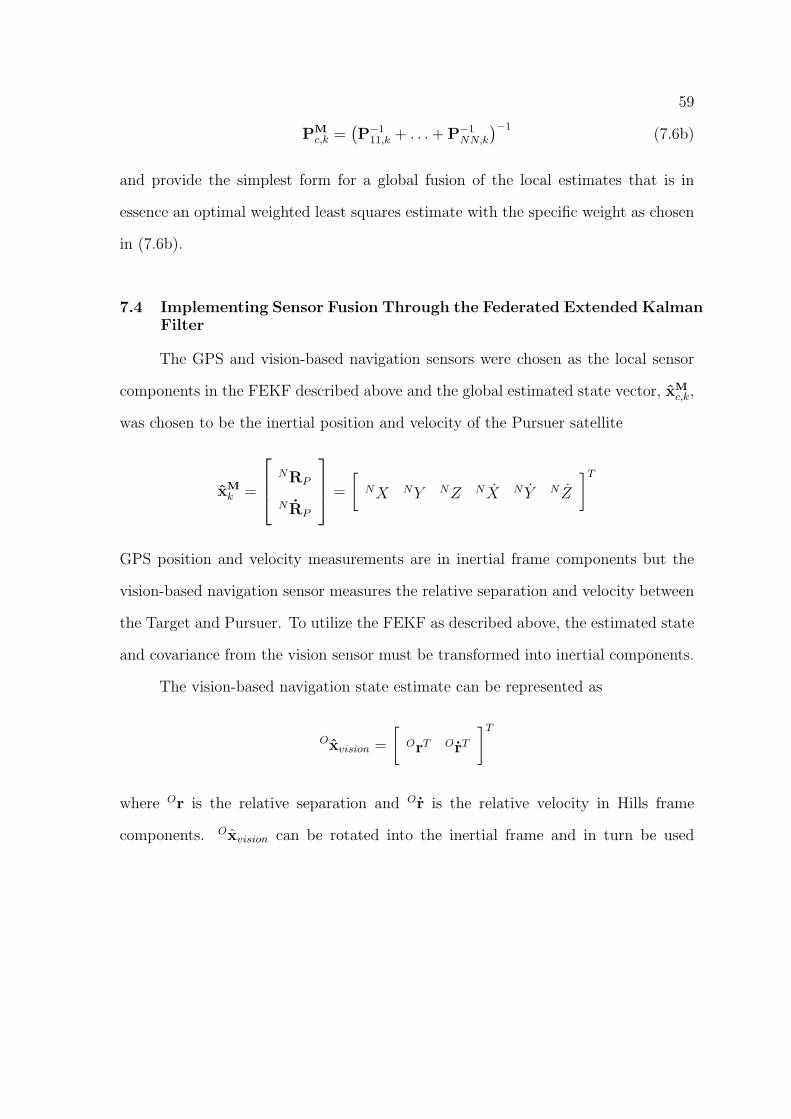
CHAPTER 7
MULTI-SENSOR FUSION
The previous chapters have described individual sensor systems that are used
for navigation and control in this thesis. Both the GPS and vision sensor systems
have advantages and disadvantages for navigation, specifically rendezvous, however,
it is possible to use multiple sensors in conjunction to improve estimation performance
and in turn improve the control performance. Use of multiple sensors in conjunction
to create a single global or master estimate of the desired state parameters is known
as sensor fusion and is the main focus of this thesis.
Sensor fusion is generally achieved through two means: a centralized filter or a
decentralized filter. The following chapter will describe the difference between these
two filter types, develop the algorithm for the decentralized filter, and apply that filter
to the GPS and vision sensors previously developed to create a global state estimate
in the form of a Federated Extended Kalman Filter.
7.1 Centralized Kalman Filter Architecture
A general centralized Kalman filter architecture is depicted in Figure 7.1. In
this setup, a series of independent local sensors provide uncorrelated measurements
(Y1, . . . ,YN) on some larger global system. The measurements from these sensors
can be fed to a conventional Kalman filter to obtain an optimal estimate of the
global state called a global or centralized Kalman filter. Although this global filter
can provide an optimal linear minimum-variance (LMV) solution to the estimation
problem, the large number of states in the global system often requires processing
54
55
data rates that cannot be maintained in practical real-time applications. For this
reason, and because smaller parallel structures can often provide improved failure
detection and correction, improved redundancy management, and lower costs for
system integration, there has been considerable recent interest in decentralized (or