Generic health modelling

55

CHAPTER 3

MULTI-STATE MODELLING OF DISEASE OCCURRENCE

3.1 SUMMARY Introduction This chapter describes a generic multi-state modelling approach to population health that addresses the effectiveness and efficiency of population health interventions. The objective of this approach is to function as a general frame of reference to be used when one addresses specific questions. Methods The main characteristic of such an approach is that it considers the main relationships between population health in terms of health states and flows between them. It includes both environmental and societal determinants in a dynamic and disease-specific way. This may include populations living with a low socio-economic status as well as those living at the highest known income levels. It may be used for analyses of population health in the past and in the future. This approach means a quantitative description of the disease epidemiology at the population level, taking into account the demonstrated confounding effects of the health determinants. There are many diseases and many intervention options; there are many ways to fall ill, many causes to die from, and a diversity of instances to actively intervene. There are many options to prevent people from falling ill, to improve recovery and the quality of survival of disease, and to avert premature mortality. Results This chapter has shown how disease and death can be described in a generic multi-state model and how health interventions might be effective. It shows the building blocks for a generic framework for population health. It distinguishes and defines macro- and micro-determinants and multiple disease states. Next, it describes the practical and pragmatic approach in the mathematical implementation, distinguishing various transition probabilities between disease states and a number of aggregate outcome measures. In addition, it summarises approaches to demonstrate the validation, calibration, and robustness of outcomes and structure of the generic framework. The generic modelling approach is used in a number of studies. Chapter 4 distinguishes single disease states for a number of diseases together. It quantifies the contribution of health determinants to mortality decline in India, Mexico, and The Netherlands. Then, the next chapter analyses the decline in stroke mortality (chapter 5) using a stroke model with multiple states. In the chapters 6 through 8, the contributions of the health interventions to reduce the burden of stroke and diabetes are evaluated. In these latter cases, the descriptions of large single disease multi-state models may not show some of the elements of the generic approach. This application of the principle of parsimony is under the assumption that the indicated macro-determinants, such as nutritional status and socio-economic status, and other disease states do not influence model outcomes or the final conclusions. Conclusion The modelling framework can be used to explore, to specify, and to analyse research and policy questions. This is both possible for use at the macro-level and to test more specific hypotheses in epidemiology, health economics, demography, and public health.

Chapter 3

56

Generic health modelling

57

3.2.GENERIC APPROACH TO MULTI-STATE HEALTH MODELLING Converging pathways in the health transition form the basis of the two postulates outlined in the preceding two chapters. These define population health by the presence of a specific pattern of health determinants and also distinguish slower and quicker roads to health. As formulated differently by Georfrey Rose: there is no biological reason why a population should not be as healthy as the best (Rose, 1992). These statements are the equivalent of the more technical hypothesis that the model is generic. This implies that the observed empirical pattern of population change and burden of disease can be attributed to the levels and interactions of population and health determinants. It implies that the approach can be used to assess populations on various geographical scales, for different time periods, and with different degrees of differentiation of determinants, age groups, disease classes, and health services. The population health macro-determinants represent those factors that influence the proximate health determinants. The selection of determinant categories is based on the evidence regarding their supposed quantitative importance throughout the health transition as reported in the literature. They are categorised in two groups: socio-economic determinants and environmental determinants. The two variables describing the socio-economic determinants are:

• Gross National Product (GNP) expressed in 1990 US-dollars. This parameter determines the available income per capita and the resources available for health services. Separate projections for the low-income countries are used in a distribution function to estimate the number of people below the absolute poverty line (World Bank, 1993);

• The female literacy level expressed as the fraction of the literate adult, female population. This parameter is computed as a delayed function of GNP and the Human Development Index (HDI) (UNDP, 1993-1995).

The variables describing the environmental determinants are: • Food supply expressed in kilocalories daily intake per person. Input scenarios on

the availability of food define the fraction of the population suffering from malnutrition. This fraction is calculated for the sub-populations that fall under the low socio-economic status categories (see below). These calculations are based on an empirical distribution function (FAO, 1987 & 1992);

• Safe water and sanitation access defined as the fraction of the population with proper access to safe drinking water and having sanitation, that falls under the low socio-economic status categories. In case of large discrepancies between the two parameters the safe drinking water coverage is chosen because this determinant is the most relevant of the two (Esrey et al., 1985, 1991);

Chapter 3

58

ENVIRONMENT

FERTILITY POPULATION

POLICIES

POPULATION DYNAMICS

MACRO HEALTH DETERMINANTS

REPRODUCTION POLICY

WATER POLICY

FOOD POLICY

HEALTH SERVICES

DRINKING WATER

DISEASE OCCURRENCE

DISEASE BURDEN POPULATION SIZE

FOOD

POPULATION HEALTH EFFECTS

SOCIO-ECONOMIC

INCOME LITERACY

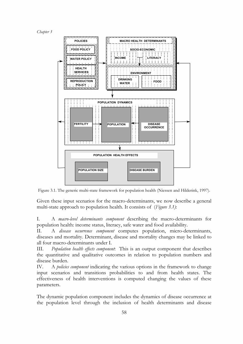
Figure 3.1. The generic multi-state framework for population health (Niessen and Hilderink, 1997).

Given these input scenarios for the macro-determinants, we now describe a general multi-state approach to population health. It consists of (Figure 3.1): I. A macro-level determinants component describing the macro-determinants for population health: income status, literacy, safe water and food availability. II. A disease occurrence component computes population, micro-determinants, diseases and mortality. Determinant, disease and mortality changes may be linked to all four macro-determinants under I. III. Population health effects component: This is an output component that describes the quantitative and qualitative outcomes in relation to population numbers and disease burden. IV. A policies component indicating the various options in the framework to change input scenarios and transitions probabilities to and from health states. The effectiveness of health interventions is computed changing the values of these parameters. The dynamic population component includes the dynamics of disease occurrence at the population level through the inclusion of health determinants and disease

Generic health modelling

59

categories. As said, the health determinants are linked to income and literacy changes, food and water availability and service expenditures per capita by service category. All health states are divided in age groups. The selection of the size of the age groups is determined by the epidemiology of disease of the three health transition stages. Group members may leave a state by age group because of ageing. In addition, in each age group for each health state group members may change towards another single- or multi-determinant category. In turn, this latter category may lead to single or multiple disease states. The likelihood of transition from healthy to diseased or transition between disease states or from one disease state to another, a probability, is independent from the preceding events and depends on age, sex, determinant type and disease status. The probabilities in the disease model are a function of nutritional status and the level of curative health services. The numbers of persons that remain in disease prevalence states determine the level of permanent disability associated with the particular disease. The disease burden attributed to a specific health determinant is calculated as life years lost because of mortality and weighted years lost because of disease. Additional outcomes can be calculated by adding specific components relating disease burden to additional economic impact like direct and indirect costs of illness (Drummond, 1986; Gold, 1987). The computed disease burden may influence, in a feedback loop, the health resources needed, but not their effectiveness. The population health model simulates the number of persons suffering from diseases and the number of deaths related to these diseases. The disease figures are used to estimate the disease burden in the population. The computed death figures determine the overall age- and sex-specific mortality rates. The core assumptions related to the model structure and dynamics are listed in Box 1. I. The use of large population categories (in defining age groups, determinant types, disease groups and service

categories) is justified in case of long term dynamics and population assessment at high aggregation levels (life expectancy, population size and total fertility levels) e.g. chapter 4. In the case of more specific research questions more detailed analysis is necessary (chapters 5-8).

II. There is a hierarchy in the causal contributions of health determinants. First level determinants are socio-economic and nutritional status. Next, depending on the level of these two, traditional risk factors have their effects.

III. Two economic status categories are used: above/below the internationally defined poverty line. Two nutritional status categories are used based on the availability of sufficient dietary kilocalories: above/below the basic metabolic rate by international standards.

IV. The contributions of each health determinant to the occurrence of disease and death can be quantified through corresponding relative risks, known from public health epidemiology.

V. The effect of health services can be modelled using a general effectiveness function. This function changes the modelled health determinants from a known minimum effect (based on data on subsistence health situations) to a maximum effect (from data from the healthiest populations).

VI.Change in mortality by disease group can be (almost) fully explained by 1) changes in broad and specific health determinants, affecting disease incidence and survival, and 2) the effect of preventive and curative services, affecting health determinants and disease survival, respectively.

VII.Parameter values from epidemiological surveys can be used in modelling population health if the survey setting is comparable to that of the involved populations e.g. population- or health-service-based.

Box 1: Core assumptions of the population health framework

Chapter 3

60

In the general framework, we define a number of health-related states by age group and by sex, influenced by health determinants. This will be described in detail in the next sections. The health state states are treated in a similar way as the overall population within the population and health model: inflows and outflows of the states combined with an initial value determine the contents of the state at a particular point in time. The flows concerning the disease processes are shown in the next sections. Ageing and mortality from residual causes are accounted for in all health states and are not included in the model equations. 3.3. MULTIPLE HEALTH DETERMINANTS

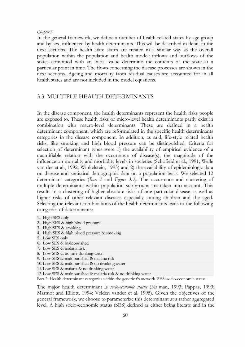
In the disease component, the health determinants represent the health risks people are exposed to. These health risks or micro-level health determinants partly exist in combination with macro-level determinants. These are defined in a health determinant component, which are reformulated in the specific health determinants categories in the disease component. In addition, as said, life-style related health risks, like smoking and high blood pressure can be distinguished. Criteria for selection of determinant types were 1) the availability of empirical evidence of a quantifiable relation with the occurrence of disease(s), the magnitude of the influence on mortality and morbidity levels in societies (Schofield et al., 1991; Walle van der et al., 1992; Winkelstein, 1993) and 2) the availability of epidemiologic data on disease and statistical demographic data on a population basis. We selected 12 determinant categories (Box 2 and Figure 3.3). The occurrence and clustering of multiple determinants within population sub-groups are taken into account. This results in a clustering of higher absolute risks of one particular disease as well as higher risks of other relevant diseases especially among children and the aged. Selecting the relevant combinations of the health determinants leads to the following categories of determinants: 1. High SES only 2. High SES & high blood pressure 3. High SES & smoking 4. High SES & high blood pressure & smoking 5. Low SES only 6. Low SES & malnourished 7. Low SES & malaria risk 8. Low SES & no safe drinking water 9. Low SES & malnourished & malaria risk 10. Low SES & malnourished & no drinking water 11. Low SES & malaria & no drinking water 12. Low SES & malnourished & malaria risk & no drinking water Box 2: Health determinant categories within the generic framework. SES: socio-economic status.

The major health determinant is socio-economic status (Najman, 1993; Pappas, 1993; Marmot and Elliott, 1994; Velden vander et al. 1995). Given the objectives of the general framework, we choose to parameterize this determinant at a rather aggregated level. A high socio-economic status (SES) defined as either being literate and in the

Generic health modelling

61

low-income group, or being in the high or middle-income categories (Caldwell, 1973-1993) and living above the poverty line, as defined by international criteria (Heerink, 1994; Moreland, 1984; World Bank, 1992-1994 and Lim Chong Yah, 1991). Low SES is defined as being of the low-income category and illiterate or living below the poverty line. Hence, the basic equation is, for each moment in time: high SES fraction = fraction high/mid income + fraction literate * (fraction low income - fraction poor) (4.1)

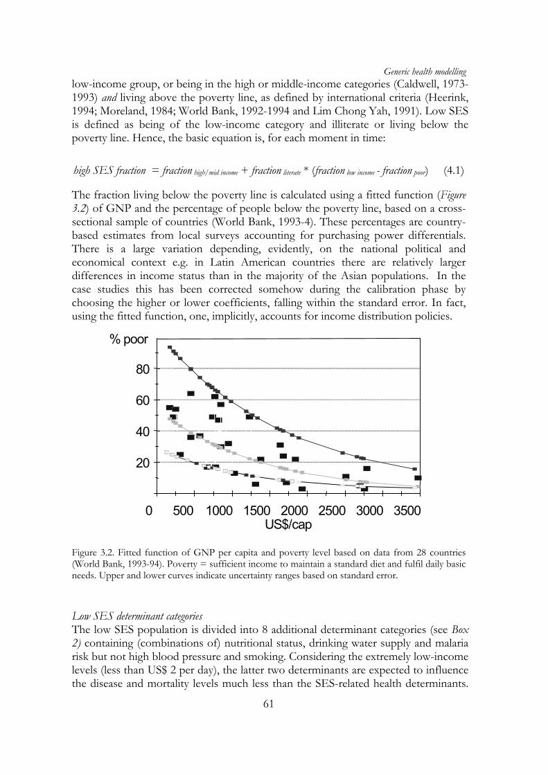
The fraction living below the poverty line is calculated using a fitted function (Figure 3.2) of GNP and the percentage of people below the poverty line, based on a cross-sectional sample of countries (World Bank, 1993-4). These percentages are country-based estimates from local surveys accounting for purchasing power differentials. There is a large variation depending, evidently, on the national political and economical context e.g. in Latin American countries there are relatively larger differences in income status than in the majority of the Asian populations. In the case studies this has been corrected somehow during the calibration phase by choosing the higher or lower coefficients, falling within the standard error. In fact, using the fitted function, one, implicitly, accounts for income distribution policies.

20

40

60

80

% poor

0 500 1000 1500 2000 2500 3000 3500 US$/cap

Figure 3.2. Fitted function of GNP per capita and poverty level based on data from 28 countries (World Bank, 1993-94). Poverty = sufficient income to maintain a standard diet and fulfil daily basic needs. Upper and lower curves indicate uncertainty ranges based on standard error.

Low SES determinant categories The low SES population is divided into 8 additional determinant categories (see Box 2) containing (combinations of) nutritional status, drinking water supply and malaria risk but not high blood pressure and smoking. Considering the extremely low-income levels (less than US$ 2 per day), the latter two determinants are expected to influence the disease and mortality levels much less than the SES-related health determinants.

Chapter 3

62

The most important low SES category is nutritional status (Binswanger and Landell, 1995; Pelletier, 1993-1995). Malnutrition prevalence is computed based on a function of the availability in kilocalories per capita daily food intake. Malnourished is defined as a lack of sufficient food intake in kilocalories i.e. less than 1.54 times the basic metabolic rate in kilocalories per day (1575 for adult males). Standards have been set by age, sex and body weight and also by pregnancy status. This distribution function is based on the empirically fitted relationship given by the FAO as reported in the fifth World Food Survey (1987). World food supplies and prevalence of malnutrition in low-income regions have been reassessed in 1992 (FAO, 1992). This resulted in adapted coefficients (see function below). In the module the percentage malnourished is calculated from the average food availability per capita as an input scenario. The fraction malnourished for each time step can be calculated as (Ashworth and Dowler, 1991):

))*31.4exp(*01.01(1

factorfoodfractionnourishedmal

+= (4.2)

In this equation the food factor is a factor that is obtained in a function depending on food availability and age- and sex-specific daily need of food. For pregnant women in age group 15-45 an additional need of 138 Kcal per day is taken into account. The additional data in relation to the occurrence of diseases are based on the available international literature (Crigg, 1989; Dreze and Sen, 1989; Kielman and McCord, 1978; Pelletier, 1993 & 1995; Pinstrop-Anderson et al., 1993; Pinstrop-Anderson and Pandya, 1995; Sachdev et al., 1992; Vella et al., 1994; Niessen & Hilderink, 1997b) Another important health determinant is access to safe drinking water. The provision of proper drinking water depends on the total public water supply investments. The population without public water supply and relying on private supply is regarded as having no access to safe drinking water and runs higher relative health risks of waterborne diseases. The input scenario for this parameter is based on international estimations on costs and economic growth (chapter 4, section 4.4). Sanitation facilities are included in these costs and are not considered to make an additional contribution in reducing the water-borne diseases. The independent preventive effect on disease occurrence seems very limited (Ahmed, 1994). The next health risk modelled related to SES is the presence of malaria mosquitoes carrying malaria parasites. The fraction of the population exposed to such a malaria risk is based on internationally standardized estimations (Martens et al., 1995). This fraction is, again, influenced by health policy through vector control programmes. The fraction of malaria-affected population is also a function of socio-economic development. High SES health determinants categories The high SES population is divided into those exposed to smoking or not and those having high blood pressure or not. Scenarios for these determinant categories are sex- and age-specific and based on empirical time series. Trends are extrapolated but still subject to health services effects i.e. preventive measures. It is assumed that

Generic health modelling

63

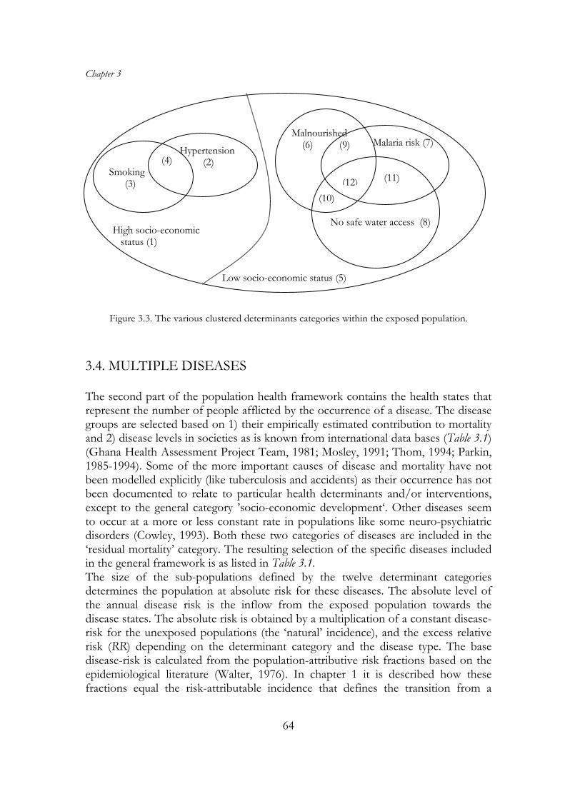
people who reach only this level of socio-economic development will be exposed to these two health risks. The input series for smoking levels are based on estimations of the tobacco production since 1900 (WRI, 1995). Although the occurrence of related health problems has been rising first in the sixties and seventies in Europe, the mortality figures are now rising worldwide although much more among men than among women (Peto, 1992; Bartecchi et al, 1994-1995; McKenzie et al,, 1994). Input data are based on existing survey data and reviews or existing models (Tunstall, 1994; Ruwaard et al., 1993; Niessen et al., 1993). The prevalence of smoking is increasing and reaching very high levels (up to 70-85%) in large areas of the world, especially in countries with low-income levels. There is a world smoking prevalence estimate by WHO of 52% for men and 10% for women and there are estimates for e.g. China of even 61% for men and 7% for women (Stanley, 1993). The relationship between smoking and a large number of diseases is clear and has been quantified (Jackson and Beaglohole, 1987; McGovern et al, 1992; Pearson et al., 1993). In case of mortality change, one often observes a change in health risk prevalence that changes disease incidence, but also a change in disease survival. There might be two types of independent changes, as a consequence of prevention interventions or an increase in survival due to curative activities (Farchi, 1984; Dobson, 1994; Bonneux et al. 1996). The potential health gain by reducing health risk prevalence is large (Gunning, 1989; Tsevat et al., 1991; Grover et al., 1994). The epidemiological input data used are based on existing surveys or existing models (Tunstall et al., 1991, Bonneux et al., 1994). The relationship between high blood pressure and cardio-vascular disease, ischemic heart disease or stroke, has also been quantified (Dyken, 1984; Klag et al., 1989; McGovern & Beaglehole, 1987; Casper et al., 1992; Whelton, 1994). There are also estimates of the potential health gain by treatment or prevention (Gunning-Schepers, 1989). Data are based on existing survey data, reviews or existing models (Tunstall et al., 1991, Niessen et al., 1993, Ruwaard et al., 1993). Combining health determinants The various combinations of the health determinants are depicted in Figure 3.3. Assumed is an independent occurrence of most categories except for the combination of malnutrition and no access to safe drinking water where a correlation/clustering factor of 1.1 is used. This figure proved to be the maximum possible still explaining empirical data (World Bank, 1993). In this way a clustering of health determinants among the populations with low economic status can be simulated. Criteria for selection of determinant types are 1) the empirical evidence based on the epidemiological literature on a quantifiable relation between the health determinant(s) and disease and mortality levels in societies ((Schofield et al., 1991); (Walle van de et al., 1992) and 2) the availability of population-based statistical data.

Chapter 3

64

Low socio-economic status (5)

High socio-economic status (1)

(10) (12)

Malaria risk (7)

(11)

No safe water access (8)

Hypertension (2)

Malnourished (6) (9)

(4) Smoking (3)

Figure 3.3. The various clustered determinants categories within the exposed population. 3.4. MULTIPLE DISEASES The second part of the population health framework contains the health states that represent the number of people afflicted by the occurrence of a disease. The disease groups are selected based on 1) their empirically estimated contribution to mortality and 2) disease levels in societies as is known from international data bases (Table 3.1) (Ghana Health Assessment Project Team, 1981; Mosley, 1991; Thom, 1994; Parkin, 1985-1994). Some of the more important causes of disease and mortality have not been modelled explicitly (like tuberculosis and accidents) as their occurrence has not been documented to relate to particular health determinants and/or interventions, except to the general category ’socio-economic development‘. Other diseases seem to occur at a more or less constant rate in populations like some neuro-psychiatric disorders (Cowley, 1993). Both these two categories of diseases are included in the ‘residual mortality’ category. The resulting selection of the specific diseases included in the general framework is as listed in Table 3.1. The size of the sub-populations defined by the twelve determinant categories determines the population at absolute risk for these diseases. The absolute level of the annual disease risk is the inflow from the exposed population towards the disease states. The absolute risk is obtained by a multiplication of a constant disease-risk for the unexposed populations (the ‘natural’ incidence), and the excess relative risk (RR) depending on the determinant category and the disease type. The base disease-risk is calculated from the population-attributive risk fractions based on the epidemiological literature (Walter, 1976). In chapter 1 it is described how these fractions equal the risk-attributable incidence that defines the transition from a

Generic health modelling

65

healthy state to a disease state. The RR represents the excess chance of getting a disease due to a specific health risk as compared to a reference population.

Category Specific disease Infectious and parasitic diseases Gastro-enteritis

Acute respiratory infections Measles Malaria

Maternal and perinatal diseases Prenatal mortality Maternal mortality

Cancers Lung Cancers All other cancers

Pulmonary disease Chronic obstructive pulmonary disease Circulatory and degenerative diseases Acute Infarctions

Chronic Heart Failure Stroke

Residual diseases Remaining mortality

Table 3.1. Disease categories within the generic model framework.

The values for these RRs are derived from the epidemiological literature (Ruwaard et al., 1994; Niessen et al, 1995). The estimates for malaria are based on the outcomes of a more detailed infectious disease model described elsewhere (Martens, 1995). The overall disease risk is determined by a base disease risk multiplied by the RR for the involved health determinant and involved disease, by age and sex. The basic equation for the disease determinants for all the determinant- and disease categories is as follows:

}10,...,2,1{disease},12,...,2,1{exposure},5,...,2,1{age},,{sex

)(population exposed*RR*risk diseasebase

)(risk disease

exposureage,sex,diseaseexposure,age,sex,diseaseage,sex,

disease exposure,age,sex,

∈∈∈∈∀

=

femalemalet

t

(4.3)

Here, the relative risk (RR) is a constant and the exposed population changes in time depending on births and deaths. The equation 4.4 defines the flow from the health determinant category to the disease states. It can be divided into three events (cp. Figure 1.4). The first is the event directly related to the absolute disease risk and is the case-fatality rate (CF), defined as the probability of dying during the acute episode of the disease. The levels of the case-fatality are age, sex and disease-specific. They are a function of the level of curative health service expenditures per capita. For each disease minimum and maximum values for the case-fatality are defined. These correspond to the lowest respectively highest known levels reported. A cure-effectiveness function determines the actual CF in between the extreme values:

Chapter 3

66

}10,...,2,1{diseases},5,...,2,1{age},,{sex)-( * )(

-=)(max

seasesex,age,dimin

seasesex,age,di

minseasesex,age,diseasesex,age,di

∈∈∈∀ femalemaleCFCFtesseffectivencure

CFtfractionCF

(4.4)

The second possible event is recovery within a year after becoming incident. Similar to the case-fatality, the level of recovery is determined by a cure-effectiveness function modified by the level of curative health service expenditure. The third event is entry into the disease state. They become chronically ill for the involved disease. The event is assumed irreversible. Next, there are two possibilities of leaving these disease states. The probability of dying is based on a overall base mortality risk and a disease-specific delayed mortality risk. This, late, surplus mortality risk is defined as the ‘late’ mortality risk. This fraction is likewise based on a minimum and maximum value and influenced by the effectiveness of curative health service expenditures. The second possibility of leaving the first disease state is getting another disease. Especially among the elderly but also among those with already respiratory disease this is frequent. In the general framework, ‘double-diseased’ states have been defined to include the eight most frequent combinations of chronic diseases. The events related to entry of this double diseased state are similar to getting a first disease: curing and dying are treated similarly, using the same functions and the same absolute values as for single diseased. The total disease-specific mortality figures by sex and age related to these eight diseases are obtained from the single and the double disease states. They are used to compute the survival of the population. The yearly ageing of the various sub-populations depends on the length of the age group and is roughly the inverse of that length in years (for example the ageing out of age group 0-5 is 1/5). Because of the non-uniform mortality distribution within the age groups, it is adapted to the distribution of people over the age group. This distribution is represented by the fraction of people surviving up to last year of the age group (in the example up to 5 years) divided by the length of the age period. Thus:

}5,...,2,1{},,{

)1(

)1()(

1,

,,

∈∈∀

−

−=

∑=

agefemalemalesex

proportionmortalitytotal

proportionmortalitytotaltageing

age

age

plengthgrou

i

iagesex

plengthgrouagesex

agesex

(4.5)

Here, ageing is the proportion of survivors in each age category, i.e. those that move on to the next age category. At last, total mortality is discussed. It consists of three components. The disease mortality fraction that is the mortality explained by the known disease epidemiology. This is based on the combinations of the various macro- and microdeterminants and the subsequent occurrence of disease and death. The second component is the maternal mortality fraction. This is calculated by a multiplication of the number of women of the ages between 15 and 45 years, the number of births and a maternal mortality risk based on the level of curative health care services. The third and last component is ‘residual mortality’. It is a, presumably biological, baseline level of

Generic health modelling

67

mortality, sex and age-specific, defined as the yearly mortality that can not be related to a particular cause. This mortality fraction is quantified using a golden standard life table. General outcome measures The most used general outcome measure that combines morbidity and mortality is disability-adjusted life years (DALYs) per thousand (World Bank, 1993). In this approach the time lost with disease, as acute or chronic case, is added to the time lost due to premature death as compared with the standard life table North (Murray, 1994). The weighing of the contribution of the different diseases to a loss of health is done separately for acute episodes and for chronic, prevalent, cases. The duration of an acute period depends on the disease: in general two weeks for infectious diseases and one month for chronic diseases. Chronic cases are counted as lasting a whole year. The time spent with disease is weighted by degree of related disability (Murray, 1994). We adapted this approach to calculate the disability-adjusted life expectancy (DALE) (Niessen en Hilderink, 1997). This computation accounts for both the loss of health through premature death as well as through disease. It is an aggregate measure. To calculate the number of life years for the computation of the DALE, the age of death is compared to an assumed estimated average upper limit of 82 years for men and 88 years for women at birth (Murray, 1994). The origin of the losses of health by category can be obtained from the population health framework. As it distinguished the 12 subpopulations by health determinant, the model records the relative contributions of each of the determinant categories to the occurrence of disease and death. In this way, the years lived and the average loss of health can be clustered into four categories, three related to health determinants, all measured in DALE years. These are: 1. the net healthy years lived per average lifetime and the loss of life years by three

clusters of health determinant: 2. loss due to high SES and life-style-related health determinants such as smoking, 3. loss due to low SES only, 4. loss due to environmental determinants, such as food, water and malaria in

combination with low SES. The occurrence of diseases is accounted for in the last three categories while the category ‘mortality from residual diseases’ is considered in a residual category. Now, after having defined the framework, the next section deals with the actual practical implementation of the model approach. 3.5. MODEL IMPLEMENTATION AND VALIDATION This section distinguishes first four concepts used in relation to model validation, relates examples from the five studies reported in the later chapters and describes validation of the generic framework.

Chapter 3

68

Validation is the process of establishing the adequacy of a given mathematical model in representing a given structure e.g. a disease process. There is a fundamental trade-off in testing a model for validation. Using a very stringent test one will need a large number of iterations in the development process and the final result will be too complex and yield limited insights. Using a simple test, most models may pass, poorly representing the involved problem, and turn out to be useless for solving the problem. Validation takes place during the whole of the process of model development. Constantly, one may seek arguments in support of the model but also for arguments to falsify the model. One may argue that one can accept a model, as long as it is impossible to falsify the model. Usually one starts with the simplest conceivable model and extends the model until it passes the validation tests. In the end, the modeller’s skill and intuition will have mostly determined the final trade-off between simplicity and adequate representation. Next, four closely related concepts are described: conceptual validation, calibration, external validation, and internal validation. They are described in the same order as in developing a model, although most may be used throughout the whole process. External validation usually is the most prominent feature in validation. There is a fifth concept, operational validity that is often distinguished. This is the appropriateness of the model to give answers to the raised question. The latter is part of a broader discussion on the general scientific approach and is not dealt with. 3.5.1. DEFINITIONS OF VALIDATION Conceptual validation Conceptual validation can be defined as the process to verify the used assumptions and concepts against existing scientific theories. This should be carried out in dialogue with experts in the involved field. It is the final judgement of the expert in the field that may lead either to acceptance or rejection of the chosen model approach. This validation is very much dependent on the problem and the domain involved. It is difficult to give general statements on this. Each disease, depending on the level of detail of the research question, will turn out to have its own characteristics to account for. Experts may differ in opinion. There are a number of structured ways to establish a consensus or to reach partial agreements e.g. the Delphi method. Empirical calibration Calibration can be defined as varying model input values in order to match model output values to empirical data from other sources. In the definition of parameters a model may remain close to empirical data and already established demographic and public health definitions. Still, given the model complexities, level of detail, and need for consistency, it often is necessary to adapt some input variables to be able to

Generic health modelling

69

reproduce existing data on population, disease, and mortality. When input parameters have large uncertainty ranges, calibration is used to limit these ranges. Example 1. A simple one-year state model for a single disease can describe the incidence, prevalence, and mortality from a disease. Fitting these in a consistent set reproducing the actual epidemiological data for these three parameters is a calibration process. An important assumption is that disease related events (remission, mortality) occur in the first year of the disease. This can be because of the biology of the disease, but more often, it is an assumption to just be able to describe the epidemiology for one particular year. It is usually true for acute diseases that either lead to death or recovery within the time span of one year. This often might not be the case for chronic diseases like cancers or cardiovascular conditions. The calibrated results give an adequate reproduction of empirical data for the involved year. The values and the used model structure do not necessarily describe the disease process in time, in a cohort manner, in an adequate way. This is not a problem as long as the objective is the description of the disease burden for a given calendar year. When one would like to assess the effects of interventions on the disease process, the simplified structure might become a source of inconsistencies. Example 2 Extending this model to a multi-state model would need adaptation in a two ways. It might need adaptation of the survival parameters to account for the additional disease stages or it might be an adaptation to account for the influence of other health determinants or diseases. When the number of states is limited and relatively basic mathematical functions are used, variable values also in this phase may be adapted in a calibration process to fit at least some external data. Variables whose values can be adapted during the calibration procedure are selected from the ‘free’ variables, i.e. those variables whose values are not exactly known or may have a range of plausible values. Formally, one could identify first, in a systematic multivariate sensitivity analysis, the most influential parameters. The variables that can be used for calibrating model outcomes can be the relative risks, hazard rates, or the residual mortality risk in each state. The intermediate parameters may not be used for calibration, as they may be a function of other parameters. Some parameters may, theoretically, be considered to represent the exact value, and cannot be varied, such as the baseline level or annual disease-specific mortality rates. The remaining parameter values may be varied within in stated range of e.g. ten percent to fit the empirical data. External validation Calibrated model variables can be compared with remaining empirical data for the similar study period and similar regional populations. This is called external validation of model outcomes. This is usually the core of the validation activities. Formally, one could express this in some ‘goodness-of-fit’ measure. These variables could be the crude output figures from a population model like total births, birth and death rate, life expectancy or population size. These can be compared to UN or other general statistical summary data. Additional parameters may be the same as listed in the previous section as long as they are not used for calibration: intervention

Chapter 3

70

costs, expenditure, effectiveness of interventions, relative risks, residual mortality risk. More specific figures to use for validation can be the actual computed life expectancy of high or average risk groups (like the malnourished), disease-free life expectancy, based or not based on increased general mortality risk (like stroke survival) or disease-free expectancy (e.g. stroke free life expectancy). Actually, one should be looking for as much external data as possible for external validation. This will depend very much on the state-of-the epidemiology in the particular field. Internal validation Once calibrated, the model is run and tested to compare its intermediate outputs for consistency and to other existing data from empirical surveys, models or estimates from expert groups. We define this as internal validation. Example 1 It is fundamental that all input population t figures should be accounted for in the model. This means that the population totals, including births can be traced in the distribution across the various disease and mortality states. Hence, the sum of the living and births together should be equal to the sum of susceptibles, diseased and dead in all time steps. When the flows between the states are not adequately accounted for this may turn out not to be the case i.e. one looses people during the next time steps or one has too large a number of centenarians. Example 2 Disease incidences and disease-specific mortalities are relatively difficult to quantify, especially at the more aggregated population level. One can test the consistency of the multi-state model values by eliminating the disease-specific states and calculating directly the excess total age and sex-specific mortality by risk category. This can be done e.g. with the disease-specific figures for the malnourished category computing average overall excess mortality by age and sex. For various health determinant categories, this will yield the age-specific, possibly also sex-specific, overall mortality risk (see below in Table 3.2). Example 3 Rapid changing in input values may or may not be reflected in model outcomes. Sometimes, an existing model may not adequately simulate dynamics of disease occurrence as it uses too large time-intervals. One can test a model by introducing, manually or systematically, sudden changes in model inputs to see the effects on outcomes. The acceleration in incidence increase, and concomitant mortality, of e.g. infectious disease may not be simulated through a model with large time steps. A basically similar example might be the sudden changes in births. These can not be simulated accurately due to the use of too large age groups of women of the fertile age. In case of a baby boom, like after a war or recession, may not be reflected in perinatal and infant mortality rates when one uses five-year age groups. Its effect may be ‘diluted’ over a period of 5 years (the size of the first age group).

Generic health modelling

71

3.5.2. VALIDATION OF THE GENERIC FRAMEWORK

In the study presented in chapter 4 we have used empirical data for historical calibration of the model outcomes for periods of several decades or longer. We extracted these data from four types of sources: • national and international data registrations as reported or made available,

summarised by different levels of aggregation (national, regional), • population-based epidemiological surveys as reported in the literature or as used

by other models by different levels of aggregation (national, regional), • clinic-based research as reported in the literature and • other surveys at the population level in the field of the social sciences. Mostly, we used the data as input for the population health model without further calculation, interpolation, or smoothing. As can be expected, one finds many different parameter values in the literature. Our selection is based on the criterion that the involved study population should be similar to the defined (sub-) population in the model. This means that they relate to e.g. the high or low SES categories of the health determinants and corresponding diseases. One important exception is the use of data on acute respiratory infections and diarrhoeal disease for the chosen values for disease determinants, relative risks, case fatality and late mortality by age group, sex, determinant category and disease group as well as for the literature sources (Niessen and Hilderink, 1997). Variables whose values can be adapted during the calibration procedure are selected from the free variables, i.e. those variables whose values are not exactly known or may have a range of plausible values. In a systematic multi-variate sensitivity analysis, the following parameters in the framework appeared to be most influential: • female literacy coverage, in correlation with GNP, • the percentage of people below the poverty line, • the absolute GNP levels, • the curative expenditure and the effectiveness function for intervention options, • relative risks, • base-risks for mortality. The first two parameters of this list are not used for calibration as they are assumed a function of GNP. The last parameter is considered to represent the biological lower limit to the age-specific risks of mortality and is not varied either. The remaining three parameter values were varied within in range of ten percent to fit the empirical demographical time series. Seven calibrated model outcomes compare with the empirical time series for the period 1900-1990: the human development index, total births, crude birth and death rate, life expectancy, and the resulting population size. During the process, within the population model, the estimated number of

Chapter 3

72

perinatal deaths had to be increased to fit the population time series. This was effectuated by including the newborn in the malnourished determinant category. Hence, the simulated number of total deaths exceeds the historical estimates. During computation this malnourished fraction may disappear as food availability improves and, consequently, perinatal mortality lowers. The acceleration in increase in population could not be reproduced more accurately due to the large age groups used. The steady drop in perinatal and infant mortality that has been observed shows only up as a relatively slow increase in population. This is due to ‘dilution’ over the period of the size of the first age group. Internal validation of the generic framework Once calibrated, the model is run and tested to compare some additional intermediate output to other existing data from empirical surveys. This is defined as internal validation and shows the consistency of the model values across the various level of the model. In the generic framework, two flows related to the disease states, disease incidence and disease-specific mortality are relatively difficult to quantify for many populations, especially at the aggregate population level. We tested the consistency of the model values by eliminating the disease-specific states and calculating directly the excess total age and sex-specific mortality by determinant category for the year 1990. When dividing these by the figures for corresponding reference categories, the high SES and low SES age and sex-specific mortality, one computes in fact ‘simulated’ relative risks, determinant-attributable figures on the excess risk of total mortality by age and sex category (Table 3.2). The top half of the table gives the values for the resulting relative risks for each health determinant category. The lower half of the Table 3.2 shows the corresponding values found in the literature. The table shows that the framework produces relative risks in the same order of magnitude as reported in empirical surveys. One can also observe an appropriate age-gradient in the low SES categories. The empirical relative risks for malnutrition is based on a large number of study populations throughout the world (Pelletier, 1995) and is in between the simulated values. This can be expected as malnutrition clusters with a number of other health determinants. The reported relative risks for lack of safe drinking water shows a large range, although we selected the values from the most rigid surveys (Esrey et al, 1985). Other ways to internally validate the model are possible but are not elaborated as they depend very much on the available external data. Computing mortality decline in different historical populations and at different scales can also test the model framework. If this turns out to be possible, this contributes to the structural validity of model dynamics and genericity. We used the model for three countries: India, Mexico, and The Netherlands (see for details chapter 4).

Generic health modelling

73

Determinant High SES BP NIC NIC

+ BP Low SES NUT MAL WAT

NUT+

MAL

NUT+

WAT

MAL+

WAT

NUT+WAT +MAL

age Men 1-14 1 1 1.6 1.9 1.9 2.5 2.2 2.8 3.1 15-44 1 1.0 2.4 2.6 1 1.2 2.2 1.3 2.5 1.5 2.6 2.8 45-64 1 1.3 2.3 2.5 1 1.1 1.6 1.1 1.7 1.2 1.7 1.8 65-75 1 1.3 2.1 2.3 1 1.0 1.3 1.1 1.3 1.1 1.3 1.4 75> 1 1.4 2.5 2.8 1 1.1 1.2 1.1 1.3 1.2 1.3 1.4 Women 1-14 1 1 1.6 1.9 1.9 2.5 2.2 2.8 3.1 15-44 1 1.0 2.6 2.6 1 1.2 2.0 1.2 2.2 1.4 2.3 2.5 45-64 1 1.1 1.9 2.0 1 1.1 1.5 1.1 1.6 1.2 1.6 1.7 65-75 1 1.3 1.8 2.1 1 1.0 1.3 1.0 1.4 1.1 1.4 1.4 75> 1 1.6 2.1 2.5 1 1.1 1.4 1.1 1.5 1.2 1.5 1.6

A. Simulated relative risks

Determinant BP NIC NIC + BP NUT MAL WAT

age Men 1-14 2.5 1.5-1.6 1.3-5.0 15-44 1.2 3.05 2.61 45-64 1.3 2.31 2.61 65-75 1.3* 2.09 2.61 75> 1.3* 1.54 NA Women 1-14 2.5 1.5-1.6 1.3-5.0 15-44 NA 2.69 NA 45-64 NA 2.52 NA 65-75 1.4* 2.00 NA 75> 1.4* 1.44 NA

B. Empirical relative risks.

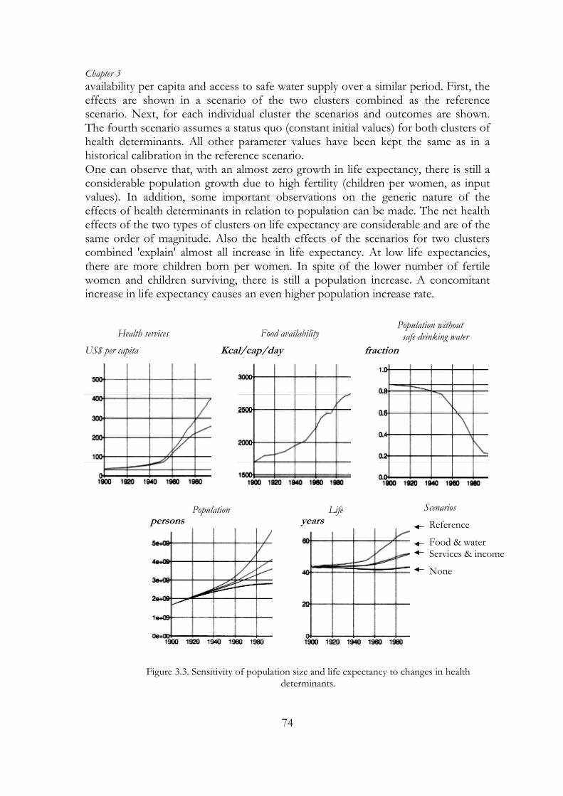
Table 3.2: Simulated (A) and empirical (B) relative risks for mortality by health determinant, age & sex. NA= not available. SES: Socio-economic status; BP = High blood pressure; NIC = smoking; NUT = malnutrition; MAL= Malaria exposure; WAT = no safe drinking water. Sources: High blood pressure: MRFIT-study (Marmot et al., 1994); * Chicago Heart Association Detection Project (Marmot and Elliot 1994); Smoking (Peto et al. 1992); High blood pressure & smoking: MRFIT-study; Malnutrition (Pelletier, 1995); Water risks: (Esrey, 1985 ); Malaria risk: Kisumu & Garki project (Najera et al., 1993). Sensitivity of outcomes to health determinants levels The robustness of a model to the input scenarios can be demonstrated by computing their relative quantitative effect on outcome measures. This indicates that the model equations and input values give an appropriate quantitative description of population health in relation to its determinants. Figure 3.3 shows some test results for population size and life expectancy to illustrate the robustness of the generic model version in relation to four scenarios for two clusters of determinants (Niessen and Hilderink, 1997b). A first cluster combines SES (national income, income status, income distributions and literacy) and health services level (prevention plus curative services). The second cluster includes food

Chapter 3

74

availability per capita and access to safe water supply over a similar period. First, the effects are shown in a scenario of the two clusters combined as the reference scenario. Next, for each individual cluster the scenarios and outcomes are shown. The fourth scenario assumes a status quo (constant initial values) for both clusters of health determinants. All other parameter values have been kept the same as in a historical calibration in the reference scenario. One can observe that, with an almost zero growth in life expectancy, there is still a considerable population growth due to high fertility (children per women, as input values). In addition, some important observations on the generic nature of the effects of health determinants in relation to population can be made. The net health effects of the two types of clusters on life expectancy are considerable and are of the same order of magnitude. Also the health effects of the scenarios for two clusters combined 'explain' almost all increase in life expectancy. At low life expectancies, there are more children born per women. In spite of the lower number of fertile women and children surviving, there is still a population increase. A concomitant increase in life expectancy causes an even higher population increase rate.

Scenarios

Reference

Food & water Services & income

None

Health services Population without safe drinking water

Population

fraction

Life

US$ per capita

years persons

Kcal/cap/day

Food availability

Figure 3.3. Sensitivity of population size and life expectancy to changes in health determinants.

Generic health modelling

75

3.6. CONCLUSION

This chapter describes the building blocks for a generic framework for population health. It distinguished and defines macro- and micro-determinants and multiple disease states. Next, it describes the practical and pragmatic approach in the mathematical implementation, distinguishing various transition probabilities between disease states and a number of aggregate outcome measures. In addition, it summarises approaches to demonstrate the validation, calibration and robustness of model outcomes and structure. The generic multi-state approach has been applied in studies in the next chapters. Chapter 4 distinguishes single disease states for a number of diseases together. It quantifies the contribution of health determinants to mortality decline in India, Mexico and The Netherlands as part of a larger programme at the Dutch National Institute. The next chapter analyses the decline in stroke mortality (chapter 5) using a multiple state model. Next, chapters 6 through 8 present the contributions of various health interventions to reduce the disease burden of stroke and diabetes. In these latter cases, the descriptions of the large single disease models do not show a lot of the elements from the generic approach. Here, the principle of parsimony rules: the assumption is that the excluded parameters, such as the determinants nutritional status, socio-economic status or specific health risk factors, as well as the presence of other diseases do not influence model outcomes nor the final conclusions.

Chapter 3

76

REFERENCES 1. Ahmed F, Clemens JD, Rao MR and Banik AK (1994): Family latrines and paediatric Shigellosis in rural Bangladesh: benefit or risk? Int J Epi 23 4 856-862. 2. Ashworth A and Dowler E: Child malnutrition. Chapter 8 in: Feacham RG and Jamison DT (eds) (1991): Disease and mortality in Sub-Saharan Africa. World Bank. Oxford UP. 3. Bairagi R and Chowdhury MK (1994): Socio-economic and anthropometric status, and mortality of young children in rural Bangladesh, Int J Epid 23 1179-1184. 4. Bartecchi CE, McKenzie TD and Schrier RW (1994): The human costs of tobacco use - part I; NEJM 330 907-12. 5. Bartlett A III, Paz de Bocaletti ME and Bocaletti MA (1993): Reducing perinatal mortality in developing countries: high risk management or improved labor management?, Hlth Pol Plan 8 4 360-8. 6. Binswanger HP and Landell Mills P (1995): World Bank’s strategy for reducing poverty and hunger - a report to the development community- 7. Black, R.R., Brown, K.H. and Becker, S. (1984). Malnutrition is a determining factor in diarrheal duration and severity but not incidence, among young children in a longitudinal study in Bangladesh. American Journal of Clinical Nutrition, 39: 87-94. 8. Bonneux L, Barendregt JJ, Meeter K et al. (1994): Estimating clinical morbidity due to ischemic heart disease and congestive heart failure: the future rise of heart failure: AJPH 84 20-25. 9. Bonneux L, van de Mheen PJ, Gunning-Schepers LJ, van der Maas PJ (1996): Did hypertension diminish in The Netherlands between 1974 and 1993? Ned Tijdschr Geneesk 140 2603-6. 10. Caldwell JC (1979): Education as a Factor in Mortality Decline: an examination of Nigeria data; Population Studies 1979 33 3 11. Caldwell JC (1993): Health Transition: the Cultural, Social and Behavioural Determinants of Health in the Third World; Soc Sci Med 1993 36 125-35, 12. Caldwell JC (1986): Routes to low morbidity in poor countries, Pop Dev Rev 1986 12 2. 13. Casper M, Wing S, Srogatz, Davis CE and Tyroler HA(1992): Anti-hypertensive treatment and US trends in stroke mortality - 1962-1980; Am J Public Health 12:1600-1608. 14. Cowley P and Wyatt RJ (1993): Schizophrenia and manic-depressive illness. Chapter 28 in: Jamison DT, Mosley WH, Measham AR and Bobadilla JL (eds): Disease control priorities in developing coun-tries. World Bank. Oxford Medical Publications, New York. 1993. 15. Crigg D (1989): The world food problem 1950-1980. Basic Blackwell 16. Dobson AJ (1994): Relationship between risks trends and disease trends, Ann Med 1994 26 67-71. 17. Dreze J and Sen A (1989): Hunger and public action. Clarendon Press, Oxford 18. Drummond MF (1987), Stoddart GL and Torrance GW: Methods for the economic evaluation of health care programmes. OUP. 19. Dyken ML, Wolf PA, Barnett HJM, Bergan JJ, Hass WK, Kannel WB, Kuller L, Kurtzke JF and Sundt TM (1984): Risk factors in stroke; Stroke 1984 15 1105-10. 20. Esrey SA, Feacham RG and Hughes JM: Interventions for the control of diarrhoeal disease among young children: improving water supplies and excreta disposal facilities, Bull WHO 1985 63 757-72. 21. Esrey SA, Pothas JB, Roberts L and Shiff C: Effects of improved water supply and sanitation on ascariasis, diarrhea, dracunculiasis, hookworm infection, schistosomiasis and trachoma; Bull. WHO 1991 69 609-621. 22. FAO- Food and Agriculture Organisation (1992): World food supplies and the prevalence of chronic undernutrition in developing regions as assessed in 1992. Statistical Analysis Office, Statistics Division, Economic and Social Policy Department, Rome. 23. FAO-Food and Agriculture Organization: The fifth world food survey m- 1985. Food and Agricultural Organization of the United Nations, Rome, Italy, 1987. 24. Farchi G: Spontaneous changes in risk factors and prediction of coronary heart disease; Preventive Med 1984;12:37-39. 25. Ghana Health Assessment Project Team: A Quantitative Method of Assessing the Health Impact of Different Diseases in Less Developed Countries (1981): Int J Epi 10(1):73-80.

Generic health modelling

77

26. Gold MR, Siegel, J.E., Russell, L.B., Weinstein, M.C.(1996): Cost-effectiveness in health and medicine. Oxford: Oxford University Press. 27. Graham WJ (1991): Maternal mortality: levels, trends and data deficiencies. Chapter 6 in: Feacham RG and Jamison DT (eds): Disease and mortality in Sub-Saharan Africa. World Bank. Oxford UP. 28. Grover SA, Gray-Donal K, Joseph L, Abrahamowics and Coupal L (1994): Life expectancy following dietary modification or smoking cessation; Arch Intern Med 154:1697-1704. 29. Gunning-Schepers LJ (1989): The health benefits of prevention; Health Policy 12:93A-129A. 30. Heerink N (1994): Population growth, income distribution, and economic development. Theory, methodology and empirical results. Population Economics Series. Springer Verlag. 31. Jackson R and Beaglehole R (1987): Trends in dietary fat and cigarette smoking and the decline in coronary heart disease in New Zealand; Int J Epi 16(3):377-382. 32. Kielmann, A.A. and McCord, C. (1978): Weight for age as an index of risk of death in children. Lancet 1: 1247-1250. 33. Klag MJ, Whelton PK and Seidler AJ (1989): Decline in US stroke mortality: demographic trends and antihypertensive treatment; Stroke 20:14-21. 34. Lim Chong-Yah (1991): Development and underdevelopment. Longman. Singapore. 35. Marmot M and Elliott P (1994): Coronary health disease epidemiology - from aetiology to public health. OUP. New York. 36. Martens WJM, Niessen LW, Rotmans J, Jetten TH and McMichael AJ (1995): Potential impact of global climate change on malaria risk, Environmental Health Perspectives 103 5 458-464. 37. McGovern PG, Burke GL, Sprfka JM, Xue S and Blackburn H: Trends in mortality, morbidity and risk-factor levels for stroke from 1960 to 1990: the Minnesota Heart Survey; JAMA 268:753-9. 38. McKenzie TD, Bartecchi CE and Schrier RW (1994): The human costs of tobacco use - part II; N Eng J Med 330:975-980. 39. Moreland S (1984): Population, development and income distribution - a modelling approach. ILO. St.Martin’s Press. New York. 40. Mosley WH and Cowley P (1991): The challenge of world health, Population Bulletin 46 :2-39 41. Murray CJL and Lopez AD (1994): Quantifying disability: data, methods and results; Bull WHO 72: 447-80. 42. Najera JA, Liese BH and Hammer J (1993): Malaria. Chapter 13 in: Jamison DT, Mosley WH, Measham AR and Bobadilla JL (eds): Disease control priorities in developing countries. World Bank. Oxford Medical Publications, New York. 43. Najman JM (1993): Health and Poverty: Past, Present and Prospects for the Future, Soc Sci Med 36 157-66. 44. Niessen LW and Hilderink HBM (1997b): Roads to health – modelling the health transition. RIVM-report. Centre for Public Health Forecasting. 45. Niessen LW and Hilderink HBM (1997): The population and health model. Ch 4 in: Rotmans J and De Vries: Perspectives on global change: the TARGETS approach. Cambridge UP. ISBN 0 521 62176. 46. Niessen LW, Barendregt JJ, Bonneux L and Koudstaal PJ (1993): Stroke trends in an aging population; Stroke 24:931-939. 47. Pappas G, Queen S, Hadden W and Fisher G (1993): The increasing disparity in mortality rates between socio-economic groups in the United States, 1960 and 1986, N Engl J Med 329 103-9. 48. Parkin DM, Pisani P and Ferlay J (1993): Estimates of the worldwide incidence of eighteen major cancers in 1985, Int J Cancer 54 594-606. 49. Parkin DM (1994): Cancer in Developing Countries. In: Doll R, Fraumeni JF jr. and Muir CS: Trends in Cancer Incidence and Mortality; Cold Spring Harbor Lab Press. 50. Pearson TA, Jamison DT and Trejo-Gutierres J (1993): Cardiovascular disease. Chapter 23 in: Jamison DT, Mosley WH, Measham AR and Bobadilla JL (eds): Disease control priorities in develo-ping countries. World Bank. Oxford Medical Publications, New York. 51. Pelletier DL, Frongillo EA and Habicht JP (1993). Epidemiological evidence for a potentiating effect of malnutrition on child mortality. American Journal of Public Health, 83(8): 1130-1133. 52. Pelletier DL, Frongillo EA Schroeder DG and Habicht JP (1995): The effects of malnutrition on child mortality in developing countries, Bull WHO 73 443-448.

Chapter 3 53. Peto R, Lopez AD, Boreham J, Thun M and Heath C (1992): Mortality from tobacco in developing countries: indirect estimation from national vital statistics; Lancet 339;1268-78. 54. Peto R. Lopez AD, Boreham J, Thun M and Heath C (1994): Mortality from smoking in developed countries 1950-2000 - indirect estimates from National Vital Statistics. WHO/Imperial Cancer Research Fund. OUP. 55. Pinstrop-Andersen P and Pandya-Lorch R (1995): Alleviating poverty, intensifying agriculture and effectively managing natural resources. Food, Agriculture and the Environment Discussion Paper. International Food Policy Research Institute, Washington. 56. Pinstrop-Anderson P, Burger S, Habicht JP and Peterson K (1993): Protein-energy malnutrition. Chapter 18 in: Jamison DT, Mosley WH, Measham AR and Bobadilla JL (eds): Disease control priorities in developing countries. Oxford Publications, New York. 57. Rose G (1992): The Strategy of Preventive Medicine. Oxford Medical Publications. OUP. 58. Ruwaard D, Kramers PGN, Berg Jetts van de A and Achterberg PW (eds) (1994): Public Health Status and Forecast: - the health status of the Dutch population over the period 1950-2010 SDU, The Hague. 59. Sachdev HPS, Stayanarayana L , Kumar S and Puri K (1992): Classification of nutritional status as ‘Z score’ or per cent of reference median - Does it alter mortality prediction in malnourished children?, Int J Epid 21 5 916-921. 60. Sai FT and Nassim J (1991): Mortality in Sub-Saharan Africa: an overview. Chapter 2 in: Feacham RG and Jamison DT (eds): (Disease and mortality in Sub-Saharan Africa. World Bank. Oxford UP. 61. Schofield R, Reher D and Bideau (1991): The decline of mortality in Europe. International Studies in Demography. Clarendon Press. Oxford 62. Stanley K (1993): Control of tobacco production and use. Appendix A in: Jamison DT, Mosley WH, Measham AR and Bobadilla JL (eds): Disease control priorities in developing countries.. Oxford Publications, New York. 63. Thom TJ and Epstein FH (1994): Heart disease, cancer, and stroke mortality trends and their interrelations; Circulation 90:574-582. 64. Tsevat J, Weinstein MC, Williams LW, Tosteson ANA and Goldman L (1991): Expected gains in life expectancy from various coronary heart disease risk factor modifications; Circulation 83: 1194-201. 65. Tunstall H, Kuulasmaa K, Amouyei P, Arveiler D, Rjakangas AM and Pajak A (1994): Myocardial infarction and coronary deaths in the WHO MONICA project - registration procedures, event rates, and case-fatality rates in 38 populations from 21 countries in four continents; Circulation 90:583-612. 66. UNDP- (1993-95) UN Development Programme: Human Development Report. Oxford UP. 67. UNEP (1997): Global Environmental Outlook, New York, Oxford UP. 68. Walle vander E, Pison G and Sala-Diakanda M (1992): Mortality and society in Sub-Saharan Africa. International Studies in Demography. Clarendon Press. Oxford 69. Walter SD (1976): The estimation and interpretation of attributive risk in health research; Biometrics 32:829-849. 70. Weinstein MC, Coxson PG, Williams LW, Pass TM, Stason WB, Goldman L (1987): Forecasting coronary heart disease incidence, mortality and cost: coronary heart policy model, AJPH 77 1417-26. 71. Weinstein MC (1988): Methodological issues in policy modelling for cardiovascular disease, J Am Coll Cardiol 14 38A-43A 72. Whelton PK (1994): Epidemiology of hypertension, Lancet 344 101-106 73. Whitmore TM, Turner BL II, Johnson DL, Kates RW and Gottschang TR (1990): Long-term population change. Ch. 2 in: Turner BL II, Clark WC, Kates RW, Matthews JT and Meyer WB: The earth transformed by global and regional change over the past 300 years. Cambridge UP. 74. World Hypertension League (1995): Economics of hypertension control, Bull WHO 73 417-24. 75. Winkelstein W (1993): Determinants of worldwide health, Am J Public Health 82 931-2. 76. World Bank (1993): Investing in Health - World Development Report. Oxford UP, New York. 77. WRI (World Resources Institute) (1995): World Resources 1995. Oxford UP, New York.

78