HAL Id: hal-01518088 https://hal-mines-paristech.archives-ouvertes.fr/hal-01518088 Submitted on 11 Jan 2018 HAL is a multi-disciplinary open access archive for the deposit and dissemination of sci- entific research documents, whether they are pub- lished or not. The documents may come from teaching and research institutions in France or abroad, or from public or private research centers. L’archive ouverte pluridisciplinaire HAL, est destinée au dépôt et à la diffusion de documents scientifiques de niveau recherche, publiés ou non, émanant des établissements d’enseignement et de recherche français ou étrangers, des laboratoires publics ou privés. Distributed under a Creative Commons Attribution| 4.0 International License Multiconfiguration electromagnetic induction survey for paleochannel internal structure imaging: a case study in the alluvial plain of the River Seine, France Fayçal Rejiba, Cyril Schamper, Antoine Chevalier, Benoit Deleplancque, Gaghik Hovhannissian, Thiesson Julien, Pierre Weill To cite this version: Fayçal Rejiba, Cyril Schamper, Antoine Chevalier, Benoit Deleplancque, Gaghik Hovhannissian, et al.. Multiconfiguration electromagnetic induction survey for paleochannel internal structure imaging: a case study in the alluvial plain of the River Seine, France. Hydrology and Earth System Sciences, European Geosciences Union, 2018, 22 (1), pp.159-170. 10.5194/hess-22-159-2018. hal-01518088
Transcript
HAL Id: hal-01518088https://hal-mines-paristech.archives-ouvertes.fr/hal-01518088
Submitted on 11 Jan 2018
HAL is a multi-disciplinary open accessarchive for the deposit and dissemination of sci-entific research documents, whether they are pub-lished or not. The documents may come fromteaching and research institutions in France orabroad, or from public or private research centers.
L’archive ouverte pluridisciplinaire HAL, estdestinée au dépôt et à la diffusion de documentsscientifiques de niveau recherche, publiés ou non,émanant des établissements d’enseignement et derecherche français ou étrangers, des laboratoirespublics ou privés.
Distributed under a Creative Commons Attribution| 4.0 International License
Multiconfiguration electromagnetic induction survey forpaleochannel internal structure imaging: a case study in
the alluvial plain of the River Seine, FranceFayçal Rejiba, Cyril Schamper, Antoine Chevalier, Benoit Deleplancque,
Gaghik Hovhannissian, Thiesson Julien, Pierre Weill
To cite this version:Fayçal Rejiba, Cyril Schamper, Antoine Chevalier, Benoit Deleplancque, Gaghik Hovhannissian, etal.. Multiconfiguration electromagnetic induction survey for paleochannel internal structure imaging:a case study in the alluvial plain of the River Seine, France. Hydrology and Earth System Sciences,European Geosciences Union, 2018, 22 (1), pp.159-170. �10.5194/hess-22-159-2018�. �hal-01518088�
Multiconfiguration electromagnetic induction survey forpaleochannel internal structure imaging: a case study inthe alluvial plain of the River Seine, FranceFayçal Rejiba1,a, Cyril Schamper1, Antoine Chevalier1, Benoit Deleplancque2, Gaghik Hovhannissian3,Julien Thiesson1, and Pierre Weill41Sorbonne Université – UPMC Univ Paris 06, CNRS, UMR 7619 METIS, Paris, France2UMR CNRS 7423 – Ecole Polytechnique de l’Université François Rabelais de Tours,35 allée Ferdinand de Lesseps, 37200 Tours, France3North Delegation of the Institute of Research for Development (IRD), UMR 242 iEES Paris (Institute of Ecology andEnvironmental Sciences), IRD/CNRS/UPMC/INRA/UPEC/Univ. Paris Diderot, 32 av. H. Varagnat, 93143 Bondy, France4Normandie Univ, UNICAEN, UNIROUEN CNRS, Morphodynamique Continentale et Côtière, 14000 Caen, Franceanow at: Normandie Univ, UNICAEN, UNIROUEN CNRS, Morphodynamique Continentaleet Côtière, 14000 Caen, France
Received: 17 February 2017 – Discussion started: 10 April 2017Revised: 2 November 2017 – Accepted: 18 November 2017 – Published: 10 January 2018
Abstract. The La Bassée floodplain area is a large ground-water reservoir controlling most of the water exchanged be-tween local aquifers and hydrographic networks within theSeine River basin (France). Preferential flows depend essen-tially on the heterogeneity of alluvial plain infilling, whosecharacteristics are strongly influenced by the presence ofmud plugs (paleomeander clayey infilling). These mud plugsstrongly contrast with the coarse sand material that composesmost of the alluvial plain, and can create permeability barri-ers to groundwater flows. A detailed knowledge of the globaland internal geometry of such paleomeanders can thus leadto a comprehensive understanding of the long-term hydroge-ological processes of the alluvial plain. A geophysical surveybased on the use of electromagnetic induction was performedon a wide paleomeander, situated close to the city of Nogent-sur-Seine in France. In the present study we assess the ad-vantages of combining several spatial offsets, together withboth vertical and horizontal dipole orientations (six apparentconductivities), thereby mapping not only the spatial distri-bution of the paleomeander derived from lidar data but alsoits vertical extent and internal variability.
1 Introduction
Dipolar source electromagnetic induction (EMI) techniquesare frequently used for critical zone mapping, which can beapplied to the delineation of shallow heterogeneities, therebyimproving conceptual models used to explain the processesaffecting a wide range of sedimentary environments. Thismapping technique is very effective for environments inwhich the spatial structure has strongly contrasted electro-magnetic (EM) properties – especially that of interpretedelectrical conductivity (EC).
Since the seminal work of Rhoades et al. (1976) much re-search has been conducted to link the petrophysical and hy-drodynamic soil properties to the apparent electrical conduc-tivity (ECa). ECa is affected by numerous parameters (Fried-man, 2005) whose major ones can be separated into three cat-egories: (1) the bulk soil properties (porosity, water content,structure), (2) the type of solid particle (geometry, distribu-tion and cation exchange capacity) mainly related to the claycontent, and (3) environmental factors (EC of water, temper-ature, etc.). The clay infilling of paleochannels and the depo-sition of alternate layers of conductive (clayey) and resistive(sandy) material in alluvial plain systems are examples of
Published by Copernicus Publications on behalf of the European Geosciences Union.
160 F. Rejiba et al.: Geophysical investigations of a paleochannel
natural geophysical processes having contrasting EM prop-erties.
EMI measurements have previously been applied to theimaging of conductive fine-grained paleomeander infilling,produced by meander neck cutoff or river avulsion, whichcan form permeability barriers with complex geometries (e.g.Miall, 1988; Fitterman et al., 1991; Jordan and Prior, 1992;De Smedt et al., 2011). In addition to providing detailed lo-cal information on alluvial plain heterogeneities, which canbe applied to the study of aquifer–river exchanges (Flipo etal., 2014), the estimation of the geometry of the Seine Riverpaleochannels can provide valuable insight into its paleohy-drology, as well as physical transformations resulting fromclimatic fluctuations during the Late Quaternary.
EMI devices are increasingly used for a large number ofnear-surface geophysical applications, as a consequence oftheir ability to produce mapping of ECa over extended ar-eas and at different depths. The main issue of EMI con-cerns the quantitative mapping of the vertical variations ofEC, obtained after multilayer inversion of ECa, becauseof the limited number of measurements at different depths(i.e. source–receiver offsets). Despite the spreading use ofmultiple-frequency and multiple-coil EMI instruments com-pared to the classic twin-coil configuration, a way to over-come this issue is, at least to constrain, and at best to cali-brate multilayer inversion of EMI measurements against ERI(electrical resistivity imagery) profiling. A very large body ofscientific literature has been published on the study and useof near-surface electromagnetic geophysics, especially in thefrequency domain, as described by Everett (2012).
By design, an EMI system energizes a transmitter coilwith a monochromatic oscillating current, and the oscillat-ing magnetic field produced by this current induces an os-cillating voltage response in the receiver coil. The voltageresponse measured in the absence of any conductive struc-ture is used as a standard reference. However, the magneticfield oscillations are distorted by the presence of nearby con-ductive structures, such that the voltage signal induced inthe receiver coil experiences a shift in amplitude and phasewith respect to that observed in the standard reference. Thisshift can be conveniently represented by a complex num-ber, comprising quadrature (or imaginary) and in-phase (orreal) components, which can be interpreted in terms of ECa(from the quadrature or out-of-phase part) and depth of inves-tigation (DOI) (Huang, 2005). A comprehensive and moredetailed description of the EMI principles can be found inNabighian (1988a, b).
Although EMI systems were initially used as mappingtools, and were designed to measure the lateral variabilityof EC associated with a single DOI, the measurements theyprovide are now generally interpreted to provide informationas a function of depth, albeit down to only relatively shal-low depths. This interpretation relies on the fact that, for agiven soil model, one specific DOI is defined by four de-vice setup parameters: (1) the offset between the transmit-
ter and receiver magnetic dipole, (2) the orientation of thedipole pair, (3) the frequency of the transmitter current oscil-lations, and (4) the instrument height above the ground. AnEMI survey during which at least one of these parameters isvaried can thus be used to resolve depth-related variations ofEC. This distribution can be retrieved by solving an inverseproblem, which is derived from a large number of applica-tions (e.g. Tabbagh, 1986; Nabighian, 1988b; Spies, 1989;Schamper et al., 2012).
The physical model used in the inversion procedure mustbe suitably adapted to the electromagnetic properties of thesurveyed ground. In the case of a medium characterized bytypical conductive properties (e.g. low, non-ferromagneticmaterials), at a low induction number the quadrature re-sponse is interpreted in terms of the apparent ground resistiv-ity, which to a first-order approximation varies linearly withthe quadrature response (McNeill, 1980). In a resistive (EMeffects other than induction become non negligible) or highlyconductive (low-induction number assumption is no longervalid) environment, such as that mapped in the present study,the EMI recordings, in particular their in-phase component,must be interpreted within the specific measurement context.One must then take into account, in addition to the EC, themagnetic susceptibility and viscosity, as well as the dielec-tric permittivity of the local environment, especially if this isresistive (e.g. Simon et al., 2015; Benech et al., 2016).
The present study focuses on the La Bassée alluvial plain,a zone located in the southern part of the Seine Basin, 2 kmto the west of Nogent-sur-Seine (France). The geophysicalcampaign was performed during 3 days of good weather inJune during a low-water period. The use of geophysical ex-ploration for this investigation is of significant importance,since it should pave the way for the paleohydrological re-construction of the Seine River (estimation of its transversalgeometry and paleo-discharge).
The aim of this study is to delineate the geometry of a pa-leochannel (i.e. its thickness and width), using a state-of-the-art 1-D inversion routine applied to EMI ECa measurements.The inverted data consist in a set of EMI measurements im-plemented with (1) three different offsets, and (2) for twodipole configurations: horizontal (HCP) and vertical (VCP).
Following a description of the study area, we present thetechnique used to calibrate the EMI measurements, whichrelies on reference ERI (electrical resistivity imaging) mea-surements and an auger sounding profile. The EMI inver-sion is then constrained to limit the solution space to im-ages that are consistent with the observations provided bythe ERI and auger soundings. To this end, a local three-layermodel is derived with fixed conductivities, and is then intro-duced into the inversion routine for each position of the sur-veyed area. The thicknesses of the soil and conductive filling,corresponding to the presumed paleochannel, are determinedthrough the use of an inversion algorithm.
F. Rejiba et al.: Geophysical investigations of a paleochannel 161
Figure 1. Maps of the Seine catchment (a) and the Bassée alluvialplain (b).
2 Description of the study area
The study site is located within a portion of the Seine Riveralluvial plain (locally named “Bassée”), approximately onehundred kilometres upstream of Paris (France), between theconfluence of the Seine and Aube rivers to the northeast, andthe confluence of the Seine and Yonne rivers to the southwest(Fig. 1). This 60 km long, 4 km wide alluvial plain constitutesa heterogeneous sedimentary environment, resulting from thedevelopment of the Seine River during the Middle and LateQuaternary.
Cartographic studies of this area have been carried out inthe past, using geomorphological and sedimentological tech-niques (Mégnien, 1965; Caillol et al., 1977; Mordant, 1992;Berger et al., 1995; Deleplancque, 2016), thus allowing thebroad-scale distribution and chronology of the location of themain Middle and Late Quaternary alluvial sheets to be esti-mated.
In addition, the French Geological Survey (BRGM) hascompiled a database of more than 500 soundings, which areuniformly distributed over the Bassée alluvial plain, and mostof which reached the Cretaceous chalky substrate. A detailed
Figure 2. Lidar map of the study area, showing the contemporarylocation of the Seine River, together with the narrow and wide pa-leochannel interpretations.
analysis and interpretation of this database has allowed thesubstratum morphology to be reconstructed, the alluvial in-filling thickness to be evaluated, and a preliminary quantita-tive analysis of the sedimentary facies distribution to be de-termined (Deleplancque, 2016). The maximum thickness ofthe alluvial infilling is thus known to lie between 6 and 8 m.
Geophysical investigations of gravel pits (after removalof the conductive topsoil) were carried out using ground-penetrating radar (Deleplancque, 2016), and have con-tributed to the characterization of the sedimentary contrastof the sand bar architecture, between the Weichselian andHolocene deposits. The Weichselian deposits are typicalof braided fluvial systems, with fluvial bars of moderateextent (< 50 m) truncated by large erosional surfaces. Thethickness of the preserved braid bars rarely exceeds 1.5 m.The Holocene architecture is associated mainly with single-channel meandering fluvial systems, characterized by thickpoint-bar deposits (> 4 m) with a lateral extent of several hun-dred metres, sometimes interrupted by clayey paleochannelinfillings. Traces of small sinuous channels, probably usingthe paths of former Weichseilian braided channels, are alsoidentified at the edge of the alluvial plain.
Aerial photography and a lidar (laser detection and rang-ing) topographic survey (Fig. 2) have been used to character-ize the paleochannel plan-view morphologies (style, width,meander wavelength), of the most recent (Holocene) me-andering alluvial sheets in this area (Deleplancque, 2016).These measurements were complemented by auger sound-ings and 14C dating of organic debris or bulk sediment (peat),in order to determine a time frame for the development of theSeine meanders and to allow these changes to be comparedwith other regional studies (e.g. Antoine et al., 2003; Pastreet al., 2003). The paleochannel investigated in this study is
162 F. Rejiba et al.: Geophysical investigations of a paleochannel
Figure 3. Map of the surveyed area, showing the locations of theVCP (red) and HCP (white) measurements (GPS issues explain theholes within the lines). The reference (ERI) profile, recorded witha Wenner–Schlumberger configuration using 1 m electrode spacingbetween 0 and 350 m, and a 0.5 m electrode spacing between 350and 401.5 m, is indicated by the yellow line. As green dots, the lo-cations of the hand auger drillings.
located 2 km to the southwest of Nogent-sur-Seine (coveredby a grassy meadow) and is characterized by larger dimen-sions than the present-day Seine River. Its width is estimatedto lie between 150 and 300 m, with a meander wavelengthbetween 2 and 3 km. According to the alluvial sheet analy-sis and the dating of organic material in the mud plug of theabandoned meander, it is very likely that this paleochannelwas active between the Late Glacial and Preoboreal periods(Deleplancque, 2016).
3 Field survey and measurement setup
The survey coordinates were determined through the use ofa lidar map (Deleplancque, 2016), combined with the anal-ysis of a series of auger soundings made along a referencetransect of almost 400 m in length (Figs. 2 and 3). The lat-eral extent of the meander was delineated using an EMI sys-tem (CMD explorer) produced by GF Instruments s.r.o., withnon-regular gridding and non-perfect overlapping inside thesame area.
3.1 ERI and hand auger soundings results
A total of 13 hand auger soundings down to a maximumdepth of 2.4 m (Fig. 4) were made along the reference pro-file. Some of these soundings did not reach the base of thepaleomeander mud plug (clay–gravel transition), suggest-ing that the maximum depth of the paleomeander is greaterthan 2.4 m. The auger soundings revealed the presence of
two main units. The uppermost unit is comprised of topsoil,which overlies a layer of loam containing a significant pro-portion of gravel and sand in the eastern part of the referenceprofile. A clayey layer, the bottom of which was not reachedin the deepest portion of the paleochannel, is situated belowthis unit. In some soundings, the clayey facies contains layersof peat (PTA, 04, 05, 06, 08, and 09, in Fig. 4).
The identification of the Holocene clay infilling along thisreference profile was confirmed by measuring several andoverlapping ERI profiles (24 m common), along the refer-ence transect. For this, a Wenner–Schlumberger array wasselected, with 48 electrodes positioned at a 1 m spacing forthe first 340 m, and a 0.5 m spacing thereafter.
The ERI cross section (Fig. 5) is produced using a datasetof more than 5000 measurements. A Wenner–Schlumbergerreciprocal array was used, which provides a good compro-mise between lateral and depth sensitivities (Furman et al.,2003; Dahlin and Zhou, 2004). In order to estimate the in-terpreted resistivity distribution, the resulting apparent resis-tivity sections were processed by means of inverse numericalmodelling using the Res2dinv software (Loke et al., 2003)with its default damping parameters, and the robust (L1-norm) method. Following a total of seven iterations, the re-sulting ERI profiles had an rms error of 0.48 and 0.93 %, forthe case of the 1 and 0.5 m electrode spacings, respectively.
The resistivity cross section reveals two main units: an up-permost conductive unit with a resistivity below 20�m, cor-responding to a clayey matrix, and a second, more resistiveunit with a resistivity greater than 60�m, associated with amedium/coarse-grained silty horizon. The auger soundingsare always achieved by a refusal, which is most likely due tothe fact that they had reached the resistive second unit. Whencompared to the analysis achieved using auger soundings, theelectrical properties of the topsoil/loam formation appear tobe merged with the clayey formation, with the exception ofthe western portion of the cross section, which has signif-icant sand and gravel content. This outcome could also bedue to the finer spatial resolution of the ERI measurements(electrode spacing of 0.5 m). It is worth noting that the cur-rent sensitivity issue associated with the topsoil/loam identi-fication could have probably been overcome with a gradientor a multiple gradient array, without significant loss in DOI(Dahlin and Zhou, 2006).
3.2 EMI surveys and calibration
EMI surveys were carried out using a CMD explorer (GFinstruments), at 1 m height above the ground, with vertical(HCP, horizontal co-planar) and horizontal (VCP, vertical co-planar) magnetic dipole configurations. The CMD exploreroperates at 10 kHz, and allows simultaneous measurementsto be made with three pairs of Tx-Rx coils (unique Tx coil),using a single orientation (T mode). Three different offsetswere used between the centres of the Tx and the Rx coils,namely 1.48, 2.82, and 4.49 m, each corresponding to a dis-
F. Rejiba et al.: Geophysical investigations of a paleochannel 163
Figure 4. Log of hand auger soundings performed along the reference profile. The position of each sounding along the ERI profile is shownin Fig. 5.
Figure 5. Results from the electrical resistivity imaging (ERI) inver-sion, computed along the reference profile. This section reveals thetwo main (conductive and resistive) geological units. The markerscorrespond to the inverted location of the interface (from EMI mea-surements) between the conductive unit and the substratum, beforeand after linear calibration (Fig. 6). This figure shows that calibra-tion of the raw VCP measurements leads to significant correctionsin inverted depth, when compared to the calibration of the HCPmeasurements.
tinct DOI (approximately 2.2, 4.2, 6.7 m for HCP respec-tively, and 1.1, 2.1, 3.3 m for VCP respectively). As the VCPand HCP surveys were made separately in continuous mode
(0.6 s time step), slightly different sampling intervals wereused. In addition, GPS reception difficulties led to severalgaps in the VCP and HCP surveys. It was thus importantto carefully evaluate these shortcomings, before merging theHCP and VCP datasets prior to the inversion. As the CMDallows the user to export raw out-of-phase data (including thefactory calibration only), no pre-processing is needed to ob-tain the value of the ratio between the secondary and primarymagnetic field amplitude.
Apparent electrical conductivities measured using EMI areparticularly sensitive to the orientation of the device, theheight above the ground at which the EMI system is set upduring the survey, and the 3-D variability of the EC. In addi-tion, for the interpretation of the measurements, the groundis assumed to be horizontally layered at any given location,even for the smallest dipole offset. It is worth noting that evenif the orientation (vertical or horizontal) and height of thedipole are initialized at the beginning of each survey, varia-tions of orientation and height of the EMI device inevitablyoccur and add noise to the measurements.
In order to improve absolute (not relative) evaluation ofEMI data, in situ calibration of EMI data is important. Ide-ally, calibration must be performed for several heights andover a perfectly known half-space of which electromagneticproperties span over a representative range of ECa values. Forthe CMD instrument, calibration factors are provided by the
164 F. Rejiba et al.: Geophysical investigations of a paleochannel
manufacturer for 0 (laid on ground) and 1 m heights. How-ever, those factors are valid for a given ECa range and aredependent on the prospection height (which is never exactly1 m). This height effect, as mentioned above, has a relativelystronger influence on the shortest offsets; consequently, toimprove the absolute estimation of ECa, it is important tohave a reference zone where the ground is very well con-strained. In order to obtain deeper information than obtainedwith the hand-made auger soundings, an ERI prospectionhas been carried out; the inversed ERI section provides ref-erence and absolute values of the local resistivities and canbe used in the calibration process as described in Lavoué etal. (2010). It is worth noting that other in situ ways of cal-ibration could be performed (e.g. Delefortrie et al., 2014) –particularly, using the theoretical response of a metallic andnon-magnetic sphere (Thiesson et al., 2014).
During the field data acquisition we faced several difficul-ties that prevented us from taking a CMD profile exactly onthe reference profile. Actually, the EMI data used for the cal-ibration have been taken from the mapped data closest to thereference profile. This led to several positioning and align-ment errors because: (1) the EMI data do not exactly crossthe reference profile, (2) the EMI data are irregularly spacedalong the ERI profile, (3) the orientation of the CMD devicewas not exactly the same for each measurement retained forthe calibration, and (4) the height above the surface is chang-ing constantly during the acquisition (less than 10–20 cm).
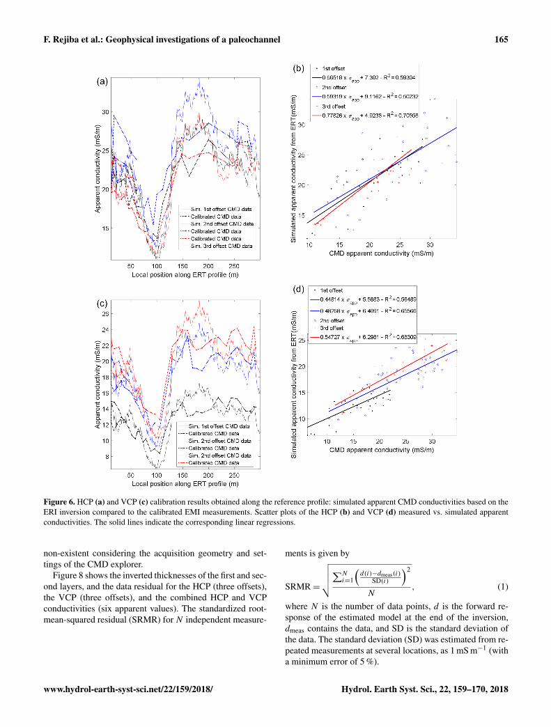
In order to compute the ECa of a layered ground, basedon measurements made using a horizontal or vertical mag-netic dipole configuration, we used the well-known electro-magnetic analytical solution for cylindrical model symme-try (given by Wannamaker et al. 1984; Ward and Hohmann,1988; Xiong, 1989). However, in the case of thin layers orhigh-frequency content, convergence problems can be en-countered in the numerical integration of the correspondingoscillating Bessel functions. At frequencies below 100 kHz,as in the case of the present study, the numerical filters de-veloped by Guptarsarma and Singh (1997) were found toprovide an efficient solution to this problem. The inversionscheme developed by Schamper et al. (2012) was used to in-vert the EMI measurements. For each offset and dipole ori-entation, a linear relationship (shifting and scaling) is deter-mined between each measured ECa and the ECa estimatedfrom the resistivity models (derived from the ERI panel,Fig. 6). Once the calibration has been done, the new EMIinversion matches the ERI used for the calibration, whichillustrates the validity of the procedure. Despite the linearrelationship assessed between the EMI and ERI resistivi-ties, several non-linear operations are applied: (1) ERI lo-cal 1-D models along the profile are used to simulate EMImeasurements, (2) EMI field data are then fitted (linearly)to those simulations using a non-linear optimization proce-dure to estimate calibration factors, and (3) finally the cal-ibrated/shifted data are inverted with a non-linear forwardmodelling. Each of the previous operations implies a neces-
sary check to ensure that the calibration process has been cor-rectly applied. Step (3) does not guarantee that estimated in-terfaces will match the ERT interfaces (1) if the fixed/chosenresistivities are not correct, or (2) if EMI does not integratethe ground in the same way as the ERI in the case of stronganisotropy. This does not seem to be the case here, since agood match is obtained.
The correlation coefficients range between 0.5 and 0.7.Such values can be explained by several sources of errorsin the estimation of the EMI apparent conductivities alongthe reference profile: (1) the differences in the location be-tween the EMI measurements used for the calibration andthe ERI profile, (2) the fact that the 1-D model used for theEMI modelling is extracted from the inversed 2-D resistivitysection, and (3) the difference of sensitivity between the ERIand EMI data. The regressions indicate the need of a strongercorrection for the VCP configuration than for the HCP con-figuration. The scaling correction decreases as a function ofoffset, particularly for the HCP, which can be explained bythe fact that small offsets are more sensitive to positioningand orientation errors, as well as to natural near-surface vari-abilities.
3.3 EMI inversion parameters
Once the calibration process is completed, the corrected, ap-parent HCP and VCP conductivities are inverted, followingtheir interpolation (by kriging) onto the same regular grid.The ERI results indicate a two-layer model (but do not high-light the topsoil), while the auger soundings show a topsoillayer of a few decimetres thickness above the conductive for-mation. Consequently, a three-layer model seems reasonablyjustified all over the site during the inversion process to repre-sent the studied area: a resistive topsoil, a conductive clayeyfilling, and a resistive sand/gravel layer. The resistivity ofeach layer corresponds to the peak values of the bimodal his-tograms of the reference 1 m spaced ERI profile, as shownin Fig. 7. The topsoil EC derived from the half-metre-spacedERI profile in the western portion is found to be very similarto the EC of the resistive layer inferred from the 1 m spacedERI profile – thus, the first and third layer EC are consideredto be equal. This leads to the following model for the meanEC of the three layers: σ1 = 13 mS m−1; σ2 = 72 mS m−1;σ3 = 13 mS m−1. It should be noted that the CMD explorer isoperated at a single frequency (10 kHz). The sounding heightwas taken to be 1 m for all the field measurements.
It is worth noting that the three-layer model chosen insteadof a two-layer model, all over the site, might be questionable.Letting the inversion process decide between a three- or two-layer model could have been an option. In the present case,the difference between a two-layer or three-layer model isclearly negligible where the interpreted thickness of the top-soil (for the three-layer model) is less than a few decimetres.For such low thicknesses the topsoil can be considered as
F. Rejiba et al.: Geophysical investigations of a paleochannel 165
Figure 6. HCP (a) and VCP (c) calibration results obtained along the reference profile: simulated apparent CMD conductivities based on theERI inversion compared to the calibrated EMI measurements. Scatter plots of the HCP (b) and VCP (d) measured vs. simulated apparentconductivities. The solid lines indicate the corresponding linear regressions.
non-existent considering the acquisition geometry and set-tings of the CMD explorer.
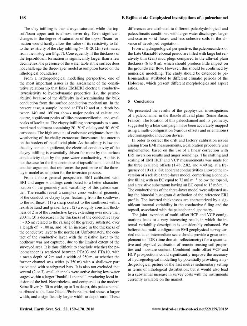
Figure 8 shows the inverted thicknesses of the first and sec-ond layers, and the data residual for the HCP (three offsets),the VCP (three offsets), and the combined HCP and VCPconductivities (six apparent values). The standardized root-mean-squared residual (SRMR) for N independent measure-
ments is given by
SRMR=
√√√√∑Ni=1
(d(i)−dmeas(i)
SD(i)
)2
N, (1)
where N is the number of data points, d is the forward re-sponse of the estimated model at the end of the inversion,dmeas contains the data, and SD is the standard deviation ofthe data. The standard deviation (SD) was estimated from re-peated measurements at several locations, as 1 mS m−1 (witha minimum error of 5 %).
166 F. Rejiba et al.: Geophysical investigations of a paleochannel
Figure 7. Histogram of the electrical resistivity values determined for the ERI section shown in Fig. 5.
Figure 8. Results of the CMD inversion, including the data residual (left column), for a three-layer model (1: topsoil; 2: conductive filling;and 3: resistive substratum). The thicknesses 1 and 2 correspond to the topsoil and conductive filling, respectively. The prospection heightis 1 m. The conductivities are set to σ1 = 13 mS m−1, σ2 = 72 mS m−1 and σ3 = 13 mS m−1. A noise level of 1 mS m−1 on the apparentconductivities was assumed, with a minimum relative error of 5 %. The black dashed line indicates the ERI reference profile location.
F. Rejiba et al.: Geophysical investigations of a paleochannel 167
3.4 EMI results
3.4.1 General trend
The layer thickness inversion was performed using three dif-ferent datasets: (1) the HCP dataset, (2) the VCP dataset, and(3) the combined HCP and VCP dataset (Fig. 8).
Whatever the dataset used for the inversion, the thicknesscomputed for the topsoil formation (indicated by “Thick-ness 1” in Fig. 8) is globally very small (blue), whereas thatcomputed for the conductive infilling (indicated by “Thick-ness 2”) has a significantly higher value (red), and vice versa.Although it varies in thickness, the conductive layer forma-tion spans most of the survey area, whereas the resistive top-soil formation varies mainly in two distinct locations: (1) thesouthwestern limit of the surveyed area, where it reaches adepth of 2 m, and (2) the mid-northern portion of the sur-veyed area, where its thickness never exceeds 0.6 m. In ad-dition, very small scale topsoil formations are scattered overthe surveyed area. In all places where the estimated thick-ness of the first layer is less than 20 cm, the topsoil can beconsidered as inexistent and a two-layered model is enoughto explain EMI data. Nevertheless, all of the observed top-soil formations appear to be correlated with a local increasein data residual. The thickness of the conductive infilling ly-ing below the topsoil formation ranges between 0 m, in thesouthwestern portion of the studied zone, and its maximumvalue of almost 2 m at the centre of the map.
The VCP mode increases the measured thickness of theshallowest portions of the topsoil layer, whereas the HCPmode tends to negate this layer over most of the surveyedarea (central part), where it is not extremely thick. This ten-dency appears to be correlated with a slight increase in thethickness of the second conductive layer.
The inversion of all data, in the form of a single dataset,appears to lead to a mixture of the properties inherent to eachof the constituent datasets. This outcome is particularly no-ticeable in the case of the topsoil formation, where certainstructures retrieved by both datasets are emphasized with re-spect to structures that are present in only one or the other ofthese.
3.4.2 Internal variability
In addition to strong meander wavelength variations, eachdipole orientation reveals different level of heterogeneities inthe material present in the conductive infilling, as well as thetopsoil. Concerning the material close to the surface (< 2 m),this variability is clearly illustrated by the auger soundings,whereas the conductive unit identified by the ERI section isconsiderably more complex. In simple terms, the thickness ofthe conductive material tends to decrease, wherever the siltyand sandy material reaches the surface.
It should be noted that the inversions observed for eachdipole orientation are not systematically preserved in the in-
version produced by combining the data from both dipoleorientations. This result indicates that in the present context,each orientation is complementary, and contributes a specificset of information. This is particularly relevant in the north-ern portion of the studied area, where the thickness of thefirst resistive layer is more variable when it is measured withthe horizontal dipole configuration (VCP) than with the HCPconfiguration.
The data residual has numerous peaks in the southwesternportion of the study zone. In this zone, the resistive topsoilreaches a thickness of 1 m, leading to EMI measurementswith a lower sensitivity (and thus lower signal-to-noise ra-tio, SNR). The combined HCP and VCP data inversion nat-urally leads to the occurrence of higher values of data resid-ual than in the case of the individual HCP or VCP inver-sions. Indeed, it is difficult to compare the data residual mapsbetween the three proposed datasets (i.e. HCP alone, VCPalone, and both) as the physical contribution associated witheach dataset inversion result is related to the coupled dataset–model used for the inversion. HCP and VCP modes do notintegrate the ground in the same way exactly. If the groundwithin the footprint of the EMI system is a bit far from atabular model, then the interpretation with local 1-D mod-els can be more difficult with both datasets combined thanwith only one of the two sets analysed. The difficulty to in-vert the HCP and VCP datasets jointly also arises because(1) the locations of the soundings between the two surveysare not exactly the same as the modes cannot be acquired atthe same time, (2) the heights varies differently, and (3) thepitch and roll are not constant. For those last two points onecould imagine the monitoring of these “flight” parameters tocorrect the data, which is routinely done for airborne elec-tromagnetic surveys. But this feature does not exist at thepresent time for ground-based EMI devices.
4 Discussion
In the present study, the outcomes of ERI and EMI surveysintegrate quite satisfactorily the lithological information pro-vided by the auger soundings, but have not yet been checkedwith exhaustive hydrological information. During the pre-sented geophysical campaign (low-water period), the wa-ter level measured from PTA02 to PTA04 and from PTA11to PTA13 locations indicate a groundwater situated at 1 mdepth, roughly at the interface between the clay infilling andthe upper geological unit (Fig. 4). In the survey area the wa-ter table could rise close to the surface at high-water peri-ods, which implies that the conductivity of the topsoil/loamformation should increase. In the closest piezometer located1 km west from the prospected site, the water table was sit-uated at 70 cm below the surface. The EC measured in thesame piezometer in 2011 was 640 µS cm−1 (15.6�m) andshowed a seasonal variation of the water table of approxi-mately 60 cm (Voies Naviguables de France (VNF) Techni-cal Report, 2011).
168 F. Rejiba et al.: Geophysical investigations of a paleochannel
The clay infilling is thus always saturated while the top-soil/loam upper unit is almost never dry. Even significantchanges in the degree of saturation of the topsoil/loam for-mation would hardly allow the value of its resistivity to fallto the resistivity of the clay infilling (∼ 10–20�m) estimatedfrom the histogram (Fig. 7). Consequently, if the thickness ofthe topsoil/loam formation is significantly larger than a fewdecimetres, the presence of the water table at the surface doesnot challenge the three-layer model assumption based on thelithological boundaries.
From a hydrogeological modelling perspective, one ofthe most important issues is the assessment of the consti-tutive relationship that links EMI/ERI electrical conductiv-ity/resistivity to hydrodynamic properties (i.e. the perme-ability) because of the difficulty in discriminating the bulkconduction from the surface conduction mechanism. In thepresent case, a sample located at PTA12 and at a depth be-tween 140 and 160 cm shows major peaks of calcite andquartz, significant peaks of illite-montmorillonite, and smallpeaks of kaolinite. The clayey infilling corresponds to a satu-rated marl sediment containing 20–30 % of clay and 50–60 %carbonate. The high amount of carbonate originates from theweathering of the chalky cretaceous limestones that outcropon the borders of the alluvial plain. As the salinity is low andthe clay content significant, the electrical conductivity of theclayey infilling is essentially driven far more by the surfaceconductivity than by the pore water conductivity. As this isnot the case for the first decimetre of topsoil/loam, it could beanother argument that reinforces the pertinence of the three-layer model assumption for the inversion process.
From a more general perspective, EMI calibrated withERI and auger soundings contributed to a better character-ization of the geometry and variability of this paleomean-der. The results reveal a complex cross-sectional geometryof the conductive clayey layer, featuring from the southwestto the northeast: (1) a sharp contact to the southwest with aresistive sand and gravel layer, (2) a roughly constant thick-ness of 2 m of the conductive layer, extending over more than200 m, (3) a decrease in the thickness of the conductive layer(∼ 0.5 m) related to the raising of the gravely substrate, overa length of ∼ 100 m, and (4) an increase in the thickness ofthe conductive layer to the northeast. Unfortunately, the con-tact of the conductive layer with the resistive layer to thenortheast was not captured, due to the limited extent of thesurveyed area. It is thus difficult to conclude whether the pa-leomeander is restricted between PTA03 and PTA10, witha mean depth of 2 m and a width of 250 m, or whether theformer channel was wider (> 350 m) with a shallower partassociated with sand/gravel bars. It is also not excluded thatseveral (2 or 3) small channels were active during low-waterstages within a larger “bankfull channel”, producing local in-cision of the bed. Nevertheless, and compared to the modernSeine River (∼ 50 m wide, up to 5 m deep), this paleochannelattributed to the Late Glacial/Preboreal period shows a largerwidth, and a significantly larger width-to-depth ratio. These
differences are attributed to different paleohydrological andpaleoclimatic conditions, with larger water discharges, largerand coarser solid fluxes, and less cohesive soils in the ab-sence of developed vegetation.
From a hydrogeological perspective, the paleomeanders ofthe Late Glacial/Preboreal period are filled with large but rel-atively thin (2 m) mud plugs compared to the alluvial plainthickness (6 to 8 m), which should produce little impact onthe groundwater flow. However, this should be confirmed bynumerical modelling. The study should be extended to pa-leomeanders attributed to different climatic periods of theHolocene, which present different morphologies and aspectratios.
5 Conclusion
We presented the results of the geophysical investigationsof a paleochannel in the Bassée alluvial plain (Seine Basin,France). The location of this paleochannel and its geometry,suggested by a lidar campaign, have been accurately mappedusing a multi-configuration (various offsets and orientations)electromagnetic induction device.
In order to correct the drift and factory calibration issuesarising from EMI measurements, a calibration procedure wasimplemented, based on the use of a linear correction withERI inversion results and auger soundings. The shifting andscaling of EMI HCP and VCP measurements was made forthe three available offsets (1.48, 2.82, and 4.49 m), at a fre-quency of 10 kHz. Six apparent conductivities allowed the in-version of a reliable three-layer model, comprising a conduc-tive filling with an EC equal to 72 mS m−1 below the topsoil,and a resistive substratum having an EC equal to 13 mS m−1.The conductivities of the three-layer model were adjusted us-ing the bimodal histogram distribution of the reference ERIprofile. The inverted thicknesses are characterized by a sig-nificant internal variability in the conductive filling and thetopsoil, associated with the paleochannel geometry.
The joint inversion of multi-offset HCP and VCP config-urations leads to a very interesting result, in which the in-ternal variability description is considerably enhanced. Webelieve that multi-configuration EMI geophysical survey car-ried out at an intermediate scale should provide a great com-plement to TDR (time domain reflectometry) for a quantita-tive and physical calibration of remote sensing soil proper-ties and moisture content. Combined multi-offset VCP andHCP prospections could significantly improve the accuracyof hydrogeological modelling by potentially providing a hy-drogeological picture of the first metres sedimentary settingin terms of lithological distribution; but it would also leadto a substantial increase in survey costs with the instrumentscurrently available on the market.
F. Rejiba et al.: Geophysical investigations of a paleochannel 169
Data availability. In order to access the data, we ask researchers tocontact the corresponding author ([email protected]).
Competing interests. The authors declare that they have no conflictof interest.
Acknowledgements. This research was supported by the PIRENSeine research programme (2015–2019). We extend our warmthanks to Christelle Sanchez for her participation in the geophysicalsurvey and to Laurence LeCallonnec for carrying out the XRDexperiment.
Edited by: Mauro GiudiciReviewed by: Bradley Weymer and two anonymous referees
References
Antoine, P., Coutard, J.-P., Gibbard, P., Hallegouet, B., Lautridou,J.-P., and Ozouf, J.-C.: The Pleistocene rivers of the EnglishChannel region, J. Quaternary Sci., 18, 227–243, 2003.
Benech, C., Lombard, P., Rejiba, F., and Tabbagh, A: Demonstrat-ing the contribution of dielectric permittivity to the in-phaseEMI response of soils: example of an archaeological site inBahrain, Near Surf. Geophys., 14, 337–344, 2016.
Berger, G., Delpont, G., Dutartre, P., and Desprats, J.-F.: Evolutionde l’environnement paysager de la vallée de la Seine – Cartogra-phie historique et prospectives des explorations alluvionnaires dela Bassée, French Geological Survey (BRGM) report R 38 726,39 pp., 1995.
Caillol, M., Camart, R., and Frey, C.: Synthèse bibliographique surla géologie, l’hyrogéologie et les ressources en matériaux de larégion de Nogent-sur-Seine (Aube), French Geological Survey(BRGM) report 77 SGN 303 BDP, 108 pp., 1977.
Dahlin, T. and Zhou, B.: A numerical comparison of 2-D resistivityimaging with 10 electrode arrays, Geophys. Prospect., 52, 379–398, 2004.
Dahlin, T. and Zhou, B.:Multiple-gradient array measurements formultichannel 2-D resistivity imaging, Near Surf. Geophys., 4,113–123, 2006.
Delefortrie, S., De Smedt, P., Saey, T., Van De Vijver, E., and VanMeirvenne, M.: An efficient calibration procedure for correctionof drift in EMI survey data, J. Appl. Geophys., 110, 115–125,2014.
Deleplancque, B. : Caractérisation des hétérogénéités sédimen-taires d’une plaine alluviale: Exemple de l’évolution de la Seinesupérieure depuis le dernier maximum glaciaire, PhD Thesis,PSL Research University, Paris, France, 273 pp., 2016.
De Smedt, P., Van Meirvenne, M., Meerschman, E., Saey, T., Bats,M., Court-Picon, M., De Reu, J., Zwertvaegher, A., Antrop, M.,Bourgeois, J., and De Maeyer, P.: Reconstructing palaeochannelmorphology with a mobile multicoil electromagnetic inductionsensor, Geomorphology, 130, 136–141, 2011.
Everett, M. E.: Theoretical developments in electromagnetic in-duction geophysics with selected applications in the near sur-face, Surv. Geophys., 33, 29–63, 2012.
Fitterman, D. V., Menges, C. M., Al Kamali, A. M., and Jama, F.E.: Electromagnetic mapping of buried paleochannels in easternAbu Dhabi Emirate, UAE, Geoexploration, 27, 111–133, 1991.
Friedman, S. P.: Soil properties influencing apparent electrical con-ductivity: a review, Comput. Electron. Agr., 46, 45–70, 2005.
Furman, A., Ferré, T., and Warrick, A. W.: A sensitivity analysisof electrical resistivity tomography array types using analyticalelement modeling, Vadose Zone J., 2, 416–423, 2003.
Guptasarma, D. and Singh, B.: New digital linear filters for HankelJ0 and J1 transforms, Geophys. Prospect., 45, 745–762, 1997.
Jordan, D. W. and Prior, W. A.: Hierarchical Levels of Heterogene-ity in a Mississippi River Meander Belt and Application to Reser-voir Systems: Geologic Note, AAPG Bulletin, 76, 1601–1624,1992.
Huang, H.: Depth of investigation for small broadband electromag-netic sensors, Geophysics, 70, G135–G142, 2005.
Lavoué, F., Van Der Kruk, J., Rings, J., André, F., Moghadas, D.,Huisman, J. A., Lambot, S, Weihermüller, L., Vanderborght, J.,and Vereecken, H.: Electromagnetic induction calibration usingapparent electrical conductivity modelling based on electrical re-sistivity tomography, Near Surf. Geophys., 8, 553–561, 2010.
Loke, M. H., Acworth, I., and Dahlin, T.: A comparison of smoothand blocky inversion methods in 2-D electrical imaging surveys,Explor. Geophys., 34, 182–187, 2003.
Mégnien, F. : Possibilités aquifères des alluvions du val de Seine en-tre Nogent-sur-Seine et Montereau, incluant la carte géologiqueet géomorphologique de la Bassée, French Geological Survey(BRGM) report 65-DSGR-A-076, 452 pp., 1965.
Miall, A. D.: Reservoir Heterogeneities in Fluvial Sandstones:Lessons from Outcrop Studies, AAPG Bulletin, 72, 682–697,1988.
Mordant, D. : La Bassée avant l’histoire : archéologie et gravièresen Petite-Seine, Association pour la promotion de la recherchearchéologique en Ile-de-France, Nemours, 143 pp., 1992.
Nabighian, M. N.: Electromagnetic methods in applied geo-physics (Vol. 1), SEG Books, 1988a.
Nabighian, M. N.: Electromagnetic methods in applied geo-physics (Vol. 2), SEG Books, 1988b.
Pastre, J.-F., Limondin-Lozouet, N., Leroyer, C., Ponel, P., andFontugne, M.: River system evolution and environmentalchanges during the Lateglacial in the Paris Basin (France), Qua-ternary Sci. Rev., 22, 2177–2188, 2003.
Rhoades, J. D., Raats, P. A. C., and Prather, R. J.: Effects of liquid-phase electrical conductivity, water content, and surface conduc-tivity on bulk soil electrical conductivity, Soil Sci. Soc. Am.J., 40, 651–655, 1976.
Schamper, C., Rejiba, F., and Guérin, R.: 1-D single-site and lat-erally constrained inversion of multifrequency and multicompo-nent ground-based electromagnetic induction data – Applicationto the investigation of a near-surface clayey overburden, Geo-physics, 77, WB19–WB35, 2012.
Simon, F. X., Sarris, A., Thiesson, J., and Tabbagh, A.: Mappingof quadrature magnetic susceptibility/magnetic viscosity of soils
170 F. Rejiba et al.: Geophysical investigations of a paleochannel
by using multi-frequency EMI, J. Appl. Geophys., 120, 36–47,2015.
Spies, B. R.: Depth of investigation in electromagnetic soundingmethods, Geophysics, 54, 872–888, 1989.
Tabbagh, A.: Applications and advantages of the Slingramelectromagnetic method for archaeological prospecting, Geo-physics, 51, 576–584, 1986.
Thiesson, J., Kessouri, P., Schamper, C., and Tabbagh, A.: Aboutcalibration of frequency domain electromagnetic devices used innear surface surveying, Near Surf. Geophys., 12, 481–491, 2014.
VNF (Voies navigables de France): Etat des lieux de la piézométriede la petite Seine, Technical Report, 58 pp., 2011 (in french).
Wannamaker, P. E., Hohmann, G. W., and Sanfilipo, W. A.:Electromagnetic modeling of three-dimensional bodies in lay-ered earths using integral equations, Geophysics, 49, 60–74,https://doi.org/10.1190/1.1441562, 1984.
Ward, S. H. and Hohmann, G. W.: Electromagnetic theory for geo-physical applications, in: Electromagnetic methods in appliedgeophysics, Vol. 1: Theory, edited by: Nabighian, M. N., 131–311, 1988.
Xiong, Z.: Electromagnetic fields of electric dipoles embeddedin a stratified anisotropic earth, Geophysics, 54, 1643–1646,https://doi.org/10.1190/1.1442633, 1989.