Multidimensional Inequality Measurement: A Proposal 1 Christian List Nuffield College Oxford OX1 1NF, U.K. NUFFIELD COLLEGE WORKING PAPER IN ECONOMICS 19 NOVEMBER 1999 Abstract. Two essential intuitions about the concept of multidimensional inequality have been highlighted in the emerging body of literature on this subject: first, multidimensional inequality should be a function of the uniform inequality of a multivariate distribution of goods or attributes across people (Kolm, 1977); and, second, it should also be a function of the cross-correlation between distributions of goods or attributes in different dimensions (Atkinson and Bourguignon, 1982; Walzer, 1983). While the first intuition has played a major role in the design of fully-fledged multidimensional inequality indices, the second one has only recently received attention (Tsui, 1999); and, so far, multidimensional generalized entropy measures are the only inequality measures known to respect both intuitions. The present paper proposes a general method of designing a wider range of multidimensional inequality indices that also respect both intuitions, and illustrates this method by defining two classes of such indices: a generalization of the Gini coefficient, and a generalization of Atkinson's one- dimensional measure of inequality. JEL Classification: D31, D63, I31 Keywords: multidimensional inequality, multivariate majorization 1 The author wishes to express his gratitude to A. B. Atkinson, Christopher Bliss and David Miller for discussion, comments and suggestions.
NUFFIELD COLLEGE WORKING PAPER IN ECONOMICS19 NOVEMBER 1999
Abstract. Two essential intuitions about the concept of multidimensional inequality havebeen highlighted in the emerging body of literature on this subject: first,multidimensional inequality should be a function of the uniform inequality of amultivariate distribution of goods or attributes across people (Kolm, 1977); and, second,it should also be a function of the cross-correlation between distributions of goods orattributes in different dimensions (Atkinson and Bourguignon, 1982; Walzer, 1983).While the first intuition has played a major role in the design of fully-fledgedmultidimensional inequality indices, the second one has only recently received attention(Tsui, 1999); and, so far, multidimensional generalized entropy measures are the onlyinequality measures known to respect both intuitions. The present paper proposes ageneral method of designing a wider range of multidimensional inequality indices thatalso respect both intuitions, and illustrates this method by defining two classes of suchindices: a generalization of the Gini coefficient, and a generalization of Atkinson's one-dimensional measure of inequality.
1The author wishes to express his gratitude to A. B. Atkinson, Christopher Bliss and
David Miller for discussion, comments and suggestions.
- 1 -
1. Introduction
The concern of the present paper is the problem of multidimensional inequalitymeasurement. Suppose we are asked to evaluate the overall level of inequality insociety not just on the basis of one good/attribute -- or a one-dimensional item ofinformation -- for each person or household (e.g. each person's or household'sincome), but on the basis of several goods/attributes -- or a multidimensional vector ofinformation -- for each person or household (e.g. a vector whose different componentsrepresent a person's or households's income, level of education, level of access tohealth care etc.). Given different multidimensional distributions (each of whichassigns to each person or household in society a corresponding vector ofgoods/attributes), the problem of multidimensional inequality measurement is, inessence, to specify what it means to say that one such distribution is more unequalthan another and, as far as possible, to rank different distributions in an order ofinequality.
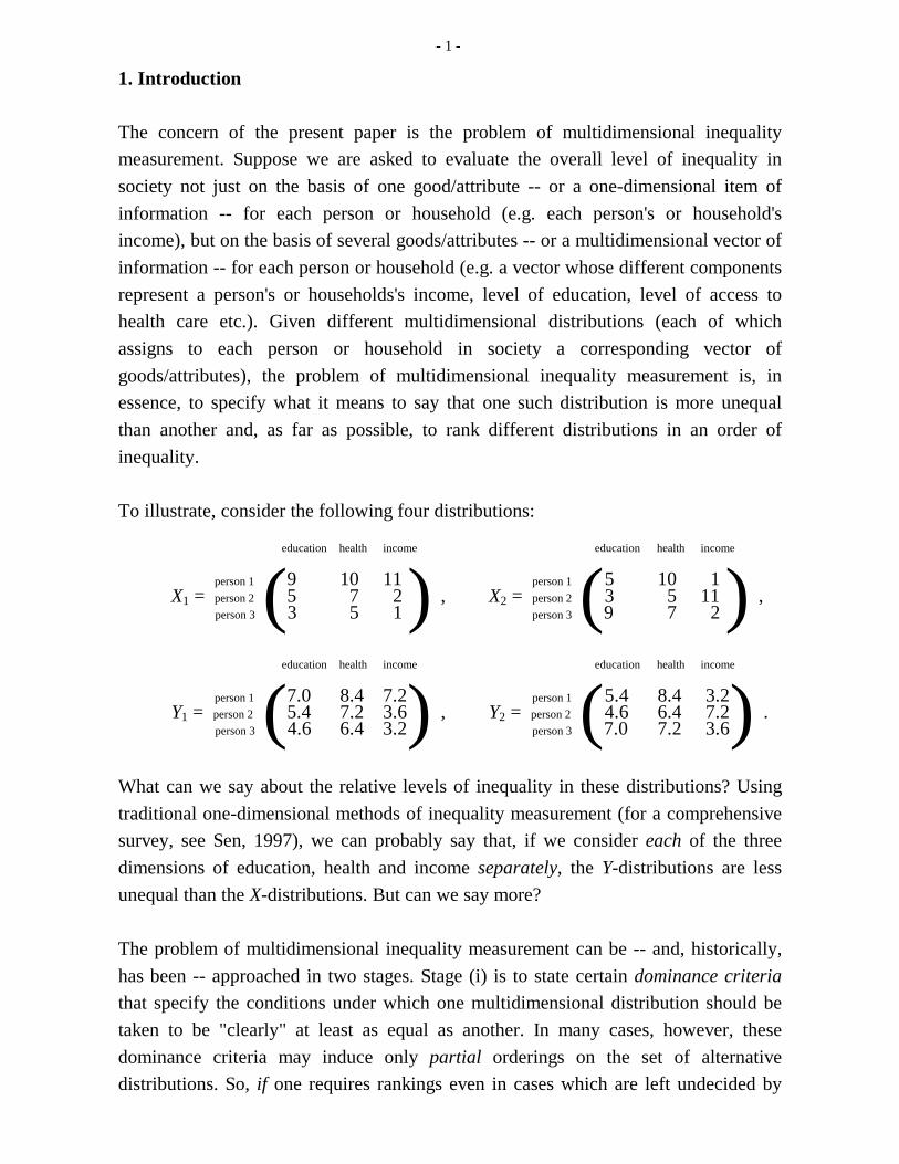
To illustrate, consider the following four distributions:
education health income education health income
person 1 9 10 11 person 1 5 10 1X1 = person 2 5 7 2 , X2 = person 2 3 5 11 , person 3 (3 5 1 ) person 3 (9 7 2 )
education health income education health income
person 1 7.0 8.4 7.2 person 1 5.4 8.4 3.2Y1 = person 2 5.4 7.2 3.6 , Y2 = person 2 4.6 6.4 7.2 . person 3 (4.6 6.4 3.2) person 3 (7.0 7.2 3.6)
What can we say about the relative levels of inequality in these distributions? Usingtraditional one-dimensional methods of inequality measurement (for a comprehensivesurvey, see Sen, 1997), we can probably say that, if we consider each of the threedimensions of education, health and income separately, the Y-distributions are lessunequal than the X-distributions. But can we say more?
The problem of multidimensional inequality measurement can be -- and, historically,has been -- approached in two stages. Stage (i) is to state certain dominance criteriathat specify the conditions under which one multidimensional distribution should betaken to be "clearly" at least as equal as another. In many cases, however, thesedominance criteria may induce only partial orderings on the set of alternativedistributions. So, if one requires rankings even in cases which are left undecided by
- 2 -
the specified dominance criteria, stage (ii) is to define an inequality index, consistentwith these dominance criteria, that maps each multidimensional distribution to a realnumber and thereby induces a complete ordering on the set of alternative distributions.
The study of multidimensional inequality was pioneered by Fisher (1956), whodeveloped the idea of a multidimensional distribution matrix, and, more recently, bythe seminal contributions of Kolm (1977), Atkinson and Bourguignon (1982) andWalzer (1983). Amongst Kolm's proposals with regard to stage (i) are the criteria thathave become known as uniform majorization (in essence, a multidimensionalgeneralization of the well-known Pigou-Dalton criterion) and directional/pricemajorization (a criterion that involves multiplying multidimensional distributions byprice vectors and comparing the resulting one-dimensional distributions). Thesecriteria are primarily sensitive to the uniform inequality of a multidimensionaldistribution across people. Kolm's criteria capture the idea that distribution Y1 is lessunequal than distribution X1, and that distribution Y2 is less unequal than distributionX2. Atkinson and Bourguignon have drawn our attention to the intuition thatmultidimensional inequality also depends on how systematic the correlation betweendistributions of different goods/attributes (and especially between inequalities indifferent dimensions) is and have developed appropriate dominance criteria. Sinceinequalities in different dimensions are more systematically cross-correlated indistributions X1 and Y1 than in distributions X2 and Y2, respectively, distribution X2
should thus be considered less unequal than distribution X1, and distribution Y2 shouldbe considered less unequal than distribution Y1. In a similar spirit, the political theoristWalzer developed the conception of complex equality, according to which overallequality consists not so much in local equality within each dimension (distributivesphere in Walzer's terminology), but in the extent to which local inequalities indifferent dimensions cancel each other out, by advantaging and disadvantagingdifferent people in different dimensions. So complex equality would be better realizedin distributions X2 and Y2 than in distributions X1 and Y1, respectively. Note thatseparate one-dimensional inequality evaluation in each dimension is insufficient totake account of problems of cross-correlation: distributions X1 and X2 have identicallocal levels of inequality in each of the three separate dimensions, and so dodistributions Y1 and Y2.
Although these pioneers primarily addressed stage (i), their work inspired subsequentproposals as to how one could approach stage (ii) and construct fully-fledgedmultidimensional inequality indices (e.g. Maasoumi, 1986; Tsui, 1995, 1999;Koshevoy and Mosler, 1997). While all these proposed inequality measures make use
- 3 -
of the dominance criteria proposed by Kolm, the Atkinson-Bourguignon-Walzerintuition that a multidimensional inequality measure should also be sensitive to thecross-correlation between inequalities in different dimensions has only recentlyreceived explicit attention in the design of such measures2. Tsui (1999) formallyintroduced a correlation-sensitive majorization criterion into the debate and showedthat this new criterion, together with Kolm's uniform majorization criterion and astandard set of axioms, leads to the class of multidimensional generalized entropymeasures. However, Tsui's result uses a version of the somewhat controversial axiomof (additive) decomposability, which, by requiring us to ignore some -- arguablyuseful -- information in a distribution, is known to rule out all but entropy-basedmeasures in various economic and information-theoretic contexts (see Sen, 1997,chapter A.5, for a discussion of this axiom).
It is therefore worth asking whether it is possible to design other multidimensionalinequality measures that satisfy both Kolm's criteria and the correlation-sensitive majorization criterion introduced by Tsui, thereby respecting the intuition that (a)uniform inequalities across people and (b) cross-correlations between inequalities indifferent dimensions matter (i.e. the intuition that (a) Y1 is more equal than X1, and Y2
is more equal than X2, and (b) X2 is more equal than X1, and Y2 is more equal than Y1).
The present paper seeks to answer this question. Its purpose is methodological andsubstantive. On the methodological side, the paper presents a rather general way ofdefining multidimensional inequality indices by first transforming multidimensionaldistributions into suitable 'welfare-concentration curves' (a term from Kolm, 1977)and then constructing a multidimensional inequality index on the basis of a suitableone-dimensional aggregation function that takes these 'welfare-concentration curves'as its input and that respects the generalized Lorenz-ordering of these curves. On thesubstantive side, this method is then used to construct two examples ofmultidimensional inequality indices, and it is shown that these indices satisfy all of theabove mentioned desiderata. One example is a generalization of the Gini coefficient,the other is a generalization of Atkinson's one-dimensional measure of inequality(Atkinson, 1970). It is also shown that an extension of Kolm's less frequently invoked
2In terms of the conditions stated below, it can easily be verified that condition (CIM)
is violated by the inequality indices proposed in Tsui's 1995 paper subtitled, somewhatmisleadingly in view of Atkinson & Bourguignon (1982), "The Atkinson-Kolm-SenApproach": Tsui's relative inequality index (1995, theorem 1.), for instance, can assign alower value to X1 than to X2 and a lower value to Y1 than to Y2, contrary to the Atkinson-Bourguignon-Walzer intuition that systematic cross-correlations between inequalities indifferent dimensions increase overall inequality.
- 4 -
criterion, directional/price majorization, namely non-negative directional/pricemajorization, already captures the Atkinson-Bourguignon-Walzer intuition aboutcross-correlation: we shall prove that the correlation-sensitive majorization criterionintroduced by Tsui (1999) is in fact a (proper) sub-criterion of non-negativedirectional/price majorization.
After some basic definitions (section 2.), it will be requisite to survey variousdominance criteria and explore their logical interrelations (section 3.); we shall thenexplain the present use of 'welfare-concentration curves' (section 4.), and we shallfinally turn to the construction of fully-fledged inequality indices (section 5.).
2. Definitions and Basic Axioms
Let N = {1, 2, ..., n} be a set of persons or households (for simplicity, hereafter'persons'), and K = {1, 2, ..., k} a set of goods/attributes, dimensions or distributivespheres.
A multidimensional distribution is an n×k matrix X = (xij) over the non-negative realnumbers such that the sum of each column is non-zero, where xij represents person i'sshare of good/attribute j. Let M (n,k) be the set of all such matrices. The row vectorsx1, x2, ..., xn represent different persons' vectors of goods/attributes. The distributionsX1, X2, Y1 and Y2 above are examples of multidimensional distributions for n=3 andk=3.
A multidimensional inequality index is a function In : M (n,k) → R, where In(X) ≥ In(Y)is interpreted to mean "the overall level of multidimensional inequality in distributionX is at least as great as that in distribution Y".
The following basic axioms are straightforward generalizations of their familiar one-dimensional counterparts (see Tsui, 1999):
CONTINUITY (C). In is a continuous function.
ANONYMITY (A). For any n×n permutation matrix Π permuting the rows of X, In(X) =In(ΠX).
- 5 -
NORMALIZATION (N). If all rows of a distribution X are identical (i.e. the distributionin each dimension is perfectly equal), In(X) = 0.
REPLICATION INVARIANCE (RI). Given a n×k distribution matrix X, let Y be then*r×k distribution matrix defined by
XY = X (with r 'replications' of X).
(⋅⋅⋅) X
Then In*r(Y) = In(X).
RATIO-SCALE INVARIANCE (RS). For any n×n diagonal matrix Λ=diag(λ1, λ2, ..., λn)(with each λi>0), In(ΛX) = In(X).
These axioms by themselves, however, are insufficient to guarantee that amultidimensional inequality index is in any substantive sense 'egalitarian', i.e. that itrespects the various intuitions about multidimensional inequality briefly introduced inthe introduction. For this reason, our present list of axioms needs to be supplementedwith the dominance criteria capturing these intuitions.
3. Dominance Criteria
In the present section, we will survey some of the most important dominance criteriaproposed in the literature and explain how they are logically interrelated. In thiscontext, we will prove a new result showing that the correlation-sensitive criterionintroduced by Tsui (1999) is a subcriterion of non-negative directional majorization.
Each of the dominance criteria to be stated represents a proposed answer to thequestion of when a distribution X is "clearly" at least as equal as, and can therefore besaid to (at least weakly) dominate, a distribution Y.
The first two dominance criteria to be stated have been suggested by Kolm (1977) andare essentially generalizations of the one-dimensional Pigou-Dalton criterion,according to which any transfer from a poorer person to a richer person increasesinequality, other things remaining equal. Accordingly, if a distribution X can beobtained from a distribution Y by uniformly redistributing attributes so as to reducethe 'inequality-gap' between two or more persons, then X dominates Y. Define aPigou-Dalton matrix to be an n×n matrix P = λ*E + (1-λ)*Q, where E is the n×n
- 6 -
identity matrix and Q is a permutation matrix which transforms other matrices byinterchanging two rows.
UNIFORM PIGOU-DALTON MAJORIZATION (UPD). (X,Y)∈UPD and XºUPDY("distribution X dominates distribution Y according to (UPD)") if and only if X = TYwhere T is a finite product of Pigou-Dalton matrices. XÂUPDY ("distribution X strictlydominates distribution Y according to (UPD)") if, in addition, X cannot be derivedfrom Y by permuting the rows of Y.
Define a bistochastic matrix to be an n×n matrix B = (bij) such that, for all j, ∑ ibij=1,and for all i, ∑ jbij=1.
UNIFORM MAJORIZATION (UM). (X,Y) ∈UM and XºUMY if and only if X = BY,where B is a bistochastic matrix. XÂUMY if, in addition, X cannot be derived from Yby permuting the rows of Y.
It is easily verified that, for the examples of multidimensional distributions given inthe introduction, Y1ÂUMX1 and Y2ÂUMX2.
To introduce Kolm's criterion of directional/price majorization (1977), we first needto introduce the one-dimensional concept of generalized Lorenz-dominance, in shortGL-dominance.
We shall say that the vector (s1, s2, ..., sn) ∈ Rn GL-dominates3 the vector (t1, t2, ...,tn) ∈ Rn if, for all j,
∑ i∈{1, 2, ..., j}s'i ≥ ∑ i∈{1, 2, ..., j}t'i ,
3This is the concept of generalized Lorenz-dominance because, when we compare the
vectors (s1, s2, ..., sn) and (t1, t2, ..., tn) here, we do not consider their normalized Lorenzcurves as in the standard definition of Lorenz-dominance, i.e. we do not normalize (s1, s2, ...,sn) and (t1, t2, ..., tn) by multiplying them by the inverses of the means of the si and of the ti,respectively. For a discussion of generalized Lorenz dominance, see Shorrocks (1983) andSen (1997, appendix A.3).
- 7 -
where (s'1, s'2, ..., s'n) and (t'1, t'2, ..., t'n) are permutations of (s1, s2, ..., sn) and (t1, t2, ...,tn), respectively, such that s'1≤s'2≤...≤s'n and t'1≤t'2≤...≤t'n. The relation of GL-dominance is said to be strict if at least one of the above inequalities is strict.
Intuitively, the generalized Lorenz curve of an (income) vector (s1, s2, ..., sn) can beobtained by, firstly, rewriting the vector (s1, s2, ..., sn) as (s'1, s'2, ..., s'n) such that theincomes of the n persons are arranged in an increasing order s'1≤s'2≤...≤s'n; secondly,by plotting the proportion of persons j/n, ranging from 0 = 0/n to 1 = n/n, on the x-axisagainst the total income ∑ i∈{1, 2, ..., j}s'i controlled by the poorest j/n of society (thepoorest j persons) on the y-axis and connecting these points with line-segments. Then(s1, s2, ..., sn) GL-dominates (t1, t2, ..., tn) if the generalized Lorenz curve of (s1, s2, ...,sn) lies nowhere below that of (t1, t2, ..., tn), and the dominance is strict if the twocurves do not coincide.
DIRECTIONAL/PRICE MAJORIZATION (DM). (X,Y) ∈DM and XºDMY if and only if,for all price vectors a∈Rk, the vector Xa GL-dominates the vector Ya. XÂDMY if, inaddition, X cannot be derived from Y by permuting the rows of Y.
The logical connection between the previous dominance criteria and directional/pricemajorization is characterized by the following proposition:
We can extend the dominance relation of (DM) by restricting the set of relevant pricevectors to all non-negative ones.
NON-NEGATIVE DIRECTIONAL/PRICE MAJORIZATION (DM+). (X,Y) ∈DM+ andXºDM+Y if and only if, for all price vectors a∈R+
k, the vector Xa GL-dominates thevector Ya. XÂDM+Y if, in addition, X cannot be derived from Y by permuting the rowsof Y.
Obviously, DM⊆DM+. Below we shall in fact see that DM⊂ DM+.
Tsui (1999) introduced a dominance criterion that explicitly captures the Atkinson-Bourguignon-Walzer intuition about cross-correlation. If the only difference betweentwo multidimensional distributions X and Y is that there is a stronger positivecorrelation between advantaged positions within different dimensions and alsobetween disadvantaged positions within different dimensions under Y than under X
- 8 -
(i.e. under Y, someone who is well-off in one dimension is more likely to be well-offacross the board than under X; and, under Y, someone who is badly off in onedimension is more likely to be badly off across the board than under X), then Xdominates Y:
Define a correlation increasing transfer as follows (Boland & Proschan, 1988). Giventwo row vectors x = (x1, x2, ..., xk) and y = (y1, y2, ..., yk), let x ∧ y = (min(x1, y1),min(x2, y2), ..., (min(xk, yk)), and let x ∨ y = (max(x1, y1), max(x2, y2), ..., max(xk, yk)). Adistribution Y can be derived from a distribution X by a correlation increasing transferif, for some row indices i and j (i≠j), yi = xi ∧ xj and yj = xi ∨ xj, and, for all m∉ {i, j},xm = ym. Such a transfer is strict if Y≠X and Y is not just the result of swapping therows i and j in X. CORRELATION INCREASING MAJORIZATION (CIM). (X,Y) ∈CIM and XºCIMY if andonly if Y can be derived from X by a permutation of rows and a finite sequence ofcorrelation increasing transfers. XÂCIMY if, in addition, at least one of thesecorrelation increasing transfers is strict.
For the examples of multidimensional distributions given in the introduction, X1 andY1 can be derived, respectively, from X2 and Y2 by a sequence of strict correlationincreasing transfers, whence X2ÂCIMX1 and Y2ÂCIMY1.
The following proposition shows that (UM) (including its subrelation (UPD)) and(CIM) are logically independent.
Proposition 3.3. (Tsui, 1999) UM∩ CIM={(X,Y) : X can be derived from Y by apermutation of rows}, i.e. there exists no pair of distributions X and Y such thatXÂUMY and XÂCIMY.
We will now prove that (CIM) defines a subrelation of (DM+), but not of (DM), alogical connection that may not be at first sight obvious (whence DM≠DM+ and, sinceDM⊆DM+, DM⊂ DM+).
Proposition 3.4. CIM⊂ DM+.
Proof. Since UM⊄ CIM, but UM⊂ DM+, CIM≠DM+. It is thus sufficient to prove thatCIM⊆DM+. Suppose XºCIMY, i.e. there exists a finite sequence X = QX0, X1, ..., Xm =Y such that, for each i, Xi+1 can be derived from Xi by a correlation increasing transferand Q is a row-permutation matrix. We need to show that, for all price vectors a∈R+
k,
- 9 -
Xa GL-dominates Ya. Let a∈R+k. Since X can be obtained from X0 by a permutation of
rows, the generalized Lorenz curves of Xa and X0a are identical, and, trivially, Xa(weakly) GL-dominates X0a. We will now show that, for each i, Xia GL-dominatesXi+1a. Write Xi = (bij) and Xi+1 = (cij). Now there exist row-indices p and q (p≠q) suchthat, for each j, cpj = min(bpj, bqj) and cqj = max(bpj, bqj) and, for all r∉ {p, q} and all j,crj = brj. Then, for all r∉ {p, q}, the rth components of Xia and Xi+1a conincide andequal br1a1+br2a2+...+brkak. However,
pth component of Xi+1a = min(bp1,bq1)a1+min(bp2,bq2)a2+...+min(bpk,bqk)ak
≤ pth component of Xia = bp1a1+bp2a2+...+bpkak ,qth component of Xia = bq1a1+bq2a2+...+bqkak
≤ qth component of Xi+1a = max(bp1,bq1)a1+max(bp2,bq2)a2+...+max(bpk,bqk)ak.Hence the generalized Lorenz curve of Xi+1a lies nowhere above that of Xia, and XiaGL-dominates Xi+1a. But GL-dominance is transitive, and so X GL-dominates Y. Sincethis holds for any a∈R+
k, XºDM+Y. If, in addition, XÂCIMY, then X and Y cannot bepermutations of each other, and thus XÂDM+Y, too. Q.E.D.
Proposition 3.5. CIM⊄ DM. In fact, whenever Y can be obtained from X by a strictcorrelation-increasing transfer, (X,Y)∉ DM.
Proof. Suppose Y can be obtained from X by a strict correlation-increasing transfer.Then there exist row indices i and j (i≠j) such that yi = xi ∧ xj and yj = xi ∨ xj, and, forall m∉ {i, j}, xm = ym. Moreover, Y≠X and Y is not just the result of swapping the rows iand j in X. Then, for at least two column indices, p and q, it must be the case thatxip>xjp and xiq<xjq (if necessary swap the labels i and j). Assume, for a contradiction,(X,Y)∈DM. Then, for all a∈Rk, Xa GL-dominates Ya. Consider the price vector awhose pth and qth components equal (-ap) and aq, respectively, where ap, aq > 0 (e. g.ap=aq=1) and whose other entries are all 0. By assumption, Xa GL-dominates Ya (notethat Xa and Ya differ from each other only in rows i and j). This implies thateither
row i of Ya = yip(-ap) + yiqaq = xjp(-ap) + xiqaq
≤ row i of Xa = xip(-ap) + xiqaq ,row j of Xa = xjp(-ap) + xjqaq
≤ row j of Ya = yjp(-ap) + yjqaq = xip(-ap) + xjqaq
orrow j of Ya = yjp(-ap) + yjqaq = xip(-ap) + xjqaq
≤ row i of Xa = xip(-ap) + xiqaq ,row j of Xa = xjp(-ap) + xjqaq
≤ row i of Ya = yip(-ap) + yiqaq = xjp(-ap) + xiqaq
- 10 -
From the first set of inequalities, we get(i) xjp≥xip, xiq≤xjq ,
and, from the second set of inequalities, we get(ii) xjq≤xiq, xip≥xjp.
Now (i) contradicts xip>xjp, and (ii) contradicts xiq<xjq. Consequently, (X,Y)∉ DM.Q.E.D.
To summarize, the logical connections between the stated dominance criteria are asfollows:
In particular, (DM+) is the only one of the stated dominance criteria that is sensitiveboth to the uniform inequality of a multidimensional distribution across people and tothe cross-correlation between inequalities in different dimensions of goods/attributes.
4. Welfare Concentration Curves
We have already defined what it means to say that one vector in Rn GL-dominatesanother. Given a distribution matrix X, the basic idea of the present section is, first, touse a suitable function u : R+
k → R+ to aggregate each person's row-vector ofgoods/attributes into an overall evaluation figure for this person (representing howwell-off this person is in terms of his or her share of goods across the differentdimensions) and, second, to assess the resulting vector of evaluation figures byconsidering its generalized Lorenz curve, to be called the welfare concentration curveof the distribution X for the aggregation function u.
For any two distribution matrices X and Y and an aggregation function u, we can thenask whether the corresponding welfare concentration curve of X lies nowhere belowthat of Y, i.e. whether (u(x1), u(x2), ..., u(xn)) GL-dominates (u(y1), u(y2), ..., u(yn)).
The following three propositions give us some important information about whatproperties the aggregation function u : R+
k → R+ must satisfy in order for the relationof GL-dominance between corresponding welfare concentration curves to include UM(including UPD), CIM and DM+ (including DM).
- 11 -
Let X and Y be two multidimensional distribution matrices with row vectors x1, x2, ...,xn and y1, y2, ..., yn, respectively. Given a function u : R+
k → R+, we shall say that X(strictly) u-dominates Y if (u(x1), u(x2), ..., u(xn)) (strictly) GL-dominates (u(y1), u(y2),..., u(yn)).
Proposition 4.1. (Kolm, 1977) Let u : R+k → R+ be continuous, increasing and strictly
concave. If XºUMY, then X u-dominates Y; and if XÂUMY, then X strictly u-dominatesY.
A function u : R+k → R+ is said to be L-superadditive if, for any two vectors x and y in
R+k, u(x∧ y) + (x∨y) ≥ u(x) + u(y). It can be shown that, if the second partial derivatives
of u exist, u is L-superadditive if and only if, for all i, j (i ≠ j),
∂2u(t1, t2, ..., tk) ≥ 0 ∂ti∂tj
(Marshall & Olkin, 1979; Tsui, 1999).
Proposition 4.2. (Tsui, 1999) Let u : R+k → R+ be increasing, L-superadditive and of
the form u(t) = f(t1) + f(t2) + ... + f(tk), for all t∈R+k (with f : R+ → R+). If XºCIMY, then
X u-dominates Y; and if XÂCIMY, then X strictly u-dominates Y.
Proposition 4.3. Let u : R+k → R+ be continuous, increasing, strictly concave and of
the form u(t) = f1(t1) + f2(t2) + ... + fk(tk), for all t∈R+k (with fj : R+ → R+, for each j). If
XºDM+Y, then X u-dominates Y; and if XÂDM+Y, then X strictly u-dominates Y.
Proof. Let u : R+k → R+ be any increasing concave function of the form u(t) = f1(t1) +
f2(t2) + ... + fk(tk), for all t∈R+k. Suppose that X dominates Y according to (DM+).
Then, for all price vectors a∈R+k, the vector Xa GL-dominates the vector Ya. In
particular, for each j in {1, 2, ..., k}, putting aj = (δ1, δ2, ..., δk) with δi = 1 for i=j and δi
= 0 for all i≠j, Xaj = (x1j, x2j, ..., xnj) GL-dominates Yaj = (y1j, y2j, ..., ynj), and, for anyincreasing and concave function fj, ∑ ifj(xij) ≥ ∑ ifj(yij). Then ∑ if1(xi1) + ∑ if2(xi2) + ... +∑ ifk(xik) ≥ ∑ if1(yi1) + ∑ if2(yi2) + ... + ∑ ifk(yik), and thus ∑ iu(xi) ≥ ∑ iu(yi). But since thisholds for any increasing concave u of the form u(t) = f1(t1) + f2(t2) + ... + fk(tk), X is"weakly more equal" than Y according to Kolm's definition (1977), and by Kolm'stheorem 7., for the relation "weakly more equal" (see Kolm's remark on p. 8), (u(x1),u(x2), ..., u(xn)) GL-dominates (u(y1), u(y2), ..., u(yn)) for any such u, including any usatisfying the conditions of proposition 4.3.. If, in addition, u is strictly concave, asassumed in proposition 4.3., the generalized Lorenz curves of (u(x1), u(x2), ..., u(xn))
- 12 -
and (u(y1), u(y2), ..., u(yn)) coincide only if X and Y are permutations of each other.Q.E.D.
Is it possible to find a function u such that the corresponding relation of u-dominanceincludes all of UM (including UPD), DM+ (including DM) and CIM? By propositions4.1., 4.2. and 4.3., a function u has the required properties if it is continuous,increasing, strictly concave, L-superadditive and of the form u(t) = f(t1) + f(t2) + ... +f(tk), for all t∈R+
k. More generally, since UM, CIM ⊂ DM+ (see section 3.), wheneveru satisfies the conditions of proposition 4.3., the relation of u-dominance alreadyincludes all of DM+, CIM, DM, UM, UPD.
Are these conditions satisfiable? The answer to this question is positive: the functionu(t) = ∑ j∈{1, 2, ..., k}tj
r (with 0 < r < 1) satisfies the conditions of propositions 4.1., 4.2.and 4.3.4, and u(t) = ∑ j∈{1, 2, ..., k}tj
rj (with 0 < rj < 1, for each j), satisfies the conditionsof proposition 4.3..
We are now in a position to define a partial ordering on the set of all multidimensionaldistributions which includes all of the majorization criteria discussed in section 3.: letu(t) = ∑ j∈{1, 2, ..., k}tj
rj (with 0 < rj < 1, for each j) and define X to be "at least as equal as"("more equal than") Y if X (strictly) u-dominates Y, i.e. if (u(x1), u(x2), ..., u(xn))(strictly) GL-dominates (u(y1), u(y2), ..., u(yn)).
5. Defining Multidimensional Inequality Indices
For each of the dominance criteria (UPD), (UM), (DM), (CIM) and (DM+), we shallsay that a multidimensional inequality index In satisfies the given criterion if, for anytwo distributions X and Y, In(Y) ≥ In(X) whenever X dominates Y according to thegiven criterion, and In(Y) > In(X) whenever X strictly dominates Y according to thiscriterion.
The main question of this paper can now be formulated more precisely: How, if at all,can we define a multidimensional inequality index satisfying all of (C), (A), (N), (RI),(RS), (UPD), (UM), (CIM), (DM) and (DM+)? From Tsui (1999), we know that thisset of axioms -- excluding (DM) and (DM+), which Tsui did not consider -- is
4The function u is clearly increasing, continous and of the required additive form. Itsstrict concavity can be shown by observing that its Hessian matrix D2u(t) is a diagonal matrixwhich has strictly negative eigenvalues and is thus negative definite for every t∈R+
k. Its L-superadditivity can be shown by observing that, for all i≠j, ∂2u(t1, t2, ..., tk)/∂ti∂tj = 0.
- 13 -
consistent, for it is possible to define a suitable class of multidimensional inequalitymeasures satisfying all of them, Tsui's example being a class of multidimensionalgeneralized entropy measures. But, as briefly mentioned above, Tsui also invokes anaxiom of decomposability which requires that, for any partition of the set of persons Ninto two subgroups N1 and N2, overall inequality be a function of (weighted) within-group inequality for each of N1 and N2 and between-group inequality determined onthe basis of the mean distributions (vectors of column means) for each of N1 and N2.While useful for many purposes, inequality indices satisfying decomposability mustignore certain types of information about a distribution (see Sen, 1997, chapter A.5,for a discussion). In particular, in the case of multidimensional inequalitymeasurement (and especially on a Walzerian conception of (in)equality), the questionof how well-off each person in each dimension of goods/attributes is in comparisonwith every other person may be as important as the question of how well-off a personis in relation to a subgroup of society and how well-off this group, in aggregate, is inrelation to other groups. A decomposable inequality index, however, cannot use theformer type of information. For this reason, the present section seeks to explain howto construct multidimensional inequality indices other than those derived by Tsuiusing decomposability, yet respecting all of the above stated desiderata.
Essentially, the idea is to use the above defined function u to convert eachmultidimensional distribution X into a one-dimensional distribution (u(x1), u(x2), ...,u(xn)) and then to apply a suitable generalized-Lorenz-consistent aggregationfunction5 to map (u(x1), u(x2), ..., u(xn)) to a real number, to be interpreted as theoverall level of inequality In(X) under X. By the generalized-Lorenz-consistency of theaggregation function, we would have In(Y)≥ In(X) whenever (u(x1), u(x2), ..., u(xn))GL-dominates (u(y1), u(y2), ..., u(yn)), i.e. whenever X is considered to be at least asequal as Y by the partial ordering defined at the end of the previous section.
However, an inequality index constructed like this would violate (RS): it would not beinvariant under positive linear transformations of the column vectors of a distribution.In order to capture the idea of relative inequality measurement represented by (RS), aninequality index must be sensitive only to the relative distribution of goods withineach dimension and not to the total size of the 'cake' in each dimension. Thus, whenwe evaluate the overall level of inequality in a distribution X, what we are really
5An aggregation function f : Rn → R is generalized-Lorenz-consistent if, for all
vectors (s1, s2, ..., sn) and (t1, t2, ..., tn), whenever (s1, s2, ..., sn) GL-dominates (t1, t2, ..., tn),f(s1, s2, ..., sn) ≤ f(t1, t2, ..., tn) (in fact, this is the definition for an 'inequality'-context; in a'welfare'-context, '≤' would be replaced with '≥ ').
- 14 -
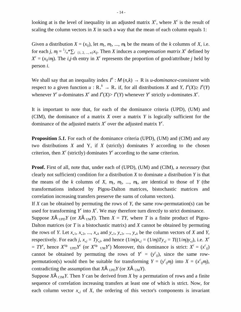
looking at is the level of inequality in an adjusted matrix Xc, where Xc is the result ofscaling the column vectors in X in such a way that the mean of each column equals 1:
Given a distribution X = (xij), let µ1, µ2, ..., µk be the means of the k columns of X, i.e.for each j, µj = 1/n*∑ i∈{1, 2, ..., n}xij. Then X induces a compensation matrix Xc defined byXc = (xij/µj). The i,j-th entry in Xc represents the proportion of good/attribute j held byperson i.
We shall say that an inequality index In : M (n,k) → R is u-dominance-consistent withrespect to a given function u : R+
k → R+ if, for all distributions X and Y, In(X)≥ In(Y)whenever Yc u-dominates Xc and In(X)> In(Y) whenever Yc strictly u-dominates Xc.
It is important to note that, for each of the dominance criteria (UPD), (UM) and(CIM), the dominance of a matrix X over a matrix Y is logically sufficient for thedominance of the adjusted matrix Xc over the adjusted matrix Yc.
Proposition 5.1. For each of the dominance criteria (UPD), (UM) and (CIM) and anytwo distributions X and Y, if X (strictly) dominates Y according to the chosencriterion, then Xc (strictly) dominates Yc according to the same criterion.
Proof. First of all, note that, under each of (UPD), (UM) and (CIM), a necessary (butclearly not sufficient) condition for a distribution X to dominate a distribution Y is thatthe means of the k columns of X, µ1, µ2, ..., µk, are identical to those of Y (thetransformations induced by Pigou-Dalton matrices, bistochastic matrices andcorrelation increasing transfers preserve the sums of column vectors).If X can be obtained by permuting the rows of Y, the same row-permutation(s) can beused for transforming Yc into Xc. We may therefore turn directly to strict dominance.Suppose XÂUPDY (or XÂUMY). Then X = TY, where T is a finite product of Pigou-Dalton matrices (or T is a bistochastic matrix) and X cannot be obtained by permutingthe rows of Y. Let x•1, x•2, ..., x•k and y•1, y•2, ..., y•k be the column vectors of X and Y,respectively. For each j, x•j = Ty•j, and hence (1/µj)x•j = (1/µj)Ty•j = T((1/µj)y•j), i.e. Xc
= TYc, hence XcºUPDYc (or XcºUMYc) Moreover, this dominance is strict: Xc = (xc
ij)cannot be obtained by permuting the rows of Yc = (yc
ij), since the same row-permutation(s) would then be suitable for transforming Y = (yc
ijµj) into X = (xcijµj),
contradicting the assumption that XÂUPDY (or XÂUMY).Suppose XÂCIMY. Then Y can be derived from X by a permutation of rows and a finitesequence of correlation increasing transfers at least one of which is strict. Now, foreach column vector x•j of X, the ordering of this vector's components is invariant
- 15 -
under multiplication by (1/µj), and hence Xc = (xij/µj) can be transformed into Yc =(yij/µj) by the same correlation increasing transfers (one of which is strict) and row-permutations by which X can be transformed into Y. Hence XcÂCIMYc. Q.E.D.
If X dominates Y according to (DM) (or (DM+)), on the other hand, this does not ingeneral imply that Xc also dominates Yc according to (DM) (or (DM+)). For instance,if Y=2X, then YÂDM+X, but Xc=Yc, whence it is not the case that YcÂDM+Xc. However,if our main focus is on the relative distribution of goods within each dimension ratherthan the total amount of goods in each dimension, we can use the following criteriainstead of (DM) and (DM+):
DIRECTIONAL/PRICE MAJORIZAION OF COMPENSATION MATRICES (DMC).(X,Y)∈DMC if and only if (Xc, Yc)∈DM.
DIRECTIONAL/PRICE MAJORIZAION OF COMPENSATION MATRICES (DM+C).(X,Y)∈DM+C if and only if (Xc, Yc)∈DM+.
Proposition 5.1. and the results of section 3. are easily seen to imply that
UPD ⊆ UM ⊂ DMC
⊂ DM+C (with UPD=UM whenever k≤2). CIM
But then proposition 5.1. and the results of section 4. imply that, whenever u : R+k →
R+ is continuous, increasing, strictly concave and of the form u(t) = f1(t1) + f2(t2) + ... +fk(tk), for all t∈R+
k, a u-dominance-consistent inequality index satisfies (UM)(including (UPD)), (CIM) and (DM+C) (including (DMC))6.
We will now define two u-dominance-consistent inequality indices satisfying (C), (A),(N), (RI), (RS), (UPD), (UM), (DMC), (DM+C) and (CIM).
The first one is a generalization of the well-known one-dimensional Gini coefficient.As before, let u(t) = ∑ j∈{1, 2, ..., k}tj
rj (with 0 < rj < 1, for each j).
First note the following lemma:
6Such an inequality index will not, in general, satisfy (DM) and (DM+). But if -- as
emphasized -- our focus is on relative distributions, rather than the total amounts, of goods,and if compensation matrices rather than unadjusted distribution matrices should thereforeform the basis for inequality comparisons, it is plausible (indeed requisite) to replace (DM)and (DM+) with (DMC) and (DM+C), respectively.
- 16 -
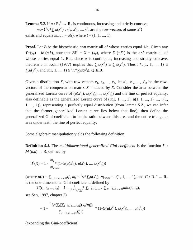
Lemma 5.2. If u : R+k → R+ is continuous, increasing and strictly concave,
max{1/n*∑ iu(xci) : xc
1, xc2, ..., xc
n are the row-vectors of some Xc}exists and equals µu-max = u(t), where t = (1, 1, ..., 1).
Proof. Let B be the bistochastic n×n matrix all of whose entries equal 1/n. Given anyY=(yij) ∈ M (n,k), note that BYc = X = (xij), where X (=Xc) is the n×k matrix all ofwhose entries equal 1. But, since u is continuous, increasing and strictly concave,theorem 3 in Kolm (1977) implies that ∑ iu(xc
i) ≥ ∑ iu(yci). Thus n*u(1, 1, ..., 1) ≥
∑ iu(yci), and u(1, 1, ..., 1) ≥ 1/n*∑ iu(yc
i). Q.E.D.
Given a distribution X, with row-vectors x1, x2, ..., xn, let xc1, xc
2, ..., xcn be the row-
vectors of the compensation matrix Xc induced by X. Consider the area between thegeneralized Lorenz curve of (u(xc
1), u(xc2), ..., u(xc
n)) and the line of perfect equality,also definable as the generalized Lorenz curve of (u(1, 1, ..., 1), u(1, 1, ..., 1), ..., u(1,1, ..., 1)), representing a perfectly equal distribution (from lemma 5.2., we can inferthat the former generalized Lorenz curve lies below that line); then define thegeneralized Gini-coefficient to be the ratio between this area and the entire triangulararea underneath the line of perfect equality.
Some algebraic manipulation yields the following definition:
Definition 5.3. The multidimensional generalized Gini coefficient is the function In :M (n,k) → R, defined by
Theorem 5.4. The multidimensional generalized Gini coefficient satisfies (C), (A),(N), (RI), (RS), (UPD), (UM), (DMC), (DM+C) and (CIM).
Proof. (C): Consider the formulation
µu In(X) = 1 - * (1-G(u(xc
1), u(xc2), ..., u(xc
n))), µu-max
and note that the function which maps each X to Xc and the functions which map eachXc to the vector (u(xc
1), u(xc2), ..., u(xc
n)) and to µu, and G are all continuous (and µu-max
is constant), and hence, by the chain rule for continuity, so is In.(A): Given an n×n permutation matrix Π permuting the rows of X, first note that (ΠX)c
= ΠXc. But now it is sufficient to observe that both µu = 1/n*∑ iu(xci) and G(u(xc
1),u(xc
2), ..., u(xcn)) are invariant under permutations of xc
1, xc2, ..., xc
n.(N): If all rows of a distribution X are identical, Xc is the matrix all of whose entriesequal 1. Then µu = µu-max and G(t, t, ..., t) = 0 with t = u(1, 1, ..., 1), whence In(X) = 0.(RI): Given a n×k matrix X, let Y be the n*r×k matrix defined by
XY = X (with r 'replications' of X),
(⋅⋅⋅) X
and first note that
Xc
Xc = Xc (with r 'replications' of Xc). (⋅⋅⋅ )
Xc
Now let yc1, yc
2, ..., ycr*n be the row-vectors of Yc; then, for each j∈{0, 1, ..., r-1} and
each i∈{1, 2, ..., n}, ycj*n+i = xc
i, and
1/r*n*∑ i∈{1, ..., r*n}u(yci)
Ir*n(Y) = 1 - * (1-G(u(yc1), u(yc
2), ..., u(ycr*n))), ∑ j∈{1, 2, ..., k}fj(1)
- 18 -
1/n*r*(r*∑ i∈{1, ..., n}u(xci))
= 1 - * (1-G(u(xc1), u(xc
2), ..., u(xcn))),
∑ j∈{1, 2, ..., k}fj(1)
(since G is replication invariant -- see Sen (1997), pp. 139 / 140)
= In(X).(RS): It is sufficient to observe that, for any n×n diagonal matrix Λ=diag(λ1, λ2, ..., λn)(with each λi>0), (ΛX)c = Xc.To prove that In satisfies (UPD), (UM), (DMC), (DM+C) and (CIM), it is sufficient toprove that In is u-dominance-consistent. Given our definition of u, In will then satisfy(DM+C), including (DMC), (UM), (UPD) and (CIM), as established above. But it isknown that, for any s = (s1, s2, ..., sn), t = (t1, t2, ..., tn) ∈ Rn, whenever s GL-dominatest, (1/n*∑ isi)*(1-G(s1, s2, ..., sn)) ≥ (1/n*∑ iti)*(1-G(t1, t2, ..., tn)) ('>' if the dominance isstrict) (see Sen (1997), pp. 136 / 137). This implies that 1/n*∑ iu(xc
i)*(1-G(u(xc
1),u(xc2),...,u(xc
n))) ≥ 1/n*∑ iu(yci)*(1-G(u(yc
1),u(yc2),...,u(yc
n))) whenever Xc u-dominates Yc ('>' if the u-dominance is strict); and hence In(X)≤ In(Y) whenever Xc u-dominates Yc ('>' if the u-dominance is strict). Thus In is u-dominance-consistent asrequired. Q.E.D.
The second u-dominance-consistent inequality index to be defined can be interpretedas a generalization of Atkinson's one-dimensional measure of inequality. In thepresent case, the idea is to define a social evaluation function W which maps eachcompensation matrix Xc to an 'equally distributed equivalent compensation figure', i.e.a strictly positive real number µe such that W(Xc) = µe = W(Y), where Y is the n×kmatrix all of whose entries equal µe. The overall level of inequality under adistribution X is then identified with the normalized difference between the 'equallydistributed equivalent compensation figure' of a perfectly equal distribution and the'equally distributed equivalent compensation figure' of Xc.
The function W will be required to be a suitable 'social extension' of the (personal)aggregation function u : R+
k → R+. Define W : M (n,k) → R+ as follows. This time, letu(t) = ∑ j∈{1, 2, ..., k}tj
r (with 0 < r < 1). Given a distribution matrix X with row-vectors x1,x2, ..., xn, let
where 0 < r, s < 1. Then W satisfies the demanded properties: in particular, for anymatrix X, W(X) = µe = W(Y), where Y is the n×k matrix all of whose entries equal µe.
- 19 -
Before we can define the inequality index, we need to state two lemmas:
Lemma 5.5. If w : R+ → R+ is continous, increasing and strictly concave and C is afixed strictly positive constant,
max{1/n*∑ iw(ti) : t = (t1, t2, ..., tn) ∈ R+n, where ∑ iti ≤ C}
exists and equals w(C/n).
Proof. Let B be the bistochastic n×n matrix all of whose entries equal 1/n. Given any t= (t1, t2, ..., tn) such that ∑ iti ≤ C, let ε = (C-∑ iti)/n, and let t' = (t'1, t'2, ..., t'n) with t'i =ti+ε. Then ∑ it'i = C, and since w is increasing, 1/n*∑ iw(t'i) ≥ 1/n*∑ iw(ti). Note that B(t'1,t'2, ..., t'n)=(C/n, C/n, ..., C/n), where the vectors are interpreted as column vectors. Butsince w is continuous, increasing and strictly concave, standard results (e.g. Sen, 1997,theorem 3.1) imply that ∑ iw(C/n) ≥ ∑ iw(t'i), and therefore w(C/n) = 1/n*∑ iw(C/n) ≥1/n*∑ iw(t'i) ≥ 1/n*∑ iw(ti). Q.E.D.
Lemma 5.6. Wmax:= max{W(Xc) : Xc is a compensation matrix} = 1.
Proof. By lemma 5.2.,
max{∑ iu(xci) : xc
1, xc2, ..., xc
n are the row-vectors of some Xc}= u(1, 1, ..., 1) = n*k,
whence, by lemma 5.5.,
max{1/n*∑ iu(xci)s : xc
1, xc2, ..., xc
n are the row-vectors of some Xc}= max{1/n*∑ iw(ti) : t = (t1, t2, ..., tn) ∈ R+
n, where ∑ iti ≤ n*k}= (n*k/n)s = ks, (with w(t) = ts)
and some easy manipulation yields the desired result. Q.E.D.
Lemma 5.6. confirms our intuition that the maximal value attained by the function Wfor some compensation matrix Xc equals 1, which is the 'equally distributed equivalentcompensation figure' of the matrix all of whose entries equal µ1 = µ2 = ... = µk = 1.
Definition 5.7. A multidimensional generalization of Atkinson's one-dimensionalinequality index is given by the function In : M (n,k) → R, where
Theorem 5.8. The above defined multidimensional generalization of Atkinson's one-dimensional inequality index satisfies (C), (A), (N), (RI), (RS), (UPD), (UM), (DMC),(DM+C) and (CIM).
and note that the function which maps each X to Xc, as well as all other 'components'of this function are themselves continuous functions; by the chain rule for continuity,In is continuous.(A): The invariance of In under permutations of the row-vectors x1, x2, ..., xn,equivalent to permutations of the n terms (1/k*∑ j∈{1, 2, ..., k}(xij/µj)r), is obvious.(N): If all rows of a distribution X are identical, again note that Xc is the matrix all ofwhose entries equal 1. But we have seen above that, in this case, W(Xc) = 1, and henceIn(X) = 0.(RI): Given a n×k matrix X, define Y and Yc as in the proof of theorem 5.4. (just use pinstead of r to denote the number of replications of X). Then
(RS): As before, it is sufficient to observe that, for any n×n diagonal matrixΛ=diag(λ1, λ2, ..., λn) (with each λi>0), (ΛX)c = Xc.To prove that In satisfies (UM), (UPD), (DM+C), (DMC) and (CIM), it is againsufficient to prove that In is u-dominance-consistent. First define E : R+
n → R+ be thefunction
E(t) = 1/n*∑ itis, with 0 < s < 1.
Now a result by Shorrocks (1983) implies that, since E(t) is symmetric, replicationinvariant, increasing, strictly concave, and additive, the following holds: for any s, t ∈R+
n, E(s) ≥ E(t) whenever s GL-dominates t ('>' if the dominance is strict). But thismeans that 1/n*∑ iu(xc
dominates Yc ('>' if the dominance is strict), and thus In is u-dominance consistent.Q.E.D.
- 21 -
6. Conclusion
In the present paper, I have first surveyed a number of dominance criteria representingdifferent answers to the question of when one multidimensional distribution is moreunequal than another: uniform Pigou-Dalton majorization (UPD), uniformmajorization (UM), directional/price majorization (DM(c)), non-negativedirectional/price majorization (DM+(c)) and correlation increasing majorization (CIM),and I have shown that they are logically interrelated in the following way ("⊆" ("⊂ ")means "is a (proper) subrelation of"):
UPD ⊆ UM ⊂ DM(c)
⊂ DM+(c) (with UPD=UM whenever k≤2). CIM
It is important to note that, whilst (UPD), (UM) and (DM(c)) are sensitive to theuniform inequality of a multidimensional distribution across people, only (CIM) and,as I have shown, (DM+(c)) are sensitive to the cross-correlation between inequalitiesin different dimensions.
I have secondly proposed a new method of constructing multidimensional inequalityindices. Given a multidimensional distribution matrix (subsequently normalized suchthat the mean of each column, i.e. dimension of goods/attributes, equals 1), the firststep is to use a suitable function u : R+
k → R+ to aggregate each person's row-vector ofgoods/attributes into an overall evaluation figure for this person (representing howwell-off this person is in terms of his or her share of goods across the differentdimensions) and thus to transform a multidimensional distribution into a one-dimensional distribution of evaluation figures. The second step is to note that, for ourdefinition of u, the generalized Lorenz ordering of these one-dimensional distributionsof evaluation figures respects all of the dominance criteria (for the originalmultidimensional distributions) surveyed above. The third step is to define amultidimensional inequality index (and thereby to extend the dominance-inducedpartial orderings on the set of all multidimensional distributions to a completeordering) by using a suitable generalized-Lorenz-consistent aggregation function tomap each one-dimensional distribution of evaluation figures to a single real number,representing the overall level of inequality in the given multidimensional distribution.
To illustrate the proposed method, I have defined two new classes ofmultidimensional inequality indices:
- 22 -
(a) a multidimensional generalization of the Gini-coefficient: for each distribution X = (xij) ∈ M (n,k) with column means µ1, µ2, ..., µk,
(b) a multidimensional generalization of Atkinson's one-dimensional inequality index: for each distribution X = (xij) ∈ M (n,k) with column means µ1, µ2, ..., µk,
Both (a) and (b) satisfy continuity, anonymity, normalization (in fact, they always takevalues in the interval [0, 1]), replication invariance and ratio-scale invariance.Moreover, they respect all of (UM), (UPD), (DMC), (DM+C) and (CIM) and therebycapture both Kolm's and Atkinson, Bourguignon and Walzer's intuitions aboutmultidimensional inequality: firstly, they are sensitive to how uniformly unequal thedistribution of goods/attributes across people is (by virtue of satisfying (UPD), (UE)and (DMC)), and, secondly, they are sensitive to how systematically inequalities indifferent dimensions are cross-correlated (by virtue of satisfying (CIM) and (DM+C)).
The results of this paper may thus point towards new ways of operationalizing theideas pioneered by Kolm (1977), Atkinson and Bourguignon (1982) and Walzer(1983).
Bibliography
Atkinson, A. B.: "On the Measurement of Inequality", Journal of Economic Theory, 2,1970, pp. 244 - 263
Atkinson, A. B., & Bourguignon, F.: "The Comparison of Multi-DimensionedDistributions of Economic Status", Review of Economic Studies, XLIX,1982, pp. 183 - 201
Bhandari, K. S.: "Multivariate majorization and directional majorization: negativeresults", Calcutta-Statistical-Association-Bulletin, 45, 1995, no. 179-180,pp. 149-159
- 23 -
Boland, P., & Proschan, F.: "Multivariate arrangement increasing functions withapplication in probability and statistics", Journal of Multivariate Analysis, 25,1988, pp. 286 - 298
Fisher, F. M.: "Income Distribution, Value Judgements and Welfare", QuarterlyJournal of Economics, 70, 1956, pp. 380 - 424
Kolm, S.-C.: "Multidimensional Egalitarianisms", Quarterly Journal of Economics,XCI, 1, 1977, pp. 1 - 13
Koshevoy, G., & Mosler, K.: "Multivariate Gini indices", Journal of MultivariateAnalysis, 60, 1997, pp. 252 - 276
Maasoumi, E.: "The measurement and decomposition of multi-dimensionalinequality", Econometrica, 54, 1986, pp. 771 - 779
Marshall, A. W., & Olkin, I.: Inequalities: theory of majorization and its applications,San Diego (Academic Press), 1979
Sen, A.: On Economic Inequality, 2nd ed., Oxford (Oxford University Press), 1997Shorrocks, A. F.: "Ranking Income Distributions", Economica, 50, 1983, pp. 3 - 17Tsui, K.-Y.: "Multidimensional generalizations of the relative and absolute inequality
indices: the Atkinson-Kolm-Sen approach", Journal of Economic Theory, 67,1995, pp. 251 - 265
Tsui, K.-Y.: "Multidimensional inequality and multidimensional generalized entropymeasures: An axiomatic derivation", Social Choice and Welfare, 16, 1999,pp. 145 - 157
Walzer, M.: Spheres of Justice, New York (Basic Books), 1983