Acta Math. Hungar., 136 (3) (2012), 196–221 DOI: 10.1007/s10474-012-0217-4 First published online April 3, 2012 MULTIGRAPH LIMIT OF THE DENSE CONFIGURATION MODEL AND THE PREFERENTIAL ATTACHMENT GRAPH B. R ´ ATH 1,∗ and L. SZAK ´ ACS 2 1 ETH Z¨ urich, Department of Mathematics, R¨ amistrasse 101, 8092 Z¨ urich, Switzerland e-mail: [email protected]2 E¨ otv¨ os Lor´and University, Institute of Mathematics, P´ azm´ any P´ eter s´ et´ any 1/C, 1117 Budapest, Hungary e-mail: [email protected](Received June 23, 2011; revised November 21, 2011; accepted November 23, 2011) Abstract. The configuration model is the most natural model to gener- ate a random multigraph with a given degree sequence. We use the notion of dense graph limits to characterize the special form of limit objects of convergent sequences of configuration models. We apply these results to calculate the limit object corresponding to the dense preferential attachment graph and the edge re- connecting model. Our main tools in doing so are (1) the relation between the theory of graph limits and that of partially exchangeable random arrays (2) an explicit construction of our random graphs that uses urn models. 1. Introduction The notion of dense graph limits was introduced in [10] and has been further developed over the years, see [9] for a recent survey. Heuristically, the theory of dense graph limits gives a compact way to characterize the statistics of a randomly chosen small subgraph of a large dense graph. In [5] the graph limits of various sequences of random dense graphs were calculated and in this paper we proceed with the investigation of this topic. Our objects of study are multigraphs rather than simple graphs, i.e. we allow parallel and loop edges: this choice makes the definition of the limit objects of convergent multigraph sequences (multigraphons ) slightly more complicated than the limit objects of simple graph sequences (graphons), but on the other hand the multigraph models defined below are easier to study than the corresponding simple graph models. ∗ Corresponding author. Key words and phrases: dense graph limit, multigraph, configuration model, preferential at- tachment. Mathematics Subject Classification: 05C80. 0236-5294/$ 20.00 c 2012 Akad´ emiai Kiad´o, Budapest, Hungary
(Received June 23, 2011; revised November 21, 2011; accepted November 23, 2011)
Abstract. The configuration model is the most natural model to gener-ate a random multigraph with a given degree sequence. We use the notion ofdense graph limits to characterize the special form of limit objects of convergentsequences of configuration models. We apply these results to calculate the limitobject corresponding to the dense preferential attachment graph and the edge re-connecting model. Our main tools in doing so are (1) the relation between thetheory of graph limits and that of partially exchangeable random arrays (2) anexplicit construction of our random graphs that uses urn models.
1. Introduction
The notion of dense graph limits was introduced in [10] and has beenfurther developed over the years, see [9] for a recent survey. Heuristically,the theory of dense graph limits gives a compact way to characterize thestatistics of a randomly chosen small subgraph of a large dense graph. In [5]the graph limits of various sequences of random dense graphs were calculatedand in this paper we proceed with the investigation of this topic.
Our objects of study are multigraphs rather than simple graphs, i.e. weallow parallel and loop edges: this choice makes the definition of the limitobjects of convergent multigraph sequences (multigraphons) slightly morecomplicated than the limit objects of simple graph sequences (graphons),but on the other hand the multigraph models defined below are easier tostudy than the corresponding simple graph models.
∗ Corresponding author.Key words and phrases: dense graph limit, multigraph, configuration model, preferential at-
MULTIGRAPH LIMIT OF THE DENSE CONFIGURATION MODEL 197
The simplest way to generate a random multigraph with a prescribeddegree sequence is called the configuration model: we draw d(v) stubs (half-edges) at each vertex v and then we uniformly choose one from the setof possible matchings of these stubs. In this paper we call such randommultigraphs edge stationary (for reasons that will become clear later) and inTheorem 1 we characterize the special form of limiting multigraphons thatarise as the limit of random dense edge stationary multigraph sequences.Rougly speaking, our theorem states that the number of edges connectingthe vertices v and w has Poisson distribution with parameter proportionalto d(v)d(w).
We also investigate two random graph models which have different defi-nitions but turn out to have the same distribution:
• The edge reconnecting model is a random multigraph evolving in time.Denote the multigraph at time T by Gn(T ), where T = 0, 1, 2, . . . and n =
|V (Gn(T )
) | is the number of vertices. We denote by m = |E(Gn(T )
) | thenumber of edges (the number of vertices and edges does not change overtime). Given the multigraph Gn(T ) we get Gn(T + 1) by uniformly choosingan edge in E
(Gn(T )
), choosing one of the endpoints of that edge with a coin
flip and reconnecting the edge to a new endpoint which is chosen using therule of linear preferential attachment: a vertex v is chosen with probabilityd(v)+κ2m+nκ , where d(v) is the degree of vertex v in Gn(T ) and κ ∈ (0,+∞) isa fixed parameter of the edge reconnecting model. We look at the uniquestationary distribution of this multigraph-valued Markov chain which is arandom multigraph on n vertices and m edges.
• In Section 3.4 of [5] a random multigraph called preferential attachmentgraph with n nodes and m edges (briefly PAG(n,m)) is defined. We slightlygeneralize the definition to obtain PAGκ(n,m) where κ ∈ (0,+∞) is a fixedparameter: let V = {v1, . . . , vn} be a set of vertices. We create a sequencev∗1, . . . , v
∗2m with elements from V by starting with the empty sequence and
appending random elements of V one by one. If the current length of thesequence is L then we choose the next element v∗
L+1 to be equal to v ∈ V
with probability d(v)+κL+nκ , where d(v) is the multiplicity of v in the sequence
v∗1, . . . , v
∗L. Now we create the random multigraph PAGκ(n,m) on the vertex
set V by adding the edges of form {v∗2k−1, v
∗2k } for each k = 1, . . . , m.
Lemma 2.1 states that the above described two random multigraphs havethe same distribution. In Theorem 2 we give the limiting multigraphon ofthis random multigraph when n → ∞ and m ≈ 1
2ρn2, where ρ ∈ (0,+∞) is afixed parameter of the model called the edge density. Roughly speaking, thelimiting multigraphon can be described as follows: it is edge stationary, andthe rescaled degrees of vertices have Gamma distribution with parametersdepending on κ and ρ.
Acta Mathematica Hungarica 136, 2012
198 B. RATH and L. SZAKACS
The precise statements of these theorems along with the necessary nota-tions can be found in Section 2. We end the Introduction with mentioninga few related results:
The configuration model is a random multigraph, but if we condition itto have no multiple and loop edges, then the resulting random simple graphis uniformly distributed given its degree sequence. In [6] the descriptionof the limiting graphon of such sequences of simple dense graphs (and acontinuous version of the Erdos–Gallai characterization of degree sequences)is given.
In [13] we give a characterization of the time evolution of the edge re-connecting model, viewed through the prism of the theory of multigraphons:roughly speaking, if we start the edge reconnecting model from an arbitraryinitial multigraph, then we have to run our process for n2 � T steps untilGn(T ) becomes “edge stationary” and run it for n3 � T steps until Gn(T )becomes “stationary”.
Acknowledgement. The authors thank Laszlo Lovasz for posing theresearch problem that became the subject of this paper. The research ofBalazs Rath was partially supported by the OTKA (Hungarian NationalResearch Fund) grants K 60708 and CNK 77778, Morgan Stanley AnalyticsBudapest and Collegium Budapest and the grant ERC-2009-AdG 245728-RWPERCRI. The research of Laszlo Szakacs was partially supported by theOTKA grant NK 67867.
2. Notation and results
Denote N0 = {0, 1, 2, . . . }, [n] := {1, . . . , n} and [k..n] := {k, . . . , n}. IfH1 and H2 are arbitrary sets, denote by f : H1 ↪→ H2 a generic injectivefunction from H1 to H2. Denote by M the set of undirected multigraphs(graphs with multiple and loop edges) and by Mn the set of multigraphson n vertices. Let G ∈ Mn. The adjacency matrix of a labeling of themultigraph G with [n] is denoted by
(B(i, j)
)n
i,j=1, where B(i, j) ∈ N0 is the
number of edges connecting the vertices labeled by i and j. B(i, j) = B(j, i)since the graph is undirected and B(i, i) is twice the number of loop edgesat vertex i (thus B(i, i) is an even number).
Denote the set of adjacency matrices of multigraphs on n nodes by An,thus
An ={
B ∈ Nn×n0 : BT = B, ∀ i ∈ [n] 2 | B(i, i)
}.
The degree of the vertex labeled by i in G with adjacency matrix B ∈ An
is defined by d(B, i) :=∑n
j=1 B(i, j), thus d(B, i) is the number of stubs at i
Acta Mathematica Hungarica 136, 2012
MULTIGRAPH LIMIT OF THE DENSE CONFIGURATION MODEL 199
(loop edges count twice). Let
m = m(G) = m(B) =12
n∑
i,j=1
B(i, j) =12
n∑
i=1
d(B, i)
denote the number of edges. Denote by Amn the set of adjacency matrices
on n vertices with m edges.An unlabeled multigraph is the equivalence class of labeled multigraphs
where two labeled graphs are equivalent if one can be obtained by relabel-ing the other. Thus M is the set of these equivalence classes of labeledmultigraphs, which are also called isomorphism types.
Suppose F ∈ Mk, G ∈ Mn and denote by A ∈ Ak and B ∈ An the adja-cency matrices of F and G. If g : M → R then we say that g is a multigraphparameter. Let g(A) := g(F ). Conversely, if g :
⋃∞k=1 Ak → R is constant
on isomorphism classes, then g defines a multigraph parameter.
2.1. Multigraphons and multigraph convergence. We define theinduced homomorphism density of F into G by
t=(F, G) := t=(A,B) :=1nk
∑
ϕ: [k]→[n]
11[∀ i, j ∈ [k] : A(i, j) = B(ϕ(i), ϕ(j)
)].
(1)
The notion of convergence of simple graph sequences and several equiv-alent characterizations of graphons (limit objects of convergent graph se-quences) were given in [10]. In [8] a natural generalization of the theory ofdense graph limits to multigraphs is given (see also [12] for similar resultsin a more general setting). We say that a sequence of multigraphs (Gn)∞
n=1is convergent if for every k ∈ N and every multigraph F ∈ Mk the limitg(F ) = limn→∞ t=(F,Gn) exists, moreover we have
∑A∈ Ak
g(A) = 1. Thelimit object of a convergent multigraph sequence is a measurable functionW : [0, 1] × [0, 1] × N0 → [0, 1] satisfying
(2) W (x, y, k) ≡ W (y, x, k),∞∑
k=0
W (x, y, k) ≡ 1, W (x, x, 2k + 1) ≡ 0.
Such functions are called multigraphons. For every multigraphon W andmultigraph F ∈ Mk with adjacency matrix A ∈ Ak define
(3) t=(F,W ) := t=(A,W ) :=∫
[0,1]k
∏
i�j�k
W(xi, xj ,A(i, j)
)dx1 dx2 . . . dxk.
Acta Mathematica Hungarica 136, 2012
200 B. RATH and L. SZAKACS
We say that Gn → W if for every k ∈ N and every F ∈ Mk we havelimn→∞ t=(F, Gn) = t=(F,W ). Theorem 1 of [8] states that if a sequenceof multigraphs (Gn)∞
n=1 is convergent then Gn → W for some multigraphonW and conversely, every multigraphon W arises this way. The limitingmultigraphon of a convergent sequence is not unique, but if we define theequivalence relation W1
∼= W2 by ∀ F ∈ M : t=(F,W1) = t=(F,W2) then ob-viously Gn → W1, Gn → W2 implies W1
∼= W2. For other characterisationsof the equivalence relation ∼= for graphons, see [4].
For a multigraphon W and x ∈ [0, 1] define the average degree of W at xand the edge density of W by
D(W,x) :=∫ 1
0
∞∑
k=0
k · W (x, y, k) dy,(4)
ρ(W ) :=∫ 1
0
∫ 1
0
∞∑
k=0
k · W (x, y, k) dy dx.(5)
If ρ(W ) < +∞ then D(W,x) < +∞ for Lebesgue-almost all x.Given a multigraphon W define the degree distribution function of W by
(6) FW (z) =∫ 1
011
[D(W,x) � z
]dx, z � 0.
Indeed, FW (·) is a probability distribution function on [0, ∞), i.e. it is non-negative, right continuous, increasing and satisfies limz→∞ FW (z) = 1. It iseasy to see that ρ(W ) =
∫ ∞0 z dFW (z). Denote
(7) F −1W (u) := min
{z : FW (z) � u
}, u ∈ (0, 1).
2.2. Random multigraphs and random adjacency matrices. De-note a random element of An by Xn. We may associate a random multi-graph Gn to Xn by taking the isomorphism class of Xn.
We say that a sequence of random multigraphs (Gn)∞n=1 converges in
probability to a multigraphon W (or briefly write Gnp−→ W ) if for every
multigraph F we have t=(F, Gn)p−→ t=(F,W ), i.e.
(8) ∀ F ∈ M ∀ ε > 0 : limn→∞
P(∣∣ t=(F, Gn) − t=(F,W )
∣∣ > ε) = 0.
We say that Xnp−→ W if Gn
p−→ W holds for the associated random multi-graphs.
Note that the definitions of the edge reconnecting model and the PAGκ
(see Section 1) in fact naturally give rise to a random labeled graph, i.e.
Acta Mathematica Hungarica 136, 2012
MULTIGRAPH LIMIT OF THE DENSE CONFIGURATION MODEL 201
a random element Xn of An. The edge reconnecting Markov chain is eas-ily seen to be irreducible and aperiodic on the state space Am
n , thus thestationary distribution is indeed unique.
We say that the distribution of Xn is edge stationary if the conditionaldistribution of Xn given the degree sequence
(d(Xn, i)
)n
i=1is the same as
that of the configuration model (see Section 1) with the same degree se-quence.
Recall the formulas defining the Poisson and Gamma distributions:
p(k, λ) := e−λ λk
k!(9)
g(x, α, β) := xα−1 βαe−βx
Γ(α)11[x > 0].(10)
We say that a nonnegative integer-valued random variable X has Poissondistribution with parameter λ (or briefly denote X ∼ POI (λ)) if P(X = k)= p(k, λ) for all k ∈ N. We say that a nonnegative real-valued random vari-able Z has gamma distribution with parameters α and β (or briefly denoteZ ∼ Gamma (α, β)) if P(Z � z) =
∫ z0 g(x, α, β) dx.
For a real-valued nonnegative random variable X define
E(X;m) := E(X · 11[X � m]
).
2.3. Statements of main results. First we state our theorem char-acterizing the form of multigraph limits of edge stationary multigraph se-quences:
Theorem 1. Let W denote a multigraphon with ρ(W ) < +∞. If Xn isan An-valued edge stationary random variable for all n ∈ N, Xn
p−→ W forsome multigraphon W , and the sequence (Xn)∞
n=1 satisfies
limm→∞
supn∈N
1(n2
)∑
i<j�n
E(Xn(i, j);m
)= 0(11)
limm→∞
supn∈N
1n
n∑
i=1
E(Xn(i, i);m
)= 0,(12)
Acta Mathematica Hungarica 136, 2012
202 B. RATH and L. SZAKACS
then the limiting multigraphon W can be rewritten in the form W ∼= W where
(13) W (x, y, k)(7),(9):=
⎧⎪⎪⎪⎪⎪⎨
⎪⎪⎪⎪⎪⎩
p
(
k,F −1
W (x)F −1W (y)
ρ(W )
)
if x = y,
11[2 | k] · p
(k
2,F −1
W (x)F −1W (y)
2ρ(W )
)
if x = y.
Now we state our results describing the multigraph limit of thePAGκ(n,m) and the stationary distribution of the edge reconnecting model.
For an adjacency matrix B ∈ An denote by m′(B) =∑n
i=1
∑i−1j=1 B(i, j)
the number of non-loop edges of the corresponding graph.
Lemma 2.1. The unique stationary distribution of the edge reconnectingmodel with linear preferential attachment parameter κ and state space Am
n
has the same distribution as PAGκ(n,m). If Xn has this distribution thenfor all B ∈ Am
n
P(Xn = B) =
∏ni=1
∏d(B,i)j=1 (κ + j − 1)
∏2mj=1(κn + j − 1)
m!2m′(B)
(∏n
i=1
∏i−1j=1 B(i, j)!)(
∏ni=1
B(i,i)2 !)
.
(14)
At the end of Section 3.4 of [5] the following theorem is stated:Let SPAG (n,m) denote the simple graph obtained from PAG (n,m) by
deleting loops and keeping only one copy of the parallel edges. Then
SPAG(
n,n2
2·(ρ + o(1)
))p−→ Ws,(15)
Ws(x, y) := 1 − exp(
− ρ ln (x) ln (y)),
where (analogously to (8)) the symbolp−→ denotes convergence in probabil-
ity of a sequence of random simple graphs to a (simple) graphon.It is easy to see that (15) is a corollary of the following theorem:
Theorem 2. Let us fix κ, ρ ∈ (0,+∞). If Xn is a random element ofAm(n)
n with distribution (14) for n = 1, 2, . . . , moreover the asymptotic edgedensity is
limn→∞
2m(n)n2
= ρ,
Acta Mathematica Hungarica 136, 2012
MULTIGRAPH LIMIT OF THE DENSE CONFIGURATION MODEL 203
then Xnp−→ W where
(16) W (x, y, k) =
⎧⎪⎪⎪⎨
⎪⎪⎪⎩
p(
k,F −1(x)F −1(y)
ρ
)if x = y
11[2|k] · p(
k
2,F −1(x)F −1(y)
2ρ
)if x = y
and F −1 is the inverse function of F (z) =∫ z0 g(y, κ, κ
ρ) dy, see (10).
Note the similarity of the multigraphons appearing in (13) and (16): aswe will see later, this is a consequence of the fact that the distribution ofPAGκ(n, m) is edge stationary.
The proofs of the above stated theorems rely on the following ideas:• We relate our random graph models to urn models with multiple colors
(e.g. the well-known Polya urn model): the number of balls is 2m and theyare colored with n possible colors. Each ball corresponds to a stub, eachcolor corresponds to a labeled vertex and the edge set of the multigraphdepends on the positions of balls in the urn.
• We make use of the underlying symmetries of the distributions of ourrandom graphs by relating the theory of graph limits to the theory of par-tially exchangeable arrays of random variables, a connection first observedin [7].
The rest of this paper is organized as follows. In Section 3 we introducethe notion of random, vertex exchangeable, infinite adjacency matrices aswell as W -random multigraphons and deduce some useful results relatingthe convergence of these objects to graph limits. In Section 4 we relate thenotion of edge stationarity to the ball exchangeability of the correspondingurn models and prove the convergence results stated above.
3. Vertex exchangeable arrays
In this section we introduce random infinite arrays X =(X(i, j)
) ∞i,j=1
that arise as the adjacency matrices of random infinite labeled multigraphsand give probabilistic meaning to the homomorphism densities t=(F,W ) byintroducing W -random infinite multigraphs XW . We also introduce the no-tion of the average degree D(X, i) of a vertex i in an infinite, dense, vertexexchangeable multigraph.
In Subsection 3.1 we give a useful alternative characterisation ofGn
p−→ W using exchangeable arrays and prove that under certain tech-nical conditions the average degrees of Gn converge in distribution to theaverage degrees D(XW , i) of the limiting W -random infinite array.
Acta Mathematica Hungarica 136, 2012
204 B. RATH and L. SZAKACS
Let AN denote the set of adjacency matrices(A(i, j)
) ∞i,j=1
of countablemultigraphs:
AN ={
A ∈ NN×N
0 : ∀ i, j ∈ N A(i, j) ≡ A(j, i), ∀ i ∈ N 2 | A(i, i)}
.
Consider the probability space (AN, F ,P) where F is the coarsest sigma-algebra with respect to which A(i, j) is measurable for all i, j and P is aprobability measure on the measurable space (AN, F ). We are going to de-note the infinite random array with distribution P by X =
(X(i, j)
) ∞i,j=1
.We use the standard notation X ∼ Y if X and Y are identically distributed(i.e. their distribution P is identical on (AN, F )).
If X is a random element of AN, let X[k] be the random element of Ak
defined by X[k] :=(X(i, j)
)k
i,j=1.
Definition 3.1 (W -random infinite multigraphons). Let (Ui)∞i=1 be
independent random variables uniformly distributed in [0, 1]. Given amultigraphon W define the random countable adjacency matrix XW =(XW (i, j)
) ∞i,j=1
as follows: Given the background variables (Ui)∞i=1 the ran-
dom variables(XW (i, j)
)i�j∈N
are conditionally independent and
P(XW (i, j) = m | (Ui)
∞i=1
)= W (Ui, Uj ,m),
that is if A ∈ Ak then we have
(17) P(X[k]W = A | (Ui)
∞i=1) :=
∏
i�j�k
W(Ui, Uj , A(i, j)
).
In plain words: if i = j and Ui = x, Uj = y then the number of multi-ple edges between the vertices labeled by i and j in XW has distribution(W (x, y, k)
) ∞k=1
and the number of loop edges at vertex i has distribution(W (x, x, 2k)
) ∞k=1
(these are indeed proper probability distributions by (2)).For every multigraphon W and multigraph F ∈ Mk with adjacency ma-
If ρ(W ) < +∞ then D(W,U1) < +∞ almost surely.We say that a random infinite array X =
(X(i, j)
) ∞i,j=1
is vertex ex-changeable if
(20) (X(τ(i), τ(j)
))
∞i,j=1
∼(X(i, j)
) ∞i,j=1
Acta Mathematica Hungarica 136, 2012
MULTIGRAPH LIMIT OF THE DENSE CONFIGURATION MODEL 205
for all finitely supported permutations τ : N → N. We call X =(X(i, j)
) ∞i,j=1
dissociated if for all m,n ∈ N the An-valued random variable(X(i, j)
)n
i,j=1is independent of the Am-valued random variable
(X(i, j)
)n+m
i,j=n+1.
In our case an infinite exchangeable array can be thought of as the ad-jacency matrix of a random multigraph with vertex set N: the adjacencymatrix of this random infinite multigraph is vertex exchangeable if and onlyif the distribution of the random graph is invariant under the relabeling ofthe vertices and dissociated if and only if subgraphs spanned by disjointvertex sets are independent.
It follows from Definition 3.1 that XW is vertex exchangeable and dis-sociated and by Aldous’ representation theorem (see Theorem 1.4, Proposi-tion 3.3 and Theorem 5.1 in [1]), the converse holds: a random element Xof AN is vertex exchangeable and dissociated if and only if X ∼ XW forsome multigraphon W . Although the notion of the W -random graph (seeDefinition 3.1) is already present in [10], the connection of Aldous’ represen-tation theorem with the theory of graph limits was first observed in [7]. Seealso Theorem 3.1, Theorem 3.2, Proposition 3.4 of [11]. For a self-containedproof of this representation theorem for multigraphons, see Theorem 1 andTheorem 2 in [8].
For a vertex exchangeable infinite array X satisfying E(X(1, 2)
)< +∞
define the average degree of X at vertex i by
(21) D(X, i) := limn→∞
1n
n∑
j=1
X(i, j).
The sum 1n
∑nj=1 X(i, j) indeed almost surely converges to a random variable
as n → ∞ by de Finetti’s theorem (see Section 2.1 of [2]) and the conditionalstrong law of large numbers. From (4), Definition 3.1 and (19) we get
(22) D(XW , i) = limn→∞
1n
n∑
j=1
XW (i, j) a.s.= D(W, Ui).
3.1. Convergence of exchangeable arrays. In this subsection westate and prove two lemmas: in Lemma 3.1 we relate convergence of denserandom multigraphs to convergence of the probability measures of the cor-responding random arrays, and in Lemma 3.2 we give sufficient conditionsunder which convergence of dense random multigraphs imply convergence ofthe degree distribution of these graphs.
We say that a sequence of random infinite arrays (Xn)∞n=1 converges in
distribution to a random infinite array X (or briefly denote Xnd−→ X) if
Acta Mathematica Hungarica 136, 2012
206 B. RATH and L. SZAKACS
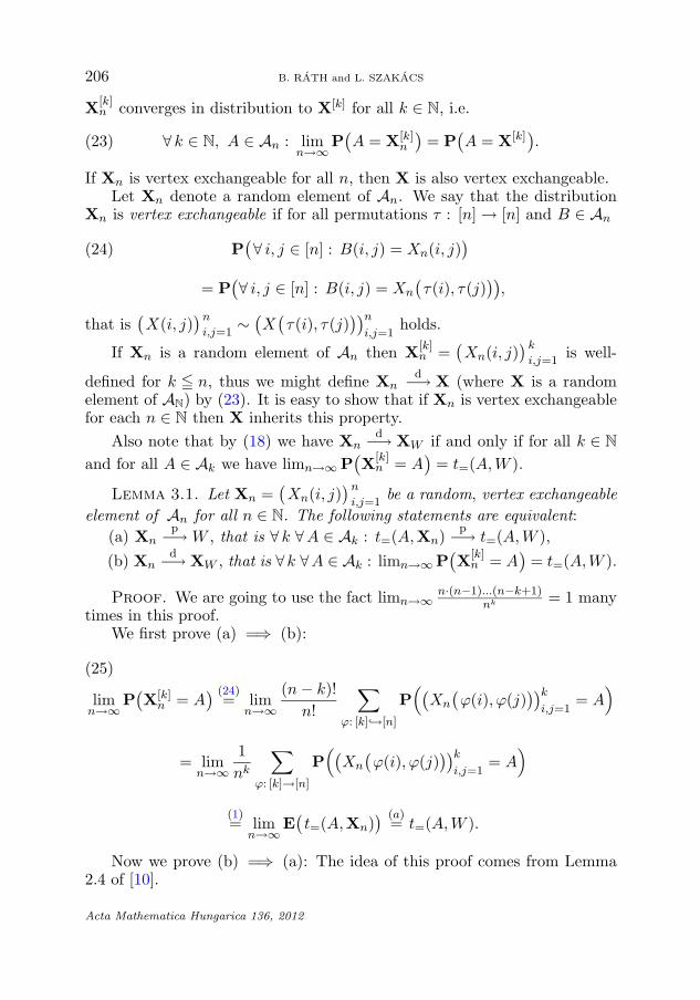
X[k]n converges in distribution to X[k] for all k ∈ N, i.e.
(23) ∀ k ∈ N, A ∈ An : limn→∞
P(A = X[k]n ) = P(A = X[k]).
If Xn is vertex exchangeable for all n, then X is also vertex exchangeable.Let Xn denote a random element of An. We say that the distribution
Xn is vertex exchangeable if for all permutations τ : [n] → [n] and B ∈ An
P(
∀ i, j ∈ [n] : B(i, j) = Xn(i, j))
(24)
= P(∀ i, j ∈ [n] : B(i, j) = Xn
(τ(i), τ(j)
)),
that is(X(i, j)
)n
i,j=1∼ (X
(τ(i), τ(j)
))
n
i,j=1holds.
If Xn is a random element of An then X[k]n =
(Xn(i, j)
)k
i,j=1is well-
defined for k � n, thus we might define Xnd−→ X (where X is a random
element of AN) by (23). It is easy to show that if Xn is vertex exchangeablefor each n ∈ N then X inherits this property.
Also note that by (18) we have Xnd−→ XW if and only if for all k ∈ N
and for all A ∈ Ak we have limn→∞ P(X[k]n = A) = t=(A, W ).
Lemma 3.1. Let Xn =(Xn(i, j)
)n
i,j=1be a random, vertex exchangeable
element of An for all n ∈ N. The following statements are equivalent:(a) Xn
p−→ W , that is ∀ k ∀ A ∈ Ak : t=(A,Xn)p−→ t=(A, W ),
(b) Xnd−→ XW , that is ∀ k ∀ A ∈ Ak : limn→∞ P(X[k]
n = A) = t=(A,W ).
Proof. We are going to use the fact limn→∞n·(n−1)...(n−k+1)
nk = 1 manytimes in this proof.
We first prove (a) =⇒ (b):
limn→∞
P(X[k]n = A)
(24)= lim
n→∞(n − k)!
n!
∑
ϕ: [k]↪→[n]
P((Xn
(ϕ(i), ϕ(j)
))
k
i,j=1= A
)(25)
= limn→∞
1nk
∑
ϕ: [k]→[n]
P((Xn
(ϕ(i), ϕ(j)
))
k
i,j=1= A
)
(1)= lim
n→∞E
(t=(A,Xn)
) (a)= t=(A, W ).
Now we prove (b) =⇒ (a): The idea of this proof comes from Lemma2.4 of [10].
Acta Mathematica Hungarica 136, 2012
MULTIGRAPH LIMIT OF THE DENSE CONFIGURATION MODEL 207
From (b) we get E(t=(A,Xn)
)→ t=(A, W ) for all A by the argument
used in (25). In order to have t=(A,Xn)p−→ t=(A,W ) we only need to show
limn→∞
D2(t=(A,Xn)
)= lim
n→∞E
(t=(A,Xn)2
)− t=(A, W )2 = 0.
This follows by the computation
limn→∞
E(t=(A,Xn)2
)
(1)= lim
n→∞1
n2k
∑
ϕ: [2k]→[n]
P(A = (Xn
(ϕ(i), ϕ(j)
))
k
i,j=1,
A = (Xn
(ϕ(i), ϕ(j)
))2k
i,j=k+1
)
= limn→∞
(n − 2k)!n!
∑
ϕ: [2k]↪→[n]
P(A = (Xn
(ϕ(i), ϕ(j)
))
k
i,j=1,
A = (Xn
(ϕ(i), ϕ(j)
))2k
i,j=k+1
)
(24)= lim
n→∞P(A =
(Xn(i, j)
)k
i,j=1, A =
(Xn(i, j)
)2k
i,j=k+1)
(b)= P(A =
(XW (i, j)
)k
i,j=1, A =
(XW (i, j)
)2k
i,j=k+1)(∗)= t=(A, W )2.
In the equation (∗) we used the fact that XW is dissociated and (18). �Recall that for a real-valued nonnegative random variable X we denote
E(X; m) := E(X · 11[X � m]
). A sequence of real-valued nonnegative ran-
dom variables (Xn)∞n=1 is uniformly integrable (see Ch. 13 of [15]) if
limm→∞
maxn
E(Xn;m) = 0.
Now we state and prove a lemma which gives sufficient conditions underwhich Xn
d−→ X implies 1nd
(Xn, i
) d−→ D(X, i). Note that some extra con-ditions are indeed needed, because it might happen that very few pairs ofvertices of Xn with a huge number of parallel edges between them remaininvisible if we only sample small subgraphs of Xn, but still cause a sigif-icant distortion in the distribution of the degrees of vertices in Xn. Thisphenomenon is related to the fact that weak convergence of a sequence ofrandom variables Xn
d−→ X does not necessarily imply the convergence of
Acta Mathematica Hungarica 136, 2012
208 B. RATH and L. SZAKACS
the means of Xn to that of X : the uniform integrability of (Xn)∞n=1 is a
sufficient (and essentially necessary) condition that rules out pathologicalbehavior.
Lemma 3.2. (i) If (Xn)∞n=1 is a sequence of infinite vertex exchangeable
arrays, the sequence(Xn(1, 2)
) ∞n=1
is uniformly integrable and Xnd−→ X,
then for all k ∈ N we have
(26) (X[k]n ,
(D(Xn, i)
)k
i=1)d−→ (X[k],
(D(X, i)
)k
i=1).
(ii) If Xn is a random, vertex exchangeable element of An for each n ∈ N,Xn
d−→ X holds for some infinite vertex exchangeable array X and the se-quences
(Xn(1, 1)
) ∞n=1
and(Xn(1, 2)
) ∞n=1
are uniformly integrable, then forall k ∈ N
(27)
(
X[k]n ,
(1n
d(Xn, i
))k
i=1
)d−→ (X[k],
(D(X, i)
)k
i=1).
Proof. (i) We first prove that (26) holds if we further assumeP
(Xn(i, j) � m
)≡ 1 for some m ∈ N. By the method of moments we only
need to show that for all μi,j ∈ N0, 1 � i � j � k and νi ∈ N0, 1 � i � k wehave
limn→∞
E( ∏
i�j�k
Xn(i, j)μi,j ·k∏
i=1
D(Xn, i)νi
)(28)
= E( ∏
i�j�k
X(i, j)μi,j ·k∏
i=1
D(X, i)νi
).
For every i ∈ [k] choose J(i) � N such that for all i we have∣∣J(i)
∣∣ = νi
and J(i) ∩ [k] = ∅, moreover for all i = i′ we have J(i) ∩ J(i′) = ∅. In orderto prove (28) we first show that if P
(X(i, j) � m
)≡ 1 for some m ∈ N then
E( ∏
i�j�k
X(i, j)μi,j ·k∏
i=1
D(X, i)νi
)(29)
= E( ∏
i�j�k
X(i, j)μi,j ·k∏
i=1
∏
j∈J(i)
X(i, j))
.
Acta Mathematica Hungarica 136, 2012
MULTIGRAPH LIMIT OF THE DENSE CONFIGURATION MODEL 209
Denote ν =∑k
i=1 νi and ν :={
(i, l) : i ∈ [k], l ∈ [νi]}
and X[k],μ :=∏i�j�k X(i, j)μi,j . Using (21) and dominated convergence, the left-hand
side of (29) is equal to
limn→∞
E
(
X[k],μk∏
i=1
(1n
n∑
j=1
X(i, j))νi
)
= limn→∞
1nν
∑
j: ν→[n]
E(X[k],μ
k∏
i=1
νi∏
l=1
X(i, j(i, l)
))
= limn→∞
1nν
∑
j: ν↪→[k..n]
E(X[k],μ
k∏
i=1
νi∏
l=1
X(i, j(i, l)
))
(20)= lim
n→∞1nν
∑
j: ν↪→[k..n]
E(X[k],μ
k∏
i=1
∏
j′ ∈J(i)
X(i, j′))
.
Now the right-hand side of the above equation is easily shown to be equalto the right-hand side of (29).
Having established (29), our assumptions Xnd−→ X and P
(Xn(i, j) �
m)
≡ 1 imply the equality (28): if we rewrite both the left and the righthand side of (28) in the form corresponding to the right hand side of (29),then we only need to check that the expected value of a polynomial functionof finitely many values of Xn converge, and this follows from the definitionof Xn
d−→ X (for details on d−→, see [3]).Having established (26) under the condition P
(Xn(i, j) � m
)≡ 1 we
now prove (26) without assuming this condition. If we define the trun-cated array Xm(i, j) := min
{X(i, j),m
}, then for each m ∈ N we have
Xmn
d−→ Xm from which
(30) (Xm,[k]n ,
(D(Xm
n , i))k
i=1)d−→ (Xm,[k],
(D(Xm, i)
)k
i=1)
follows by the previous argument. By uniform integrability for every ε > 0there is an m such that for all n we have
(31) E(D(Xn, i) − D(Xm
n , i)) (19)
= E(X(1, 2) − min{
X(1, 2),m}) � ε.
It follows from Fatou’s lemma that E(D(X, i) − D(Xm, i)
)� ε also holds.
Acta Mathematica Hungarica 136, 2012
210 B. RATH and L. SZAKACS
In order to prove (26) we only need to check
limn→∞
E(f(X[k]
n ,(D(Xn, i)
)k
i=1))
= E(f(X[k],
(D(X, i)
)k
i=1))
for any bounded and continuous f : Ak × [0,+∞)k → R. This can be easilyproved using (30), (31) and the ε/3-argument (see Ch. 1.5 of [14]). Thisfinishes the proof of (i).
(ii) For each n ∈ N let (ηni )∞
i=1 be i.i.d. and uniformly distributed on [n].Define the infinite array Xn by Xn(i, j) := Xn(ηn
i , ηnj ). Now Xn is vertex
exchangeable and using the vertex exchangeability of Xn we get
E(Xn(1, 2);m
)=
(1 − 1
n
)E
(Xn(1, 2); m
)+
1nE
(Xn(1, 1); m
),
and if we combine this with the assumptions of (ii) we get that(Xn(1,2)
) ∞n=1
is uniformly integrable.Note that by (21) and the law of large numbers D(Xn, i) = 1
nd(Xn, ηn
i
).
Using the vertex exchangeability of Xn the following two (Ak, Rk+)-valued
random variables have the same distribution:• (X[k]
n ,(D(Xn, i)
)k
i=1) under the condition∣∣ {ηn
1 , . . . , ηnk }
∣∣ = k,
•(X[k]
n , ( 1nd
(Xn, i
))
k
i=1
).
Let us call this fact (∗).Xn
d−→ X easily follows from Xnd−→ X, (∗) and
(32) limn→∞
P(∣∣ {ηn
1 , . . . , ηnk }
∣∣ = k) = 1,
so we can apply (i) to obtain (26). Now using (∗) and (32) again we ob-tain (27). �
4. Random urn configurations and edge stationarity
In this section we define a way of constructing random adjacency matri-ces using random urn configurations (the basic idea comes from Section 3.4of [5]). This construction relates edge stationary random adjacency matri-ces to ball exchangeable urn models and gives an easy proof of Lemma 2.1using the fact that the distribution of the PAGκ(n,m) and that of the sta-tionary state of the edge reconnecting model both arise from the Polya urnmodel via our construction.
In Subsection 4.1 we prove Theorem 1 and Theorem 2 using this ma-chinery.
Acta Mathematica Hungarica 136, 2012
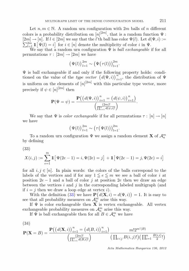
MULTIGRAPH LIMIT OF THE DENSE CONFIGURATION MODEL 211
Let n, m ∈ N. A random urn configuration with 2m balls of n differentcolors is a probability distribution on [n][2m], that is a random function Ψ :[2m] → [n]. If l ∈ [2m] we say that the l’th ball has color Ψ(l). Let d(Ψ, i) :=∑2m
l=1 11[Ψ(l) = i
]for i ∈ [n] denote the multiplicity of color i in Ψ.
We say that a random urn configuration Ψ is ball exchangeable if for allpermutations τ : [2m] → [2m] we have
(Ψ(l)
) 2m
l=1∼ (Ψ
(τ(l)
))2m
l=1.
Ψ is ball exchangeable if and only if the following property holds: condi-tioned on the value of the type vector
(d(Ψ, i)
)n
i=1, the distribution of Ψ
is uniform on the elements of [n][2m] with this particular type vector, moreprecisely if ψ ∈ [n][2m] then
P(Ψ = ψ) =P(
(d(Ψ, i)
)n
i=1=
(d(ψ, i)
)n
i=1)((2m)!
Qni=1 d(ψ,i)!
) .
We say that Ψ is color exchangeable if for all permutations τ : [n] → [n]we have
(Ψ(l)
) 2m
l=1∼ (τ
(Ψ(l)
))2m
l=1.
To a random urn configuration Ψ we assign a random element X of Amn
by defining
X(i, j) :=m∑
e=1
11[Ψ(2e − 1) = i,Ψ(2e) = j
]+ 11
[Ψ(2e − 1) = j,Ψ(2e) = i
](33)
for all i, j ∈ [n]. In plain words: the colors of the balls correspond to thelabels of the vertices and if for any 1 � e � m we see a ball of color i atposition 2e − 1 and a ball of color j at position 2e then we draw an edgebetween the vertices i and j in the corresponding labeled multigraph (andif i = j then we draw a loop edge at vertex i).
With the definition (33) we have P(d(X, i) = d(Ψ, i)
)= 1. It is easy to
see that all probability measures on Amn arise this way.
If Ψ is color exchangeable then X is vertex exchangeable. All vertexexchangeable probability measures on Am
n arise this way.If Ψ is ball exchangeable then for all B ∈ Am
n we have
P(X = B) =P(
(d(X, i)
)n
i=1=
(d(B, i)
)n
i=1)((2m)!
Qni=1 d(B,i)!
)m!2m′(B)
(∏
i<j B(i, j)!)(∏n
i=1B(i,i)
2 !)
(34)
Acta Mathematica Hungarica 136, 2012
212 B. RATH and L. SZAKACS
where m′(B) denotes the number of non-loop edges. The first term in (34)is P(Ψ = ψ) for some ψ that produces B via (33), the second term is thenumber of elements of [n][2m] that produce B via (33).
Recalling the definition of the configuration model (see Section 1) wecan see that if we generate X using (33) from a ball exchangeable urn con-figuration Ψ with a given degree sequence (di)
ni=1 then we in fact uniformly
choose one from the the set of possible matchings of the stubs where the ver-tex i ∈ [n] has di stubs. Thus (34) holds for a random element X of Am
n ifand only if the distribution of X is edge stationary. It is easy to see that alledge-stationary probability distributions on Am
n arise from ball exchangeabledistributions on [n][2m] via (33).
Now we define two different dynamics on random urn configurations:• The Polya urn model: Fix κ ∈ (0,+∞). Let ΨL be a random ele-
ment of [n][L]. Given ΨL we generate a random element of [n][L+1] whichwe denote by ΨL+1 in the following way: let ΨL+1(l) := ΨL(l) for all l ∈ [L]and
∀ i ∈ [n] : P(ΨL+1(L + 1) = i | ΨL
)=
d(ΨL, i) + κ
L + nκ.
• The ball replacement model: Fix κ ∈ (0,+∞). Let ΨT be a randomelement of [n][2m]. Given ΨT we generate a random element of [n][2m] whichwe denote by ΨT+1 in the following way: let ξT denote a uniformly chosenelement of [2m]. For all l ∈ [2m] \ ξT let ΨT+1(l) := ΨT (l) and
(35) ∀ i ∈ [n] : P(ΨT+1(ξT ) = i | ΨT , ξT
)=
d(ΨT , i) + κ
2m + nκ.
It is well-known that if we start with an empty urn Ψ0 and repeatedlyapply the Polya urn scheme to get ΨL for L = 1, 2, . . . , 2m, then the distri-bution of Ψ2m is of the following form:
(36) ∀ ψ ∈ [n][2m] : P(Ψ2m = ψ) =
∏ni=1
∏d(ψ,i)j=1 (κ + j − 1)
∏2mj=1(κn + j − 1)
.
Thus the distribution of Ψ2m is ball and color exchangeable. The PAGκ(n,m)(defined in Section 1) is in fact the random multigraph obtained as the imageof the random urn configuration (36) under the mapping (33).
The ball replacement model is an [n][2m]-valued Markov chain, whichis irreducible and aperiodic with unique stationary distribution (36): if wedelete the ξT ’th ball from Ψ2m, then by ball exchangeability the distributionof the resulting [n][2m−1]-valued random variable is the same as deleting the2m’th ball: Polya-Ψ2m−1. Thus replacing the removed ξT ’th ball with a new
Acta Mathematica Hungarica 136, 2012
MULTIGRAPH LIMIT OF THE DENSE CONFIGURATION MODEL 213
one according to (35) we get a [n][2m]-valued random variable with Polya-Ψ2m distribution again by ball exchangeability.
Now consider the ball replacement Markov chain ΨT , T = 0, 1, . . . withΨ0 being an arbitrary [n][2m]-valued random variable. If we use the mapping(33) to create X(T ) from ΨT , then it is easily seen that the resulting Am
n -valued stochastic process X(T ), T = 0,1, . . . evolves according to the rules ofthe edge reconnecting Markov chain defined in Section 1. Some consequencesof this fact:
• If the distribution of Ψ0 is ball exchangeable then ΨT is also ball ex-changeable for all T , thus if X(0) is edge stationary then so is X(T ) for allT (hence the name “edge stationarity”).
• The distribution (36) is stationary for the ball replacement model, thusthe image of this distribution under the mapping (33) is the unique station-ary distribution of the edge reconnecting model. Lemma 2.1 follows from(36) and (34).
4.1. Limits of edge stationary multigraph sequences. The key re-sult of this subsection is Lemma 4.1 which can be roughly summarized asfollows: in a large dense edge stationary random multigraph the number ofedges connecting the vertices v and w has Poisson distribution with param-eter proportional to d(v)d(w). Given Lemma 4.1 the proof of Theorem 1 isstraightforward and the proof of Theorem 2 reduces to a limit theorem whichstates that the rescaled number of balls with color 1, 2, . . . , k in the Polyaurn model converge in distribution to i.i.d. random variables with Gammadistribution.
Lemma 4.1. Let F : [0,+∞) → [0, 1] denote the cumulative distribu-tion function of a nonnegative random variable Z. Let F −1(u) := min
{x :
F (x) � u}
. Let Z1, Z2, . . . be i.i.d. random variables with Zi ∼ Z ∼ F −1(Ui)(where Ui are uniform on [0, 1]).
If Xn is an An-valued random variable for n = 1, 2, . . . , moreover thedistribution of Xn is vertex exchangeable and edge stationary, and
(37)2m(Xn)
n2
p−→ ρ, n → ∞,
where 0 < ρ < +∞ is positive real parameter, moreover for all k ∈ N we have
(38)(
1n
d(Xn, i))k
i=1
d−→ (Zi)ki=1, n → ∞
Acta Mathematica Hungarica 136, 2012
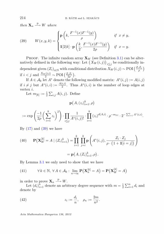
214 B. RATH and L. SZAKACS
then Xnp−→ W where
(39) W (x, y, k) =
⎧⎪⎪⎪⎨
⎪⎪⎪⎩
p(
k,F −1(x)F −1(y)
ρ
)if x = y,
11[2|k] · p(
k
2,F −1(x)F −1(y)
2ρ
)if x = y.
Proof. The infinite random array XW (see Definition 3.1) can be alter-natively defined in the following way: Let
(XW (i, j)
)i�j
be conditionally in-
dependent given (Zi)i∈Nwith conditional distribution XW (i, j) ∼ POI (ZiZj
ρ )if i < j and XW (i,i)
2 ∼ POI (ZiZi
2ρ ).If A ∈ Ak let A∗ denote the following modified matrix: A∗(i, j) := A(i, j)
if i = j but A∗(i, i) := A(i,i)2 . Thus A∗(i, i) is the number of loop edges at
vertex i.Let m[k] := 1
2
∑i,j A(i, j). Define
p(A, (zi)
ki=1, ρ
)
:= exp
(−12ρ
( k∑
i=1
zi
)2)
·∏
i�j
1A∗(i, j)!
·k∏
i=1
(zi)d(A,i) · ρ−m[k] · 2−
Pki=1 A∗(i,i).
By (17) and (39) we have
P(X[k]W = A | (Zi)
ki=1) =
k∏
i=1
k∏
j=i
p
(
A∗(i, j),Zi · Zj
ρ ·(1 + 11[i = j]
)
)
(40)
= p(A, (Zi)
ki=1, ρ
).
By Lemma 3.1 we only need to show that we have
(41) ∀ k ∈ N, ∀ A ∈ Ak : limn→∞
P(X[k]n = A) = P(X[k]
W = A)
in order to prove Xnp−→ W .
Let (di)ni=1 denote an arbitrary degree sequence with m = 1
2
∑ni=1 di and
denote by
(42) zi :=di
n, ρn :=
2mn2
.
Acta Mathematica Hungarica 136, 2012
MULTIGRAPH LIMIT OF THE DENSE CONFIGURATION MODEL 215
Fix ε > 0 and A ∈ Ak. We are going to prove that if
(43) ε � ρn � ε−1, ∀ i ∈ [k] : zi � ε−1
then
P(X[k]
n = A∣∣∣(d(Xn, i)
)k
i=1= (di)
ki=1,
2m(Xn)n2
= ρn
)(44)
= p(A, (zi)
ki=1, ρn
)+ Err (n,A, ε)(45)
with limn→∞ Err (n,A, ε) = 0. We adapt the convention that the value ofErr (n, A, ε) might change from line to line.
First we assume that (44) = (45) holds under the condition (43), anddeduce (41) from it. Define the events Bε
n and Bε by
Bεn :=
{ε � 2m(Xn)
n2� ε−1, ∀ i ∈ [k] :
1n
d(Xn, i) � ε−1
}
Bε :={
ε � ρ � ε−1, ∀ i ∈ [k] : Zi � ε−1}
.
Using the Portmanteau theorem and (37), (38) we obtain the inequalitylim sup
n→∞P(Bε
n) � P(Bε).
|P(X[k]n = A) − P(X[k]
W = A)| (40)= |P(X[k]
n = A) − E(p(A, (Zi)
ki=1, ρ
))|
(46)
�∣∣∣∣∣E
(
p
(
A,
(1n
d(Xn, i))k
i=1
,2m(Xn)
n2
)
;Bn
)
− E(p(A, (Zi)
ki=1, ρ
))
∣∣∣∣∣
(47)
+ Err (ε,A, n) +(1 − P(Bε
n)).(48)
By (37), (38), limn→∞ Err (n,A, ε) = 0 and the fact that p(A, (·)k
i=1, ·)
is abounded continuous function on the domain (43) we obtain
lim supn→∞
(47) � 1 − P(Bε) and lim supn→∞
(48) � 1 − P(Bε).
Now P(Bε) → 1 as ε → 0, from which (41) and the statement of the lemmafollows under the assumption that (43) implies (44) = (45). �
Acta Mathematica Hungarica 136, 2012
216 B. RATH and L. SZAKACS
Proof of (43) =⇒ (44) = (45). We are using random urn configura-tions to generate Xn. Let Ψn denote the ball and color exchangeable [n][2m]-valued random variable with
(d(Ψ, i)
)n
i=1= (di)
ni=1, thus Ψn is uniformly
distributed on the set of urn configurations with this type vector. Xn can begenerated from Ψn via (33). To determine the distribution of X[k]
n we onlyneed to know the positions of the balls of color i ∈ [k]. We paint the rest ofthe balls “grey”. Let
m[k] :=12
∑
i,j
A(i, j), d[k] :=k∑
i=1
di, mg := m − d[k] + m[k].
Thus mg denotes the number of edges of the multigraph spanned by greyvertices.
In order to prove (44) = (45) we first give an explicit formula for (44).The number of grey balls is 2m − d[k]. The number of all urn configurationswith type vector (d1, . . . , dk, 2m − d[k]) is
(49)(2m)!
(∏k
i=1 di!) · (2m − d[k])!
The number of urn configurations with type vector (d1, . . . , dk,2m − d[k])for which X[k]
n = A is
(50)m! · 2m−mg −
Pki=1 A∗(i,i)
(∏
i�j A∗(i, j)!) · (∏k
i=1
(di − d(A, i)
)!) · mg!
.
Thus (44) = (50)(49) . Our aim is to prove (50)
(49) = (45): after dividing both sides
of this equality by∏
i�j1
A∗(i,j)! · 2−P
i A∗(i,i) we only need to prove
m! · (∏k
i=1 di!) · (2m − d[k])! · 2m−mg
∏ki=1
(di − d(A, i)
)! · mg! · (2m)!
(51)
= exp
(−12ρn
( k∑
i=1
zi
)2)
·k∏
i=1
(zi)d(A,i) · ρ
−m[k]n + Err (n,A, ε).(52)
Now we rewrite (51):
(51) =( k∏
i=1
d(A,i)∏
l=1
(di − d(A, i) + l
))
Acta Mathematica Hungarica 136, 2012
MULTIGRAPH LIMIT OF THE DENSE CONFIGURATION MODEL 217
·( m−mg∏
l=1
(mg + l))
· 2m−mg
∏d[k]
l=1 (2m − d[k] + l)
=( m−mg∏
l=1
2mg + 2l2m − d[k] + l
)·∏k
i=1
∏d(A,i)l=1
(di − d(A, i) + l
)
∏m[k]
l=1 (2m − m[k] + l).(53)
We approximate various terms that appear on the right hand side of (53)using our assumptions (43):
m−mg∏
l=1
2mg + 2l2m − d[k] + l
=( d[k]∏
l=1
2m − 2l2m − l
)·(
1 +1n
Err (A, ε))
(54)
m[k]∏
l=1
(2m − m[k] + l) = (2m)m[k] ·(
1 +1n2
Err (A, ε))
(55)
where 0 �∣∣Err (A, ε)
∣∣ < +∞ is independent of n.Let d∗ = min
{di : i ∈ [k], d(A, i) > 0
}. We consider two cases sepa-
rately: If d∗ � n1/2 then using (43) it is easy to see that (53) � Err (A,ε)n−1/2
and also p(A, (zi)
ki=1, ρn
)� Err (A, ε)n−1/2, so (51) = (52) holds when
d∗ � n1/2. If d∗ > n1/2 then we have
(56)k∏
i=1
d(A,i)∏
l=1
(di − d(A, i) + l) =( k∏
i=1
(di)d(A,i)
) (1 +
1√n
Err (A, ε))
.
Putting (54), (55) and (56) together we get
(53) =( d[k]∏
l=1
2m − 2l2m − l
)·∏k
i=1 (di)d(A,i)
(2m)m[k]·(1 + Err (n,A, ε)
)
(42)=
( d[k]∏
l=1
1 − 2ln2ρn
1 − ln2ρn
)·∏k
i=1 (n · zi)d(A,i)
(n2ρn)m[k]·(1 + Err (n,A, ε)
)
(43)= exp
(−12ρn
( k∑
i=1
zi
)2)
·k∏
i=1
(zi)d(A,i) · ρ
−m[k]n + Err (n,A, ε).
This completes the proof of (51) = (52). �
Acta Mathematica Hungarica 136, 2012
218 B. RATH and L. SZAKACS
Proof of Theorem 1. Given Xn for every n ∈ N let us define thevertex exchangeable random adjacency matrix Xn in the following way: letπn denote a uniformly distributed permutation πn : [n] ↪→ [n], independentfrom Xn. Let
(57)(Xn(i, j)
)n
i,j=1:= (Xn
(πn(i), πn(j))
n
i,j=1.
Then Xn is indeed vertex exchangeable, moreover P(t=(F, Xn) = t=(F,Xn)
)
= 1 for every F ∈ M, so Xnp−→ W is equivalent to Xn
p−→ W , which is inturn equivalent to Xn
d−→ XW by Lemma 3.1. By (57) the conditions (11)and (12) are equivalent to the uniform integrability of
(Xn(1, 2)
) ∞n=1
and(Xn(1,1)
) ∞n=1
, respectively, thus we can apply Lemma 3.2(ii) to deduce thatfor all k ∈ N
(58)(
1n
d(Xn, i
))k
i=1
d−→(D(XW , i)
)k
i=1.
Note that by (6), Definition 3.1 and (22) we have that(D(XW , i)
)k
i=1are i.i.d. with probability distribution function FW (z).
Now we are going to prove that 2m(Xn)n2
p−→ ρ(W ). In order to do so wedefine the truncated adjacency matrix Xl
n by X ln(i, j) := min
{Xn(i, j), l
}
and the truncated multigraphon W l which satisfies(XW l(i, j)
) ∞i,j=1
∼ (min{
XW (i, j), l})
∞i,j=1
.
Now we show that if we fix l ∈ N then 2m(Xln)
n2
p−→ ρ(W l). The equationsmarked by (∗) below are true by exchangeability:
limn→∞
E(
1n
n∑
i=1
1n
d(Xln, i)
)(∗)= lim
n→∞E
(1n
d(Xl
n, 1))
(58)= E
(D(XW l , 1)
) (19)= ρ(W l).
limn→∞
D2
(1n
n∑
i=1
1n
d(Xl
n, i))
= limn→∞
1n2
n∑
i,j=1
Cov(
1n
d(Xl
n, i),1n
d(Xl
n, j))
(∗)= lim
n→∞
(1nD2
(1n
d(Xl
n, 1))
+n − 1
nCov
(1n
d(Xl
n, 1),1n
d(Xl
n, 2)))
(58)= 0.
Acta Mathematica Hungarica 136, 2012
MULTIGRAPH LIMIT OF THE DENSE CONFIGURATION MODEL 219
Having established ∀ l : 2m(Xln)
n2
p−→ ρ(W l), the relation 2m(Xn)n2
p−→ ρ(W ) fol-lows from
liml→∞
ρ(W l) = ρ(W ),
∀ ε > 0 : liml→∞
supn∈N
P
(2m(Xn)
n2−
2m(Xl
n
)
n2� ε
)(11), (12)
= 0,
and the ε/3-argument. So conditions (37) and (38) are satisfied, thus we canapply Lemma 4.1 to show that Xn
p−→ W , where W is of the form (13). �
Proof of Theorem 2. The distribution (14) arises from the PolyaΨn
2m urn model (36) with 2m balls and n colors via (33). The distribu-tion (36) is ball and color exchangeable, so Xn is vertex exchangeable andedge stationary. If we want to prove Theorem 2 then by Lemma 4.1 we onlyneed to show that (38) holds for all k ∈ N where (Zi)i∈N
are i.i.d. with den-sity function g(x, κ, κ
ρ ) (see (10)). We may use the method of moments toprove convergence in distribution, since the Gamma distribution is uniquelydetermined by its moments. Thus we need to show that if ν1, . . . , νk ∈ N
then
limn→∞
E( k∏
i=1
(1n
d(Ψn2m(n), i)
)νi)
= E( k∏
i=1
Zνi
i
)
=k∏
i=1
(ρ
κ
)νi
·νi∏
j=1
(κ + j − 1).
Fix k and νi, i ∈ [k]. Let ν =∑k
i=1 νi and denote by ψ a particular elementof [k][ν] with type vector (ν1, . . . , νk). By the construction of the Polya-Ψn
2mdistribution we have
P(
∀ l ∈ [ν] : Ψn2m(l) = ψ(l)
)=
∏ki=1
∏νi
j=1(κ + j − 1)∏ν
j=1(κn + j − 1)= O(n−ν)
Denote ν :={
(i, j) : i ∈ [k], j ∈ [νi]}
. The number of functions f : ν → [2m]with
∣∣ R(f)∣∣ = N is O(
(2m(n)
)N) = O(n2N ) if 1 � N � ν.
limn→∞
E
(k∏
i=1
(1n
d(Ψn2m(n), i)
)νi
)
Acta Mathematica Hungarica 136, 2012
220 B. RATH and L. SZAKACS
= limn→∞
1nν
∑
f : ν→[2m]
P(∀ (i, j) ∈ ν : Ψn2m(n)
(f(i, j)
)= i)
= limn→∞
1nν
∑
f : ν↪→[2m]
P(∀ (i, j) ∈ ν : Ψn2m(n)
(f(i, j)
)= i)
+ limn→∞
1nν
ν−1∑
N=1
O(n2N
)O
(n−N
)
(∗)= lim
n→∞
∏νk=1
(2m(n) − k + 1
)
nνP
(∀ l ∈ [ν] : Ψn
2m(l) = ψ(l))
(37)=
k∏
i=1
(ρ
κ
)νi
·νi∏
j=1
(κ + j − 1).
The equation (∗) holds true by ball exchangeability. �
References
[1] D. J. Aldous, Representations for partially exchangeable arrays of random variables,J. Multivar. Anal., 11 (1981), 581–598.
[2] D. J. Aldous, More uses of exchangeability: representations of complex random struc-tures, arXiv: 0909.4339v2, to appear in Probability and Mathematical Genetics:Papers in Honour of Sir John Kingman, Cambridge University Press (2010).
[3] P. Billingsley, Convergence of Probability Measures, 2nd ed., John Wiley & Sons, Inc.(New York, 1999).
[4] C. Borgs, J. Chayes and L. Lovasz, Moments of two-variable functions and the unique-ness of graph limits, Geom. Funct. Anal., 19 (2010), 1597–1619.
[5] C. Borgs, J. Chayes, L. Lovasz, V. Sos and K. Vesztergombi, Limits of randomlygrown graph sequences, Eur. J. Combin., 32 (2011), 985–999.
[6] S. Chatterjee, P. Diaconis and A. Sly, Random graphs with a given degree sequence,Ann. Appl. Probab., 21 (2011), 1400–1435.
[7] P. Diaconis and S. Janson, Graph limits and exchangeable random graphs, Rend. Mat.Appl., 28 (2008), 33–61.
[8] I. Kolossvary and B. Rath, Multigraph limits and exchangeability, Acta Math. Hun-gar., 130 (2011), 1–34.
[9] L. Lovasz, Very large graphs, in: Current Developments in Mathematics 2008, Inter-national Press (Somerville, MA, 2009), pp. 67–128.
[10] L. Lovasz and B. Szegedy, Limits of dense graph sequences, J. Combin. Theory Ser. B,96 (2006), 933–957.
[11] L. Lovasz and B. Szegedy, Random graphons and weak positivstellensatz for graphs,arXiv: 0902.1327v1, to appear in Journal of Graph Theory (2011).
[12] L. Lovasz and B. Szegedy, Limits of compact decorated graphs, arXiv: 1010.5155v1(2010).
MULTIGRAPH LIMIT OF THE DENSE CONFIGURATION MODEL 221
[13] B. Rath, Time evolution of dense multigraph limits under edge-conservative preferen-tial attachment dynamics (accepted for publication in Random Structures andAlgorithms), arXiv: 0912.3904v3 (2010).
[14] M. Reed and B. Simon, Methods of Modern Mathematical Physics, vol. 1: FunctionalAnalysis, Gulf Professional Publishing (1980).
[15] D. Williams, Probability with Martingales, Cambridge University Press (Cambridge,1991).