Page 1
ORIGINAL PAPER
Multilayer network model for analysis and managementof change propagation
Michael C. Pasqual • Olivier L. de Weck
Received: 29 September 2010 / Revised: 19 May 2011 / Accepted: 22 November 2011 / Published online: 7 December 2011
� Springer-Verlag London Limited 2011
Abstract A pervasive problem for engineering change
management is the phenomenon of change propagation by
which a change to one part or element of a design requires
additional changes throughout the product. This paper
introduces a multilayer network model integrating three
coupled layers, or domains, of product development that
contribute to change propagation: namely, the product
layer, change layer, and social layer. The model constitutes
a holistic, data-driven approach to the analysis and man-
agement of change propagation. A baseline repository of
tools and metrics is developed for the analysis and man-
agement of change propagation using the model. The
repository includes a few novel tools and metrics, most
notably the Engineer Change Propagation Index (Engineer-
CPI) and Propagation Directness (PD), as well as others
already existing in the literature. As such, the multilayer
network model unifies previous research on change prop-
agation in a comprehensive paradigm. A case study of a
large technical program, which managed over 41,000
change requests in 8 years, is employed to demonstrate the
model’s practical utility. Most significantly, the case study
explores the program’s social layer and discovers a corre-
spondence between the propagation effects of an engi-
neer’s work and factors such as his/her organizational role
and the context of his/her assignments. The study also
reveals that parent–child propagation often spanned two or
more product interfaces, thus confirming the counterintui-
tive possibility of indirect propagation between nonadja-
cent product components or subsystems. Finally, the study
finds that most changes did not lead to any propagation.
Propagation that did occur always stopped after five, and
rarely more than four, generations of descendants.
Keywords Engineering change management �Product development � Change propagation �Multilayer network model � Multiple domains
Abbreviations
CAI Change Acceptance Index
CPI Change Propagation Index
CPM Change Prediction Method
CR Change request
CRI Change Reflection Index
DMM Domain Mapping Matrix
DSM Design Structure Matrix
ECM Engineering change management
ESM Engineering Systems Matrix
IPT Integrated program team
PAR Proposal Acceptance Rate
PD Propagation Directness
PDSM Propagation Design Structure Matrix
SAP System Adjustable Parameter
1 Introduction
The design of a complex product is rarely, if ever,
straightforward or permanent. In fact, an organization is
practically bound to make design changes throughout the
conception, development, implementation, and operation
Present Address:M. C. Pasqual (&)
MIT Lincoln Laboratory, Lexington, MA, USA
e-mail: [email protected]
O. L. de Weck
Engineering Systems Division, Massachusetts Institute
of Technology, E40-261,77 Massachusetts Ave.,
Cambridge, MA 02139, USA
e-mail: [email protected]
123
Res Eng Design (2012) 23:305–328
DOI 10.1007/s00163-011-0125-6
Page 2
of almost any product (Nichols 1990; Pikosz and Malmqvist
1998). The process of engineering change management
must balance the costs, benefits, and risks of implementing
design changes, in light of their implications for schedule,
budget, and product quality.
A pervasive problem for engineering change management
is the phenomenon of change propagation, by which a
change to one part or element of a design requires additional
changes throughout the product. Change propagation sig-
nificantly contributes to the time, money, and resources
required for evaluating and implementing changes (Clarkson
et al. 2004; Terwiesch and Loch 1999).
The topic of change propagation has received consid-
erable research attention over the last decade. The high-
lights of the literature include qualitative and quantitative
efforts to characterize, predict, control, and prevent change
propagation. These efforts have primarily drawn on net-
work-based analyses by modeling products and change
processes as networks of nodes and edges.
1.1 Research contribution
Building on these contributions, this paper introduces a
multilayer network model integrating three coupled layers,
or domains, of product development that contribute to
change propagation: namely the product layer, change
layer, and social layer. To the authors’ knowledge, no
previous research on change propagation has, at least
explicitly, taken a multilayer network approach. The model
proposed here draws on multilayer (or multi-domain) net-
work approaches already taken in broader research on
product development and project management.
Using a Venn diagram, Fig. 1 summarizes the research
landscape associated with this research. This paper, labeled
‘‘current research,’’ addresses the gap at the intersection of
research on change propagation and multilayer network
analysis.
1.2 Research framework
Motivated by this gap, this paper investigates the following
research questions:
• What insights can be gained from a multilayer network
model of change propagation?
• What are potential tools and metrics for analyzing the
model?
• How can the model contribute to the prevention,
prediction, and control of change propagation?
The overarching hypothesis is that a multilayer network
model provides a holistic, data-driven framework for the
analysis and management of change propagation. The
multilayer perspective urges an organization to consider
the influence of all three layers (product, change, and
social) when trying to prevent, predict, and control change
propagation. A baseline repository of tools and metrics is
developed for use with the model. The repository includes
a few novel tools and metrics, in addition to others already
existing in the literature. As such, the model unifies pre-
vious research on change propagation in a comprehensive
paradigm.
To demonstrate the model’s practical utility, this paper
discusses a case study of a large technical program that
managed over 41,000 change requests in 8 years. Giffin
Fig. 1 Relevant research
landscape
306 Res Eng Design (2012) 23:305–328
123
Page 3
(2007) and Giffin et al. (2009) performed earlier studies of
the same program. The case study in this paper uses an
array of multilayer network tools and metrics to address
two important topics. The first topic revolves around the
social layer’s effects on change propagation; the investi-
gation reveals interesting aspects of an engineer’s perfor-
mance in the implementation and proposal of changes. The
second topic focuses on the general characterization of
change propagation. The primary issue discussed here is
the counterintuitive phenomenon of indirect propagation,
by which propagation occurs between nonadjacent product
components. Additionally, the study finds that most chan-
ges did not lead to any propagation in the program’s system
design. Propagation that did occur always stopped after
five, and rarely more than four, generations of descendants.
The remainder of this paper is structured as follows.
Section 2 presents relevant background material in the
form of a brief literature review. Section 3 introduces the
multilayer network model of change propagation. A simple
hypothetical example is used to illustrate the model. Sec-
tion 4 develops a baseline repository of tools and metrics
for use with the model. Section 5 conducts a case study to
demonstrate the model’s practical utility. Section 6 pro-
vides a summary of the research findings and recommen-
dations for future work.
2 Background
Engineering change management (ECM) is the branch of
configuration management (N.A.S.A. 2007) concerned
with the identification, evaluation, implementation, and
auditing of changes to the design of a product or system
(Huang and Mak 1999). ECM is a critical process as
changes are inevitable throughout product development
(Nichols 1990; Pikosz and Malmqvist 1998). While chan-
ges theoretically present opportunities for an organization
to improve its products, satisfy its customers, and stay
competitive in its market (Wright 1997), the ECM process
can ultimately consume considerable time, money, and
resources (Terwiesch and Loch 1999).
2.1 Change propagation
Among the reasons why changes can be so abundant and
costly is the occurrence of change propagation. Change
propagation can be defined as the ‘‘process by which a
change to one part or element of an existing system [or
product] configuration or design results in one or more
additional changes to the system, when those changes would
not have otherwise been required’’ (Giffin et al. 2009). In
other words, change propagation occurs when making a
single change ultimately requires the implementation of
multiple changes in order to achieve the objective of the
intended redesign.
For clarity,1 this research has adopted the term parent–
child propagation to refer to the act of one change (the
parent) yielding an immediate descendant change (the
child). Figure 2 shows a single change that yields four
generations of descendants through recursive parent–child
propagation. Propagation over this many generations has
been reported in the literature (Clarkson et al. 2004) and
will be reaffirmed in Sect. 5’s case study.
Change propagation occurs because of the interdepen-
dencies among the components and subsystems of modern
products and systems (Earl et al. 2005; Suh and de Weck
2007). Eckert et al. (2004) explain that different parts of a
product exhibit different propagation behavior. Compo-
nents that are absorbers tend to internalize changes without
causing many changes to other components. By contrast,
multipliers give rise to more changes than they absorb.
Meanwhile, carriers absorb and cause a roughly equal
number of changes. Finally, constants do not contribute to
any propagation; they are only affected by isolated changes
or do not change at all.
Because of its significant implications for engineering
change management, product development, and business
strategy, the topic of change propagation has received
considerable research attention over the last decade. Efforts
to quantitatively characterize, predict, control, and prevent
change propagation, though limited, have primarily drawn
on network-based models and analyses.
2.2 Network-based analysis of change propagation
Change propagation research has quite naturally turned to
network-based models and analyses rooted in graph theory.
After all, many aspects of product development and project
Fig. 2 In this change network, unidirectional and bidirectionalarrows indicate parent–child and sibling–sibling relationship between
changes, respectively
1 Otherwise it can be confusing whether the term ‘‘propagation’’
refers to a single instance or repeated instances of parent–child
propagation.
Res Eng Design (2012) 23:305–328 307
123
Page 4
management (e.g., products, processes, and organizations)
are readily modeled as networks.
At the heart of most previous research on change prop-
agation is the popular tool known as the Design Structure
Matrix (DSM) (Steward 1981; Eppinger et al. 1994).
A DSM is an adjacency matrix representation of a directed
network. The DSM can be used to represent a product
consisting of interconnected components, a process con-
sisting of tasks, or an organization consisting of people. The
DSM concept has proven extremely influential in the
quantitative investigation of change propagation. For
instance, Clarkson et al.’s (2004) Change Prediction Model
(CPM) uses the DSM representation of a product to trace
potential propagation paths among its interconnected
components. Similarly, Giffin et al. (2009) extend the DSM
concept to create the Component Propagation DSM
(Component-PDSM) to identify instances of change prop-
agation from one component to another.2 In kind, one can
calculate the Change Propagation Index (CPI), which
quantifies a component’s propagation behavior by com-
paring the numbers of changes that propagate in and out of
that component (Suh and de Weck 2007; Giffin et al. 2009).
Despite the progress of change propagation research to
date, a new approach, specifically a multilayer network
one, may be beneficial to the field. Broader literature on
product development and project management has
emphasized the existence of multiple network layers, or
domains, in an engineering endeavor, including product,
process, and social layers. To date, change propagation
research has not, at least explicitly, taken a multilayer
network approach. To be fair, tools and metrics like the
Component-PDSM and CPI are arguably double-layer
approaches, since they do consider both the product layer
and change (i.e., process) layer. Still, other contributions
like the DSM and CPM rely on a single-layer model of the
design and change layers, respectively. Moreover, change
propagation research surprisingly has yet to investigate the
social layer in a substantially quantitative way. Neverthe-
less, the literature has at least qualitatively stressed the
significance of teamwork, individual skills, and system
awareness in the ECM process (Huang and Mak 1999;
Jarratt et al. 2006).
2.3 Multilayer network approaches
Multilayer, or multi-domain, network approaches are pre-
valent in the literature on product development and project
management. The premise of these approaches is that the
success of product development depends significantly on
the interactions within and among the various domains
(e.g., product, process, social) of the development effort.
For example, Danilovic and Browning (2007) propose a
variation of the DSM called the Domain Mapping Matrix
(DMM), which captures the dependencies between any two
domains of product development, including the product
design, development process, and development organiza-
tion. Bartolomei’s (2007) Engineering Systems Matrix
(ESM) augments the DSM even further. The ESM incor-
porates several domains (e.g., technical, functional, pro-
cess, social, and environmental) into a single adjacency
matrix representing edges within and between nodes in
each domain. By grouping the nodes by domain, the ESM
essentially contains DSMs on the diagonal and DMMs in
the upper and lower triangles. Finally, Eppinger (2001)
advocates a multi-domain model most analogous to the one
proposed in this paper. He specifically investigates whether
interactions within the product, process, and organization
domains tend to follow a common, predictable pattern
(Morelli et al. 1995; Sosa et al. 2000, 2007; Eppinger
2001).
Thus, the stage is set for further analysis of product
development using a multilayer network approach. This
paper extends the approach to the analysis and manage-
ment of change propagation.
3 Multilayer network model of change propagation
This section introduces a multilayer network model of
change propagation. The model is composed of three layers
that contribute to change propagation: the product layer,
change layer, and social layer. As illustrated in Fig. 3, the
multilayer network model provides an intuitive and
insightful representation of change propagation and the
overall engineering change management process. That is,
engineers in the social layer work on changes in the
change layer that affect components in the product layer.
The multilayer network model captures the interactions
within and across the product layer, change layer, and
social layer.
3.1 Elements of the model
Each layer of the multilayer network model consists of a
distinct, directed network composed of nodes connected by
intra-layer edges.
3.1.1 Product layer
The product layer is a network representation of the
product or system being designed. The nodes of the
2 Giffin et al. (2009) actually name this tool the Change DSM or
DDSM, but this paper substitutes the word ‘‘propagation’’ for
‘‘change’’ to help distinguish it from a DSM used to represent a
change network.
308 Res Eng Design (2012) 23:305–328
123
Page 5
network represent hardware components, software com-
ponents, and associated documentation (e.g., requirements,
specifications, and drawings). The (intra-layer) edges of the
network represent technical interfaces among the compo-
nents (or subsystems). The interfaces can be physical
connections (e.g., by bolts or welding) or channels for the
flow of energy (e.g., electrical power and heat), mass (e.g.,
fuel), and information (e.g., software inputs/outputs and
control signals such as actuator commands) (Suh and de
Weck 2007). If a technical interface has direction (e.g., in
the case of a flow channel), the edges can be directed. An
edge might also identify a functional dependency that
relates design variables to a desired performance level
(e.g., in an optical system, image resolution is a function of
aperture diameter).
3.1.2 Change layer
The change (or process) layer is a network representation
of change propagation. The nodes of the network repre-
sent individual changes or change requests (CRs). The
(intra-layer) edges of the network represent propagation
relationships among the changes. As in Fig. 2 and Giffin
et al. (2009), directed edges can identify parent–child
relationships, while bidirectional edges can identify sib-
ling relationships between children of the same parent or
two changes related in a significant way.
3.1.3 Social layer
The social layer is a network representation of the orga-
nization. The nodes of the network represent people, e.g.,
teams, sub-teams, or individual engineers or employees.
The (intra-layer) edges of the network represent various
relationships among individuals and groups. For example,
the edges might correspond to theoretical or actual com-
munication links (Morelli et al. 1995). The edges might
also reflect an organization’s hierarchical structure or chain
of command.
One might also consider edge strength when identifying
intra-layer edges, particularly in the product layer and
social layer. After all, a strong connection between nodes
might exhibit different behavior than a weaker connection.
For example, Sosa et al. (2000) use a five-point scale to
denote the criticality of interactions among product com-
ponents, according to whether the interaction is required
(?2), desired (?1), indifferent (0), undesired (-1), or
detrimental (-2) to the functionality of the product. Their
case study of the development of a commercial aircraft
engine found that strong technical interfaces in the engine,
compared to weaker ones, more often elicited communi-
cation in the corresponding organization domain. Conse-
quently, it might be useful to incorporate edge strength into
the multilayer network model, if an objective and consis-
tent quantification scheme is employed.
3.1.4 Inter-layer edges
The other half of the multilayer network model consists of
the inter-layer edges that essentially link the three layers
together. Unlike the intra-layer edges, the inter-layer edges
are nominally undirected (or bidirectional). The inter-layer
edges represent the critical relationships between the layers
of the model:
• Social-to-change edges relate the social layer to the
change layer, depending on which engineers work on
(e.g., propose, evaluate, approve, or implement) each
change. If engineer m works on change n, then an inter-
layer edge would connect node m in the social layer and
node n in the change layer.
• Change-to-product edges relate the change layer to the
product layer, depending on which component is
affected by each change. If change n involves a
Fig. 3 Multilayer network model
Res Eng Design (2012) 23:305–328 309
123
Page 6
redesign of component k, then an inter-layer edge
would connect node n in the change layer and node k in
the product layer.
• Product-to-social edges relate the product layer to the
social layer, depending on which engineers are in
charge of designing, redesigning, or sourcing each
component. If engineer m is assigned to component k,
then an inter-layer edge would connect node m in the
social layer and node k in the product layer. Figure 3
does not illustrate the product-to-social edges, but they
could be included, if desired.
3.2 Data requirements
The construction of a multilayer network model requires
detailed information about the product development effort
under investigation. Table 1 summarizes the type of data
needed to construct each model element described in Sect.
3.1, as well as potential sources of such data within the
documentation conventionally maintained by an organiza-
tion during product development.
As shown in Table 1, the multilayer network model is a
data-driven approach to the analysis and management of
change propagation. Of course, different amounts and types
of data are available at different stages of product devel-
opment. As such, the multilayer network model has dif-
ferent utility at different stages, i.e., before, during, and
after product development. Before product development,
complete data on the nodes and edges will likely not exist,
because all the components, change requests, engineers, and
their relationships will not have manifested themselves yet.
However, some insight may be gained by modeling analo-
gous development efforts from the past, especially since
most products are adaptations of predecessor products
(Giffin et al. 2009). Later, during product development, data
can be progressively collected through configuration man-
agement, which allows the construction of a multilayer
network model with whatever fidelity and completeness
that the organization wishes. Analysis of the model during
product development can be used to guide change impact
analysis, organization structuring, design strategy, and
human resource management. Finally, after product
development, analysis of the multilayer network becomes a
lessons-learned effort. At this stage, an organization can use
all the data collected over the course of product develop-
ment to assess its performance in retrospect. Moreover, the
data then become useful for academic research to further
investigate industry’s experience with change propagation.
3.3 Hypothetical application
A hypothetical application should illustrate how to con-
struct a multilayer network model for a given product
development effort.
Suppose three engineers, John, Susan, and David, are
designing a Sallen–Key low-pass filter (Fig. 4) using two
resistors (R1 and R2), two capacitors (C1 and C2), and a unity-
gain amplifier. The amplifier has already been purchased.
John is in charge of choosing the resistors, Susan is in charge
of choosing the capacitors, and David is in charge of setting
performance requirements, i.e., cutoff frequency (xc) and
quality factor (Q). The resistors (in ohms) and capacitors (in
farads) determine the low-pass filter’s performance (xc in Hz
and Q unitless) according to Eqs. 1 and 2.
xc ¼1
2pffiffiffiffiffiffiffiffiffiffiffiffiffiffiffiffiffiffiffiffi
R1R2C1C2
p ð1Þ
Q ¼ffiffiffiffiffiffiffiffiffiffiffiffiffiffiffiffiffiffiffiffi
R1R2C1C2
p
C2ðR1 þ R2Þð2Þ
Suppose the low-pass filter has been designed to have a
baseline cutoff frequency of xc = 10 kHz, and quality
factor Q = 0.5 (i.e., critically damped), per David’s initial
performance requirements. However, some changes
become necessary. David decides that the cutoff frequency
Table 1 Data requirements for the multilayer network model
Model element Data required Potential source
Nodes Product layer Components Design documents
Change layer Change requests Configuration management records
Social layer Engineers Staffing records
Intra-layer edges Product layer Interfaces among components Interface control documents
Change layer Propagation relationships among change requests Configuration management records
Social layer Communication links among engineers Meeting agendas, minutes, notes, and other records
Inter-layer edges Social-to-change Engineer who worked on each change Configuration management records
Change-to-
product
Component affected by each change Configuration management records
Product-to-social Engineer in charge of each component Staffing records
310 Res Eng Design (2012) 23:305–328
123
Page 7
should be 5 kHz instead of 10 kHz (change #1), but that
the quality factor should remain at Q = 0.5. To facilitate
this requirements change, the team initially plans for John
to change R1 (change #2), but that change is rejected
because the resistors have already been ordered. Conse-
quently, Susan must reselect the capacitors. Susan realizes
that she cannot simply change one of the capacitors to
accomplish the task of reducing xc while maintaining the
same Q. In effect, the change to one capacitor will prop-
agate, causing the other capacitor to change as well. Susan
ultimately decides to double the original capacitances of C1
(change #3) and C2 (change #4) to reduce xc by a factor of
two (10–5 kHz) while maintaining Q = 0.5.
Figure 5 shows the multilayer network model corre-
sponding to this hypothetical application. The model cap-
tures the major details of the change activity that occurred.
The social layer contains nodes for John, Susan, and David,
with edges representing their communication links. The
change layer contains nodes for changes #1–4 with edges
representing propagation relationships. The edges indicate
that change #1 had two children: change #2 (rejected) and
change #3 (accepted), which also had a child in change #4.
The product layer contains nodes for requirements and
electrical components, with edges representing technical
constraints. All the nodes in the product layer are con-
nected to one another because xc, Q, R1, R2, C1, and C2 all
depend on one another through Eqs. 1 and 2. The inter-
layer edges in Fig. 5 complete the story. The social-to-
change edges represent how David, John, and Susan
worked on changes #1, #2, and #3–4, respectively. The
change-to-product edges represent how change #1, #2, #3,
and #4 affected xc, R1, C1, and C2, respectively. For visual
ease, Fig. 5 does not show any product-to-social edges.
However, if drawn, these edges would represent how John,
Susan, and David were in charge of R1 and R2, C1 and C2,
and xc and Q, respectively.
4 Multilayer network tools and metrics
This section presents a baseline repository of tools and
metrics applicable to the multilayer network model. The
model creates a framework for an array of potential tools
and metrics for analyzing and managing change propaga-
tion. Tools here refer to methods for analyzing or
visualizing the nodes and edges of the model, while metrics
refer to quantitative or quantitative measures for charac-
terizing them. Any use of the multilayer network model
will focus on one layer alone or multiple layers simulta-
neously. Consequently, it is useful to consider any tool or
metric as being single layer, double layer, or triple layer in
origin, depending on the number of layers involved in the
analysis.
4.1 Baseline repository
Table 2 summarizes a baseline repository of tools and
metric by categorizing each item according to the specific
layer or layers it targets. The displayed matrix has a row
and column for each layer of the model. As such, the items
located along the diagonal are single-layer tools and met-
rics for the corresponding individual layer. The items in the
upper-right triangle are double-layer tools and metrics for
the corresponding pairs of layers. Finally, the items in the
lower left triangle are triple-layer tools and metrics for all
three layers at once.
As denoted by references, the repository in Table 2
contains many tools and metrics that have already been
proposed and utilized in the literature on change propaga-
tion, product development, and project management.
Although past researchers did not always explicitly classify
their work in a multilayer context, their contributions are
easily incorporated into the multilayer network model.
Consequently, the multilayer network model serves as a
comprehensive paradigm that unifies past research in a
common framework.
Table 2 also contains a few new tools and metrics
(marked with a ‘‘*’’) that are being proposed for the first
Fig. 4 Sallen–Key low-pass filter to be designed
Fig. 5 Multilayer network model of the low-pass filter example
Res Eng Design (2012) 23:305–328 311
123
Page 8
time in this paper. Among these are the Engineer Propa-
gation DSM (a double-layer tool) and the Engineer Change
Propagation Index (a double-layer metric), which aim to
quantitatively analyze the social layer’s influence on
change propagation. Another new metric in the repository
is Propagation Directness (a double-layer metric) that
counts the number of interfaces spanned by an instance of
parent–child propagation.
4.2 Data requirements for tools and metrics
As discussed in Sect. 3.2, the construction of a multilayer
network model requires data collection and mining.
Table 3 specifies types of data (i.e., elements of the model)
needed to exercise any of the multilayer network tools and
metrics in practice. Such data mining can occur after
completion or, better yet, during product development. The
displayed matrix has a row for each tool or metric and a
column for each type of intra-layer and inter-layer edge.
Check marks (4) denote which edge data would be
required for each tool and metric. For example, to construct
a DSM for a given layer, an organization would need to
know the intra-ledges for that layer. To construct a Com-
ponent-PDSM, an organization would need the intra-layer
edges of the change layer (i.e., propagation relationships)
and the change-to-product inter-layer edges (i.e., which
changes affect which components). Intuitively, single-layer
tools and metrics only require intra-layer edges. By con-
trast, the double-layer and triple-layer tools all tap into the
inter-layer edges as well, because they focus on multiple
layers simultaneously.
The following subsections develop the baseline reposi-
tory of tools and metrics, both old and new. Sections 4.3,
4.4, and 4.5 review the single-layer, double-layer, and tri-
ple-layer tools and metrics, respectively, which already
exist in the literature. Section 4.6 discusses the additional
tools and metrics that are being proposed for the first time
in this paper. Each tool and metric, old and new, is criti-
cally evaluated in terms of its implications for the analysis
and management of change propagation in context of the
multilayer network model.
4.3 Single-layer tools and metrics
Single-layer tools and metrics focus on one layer of the
multilayer network model at a time. These tools and metrics
highlight intra-layer characteristics of great significance for
engineering change management. The single-layer metrics
(graph properties and node attributes), in particular, have
been employed in the change propagation literature, but
without any formal development. This discussion hopes to
officially establish their utility for future research.
Table 2 Baseline repository of tools and metrics for the multilayer network model
Product Change Social
Pro
duct
Tools••
••
••
Design Structure Matrix (1)Change Prediction Model (2)
MetricsGraph properties (3)Node attributes, e.g., component
class (5)
ToolsDomain Mapping Matrix (4)Component Propagation DSM (5)Change Prop. Frequency Matrix (5)
MetricsComponent Change Propagation Index (5, 6)Change Acceptance/Reflectance Rate (5)Propagation Directness*
ToolsDomain Mapping Matrix (4)Alignment Matrix (7)
Cha
nge
ToolsDesign Structure Matrix (1)Change motifs (5)
MetricsGraph properties (3)Node Attributes, e.g., approval status (5),magnitude (5)
ToolsDomain Mapping Matrix (4)Engineer Propagation DSM*
MetricsEngineer Change Propagation Index*Proposal Acceptance Rate (8)
Soci
al
ToolsEngineering System Matrix (9)
MetricsGraph properties (3)
ToolsDesign Structure Matrix (1)
MetricsGraph properties (3)Node attributes, e.g., organizationalrole*
(1) Steward 1981(2) Clarkson et al. 2004(3) Newman 2003(4) Danilovic and Browning 2007(5) Giffin et al. 2009
(6) Suh and de Weck 2007(7) Sosa et al. 2007(8) Giffin 2007(9) Bartolomei 2007* Proposed first in this paper
Single-layer Double-layer Triple-layer
•
•••
••
••
••
••
••
•
••
•
•
312 Res Eng Design (2012) 23:305–328
123
Page 9
4.3.1 Design Structure Matrix (DSM)
The primary single-layer tool from previous research is the
DSM, which, as mentioned in Sect. 2.2, is a convenient
matrix representation of a network (Steward 1981; Eppinger
et al. 1994). As illustrated in Fig. 6, a DSM is a square
matrix in which element (m, n) indicates whether a directed
edge connects node n to node m.
One can create a separate DSM for each layer of the
multilayer network model, i.e., a Product DSM, Change
DSM, and Social DSM. Clustering algorithms (Browning
2001) exist to manipulate the rows and columns of a DSM
to help identify groups (or clusters) of tightly coupled
nodes, e.g., subsystems in the product layer, families of
changes in the change layer, and teams or communication
structures in the social layer. The DSM has significant
implications for engineering change management. An
organization can exploit each layer’s DSM to inform better
engineering and managerial decision, thus minimizing
unnecessary future changes and stemming change propa-
gation. For example, the Product DSM can guide design
architecture decisions in anticipation of the challenges of
testing, building, integrating, and evolving a product (e.g.,
automobiles, Suh and de Weck 2007). Likewise, based
on the Social DSM, a project manager might organize and
co-locate teams to facilitate better communication. Such
strategies are vital to engineering change management, as
Eckert et al. (2004) suggest that insufficient communica-
tion is a primary cause of redesigns throughout product
development.
4.3.2 Change prediction model (CPM)
As mentioned in Sect. 2, CPM is a single-layer tool
developed for predicting the occurrence of change propa-
gation. The tool focuses specifically on the product layer.
CPM uses the Product DSM to identify potential propa-
gation paths between components, under the assumption
that changes propagate along the technical interfaces of a
product. The final product of the tool is a risk matrix
Table 3 Edge data required for multilayer network tools and metrics
Intra-layer edges Inter-layer edges
Product layer
(technical
interfaces)
Change layer
(propagation
relationships)
Social layer
(comm.
links)
Social-to-
change
Change-to-
product
Product-to-
social
Single layer Tools DSM (for each layer) 4 4 4
CPM 4
Change motif 4
Metrics Graph properties (for each layer) 4 4 4
Double
layer
Tools DMM (for each pair of layers) 4 4 4
Component-PDSM 4 4
CPFM 4 4
Product DSM/component-
PDSM overlay
4 4 4
Alignment matrix 4 4 4
Engineer-PDSM 4 4
Metrics Propagation Directness 4 4 4
Component-CPI 4 4
CAI/CRI 4
Engineer-CPI 4 4
PAR 4
Triple layer Tools ESM 4 4 4 4 4 4
Metrics Graph properties 4 4 4 4 4 4
Fig. 6 The DSM succinctly shows where edges exist in a network
Res Eng Design (2012) 23:305–328 313
123
Page 10
indicating the likelihood and impact of propagation
between each and every component in the product
(Clarkson et al. 2004). Another element of the CPM tool is
a set of visualization techniques for viewing potential
propagation paths (Keller et al. 2005).
4.3.3 Change motifs
Giffin et al.’s (2009) change motif analysis is another sin-
gle-layer tool that focuses on the change layer alone. The
premise here is that change networks can be decomposed
into motifs, or building blocks, each with distinct patterns
of changes and propagation relationships. Motif distribu-
tions reveal what types of propagation patterns are domi-
nant in a product.
4.3.4 Graph properties
Several single-layer metrics already exist in the literature
as well. For starters, graph theory (Diestel 2005) provides a
number of properties generally applicable to any layer of
the multilayer network model. For example, the clustering
coefficient is a graph property that measures how much a
network’s nodes tend to cluster together (Newman 2003).
In the product layer, the clustering coefficient roughly
relates to a product’s modularity. Integrative products,
which have relatively high clustering coefficients, may be
more susceptible to change propagation, since their com-
ponents are more interdependent. Another potentially
useful graph property is centrality, which is a gauge of the
importance of a node in a network. One measure of a
node’s centrality is its degree or the number of edges
incident upon it (Newman 2003). In the product layer, a
component’s centrality may reflect its potential propaga-
tion behavior. Namely, components with higher centrality
might be more involved in change propagation, as parents
or children.
4.3.5 Node attributes
Node attributes constitute another set of single-layer met-
rics. Node attributes refer to qualitative or quantitative
measures of a node, other than nodal graph properties. The
attributes of a node might influence its contributions to
change phenomena.
Nodes attributes in the product layer describe the
product components. For example, one node attribute is
component class, i.e., whether a component is hardware,
software, or documentation. Different component classes
might exhibit different change propagation behavior. In
the program from Sect. 5’s case study, the requirements
document was naturally a strong multiplier, because this
component essentially recorded changes to system
requirements, which (almost) always led to redesigns
among the various technical parts of the system. By con-
trast, certain software algorithms behaved as constants,
because altering them was cost and time prohibitive.
Changes (i.e., nodes) in the change layer might be
described by nodes attributes such as magnitude (in terms
of time and resources consumed) and approval status (i.e.,
whether the change is accepted, rejected, or pending).
Giffin et al. (2009) found that high-magnitude changes
were more likely to be approved than low-magnitude ones
because many of the low-magnitude change requests were
deemed to be nonessential. Others attributes in the change
layer include process time and cost.
Finally, node attributes in the social layer describe
individual engineers (or teams). For instance, engineers
have various organizational roles (e.g., specialists, team
lead, systems engineer, or manager), which will likely
impact his or her responsibilities in the engineering change
management process. Section 5’s case study will quanti-
tatively elaborate on this relationship further.
4.4 Double-layer tools and metrics
Double-layer tools and metrics focus on two-layers
simultaneously by taking into account the inter-layer edges
between them.
4.4.1 Domain Mapping Matrix (DMM)
The first notable double-layer tool is Danilovic and
Browning’s (2007) DMM. As introduced in Sect. 2, the
DMM is a matrix representation of the dependencies
between two domains. In the language of this paper, ele-
ment (m, n) of the DMM indicates whether an inter-layer
edge exists between node m in the former layer and node
n in the latter. A DMM can be created for any pair of layers
in the multilayer network model. Danilovic and Browning
argue that the DMM can help an organization make better
decisions in light of these inter-layer dependencies. For
example, they explain how a multi-project business might
cluster a project-to-organization DMM to identify ways to
coordinate its projects with its organization’s technical
competencies. Likewise, the program in Sect. 5’s case
study restructured its organization based on similar logic.
In the middle of system development, the program created
integrated program teams (IPTs), each of which united the
designers, testers, and integrators for a particular software
segment. Before this restructuring, these people were dis-
advantageously dispersed in the organization. Interestingly,
this strategic move led to a surge of change requests,
because the multidisciplinary IPTs fostered better com-
munication between people dealing with the same parts of
the system. The IPTs unsurprisingly discovered a large
314 Res Eng Design (2012) 23:305–328
123
Page 11
number of problems with initial design decisions. Thus,
DMM-type strategies can have significant implications for
engineering change management.
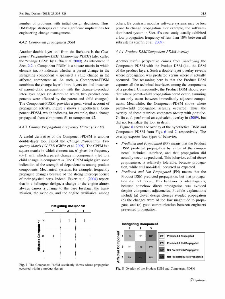
4.4.2 Component propagation DSM
Another double-layer tool from the literature is the Com-
ponent Propagation DSM (Component-PDSM) (also called
the ‘‘change DSM’’ by Giffin et al. 2009). As introduced in
Sect. 2.2, a Component-PDSM is a square matrix in which
element (m, n) indicates whether a parent change in the
instigating component n spawned a child change in the
affected component m. As such, a Component-PDSM
combines the change layer’s intra-layers (to find instances
of parent–child propagation) with the change-to-product
inter-layer edges (to determine which two product com-
ponents were affected by the parent and child changes).
The Component-PDSM provides a great visual account of
propagation activity. Figure 7 shows a hypothetical Com-
ponent-PDSM, which indicates, for example, that a change
propagated from component #1 to component #2.
4.4.3 Change Propagation Frequency Matrix (CPFM)
A useful derivative of the Component-PDSM is another
double-layer tool called the Change Propagation Fre-
quency Matrix (CPFM) (Giffin et al. 2009). The CPFM is a
square matrix in which element (m, n) gives the frequency
(0–1) with which a parent change in component n led to a
child change in component m. The CPFM might give some
indication of the strength of dependencies among product
components. Mechanical systems, for example, frequently
propagate changes because of the strong interdependence
of their physical parts. Indeed, Eckert et al. (2004) reports
that in a helicopter design, a change to the engine almost
always causes a change to the bare fuselage, the trans-
mission, the avionics, and the engine auxiliaries, among
others. By contrast, modular software systems may be less
prone to change propagation. For example, the software-
dominated system in Sect. 5’s case study usually exhibited
a low propagation frequency of less than 10% between all
subsystems (Giffin et al. 2009).
4.4.4 Product DSM/Component-PDSM overlay
Another useful perspective comes from overlaying the
Component-PDSM with the Product DSM (i.e., the DSM
of the product layer). Such a double-layer overlay reveals
where propagation was predicted versus where it actually
occurred. The reasoning here is that the Product DSM
captures all the technical interfaces among the components
of a product. Consequently, the Product DSM should pre-
dict where parent–child propagation could occur, assuming
it can only occur between immediately adjacent compo-
nents. Meanwhile, the Component-PDSM shows where
parent–child propagation actually occurred. Thus, the
overlay of these matrices compares theory with practice.
Giffin et al. performed an equivalent overlay in (2009), but
did not formalize the tool in detail.
Figure 8 shows the overlay of the hypothetical DSM and
Component-PDSM from Figs. 6 and 7, respectively. The
overlay exposes four types of behavior:
• Predicted and Propagated (PP) means that the Product
DSM predicted propagation by virtue of the compo-
nents’ technical interface, and that propagation did
actually occur as predicted. This behavior, called direct
propagation, is relatively tolerable, because propaga-
tion, while still non-ideal, occurred as expected.
• Predicted and Not Propagated (PN) means that the
Product DSM predicted propagation, but that propaga-
tion did not occur. This behavior is advantageous,
because somehow direct propagation was avoided
despite component adjacencies. Possible explanations
include (a) clever design choices avoided propagation
(b) the changes were of too low magnitude to propa-
gate, and (c) good communication between engineers
prevented propagation.
Fig. 7 The Component-PDSM succinctly shows where propagation
occurred within a product design Fig. 8 Overlay of the Product DSM and Component-PDSM
Res Eng Design (2012) 23:305–328 315
123
Page 12
• Not Predicted and Propagated (NP) means that the
product DSM did not predict propagation, yet propa-
gation still occurred. This behavior, called indirect
propagation, contradicts the conventional belief that
parent–child propagation can only occur between
adjacent components. One explanation for this behavior
is that the Product DSM is incomplete (i.e., missing
technical interfaces), such that the indirect propagation
is actually just direct propagation in disguise. The
occurrence of indirect propagation will be investigated
further in Sect. 5’s case study.
• Not Predicted and Not Propagated (NN) means that the
product DSM did not predict propagation and propa-
gation did not occur. This behavior is expected and the
least interesting.
Given any of these behavior types (PP, PN, NP, and
NN), an organization can benefit from investigating their
causes in more depth. When propagation did occur, whe-
ther predicted or not (i.e., PP or NP), the organization
might find ways to improve its operation to avoid propa-
gation in the future. When propagation did not occur (i.e.,
PN or NN), the organization should evaluate the reasons
for the non-propagation of changes and formally adopt or
encourage any good practices.
4.4.5 Alignment matrix
The Alignment Matrix is a double-layer tool developed by
Sosa et al. (2007) that looks for patterns between the
product layer and social layer. The Alignment Matrix
performs an overlay of the Product DSM and the Social
DSM. The premise is that if components a and b are
connected in the Product DSM, then communication
should exist between engineers a and b in the Social DSM.
The Alignment Matrix discovers discrepancies between the
two DSMs for further analysis. One weakness of the
Alignment Matrix is that it is only applicable when there is
a one-to-one mapping between the product and the orga-
nization. If a one-to-one mapping does not exist, as may be
the case for large and complex development projects (Sosa
et al. 2000), use of the Alignment Matrix is not as
straightforward. However, Eppinger (2001) and Morelli
et al. (1995) have found successful workarounds in similar
situations.
In general, the Alignment Matrix exposes two types of
mismatches: unidentified interfaces and unattended inter-
faces, between the Product and Social DSMs (Sosa et al.
2007). An unidentified interface is a communication link
lacking a corresponding product interface, while an unat-
tended interface is a product interface lacking a corre-
sponding communication link. Unidentified interfaces are
generally positive phenomena, while unattended interfaces
can be detrimental when critical product interfaces go
unnoticed. A lack of necessary communication can lead to
poor initial designs that need changing later.
4.4.6 Component-CPI
The first of the double-layer metrics is the Component
Change Propagation Index (Component-CPI, formerly just
‘‘CPI’’), which quantifies a product component’s propaga-
tion behavior. As defined by Suh and de Weck (2007) and
refined by Giffin et al. (2009), the index is calculated by
Eq. 3.
Component-CPIðkÞ ¼ CoutðkÞ � CinðkÞCoutðkÞ þ CinðkÞ
ð3Þ
Through Eq. 3, the Component-CPI compares the numbers
of changes propagating in (Cin(k)) and out (Cout(k)) of a
component. One can determine these quantities from the
multilayer network model. For example, if change n1
spawns change n2 (as would be indicated by an intra-layer
edge between nodes n1 and n2 in the change layer) and
changes n1 and n2 affect components k1 and k2, respec-
tively, (as would be indicated by inter-layer edges con-
necting n1 to k1 and n2 to k2), then Cin(k2) and Cout(k1)
would each be incremented by 1.
The Component-CPI’s quantitative spectrum (-1 to 1)
corresponds with the qualitative behavior spectrum (Sect.
2.1) proposed by Eckert et al. (2004). For example, a mul-
tiplier component gives rise to more changes than it absorbs,
which means Cout(k) [ Cin(k), or CPI [ 0. Meanwhile, a
component could also be a carrier (CPI & 0), absorber
(CPI \ 0), or constant (CPI undefined). Giffin et al. (2009)
considered the distribution of CPI values in a real-world
system of 46 subsystems (see Sect. 5’s case study). They
reported the existence of 7 strong multipliers (CPI [ 0.3), 3
weak multipliers (0.1 \ CPI \ 0.3), 6 carriers (-0.1 \CPI \ 0.1), 13 weak absorbers (-0.3 \ CPI \ -0.1), 13
strong absorbers (CPI \ -0.3), and 4 constants (CPI
undefined).
Suh and de Weck (2007) use the Component-CPI as a
basis for embedding flexibility in a design. For instance,
they recommend that multipliers (and sometimes carriers)
are prime targets for flexibility in anticipation of potentially
costly propagation behavior by these components.
4.4.7 Change acceptance/reflectance rate
Giffin et al. (2009) also defined another double-layer metric
called the Change Acceptance Index (CAI). CAI is the
fraction of proposed changes ultimately accepted by a
product component. The CAI of component k is calculated
by Eq. 4.
316 Res Eng Design (2012) 23:305–328
123
Page 13
CAIðkÞ ¼ Total # of Changes Accepted by Component k
Total # of Changes Proposed for Component k
ð4Þ
The related Change Reflection Index (CRI) of component k
is calculated similarly in Eq. 5.
CRIðkÞ ¼ Total # of Changes Rejected by Component k
Total # of Changes Proposed for Component k
ð5Þ
One can calculate a component’s CAI and CRI from the
multilayer network model. For example, if x changes have
been proposed for component k, then inter-layer edges
would connect x changes in the change layer to component
k in the change layer. The CAI and CRI would then reflect
how many of those x changes were accepted and rejected,
respectively.
The CAI and CRI measure a component’s openness and
stubbornness to accommodate change, respectively. Giffin
et al.’s (2009) study of a real-world system revealed that
the large majority of subsystems were relatively accepting
of change (CAI [ CRI).
4.4.8 Proposal acceptance rate
Another double-layer metric, called the Proposal Accep-
tance Rate (PAR), measures an engineer’s performance as
a proposer of change. Such a metric was suggested by
Giffin (2007), but not developed in detail. When an engi-
neer proposes a change request, the request is ultimately
accepted or rejected. The PAR is essentially an engineer’s
rate of acceptance as a proposer of changes. The PAR of
engineer m can be intuitively calculated with Eq. 6.
PARðmÞ
¼ Total # of Changes Proposed by Engineer m and Accepted
Total # of Changes Proposed by Engineer m
ð6Þ
One can calculate an engineer’s PAR from the multilayer
network model. For example, if engineer m proposed
x changes, then inter-layer edges would connect engineer
m in the product layer to x changes in the change layer. The
PAR would then reflect how many of those x changes were
accepted.
An engineer’s PAR can reflect his or her skill, attitude,
and expertise. A high PAR might mean the engineer is
innovative and knowledgeable, while a low PAR might
imply he or she tends to have ideas that are difficult to
implement. However, other rationalizations for the PAR of
a particular engineer could exist. For instance, a truly
innovative engineer could still have a low PAR if the
organization or product is sluggish or stubborn to make
changes. Conversely, a less creative engineer could still
have a high PAR if the organization or product is especially
receptive of change. Section 5’s case study will explore
these competing explanations using PAR values calculated
for a real-world scenario.
4.5 Triple-layer tools and metrics
Triple-layer tools and metrics consider all three layers of
the multilayer network model at once. Only one triple-layer
tool (the ESM) and one triple-layer metric (graph proper-
ties) were found in the literature.
4.5.1 Engineering systems matrix
As introduced in Sect. 2, Bartolomei’s (2007) ESM is
essentially a DSM augmented to include nodes from mul-
tiple domains and edges within and across those domains.
As such, the ESM can be a triple-layer tool. The ESM
highlights that the multilayer network essentially forms a
single grand network with multiple types of nodes and
edges (similar to a multipartite graph, Diestel 2005).
4.5.2 Graph properties
Just as graph properties were applicable to any single layer,
they can also help describe the grand network formed by all
three layers. In the context of the grand network, all nodes
and edges are treated equally. Consequently, the graph
properties of individual nodes take on new meaning in the
grand network relative to their properties in their respective
single-layer domains. Overall, graph properties of the
grand network, such as centrality, can provide useful
insights into the relative influence of items in the grand
scheme of engineering change management. For instance,
an organization could look for components of high cen-
trality in the grand network to find critical spots in the
product. A highly central component is likely the subject of
extensive change. The organization may consider rede-
signing or buffering that component, so that it does not
consume so much time, money, and resources in the future.
Similarly, an engineer of high centrality in the grand net-
work is likely a systems engineer, high performer, or go-to
person in the organization. By contrast, an engineer of low
centrality might be a specialist, an underperformer, or
someone who is underutilized or only partially assigned to
the project.
4.6 New tools and metrics
Thus far, previous research has provided a good number of
tools and metrics applicable to the multilayer network
model. However, the repository still seems to have a few
Res Eng Design (2012) 23:305–328 317
123
Page 14
weak areas, particularly if one wishes to analyze the social
layer. Indeed, the literature on change propagation has
lacked substantial quantitative treatment for the people
involved in the change process. This paper establishes a
couple of new tools and metrics for this very purpose: the
Engineer Propagation DSM and the Engineer Change
Propagation Index. Another new item introduced here is a
metric called Propagation Directness, which counts how
many technical interfaces are spanned by an instance of
parent–child propagation. These new additions to the
repository are summarized in Table 4.
4.6.1 Engineer propagation DSM
One goal of this research was to determine a way to ana-
lyze the propagation effects of the social layer. To this end,
this paper proposes a double-layer tool called the Engineer
Propagation DSM (Engineer-PDSM).
The Engineer-PDSM tracks instances of change propa-
gation from one engineer to another over some time period
in the design process. The matrix is square with a row
(m) and column (n) for each engineer in an organization.
Element (m, n) of the Engineer-PDSM counts the number
of times a parent change implemented by the instigating
engineer n spawned a child change implemented by the
affected engineer m.
Figure 9 shows the Engineer-PDSM corresponding to
the three engineers (John, Susan, and David) from the
hypothetical application in Sect. 3.2. The matrix indicates
that parent–child propagation occurred twice. One change
propagated from David to Susan, i.e., when David changed
xc, Susan had to change to C1. Another change propagated
from Susan to himself, i.e., when Susan changed C1, she
also had to change C2. It should be noted that David’s
change initially triggered a change for John to implement
as well. However, because John’s change (to R1) was
ultimately rejected, propagation technically did not occur.
Consequently, that rejected propagation does not appear in
the Engineer-PDSM. This convention is also followed by
Giffin et al. (2009).
4.6.2 Engineer-CPI
The Engineer-PDSM can be used to calculate a meaning-
ful double-layer metric called the Engineer Change
Propagation Index (Engineer-CPI). The Engineer-CPI
quantifies an engineer’s performance with respect to the
propagation effects of his (or her) implementation of
changes. The Engineer-CPI is a number between -1 and
?1, calculated by Eq. 7.
Engineer-CPIðmÞ ¼ EoutðmÞ � EinðmÞEoutðmÞ þ EinðmÞ
ð7Þ
In Eq. 7, Eout(m) is the number of changes implemented by
any engineer (including engineer m) that propagated from
changes implemented by engineer m. Ein(m) is the number
of changes implemented by engineer m that propagated
from changes implemented by any engineer (including
engineer m). More simply, Ein(j) and Eout(j) are the
in-degree and out-degree, respectively, of the Engineer-
PDSM. Returning to the hypothetical application, one can
calculate the Engineer-CPIs of David, Susan, and John to
be 1, 0, and undefined, respectively.
It should be obvious that the Engineer-PDSM and
Engineer-CPI are basically extensions of Giffin et al.’s
(2009) Component-PDSM and Component-CPI, respec-
tively. Just as the Component-PDSM captures the occur-
rence of change propagation between product components,
the Engineer-PDSM captures the occurrence of change
propagation between the engineers implementing those
changes. As such, the Engineer-CPI spectrum can be
interpreted similarly to the Component-CPI spectrum;
namely positive, negative, zero, and undefined Engineer-
CPIs correspond with multipliers, absorbers, carriers, and
constants, respectively.
This paper proposes further that the Engineer-CPI
spectrum should also map onto the spectrum of organiza-
tional roles. That is, an engineer’s CPI should theoretically
correspond with his or her job description. Managers and
systems engineers will typically be multipliers (Eout [ Ein)
because they initiate high-level changes that potentially
require many lower-level changes to be completed. For
example, a manager might coordinate with customers and
consequently change the requirements for a product to
Table 4 Newly introduced multilayer network tools and metrics
Name Layers
Tools Engineer propagation DSM Social & change
Metrics Engineer change Propagation Index Social & change
Propagation Directness Change & product
Fig. 9 Engineer propagation DSM for hypothetical application
318 Res Eng Design (2012) 23:305–328
123
Page 15
satisfy. Similarly, a systems engineer might recognize a
high-level problem (e.g., given unsatisfactory test results)
and consequently initiate corrective action that propagates
through the product. By contrast, specialists tend to behave
like absorbers (Ein [ Eout), because they perform changes
in detailed areas of the product where there is little chance
of further propagation. Specialists essentially implement
changes at the end of propagation chains. Meanwhile, team
leaders might correspond with carriers (Ein = Eout), since
they pass on some high-level changes and may initiate
changes on their own, but are also involved with low-level
changes in the product. Finally, constants (Ein = Eout = 0)
do not seem to have an obvious corresponding organiza-
tional role. If an engineer is a constant, that means he (or
she) only implements isolated changes (i.e., they have no
parent change and no children changes) or they are not
involved in engineering change activity at all. An inter-
pretation of this behavior might be a good topic for future
research. Section 5’s case study explores the Engineer-CPI
in greater detail.
4.6.3 Propagation Directness
Propagation Directness (PD) is another double-layer
metric proposed for the first time here. PD is defined as the
number of product interfaces spanned by an instance of
parent–child propagation. PD can be calculated using the
Component-PDSM and Product DSM. Specifically, if the
Component-PDSM indicates that a change propagated
from component n to component m, then the PD of that
propagation is equal to the geodesic (shortest) path from
component n to m in the Product DSM.
Propagation Directness reflects whether propagation is
direct or indirect. Direct propagation implies PD B 1,
because direct propagation occurs when a child change
arises in a component that is adjacent (PD = 1) or identical
(PD = 0) to the component affected by the parent change.
By contrast, indirect propagation has PD [ 1, because a
child change arises in a component nonadjacent to the
component affected by the parent change. As mentioned in
Sect. 4.4.4, direct and indirect propagation correspond with
the PP and NP behavior types, respectively, that may be
exposed when overlaying the Product DSM with the
Component-PDSM.
Propagation Directness has obvious implications for the
successful prediction of change propagation. Conventional
wisdom says that Propagation Directness should always be
PD B 1; in other words, all propagation should be direct
propagation. Accordingly, the CPM suite (Clarkson et al.
2004; Keller et al. 2005) notably only allows for direct
propagation, but emphasizes that recursive direct propa-
gation can form propagation chains spanning several
product interfaces. However, the program in Sect. 5’s case
study experienced a considerable amount of indirect
propagation, in which Propagation Directness was usually
PD = 2 and occasionally PD = 3.
5 Case study
The case under investigation here is that of a large tech-
nical program whose purpose was to develop a large-scale
sensor system. The system consisted of globally distributed
hardware and software segments. The entire endeavor was
very complex and involved multiple stakeholders and dis-
tributed users and operators.
The software-dominated system can be decomposed into
46 areas, or coherent segments of software, hardware, and
different levels of associated documentation. These
‘‘areas’’ are roughly analogous to subsystems, the identities
of which are abstracted in this paper for confidentiality
reasons. Some additional facts about the system were
provided through interviews with one of the program’s lead
systems engineers.
5.1 The data
The data for this case study were extracted from the pro-
gram‘s configuration management records. Details about
the data extraction methodology can be found in Giffin
et al.’s (2009) previous analysis of the same program. The
full extracted dataset contains detailed information about
41,551 change requests (CRs) generated by the program
over an 8-year period. Each CR has a separate record, an
example of which is shown in Table 5. The data entries for
each CR include:
• Identification Number the CR’s unique tracking number
assigned in chronological order
Table 5 Sample change request record
ID number 11520
Data created, last updated MAR-Y6, DEC-Y6
Area affected 1
Change magnitude 0
Parent ID 10506
Children ID(s) 14155
Sibling ID(s) 11685
Submitter Engineer 100
Assignee(s) Engineers 46, 100, 4
Associated individual(s) Engineer 14, 46, 48, 67, 100
Stage, defect, severity –
Completed? 1
Res Eng Design (2012) 23:305–328 319
123
Page 16
• Date Created the month and year that the CR was first
entered in the change management system
• Data Last Updated the month and year that the CR’s
record was last updated
• Area the system area (1 of 46) affected by the CR
• Change Magnitude the expected effort required to
evaluate and implement the CR on a scale of 0–5, based
on the number of source lines of code affected or total
hours required
• Parent ID the ID of the CR’s parent CR, if any
• Children ID(s) the ID(s) of the CR’s children CRs, if
any
• Sibling ID(s) the ID(s) of the CR’s sibling CRs,
including children of the same parent or CRs related in
some other significant way
• Submitter the individual who first entered the CR into
the change management system
• Assignees the individual(s) who formally possessed
responsibility for the CR at some point, either as an
evaluator or implementer
• Associated Individuals other individuals involved with
the CR
• Stage Originated, Defect Reason, & Severity an indi-
cation of whether the CR originated from a documented
customer request; often left blank
• Completed? the approval status of the CR, i.e., accepted
(1), rejected (-1), or still pending (0)
5.2 Model construction
Hidden in the raw data is a very complex multilayer net-
work. In all, the dataset identifies 46 system areas, 41,551
change requests, and 501 engineers and administrators that
constitute the nodes of the product layer, change layer, and
social layer, respectively. The dataset also provides infor-
mation on some, but not all, of the types of intra-layer and
inter-layer edges. Table 6 indicates which edge data were
available for this case study and the source of that data. Of
the intra-layer edges, only those in the product layer and
change layer were available. The product layer’s intra-
layer edges were provided by one of the program’s lead
systems engineers, while the change layer’s intra-layer
edges (i.e., propagation relationships) were gleaned from
the ‘‘Parent ID,’’ ‘‘Children ID(s),’’ and ‘‘Sibling ID(s)’’
entries for each CR record (Table 5). Of the inter-layer
edges, only the change-to-product and social-to-change
inter-layer edges were known, which were gleaned from
the ‘‘Area Affected’’ and ‘‘Assignee(s)’’ (and ‘‘Submitter’’)
entries for each CR record, respectively.
Using the available data, Figs. 10 and 11 draw the
multilayer networks associated with two stand-alone
change networks from the dataset called 11-CR and 87-CR,
respectively. The 11-CR network consists of 11 related
change requests evaluated and implemented by nine engi-
neers and affecting only three of the 46 system areas. The
87-CR network consists of 87 related change requests
evaluated and implemented by 50 engineers and affecting
12 system areas. All the node labels correspond exactly
with those in the raw dataset. For visual ease, the edge
arrows (and node labels for 87-CR) have been removed. No
intra-layer edges are shown in the social layer because the
data were unavailable (Table 6).
5.3 Analysis of engineer performance
The first thrust of this case study elucidates some inter-
esting aspects of the social layer and its influence on
change propagation and the change process. Specifically,
the program’s engineers are analyzed as implementers and
proposers of change using the Engineer-CPI and Proposal
Acceptance Rate, respectively.
5.3.1 Implementers of change
One element of an engineer’s work is the implementation
of changes. To assess an engineer’s performance in this
regard, this case study uses the newly proposed Engineer-
CPI. Figure 12a shows the distribution of Engineer-CPIs
calculated for all 501 engineers identified in the dataset.
The bars do not sum to 501, because nearly half of the
engineers (226) actually behaved like constants (i.e., CPI
undefined) who were only involved with isolated changes,
i.e., they did not contribute to any change propagation.
The authors postulated earlier that the Engineer-CPI
should correspond to the organizational role of an engineer,
i.e., systems engineers are multipliers (CPI [ 0), team
leads are carriers (CPI = 0), and specialists are absorbers
(CPI \ 0). The data confirm this intuition. To determine
the effects of an engineer’s organizational role on his
Engineer-CPI, the engineers in this program were divided
into two classes: coders and testers/integrators. Coders
were the specialists who actually made changes to lines of
code within the system’s software areas. By contrast, tes-
ters and integrators were more like systems engineers who
tested and integrated the system areas together. In the
Table 6 Data availability for case study
Edge data Available? Source
Intra-layer Product layer Yes Interview
Change layer Yes Table 5
Social layer No –
Inter-layer Social-to-change Yes Table 5
Change-to-product Yes Table 5
Product-to-social No –
320 Res Eng Design (2012) 23:305–328
123
Page 17
absence of a detailed project directory, it was still possible
to roughly classify each engineer according to a heuristic
recommended by the lead systems engineer interviewed in
this study. The heuristic classified an engineer as a ‘‘coder’’
if 60% or more of his work focused on core technology in
the system (as opposed to support structure, testing tools,
etc.). Otherwise, the engineer was classified as a ‘‘tester/
integrator.’’
Figure 12b, c show the distribution of Engineer-CPIs for
the coders and testers/integrators, respectively. The distri-
butions offer some evidence that the Engineer-CPI indeed
corresponds with an engineer’s organizational role. As
expected, the coders’ distribution is heavy on the absorber
end of the spectrum. In fact, 74% of coders had negative
CPIs. By contrast, the testers/integrators’ distribution is
heavy on the multiplier end of the spectrum, with 53%
having positive CPIs. The average coder’s CPI was -0.16
(weak absorber), while the average tester/integrator’s CPI
was 0.13 (weak multiplier). Thus, this case study offers
some verification of the correspondence between the
Engineer-CPI and organizational roles, namely the coders
(or specialists) tended to be absorbers, while the testers and
integrators (or ‘‘systems’’ engineers) tended to be multi-
pliers of change.
The data also suggest that another influence on an
engineer’s CPI is the context of his work, i.e., the propa-
gation behavior of the areas to which an engineer is
assigned to implement changes. The rationale here is that
some engineers may be assigned to parts of the product that
are inherently multipliers or inherently absorbers, as
Fig. 10 Multilayer network
model for 11-CR
Fig. 11 Multilayer network
model for 87-CR
Res Eng Design (2012) 23:305–328 321
123
Page 18
measured by their Component-CPIs. As a result, these
engineers may have little independent control over the
propagation effects of their work.
To determine the effect of Component-CPIs on the
Engineer-CPI, the engineers in this program were divided
in two groups: those with absorber assignments and those
with multiplier assignments. An engineer was said to have
‘‘absorber assignments’’ if the average Component-CPI of
his assigned areas was negative (i.e., an absorber). Con-
versely, an engineer was said to have ‘‘multiplier assign-
ments’’ if the average Component-CPI of his assigned areas
was positive (i.e., a multiplier).
Figure 12d, e show the distribution of Engineer-CPIs for
the engineers with absorber and multiplier assignments,
respectively. The distributions offer some evidence that the
Engineer-CPI indeed depends on the Component-CPI of an
engineer’s assigned areas. In fact, 67% of engineers with
absorber assignments had negative CPIs (i.e., were
absorbers), and 75% of engineers with multiplier assign-
ments had positive CPIs (i.e., were multipliers). The
average CPI for each group was -0.12 (weak absorber)
and 0.44 (moderate multiplier), respectively. Thus, an
engineer’s CPI appears to be somewhat dictated by the
Component-CPIs, of his assigned areas. That is, those
engineers who work on multipliers and absorbers tend to be
multipliers and absorbers themselves, respectively.
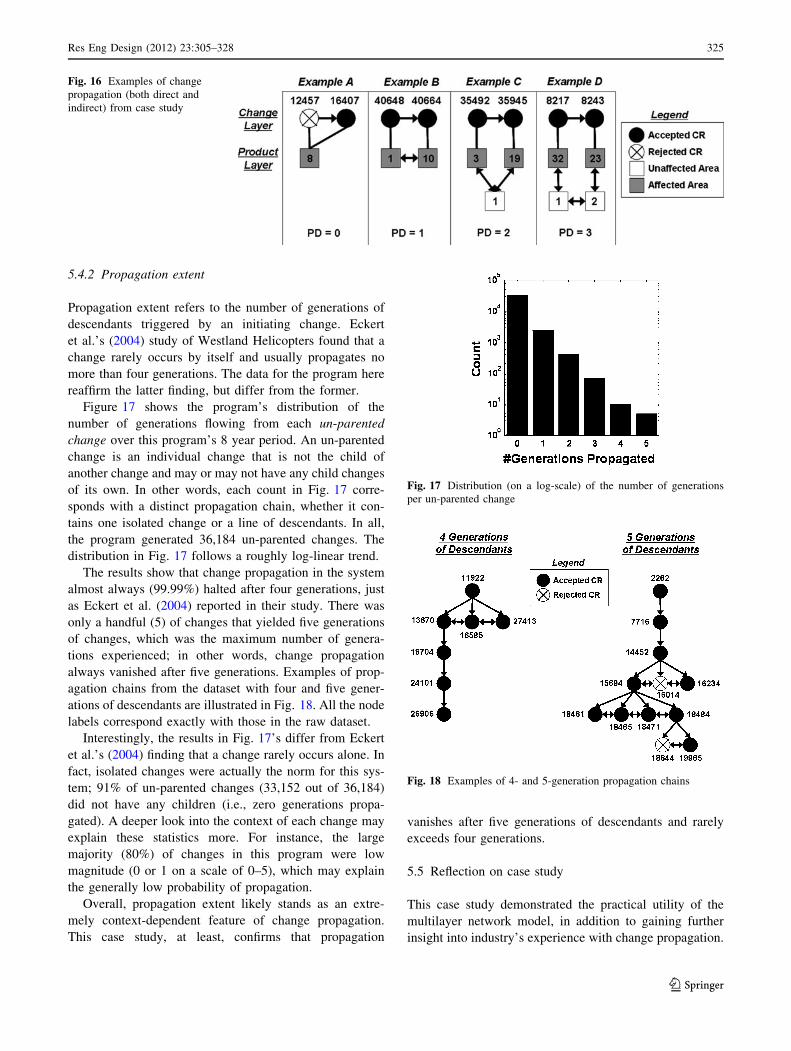
5.3.2 Proposers of change
The other element of an engineer’s work is the proposal of
changes. An engineer CR will ultimately be accepted or
rejected, depending on its costs, benefits, and risks from a
systems perspective. The authors propose a two-dimen-
sional scale for judging the performance of engineers as
proposers of change. The scale’s two dimensions are an
engineer’s proposal acceptance rate (PAR) and the number
of changes he/she proposed.
Figure 13a plots the position of the 382 engineers who
proposed any changes on this scale. Following the advice
of one of the program’s lead systems engineer, Fig. 13a is
additionally broken into four quadrants, A, B, C, and D,
which contain 85 (22%), 151 (40%), 123 (32%), and 23
(6%) of the 382 engineers, respectively The quadrant
boundaries are located at the average PAR and average
proposal count of all 382 data points. Each quadrant has
different implications for an engineer’s performance,
depending on his/her PAR and proposal count relative to
the average engineer:
Fig. 12 Distributions of Engineer-CPIs for various groups of engineers
Fig. 13 Proposal Acceptance
Rate (PAR) results. Each dot in
a represents the position of one
engineer in the program
322 Res Eng Design (2012) 23:305–328
123
Page 19
• Quadrant A contains engineers with high PARs and
high numbers of proposals. These engineers might be
termed ‘‘high performers.’’
• Quadrant B contains engineers with high PARs but low
numbers of proposals. These engineers likely have
great ideas and good systems awareness, since their
change requests are usually accepted. However, for
some reason, they propose a relatively low number of
change requests. The reason for the low proposal count
may lie in the engineer’s organizational role, person-
ality, or some other factor.
• Quadrant C contains engineers with low PARs and low
numbers of proposals. These engineers are relatively
passive with only moderate activity level and little
success as proposers of change.
• Quadrant D contains engineers with low PARs but high
numbers of proposals. There are two possible explana-
tions for this troubling behavior. One is that these
engineers tend to have lots of ideas that are ultimately
rejected because the proposals are not well conceived.
The alternative explanation is that the engineer is
actually quite innovative, but the organization or
product itself is stubborn or sluggish to change.
Whatever the explanation, these engineers should be
managed in a more focused way since they generate
many change requests—each of them causing some
effort for proper review and disposition—but a
substantial fraction of them are not implemented.
Lastly, the authors propose another useful metric, RPAR,
which is the ratio of an engineer’s PAR to the average CAI
of the areas targeted by his change proposals. The ratio is
calculated by Eq. 8, where N is the number of proposed
change requests and CAIn is the CAI of the area targeted by
the nth proposal.
RPAR ¼PAR
1N
PN1 CAIn
ð8Þ
Figure 13b displays a histogram of RPAR values for all the
engineers in the program. The majority (78%) of engineers
have an RPAR & 1, which would indicate that most engi-
neers’ PARs match closely with the CAIs of their under-
lying assigned technical areas. A closer look at the data
reveals that this result is an artifact of most engineers
always proposing change requests in the same area. Con-
sequently, the PARs and associated CAIs are essentially
equal (RPAR = 1). Still, 15% of engineers had RPAR [ 1.
These engineers were able to achieve PARs higher than the
average CAI of their targeted areas. These engineers may
be particularly innovative since their ideas were accepted
by relatively change-resistant areas in the system. By
contrast, the 10% of engineers with RPAR \ 1 struggled to
get changes accepted by relatively receptive areas. These
engineers may not be quite as innovative or systems savvy
and might benefit from additional training.
5.4 Characterization of change propagation
The second thrust of this case study involves the general
characterization of change propagation. The primary issue
addressed here is the counterintuitive phenomenon of
indirect propagation, a common occurrence for this pro-
gram. Secondly, the study considers the issue of propa-
gation extent, the number of generations of descendants
propagated by an initiating change. In this program,
propagation always stopped after five, and rarely more than
four, generations of descendants.
5.4.1 Indirect propagation
Conventional wisdom about change propagation assumes
that only direct propagation is possible; that is, a parent
change in one component can only yield child changes in
itself or immediately adjacent components (Clarkson et al.
2004). However, the program discussed here experienced
considerable indirect propagation, whereby child changes
occurred in nonadjacent areas.
Figure 14 overlays the program’s Product DSM with its
Component-PDSM (from Sect. 4.4.4). Giffin et al. (2009)
performed an equivalent overlay for this program. The
overlay exposes all four types of parent–child propagation
behavior. Overall, 15, 9, 9, and 66% of all pairs of com-
ponents exhibited PP, PN, NP, and NN behavior,
respectively.
Where propagation did occur (PP and NP), it is mean-
ingful to calculate the effective Propagation Directness
(from Sect. 4.6.3). Figure 15 displays the distribution of
Propagation Directness values, considering every instance
of parent–child propagation in the program in which the
child change was accepted (regardless of the parent chan-
ge’s approval status). The distribution reveals that 78% of
all parent–child propagation in the program was direct
(PD B 1), while a surprising 22% was indirect (PD [ 1).
The vast majority of indirect propagation occurred across
two interfaces (PD = 2) and a handful (3) occurred across
three interfaces (PD = 3). It should be noted that the
maximum possible Propagation Directness was three
because the system network’s diameter is three.
Delving further, Fig. 16 illustrates a few examples of
parent–child propagation from the dataset. In each illus-
tration, the change layer contains the parent change and
child change connected by a directed intra-layer edge.
Meanwhile, inter-layer edges connect these changes to the
affected areas in the product layer. For PD [ 1, the product
layer also contains the unaffected areas on the shortest path
between the two affected areas. All nodes are labeled as
Res Eng Design (2012) 23:305–328 323
123
Page 20
they appear in the raw data. For simplicity, the social layer
is omitted.
Each example in Fig. 16 has a different Propagation
Directness value, which should be clear from the number of
product interfaces spanned by the propagation. In Example
A, self-propagation (PD = 0) occurred in Area #8; inter-
estingly, the parent change in this example was ultimately
rejected. Next, Example B shows direct propagation
between adjacent areas (PD = 1); a change to Area #1,
which contains requirements documentation, caused a
change in Area #10, a core technology area. Example C
exhibits indirect propagation; Areas #3 and #19 are sepa-
rated by two interfaces (PD = 2) with Area #1 in between
them. It should be noted that several geodesic (length-2)
paths exist between Areas #3 and #19, besides the one
through Area #1. Finally, Example D shows one of only
three scenarios in the entire dataset with PD = 3. It is
important to remember that in Examples C and D, the
intermediate areas (connecting the two affected areas) were
unaffected by any related change, which constitutes indi-
rect propagation.
The phenomenon of indirect propagation contradicts
conventional wisdom on change propagation. As such, one
might conclude that if indirect propagation appears to have
occurred, then the Product DSM must be missing some
interfaces that actually exist; in other words, any observed
indirect propagation is really direct propagation in dis-
guise. If this explanation is true, then the Product DSM in
this case study would shockingly be missing 192 inter-
faces. This seems unlikely. In fact, a lead systems engineer
from the program explained that indirect propagation is a
legitimate artifact of software system development.
Apparently, engineers in this program would frequently
violate the intended structure of the system in order to
achieve a quick solution for a redesign. These ill-advised
maneuvers were sometimes necessary during time crun-
ches to meet development milestones (e.g., PDR, CDR).
For example, one area of the system contained system
adjustable parameters (SAPs). A SAP is a system variable
kept in a loadable file, rather than in the software code
itself. Many areas of the system were nominally discon-
nected from the SAP file. Still, on occasion, a hasty
redesign effort would change the SAP file (e.g., adding an
SAP), despite the lack of an interface between the SAP file
and the parent area. In effect, a new interface was created,
allowing a change to propagate; however, this interface
was not part of the original Product DSM. Thus, indirect
propagation, though unintended, can and does occur during
product development. Additional case studies are neces-
sary to determine whether indirect propagation is a com-
mon artifact among software systems only, or hardware
systems as well.
Fig. 14 Overlay of Product and
Component-PDSM for case
study
Fig. 15 Distribution of Propagation Directness
324 Res Eng Design (2012) 23:305–328
123
Page 21
5.4.2 Propagation extent
Propagation extent refers to the number of generations of
descendants triggered by an initiating change. Eckert
et al.’s (2004) study of Westland Helicopters found that a
change rarely occurs by itself and usually propagates no
more than four generations. The data for the program here
reaffirm the latter finding, but differ from the former.
Figure 17 shows the program’s distribution of the
number of generations flowing from each un-parented
change over this program’s 8 year period. An un-parented
change is an individual change that is not the child of
another change and may or may not have any child changes
of its own. In other words, each count in Fig. 17 corre-
sponds with a distinct propagation chain, whether it con-
tains one isolated change or a line of descendants. In all,
the program generated 36,184 un-parented changes. The
distribution in Fig. 17 follows a roughly log-linear trend.
The results show that change propagation in the system
almost always (99.99%) halted after four generations, just
as Eckert et al. (2004) reported in their study. There was
only a handful (5) of changes that yielded five generations
of changes, which was the maximum number of genera-
tions experienced; in other words, change propagation
always vanished after five generations. Examples of prop-
agation chains from the dataset with four and five gener-
ations of descendants are illustrated in Fig. 18. All the node
labels correspond exactly with those in the raw dataset.
Interestingly, the results in Fig. 17’s differ from Eckert
et al.’s (2004) finding that a change rarely occurs alone. In
fact, isolated changes were actually the norm for this sys-
tem; 91% of un-parented changes (33,152 out of 36,184)
did not have any children (i.e., zero generations propa-
gated). A deeper look into the context of each change may
explain these statistics more. For instance, the large
majority (80%) of changes in this program were low
magnitude (0 or 1 on a scale of 0–5), which may explain
the generally low probability of propagation.
Overall, propagation extent likely stands as an extre-
mely context-dependent feature of change propagation.
This case study, at least, confirms that propagation
vanishes after five generations of descendants and rarely
exceeds four generations.
5.5 Reflection on case study
This case study demonstrated the practical utility of the
multilayer network model, in addition to gaining further
insight into industry’s experience with change propagation.
Fig. 16 Examples of change
propagation (both direct and
indirect) from case study
Fig. 17 Distribution (on a log-scale) of the number of generations
per un-parented change
Fig. 18 Examples of 4- and 5-generation propagation chains
Res Eng Design (2012) 23:305–328 325
123
Page 22
The most valuable and novel part of the study was the
investigation of the largely unexplored social layer. Here,
the Engineer-CPI and PAR showed promise as measures
of personnel management and performance assessment.
The Engineer-CPI was used to quantify the propagation
effects of an engineer’s implementation of changes. The
data indicated that the Engineer-CPI is partially depen-
dent on an engineer’s organizational role and the context
of his assignments. Coders and engineers who worked on
absorbers in the system tended to behave like absorbers
themselves. Meanwhile, testers/integrators and engineers
who worked on multipliers in the system tended to
behave like multipliers themselves. The program’s engi-
neers were also analyzed as proposers of change with
respect to their PAR and the total number of changes they
proposed. A more conscious assignment of roles and
identification of engineers who fall into Quadrant D
(Fig. 13a) may help identify those who might benefit
from additional training.
The case study also contributed to the general charac-
terization of change propagation. It was found that soft-
ware-intensive systems may be particularly susceptible to
indirect propagation, by which changes propagate between
nonadjacent product components. Finally, the study found
that most changes did not lead to any propagation. Prop-
agation that did occur always stopped after five, and rarely
more than four, generations of descendants. The trends
revealed here contribute to the future ability to rank or tag
change requests according to their likelihood of initiating
long propagation chains.
Ideally, the above analyses would have been performed
during the development effort, rather than in post. That
way, the program could have acted on the results. This case
study had the luxury of a rich dataset spanning the full
development effort. However, it is unclear (and not within
the scope of this paper) whether sufficient data would have
been available to reveal any actionable trends in real time.
Nevertheless, the use of retrospective statistical analysis, as
in this case study, still has potential value for future
development efforts. After all, most products (and systems)
are adaptations of predecessors and many are at least
analogous to previous products (Giffin et al. 2009). Con-
sequently, it may be possible to develop heuristic rela-
tionships to predict the expected change activity for a new
product, by analyzing change statistics from analogous
development efforts.
6 Conclusion
This paper presented a multilayer network model of change
propagation in hope of introducing a useful approach to
industry and the research community. Returning to the
research questions of Sect. 1.2, the authors propose the
following answers based on their research findings:
• What insights can be gained from a multilayer network
model of change propagation? A multilayer network
model (Fig. 3) provides a holistic, data-driven frame-
work for analyzing and managing change propagation.
As demonstrated by the case study, new insights are
particularly gained by inclusion of the social layer. The
model represents a data-driven approach to change
management with the potential to guide design strategy,
change impact analysis, and human resource manage-
ment. Only a holistic framework like the multilayer
network model could comprehensively address all these
areas.
• What are potential tools and metrics for analyzing the
model? The multilayer network model provides a
platform for an array of viable tools and metrics. In
Table 2, this paper proposed a baseline repository of
tools and metrics, both old and new. Many tools and
metrics previously proposed in the literature are readily
incorporated by the model. Consequently, the model
offers a comprehensive paradigm that unifies previous
research in a common framework. Moreover, this paper
introduced some promising new tools and metrics,
including the Engineer-PDSM, Engineer-CPI, and
Propagation Directness.
• How can the model contribute to the prevention,
prediction, and control of change propagation? The
multilayer perspective urges an organization to con-
sider the influence of all three layers (product, change,
and social) when trying to prevent, predict, and control
change propagation. The multilayer network model and
repository of tools and metrics (Table 2) provide the
means for executing such a holistic strategy.
For instance, the prevention of change propagation can
be accomplished through effective management of both the
product layer and social layer. Within the product layer, an
organization can embed flexibility in a design to avoid
future change propagation, e.g., by turning multipliers
(CPI [ 0) into absorbers (CPI \ 0) (Suh and de Weck
2007). Within the social layer, an organization can foster
necessary communication between teams and engineers
who are designing interdependent parts of the product.
Consistency between the product layer and social layer, as
checked by the Alignment Matrix (Sosa et al. 2007), is a
critical means of preventing change propagation.
Meanwhile, the prediction of change propagation
requires analysis of the product layer and change layer. A
prediction capability has both tactical and strategic impli-
cations. Tactical prediction is useful in the short term, such
as when an organization assesses the impact of individual
change requests during product development. Tactical
326 Res Eng Design (2012) 23:305–328
123
Page 23
prediction draws on analysis of the product layer through
tools like CPM (Clarkson et al. 2004; Keller et al. 2005).
Meanwhile, strategic prediction has long-term utility, such
as in the estimation of life-cycle costs during the earliest
stages of product development or while negotiating product
requirements with prospective clients. Strategic prediction
requires a fundamental characterization of propagation
behavior in the change layer. Strategic prediction might
draw on the statistical change behavior of analogous pro-
jects to estimate the total amount of change activity
expected for an upcoming project (Sect. 5.5).
Finally, the control of change propagation especially
hinges on the management of the social layer. Section 5.3
of the case study suggests that human resource manage-
ment is a promising element of controlling change propa-
gation. The Engineer-CPI and PAR are examples of
quantitative metrics for evaluating personnel performance
in the implementation and proposal of changes,
respectively.
In summary, a multilayer network view in product
development holds the promise of turning change man-
agement from a rather passive administrative process to a
more holistic, proactive, and data-driven systems engi-
neering process.
6.1 Future work
The multilayer network model creates several avenues for
future work, including the following:
• This paper has only scratched the surface of the social
layer. Many questions remain about the social layer’s
contribution to propagation phenomena. For instance, it
may be insightful to consider an engineer’s CPI with
respect to his or her workload and experience, as well
as human resource management and milestones during
product development.
• Better visualization techniques for the multilayer
network model are needed. Clearer drawings may
reveal patterns and other insights more readily recog-
nized and appreciated by the human brain. The dataset
from this case study provides an array of small and
large change networks to test various multilayer
network visualization techniques in the future.
• One of the chief questions underlying all change
propagation research regards the predictability of
change and change propagation. A multilayer perspec-
tive can aid these future efforts through holistic, data-
driven analysis.
Acknowledgment Excerpts and figures from this paper were pre-
viously published by the Design Society in: Pasqual, MC, de Weck,
OL (2011) Multilayer network model for analysis and management of
change propagation. In: Proceedings of the 18th International Con-
ference on Engineering Design, pp 126–138.
References
Bartolomei J (2007) Qualitative knowledge construction for engi-
neering systems: extending the design structure matrix method-
ology in scope and procedure. Dissertation, Massachusetts
Institute of Technology
Browning TR (2001) Applying the design structure matrix to system
decomposition and integration problems: a review and new
directions. IEEE Trans Eng Manag 48(3):292–306
Clarkson PJ, Simons C, Eckert C (2004) Predicting change propa-
gation in complex design. Trans ASME 126:788–797
Danilovic M, Browning TR (2007) Managing complex product
development projects with design structure matrices and domain
mapping matrices. Int J Manag 25:300–314
Diestel R (2005) Graph theory, 3rd edn. Springer, New York
Earl C, Eckert C, Clarkson J (2005) Design change and complexity.
In: 2nd workshop on complexity in design and engineering
Eckert C, Clarkson P, Zanker W (2004) Change and customization in
complex engineering domains. Res Eng Design 15:1–21
Eppinger SD (2001) Patterns of product development interactions. In:
13th international conference on engineering design
Eppinger S, Whitney D, Smith R, Gebala D (1994) A model-based
method for organizing tasks in product development. Res Eng
Design 6(1):1–21
Giffin M (2007) Change propagation in large technical systems.
Thesis, Massachusetts Institute of Technology
Giffin M, de Weck O, Bounova G, Keller R, Eckert C, Clarkson J
(2009) Change propagation analysis in complex technical
systems. J Mech Des 131(8):081010
Huang GQ, Mak KL (1999) Current practices of engineering change
management in UK manufacturing industries. Int J Oper Prod
Manag 19(1):21
Jarratt T, Eckert C, Clarkson J (2006) Pitfalls of engineering change:
change practice during complex product design. Adv Des
413–424
Keller R, Eger T, Eckert CM, Clarkson PJ (2005) Visualizing change
propagation. In: 15th international conference on engineering
design, pp 62–63
Morelli MD, Eppinger SD, Gulati RK (1995) Predicting technical
communication in product development organizations. IEEE
Trans Eng Manag 42(2):215–222
N.A.S.A. (2007) NASA systems engineering handbook. SP-2007-
6105 R1
Newman J (2003) The structure and function of complex networks.
Soc Ind Appl Math 42(2):167–256
Nichols K (1990) Getting engineering changes under control. J Eng
Des 1(1):1–6
Pikosz P, Malmqvist J (1998) A comparative study of engineering
change management in three Swedish companies. In: Proceed-
ings of the DETC98 ASME design engineering technical
conference, pp 78–85
Sosa ME, Eppinger SD, Rowles CM (2000) Understanding the effects
of product architecture on technical communication in product
development organizations. Massachusetts Institute of Technol-
ogy Sloan School of Management Working Paper 4130
Sosa ME, Eppinger SD, Rowles CM (2007) Are your engineers
talking to one another when they should? Harvard Bus Rev
85(11):133–142
Steward DV (1981) The design structure system: a method for
managing the design of complex systems. IEEE Trans Eng
Manag 28(3):71–74
Res Eng Design (2012) 23:305–328 327
123
Page 24
Suh ES, de Weck OL (2007) Flexible product platforms: framework
and case study. Res Eng Design 18(2):67–89
Terwiesch C, Loch C (1999) Managing the process of engineering
change orders: the case of the climate control system in
automobile development. J Prod Innov Manag 16:160–172
Wright IC (1997) A review of research into engineering change
management: implications for product design. Des Stud
18:33–42
328 Res Eng Design (2012) 23:305–328
123