MULTILINEAR ALGEBRA 1.1 Background - MIT …math.mit.edu/classes/18.952/spring2013/docs/book.pdf ·...

This is page 1Printer: Opaque this

CHAPTER 1

MULTILINEAR ALGEBRA

1.1 Background

We will list below some definitions and theorems that are part ofthe curriculum of a standard theory-based sophomore level coursein linear algebra. (Such a course is a prerequisite for reading thesenotes.) A vector space is a set, V , the elements of which we will referto as vectors. It is equipped with two vector space operations:Vector space addition. Given two vectors, v1 and v2, one can addthem to get a third vector, v1 + v2.Scalar multiplication. Given a vector, v, and a real number, λ, onecan multiply v by λ to get a vector, λv.

These operations satisfy a number of standard rules: associativ-ity, commutativity, distributive laws, etc. which we assume you’refamiliar with. (See exercise 1 below.) In addition we’ll assume you’refamiliar with the following definitions and theorems.

1. The zero vector. This vector has the property that for everyvector, v, v+ 0 = 0+ v = v and λv = 0 if λ is the real number, zero.

2. Linear independence. A collection of vectors, vi, i = 1, . . . , k, islinearly independent if the map

(1.1.1) Rk → V , (c1, . . . , ck) → c1v1 + · · · + ckvk

is 1 − 1.

3. The spanning property. A collection of vectors, vi, i = 1, . . . , k,spans V if the map (1.1.1) is onto.

4. The notion of basis. The vectors, vi, in items 2 and 3 are a basisof V if they span V and are linearly independent; in other words, ifthe map (1.1.1) is bijective. This means that every vector, v, can bewritten uniquely as a sum

(1.1.2) v =∑

civi .

2 Chapter 1. Multilinear algebra

5. The dimension of a vector space. If V possesses a basis, vi,i = 1, . . . , k, V is said to be finite dimensional, and k is, by definition,the dimension of V . (It is a theorem that this definition is legitimate:every basis has to have the same number of vectors.) In this chapterall the vector spaces we’ll encounter will be finite dimensional.

6. A subset, U , of V is a subspace if it’s vector space in its ownright, i.e., for v, v1 and v2 in U and λ in R, λv and v1 + v2 are in U .

7. Let V and W be vector spaces. A map, A : V → W is linear if,for v, v1 and v2 in V and λ ∈ R

A(λv) = λAv(1.1.3)

and

A(v1 + v2) = Av1 +Av2 .(1.1.4)

8. The kernel of A. This is the set of vectors, v, in V which getmapped by A into the zero vector in W . By (1.1.3) and (1.1.4) thisset is a subspace of V . We’ll denote it by “KerA”.

9. The image of A. By (1.1.3) and (1.1.4) the image of A, whichwe’ll denote by “ImA”, is a subspace of W . The following is animportant rule for keeping track of the dimensions of KerA andImA.

(1.1.5) dimV = dim KerA+ dim ImA .

Example 1. The map (1.1.1) is a linear map. The vi’s span V if itsimage is V and the vi’s are linearly independent if its kernel is justthe zero vector in R

k.

10. Linear mappings and matrices. Let v1, . . . , vn be a basis of Vand w1, . . . , wm a basis of W . Then by (1.1.2) Avj can be writtenuniquely as a sum,

(1.1.6) Avj =

m∑

i=1

ci,jwi , ci,j ∈ R .

The m × n matrix of real numbers, [ci,j ], is the matrix associatedwith A. Conversely, given such an m × n matrix, there is a uniquelinear map, A, with the property (1.1.6).

1.1 Background 3

11. An inner product on a vector space is a map

B : V × V → R

having the three properties below.

(a) For vectors, v, v1, v2 and w and λ ∈ R

B(v1 + v2, w) = B(v1, w) +B(v2, w)

and

B(λv,w) = λB(v,w) .

(b) For vectors, v and w,

B(v,w) = B(w, v) .

(c) For every vector, v

B(v, v) ≥ 0 .

Moreover, if v 6= 0, B(v, v) is positive.

Notice that by property (b), property (a) is equivalent to

B(w, λv) = λB(w, v)

and

B(w, v1 + v2) = B(w, v1) +B(w, v2) .

The items on the list above are just a few of the topics in linear al-gebra that we’re assuming our readers are familiar with. We’ve high-lighted them because they’re easy to state. However, understandingthem requires a heavy dollop of that indefinable quality “mathe-matical sophistication”, a quality which will be in heavy demand inthe next few sections of this chapter. We will also assume that ourreaders are familiar with a number of more low-brow linear algebranotions: matrix multiplication, row and column operations on matri-ces, transposes of matrices, determinants of n×n matrices, inversesof matrices, Cramer’s rule, recipes for solving systems of linear equa-tions, etc. (See §1.1 and 1.2 of Munkres’ book for a quick review ofthis material.)


Exercises.

1. Our basic example of a vector space in this course is Rn equipped

with the vector addition operation

(a1, . . . , an) + (b1, . . . , bn) = (a1 + b1, . . . , an + bn)

and the scalar multiplication operation

λ(a1, . . . , an) = (λa1, . . . , λan) .

Check that these operations satisfy the axioms below.

(a) Commutativity: v + w = w + v.

(b) Associativity: u+ (v + w) = (u+ v) + w.

(c) For the zero vector, 0 = (0, . . . , 0), v + 0 = 0 + v.

(d) v + (−1)v = 0.

(e) 1v = v.

(f) Associative law for scalar multiplication: (ab)v = a(bv).

(g) Distributive law for scalar addition: (a+ b)v = av + bv.

(h) Distributive law for vector addition: a(v + w) = av + aw.

2. Check that the standard basis vectors of Rn: e1 = (1, 0, . . . , 0),

e2 = (0, 1, 0, . . . , 0), etc. are a basis.

3. Check that the standard inner product on Rn

B((a1, . . . , an), (b1, . . . , bn)) =n∑

i=1

aibi

is an inner product.

1.2 Quotient spaces and dual spaces

In this section we will discuss a couple of items which are frequently,but not always, covered in linear algebra courses, but which we’llneed for our treatment of multilinear algebra in §§1.1.3 – 1.1.8.

1.2 Quotient spaces and dual spaces 5

The quotient spaces of a vector space

Let V be a vector space and W a vector subspace of V . A W -cosetis a set of the form

v +W = v + w , w ∈W .

It is easy to check that if v1 − v2 ∈ W , the cosets, v1 + W andv2 + W , coincide while if v1 − v2 6∈ W , they are disjoint. Thus theW -cosets decompose V into a disjoint collection of subsets of V . Wewill denote this collection of sets by V/W .

One defines a vector addition operation on V/W by defining thesum of two cosets, v1 +W and v2 +W to be the coset

(1.2.1) v1 + v2 +W

and one defines a scalar multiplication operation by defining thescalar multiple of v +W by λ to be the coset

(1.2.2) λv +W .

It is easy to see that these operations are well defined. For instance,suppose v1 + W = v′1 + W and v2 + W = v′2 + W . Then v1 − v′1and v2 − v′2 are in W ; so (v1 + v2) − (v′1 + v′2) is in W and hencev1 + v2 +W = v′1 + v′2 +W .

These operations make V/W into a vector space, and one callsthis space the quotient space of V by W .

We define a mapping

(1.2.3) π : V → V/W

by setting π(v) = v + W . It’s clear from (1.2.1) and (1.2.2) thatπ is a linear mapping, and that it maps V to V/W . Moreover, forevery coset, v +W , π(v) = v +W ; so the mapping, π, is onto. Alsonote that the zero vector in the vector space, V/W , is the zero coset,0+W = W . Hence v is in the kernel of π if v+W = W , i.e., v ∈W .In other words the kernel of π is W .

In the definition above, V and W don’t have to be finite dimen-sional, but if they are, then

(1.2.4) dimV/W = dimV − dimW .

by (1.1.5).The following, which is easy to prove, we’ll leave as an exercise.


Proposition 1.2.1. Let U be a vector space and A : V → U a linearmap. If W ⊂ KerA there exists a unique linear map, A# : V/W → Uwith property, A = A# π.

The dual space of a vector space

We’ll denote by V ∗ the set of all linear functions, ℓ : V → R. If ℓ1and ℓ2 are linear functions, their sum, ℓ1 + ℓ2, is linear, and if ℓ isa linear function and λ is a real number, the function, λℓ, is linear.Hence V ∗ is a vector space. One calls this space the dual space of V .

Suppose V is n-dimensional, and let e1, . . . , en be a basis of V .Then every vector, v ∈ V , can be written uniquely as a sum

v = c1e1 + · · · + cnen ci ∈ R .

Let

(1.2.5) e∗i (v) = ci .

If v = c1e1 + · · · + cnen and v′ = c′1e1 + · · · + c′nen then v + v′ =(c1 + c′1)e1 + · · · + (cn + c′n)en, so

e∗i (v + v′) = ci + c′i = e∗i (v) + e∗i (v′) .

This shows that e∗i (v) is a linear function of v and hence e∗i ∈ V ∗.

Claim: e∗i , i = 1, . . . , n is a basis of V ∗.

Proof. First of all note that by (1.2.5)

(1.2.6) e∗i (ej) =

1 , i = j0 , i 6= j

.

If ℓ ∈ V ∗ let λi = ℓ(ei) and let ℓ′ =∑λie

∗i . Then by (1.2.6)

(1.2.7) ℓ′(ej) =∑

λie∗i (ej) = λj = ℓ(ej) ,

i.e., ℓ and ℓ′ take identical values on the basis vectors, ej. Henceℓ = ℓ′.

Suppose next that∑λie

∗i = 0. Then by (1.2.6), λj = (

∑λie

∗i )(ej) =

0 for all j = 1, . . . , n. Hence the e∗j ’s are linearly independent.


Let V and W be vector spaces and A : V → W , a linear map.Given ℓ ∈ W ∗ the composition, ℓ A, of A with the linear map,ℓ : W → R, is linear, and hence is an element of V ∗. We will denotethis element by A∗ℓ, and we will denote by

A∗ : W ∗ → V ∗

the map, ℓ→ A∗ℓ. It’s clear from the definition that

A∗(ℓ1 + ℓ2) = A∗ℓ1 +A∗ℓ2

and that

A∗λℓ = λA∗ℓ ,

i.e., that A∗ is linear.

Definition. A∗ is the transpose of the mapping A.

We will conclude this section by giving a matrix description ofA∗. Let e1, . . . , en be a basis of V and f1, . . . , fm a basis of W ; lete∗1, . . . , e

∗n and f∗1 , . . . , f

∗m be the dual bases of V ∗ and W ∗. Suppose A

is defined in terms of e1, . . . , en and f1, . . . , fm by the m×n matrix,[ai,j], i.e., suppose

Aej =∑

ai,jfi .

Claim. A∗ is defined, in terms of f∗1 , . . . , f∗m and e∗1, . . . , e

∗n by the

transpose matrix, [aj,i].

Proof. Let

A∗f∗i =∑

cj,ie∗j .

Then

A∗f∗i (ej) =∑

k

ck,ie∗k(ej) = cj,i

by (1.2.6). On the other hand

A∗f∗i (ej) = f∗i (Aej) = f∗i

(∑ak,jfk

)=∑

k

ak,jf∗i (fk) = ai,j

so ai,j = cj,i.


Exercises.

1. Let V be an n-dimensional vector space and W a k-dimensionalsubspace. Show that there exists a basis, e1, . . . , en of V with theproperty that e1, . . . , ek is a basis of W . Hint: Induction on n − k.To start the induction suppose that n− k = 1. Let e1, . . . , en−1 be abasis of W and en any vector in V −W .

2. In exercise 1 show that the vectors fi = π(ek+i), i = 1, . . . , n−kare a basis of V/W .

3. In exercise 1 let U be the linear span of the vectors, ek+i, i =1, . . . , n− k.

Show that the map

U → V/W , u→ π(u) ,

is a vector space isomorphism, i.e., show that it maps U bijectivelyonto V/W .

4. Let U , V and W be vector spaces and let A : V → W andB : U → V be linear mappings. Show that (AB)∗ = B∗A∗.

5. Let V = R2 and let W be the x1-axis, i.e., the one-dimensional

subspace(x1, 0) ; x1 ∈ R

of R2.

(a) Show that the W -cosets are the lines, x2 = a, parallel to thex1-axis.

(b) Show that the sum of the cosets, “x2 = a” and “x2 = b” is thecoset “x2 = a+ b”.

(c) Show that the scalar multiple of the coset, “x2 = c” by thenumber, λ, is the coset, “x2 = λc”.

6. (a) Let (V ∗)∗ be the dual of the vector space, V ∗. For everyv ∈ V , let µv : V ∗ → R be the function, µv(ℓ) = ℓ(v). Show thatthe µv is a linear function on V ∗, i.e., an element of (V ∗)∗, and showthat the map

(1.2.8) µ : V → (V ∗)∗ v → µv

is a linear map of V into (V ∗)∗.


(b) Show that the map (1.2.8) is bijective. (Hint: dim(V ∗)∗ =dimV ∗ = dimV , so by (1.1.5) it suffices to show that (1.2.8) isinjective.) Conclude that there is a natural identification of V with(V ∗)∗, i.e., that V and (V ∗)∗ are two descriptions of the same object.

7. Let W be a vector subspace of V and let

W⊥ = ℓ ∈ V ∗ , ℓ(w) = 0 if w ∈W .

Show that W⊥ is a subspace of V ∗ and that its dimension is equal todimV −dimW . (Hint: By exercise 1 we can choose a basis, e1, . . . , enof V such that e1, . . . ek is a basis of W . Show that e∗k+1, . . . , e

∗n is a

basis of W⊥.) W⊥ is called the annihilator of W in V ∗.

8. Let V and V ′ be vector spaces and A : V → V ′ a linear map.Show that if W is the kernel of A there exists a linear map, B :V/W → V ′, with the property: A = B π, π being the map (1.2.3).In addition show that this linear map is injective.

9. Let W be a subspace of a finite-dimensional vector space, V .From the inclusion map, ι : W⊥ → V ∗, one gets a transpose map,

ι∗ : (V ∗)∗ → (W⊥)∗

and, by composing this with (1.2.8), a map

ι∗ µ : V → (W⊥)∗ .

Show that this map is onto and that its kernel is W . Conclude fromexercise 8 that there is a natural bijective linear map

ν : V/W → (W⊥)∗

with the property ν π = ι∗ µ. In other words, V/W and (W⊥)∗ aretwo descriptions of the same object. (This shows that the “quotientspace” operation and the “dual space” operation are closely related.)

10. Let V1 and V2 be vector spaces and A : V1 → V2 a linear map.Verify that for the transpose map: A∗ : V ∗

2 → V ∗1

KerA∗ = (ImA)⊥

and

ImA∗ = (KerA)⊥ .


11. (a) Let B : V × V → R be an inner product on V . For v ∈ Vlet

ℓv : V → R

be the function: ℓv(w) = B(v,w). Show that ℓv is linear and showthat the map

(1.2.9) L : V → V ∗ , v → ℓv

is a linear mapping.

(b) Prove that this mapping is bijective. (Hint: Since dimV =dimV ∗ it suffices by (1.1.5) to show that its kernel is zero. Now notethat if v 6= 0 ℓv(v) = B(v, v) is a positive number.) Conclude that ifV has an inner product one gets from it a natural identification ofV with V ∗.

12. Let V be an n-dimensional vector space and B : V × V → R

an inner product on V . A basis, e1, . . . , en of V is orthonormal is

(1.2.10) B(ei, ej) =

1 i = j0 i 6= j

(a) Show that an orthonormal basis exists. Hint: By induction letei, i = 1, . . . , k be vectors with the property (1.2.10) and let v be avector which is not a linear combination of these vectors. Show thatthe vector

w = v −∑

B(ei, v)ei

is non-zero and is orthogonal to the ei’s. Now let ek+1 = λw, where

λ = B(w,w)−1

2 .

(b) Let e1, . . . en and e′1, . . . e′n be two orthogonal bases of V and let

(1.2.11) e′j =∑

ai,jei .

Show that

(1.2.12)∑

ai,jai,k =

1 j = k0 j 6= k

(c) Let A be the matrix [ai,j]. Show that (1.2.12) can be writtenmore compactly as the matrix identity

(1.2.13) AAt = I

where I is the identity matrix.


(d) Let e1, . . . , en be an orthonormal basis of V and e∗1, . . . , e∗n the

dual basis of V ∗. Show that the mapping (1.2.9) is the mapping,Lei = e∗i , i = 1, . . . n.


1.3 Tensors

Let V be an n-dimensional vector space and let V k be the set of allk-tuples, (v1, . . . , vk), vi ∈ V . A function

T : V k → R

is said to be linear in its ith variable if, when we fix vectors, v1, . . . , vi−1,vi+1, . . . , vk, the map

(1.3.1) v ∈ V → T (v1, . . . , vi−1, v, vi+1, . . . , vk)

is linear in V . If T is linear in its ith variable for i = 1, . . . , k it is saidto be k-linear, or alternatively is said to be a k-tensor. We denotethe set of all k-tensors by Lk(V ). We will agree that 0-tensors arejust the real numbers, that is L0(V ) = R.

Let T1 and T2 be functions on V k. It is clear from (1.3.1) that ifT1 and T2 are k-linear, so is T1 + T2. Similarly if T is k-linear and λis a real number, λT is k-linear. Hence Lk(V ) is a vector space. Notethat for k = 1, “k-linear” just means “linear”, so L1(V ) = V ∗.

Let I = (i1, . . . ik) be a sequence of integers with 1 ≤ ir ≤ n,r = 1, . . . , k. We will call such a sequence a multi-index of length k.For instance the multi-indices of length 2 are the square arrays ofpairs of integers

(i, j) , 1 ≤ i, j ≤ n

and there are exactly n2 of them.

Exercise.

Show that there are exactly nk multi-indices of length k.

Now fix a basis, e1, . . . , en, of V and for T ∈ Lk(V ) let

(1.3.2) TI = T (ei1 , . . . , eik)

for every multi-index I of length k.

Proposition 1.3.1. The TI ’s determine T , i.e., if T and T ′ arek-tensors and TI = T ′

I for all I, then T = T ′.

1.3 Tensors 13

Proof. By induction on n. For n = 1 we proved this result in § 1.1.Let’s prove that if this assertion is true for n− 1, it’s true for n. Foreach ei let Ti be the (k − 1)-tensor

(v1, . . . , vn−1) → T (v1, . . . , vn−1, ei) .

Then for v = c1e1 + · · · cnen

T (v1, . . . , vn−1, v) =∑

ciTi(v1, . . . , vn−1) ,

so the Ti’s determine T . Now apply induction.

The tensor product operation

If T1 is a k-tensor and T2 is an ℓ-tensor, one can define a k+ℓ-tensor,T1 ⊗ T2, by setting

(T1 ⊗ T2)(v1, . . . , vk+ℓ) = T1(v1, . . . , vk)T2(vk+1, . . . , vk+ℓ) .

This tensor is called the tensor product of T1 and T2. We note thatif T1 or T2 is a 0-tensor, i.e., scalar, then tensor product with itis just scalar multiplication by it, that is a ⊗ T = T ⊗ a = aT(a ∈ R , T ∈ Lk(V )).

Similarly, given a k-tensor, T1, an ℓ-tensor, T2 and an m-tensor,T3, one can define a (k + ℓ+m)-tensor, T1 ⊗ T2 ⊗ T3 by setting

T1 ⊗ T2 ⊗ T3(v1, . . . , vk+ℓ+m)(1.3.3)

= T1(v1, . . . , vk)T2(vk+1, . . . , vk+ℓ)T3(vk+ℓ+1, . . . , vk+ℓ+m) .

Alternatively, one can define (1.3.3) by defining it to be the tensorproduct of T1 ⊗ T2 and T3 or the tensor product of T1 and T2 ⊗ T3.It’s easy to see that both these tensor products are identical with(1.3.3):

(1.3.4) (T1 ⊗ T2) ⊗ T3 = T1 ⊗ (T2 ⊗ T3) = T1 ⊗ T2 ⊗ T3 .

We leave for you to check that if λ is a real number

(1.3.5) λ(T1 ⊗ T2) = (λT1) ⊗ T2 = T1 ⊗ (λT2)

and that the left and right distributive laws are valid: For k1 = k2,

(1.3.6) (T1 + T2) ⊗ T3 = T1 ⊗ T3 + T2 ⊗ T3


and for k2 = k3

(1.3.7) T1 ⊗ (T2 + T3) = T1 ⊗ T2 + T1 ⊗ T3 .

A particularly interesting tensor product is the following. For i =1, . . . , k let ℓi ∈ V ∗ and let

(1.3.8) T = ℓ1 ⊗ · · · ⊗ ℓk .

Thus, by definition,

(1.3.9) T (v1, . . . , vk) = ℓ1(v1) . . . ℓk(vk) .

A tensor of the form (1.3.9) is called a decomposable k-tensor. Thesetensors, as we will see, play an important role in what follows. Inparticular, let e1, . . . , en be a basis of V and e∗1, . . . , e

∗n the dual basis

of V ∗. For every multi-index, I, of length k let

e∗I = e∗i1 ⊗ · · · ⊗ e∗ik .

Then if J is another multi-index of length k,

e∗I(ej1 , . . . , ejk) =

1 , I = J0 , I 6= J

(1.3.10)

by (1.2.6), (1.3.8) and (1.3.9). From (1.3.10) it’s easy to conclude

Theorem 1.3.2. The e∗I ’s are a basis of Lk(V ).

Proof. Given T ∈ Lk(V ), let

T ′ =∑

TIe∗I

where the TI ’s are defined by (1.3.2). Then

(1.3.11) T ′(ej1 , . . . , ejk) =

∑TIe

∗I(ej1 , . . . , ejk

) = TJ

by (1.3.10); however, by Proposition 1.3.1 the TJ ’s determine T , soT ′ = T . This proves that the e∗I ’s are a spanning set of vectors forLk(V ). To prove they’re a basis, suppose

∑CIe

∗I = 0

for constants, CI ∈ R. Then by (1.3.11) with T ′ = 0, CJ = 0, so thee∗I ’s are linearly independent.

As we noted above there are exactly nk multi-indices of length kand hence nk basis vectors in the set, e∗I, so we’ve proved

Corollary. dimLk(V ) = nk.

1.3 Tensors 15

The pull-back operation

Let V and W be finite dimensional vector spaces and let A : V →Wbe a linear mapping. If T ∈ Lk(W ), we define

A∗T : V k → R

to be the function

(1.3.12) A∗T (v1, . . . , vk) = T (Av1, . . . , Avk) .

It’s clear from the linearity of A that this function is linear in itsith variable for all i, and hence is k-tensor. We will call A∗T thepull-back of T by the map, A.

Proposition 1.3.3. The map

(1.3.13) A∗ : Lk(W ) → Lk(V ) , T → A∗T ,

is a linear mapping.

We leave this as an exercise. We also leave as an exercise theidentity

(1.3.14) A∗(T1 ⊗ T2) = A∗T1 ⊗A∗T2

for T1 ∈ Lk(W ) and T2 ∈ Lm(W ). Also, if U is a vector space andB : U → V a linear mapping, we leave for you to check that

(1.3.15) (AB)∗T = B∗(A∗T )

for all T ∈ Lk(W ).

Exercises.

1. Verify that there are exactly nk multi-indices of length k.

2. Prove Proposition 1.3.3.

3. Verify (1.3.14).

4. Verify (1.3.15).


5. Let A : V → W be a linear map. Show that if ℓi, i = 1, . . . , kare elements of W ∗

A∗(ℓ1 ⊗ · · · ⊗ ℓk) = A∗ℓ1 ⊗ · · · ⊗A∗ℓk .

Conclude that A∗ maps decomposable k-tensors to decomposablek-tensors.

6. Let V be an n-dimensional vector space and ℓi, i = 1, 2, ele-ments of V ∗. Show that ℓ1 ⊗ ℓ2 = ℓ2 ⊗ ℓ1 if and only if ℓ1 and ℓ2are linearly dependent. (Hint: Show that if ℓ1 and ℓ2 are linearlyindependent there exist vectors, vi, i =, 1, 2 in V with property

ℓi(vj) =

1, i = j0, i 6= j

.

Now compare (ℓ1⊗ ℓ2)(v1, v2) and (ℓ2 ⊗ ℓ1)(v1, v2).) Conclude that ifdimV ≥ 2 the tensor product operation isn’t commutative, i.e., it’susually not true that ℓ1 ⊗ ℓ2 = ℓ2 ⊗ ℓ1.

7. Let T be a k-tensor and v a vector. Define Tv : V k−1 → R tobe the map

(1.3.16) Tv(v1, . . . , vk−1) = T (v, v1, . . . , vk−1) .

Show that Tv is a (k − 1)-tensor.

8. Show that if T1 is an r-tensor and T2 is an s-tensor, then ifr > 0,

(T1 ⊗ T2)v = (T1)v ⊗ T2 .

9. Let A : V → W be a linear map mapping v ∈ V to w ∈ W .Show that for T ∈ Lk(W ), A∗(Tw) = (A∗T )v.

1.4 Alternating k-tensors 17

1.4 Alternating k-tensors

We will discuss in this section a class of k-tensors which play animportant role in multivariable calculus. In this discussion we willneed some standard facts about the “permutation group”. For thoseof you who are already familiar with this object (and I suspect mostof you are) you can regard the paragraph below as a chance to re-familiarize yourselves with these facts.

Permutations

Let∑

k be the k-element set: 1, 2, . . . , k. A permutation of order kis a bijective map, σ :

∑k →

∑k. Given two permutations, σ1 and

σ2, their product, σ1σ2, is the composition of σ1 and σ2, i.e., the map,

i→ σ1(σ2(i)) ,

and for every permutation, σ, one denotes by σ−1 the inverse per-mutation:

σ(i) = j ⇔ σ−1(j) = i .

Let Sk be the set of all permutations of order k. One calls Sk thepermutation group of

∑k or, alternatively, the symmetric group on

k letters.

Check:

There are k! elements in Sk.

For every 1 ≤ i < j ≤ k, let τ = τi,j be the permutation

τ(i) = j

τ(j) = i(1.4.1)

τ(ℓ) = ℓ , ℓ 6= i, j .

τ is called a transposition, and if j = i+ 1, τ is called an elementarytransposition.

Theorem 1.4.1. Every permutation can be written as a product offinite number of transpositions.


Proof. Induction on k: “k = 2” is obvious. The induction step: “k−1”implies “k”: Given σ ∈ Sk, σ(k) = i⇔ τikσ(k) = k. Thus τikσ is, ineffect, a permutation of

∑k−1. By induction, τikσ can be written as

a product of transpositions, so

σ = τik(τikσ)

can be written as a product of transpositions.

Theorem 1.4.2. Every transposition can be written as a product ofelementary transpositions.

Proof. Let τ = τij , i < j. With i fixed, argue by induction on j.Note that for j > i+ 1

τij = τj−1,jτi,j−1τj−1,j .

Now apply induction to τi,j−1.

Corollary. Every permutation can be written as a product of ele-mentary transpositions.

The sign of a permutation

Let x1, . . . , xk be the coordinate functions on Rk. For σ ∈ Sk we

define

(1.4.2) (−1)σ =∏

i<j

xσ(i) − xσ(j)

xi − xj.

Notice that the numerator and denominator in this expression areidentical up to sign. Indeed, if p = σ(i) < σ(j) = q, the term, xp−xq

occurs once and just once in the numerator and one and just onein the denominator; and if q = σ(i) > σ(j) = p, the term, xp − xq,occurs once and just once in the numerator and its negative, xq −xp,once and just once in the numerator. Thus

(1.4.3) (−1)σ = ±1 .


Claim:

For σ, τ ∈ Sk

(1.4.4) (−1)στ = (−1)σ(−1)τ .

Proof. By definition,

(−1)στ =∏

i<j

xστ(i) − xστ(j)

xi − xj.

We write the right hand side as a product of

(1.4.5)∏

i<j

xτ(i) − xτ(j)

xi − xj= (−1)τ

and

(1.4.6)∏

i<j


xτ(i) − xτ(j)

For i < j, let p = τ(i) and q = τ(j) when τ(i) < τ(j) and let p = τ(j)and q = τ(i) when τ(j) < τ(i). Then


xτ(i) − xτ(j)=xσ(p) − xσ(q)

xp − xq

(i.e., if τ(i) < τ(j), the numerator and denominator on the rightequal the numerator and denominator on the left and, if τ(j) < τ(i)are negatives of the numerator and denominator on the left). Thus(1.4.6) becomes

∏

p<q

xσ(p) − xσ(q)

xp − xq= (−1)σ .

We’ll leave for you to check that if τ is a transposition, (−1)τ = −1and to conclude from this:

Proposition 1.4.3. If σ is the product of an odd number of trans-positions, (−1)σ = −1 and if σ is the product of an even number oftranspositions (−1)σ = +1.


Alternation

Let V be an n-dimensional vector space and T ∈ L∗(v) a k-tensor.If σ ∈ Sk, let T σ ∈ L∗(V ) be the k-tensor

(1.4.7) T σ(v1, . . . , vk) = T (vσ−1(1), . . . , vσ−1(k)) .

Proposition 1.4.4. 1. If T = ℓ1 ⊗ · · · ⊗ ℓk, ℓi ∈ V ∗, then T σ =ℓσ(1) ⊗ · · · ⊗ ℓσ(k).

2. The map, T ∈ Lk(V ) → T σ ∈ Lk(V ) is a linear map.

3. T στ = (T τ )σ.

Proof. To prove 1, we note that by (1.4.7)

(ℓ1 ⊗ · · · ⊗ ℓk)σ(v1, . . . , vk)

= ℓ1(vσ−1(1)) · · · ℓk(vσ−1(k)) .

Setting σ−1(i) = q, the ith term in this product is ℓσ(q)(vq); so theproduct can be rewritten as

ℓσ(1)(v1) . . . ℓσ(k)(vk)

or

(ℓσ(1) ⊗ · · · ⊗ ℓσ(k))(v1, . . . , vk) .

The proof of 2 we’ll leave as an exercise.

Proof of 3: By item 2, it suffices to check 3 for decomposabletensors. However, by 1

(ℓ1 ⊗ · · · ⊗ ℓk)στ = ℓστ(1) ⊗ · · · ⊗ ℓστ(k)

= (ℓτ(1) ⊗ · · · ⊗ ℓτ(k))σ

= ((ℓ1 ⊗ · · · ⊗ ℓ)τ )σ .

Definition 1.4.5. T ∈ Lk(V ) is alternating if T σ = (−1)σT for allσ ∈ Sk.

We will denote by Ak(V ) the set of all alternating k-tensors inLk(V ). By item 2 of Proposition 1.4.4 this set is a vector subspaceof Lk(V ).


It is not easy to write down simple examples of alternating k-tensors; however, there is a method, called the alternation operation,for constructing such tensors: Given T ∈ L∗(V ) let

(1.4.8) AltT =∑

τ∈Sk

(−1)τT τ .

We claim

Proposition 1.4.6. For T ∈ Lk(V ) and σ ∈ Sk,

1. (Alt T )σ = (−1)σAltT

2. if T ∈ Ak(V ) , AltT = k!T .

3. AltT σ = (Alt T )σ

4. the map

Alt : Lk(V ) → Lk(V ) , T → Alt (T )

is linear.

Proof. To prove 1 we note that by Proposition (1.4.4):

(Alt T )σ =∑

(−1)τ (T στ )

= (−1)σ∑

(−1)στT στ .

But as τ runs over Sk, στ runs over Sk, and hence the right handside is (−1)σAlt (T ).

Proof of 2. If T ∈ Ak

AltT =∑

(−1)τT τ

=∑

(−1)τ (−1)τT

= k!T .

Proof of 3.

AltT σ =∑

(−1)τT τσ = (−1)σ∑

(−1)τσT τσ

= (−1)σAltT = (AltT )σ .


Finally, item 4 is an easy corollary of item 2 of Proposition 1.4.4.

We will use this alternation operation to construct a basis forAk(V ). First, however, we require some notation:

Let I = (i1, . . . , ik) be a multi-index of length k.

Definition 1.4.7. 1. I is repeating if ir = is for some r 6= s.

2. I is strictly increasing if i1 < i2 < · · · < ir.

3. For σ ∈ Sk, Iσ = (iσ(1), . . . , iσ(k)) .

Remark: If I is non-repeating there is a unique σ ∈ Sk so that Iσ

is strictly increasing.Let e1, . . . , en be a basis of V and let

e∗I = e∗i1 ⊗ · · · ⊗ e∗ik

and

ψI = Alt (e∗I) .

Proposition 1.4.8. 1. ψIσ = (−1)σψI .

2. If I is repeating, ψI = 0.

3. If I and J are strictly increasing,

ψI(ej1 , . . . , ejk) =

1 I = J0 I 6= J

.

Proof. To prove 1 we note that (e∗I)σ = e∗Iσ ; so

Alt (e∗Iσ) = Alt (e∗I)σ = (−1)σAlt (e∗I) .

Proof of 2: Suppose I = (i1, . . . , ik) with ir = is for r 6= s. Then ifτ = τir ,is , e

∗I = e∗Ir so

ψI = ψIr = (−1)τψI = −ψI .


Proof of 3: By definition

ψI(ej1 , . . . , ejk) =

∑(−1)τe∗Iτ (ej1 , . . . , ejk

) .

But by (1.3.10)

e∗Iτ (ej1 , . . . , ejk) =

1 if Iτ = J0 if Iτ 6= J

.(1.4.9)

Thus if I and J are strictly increasing, Iτ is strictly increasing if andonly if Iτ = I, and (1.4.9) is non-zero if and only if I = J .

Now let T be in Ak. By Proposition 1.3.2,

T =∑

aJe∗J , aJ ∈ R .

Since

k!T = Alt (T )

T =1

k!

∑aJAlt (e∗J) =

∑bJψJ .

We can discard all repeating terms in this sum since they are zero;and for every non-repeating term, J , we can write J = Iσ, where Iis strictly increasing, and hence ψJ = (−1)σψI .

Conclusion:

We can write T as a sum

(1.4.10) T =∑

cIψI ,

with I’s strictly increasing.

Claim.

The cI ’s are unique.


Proof. For J strictly increasing

(1.4.11) T (ej1 , . . . , ejk) =

∑cIψI(ej1 , . . . , ejk

) = cJ .

By (1.4.10) the ψI ’s, I strictly increasing, are a spanning set of vec-tors for Ak(V ), and by (1.4.11) they are linearly independent, sowe’ve proved

Proposition 1.4.9. The alternating tensors, ψI , I strictly increas-ing, are a basis for Ak(V ).

Thus dimAk(V ) is equal to the number of strictly increasing multi-indices, I, of length k. We leave for you as an exercise to show thatthis number is equal to

(1.4.12)

(n

k

)=

n!

(n− k)!k!= “ n choose k”

if 1 ≤ k ≤ n.

Hint: Show that every strictly increasing multi-index of length kdetermines a k element subset of 1, . . . , n and vice-versa.

Note also that if k > n every multi-index

I = (i1, . . . , ik)

of length k has to be repeating: ir = is for some r 6= s since the ip’slie on the interval 1 ≤ i ≤ n. Thus by Proposition 1.4.6

ψI = 0

for all multi-indices of length k > 0 and

(1.4.13) Ak = 0 .

Exercises.

1. Show that there are exactly k! permutations of order k. Hint: In-duction on k: Let σ ∈ Sk, and let σ(k) = i, 1 ≤ i ≤ k. Show thatτikσ leaves k fixed and hence is, in effect, a permutation of

∑k−1.

2. Prove that if τ ∈ Sk is a transposition, (−1)τ = −1 and deducefrom this Proposition 1.4.3.


3. Prove assertion 2 in Proposition 1.4.4.

4. Prove that dimAk(V ) is given by (1.4.12).

5. Verify that for i < j − 1

τi,j = τj−1,jτi,j−1, τj−1,j .

6. For k = 3 show that every one of the six elements of S3 is eithera transposition or can be written as a product of two transpositions.

7. Let σ ∈ Sk be the “cyclic” permutation

σ(i) = i+ 1 , i = 1, . . . , k − 1

and σ(k) = 1. Show explicitly how to write σ as a product of trans-positions and compute (−1)σ. Hint: Same hint as in exercise 1.

8. In exercise 7 of Section 3 show that if T is in Ak, Tv is in Ak−1.Show in addition that for v,w ∈ V and T ∈ Ak, (Tv)w = −(Tw)v.

9. Let A : V → W be a linear mapping. Show that if T is inAk(W ), A∗T is in Ak(V ).

10. In exercise 9 show that if T is in Lk(W ), Alt (A∗T ) = A∗(Alt (T )),i.e., show that the “Alt ” operation commutes with the pull-back op-eration.


1.5 The space, Λk(V ∗)

In § 1.4 we showed that the image of the alternation operation, Alt :Lk(V ) → Lk(V ) is Ak(V ). In this section we will compute the kernelof Alt .

Definition 1.5.1. A decomposable k-tensor ℓ1 ⊗ · · · ⊗ ℓk, ℓi ∈ V ∗,is redundant if for some index, i, ℓi = ℓi+1.

Let Ik be the linear span of the set of reductant k-tensors.Note that for k = 1 the notion of redundant doesn’t really make

sense; a single vector ℓ ∈ L1(V ∗) can’t be “redundant” so we decree

I1(V ) = 0 .

Proposition 1.5.2. If T ∈ Ik, Alt (T ) = 0.

Proof. Let T = ℓk⊗· · ·⊗ℓk with ℓi = ℓi+1. Then if τ = τi,i+1, Tτ = T

and (−1)τ = −1. Hence Alt (T ) = Alt (T τ ) = Alt (T )τ = −Alt (T );so Alt (T ) = 0.

To simplify notation let’s abbreviate Lk(V ), Ak(V ) and Ik(V ) toLk, Ak and Ik.

Proposition 1.5.3. If T ∈ Ir and T ′ ∈ Ls then T ⊗ T ′ and T ′ ⊗ Tare in Ir+s.

Proof. We can assume that T and T ′ are decomposable, i.e., T =ℓ1⊗· · ·⊗ℓr and T ′ = ℓ′1⊗· · ·⊗ℓ′s and that T is redundant: ℓi = ℓi+1.Then

T ⊗ T ′ = ℓ1 ⊗ · · · ℓi−1 ⊗ ℓi ⊗ ℓi ⊗ · · · ℓr ⊗ ℓ′1 ⊗ · · · ⊗ ℓ′s

is redundant and hence in Ir+s. The argument for T ′ ⊗ T is similar.

Proposition 1.5.4. If T ∈ Lk and σ ∈ Sk, then

(1.5.1) T σ = (−1)σT + S

where S is in Ik.

1.5 The space, Λk(V ∗) 27

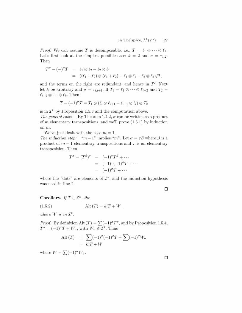
Proof. We can assume T is decomposable, i.e., T = ℓ1 ⊗ · · · ⊗ ℓk.Let’s first look at the simplest possible case: k = 2 and σ = τ1,2.Then

T σ − (−)σT = ℓ1 ⊗ ℓ2 + ℓ2 ⊗ ℓ1

= ((ℓ1 + ℓ2) ⊗ (ℓ1 + ℓ2) − ℓ1 ⊗ ℓ1 − ℓ2 ⊗ ℓ2)/2 ,

and the terms on the right are redundant, and hence in I2. Nextlet k be arbitrary and σ = τi,i+1. If T1 = ℓ1 ⊗ · · · ⊗ ℓi−2 and T2 =ℓi+2 ⊗ · · · ⊗ ℓk. Then

T − (−1)σT = T1 ⊗ (ℓi ⊗ ℓi+1 + ℓi+1 ⊗ ℓi) ⊗ T2

is in Ik by Proposition 1.5.3 and the computation above.The general case: By Theorem 1.4.2, σ can be written as a productof m elementary transpositions, and we’ll prove (1.5.1) by inductionon m.

We’ve just dealt with the case m = 1.The induction step: “m− 1” implies “m”. Let σ = τβ where β is aproduct of m− 1 elementary transpositions and τ is an elementarytransposition. Then

T σ = (T β)τ = (−1)τT β + · · ·

= (−1)τ (−1)βT + · · ·

= (−1)σT + · · ·

where the “dots” are elements of Ik, and the induction hypothesiswas used in line 2.

Corollary. If T ∈ Lk, the

(1.5.2) Alt (T ) = k!T +W ,

where W is in Ik.

Proof. By definition Alt (T ) =∑

(−1)σT σ, and by Proposition 1.5.4,T σ = (−1)σT +Wσ, with Wσ ∈ Ik. Thus

Alt (T ) =∑

(−1)σ(−1)σT +∑

(−1)σWσ

= k!T +W

where W =∑

(−1)σWσ.


Corollary. Ik is the kernel of Alt .

Proof. We’ve already proved that if T ∈ Ik, Alt (T ) = 0. To provethe converse assertion we note that if Alt (T ) = 0, then by (1.5.2)

T = − 1k!W .

with W ∈ Ik .

Putting these results together we conclude:

Theorem 1.5.5. Every element, T , of Lk can be written uniquelyas a sum, T = T1 + T2 where T1 ∈ Ak and T2 ∈ Ik.

Proof. By (1.5.2), T = T1 + T2 with

T1 = 1k!Alt (T )

and

T2 = − 1k!W .

To prove that this decomposition is unique, suppose T1 + T2 = 0,with T1 ∈ Ak and T2 ∈ Ik. Then

0 = Alt (T1 + T2) = k!T1

so T1 = 0, and hence T2 = 0.

Let

(1.5.3) Λk(V ∗) = Lk(V ∗)/Ik(V ∗) ,

i.e., let Λk = Λk(V ∗) be the quotient of the vector space Lk by thesubspace, Ik, of Lk. By (1.2.3) one has a linear map:

(1.5.4) π : Lk → Λk , T → T + Ik

which is onto and has Ik as kernel. We claim:

Theorem 1.5.6. The map, π, maps Ak bijectively onto Λk.

Proof. By Theorem 1.5.5 every Ik coset, T + Ik, contains a uniqueelement, T1, of Ak. Hence for every element of Λk there is a uniqueelement of Ak which gets mapped onto it by π.

1.5 The space, Λk(V ∗) 29

Remark. Since Λk and Ak are isomorphic as vector spaces manytreatments of multilinear algebra avoid mentioning Λk, reasoningthat Ak is a perfectly good substitute for it and that one should,if possible, not make two different definitions for what is essentiallythe same object. This is a justifiable point of view (and is the pointof view taken by Spivak and Munkres1). There are, however, someadvantages to distinguishing between Ak and Λk, as we’ll see in § 1.6.

Exercises.

1. A k-tensor, T , ∈ Lk(V ) is symmetric if T σ = T for all σ ∈ Sk.Show that the set, Sk(V ), of symmetric k tensors is a vector subspaceof Lk(V ).

2. Let e1, . . . , en be a basis of V . Show that every symmetric 2-tensor is of the form ∑

aije∗i ⊗ e∗j

where ai,j = aj,i and e∗1, . . . , e∗n are the dual basis vectors of V ∗.

3. Show that if T is a symmetric k-tensor, then for k ≥ 2, T isin Ik. Hint: Let σ be a transposition and deduce from the identity,T σ = T , that T has to be in the kernel of Alt .

4. Warning: In general Sk(V ) 6= Ik(V ). Show, however, that ifk = 2 these two spaces are equal.

5. Show that if ℓ ∈ V ∗ and T ∈ Ik−2, then ℓ⊗ T ⊗ ℓ is in Ik.

6. Show that if ℓ1 and ℓ2 are in V ∗ and T is in Ik−2, then ℓ1 ⊗T ⊗ ℓ2 + ℓ2 ⊗ T ⊗ ℓ1 is in Ik.

7. Given a permutation σ ∈ Sk and T ∈ Ik, show that T σ ∈ Ik.

8. Let W be a subspace of Lk having the following two properties.

(a) For S ∈ S2(V ) and T ∈ Lk−2, S ⊗ T is in W.

(b) For T in W and σ ∈ Sk, Tσ is in W.

1and by the author of these notes in his book with Alan Pollack, “Differential Topol-ogy”


Show that W has to contain Ik and conclude that Ik is the small-est subspace of Lk having properties a and b.

9. Show that there is a bijective linear map

α : Λk → Ak

with the property

(1.5.5) απ(T ) =1

k!Alt (T )

for all T ∈ Lk, and show that α is the inverse of the map of Ak ontoΛk described in Theorem 1.5.6 (Hint: §1.2, exercise 8).

10. Let V be an n-dimensional vector space. Compute the dimen-sion of Sk(V ). Some hints:

(a) Introduce the following symmetrization operation on tensorsT ∈ Lk(V ):

Sym(T ) =∑

τ∈Sk

T τ .

Prove that this operation has properties 2, 3 and 4 of Proposi-tion 1.4.6 and, as a substitute for property 1, has the property:(SymT )σ = SymT .

(b) Let ϕI = Sym(e∗I), e∗I = e∗i1 ⊗ · · · ⊗ e∗in . Prove that ϕI , I

non-decreasing form a basis of Sk(V ).

(c) Conclude from (b) that dimSk(V ) is equal to the number ofnon-decreasing multi-indices of length k: 1 ≤ i1 ≤ i2 ≤ · · · ≤ ℓk ≤ n.

(d) Compute this number by noticing that

(i1, . . . , in) → (i1 + 0, i2 + 1, . . . , ik + k − 1)

is a bijection between the set of these non-decreasing multi-indicesand the set of increasing multi-indices 1 ≤ j1 < · · · < jk ≤ n+ k− 1.

1.6 The wedge product 31

1.6 The wedge product

The tensor algebra operations on the spaces, Lk(V ), which we dis-cussed in Sections 1.2 and 1.3, i.e., the “tensor product operation”and the “pull-back” operation, give rise to similar operations on thespaces, Λk. We will discuss in this section the analogue of the tensorproduct operation. As in § 4 we’ll abbreviate Lk(V ) to Lk and Λk(V )to Λk when it’s clear which “V ” is intended.

Given ωi ∈ Λki , i = 1, 2 we can, by (1.5.4), find a Ti ∈ Lki withωi = π(Ti). Then T1 ⊗ T2 ∈ Lk1+k2 . Let

(1.6.1) ω1 ∧ ω2 = π(T1 ⊗ T2) ∈ Λk1+k2 .

Claim.

This wedge product is well defined, i.e., doesn’t depend on our choicesof T1 and T2.

Proof. Let π(T1) = π(T ′1) = ω1. Then T ′

1 = T1 +W1 for some W1 ∈Ik1, so

T ′1 ⊗ T2 = T1 ⊗ T2 +W1 ⊗ T2 .

But W1 ∈ Ik1 implies W1 ⊗ T2 ∈ Ik1+k2 and this implies:

π(T ′1 ⊗ T2) = π(T1 ⊗ T2) .

A similar argument shows that (1.6.1) is well-defined independent ofthe choice of T2.

More generally let ωi ∈ Λki , i = 1, 2, 3, and let ωi = π(Ti), Ti ∈Lki . Define

ω1 ∧ ω2 ∧ ω3 ∈ Λk1+k2+k3

by settingω1 ∧ ω2 ∧ ω3 = π(T1 ⊗ T2 ⊗ T3) .

As above it’s easy to see that this is well-defined independent of thechoice of T1, T2 and T3. It is also easy to see that this triple wedgeproduct is just the wedge product of ω1∧ω2 with ω3 or, alternatively,the wedge product of ω1 with ω2 ∧ ω3, i.e.,

(1.6.2) ω1 ∧ ω2 ∧ ω3 = (ω1 ∧ ω2) ∧ ω3 = ω1 ∧ (ω2 ∧ ω3).


We leave for you to check:For λ ∈ R

(1.6.3) λ(ω1 ∧ ω2) = (λω1) ∧ ω2 = ω1 ∧ (λω2)

and verify the two distributive laws:

(ω1 + ω2) ∧ ω3 = ω1 ∧ ω3 + ω2 ∧ ω3(1.6.4)

and

ω1 ∧ (ω2 + ω3) = ω1 ∧ ω2 + ω1 ∧ ω3 .(1.6.5)

As we noted in § 1.4, Ik = 0 for k = 1, i.e., there are no non-zero“redundant” k tensors in degree k = 1. Thus

(1.6.6) Λ1(V ∗) = V ∗ = L1(V ∗).

A particularly interesting example of a wedge product is the fol-lowing. Let ℓi ∈ V ∗ = Λ1(V ∗), i = 1, . . . , k. Then if T = ℓ1 ⊗ · · · ⊗ ℓk

(1.6.7) ℓ1 ∧ · · · ∧ ℓk = π(T ) ∈ Λk(V ∗) .

We will call (1.6.7) a decomposable element of Λk(V ∗).We will prove that these elements satisfy the following wedge prod-

uct identity. For σ ∈ Sk:

(1.6.8) ℓσ(1) ∧ · · · ∧ ℓσ(k) = (−1)σℓ1 ∧ · · · ∧ ℓk .

Proof. For every T ∈ Lk, T = (−1)σT + W for some W ∈ Ik byProposition 1.5.4. Therefore since π(W ) = 0

(1.6.9) π(T σ) = (−1)σπ(T ) .

In particular, if T = ℓ1 ⊗ · · · ⊗ ℓk, Tσ = ℓσ(1) ⊗ · · · ⊗ ℓσ(k), so

π(T σ) = ℓσ(1) ∧ · · · ∧ ℓσ(k) = (−1)σπ(T )

= (−1)σℓ1 ∧ · · · ∧ ℓk .

In particular, for ℓ1 and ℓ2 ∈ V ∗

(1.6.10) ℓ1 ∧ ℓ2 = −ℓ2 ∧ ℓ1

1.6 The wedge product 33

and for ℓ1, ℓ2 and ℓ3 ∈ V ∗

(1.6.11) ℓ1 ∧ ℓ2 ∧ ℓ3 = −ℓ2 ∧ ℓ1 ∧ ℓ3 = ℓ2 ∧ ℓ3 ∧ ℓ1 .

More generally, it’s easy to deduce from (1.6.8) the following result(which we’ll leave as an exercise).

Theorem 1.6.1. If ω1 ∈ Λr and ω2 ∈ Λs then

(1.6.12) ω1 ∧ ω2 = (−1)rsω2 ∧ ω1 .

Hint: It suffices to prove this for decomposable elements i.e., forω1 = ℓ1 ∧ · · · ∧ ℓr and ω2 = ℓ′1 ∧ · · · ∧ ℓ′s. Now make rs applicationsof (1.6.10).

Let e1, . . . , en be a basis of V and let e∗1, . . . , e∗n be the dual basis

of V ∗. For every multi-index, I, of length k,

(1.6.13) e∗i1 ∧ · · · e∗ik = π(e∗I) = π(e∗i1 ⊗ · · · ⊗ e∗ik) .

Theorem 1.6.2. The elements (1.6.13), with I strictly increasing,are basis vectors of Λk.

Proof. The elements

ψI = Alt (e∗I) , I strictly increasing,

are basis vectors of Ak by Proposition 3.6; so their images, π(ψI),are a basis of Λk. But

π(ψI) = π∑

(−1)σ(e∗I)σ

=∑

(−1)σπ(e∗I)σ

=∑

(−1)σ(−1)σπ(e∗I)

= k!π(e∗I) .

Exercises:

1. Prove the assertions (1.6.3), (1.6.4) and (1.6.5).

2. Verify the multiplication law, (1.6.12) for wedge product.


3. Given ω ∈ Λr let ωk be the k-fold wedge product of ω withitself, i.e., let ω2 = ω ∧ ω, ω3 = ω ∧ ω ∧ ω, etc.

(a) Show that if r is odd then for k > 1, ωk = 0.

(b) Show that if ω is decomposable, then for k > 1, ωk = 0.

4. If ω and µ are in Λ2r prove:

(ω + µ)k =

k∑

ℓ=0

(k

ℓ

)ωℓ ∧ µk−ℓ .

Hint: As in freshman calculus prove this binomial theorem by induc-tion using the identity:

(kℓ

)=(k−1ℓ−1

)+(k−1

ℓ

).

5. Let ω be an element of Λ2. By definition the rank of ω is k ifωk 6= 0 and ωk+1 = 0. Show that if

ω = e1 ∧ f1 + · · · + ek ∧ fk

with ei, fi ∈ V ∗, then ω is of rank ≤ k. Hint: Show that

ωk = k!e1 ∧ f1 ∧ · · · ∧ ek ∧ fk .

6. Given ei ∈ V ∗, i = 1, . . . , k show that e1 ∧ · · · ∧ ek 6= 0 if andonly if the ei’s are linearly independent. Hint: Induction on k.

1.7 The interior product 35

1.7 The interior product

We’ll describe in this section another basic product operation on thespaces, Λk(V ∗). As above we’ll begin by defining this operator onthe Lk(V )’s. Given T ∈ Lk(V ) and v ∈ V let ιvT be the be the(k − 1)-tensor which takes the value(1.7.1)

ιvT (v1, . . . , vk−1) =

k∑

r=1

(−1)r−1T (v1, . . . , vr−1, v, vr, . . . , vk−1)

on the k − 1-tuple of vectors, v1, . . . , vk−1, i.e., in the rth summandon the right, v gets inserted between vr−1 and vr. (In particularthe first summand is T (v, v1, . . . , vk−1) and the last summand is(−1)k−1T (v1, . . . , vk−1, v).) It’s clear from the definition that if v =v1 + v2

ιvT = ιv1T + ιv2

T ,(1.7.2)

and if T = T1 + T2

ιvT = ιvT1 + ιvT2 ,(1.7.3)

and we will leave for you to verify by inspection the following twolemmas:

Lemma 1.7.1. If T is the decomposable k-tensor ℓ1 ⊗ · · · ⊗ ℓk then

(1.7.4) ιvT =∑

(−1)r−1ℓr(v)ℓ1 ⊗ · · · ⊗ ℓr ⊗ · · · ⊗ ℓk

where the “cap” over ℓr means that it’s deleted from the tensor prod-uct ,

and

Lemma 1.7.2. If T1 ∈ Lp and T2 ∈ Lq

(1.7.5) ιv(T1 ⊗ T2) = ιvT1 ⊗ T2 + (−1)pT1 ⊗ ιvT2 .

We will next prove the important identity

(1.7.6) ιv(ιvT ) = 0 .

Proof. It suffices by linearity to prove this for decomposable tensorsand since (1.7.6) is trivially true for T ∈ L1, we can by induction


assume (1.7.6) is true for decomposible tensors of degree k − 1. Letℓ1 ⊗ · · · ⊗ ℓk be a decomposable tensor of degree k. Setting T =ℓ1 ⊗ · · · ⊗ ℓk−1 and ℓ = ℓk we have

ιv(ℓ1 ⊗ · · · ⊗ ℓk) = ιv(T ⊗ ℓ)

= ιvT ⊗ ℓ+ (−1)k−1ℓ(v)T

by (1.7.5). Hence

ιv(ιv(T ⊗ ℓ)) = ιv(ιvT ) ⊗ ℓ+ (−1)k−2ℓ(v)ιvT

+(−1)k−1ℓ(v)ιvT .

But by induction the first summand on the right is zero and the tworemaining summands cancel each other out.

From (1.7.6) we can deduce a slightly stronger result: For v1, v2 ∈V

(1.7.7) ιv1ιv2

= −ιv2ιv1

.

Proof. Let v = v1 + v2. Then ιv = ιv1+ ιv2

so

0 = ιvιv = (ιv1+ ιv2

)(ιv1+ ιv2

)

= ιv1ιv1

+ ιv1ιv2

+ ιv2ιv1

+ ιv2ιv2

= ιv1ιv2

+ ιv2ιv1

since the first and last summands are zero by (1.7.6).

We’ll now show how to define the operation, ιv, on Λk(V ∗). We’llfirst prove

Lemma 1.7.3. If T ∈ Lk is redundant then so is ιvT .

Proof. Let T = T1 ⊗ ℓ⊗ ℓ⊗ T2 where ℓ is in V ∗, T1 is in Lp and T2

is in Lq. Then by (1.7.5)

ιvT = ιvT1 ⊗ ℓ⊗ ℓ⊗ T2

+(−1)pT1 ⊗ ιv(ℓ⊗ ℓ) ⊗ T2

+(−1)p+2T1 ⊗ ℓ⊗ ℓ⊗ ιvT2 .

1.7 The interior product 37

However, the first and the third terms on the right are redundantand

ιv(ℓ⊗ ℓ) = ℓ(v)ℓ− ℓ(v)ℓ

by (1.7.4).

Now let π be the projection (1.5.4) of Lk onto Λk and for ω =π(T ) ∈ Λk define

(1.7.8) ιvω = π(ιvT ) .

To show that this definition is legitimate we note that if ω = π(T1) =π(T2), then T1 −T2 ∈ Ik, so by Lemma 1.7.3 ιvT1 − ιvT2 ∈ Ik−1 andhence

π(ιvT1) = π(ιvT2) .

Therefore, (1.7.8) doesn’t depend on the choice of T .By definition ιv is a linear mapping of Λk(V ∗) into Λk−1(V ∗).

We will call this the interior product operation. From the identities(1.7.2)–(1.7.8) one gets, for v, v1, v2 ∈ V ω ∈ Λk, ω1 ∈ Λp andω2 ∈ Λ2

ι(v1+v2)ω = ιv1ω + ιv2

ω(1.7.9)

ιv(ω1 ∧ ω2) = ιvω1 ∧ ω2 + (−1)pω1 ∧ ιvω2(1.7.10)

ιv(ιvω) = 0(1.7.11)

and

ιv1ιv2ω = −ιv2

ιv1ω .(1.7.12)

Moreover if ω = ℓ1 ∧ · · · ∧ ℓk is a decomposable element of Λk onegets from (1.7.4)

(1.7.13) ιvω =k∑

r=1

(−1)r−1ℓr(v)ℓ1 ∧ · · · ∧ ℓr ∧ · · · ∧ ℓk .

In particular if e1, . . . , en is a basis of V , e∗1, . . . , e∗n the dual basis of

V ∗ and ωI = e∗i1 ∧ · · · ∧ e∗ik , 1 ≤ i1 < · · · < ik ≤ n, then ι(ej)ωI = 0if j /∈ I and if j = ir

(1.7.14) ι(ej)ωI = (−1)r−1ωIr

where Ir = (i1, . . . , ir, . . . , ik) (i.e., Ir is obtained from the multi-index I by deleting ir).


Exercises:

1. Prove Lemma 1.7.1.

2. Prove Lemma 1.7.2.

3. Show that if T ∈ Ak, iv = kTv where Tv is the tensor (1.3.16).In particular conclude that ivT ∈ Ak−1. (See §1.4, exercise 8.)

4. Assume the dimension of V is n and let Ω be a non-zero elementof the one dimensional vector space Λn. Show that the map

(1.7.15) ρ : V → Λn−1 , v → ιvΩ ,

is a bijective linear map. Hint: One can assume Ω = e∗1 ∧ · · · ∧ e∗nwhere e1, . . . , en is a basis of V . Now use (1.7.14) to compute thismap on basis elements.

5. (The cross-product.) Let V be a 3-dimensional vector space, Ban inner product on V and Ω a non-zero element of Λ3. Define a map

V × V → V

by setting

(1.7.16) v1 × v2 = ρ−1(Lv1 ∧ Lv2)

where ρ is the map (1.7.15) and L : V → V ∗ the map (1.2.9). Showthat this map is linear in v1, with v2 fixed and linear in v2 with v1fixed, and show that v1 × v2 = −v2 × v1.

6. For V = R3 let e1, e2 and e3 be the standard basis vectors and

B the standard inner product. (See §1.1.) Show that if Ω = e∗1∧e∗2∧e

∗3

the cross-product above is the standard cross-product:

e1 × e2 = e3

e2 × e3 = e1(1.7.17)

e3 × e1 = e2 .

Hint: If B is the standard inner product Lei = e∗i .

Remark 1.7.4. One can make this standard cross-product look evenmore standard by using the calculus notation: e1 = i, e2 = j ande3 = k

1.8 The pull-back operation on Λk 39

1.8 The pull-back operation on Λk

Let V and W be vector spaces and let A be a linear map of V intoW . Given a k-tensor, T ∈ Lk(W ), the pull-back, A∗T , is the k-tensor

(1.8.1) A∗T (v1, . . . , vk) = T (Av1, . . . , Avk)

in Lk(V ). (See § 1.3, equation 1.3.12.) In this section we’ll show howto define a similar pull-back operation on Λk.

Lemma 1.8.1. If T ∈ Ik(W ), then A∗T ∈ Ik(V ).

Proof. It suffices to verify this when T is a redundant k-tensor, i.e., atensor of the form

T = ℓ1 ⊗ · · · ⊗ ℓk

where ℓr ∈W ∗ and ℓi = ℓi+1 for some index, i. But by (1.3.14)

A∗T = A∗ℓ1 ⊗ · · · ⊗A∗ℓk

and the tensor on the right is redundant since A∗ℓi = A∗ℓi+1.

Now let ω be an element of Λk(W ∗) and let ω = π(T ) where T isin Lk(W ). We define

(1.8.2) A∗ω = π(A∗T ) .

Claim:

The left hand side of (1.8.2) is well-defined.

Proof. If ω = π(T ) = π(T ′), then T = T ′ + S for some S ∈ Ik(W ),and A∗T ′ = A∗T +A∗S. But A∗S ∈ Ik(V ), so

π(A∗T ′) = π(A∗T ) .

Proposition 1.8.2. The map

A∗ : Λk(W ∗) → Λk(V ∗) ,

mapping ω to A∗ω is linear. Moreover,


(i) If ωi ∈ Λki(W ), i = 1, 2, then

(1.8.3) A∗(ω1 ∧ ω2) = A∗ω1 ∧A∗ω2 .

(ii) If U is a vector space and B : U → V a linear map, thenfor ω ∈ Λk(W ∗),

(1.8.4) B∗A∗ω = (AB)∗ω .

We’ll leave the proof of these three assertions as exercises. Hint:They follow immediately from the analogous assertions for the pull-back operation on tensors. (See (1.3.14) and (1.3.15).)

As an application of the pull-back operation we’ll show how touse it to define the notion of determinant for a linear mapping. LetV be a n-dimensional vector space. Then dim Λn(V ∗) =

(nn

)= 1;

i.e., Λn(V ∗) is a one-dimensional vector space. Thus if A : V → Vis a linear mapping, the induced pull-back mapping:

A∗ : Λn(V ∗) → Λn(V ∗) ,

is just “multiplication by a constant”. We denote this constant bydet(A) and call it the determinant of A, Hence, by definition,

(1.8.5) A∗ω = det(A)ω

for all ω in Λn(V ∗). From (1.8.5) it’s easy to derive a number of basicfacts about determinants.

Proposition 1.8.3. If A and B are linear mappings of V into V ,then

(1.8.6) det(AB) = det(A) det(B) .

Proof. By (1.8.4) and

(AB)∗ω = det(AB)ω

= B∗(A∗ω) = det(B)A∗ω

= det(B) det(A)ω ,

so, det(AB) = det(A) det(B).


Proposition 1.8.4. If I : V → V is the identity map, Iv = v forall v ∈ V , det(I) = 1.

We’ll leave the proof as an exercise. Hint: I∗ is the identity mapon Λn(V ∗).

Proposition 1.8.5. If A : V → V is not onto, det(A) = 0.

Proof. LetW be the image of A. Then if A is not onto, the dimensionof W is less than n, so Λn(W ∗) = 0. Now let A = IWB where IWis the inclusion map of W into V and B is the mapping, A, regardedas a mapping from V to W . Thus if ω is in Λn(V ∗), then by (1.8.4)

A∗ω = B∗I∗Wω

and since I∗Wω is in Λn(W ) it is zero.

We will derive by wedge product arguments the familiar “matrixformula” for the determinant. Let V and W be n-dimensional vectorspaces and let e1, . . . , en be a basis for V and f1, . . . , fn a basis forW . From these bases we get dual bases, e∗1, . . . , e

∗n and f∗1 , . . . , f

∗n,

for V ∗ and W ∗. Moreover, if A is a linear map of V into W and[ai,j] the n×n matrix describing A in terms of these bases, then thetranspose map, A∗ : W ∗ → V ∗, is described in terms of these dualbases by the n× n transpose matrix, i.e., if

Aej =∑

ai,jfi ,

then

A∗f∗j =∑

aj,ie∗i .

(See § 2.) Consider now A∗(f∗1 ∧ · · · ∧ f∗n). By (1.8.3)

A∗(f∗1 ∧ · · · ∧ f∗n) = A∗f∗1 ∧ · · · ∧A∗f∗n

=∑

(a1,k1e∗k1

) ∧ · · · ∧ (an,kne∗kn

)

the sum being over all k1, . . . , kn, with 1 ≤ kr ≤ n. Thus,

A∗(f∗1 ∧ · · · ∧ f∗n) =∑

a1,k1. . . an,kn

e∗k1∧ · · · ∧ e∗kn

.


If the multi-index, k1, . . . , kn, is repeating, then e∗k1∧· · ·∧e∗kn

is zero,and if it’s not repeating then we can write

ki = σ(i) i = 1, . . . , n

for some permutation, σ, and hence we can rewrite A∗(f∗1 ∧ · · · ∧ f∗n)as the sum over σ ∈ Sn of

∑a1,σ(1) · · · an,σ(n) (e∗1 ∧ · · · ∧ e∗n)σ .

But(e∗1 ∧ · · · ∧ e∗n)σ = (−1)σe∗1 ∧ · · · ∧ e∗n

so we get finally the formula

(1.8.7) A∗(f∗1 ∧ · · · ∧ f∗n) = det[ai,j]e∗1 ∧ · · · ∧ e∗n

where

(1.8.8) det[ai,j ] =∑

(−1)σa1,σ(1) · · · an,σ(n)

summed over σ ∈ Sn. The sum on the right is (as most of you know)the determinant of [ai,j].

Notice that if V = W and ei = fi, i = 1, . . . , n, then ω = e∗1∧· · ·∧e∗n = f∗1 ∧ · · · ∧ f∗n, hence by (1.8.5) and (1.8.7),

(1.8.9) det(A) = det[ai,j] .

Exercises.

1. Verify the three assertions of Proposition 1.8.2.

2. Deduce from Proposition 1.8.5 a well-known fact about deter-minants of n×n matrices: If two columns are equal, the determinantis zero.

3. Deduce from Proposition 1.8.3 another well-known fact aboutdeterminants of n × n matrices: If one interchanges two columns,then one changes the sign of the determinant.

Hint: Let e1, . . . , en be a basis of V and let B : V → V be thelinear mapping: Bei = ej, Bej = ei and Beℓ = eℓ, ℓ 6= i, j. What isB∗(e∗1 ∧ · · · ∧ e∗n)?


4. Deduce from Propositions 1.8.3 and 1.8.4 another well-knownfact about determinants of n × n matrix. If [bi,j ] is the inverse of[ai,j], its determinant is the inverse of the determinant of [ai,j ].

5. Extract from (1.8.8) a well-known formula for determinants of2 × 2 matrices:

det

[a11 , a12

a21 , a22

]= a11a22 − a12a21 .

6. Show that if A = [ai,j ] is an n× n matrix and At = [aj,i] is itstranspose detA = detAt. Hint: You are required to show that thesums

∑(−1)σa1,σ(1) . . . an,σ(n) σ ∈ Sn

and

∑(−1)σaσ(1),1 . . . aσ(n),n σ ∈ Sn

are the same. Show that the second sum is identical with∑

(−1)τaτ(1),1 . . . aτ(n),n

summed over τ = σ−1 ∈ Sn.

7. Let A be an n× n matrix of the form

A =

[B ∗0 C

]

where B is a k × k matrix and C the ℓ × ℓ matrix and the bottomℓ× k block is zero. Show that

detA = detB detC .

Hint: Show that in (1.8.8) every non-zero term is of the form

(−1)στ b1,σ(1) . . . bk,σ(k)c1,τ(1) . . . cℓ,τ(ℓ)

where σ ∈ Sk and τ ∈ Sℓ.

8. Let V and W be vector spaces and let A : V → W be a linearmap. Show that if Av = w then for ω ∈ Λp(w∗),

A∗ι(w)ω = ι(v)A∗ω .

(Hint: By (1.7.10) and proposition 1.8.2 it suffices to prove this forω ∈ Λ1(W ∗), i.e., for ω ∈W ∗.)


1.9 Orientations

We recall from freshman calculus that if ℓ ⊆ R2 is a line through the

origin, then ℓ−0 has two connected components and an orientationof ℓ is a choice of one of these components (as in the figure below).

• 0

ℓ

More generally, if L is a one-dimensional vector space then L−0consists of two components: namely if v is an element of L− [0, thenthese two components are

L1 = λv λ > 0

and

L2 = λv, λ < 0 .

An orientation of L is a choice of one of these components. Usu-ally the component chosen is denoted L+, and called the positivecomponent of L − 0 and the other component, L−, the negativecomponent of L − 0.

Definition 1.9.1. A vector, v ∈ L, is positively oriented if v is inL+.

More generally still let V be an n-dimensional vector space. ThenL = Λn(V ∗) is one-dimensional, and we define an orientation of Vto be an orientation of L. One important way of assigning an orien-tation to V is to choose a basis, e1, . . . , en of V . Then, if e∗1, . . . , e

∗n is

the dual basis, we can orient Λn(V ∗) by requiring that e∗1∧· · ·∧e∗n bein the positive component of Λn(V ∗). If V has already been assignedan orientation we will say that the basis, e1, . . . , en, is positively ori-ented if the orientation we just described coincides with the givenorientation.

Suppose that e1, . . . , en and f1, . . . , fn are bases of V and that

(1.9.1) ej =∑

ai,j,fi .

1.9 Orientations 45

Then by (1.7.7)

f∗1 ∧ · · · ∧ f∗n = det[ai,j ]e∗1 ∧ · · · ∧ e∗n

so we conclude:

Proposition 1.9.2. If e1, . . . , en is positively oriented, then f1, . . . , fn

is positively oriented if and only if det[ai,j ] is positive.

Corollary 1.9.3. If e1, . . . , en is a positively oriented basis of V , thebasis: e1, . . . , ei−1,−ei, ei+1, . . . , en is negatively oriented.

Now let V be a vector space of dimension n > 1 and W a sub-space of dimension k < n. We will use the result above to prove thefollowing important theorem.

Theorem 1.9.4. Given orientations on V and V/W , one gets fromthese orientations a natural orientation on W .

Remark What we mean by “natural’ will be explained in the courseof the proof.

Proof. Let r = n − k and let π be the projection of V onto V/W. By exercises 1 and 2 of §2 we can choose a basis e1, . . . , en of Vsuch that er+1, . . . , en is a basis of W and π(e1), . . . , π(er) a basisof V/W . Moreover, replacing e1 by −e1 if necessary we can assumeby Corollary 1.9.3 that π(e1), . . . , π(er) is a positively oriented basisof V/W and replacing en by −en if necessary we can assume thate1, . . . , en is a positively oriented basis of V . Now assign to W theorientation associated with the basis er+1, . . . , en.

Let’s show that this assignment is “natural” (i.e., doesn’t dependon our choice of e1, . . . , en). To see this let f1, . . . , fn be anotherbasis of V with the properties above and let A = [ai,j ] be the matrix(1.9.1) expressing the vectors e1, . . . , en as linear combinations of thevectors f1, . . . fn. This matrix has to have the form

(1.9.2) A =

[B C0 D

]

whereB is the r×rmatrix expressing the basis vectors π(e1), . . . , π(er)of V/W as linear combinations of π(f1), . . . , π(fr) and D the k × kmatrix expressing the basis vectors er+1, . . . , en of W as linear com-binations of fr+1, . . . , fn. Thus

det(A) = det(B) det(D) .


However, by Proposition 1.9.2, detA and detB are positive, so detDis positive, and hence if er+1, . . . , en is a positively oriented basis ofW so is fr+1, . . . , fn.

As a special case of this theorem suppose dimW = n − 1. Thenthe choice of a vector v ∈ V − W gives one a basis vector, π(v),for the one-dimensional space V/W and hence if V is oriented, thechoice of v gives one a natural orientation on W .

Next let Vi, i = 1, 2 be oriented n-dimensional vector spaces andA : V1 → V2 a bijective linear map. A is orientation-preserving if,for ω ∈ Λn(V ∗

2 )+, A∗ω is in Λn(V ∗+)+. For example if V1 = V2 then

A∗ω = det(A)ω so A is orientation preserving if and only if det(A) >0. The following proposition we’ll leave as an exercise.

Proposition 1.9.5. Let Vi, i = 1, 2, 3 be oriented n-dimensionalvector spaces and Ai : Vi → Vi+1, i = 1, 2 bijective linear maps.Then if A1 and A2 are orientation preserving, so is A2 A1.

Exercises.

1. Prove Corollary 1.9.3.

2. Show that the argument in the proof of Theorem 1.9.4 can bemodified to prove that if V and W are oriented then these orienta-tions induce a natural orientation on V/W .

3. Similarly show that if W and V/W are oriented these orienta-tions induce a natural orientation on V .

4. Let V be an n-dimensional vector space and W ⊂ V a k-dimensional subspace. Let U = V/W and let ι : W → V andπ : V → U be the inclusion and projection maps. Suppose V and Uare oriented. Let µ be in Λn−k(U∗)+ and let ω be in Λn(V ∗)+. Showthat there exists a ν in Λk(V ∗) such that π∗µ ∧ ν = ω. Moreovershow that ι∗ν is intrinsically defined (i.e., doesn’t depend on howwe choose ν) and sits in the positive part, Λk(W ∗)+, of Λk(W ).

5. Let e1, . . . , en be the standard basis vectors of Rn. The standard

orientation of Rn is, by definition, the orientation associated with

this basis. Show that if W is the subspace of Rn defined by the

1.9 Orientations 47

equation, x1 = 0, and v = e1 6∈W then the natural orientation of Wassociated with v and the standard orientation of R

n coincide withthe orientation given by the basis vectors, e2, . . . , en of W .

6. Let V be an oriented n-dimensional vector space and W ann−1-dimensional subspace. Show that if v and v′ are in V −W thenv′ = λv + w, where w is in W and λ ∈ R − 0. Show that v and v′

give rise to the same orientation of W if and only if λ is positive.

7. Prove Proposition 1.9.5.

8. A key step in the proof of Theorem 1.9.4 was the assertion thatthe matrix A expressing the vectors, ei, as linear combinations of thevectors, fi, had to have the form (1.9.2). Why is this the case?

9. (a) Let V be a vector space, W a subspace of V and A : V →V a bijective linear map which maps W onto W . Show that one getsfrom A a bijective linear map

B : V/W → V/W

with property

πA = Bπ ,

π being the projection of V onto V/W .

(b) Assume that V , W and V/W are compatibly oriented. Showthat if A is orientation-preserving and its restriction to W is orien-tation preserving then B is orientation preserving.

10. Let V be a oriented n-dimensional vector space, W an (n− 1)-dimensional subspace of V and i : W → V the inclusion map. Givenω ∈ Λb(V )+ and v ∈ V − W show that for the orientation of Wdescribed in exercise 5, i∗(ιvω) ∈ Λn−1(W )+.

11. Let V be an n-dimensional vector space, B : V × V → R aninner product and e1, . . . , en a basis of V which is positively orientedand orthonormal. Show that the “volume element”

vol = e∗1 ∧ · · · ∧ e∗n ∈ Λn(V ∗)

is intrinsically defined, independent of the choice of this basis. Hint:(1.2.13) and (1.8.7).


12. (a) Let V be an oriented n-dimensional vector space and B aninner product on V . Fix an oriented orthonormal basis, e1, . . . , en,of V and let A : V → V be a linear map. Show that if

Aei = vi =∑

aj,iej

and bi,j = B(vi, vj), the matrices A = [ai,j ] and B = [bi,j] are relatedby: B = A+A.

(b) Show that if ν is the volume form, e∗1 ∧ · · · ∧ e∗n, and A is orien-tation preserving

A∗ν = (detB)1

2 ν .

(c) By Theorem 1.5.6 one has a bijective map

Λn(V ∗) ∼= An(V ) .

Show that the element, Ω, of An(V ) corresponding to the form, ν,has the property

|Ω(v1, . . . , vn)|2 = det([bi,j ])

where v1, . . . , vn are any n-tuple of vectors in V and bi,j = B(vi, vj).


CHAPTER 2

DIFFERENTIAL FORMS

2.1 Vector fields and one-forms

The goal of this chapter is to generalize to n dimensions the basicoperations of three dimensional vector calculus: div, curl and grad.The “div”, and “grad” operations have fairly straight forward gener-alizations, but the “curl” operation is more subtle. For vector fieldsit doesn’t have any obvious generalization, however, if one replacesvector fields by a closely related class of objects, differential forms,then not only does it have a natural generalization but it turns outthat div, curl and grad are all special cases of a general operation ondifferential forms called exterior differentiation.

In this section we will review some basic facts about vector fieldsin n variables and introduce their dual objects: one-forms. We willthen take up in §2.2 the theory of k-forms for k greater than one.We begin by fixing some notation.

Given p ∈ Rn we define the tangent space to R

n at p to be the setof pairs

(2.1.1) TpRn = (p, v) ; v ∈ R

n .

The identification

(2.1.2) TpRn → R

n , (p, v) → v

makes TpRn into a vector space. More explicitly, for v, v1 and v2 ∈ R

n

and λ ∈ R we define the addition and scalar multiplication operationson TpR

n by the recipes

(p, v1) + (p, v2) = (p, v1 + v2)

and

λ(p, v) = (p, λv) .

Let U be an open subset of Rn and f : U → R

m a C1 map. Werecall that the derivative

Df(p) : Rn → R

m

50 Chapter 2. Differential forms

of f at p is the linear map associated with the m× n matrix[∂fi

∂xj(p)

].

It will be useful to have a “base-pointed” version of this definitionas well. Namely, if q = f(p) we will define

dfp : TpRn → TqR

m

to be the map

(2.1.3) dfp(p, v) = (q,Df(p)v) .

It’s clear from the way we’ve defined vector space structures on TpRn

and TqRm that this map is linear.

Suppose that the image of f is contained in an open set, V , andsuppose g : V → R

k is a C1 map. Then the “base-pointed”” versionof the chain rule asserts that

(2.1.4) dgq dfp = d(f g)p .

(This is just an alternative way of writing Dg(q)Df(p) = D(g f)(p).)

In 3-dimensional vector calculus a vector field is a function whichattaches to each point, p, of R

3 a base-pointed arrow, (p,~v). Then-dimensional version of this definition is essentially the same.

Definition 2.1.1. Let U be an open subset of Rn. A vector field on

U is a function, v, which assigns to each point, p, of U a vector v(p)in TpR

n.

Thus a vector field is a vector-valued function, but its value at pis an element of a vector space, TpR

n that itself depends on p.Some examples.

1. Given a fixed vector, v ∈ Rn, the function

(2.1.5) p ∈ Rn → (p, v)

is a vector field. Vector fields of this type are constant vector fields.

2. In particular let ei, i = 1, . . . , n, be the standard basis vectorsof R

n. If v = ei we will denote the vector field (2.1.5) by ∂/∂xi. (Thereason for this “derivation notation” will be explained below.)

2.1 Vector fields and one-forms 51

3. Given a vector field on U and a function, f : U → R we’lldenote by fv the vector field

p ∈ U → f(p)v(p) .

4. Given vector fields v1 and v2 on U , we’ll denote by v1 + v2 thevector field

p ∈ U → v1(p) + v2(p) .

5. The vectors, (p, ei), i = 1, . . . , n, are a basis of TpRn, so if

v is a vector field on U , v(p) can be written uniquely as a linearcombination of these vectors with real numbers, gi(p), i = 1, . . . , n,as coefficients. In other words, using the notation in example 2 above,v can be written uniquely as a sum

(2.1.6) v =

n∑

i=1

gi∂

∂xi

where gi : U → R is the function, p→ gi(p).

We’ll say that v is a C∞ vector field if the gi’s are in C∞(U).A basic vector field operation is Lie differentiation. If f ∈ C1(U)

we define Lvf to be the function on U whose value at p is given by

(2.1.7) Df(p)v = Lvf(p)

where v(p) = (p, v). If v is the vector field (2.1.6) then

(2.1.8) Lvf =∑

gi∂

∂xif

(motivating our “derivation notation” for v).

Exercise.

Check that if fi ∈ C1(U), i = 1, 2, then

(2.1.9) Lv(f1f2) = f1Lvf2 + f1Lvf2 .

Next we’ll generalize to n-variables the calculus notion of an “in-tegral curve” of a vector field.


Definition 2.1.2. A C1 curve γ : (a, b) → U is an integral curve ofv if for all a < t < b and p = γ(t)

(p,dγ

dt(t)

)= v(p)

i.e., if v is the vector field (2.1.6) and g : U → Rn is the function

(g1, . . . , gn) the condition for γ(t) to be an integral curve of v is thatit satisfy the system of differential equations

(2.1.10)dγ

dt(t) = g(γ(t)) .

We will quote without proof a number of basic facts about systemsof ordinary differential equations of the type (2.1.10). (A source forthese results that we highly recommend is Birkhoff–Rota, OrdinaryDifferential Equations, Chapter 6.)

Theorem 2.1.3 (Existence). Given a point p0 ∈ U and a ∈ R, thereexists an interval I = (a− T, a+ T ), a neighborhood, U0, of p0 in Uand for every p ∈ U0 an integral curve, γp : I → U with γp(a) = p.

Theorem 2.1.4 (Uniqueness). Let γi : Ii → U , i = 1, 2, be integralcurves. If a ∈ I1 ∩ I2 and γ1(a) = γ2(a) then γ1 ≡ γ2 on I1 ∩ I2 andthe curve γ : I1 ∪ I2 → U defined by

γ(t) =

γ1(t) , t ∈ I1

γ2(t) , t ∈ I2

is an integral curve.

Theorem 2.1.5 (Smooth dependence on initial data). Let v be aC∞-vector field, on an open subset, V , of U , I ⊆ R an open interval,a ∈ I a point on this interval and h : V × I → U a mapping with theproperties:

(i) h(p, a) = p.

(ii) For all p ∈ V the curve

γp : I → U γp(t) = h(p, t)

is an integral curve of v.

Then the mapping, h, is C∞.


One important feature of the system (2.1.11) is that it is an au-tonomous system of differential equations: the function, g(x), is afunction of x alone, it doesn’t depend on t. One consequence of thisis the following:

Theorem 2.1.6. Let I = (a, b) and for c ∈ R let Ic = (a− c, b− c).Then if γ : I → U is an integral curve, the reparametrized curve

(2.1.11) γc : Ic → U , γc(t) = γ(t+ c)

is an integral curve.

We recall that a C1-function ϕ : U → R is an integral of the system(2.1.11) if for every integral curve γ(t), the function t → ϕ(γ(t)) isconstant. This is true if and only if for all t and p = γ(t)

0 =d

dtϕ(γ(t)) = (Dϕ)p

(dγ

dt

)= (Dϕ)p(v)

where (p, v) = v(p). But by (2.1.6) the term on the right is Lvϕ(p).Hence we conclude

Theorem 2.1.7. ϕ ∈ C1(U) is an integral of the system (2.1.11) ifand only if Lvϕ = 0.

We’ll now discuss a class of objects which are in some sense “dualobjects” to vector fields. For each p ∈ R

n let (TpR)∗ be the dual vec-tor space to TpR

n, i.e., the space of all linear mappings, ℓ : TpRn →

R.

Definition 2.1.8. Let U be an open subset of Rn. A one-form on U

is a function, ω, which assigns to each point, p, of U a vector, ωp,in (TpR

n)∗.

Some examples:

1. Let f : U → R be a C1 function. Then for p ∈ U andc = f(p) one has a linear map

(2.1.12) dfp : TpRn → TcR

and by making the identification,

TcR = c,R = R


dfp can be regarded as a linear map from TpRn to R, i.e., as an

element of (TpRn)∗. Hence the assignment

(2.1.13) p ∈ U → dfp ∈ (TpRn)∗

defines a one-form on U which we’ll denote by df .

2. Given a one-form ω and a function, ϕ : U → R the productof ϕ with ω is the one-form, p ∈ U → ϕ(p)ωp.

3. Given two one-forms ω1 and ω2 their sum, ω1 + ω2 is theone-form, p ∈ U → ω1(p) + ω2(p).

4. The one-forms dx1, . . . , dxn play a particularly importantrole. By (2.1.12)

(2.1.14) (dxi)

(∂

∂xj

)

p

= δij

i.e., is equal to 1 if i = j and zero if i 6= j. Thus (dx1)p, . . . , (dxn)pare the basis of (T ∗

p Rn)∗ dual to the basis (∂/∂xi)p. Therefore,

if ω is any one-form on U , ωp can be written uniquely as a sum

ωp =∑

fi(p)(dxi)p , fi(p) ∈ R

and ω can be written uniquely as a sum

(2.1.15) ω =∑

fi dxi

where fi : U → R is the function, p → fi(p). We’ll say that ωis a C∞ one-form if the fi’s are C∞.

Exercise.

Check that if f : U → R is a C∞ function

(2.1.16) df =∑ ∂f

∂xidxi .

Suppose now that v is a vector field and ω a one-form on U . Thenfor every p ∈ U the vectors, vp ∈ TpR

n and ωp ∈ (TpRn)∗ can be

paired to give a number, ι(vp)ωp ∈ R, and hence, as p varies, an


R-valued function, ι(v)ω, which we will call the interior product of vwith ω. For instance if v is the vector field (2.1.6) and ω the one-form(2.1.15) then

(2.1.17) ι(v)ω =∑

figi .

Thus if v and ω are C∞ so is the function ι(v)ω. Also notice that ifϕ ∈ C∞(U), then as we observed above

dϕ =∑ ∂ϕ

∂xi

∂

∂xi

so if v is the vector field (2.1.6)

(2.1.18) ι(v) dϕ =∑

gi∂ϕ

∂xi= Lvϕ .

Coming back to the theory of integral curves, let U be an opensubset of R

n and v a vector field on U . We’ll say that v is completeif, for every p ∈ U , there exists an integral curve, γ : R → U withγ(0) = p, i.e., for every p there exists an integral curve that startsat p and exists for all time. To see what “completeness” involves, werecall that an integral curve

γ : [0, b) → U ,

with γ(0) = p, is called maximal if it can’t be extended to an interval[0, b′), b′ > b. (See for instance Birkhoff–Rota, §6.11.) For such curvesit’s known that either

i. b = +∞or

ii. |γ(t)| → +∞ as t→ bor

iii. the limit set of

γ(t) , 0 ≤ t, b

contains points on the boundary of U .

Hence if we can exclude ii. and iii. we’ll have shown that an integralcurve with γ(0) = p exists for all positive time. A simple criterionfor excluding ii. and iii. is the following.


Lemma 2.1.9. The scenarios ii. and iii. can’t happen if there existsa proper C1-function, ϕ : U → R with Lvϕ = 0.

Proof. Lvϕ = 0 implies that ϕ is constant on γ(t), but if ϕ(p) = cthis implies that the curve, γ(t), lies on the compact subset, ϕ−1(c),of U ; hence it can’t “run off to infinity” as in scenario ii. or “run offthe boundary” as in scenario iii.

Applying a similar argument to the interval (−b, 0] we conclude:

Theorem 2.1.10. Suppose there exists a proper C1-function, ϕ :U → R with the property Lvϕ = 0. Then v is complete.

Example.

Let U = R2 and let v be the vector field

v = x3 ∂

∂y− y

∂

∂x.

Then ϕ(x, y) = 2y2+x4 is a proper function with the property above.Another hypothesis on v which excludes ii. and iii. is the following.We’ll define the support of v to be the set

supp v = q ∈ U , v(q) 6= 0 ,

and will say that v is compactly supported if this set is compact. Wewill prove

Theorem 2.1.11. If v is compactly supported it is complete.

Proof. Notice first that if v(p) = 0, the constant curve, γ0(t) = p,−∞ < t <∞, satisfies the equation

d

dtγ0(t) = 0 = v(p) ,

so it is an integral curve of v. Hence if γ(t), −a < t < b, is anyintegral curve of v with the property, γ(t0) = p, for some t0, it hasto coincide with γ0 on the interval, −a < t < a, and hence has to bethe constant curve, γ(t) = p, on this interval.

Now suppose the support, A, of v is compact. Then either γ(t) isin A for all t or is in U − A for some t0. But if this happens, and


p = γ(t0) then v(p) = 0, so γ(t) has to coincide with the constantcurve, γ0(t) = p, for all t. In neither case can it go off to ∞ or off tothe boundary of U as t→ b.

One useful application of this result is the following. Suppose v isa vector field on U , and one wants to see what its integral curveslook like on some compact set, A ⊆ U . Let ρ ∈ C∞

0 (U) be a bumpfunction which is equal to one on a neighborhood of A. Then thevector field, w = ρv, is compactly supported and hence complete,but it is identical with v on A, so its integral curves on A coincidewith the integral curves of v.

If v is complete then for every p, one has an integral curve, γp :R → U with γp(0) = p, so one can define a map

ft : U → U

by setting ft(p) = γp(t). If v is C∞, this mapping is C∞ by thesmooth dependence on initial data theorem, and by definition f0 isthe identity map, i.e., f0(p) = γp(0) = p. We claim that the ft’s alsohave the property

(2.1.19) ft fa = ft+a .

Indeed if fa(p) = q, then by the reparametrization theorem, γq(t)and γp(t + a) are both integral curves of v, and since q = γq(0) =γp(a) = fa(p), they have the same initial point, so

γq(t) = ft(q) = (ft fa)(p)

= γp(t+ a) = ft+a(p)

for all t. Since f0 is the identity it follows from (2.1.19) that ft f−t

is the identity, i.e.,f−t = f−1

t ,

so ft is a C∞ diffeomorphism. Hence if v is complete it generates a“one-parameter group”, ft, −∞ < t <∞, of C∞-diffeomorphisms.

For v not complete there is an analogous result, but it’s trickier toformulate precisely. Roughly speaking v generates a one-parametergroup of diffeomorphisms, ft, but these diffeomorphisms are not de-fined on all of U nor for all values of t. Moreover, the identity (2.1.19)only holds on the open subset of U where both sides are well-defined.


We’ll devote the remainder of this section to discussing some “func-torial” properties of vector fields and one-forms. Let U and W beopen subsets of R

n and Rm, respectively, and let f : U → W be a

C∞ map. If v is a C∞-vector field on U and w a C∞-vector field onW we will say that v and w are “f -related” if, for all p ∈ U andq = f(p)

(2.1.20) dfp(vp) = wq .

Writing

v =n∑

i=1

vi∂

∂xi, vi ∈ C

k(U)

and

w =m∑

j=1

wj∂

∂yj, wj ∈ Ck(V )

this equation reduces, in coordinates, to the equation

(2.1.21) wi(q) =∑ ∂fi

∂xj(p)vj(p) .

In particular, if m = n and f is a C∞ diffeomorphism, the formula(3.2) defines a C∞-vector field on W , i.e.,

w =n∑

j=1

wi∂

∂yj

is the vector field defined by the equation

(2.1.22) wi =

n∑

j=1

(∂fi

∂xjvj

) f−1 .

Hence we’ve proved

Theorem 2.1.12. If f : U → W is a C∞ diffeomorphism and v aC∞-vector field on U , there exists a unique C∞ vector field, w, on Whaving the property that v and w are f -related.

We’ll denote this vector field by f∗v and call it the push-forwardof v by f .

I’ll leave the following assertions as easy exercises.


Theorem 2.1.13. Let Ui, i = 1, 2, be open subsets of Rni, vi a

vector field on Ui and f : U1 → U2 a C∞-map. If v1 and v2 aref -related, every integral curve

γ : I → U1

of v1 gets mapped by f onto an integral curve, f γ : I → U2, of v2.

Corollary 2.1.14. Suppose v1 and v2 are complete. Let (fi)t : Ui →Ui, −∞ < t < ∞, be the one-parameter group of diffeomorphismsgenerated by vi. Then f (f1)t = (f2)t f .

Hints:

1. Theorem 4 follows from the chain rule: If p = γ(t) and q = f(p)

dfp

(d

dtγ(t)

)=

d

dtf(γ(t)) .

2. To deduce Corollary 5 from Theorem 4 note that for p ∈ U ,(f1)t(p) is just the integral curve, γp(t) of v1 with initial point γp(0) =p.

The notion of f -relatedness can be very succinctly expressed interms of the Lie differentiation operation. For ϕ ∈ C∞(U2) let f∗ϕbe the composition, ϕ f , viewed as a C∞ function on U1, i.e., forp ∈ U1 let f∗ϕ(p) = ϕ(f(p)). Then

(2.1.23) f∗Lv2ϕ = Lv1

f∗ϕ .

(To see this note that if f(p) = q then at the point p the right handside is

(dϕ)q dfp(v1(p))

by the chain rule and by definition the left hand side is

dϕq(v2(q)) .

Moreover, by definition

v2(q) = dfp(v1(p))

so the two sides are the same.)

Another easy consequence of the chain rule is:


Theorem 2.1.15. Let Ui, i = 1, 2, 3, be open subsets of Rni, vi a

vector field on Ui and fi : Ui → Ui+1, i = 1, 2 a C∞-map. Supposethat, for i = 1, 2, vi and vi+1 are fi-related. Then v1 and v3 aref2 f1-related.

In particular, if f1 and f2 are diffeomorphisms and v = v1

(f2)∗(f1)∗v = (f2 f1)∗v .

The results we described above have “dual” analogues for one-forms. Namely, let U and V be open subsets of R

n and Rm, respec-

tively, and let f : U → V be a C∞-map. Given a one-form, µ, on Vone can define a “pull-back” one-form, f∗µ, on U by the followingmethod. For p ∈ U let q = f(p). By definition µ(q) is a linear map

(2.1.24) µ(q) : TqRm → R

and by composing this map with the linear map

dfp : TpRn → TqR

n

we get a linear map

µq dfp : TpRn → R ,

i.e., an element µq dfp of T ∗p R

n.

Definition 2.1.16. The one-form f∗µ is the one-form defined bythe map

p ∈ U → (µq dfp) ∈ T ∗p R

n

where q = f(p).

Note that if ϕ : V → R is a C∞-function and µ = dϕ then

µq dfp = dϕq dfp = d(ϕ f)p

i.e.,

(2.1.25) f∗µ = dϕ f .

In particular if µ is a one-form of the form, µ = dϕ, with ϕ ∈C∞(V ), f∗µ is C∞. From this it is easy to deduce

Theorem 2.1.17. If µ is any C∞ one-form on V , its pull-back, f∗ω,is C∞. (See exercise 1.)


Notice also that the pull-back operation on one-forms and thepush-forward operation on vector fields are somewhat different incharacter. The former is defined for all C∞ maps, but the latter isonly defined for diffeomorphisms.

Exercises.

1. Let U be an open subset of Rn, V an open subset of R

n andf : U → V a Ck map.

(a) Show that for ϕ ∈ C∞(V ) (2.1.25) can be rewritten

f∗ dϕ = df∗ϕ .(2.1.25′)

(b) Let µ be the one-form

µ =m∑

i=1

ϕi dxi ϕi ∈ C∞(V )

on V . Show that if f = (f1, . . . , fm) then

f∗µ =m∑

i=1

f∗ϕi dfi .

(c) Show that if µ is C∞ and f is C∞, f∗µ is C∞.

2. Let v be a complete vector field on U and ft : U → U , the oneparameter group of diffeomorphisms generated by v. Show that ifϕ ∈ C1(U)

Lvϕ =

(d

dtf∗t ϕ

)

t=0

.

3. (a) Let U = R2 and let v be the vector field, x1∂/∂x2 −

x2∂/∂x1. Show that the curve

t ∈ R → (r cos(t+ θ) , r sin(t+ θ))

is the unique integral curve of v passing through the point, (r cos θ, r sin θ),at t = 0.


(b) Let U = Rn and let v be the constant vector field:

∑ci∂/∂xi.

Show that the curve

t ∈ R → a+ t(c1, . . . , cn)

is the unique integral curve of v passing through a ∈ Rn at t = 0.

(c) Let U = Rn and let v be the vector field,

∑xi∂/∂xi. Show that

the curve

t ∈ R → et(a1, . . . , an)

is the unique integral curve of v passing through a at t = 0.

4. Show that the following are one-parameter groups of diffeomor-phisms:

(a) ft : R → R , ft(x) = x+ t

(b) ft : R → R , ft(x) = etx

(c) ft : R2 → R

2 , ft(x, y) = (cos t x− sin t y , sin t x+ cos t y)

5. Let A : Rn → R

n be a linear mapping. Show that the series

exp tA = I + tA+t2

2!A2 +

t3

3!A3 + · · ·

converges and defines a one-parameter group of diffeomorphisms ofR

n.

6. (a) What are the infinitesimal generators of the one-parametergroups in exercise 13?

(b) Show that the infinitesimal generator of the one-parameter groupin exercise 14 is the vector field

∑ai,jxj

∂

∂xi

where [ai,j ] is the defining matrix of A.

7. Let v be the vector field on R, x2 ddx Show that the curve

x(t) =a

a− at


is an integral curve of v with initial point x(0) = a. Conclude thatfor a > 0 the curve

x(t) =a

1 − at, 0 < t <

1

a

is a maximal integral curve. (In particular, conclude that v isn’tcomplete.)

8. Let U be an open subset of Rn and v1 and v2 vector fields on U .

Show that there is a unique vector field, w, on U with the property

Lwϕ = Lv1(Lv2

ϕ) − Lv2(Lv1

ϕ)

for all ϕ ∈ C∞(U).

9. The vector field w in exercise 8 is called the Lie bracket ofthe vector fields v1 and v2 and is denoted [v1, v2]. Verify that “Liebracket” satisfies the identities

[v1, v2] = −[v2, v1]

and[v1[v2, v3]] + [v2, [v3, v1]] + [v3, [v1, v2]] = 0 .

Hint: Prove analogous identities for Lv1, Lv2

and Lv3.

10. Let v1 = ∂/∂xi and v2 =∑gj∂/∂xj . Show that

[v1, v2] =∑ ∂

∂xigi

∂

∂xj.

11. Let v1 and v2 be vector fields and f a C∞ function. Show that

[v1, fv2] = Lv1fv2 + f [v1, v2] .

12. Let U and V be open subsets of Rn and f : U → V a diffeo-

morphism. If w is a vector field on V , define the pull-back, f∗w ofw to U to be the vector field

f∗w = (f−1∗ w) .

Show that if ϕ is a C∞ function on V

f∗Lwϕ = Lf∗wf∗ϕ .

Hint: (2.1.26).


13. Let U be an open subset of Rn and v and w vector fields on U .

Suppose v is the infinitesimal generator of a one-parameter group ofdiffeomorphisms

ft : U → U , −∞ < t <∞ .

Let wt = f∗t w. Show that for ϕ ∈ C∞(U)

L[v,w]ϕ = L ·

wϕ

where

·w =

d

dtf∗t w |t=0 .

Hint: Differentiate the identity

f∗t Lwϕ = Lwtf∗t ϕ

with respect to t and show that at t = 0 the derivative of the lefthand side is

LvLwϕ

by exercise 2 and the derivative of the right hand side is

L ·

w+ Lw(Lvϕ) .

14. Conclude from exercise 13 that

(2.1.26) [v,w] =d

dtf∗t w |t=0 .

15. Let U be an open subset of Rn and let γ : [a, b] → U , t →

(γ1(t), . . . , γn(t)) be a C1 curve. Given ω =∑fi dxi ∈ Ω1(U), define

the line integral of ω over γ to be the integral

∫

γω =

n∑

i=1

∫ b

afi(γ(t))

dγi

dtdt .

Show that if ω = df for some f ∈ C∞(U)∫

γω = f(γ(b)) − f(γ(a)) .

In particular conclude that if γ is a closed curve, i.e., γ(a) = γ(b),this integral is zero.

2.2 k-forms 65

16. Let

ω =x1 dx2 − x2 dx1

x21 + x2

2

∈ Ω1(R2 − 0) ,

and let γ : [0, 2π] → R2 − 0 be the closed curve, t → (cos t, sin t).

Compute the line integral,∫γ ω, and show that it’s not zero. Conclude

that ω can’t be “d” of a function, f ∈ C∞(R2 − 0).

17. Let f be the function

f(x1, x2) =

arctan x2

x1, x1 > 0

π2 , x1 = 0 , x2 > 0

arctan x2

x1+ π , x1 < 0

where, we recall: −π2 < arctan t < π

2 . Show that this function is C∞

and that df is the 1-form, ω, in the previous exercise. Why doesn’tthis contradict what you proved in exercise 16?

2.2 k-forms

One-forms are the bottom tier in a pyramid of objects whose kth tieris the space of k-forms. More explicitly, given p ∈ R

n we can, as in§1.5, form the kth exterior powers

(2.2.1) Λk(T ∗p R

n) , k = 1, 2, 3, . . . , n

of the vector space, T ∗p R

n, and since

(2.2.2) Λ1(T ∗p R

n) = T ∗p R

n

one can think of a one-form as a function which takes its value at pin the space (2.2.2). This leads to an obvious generalization.

Definition 2.2.1. Let U be an open subset of Rn. A k-form, ω, on

U is a function which assigns to each point, p, in U an element ω(p)of the space (2.2.1) .

The wedge product operation gives us a way to construct lots ofexamples of such objects.

Example 1.


Let ωi, i = 1, . . . , k be one-forms. Then ω1 ∧ · · · ∧ωk is the k-formwhose value at p is the wedge product

(2.2.3) ω1(p) ∧ · · · ∧ ωk(p) .

Notice that since ωi(p) is in Λ1(T ∗p R

n) the wedge product (2.2.3)

makes sense and is an element of Λk(T ∗p R

n).

Example 2.

Let fi, i = 1, . . . , k be a real-valued C∞ function on U . Lettingωi = dfi we get from (2.2.3) a k-form

(2.2.4) df1 ∧ · · · ∧ dfk

whose value at p is the wedge product

(2.2.5) (df1)p ∧ · · · ∧ (dfk)p .

Since (dx1)p, . . . , (dxn)p are a basis of T ∗p R

n, the wedge products

(2.2.6) (dxi1)p ∧ · · · ∧ (dx1k)p , 1 ≤ i1 < · · · < ik ≤ n

are a basis of Λk(T ∗p ). To keep our multi-index notation from getting

out of hand, we’ll denote these basis vectors by (dxI)p, where I =(i1, . . . , ik) and the I’s range over multi-indices of length k whichare strictly increasing. Since these wedge products are a basis ofΛk(T ∗

p Rn) every element of Λk(T ∗

p Rn) can be written uniquely as a

sum ∑cI(dxI)p , cI ∈ R

and every k-form, ω, on U can be written uniquely as a sum

(2.2.7) ω =∑

fI dxI

where dxI is the k-form, dxi1 ∧ · · · ∧ dxik , and fI is a real-valuedfunction,

fI : U → R .

Definition 2.2.2. The k-form (2.2.7) is of class Cr if each of thefI ’s is in Cr(U).

Henceforth we’ll assume, unless otherwise stated, that all the k-forms we consider are of class C∞, and we’ll denote the space ofthese k-forms by Ωk(U).

We will conclude this section by discussing a few simple operationson k-forms.

2.2 k-forms 67

1. Given a function, f ∈ C∞(U) and a k-form ω ∈ Ωk(U) we definefω ∈ Ωk(U) to be the k-form

p ∈ U → f(p)ωp ∈ Λk(T ∗p R

n) .

2. Given ωi ∈ Ωk(U), i = 1, 2 we define ω1 + ω2 ∈ Ωk(U) to bethe k-form

p ∈ U → (ω1)p + (ω2)p ∈ Λk(T ∗p R

n) .

(Notice that this sum makes sense since each summand is in Λk(T ∗p R

n).)

3. Given ω1 ∈ Ωk1(U) and ω2 ∈ Ωk2(U) we define their wedgeproduct, ω1 ∧ ω2 ∈ Ωk1+k2(u) to be the (k1 + k2)-form

p ∈ U → (ω1)p ∧ (ω2)p ∈ Λk1+k2(T ∗p R

n) .

We recall that Λ0(T ∗p R

n) = R, so a zero-form is an R-valued functionand a zero form of class C∞ is a C∞ function, i.e.,

Ω0(U) = C∞(U) .

A fundamental operation on forms is the “d-operation” which as-sociates to a function f ∈ C∞(U) the 1-form df . It’s clear from theidentity (2.1.10) that df is a 1-form of class C∞, so the d-operationcan be viewed as a map

(2.2.8) d : Ω0(U) → Ω1(U) .

We will show in the next section that an analogue of this map existsfor every Ωk(U).

Exercises.

1. Let ω ∈ Ω2(R4) be the 2-form, dx1 ∧ dx2 + dx3 ∧ dx4. Computeω ∧ ω.

2. Let ωi ∈ Ω1(R3), i = 1, 2, 3 be the 1-forms

ω1 = x2 dx3 − x3 dx2

ω2 = x3 dx1 − x1 dx3

and

ω3 = x1 dx2 − x2 dx1 .

Compute


(a) ω1 ∧ ω2.

(b) ω2 ∧ ω3.

(c) ω3 ∧ ω1.

(d) ω1 ∧ ω2 ∧ ω3.

3. Let U be an open subset of Rn and fi ∈ C∞(U), i = 1, . . . , n.

Show that

df1 ∧ · · · ∧ dfn = det

[∂fi

∂xj

]dx1 ∧ · · · ∧ dxn .

4. Let U be an open subset of Rn. Show that every (n− 1)-form,

ω ∈ Ωn−1(U), can be written uniquely as a sum

n∑

i=1

fi dx1 ∧ · · · ∧ dxi ∧ · · · ∧ dxn

where fi ∈ C∞(U) and the “cap” over dxi means that dxi is to bedeleted from the product, dx1 ∧ · · · ∧ dxn.

5. Let µ =

n∑

i=1

xidxi. Show that there exists an (n− 1)-form, ω ∈

Ωn−1(Rn − 0) with the property

µ ∧ ω = dx1 ∧ · · · ∧ dxn .

6. Let J be the multi-index (j1, . . . , jk) and let dxJ = dxj1 ∧ · · · ∧dxjk

. Show that dxJ = 0 if jr = js for some r 6= s and show that ifthe jr’s are all distinct

dxJ = (−1)σ dxI

where I = (i1, . . . , ik) is the strictly increasing rearrangement of(j1, . . . , jk) and σ is the permutation

j1 → i1, . . . , jk → ik .

7. Let I be a strictly increasing multi-index of length k and J astrictly increasing multi-index of length ℓ. What can one say aboutthe wedge product dxI ∧ dxJ?

2.3 Exterior differentiation 69

2.3 Exterior differentiation

Let U be an open subset of Rn. In this section we are going to define

an operation

(2.3.1) d : Ωk(U) → Ωk+1(U) .

This operation is called exterior differentiation and is the fundamen-tal operation in n-dimensional vector calculus.

For k = 0 we already defined the operation (2.3.1) in §2.1. Beforedefining it for the higher k’s we list some properties that we willrequire to this operation to satisfy.

Property I. For ω1 and ω2 in Ωk(U), d(ω1 + ω2) = dω1 + dω2.

Property II. For ω1 ∈ Ωk(U) and ω2 ∈ Ωℓ(U)

(2.3.2) d(ω1 ∧ ω2) = dω1 ∧ ω2 + (−1)kω1 ∧ dω2 .

Property III. For ω ∈ Ωk(U)

(2.3.3) d(dω) = 0 .

Let’s point out a few consequences of these properties. First notethat by Property III

(2.3.4) d(df) = 0

for every function, f ∈ C∞(U). More generally, given k functions,fi ∈ C∞(U), i = 1, . . . , k, then by combining (2.3.4) with (2.3.2) weget by induction on k:

(2.3.5) d(df1 ∧ · · · ∧ dfk) = 0 .

Proof. Let µ = df2 ∧ · · · ∧ dfk. Then by induction on k, dµ = 0; andhence by (2.3.2) and (2.3.4)

d(df1 ∧ µ) = d(d1f) ∧ µ+ (−1) df1 ∧ dµ = 0 ,

as claimed.)


In particular, given a multi-index, I = (i1, . . . , ik) with 1 ≤ ir ≤ n

(2.3.6) d(dxI) = d(dxi1 ∧ · · · ∧ dxik) = 0 .

Recall now that every k-form, ω ∈ Ωk(U), can be written uniquelyas a sum

ω =∑

fI dxI , fI ∈ C∞(U)

where the multi-indices, I, are strictly increasing. Thus by (2.3.2)and (2.3.6)

(2.3.7) dω =∑

dfI ∧ dxI .

This shows that if there exists a “d” with properties I—III, it has tobe given by the formula (2.3.7). Hence all we have to show is thatthe operator defined by this formula has these properties. Property Iis obvious. To verify Property II we first note that for I strictlyincreasing (2.3.6) is a special case of (2.3.7). (Take fI = 1 and fJ =0 for J 6= I.) Moreover, if I is not strictly increasing it is eitherrepeating, in which case dxI = 0, or non-repeating in which case Iσ

is strictly increasing for some permutation, σ ∈ Sk, and

(2.3.8) dxI = (−1)σ dxIσ .

Hence (2.3.7) implies (2.3.6) for all multi-indices I. The same argu-ment shows that for any sum over indices, I, for length k

∑fIdxI

one has the identity:

(2.3.9) d(∑

fI dxI) =∑

dfI ∧ dxI .

(As above we can ignore the repeating I’s, since for these I’s, dxI =0, and by (2.3.8) we can make the non-repeating I’s strictly increas-ing.)

Suppose now that ω1 ∈ Ωk(U) and ω2 ∈ Ωℓ(U). Writing

ω1 =∑

fI dxI

and

ω2 =∑

gJ dxJ


with fI and gJ in C∞(U) we get for the wedge product

ω1 ∧ ω2 =∑

fIgJ dxI ∧ dxJ(2.3.10)

and by (2.3.9)

d(ω1 ∧ ω2) =∑

d(fIgJ) ∧ dxI ∧ dxJ .(2.3.11)

(Notice that if I = (i1, · · · , ik) and J = (ji, . . . , iℓ), dxI ∧ dxJ =dxK , K being the multi-index, (i1, . . . , ik, j1, . . . , jℓ). Even if I andJ are strictly increasing, K won’t necessarily be strictly increasing.However in deducing (2.3.11) from (2.3.10) we’ve observed that thisdoesn’t matter .) Now note that by (2.1.11)

d(fIgJ ) = gJ dfI + fI dgJ ,

and by the wedge product identities of §(1.6),

dgJ ∧ dxI = dgJ ∧ dxi1 ∧ · · · ∧ dxik

= (−1)k dxI ∧ dgJ ,

so the sum (2.3.11) can be rewritten:

∑dfI ∧ dxI ∧ gJ dxJ + (−1)k

∑fI dxI ∧ dgJ ∧ dxJ ,

or(∑

dfI ∧ dxI

)∧(∑

gJ dxJ

)+ (−1)k

(∑dgJ ∧ dxJ

),

or finally:dω1 ∧ ω2 + (−1)kω1 ∧ dω2 .

Thus the “d” defined by (2.3.7) has Property II. Let’s now check thatit has Property III. If ω =

∑fI dxI , fI ∈ C∞(U), then by definition,

dω =∑

dfI ∧ dxI and by (2.3.6) and (2.3.2)

d(dω) =∑

d(dfI) ∧ dxI ,

so it suffices to check that d(dfI) = 0, i.e., it suffices to check (2.3.4)for zero forms, f ∈ C∞(U). However, by (2.1.9)

df =

n∑

j=1

∂f

∂xjdxj


so by (2.3.7)

d(df) =n∑

j=1

d

(∂f

∂xj

)dxj

=

n∑

j=1

(n∑

i=1

∂2f

∂xi∂xjdxi

)∧ dxj

=∑

i,j

∂2f

∂xi∂xjdxi ∧ dxj .

Notice, however, that in this sum, dxi ∧ dxj = −dxj ∧ dxi and

∂2f

∂xi∂xj=

∂2f

∂xj∂xi

so the (i, j) term cancels the (j, i) term, and the total sum is zero.

A form, ω ∈ Ωk(U), is said to be closed if dω = 0 and is said to beexact if ω = dµ for some µ ∈ Ωk−1(U). By Property III every exactform is closed, but the converse is not true even for 1-forms. (See§2.1, exercise 8). In fact it’s a very interesting (and hard) questionto determine if an open set, U , has the property: “For k > 0 everyclosed k-form is exact.”1

Some examples of sets with this property are described in theexercises at the end of §2.5. We will also sketch below a proof of thefollowing result (and ask you to fill in the details).

Lemma 2.3.1 (Poincare’s Lemma.). If ω is a closed form on U ofdegree k > 0, then for every point, p ∈ U , there exists a neighborhoodof p on which ω is exact.

(See exercises 5 and 6 below.)

Exercises:

1. Compute the exterior derivatives of the forms below.

1For k = 0, df = 0 doesn’t imply that f is exact. In fact “exactness” doesn’t makemuch sense for zero forms since there aren’t any “−1” forms. However, if f ∈ C∞(U)and df = 0 then f is constant on connected components of U . (See § 2.1, exercise 2.)


(a) x1 dx2 ∧ dx3

(b) x1 dx2 − x2 dx1

(c) e−f df where f =∑n

i=1 x2i

(d)∑n

i=1 xi dxi

(e)∑n

i=1(−1)ixi dx1 ∧ · · · ∧ dxi ∧ · · · ∧ dxn

2. Solve the equation: dµ = ω for µ ∈ Ω1(R3), where ω is the2-form

(a) dx2 ∧ dx3

(b) x2 dx2 ∧ dx3

(c) (x21 + x2

2) dx1 ∧ dx2

(d) cos x1 dx1 ∧ dx3

3. Let U be an open subset of Rn.

(a) Show that if µ ∈ Ωk(U) is exact and ω ∈ Ωℓ(U) is closed thenµ ∧ ω is exact. Hint: The formula (2.3.2).

(b) In particular, dx1 is exact, so if ω ∈ Ωℓ(U) is closed dx1 ∧ ω =dµ. What is µ?

4. Let Q be the rectangle, (a1, b1) × · · · × (an, bn). Show that if ωis in Ωn(Q), then ω is exact.

Hint: Let ω = f dx1 ∧ · · · ∧ dxn with f ∈ C∞(Q) and let g be thefunction

g(x1, . . . , xn) =

∫ x1

a1

f(t, x2, . . . , xn) dt .

Show that ω = d(g dx2 ∧ · · · ∧ dxn).

5. Let U be an open subset of Rn−1, A ⊆ R an open interval

and (x, t) product coordinates on U × A. We will say that a form,µ ∈ Ωℓ(U ×A) is reduced if it can be written as a sum

(2.3.12) µ =∑

fI(x, t) dxI ,

(i.e., no terms involving dt).


(a) Show that every form, ω ∈ Ωk(U ×A) can be written uniquelyas a sum:

(2.3.13) ω = dt ∧ α+ β

where α and β are reduced.

(b) Let µ be the reduced form (2.3.12) and let

dµ

dt=∑ d

dtfI(x, t) dxI

and

dUµ =∑

I

(n∑

i=1

∂

∂xifI(x, t) dxi

)∧ dxI .

Show that

dµ = dt ∧dµ

dt+ dUµ .

(c) Let ω be the form (2.3.13). Show that

dω = dt ∧ dUα+ dt ∧dβ

dt+ dUβ

and conclude that ω is closed if and only if

dβ

dt= dUα(2.3.14)

dβU = 0 .

(d) Let α be a reduced (k − 1)-form. Show that there exists a re-duced (k − 1)-form, ν, such that

(2.3.15)dν

dt= α .

Hint: Let α =∑fI(x, t) dxI and ν =

∑gI(x, t) dxI . The equa-

tion (2.3.15) reduces to the system of equations

(2.3.16)d

dtgI(x, t) = fI(x, t) .

Let c be a point on the interval, A, and using freshman calculus showthat (2.3.16) has a unique solution, gI(x, t), with gI(x, c) = 0.

2.4 The interior product operation 75

(e) Show that if ω is the form (2.3.13) and ν a solution of (2.3.15)then the form

(2.3.17) ω − dν

is reduced.

(f) Let

γ =∑

hI(x, t) dx)I

be a reduced k-form. Deduce from (2.3.14) that if γ is closed thendγ

dt= 0 and dUγ = 0. Conclude that hI(x, t) = hI(x) and that

γ =∑

hI(x) dxI

is effectively a closed k-form on U . Now prove: If every closed k-formon U is exact, then every closed k-form on U ×A is exact. Hint: Letω be a closed k-form on U ×A and let γ be the form (2.3.17).

6. Let Q ⊆ Rn be an open rectangle. Show that every closed form

on Q of degree k > 0 is exact. Hint: Let Q = (a1, b1)× · · ·× (an, bn).Prove this assertion by induction, at the nth stage of the inductionletting U = (a1, b1) × · · · × (an−1, bn−1) and A = (an, bn).

2.4 The interior product operation

In §2.1 we explained how to pair a one-form, ω, and a vector field,v, to get a function, ι(v)ω. This pairing operation generalizes: If oneis given a k-form, ω, and a vector field, v, both defined on an opensubset, U , one can define a (k − 1)-form on U by defining its valueat p ∈ U to be the interior product

(2.4.1) ι(v(p))ω(p) .

Note that v(p) is in TpRn and ω(p) in Λk(T ∗

p Rn), so by definition

of interior product (see §1.7), the expression (2.4.1) is an element ofΛk−1(T ∗

p Rn). We will denote by ι(v)ω the (k− 1)−form on U whose

value at p is (2.4.1). From the properties of interior product on vectorspaces which we discussed in §1.7, one gets analogous properties forthis interior product on forms. We will list these properties, leavingtheir verification as an exercise. Let v and ω be vector fields, and ω1


and ω2 k-forms, ω a k-form and µ an ℓ-form. Then ι(v)ω is linear inω:

(2.4.2) ι(v)(ω1 + ω2) = ι(v)ω1 + ι(v)ω2 ,

linear in v:

(2.4.3) ι(v + w)ω = ι(v)ω + z(w)ω ,

has the derivation property:

(2.4.4) ι(v)(ω ∧ µ) = ι(v)ω ∧ µ+ (−1)kω ∧ ι(v)µ

satisfies the identity

(2.4.5) ι(v)(ι(w)ω) = −ι(w)(ι(v)ω)

and, as a special case of (2.4.5), the identity,

(2.4.6) ι(v)(ι(v)ω) = 0 .

Moreover, if ω is “decomposable” i.e., is a wedge product of one-forms

ω = µ1 ∧ · · · ∧ µk ,(2.4.7)

then

ι(v)ω =k∑

r=1

(−1)r−1(ι(v)µr)µ1 ∧ · · · µr · · · ∧ µk .(2.4.8)

We will also leave for you to prove the following two assertions, bothof which are special cases of (2.4.8). If v = ∂/∂xr and ω = dxI =dxi1 ∧ · · · ∧ dxik then

ι(v)ω =

k∑

r=1

(−1)rδiir dxIr

(2.4.9)

where

δiir =

1 i = ir

0 , i 6= ir.


and Ir = (i1, . . . , ir, . . . , ik) and if v =∑fi ∂/∂xi and ω = dx1 ∧

· · · ∧ dxn then

(2.4.10) ι(v)ω =∑

(−1)r−1fr dx1 ∧ · · · dxr · · · ∧ dxn .

By combining exterior differentiation with the interior product op-eration one gets another basic operation of vector fields on forms: theLie differentiation operation. For zero-forms, i.e., for C∞ functions,ϕ, we defined this operation by the formula (2.1.14). For k-formswe’ll define it by the slightly more complicated formula

(2.4.11) Lvω = ι(v) dω + dι(v)ω .

(Notice that for zero-forms the second summand is zero, so (2.4.11)and (2.1.14) agree.) If ω is a k-form the right hand side of (2.4.11)is as well, so Lv takes k-forms to k-forms. It also has the property

(2.4.12) dLvω = Lv dω

i.e., it “commutes” with d, and the property

(2.4.13) Lv(ω ∧ µ) = Lvω ∧ µ+ ω ∧ Lvµ

and from these properties it is fairly easy to get an explicit formulafor Lvω. Namely let ω be the k-form

ω =∑

fI dxI , fI ∈ C∞(U)

and v the vector field∑

gi ∂/∂xi , gi ∈ C∞(U) .

By (2.4.13)

Lv(fI dxI) = (LvfI) dxI + fI(Lv dxI)

and

Lv dxI =

k∑

r=1

dxi1 ∧ · · · ∧ Lv dxir ∧ · · · ∧ dxik ,

and by (2.4.12)Lv dxir = dLvxir


so to compute Lvω one is reduced to computing Lvxir and LvfI .However by (2.4.13)

Lvxir = gir

and

LvfI =∑

gi∂fI

∂xi.

We will leave the verification of (2.4.12) and (2.4.13) as exercises,and also ask you to prove (by the method of computation that we’vejust sketched) the divergence formula

(2.4.14) Lv(dx1 ∧ · · · ∧ dxn) =∑(

∂gi

∂xi

)dx1 ∧ · · · ∧ dxn .

Exercises:

1. Verify the assertions (2.4.2)—(2.4.7).

2. Show that if ω is the k-form, dxI and v the vector field, ∂/∂xr,then ι(v)ω is given by (2.4.9).

3. Show that if ω is the n-form, dx1 ∧ · · · ∧ dxn, and v the vectorfield,

∑fi ∂/∂xi, ι(v)ω is given by (2.4.10).

4. Let U be an open subset of Rn and v a C∞ vector field on U .

Show that for ω ∈ Ωk(U)

dLvω = Lv dω

and

ιvLvω = Lvιvω .

Hint: Deduce the first of these identities from the identity d(dω) = 0and the second from the identity ι(v)(ι(v)ω) = 0 .)

5. Given ωi ∈ Ωki(U), i = 1, 2, show that

Lv(ω1 ∧ ω2) = Lvω1 ∧ ω2 + ω1 ∧ Lvω2 .

Hint: Plug ω = ω1 ∧ ω2 into (2.4.11) and use (2.3.2) and (2.4.4)toevaluate the resulting expression.


6. Let v1 and v2 be vector fields on U and let w be their Liebracket. Show that for ω ∈ Ωk(U)

Lwω = Lv1(Lv2

ω) − Lv2(Lv1

ω) .

Hint: By definition this is true for zero-forms and by (2.4.12) forexact one-forms. Now use the fact that every form is a sum of wedgeproducts of zero-forms and one-forms and the fact that Lv satisfiesthe product identity (2.4.13).

7. Prove the divergence formula (2.4.14).

8. (a) Let ω = Ωk(Rn) be the form

ω =∑

fI(x1, . . . , xn) dxI

and v the vector field, ∂/∂xn. Show that

Lvω =∑ ∂

∂xnfI(x1, . . . , xn) dxI .

(b) Suppose ι(v)ω = Lvω = 0. Show that ω only depends onx1, . . . , xk−1 and dx1, . . . , dxk−1, i.e., is effectively a k-form on R

n−1.

(c) Suppose ι(v)ω = dω = 0. Show that ω is effectively a closedk-form on R

n−1.

(d) Use these results to give another proof of the Poincare lemmafor R

n. Prove by induction on n that every closed form on Rn is

exact.

Hints:

i. Let ω be the form in part (a) and let

gI(x1, . . . , xn) =

∫ xn

0fI(x1, . . . , xn−1, t) dt .

Show that if ν =∑gI dxI , then Lvν = ω.

ii. Conclude that

(*) ω − dι(v)ν = ι(v) dν .

iii. Suppose dω = 0. Conclude from (*) and from the formula (2.4.6)that the form β = ι(v) dν satisfies dβ = ι(v)β = 0.

iv. By part c, β is effectively a closed form on Rn−1, and by induc-

tion, β = dα. Thus by (*)

ω = dι(v)ν + dα .


2.5 The pull-back operation on forms

Let U be an open subset of Rn, V an open subset of R

m and f :U → V a C∞ map. Then for p ∈ U and q = f(p), the derivative of fat p

dfp : TpRn → TqR

m

is a linear map, so (as explained in §7 of Chapter 1) one gets fromit a pull-back map

(2.5.1) df∗p : Λk(T ∗q R

m) → Λk(T ∗p R

n) .

In particular, let ω be a k-form on V . Then at q ∈ V , ω takes thevalue

ωq ∈ Λk(T ∗q R

m) ,

so we can apply to it the operation (2.5.1), and this gives us anelement:

(2.5.2) df∗pωq ∈ Λk(T ∗p R

n) .

In fact we can do this for every point p ∈ U , so this gives us afunction,

(2.5.3) p ∈ U → (dfp)∗ωq , q = f(p) .

By the definition of k-form such a function is a k-form on U . We willdenote this k-form by f∗ω and define it to be the pull-back of ω bythe map f . A few of its basic properties are described below.

1. Let ϕ be a zero-form, i.e., a function, ϕ ∈ C∞(V ). Since

Λ0(T ∗p ) = Λ0(T ∗

q ) = R

the map (2.5.1) is just the identity map of R onto R when k is equalto zero. Hence for zero-forms

(2.5.4) (f∗ϕ)(p) = ϕ(q) ,

i.e., f∗ϕ is just the composite function, ϕ f ∈ C∞(U).

2. Let µ ∈ Ω1(V ) be the 1-form, µ = dϕ. By the chain rule (2.5.2)unwinds to:

(2.5.5) (dfp)∗dϕq = (dϕ)q dfp = d(ϕ f)p

and hence by (2.5.4)

(2.5.6) f∗ dϕ = df∗ϕ .

2.5 The pull-back operation on forms 81

3. If ω1 and ω2 are in Ωk(V ) we get from (2.5.2)

(dfp)∗(ω1 + ω2)q = (dfp)

∗(ω1)q + (dfp)∗(ω2)q ,


f∗(ω1 + ω2) = f∗ω1 + f∗ω2 .

4. We observed in § 1.7 that the operation (2.5.1) commutes withwedge-product, hence if ω1 is in Ωk(V ) and ω2 is in Ωℓ(V )

df∗p (ω1)q ∧ (ω2)q = df∗p (ω1)q ∧ df∗p (ω2)q .

In other words

(2.5.7) f∗ω1 ∧ ω2 = f∗ω1 ∧ f∗ω2 .

5. Let W be an open subset of Rk and g : V → W a C∞ map.

Given a point p ∈ U , let q = f(p) and w = g(q). Then the composi-tion of the map

(dfp)∗ : Λk(T ∗

q ) → Λk(T ∗p )

and the map(dgq)

∗ : Λk(T ∗w) → Λk(T ∗

q )

is the map(dgq dfp)

∗ : Λk(T ∗w) → Λk(T ∗

p )

by formula (1.7.4) of Chapter 1. However, by the chain rule

(dgq) (df)p = d(g f)p

so this composition is the map

d(g f)∗p : Λk(T ∗w) → Λk(T ∗

p ) .

Thus if ω is in Ωk(W )

(2.5.8) f∗(g∗ω) = (g f)∗ω .

Let’s see what the pull-back operation looks like in coordinates.Using multi-index notation we can express every k-form, ω ∈ Ωk(V )as a sum over multi-indices of length k

(2.5.9) ω =∑

ϕI dxI ,


the coefficient, ϕI , of dxI being in C∞(V ). Hence by (2.5.4)

f∗ω =∑

f∗ϕIf∗(dxI)

where f∗ϕI is the function of ϕ f . What about f∗ dxI? If I is themulti-index, (i1, . . . , ik), then by definition

dxI = dxi1 ∧ · · · ∧ dxik

so

d∗ dxI = f∗ dxi ∧ · · · ∧ f∗ dxik

by (2.5.7), and by (2.5.6)

f∗ dxi = df∗xi = dfi

where fi is the ith coordinate function of the map f . Thus, setting

dfI = dfi1 ∧ · · · ∧ dfik ,

we get for each multi-index, I,

(2.5.10) f∗ dxI = dfI

and for the pull-back of the form (2.5.9)

(2.5.11) f∗ω =∑

f∗ϕI dfI .

We will use this formula to prove that pull-back commutes withexterior differentiation:

(2.5.12) d f∗ω = f∗ dω .

To prove this we recall that by (2.2.5), d( dfI) = 0, hence by (2.2.2)and (2.5.10)

d f∗ω =∑

d f∗ϕI ∧ dfI

=∑

f∗ dϕI ∧ df∗ dxI

= f∗∑

dϕI ∧ dxI

= f∗ dω .


A special case of formula (2.5.10) will be needed in Chapter 4: LetU and V be open subsets of R

n and let ω = dx1 ∧ · · · ∧ dxn. Thenby (2.5.10)

f∗ωp = (df1)p ∧ · · · ∧ (dfn)p

for all p ∈ U . However,

(dfi)p =∑ ∂fi

∂xj(p)(dxj)p

and hence by formula (1.7.7) of Chapter 1

f∗ωp = det

[∂fi

∂xj(p)

](dx1 ∧ · · · ∧ dxn)p .

In other words

(2.5.13) f∗ dx1 ∧ · · · ∧ dxn = det

[∂fi

∂xj

]dx1 ∧ · · · ∧ dxn .

We will outline in exercises 4 and 5 below the proof of an importanttopological property of the pull-back operation. Let U be an opensubset of R

n, V an open subset of Rm, A ⊆ R an open interval

containing 0 and 1 and fi : U → V , i = 0, 1, a C∞ map.

Definition 2.5.1. A C∞ map, F : U × A → V , is a homotopybetween f0 and f1 if F (x, 0) = f0(x) and F (x, 1) = f1(x).

Thus, intuitively, f0 and f1 are homotopic if there exists a familyof C∞ maps, ft : U → V , ft(x) = F (x, t), which “smoothly deformf0 into f1”. In the exercises mentioned above you will be asked toverify that for f0 and f1 to be homotopic they have to satisfy thefollowing criteria.

Theorem 2.5.2. If f0 and f1 are homotopic then for every closedform, ω ∈ Ωk(V ), f∗1ω − f∗0ω is exact.

This theorem is closely related to the Poincare lemma, and, in fact,one gets from it a slightly stronger version of the Poincare lemmathan that described in exercises 5–6 in §2.2.

Definition 2.5.3. An open subset, U , of Rn is contractable if, for

some point p0 ∈ U , the identity map

f1 : U → U , f(p) = p ,


is homotopic to the constant map

f0 : U → U , f0(p) = p0 .

From the theorem above it’s easy to see that the Poincare lemmaholds for contractable open subsets of R

n. If U is contractable everyclosed k-form on U of degree k > 0 is exact. (Proof: Let ω be such aform. Then for the identity map f∗0ω = ω and for the constant map,f∗0ω = 0.)

Exercises.

1. Let f : R3 → R

3 be the map

f(x1, x2, x3) = (x1x2, x2x23, x

33) .

Compute the pull-back, f∗ω for

(a) ω = x2 dx3

(b) ω = x1 dx1 ∧ dx3

(c) ω = x1 dx1 ∧ dx2 ∧ dx3

2. Let f : R2 → R

3 be the map

f(x1, x2) = (x21, x

22, x1x2) .

Complete the pull-back, f∗ω, for

(a) ω = x2 dx2 + x3 dx3

(b) ω = x1 dx2 ∧ dx3

(c) ω = dx1 ∧ dx2 ∧ dx3


m, f :U → V a C∞ map and γ : [a, b] → U a C∞ curve. Show that forω ∈ Ω1(V ) ∫

γf∗ω =

∫

γ1

ω

where γ1 : [a, b] → V is the curve, γ1(t) = f(γ(t)). (See § 2.1,exercise 7.)


4. Let U be an open subset of Rn, A ⊆ R an open interval con-

taining the points, 0 and 1, and (x, t) product coordinates on U ×A.Recall (§ 2.2, exercise 5) that a form, µ ∈ Ωℓ(U ×A) is reduced if itcan be written as a sum

(2.5.14) µ =∑

fI(x, t) dxI

(i.e., none of the summands involve “dt”). For a reduced form, µ, letQµ ∈ Ωℓ(U) be the form

(2.5.15) Qµ =

(∑∫ 1

0fI(x, t) dt

)dxI

and let µi ∈ Ωℓ(U), i = 0, 1 be the forms

µ0 =∑

fI(x, 0) dxI(2.5.16)

and

µ1 =∑

fI(x, 1) dxI .(2.5.17)

Now recall that every form, ω ∈ Ωk(U ×A) can be written uniquelyas a sum

(2.5.18) ω = dt ∧ α+ β

where α and β are reduced. (See exercise 5 of § 2.3, part a.)

(a) Prove

Theorem 2.5.4. If the form (2.5.18) is closed then

(2.5.19) β0 − β1 = dQα .

Hint: Formula (2.3.14).

(b) Let ι0 and ι1 be the maps of U into U × A defined by ι0(x) =(x, 0) and ι1(x) = (x, 1). Show that (2.5.19) can be rewritten

(2.5.20) ι∗0ω − ι∗1ω = dQα .

5. Let V be an open subset of Rm and fi : U → V , i = 0, 1, C∞

maps. Suppose f0 and f1 are homotopic. Show that for every closedform, µ ∈ Ωk(V ), f∗1µ− f∗0µ is exact. Hint: Let F : U ×A→ V be a


homotopy between f0 and f1 and let ω = F ∗µ. Show that ω is closedand that f∗0µ = ι∗0ω and f∗1µ = ι∗1ω. Conclude from (2.5.20) that

(2.5.21) f∗0µ− f∗1µ = dQα

where ω = dt ∧ α+ β and α and β are reduced.

6. Show that if U ⊆ Rn is a contractable open set, then the

Poincare lemma holds: every closed form of degree k > 0 is exact.

7. An open subset, U , of Rn is said to be star-shaped if there exists

a point p0 ∈ U , with the property that for every point p ∈ U , theline segment,

tp+ (1 − t)p0 , 0 ≤ t ≤ 1 ,

joining p to p0 is contained in U . Show that if U is star-shaped it iscontractable.

8. Show that the following open sets are star-shaped:

(a) The open unit ball

x ∈ Rn , ‖x‖ < 1 .

(b) The open rectangle, I1 × · · · × In, where each Ik is an opensubinterval of R.

(c) Rn itself.

(d) Product sets

U1 × U2 ⊆ Rn = R

n1 × Rn2

where Ui is a star-shaped open set in Rni .

9. Let U be an open subset of Rn, ft : U → U , t ∈ R, a one-

parameter group of diffeomorphisms and v its infinitesimal generator.Given ω ∈ Ωk(U) show that at t = 0

(2.5.22)d

dtf∗t ω = Lvω .

Here is a sketch of a proof:


(a) Let γ(t) be the curve, γ(t) = ft(p), and let ϕ be a zero-form,i.e., an element of C∞(U). Show that

f∗t ϕ(p) = ϕ(γ(t))

and by differentiating this identity at t = 0 conclude that (2.4.40)holds for zero-forms.

(b) Show that if (2.4.40) holds for ω it holds for dω. Hint: Differ-entiate the identity

f∗t dω = df∗t ω

at t = 0.

(c) Show that if (2.4.40) holds for ω1 and ω2 it holds for ω1 ∧ ω2.Hint: Differentiate the identity

f∗t (ω1 ∧ ω2) = f∗t ω1 ∧ f∗t ω2

at t = 0.

(d) Deduce (2.4.40) from a, b and c. Hint: Every k-form is a sumof wedge products of zero-forms and exact one-forms.

10. In exercise 9 show that for all t

(2.5.23)d

dtf∗t ω = f∗t Lvω = Lvf

∗t ω .

Hint: By the definition of “one-parameter group”, fs+t = fs ft =fr fs, hence:

f∗s+tω = f∗t (f∗sω) = f∗s (f∗t ω) .

Prove the first assertion by differentiating the first of these identitieswith respect to s and then setting s = 0, and prove the secondassertion by doing the same for the second of these identities.

In particular conclude that

(2.5.24) f∗t Lvω = Lvf∗t ω .

11. (a) By massaging the result above show that

d

dtf∗t ω = dQtω +Qt dω(2.5.25)

where

Qtω = f∗t ι(v)ω .(2.5.26)

Hint: Formula (2.4.11).


(b) Let

Qω =

∫ 1

0f∗t ι(v)ω dt .

Prove the homotopy indentity

(2.5.27) f∗1ω − f∗0ω = dQω +Qdω .


m, v avector field on U , w a vector field on V and f : U → V a C∞ map.Show that if v and w are f -related

ι(v)f∗ω = f∗ι(w)ω .

Hint: Chapter 1, §1.7, exercise 8.

2.6 Div, curl and grad

The basic operations in 3-dimensional vector calculus: grad, curl anddiv are, by definition, operations on vector fields. As we’ll see belowthese operations are closely related to the operations

(2.6.1) d : Ωk(R3) → Ωk+1(R3)

in degrees k = 0, 1, 2. However, only two of these operations: gradand div, generalize to n dimensions. (They are essentially the d-operations in degrees zero and n − 1.) And, unfortunately, there isno simple description in terms of vector fields for the other n− 2 d-operations. This is one of the main reasons why an adequate theoryof vector calculus in n-dimensions forces on one the differential formapproach that we’ve developed in this chapter. Even in three dimen-sions, however, there is a good reason for replacing grad, div and curlby the three operations, (2.6.1). A problem that physicists spend alot of time worrying about is the problem of general covariance: for-mulating the laws of physics in such a way that they admit as largea set of symmetries as possible, and frequently these formulationsinvolve differential forms. An example is Maxwell’s equations, thefundamental laws of electromagnetism. These are usually expressedas identities involving div and curl. However, as we’ll explain below,there is an alternative formulation of Maxwell’s equations based on

2.6 Div, curl and grad 89

the operations (2.6.1), and from the point of view of general covari-ance, this formulation is much more satisfactory: the only symmetriesof R

3 which preserve div and curl are translations and rotations,whereas the operations (2.6.1) admit all diffeomorphisms of R

3 assymmetries.

To describe how grad, div and curl are related to the opera-tions (2.6.1) we first note that there are two ways of converting vectorfields into forms. The first makes use of the natural inner product,B(v,w) =

∑viwi, on R

n. From this inner product one gets by § 1.2,exercise 9 a bijective linear map:

(2.6.2) L : Rn → (Rn)∗

with the defining property: L(v) = ℓ ⇔ ℓ(w) = B(v,w). Via theidentification (2.1.2) B and L can be transferred to TpR

n, giving onean inner product, Bp, on TpR

n and a bijective linear map

(2.6.3) Lp : TpRn → T ∗

p Rn .

Hence if we’re given a vector field, v, on U we can convert it into a1-form, v

♯, by setting

(2.6.4) v♯(p) = Lpv(p)

and this sets up a one–one correspondence between vector fields and1-forms. For instance

(2.6.5) v =∂

∂xi⇔ v

♯ = dxi ,

(see exercise 3 below) and, more generally,

(2.6.6) v =∑

fi∂

∂xi⇔ v

♯ =∑

fi dxi .

In particular if f is a C∞ function on U the vector field “grad f” isby definition

(2.6.7)∑ ∂f

∂xi

∂

∂xi

and this gets converted by (2.6.8) into the 1-form, df . Thus the“grad” operation in vector calculus is basically just the operation,d : Ω0(U) → Ω1(U).


The second way of converting vector fields into forms is via theinterior product operation. Namely let Ω be the n-form, dx1 ∧ · · · ∧dxn. Given an open subset, U of R

n and a C∞ vector field,

(2.6.8) v =∑

fi∂

∂xi

on U the interior product of v with Ω is the (n− 1)-form

(2.6.9) ι(v)Ω =∑

(−1)r−1frdx1 ∧ · · · ∧ dxr · · · ∧ dxn .

Moreover, every (n−1)-form can be written uniquely as such a sum,so (2.6.8) and (2.6.9) set up a one-one correspondence between vectorfields and (n− 1)-forms. Under this correspondence the d-operationgets converted into an operation on vector fields

(2.6.10) v → dι(v)Ω .

Moreover, by (2.4.11)dι(v)Ω = LvΩ

and by (2.4.14)LvΩ = div(v)Ω

where

(2.6.11) div(v) =n∑

i=1

∂fi

∂xi.

In other words, this correspondence between (n−1)-forms and vectorfields converts the d-operation into the divergence operation (2.6.11)on vector fields.

Notice that “div” and “grad” are well-defined as vector calculusoperations in n-dimensions even though one usually thinks of themas operations in 3-dimensional vector calculus. The “curl” operation,however, is intrinsically a 3-dimensional vector calculus operation.To define it we note that by (2.6.9) every 2-form, µ, can be writtenuniquely as an interior product,

(2.6.12) µ = ι(w) dx1 ∧ dx2 ∧ dx3 ,

for some vector field w, and the left-hand side of this formula de-termines w uniquely. Now let U be an open subset of R

3 and v a


vector field on U . From v we get by (2.6.6) a 1-form, v♯, and hence

by (2.6.12) a vector field, w, satisfying

(2.6.13) dv♯ = ι(w) dx1 ∧ dx2 ∧ dx3 .

The “curl” of v is defined to be this vector field, in other words,

(2.6.14) curl v = w ,

where v and w are related by (2.6.13).We’ll leave for you to check that this definition coincides with the

definition one finds in calculus books. More explicitly we’ll leave foryou to check that if v is the vector field

v = f1∂

∂x1+ f2

∂

∂x2+ f3

∂

∂x3(2.6.15)

then

curl v = g1∂

∂x1+ g2

∂

∂x2+ g3

∂

∂x3(2.6.16)

where

g1 =∂f2

∂x3−∂f3

∂x2

g2 =∂f3

∂x1−∂f1

∂x3(2.6.17)

g3 =∂f1

∂x2−∂f2

∂x1.

To summarize: the grad, curl and div operations in 3-dimensionsare basically just the three operations (2.6.1). The “grad” operationis the operation (2.6.1) in degree zero, “curl” is the operation (2.6.1)in degree one and “div” is the operation (2.6.1) in degree two. How-ever, to define “grad” we had to assign an inner product, Bp, to thenext tangent space, TpR

n, for each p in U ; to define “div” we had toequip U with the 3-form, Ω, and to define “curl”, the most compli-cated of these three operations, we needed the Bp’s and Ω. This iswhy diffeomorphisms preserve the three operations (2.6.1) but don’tpreserve grad, curl and div. The additional structures which oneneeds to define grad, curl and div are only preserved by translationsand rotations.


We will conclude this section by showing how Maxwell’s equa-tions, which are usually formulated in terms of div and curl, can bereset into “form” language. (The paragraph below is an abbreviatedversion of Guillemin–Sternberg, Symplectic Techniques in Physics,§1.20.)

Maxwell’s equations assert:

div vE = q(2.6.18)

curlvE = −∂

∂tvM(2.6.19)

div vM = 0(2.6.20)

c2curl vM = w +∂

∂tvE(2.6.21)

where vE and vM are the electric and magnetic fields, q is the scalarcharge density, w is the current density and c is the velocity of light.(To simplify (2.6.25) slightly we’ll assume that our units of space–time are chosen so that c = 1.) As above let Ω = dx1 ∧ dx2 ∧ dx3

and let

µE = ι(vE)Ω(2.6.22)

and

µM = ι(vM )Ω .(2.6.23)

We can then rewrite equations (2.6.18) and (2.6.20) in the form

(2.6.18′) dµE = qΩ

and

(2.6.20′) dµM = 0 .

What about (2.6.19) and (2.6.21)? We will leave the following“form” versions of these equations as an exercise.

(2.6.19′) dv♯E = −

∂

∂tµM

and

(2.6.21′) dv♯M = ι(w)Ω +

∂

∂tµE


where the 1-forms, v♯E and v

♯M , are obtained from vE and vM by

the operation, (2.6.4).These equations can be written more compactly as differential

form identities in 3 + 1 dimensions. Let ωM and ωE be the 2-forms

ωM = µM − v♯E ∧ dt(2.6.24)

and

ωE = µE − v♯M ∧ dt(2.6.25)

and let Λ be the 3-form

(2.6.26) Λ = qΩ + ι(w)Ω ∧ dt .

We will leave for you to show that the four equations (2.6.18) —(2.6.21) are equivalent to two elegant and compact (3+1)-dimensionalidentities

dωM = 0(2.6.27)

and

dωE = Λ .(2.6.28)

Exercises.

1. Verify that the “curl” operation is given in coordinates by theformula (2.6.17).

2. Verify that the Maxwell’s equations, (2.6.18) and (2.6.19) be-come the equations (2.6.20) and (2.6.21) when rewritten in differen-tial form notation.

3. Show that in (3 + 1)-dimensions Maxwell’s equations take theform (2.6.17)–(2.6.18).

4. Let U be an open subset of R3 and v a vector field on U . Show

that if v is the gradient of a function, its curl has to be zero.

5. If U is simply connected prove the converse: If the curl of vvanishes, v is the gradient of a function.


6. Let w = curl v. Show that the divergence of w is zero.

7. Is the converse statment true? Suppose the divergence of w iszero. Is w = curl v for some vector field v?

2.7 Symplectic geometry and classical mechanics

In this section we’ll describe some other applications of the theoryof differential forms to physics. Before describing these applications,however, we’ll say a few words about the geometric ideas that areinvolved. Let x1, . . . , x2n be the standard coordinate functions onR

2n and for i = 1, . . . , n let yi = xi+n. The two-form

(2.7.1) ω =n∑

i=1

dxi ∧ jyi

is known as the Darboux form. From the identity

(2.7.2) ω = −d(∑

yi dxi

).

it follows that ω is exact. Moreover computing the n-fold wedgeproduct of ω with itself we get

ωn =

(n∑

ii=1

dxi1 ∧ dyi1

)∧ · · · ∧

(n∑

in=1

dxin ∧ dyin

)

=∑

i1,...,in

dxi1 ∧ dyi1 ∧ · · · ∧ dxin ∧ dyin .

We can simplify this sum by noting that if the multi-index, I =i1, . . . , in, is repeating the wedge product

(2.7.3) dxi1 ∧ dyi1 ∧ · · · ∧ dxin ∧ dxin

involves two repeating dxi1 ’s and hence is zero, and if I is non-repeating we can permute the factors and rewrite (2.7.3) in the form

dx1 ∧ dy1 ∧ · · · ∧ dxn ∧ dyn .

(See §1.6, exercise 5.) Hence since these are exactly n! non-repeatingmulti-indices

ωn = n! dx1 ∧ dy1 ∧ · · · ∧ dxn ∧ dyn

2.7 Symplectic geometry and classical mechanics 95

i.e.,

1

n!ωn = Ω(2.7.4)

where

Ω = dx1 ∧ dy1 ∧ · · · ∧ dxn ∧ dyn(2.7.5)

is the symplectic volume form on R2n.

Let U and V be open subsets of R2n. A diffeomorphism f : U → V

is said to be a symplectic diffeomorphism (or symplectomorphism forshort) if f∗ω = ω. In particular let

(2.7.6) ft : U → U , −∞ < t <∞

be a one-parameter group of diffeomorphisms and let v be the vectorfield generating (2.7.6). We will say that v is a symplectic vector fieldif the diffeomorphisms, (2.7.6) are symplectomorphisms, i.e., for all t,

(2.7.7) f∗t ω = ω .

Let’s see what such vector fields have to look like. Note that by(2.5.23)

(2.7.8)d

dtf∗t ω = f∗t Lvω ,

hence if f∗t ω = ω for all t, the left hand side of (2.7.8) is zero, so

f∗t Lvω = 0 .

In particular, for t = 0, ft is the identity map so f∗t Lvω = Lvω = 0.Conversely, if Lvω = 0, then f∗t Lvω = 0 so by (2.7.8) f∗t ω doesn’tdepend on t. However, since f∗t ω = ω for t = 0 we conclude thatf∗t ω = ω for all t. Thus to summarize we’ve proved

Theorem 2.7.1. Let ft : U → U be a one-parameter group of dif-feomorphisms and v the infinitesmal generator of this group. Then vis symplectic of and only if Lvω = 0.

There is an equivalent formulation of this result in terms of theinterior product, ι(v)ω. By (2.4.11)

Lvω = dι(v)ω + ι(v) dω .


But by (2.7.2) dω = 0 so

Lvω = dι(v)ω .

Thus we’ve shown

Theorem 2.7.2. The vector field v is symplectic if and only if ι(v)ωis closed.

If ι(v)ω is not only closed but is exact we’ll say that v is a Hamil-tonian vector field. In other words v is Hamiltonian if

(2.7.9) ι(v)ω = dH

for some C∞ functions, H ∈ C∞(U).Let’s see what this condition looks like in coordinates. Let

(2.7.10) v =∑

fi∂

∂xi+ gi

∂

∂yi.

Then

ι(v)ω =∑

i,j

fiι

(∂

∂xi

)dxj ∧ dyj

+∑

i,j

giι

(∂

∂yi

)dxj ∧ dyi .

But

ι

(∂

∂xi

)dxj =

1 i = i

0 i 6= j

and

ι

(∂

∂xi

)dyj = 0

so the first summand above is

∑fi dyi

and a similar argument shows that the second summand is

−∑

gi dxi .


Hence if v is the vector field (2.7.10)

(2.7.11) ι(v)ω =∑

fi dyi − gi dxi .

Thus since

dH =∑ ∂H

∂xidxi +

∂H

∂yidyi

we get from (2.7.9)–(2.7.11)

(2.7.12) fi =∂H

∂yiand gi = −

∂H

∂xi

so v has the form:

(2.7.13) v =∑ ∂H

∂yi

∂

∂xi−∂H

∂xi

∂

∂yi.

In particular if γ(t) = (x(t) , y(t)) is an integral curve of v it hasto satisfy the system of differential equations

dxi

dt=

∂H

∂yi(x(t) , y(t))(2.7.14)

dyi

dt= −

∂H

∂xi(x(t) , y(t)) .

The formulas (2.7.10) and (2.7.11) exhibit an important property ofthe Darboux form, ω. Every one-form on U can be written uniquelyas a sum ∑

fi dyi − gi dxi

with fi and gi in C∞(U) and hence (2.7.10) and (2.7.11) imply

Theorem 2.7.3. The map, v → ι(v)ω, sets up a one-one correspon-dence between vector field and one-forms.

In particular for every C∞ function, H, we get by correspondencea unique vector field, v = vH , with the property (2.7.9).

We next note that by (1.7.6)

LvH = ι(v) dH = ι(v)(ι(v)ω) = 0 .

Thus

(2.7.15) LvH = 0


i.e., H is an integral of motion of the vector field, v. In particularif the function, H : U → R, is proper, then by Theorem 2.1.10 thevector field, v, is complete and hence by Theorem 2.7.1 generates aone-parameter group of symplectomorphisms.

One last comment before we discuss the applications of these re-sults to classical mechanics. If the one-parameter group (2.7.6) is agroup of symplectomorphisms then f∗t ω

n = f∗t ω ∧ · · · ∧ f∗t ω = ωn soby (2.7.4)

(2.7.16) f∗t Ω = Ω

where Ω is the symplectic volume form (2.7.5).The application we want to make of these ideas concerns the de-

scription, in Newtonian mechanics, of a physical system consisting ofN interacting point-masses. The configuration space of such a systemis

Rn = R

3 × · · · × R3 (N copies)

with position coordinates, x1, . . . , xn and the phase space is R2n

with position coordinates x1, . . . , xn and momentum coordinates,y1, . . . , yn. The kinetic energy of this system is a quadratic functionof the momentum coordinates

(2.7.17)1

2

∑ 1

miy2

i ,

and for simplicity we’ll assume that the potential energy is a func-tion, V (x1, . . . , xn), of the position coordinates alone, i.e., it doesn’tdepend on the momenta and is time-independent as well. Let

(2.7.18) H =1

2

∑ 1

miy2

i + V (x1, . . . , xn)

be the total energy of the system. We’ll show below that Newton’ssecond law of motion in classical mechanics reduces to the assertion:the trajectories in phase space of the system above are just the integralcurves of the Hamiltonian vector field, vH .

Proof. For the function (2.7.18) the equations (2.7.14) become

dxi

dt=

1

miyi(2.7.19)

dyi

dt= −

∂V

∂xi.


The first set of equation are essentially just the definitions of mo-menta, however, if we plug them into the second set of equations weget

(2.7.20) mid2xi

dt2= −

∂V

∂xi

and interpreting the term on the right as the force exerted on the ith

point-mass and the term on the left as mass times acceleration thisequation becomes Newton’s second law.

In classical mechanics the equations (2.7.14) are known as theHamilton–Jacobi equations. For a more detailed account of their rolein classical mechanics we highly recommend Arnold’s book, Mathe-matical Methods of Classical Mechanics. Historically these equationscame up for the first time, not in Newtonian mechanics, but in gemo-metric optics and a brief description of their origins there and of theirrelation to Maxwell’s equations can be found in the bookl we citedabove, Symplectic Techniques in Physics.

We’ll conclude this chapter by mentioning a few implications ofthe Hamiltonian description (2.7.14) of Newton’s equations (2.7.20).

1. Conservation of energy. By (2.7.15) the energy function (2.7.18)is constant along the integral curves of v, hence the energy of thesystem (2.7.14) doesn’t change in time.

2. Noether’s principle. Let γt : R2n → R

2n be a one-parametergroup of diffeomorphisms of phase space and w its infinitesmal gen-erator. The γt’s are called a symmetry of the system above if

(a) They preserve the function (2.7.18)

and

(b) the vector field w is Hamiltonian.

The condition (b) means that

(2.7.21) ι(w)ω = dG

for some C∞ function, G, and what Noether’s principle asserts is thatthis function is an integral of motion of the system (2.7.14), i.e., sat-isfies LvG = 0. In other words stated more succinctly: symmetriesof the system (2.7.14) give rise to integrals of motion.


3. Poincare recurrence. An important theorem of Poincare assertsthat if the function H : R

2n → R defined by (2.7.18) is proper thenevery trajectory of the system (2.7.14) returns arbitrarily close toits initial position at some positive time, t0, and, in fact, does thisnot just once but does so infinitely often. We’ll sketch a proof of thistheorem, using (2.7.16), in the next chapter.

Exercises.

1. Let vH be the vector field (2.7.13). Prove that div(vH) = 0.

2. Let U be an open subset of Rm, ft : U → U a one-parameter

group of diffeomorphisms of U and v the infinitesmal generator ofthis group. Show that if α is a k-form on U then f∗t α = α for all t ifand only if Lvα = 0 (i.e., generalize to arbitrary k-forms the resultwe proved above for the Darboux form).

3. The harmonic oscillator. Let H be the function∑n

i=1mi(x2i +

y2i ) where the mi’s are positive constants.

(a) Compute the integral curves of vH .

(b) Poincare recurrence. Show that if (x(t), y(t)) is an integral curvewith initial point (x0, y0) = (x(0), y(0)) and U an arbitrarily smallneighborhood of (x0, y0), then for every c > 0 there exists a t > csuch that (x(t), y(t)) ∈ U .

4. Let U be an open subset of R2n and let Hi, i = 1, 2, be in

C∞(U)i. Show that

[vH1, vH2

] = vH(2.7.22)

where

H =n∑

i=1

∂H1

∂xi

∂H2

∂yi−∂H2

∂xi

∂H1

∂yi.(2.7.23)

5. The expression (2.7.23) is known as the Poisson bracket of H1

and H2 and is denoted by H1,H2. Show that it is anti-symmetric

H1,H2 = −H2,H1


and satisfies Jacobi’s identity

0 = H1, H2,H3 + H2, H3,H1 + H3, H1,H2 .

6. Show that

(2.7.24) H1,H2 = LvH1H2 = −LvH2

H1 .

7. Prove that the following three properties are equivalent.

(a) H1,H2 = 0.

(b) H1 is an integral of motion of v2.

(c) H2 is an integral of motion of v1.

8. Verify Noether’s principle.

9. Conservation of linear momentum. Suppose the potential, V in(2.7.18) is invariant under the one-parameter group of translations

Tt(x1, . . . , xn) = (x1 + t, . . . , xn + t) .

(a) Show that the function (2.7.18) is invariant under the group ofdiffeomorphisms

γt(x, y) = (Ttx, y) .

(b) Show that the infinitesmal generator of this group is the Hamil-tonian vector field vG where G =

∑ni=1 yi.

(c) Conclude from Noether’s principle that this function is an in-tegral of the vector field vH , i.e., that “total linear moment” is con-served.

(d) Show that “total linear momentum” is conserved if V is theCoulomb potential ∑

i6=j

mi

|xi − xj |.

10. Let Rit : R

2n → R2n be the rotation which fixes the variables,

(xk, yk), k 6= i and rotates (xi, yi) by the angle, t:

Rit(xi, yi) = (cos t xi + sin t yi , − sin t xi + cos t yi) .


(a) Show that Rit, −∞ < t < ∞, is a one-parameter group of

symplectomorphisms.

(b) Show that its generator is the Hamiltonian vector field, vHi,

where Hi = (x2i + y2

i )/2.

(c) Let H be the “harmonic oscillator” Hamiltonian in exercise 3.Show that the Rj

t ’s preserve H.

(d) What does Noether’s principle tell one about the classical me-chanical system with energy function H?

11. Show that if U is an open subset of R2n and v is a symplec-

tic vector field on U then for every point, p0 ∈ U , there exists aneighborhood, U0, of p0 on which v is Hamiltonian.

12. Deduce from exercises 4 and 11 that if v1 and v2 are symplecticvector fields on an open subset, U , of R

2n their Lie bracket, [v1, v2],is a Hamiltonian vector field.

13. Let α be the one-form,∑n

i=1 yi dxi.

(a) Show that ω = − dα.

(b) Show that if α1 is any one-form on R2n with the property,

ω = −dα1, thenα = α1 + F

for some C∞ function F .

(c) Show that α = ι(w)ω where w is the vector field

−∑

yi∂

∂yi.

14. Let U be an open subset of R2n and v a vector field on U . Show

that v has the property, Lvα = 0, if and only if

(2.7.25) ι(v)ω = dι(v)α .

In particular conclude that if Lvα = 0 then v is Hamiltonian. Hint: (2.7.2).

15. Let H be the function

(2.7.26) H(x, y) =∑

fi(x)yi ,

where the fi’s are C∞ functions on Rn. Show that

(2.7.27) LvHα = 0 .


16. Conversely show that if H is any C∞ function on R2n satisfying

(2.7.27) it has to be a function of the form (2.7.26). Hints:

(a) Let v be a vector field on R2n satisfying Lvα = 0. By the

previous exercise v = vH , where H = ι(v)α.

(b) Show that H has to satisfy the equation

n∑

i=1

yi∂H

∂yi= H .

(c) Conclude that if Hr = ∂H∂yr

then Hr has to satisfy the equation

n∑

i=1

yi∂

∂yiHr = 0 .

(d) Conclude that Hr has to be constant along the rays (x, ty),0 ≤ t <∞.

(e) Conclude finally thatHr has to be a function of x alone, i.e., doesn’tdepend on y.

17. Show that if vRn is a vector field

∑fi(x)

∂

∂xi

on configuration space there is a unique lift of vRn to phase space

v =∑

fi(x)∂

∂xi+ gi(x, y)

∂

∂yi

satisfying Lvα = 0.



CHAPTER 3

INTEGRATION OF FORMS

3.1 Introduction

The change of variables formula asserts that if U and V are opensubsets of R

n and f : U → V a C1 diffeomorphism then, for everycontinuous function, ϕ : V → R the integral

∫

Vϕ(y) dy

exists if and only if the integral

∫

Uϕ f(x)|detDf(x)| dx

exists, and if these integrals exist they are equal. Proofs of this canbe found in [?], [?] or [?]. This chapter contains an alternative proofof this result. This proof is due to Peter Lax. Our version of hisproof in §3.5 below makes use of the theory of differential forms;but, as Lax shows in the article [?] (which we strongly recommend ascollateral reading for this course), references to differential forms canbe avoided, and the proof described in§3.5 can be couched entirelyin the language of elementary multivariable calculus.

The virtue of Lax’s proof is that is allows one to prove a versionof the change of variables theorem for other mappings besides dif-feomorphisms, and involves a topological invariant, the degree of amapping, which is itself quite interesting. Some properties of this in-variant, and some topological applications of the change of variablesformula will be discussed in §3.6 of these notes.

Remark 3.1.1. The proof we are about to describe is somewhatsimpler and more transparent if we assume that f is a C∞ diffeo-morphism. We’ll henceforth make this assumption.

106 Chapter 3. Integration of forms

3.2 The Poincare lemma for compactly supported forms

on rectangles

Let ν be a k-form on Rn. We define the support of ν to be the closure

of the set

x ∈ Rn , νx 6= 0

and we say that ν is compactly supported if supp ν is compact. Wewill denote by Ωk

c (Rn) the set of all C∞ k-forms which are compactly

supported, and if U is an open subset of Rn, we will denote by

Ωkc (U) the set of all compactly supported k-forms whose support is

contained in U .Let ω = f dx1 ∧ · · · ∧ dxn be a compactly supported n-form with

f ∈ C∞0 (Rn). We will define the integral of ω over R

n:

∫

Rn

ω

to be the usual integral of f over Rn

∫

Rn

f dx .

(Since f is C∞ and compactly supported this integral is well-defined.)Now let Q be the rectangle

[a1, b1] × · · · × [an, bn] .

The Poincare lemma for rectangles asserts:

Theorem 3.2.1. Let ω be a compactly supported n-form, with suppω ⊆IntQ. Then the following assertions are equivalent:

a.∫ω = 0.

b. There exists a compactly supported (n−1)-form, µ, with suppµ ⊆IntQ satisfying dµ = ω.

We will first prove that (b)⇒( a). Let

µ =

n∑

i=1

fi dx1 ∧ . . . ∧ dxi ∧ . . . ∧ dxn ,

3.2 The Poincare lemma for compactly supported forms on rectangles 107

(the “hat” over the dxi meaning that dxi has to be omitted from thewedge product). Then

dµ =

n∑

i=1

(−1)i−1 ∂fi

∂xidx1 ∧ . . . ∧ dxn ,

and to show that the integral of dµ is zero it suffices to show thateach of the integrals

(2.1)i

∫

Rn

∂f

∂xidx

is zero. By Fubini we can compute (2.1)i by first integrating withrespect to the variable, xi, and then with respect to the remainingvariables. But ∫

∂f

∂xidxi = f(x)

∣∣∣∣xi=bi

xi=ai

= 0

since fi is supported on U .We will prove that (a) ⇒ (b) by proving a somewhat stronger

result. Let U be an open subset of Rm. We’ll say that U has property

P if every form, ω ∈ Ωmc (U) whose integral is zero in dΩm−1

c (U).We will prove

Theorem 3.2.2. Let U be an open subset of Rn−1 and A ⊆ R an

open interval. Then if U has property P , U ×A does as well.

Remark 3.2.3. It’s very easy to see that the open interval A itselfhas property P . (See exercise 1 below.) Hence it follows by inductionfrom Theorem 3.2.2 that

IntQ = A1 × · · · ×An, Ai = (ai, bi)

has property P , and this proves “(a) ⇒ (b)”.

To prove Theorem 3.2.2 let (x, t) = (x1, . . . , xn−1, t) be productcoordinates on U × A. Given ω ∈ Ωn

c (U × A) we can express ωas a wedge product, dt ∧ α with α = f(x, t) dx1 ∧ · · · ∧ dxn−1 andf ∈ C∞

0 (U ×A). Let θ ∈ Ωn−1c (U) be the form

(3.2.1) θ =

(∫

Af(x, t) dt

)dx1 ∧ · · · ∧ dxn−1 .

Then ∫

Rn−1

θ =

∫

Rn

f(x, t) dx dt =

∫

Rn

ω


so if the integral of ω is zero, the integral of θ is zero. Hence since Uhas property P , β = dν for some ν ∈ Ωn−1

c (U). Let ρ ∈ C∞(R) be abump function which is supported on A and whose integral over Ais one. Setting

κ = −ρ(t) dt ∧ ν

we havedκ = ρ(t) dt ∧ dν = ρ(t) dt ∧ θ ,

and hence

ω − dκ = dt ∧ (α − ρ(t)θ) = dt ∧ u(x, t) dx1 ∧ · · · ∧ dxn−1

where

u(x, t) = f(x, t) − ρ(t)

∫

Af(x, t) dt

by (3.2.1). Thus

(3.2.2)

∫u(x, t) dt = 0 .

Let a and b be the end points of A and let

(3.2.3) v(x, t) =

∫ t

ai(x, s) ds .

By (3.2.2) v(a, x) = v(b, x) = 0, so v is in C∞0 (U ×A) and by (3.2.3),

∂v/∂t = u. Hence if we let γ be the form, v(x, t) dx1 ∧ · · · ∧ dxn−1,we have:

dγ = u(x, t) dx ∧ · · · ∧ dxn−1 = ω − dκ

and

ω = d(γ + κ) .

Since γ and κ are both in Ωn−1c (U × A) this proves that ω is in

dΩn−1c (U ×A) and hence that U ×A has property P .

Exercises for §3.2.

1. Let f : R → R be a compactly supported function of classCr with support on the interval, (a, b). Show that the following areequivalent.


(a)∫ ba f(x) dx = 0.

(b) There exists a function, g : R → R of class Cr+1 with supporton (a, b) with dg

dx = f .

Hint: Show that the function

g(x) =

∫ x

af(s) ds

is compactly supported.

2. Let f = f(x, y) be a compactly supported function on Rk ×R

ℓ

with the property that the partial derivatives

∂f

∂xi(x, y) , i = 1, . . . , k ,

and are continuous as functions of x and y. Prove the following “dif-ferentiation under the integral sign” theorem (which we implicitlyused in our proof of Theorem 3.2.2).

Theorem 3.2.4. The function

g(x) =

∫f(x, y) dy

is of class C1 and

∂g

∂xi(x) =

∫∂f

∂xi(x, y) dy .

Hints: For y fixed and h ∈ Rk,

fi(x+ h, y) − fi(x, y) = Dxfi(c)h

for some point, c, on the line segment joining x to x+ c. Using thefact that Dxf is continuous as a function of x and y and compactlysupported, conclude:

Lemma 3.2.5. Given ǫ > 0 there exists a δ > 0 such that for |h| ≤ δ

|f(x+ h, y) − f(x, y) −Dxf(x, c)h| ≤ ǫ|h| .


Now let Q ⊆ Rℓ be a rectangle with supp f ⊆ R

k × Q and showthat

|g(x + h) − g(x) −

(∫Dxf(x, y) dy

)h| ≤ ǫ vol (Q)|h| .

Conclude that g is differentiable at x and that its derivative is∫Dxf(x, y) dy .

3. Let f : Rk × R

ℓ → R be a compactly supported continuousfunction. Prove

Theorem 3.2.6. If all the partial derivatives of f(x, y) with respectto x of order ≤ r exist and are continuous as functions of x and ythe function

g(x) =

∫f(x, y) dy

is of class Cr.

4. Let U be an open subset of Rn−1, A ⊆ R an open interval

and (x, t) product coordinates on U × A. Recall (§2.2) exercise 5)that every form, ω ∈ Ωk(U ×A), can be written uniquely as a sum,ω = dt∧α+β where α and β are reduced, i.e., don’t contain a factorof dt.

(a) Show that if ω is compactly supported on U ×A then so areα and β.

(b) Let α =∑

I

fI(x, t) dxI . Show that the form

(3.2.4) θ =∑

I

(∫

AfI(x, t) dt

)dxI

is in Ωk−1c (U).

(c) Show that if dω = 0, then dθ = 0. Hint: By (3.2.4)

dθ =∑

I,i

(∫

A

∂fI

∂xi(x, t) dt

)dxi ∧ dxI

=

∫

A(dUα) dt

and by (??) dUα =dβ

dt.


5. In exercise 4 show that if θ is in dΩk−1(U) then ω is in dΩkc (U).

Hints:

(a) Let θ = dν, with ν = Ωk−2c (U) and let ρ ∈ C∞(R) be a bump

function which is supported on A and whose integral over A isone. Setting k = −ρ(t) dt ∧ ν show that

ω − dκ = dt ∧ (α− ρ(t)θ) + β

= dt ∧ (∑

I

uI(x, t) dxI) + β

where

uI(x, t) = fI(x, t) − ρ(t)

∫

AfI(x, t) dt .

(b) Let a and b be the end points of A and let

vI(x, t) =

∫ t

auI(x, t) dt .

Show that the form∑vI(x, t) dxI is in Ωk−1

c (U ×A) and that

dγ = ω − dκ− β − dUγ .

(c) Conclude that the form ω − d(κ+ γ) is reduced.

(d) Prove: If λ ∈ Ωkc (U ×A) is reduced and dλ = 0 then λ = 0.

Hint: Let λ =∑gI(x, t) dxI . Show that dλ = 0 ⇒

∂

∂tgI(x, t) = 0

and exploit the fact that for fixed x, gI(x, t) is compactly sup-ported in t.

6. Let U be an open subset of Rm. We’ll say that U has property

Pk, for k < n, if every closed k-form, ω ∈ Ωkc (U), is in dΩk−1

c (U).Prove that if the open set U ⊆ R

n−1 in exercise 3 has property Pk

then so does U ×A.

7. Show that if Q is the rectangle [a1, b1] × · · · × [an, bn] and U =IntQ then u has property Pk.

8. Let Hn be the half-space

(3.2.5) (x1, . . . , xn) ; x1 ≤ 0


and let ω ∈ Ωnc (R) be the n-form, f dx1∧· · ·∧ dxn with f ∈ C∞

0 (Rn).Define:

(3.2.6)

∫

Hn

ω =

∫

Hn

f(x1, . . . , xn) dx1 · · · dxn

where the right hand side is the usual Riemann integral of f overH

n. (This integral makes sense since f is compactly supported.) Showthat if ω = dµ for some µ ∈ Ωn−1

c (Rn) then

(3.2.7)

∫

Hn

ω =

∫

Rn−1

ι∗µ

where ι : Rn−1 → R

n is the inclusion map

(x2, . . . , xn) → (0, x2, . . . , xn) .

Hint: Let µ =∑

i fi dx1 ∧ · · · dxi · · · ∧ dxn. Mimicking the “(b) ⇒(a)” part of the proof of Theorem 3.2.1 show that the integral (3.2.6)is the integral over R

n−1 of the function

∫ 0

−∞

∂f1

∂x1(x1, x2, . . . , xn) dx1 .

3.3 The Poincare lemma for compactly supported forms

on open subsets of Rn

In this section we will generalize Theorem 3.2.1 to arbitrary con-nected open subsets of R

n.

Theorem 3.3.1. Let U be a connected open subset of Rn and let ω

be a compactly supported n-form with suppω ⊂ U . The the followingassertions are equivalent,

a.∫ω = 0.

b. There exists a compactly supported (n−1)-form, µ, with suppµ ⊆U and ω = dµ.

Proof that (b) ⇒ (a). The support of µ is contained in a largerectangle, so the integral of dµ is zero by Theorem 3.2.1.

3.3 The Poincare lemma for compactly supported forms on open subsets of Rn 113

Proof that (a) ⇒ (b): Let ω1 and ω2 be compactly supported n-forms with support in U . We will write

ω1 ∼ ω2

as shorthand notation for the statement: “There exists a compactlysupported (n−1)-form, µ, with support in U and with ω1−ω2 = dµ.”,We will prove that (a) ⇒ (b) by proving an equivalent statement:Fix a rectangle, Q0 ⊂ U and an n-form, ω0, with suppω0 ⊆ Q0 andintegral equal to one.

Theorem 3.3.2. If ω is a compactly supported n-form with suppω ⊆U and c =

∫ω then ω ∼ cω0.

Thus in particular if c = 0, Theorem 3.3.2 says that ω ∼ 0 provingthat (a) ⇒ (b).

To prove Theorem 3.3.2 let Qi ⊆ U , i = 1, 2, 3, . . ., be a collectionof rectangles with U = ∪IntQi and let ϕi be a partition of unitywith suppϕi ⊆ IntQi. Replacing ω by the finite sum

∑mi=1 ϕiω, m

large, it suffices to prove Theorem 3.3.2 for each of the summandsϕiω. In other words we can assume that suppω is contained in oneof the open rectangles, IntQi. Denote this rectangle by Q. We claimthat one can join Q0 to Q by a sequence of rectangles as in the figurebelow.

Q0

Q

Lemma 3.3.3. There exists a sequence of rectangles, Ri, i = 0, . . . ,N + 1 such that R0 = Q0, RN+1 = Q and IntRi ∩ IntRi+1 is non-empty.

Proof. Denote by A the set of points, x ∈ U , for which there exists asequence of rectangles, Ri, i = 0, . . . , N + 1 with R0 = Q0, with x ∈IntRN+1 and with IntRi ∩ IntRi+1 non-empty. It is clear that this


set is open and that its complement is open; so, by the connectivityof U , U = A.

To prove Theorem 3.3.2 with suppω ⊆ Q, select, for each i, acompactly supported n-form, νi, with supp νi ⊆ IntRi ∩ IntRi+1

and with∫νi = 1. The difference, νi − νi+1 is supported in IntRi+1,

and its integral is zero; so by Theorem 3.2.1, νi ∼ νi+1. Similarly,ω0 ∼ ν1 and, if c =

∫ω, ω ∼ cνN . Thus

cω0 ∼ cν0 ∼ · · · ∼ cνN = ω

proving the theorem.

3.4 The degree of a differentiable mapping

Let U and V be open subsets of Rn and R

k. A continuous mapping,f : U → V , is proper if, for every compact subset, B, of V , f−1(B) iscompact. Proper mappings have a number of nice properties whichwill be investigated in the exercises below. One obvious propertyis that if f is a C∞ mapping and ω is a compactly supported k-form with support on V , f∗ω is a compactly supported k-form withsupport on U . Our goal in this section is to show that if U and Vare connected open subsets of R

n and f : U → V is a proper C∞

mapping then there exists a topological invariant of f , which wewill call its degree (and denote by deg(f)), such that the “change ofvariables” formula:

(3.4.1)

∫

Uf∗ω = deg(f)

∫

Vω

holds for all ω ∈ Ωnc (V ).

Before we prove this assertion let’s see what this formula says incoordinates. If

ω = ϕ(y) dy1 ∧ · · · ∧ dyn

then at x ∈ U

f∗ω = (ϕ f)(x) det(Df(x)) dx1 ∧ · · · ∧ dxn ;

so, in coordinates, (3.4.1) takes the form

(3.4.2)

∫

Vϕ(y) dy = deg(f)

∫

Uϕ f(x) det(Df(x)) dx .

3.4 The degree of a differentiable mapping 115

Proof of 3.4.1. Let ω0 be an n-form of compact support with suppω0

⊂ V and with∫ω0 = 1. If we set deg f =

∫U f

∗ω0 then (3.4.1) clearlyholds for ω0. We will prove that (3.4.1) holds for every compactlysupported n-form, ω, with suppω ⊆ V . Let c =

∫V ω. Then by

Theorem 3.1 ω−cω0 = dµ, where µ is a completely supported (n−1)-form with suppµ ⊆ V . Hence

f∗ω − cf∗ω0 = f∗ dµ = d f∗µ ,

and by part (a) of Theorem 3.1∫

Uf∗ω = c

∫f∗ω0 = deg(f)

∫

Vω .

We will show in § 3.6 that the degree of f is always an integerand explain why it is a “topological” invariant of f . For the moment,however, we’ll content ourselves with pointing out a simple but usefulproperty of this invariant. Let U , V andW be connected open subsetsof R

n and f : U → V and g : V →W proper C∞ mappings. Then

(3.4.3) deg(g f) = deg(g) deg(f) .

Proof. Let ω be a compactly supported n-form with support on W .Then

(g f)∗ω = g∗f∗ω ;

so∫

U(g f)∗ω =

∫

Ug∗(f∗ω) = deg(g)

∫

Vf∗ω

= deg(g) deg(f)

∫

Wω .

From this multiplicative property it is easy to deduce the followingresult (which we will need in the next section).

Theorem 3.4.1. Let A be a non-singular n × n matrix and fA :R

n → Rn the linear mapping associated with A. Then deg(fA) = +1

if detA is positive and −1 if detA is negative.

A proof of this result is outlined in exercises 5–9 below.


Exercises for §3.4.

1. Let U be an open subset of Rn and ϕi, i = 1, 2, 3, . . ., a partition

of unity on U . Show that the mapping, f : U → R defined by

f =

∞∑

k=1

kϕk

is a proper C∞ mapping.

2. Let U and V be open subsets of Rn and R

k and let f : U → Vbe a proper continuous mapping. Prove:

Theorem 3.4.2. If B is a compact subset of V and A = f−1(B)then for every open subset, U0, with A ⊆ U0 ⊆ U , there exists anopen subset, V0, with B ⊆ V0 ⊆ V and f−1(V0) ⊆ U0.

Hint: Let C be a compact subset of V with B ⊆ IntC. Then theset, W = f−1(C) − U0 is compact; so its image, f(W ), is compact.Show that f(W ) and B are disjoint and let

V0 = IntC − f(W ) .

3. Show that if f : U → V is a proper continuous mapping and Xis a closed subset of U , f(X) is closed.

Hint: Let U0 = U −X. Show that if p is in V − f(X), f−1(p) iscontained in U0 and conclude from the previous exercise that thereexists a neighborhood, V0, of p such that f−1(V0) is contained in U0.Conclude that V0 and f(X) are disjoint.

4. Let f : Rn → R

n be the translation, f(x) = x + a. Show thatdeg(f) = 1.

Hint: Let ψ : R → R be a compactly supported C∞ function. Fora ∈ R, the identity

(3.4.4)

∫ψ(t) dt =

∫ψ(t− a) dt

is easy to prove by elementary calculus, and this identity proves theassertion above in dimension one. Now let

(3.4.5) ϕ(x) = ψ(x1) . . . ϕ(xn)

and compute the right and left sides of (3.4.2) by Fubini’s theorem.

3.4 The degree of a differentiable mapping 117

5. Let σ be a permutation of the numbers, 1, . . . , n and let fσ :R

n → Rn be the diffeomorphism, fσ(x1, . . . , xn) = (xσ(1), . . . , xσ(n)).

Prove that deg fσ = sgn(σ).

Hint: Let ϕ be the function (3.4.5). Show that if ω is equal toϕ(x) dx1 ∧ · · · ∧ dxn, f∗ω = (sgn σ)ω.

6. Let f : Rn → R

n be the mapping

f(x1, . . . , xn) = (x1 + λx2, x2, . . . , xn).

Prove that deg(f) = 1.

Hint: Let ω = ϕ(x1, . . . , xn) dx1 ∧ . . . ∧ dxn where ϕ : Rn → R is

compactly supported and of class C∞. Show that∫f∗ω =

∫ϕ(x1 + λx2, x2, . . . , xn) dx1 . . . dxn

and evaluate the integral on the right by Fubini’s theorem; i.e., byfirst integrating with respect to the x1 variable and then with respectto the remaining variables. Note that by (3.4.4)

∫f(x1 + λx2, x2, . . . , xn) dx1 =

∫f(x1, x2, . . . , xn) dx1 .

7. Let f : Rn → R

n be the mapping

f(x1, . . . , xn) = (λx1, x2, . . . , xn)

with λ 6= 0. Show that deg f = +1 if λ is positive and −1 if λ isnegative.

Hint: In dimension 1 this is easy to prove by elementary calculustechniques. Prove it in d-dimensions by the same trick as in theprevious exercise.

8. (a) Let e1, . . . , en be the standard basis vectors of Rn and A,

B and C the linear mappings

Ae1 = e, Aei =∑

j

aj,iej , i > 1

Bei = ei , i > 1 , Be1 =

n∑

j=1

bjej(3.4.6)

Ce1 = e1 , Cei = ei + cie1 , i > 1 .


Show that

BACe1 =∑

bjej

and

BACei =n∑

j

= (aj,i + cibj)ej + cib1e1

for i > 1.

(b)

(3.4.7) Lei =n∑

j=1

ℓj,iej , i = 1, . . . , n .

Show that if ℓ1,1 6= 0 one can write L as a product, L = BAC, whereA, B and C are linear mappings of the form (3.4.6).

Hint: First solve the equations

ℓj,1 = bj

for j = 1, . . . , n, then the equations

ℓ1,i = b1ci

for i > 1, then the equations

ℓj,i = aj,i + cibj

for i, j > 1.

(c) SupposeL is invertible. Conclude thatA,B and C are invertibleand verify that Theorem 3.4.1 holds for B and C using the previousexercises in this section.

(d) Show by an inductive argument that Theorem 3.4.1 holds forA and conclude from (3.4.3) that it holds for L.

9. To show that Theorem 3.4.1 holds for an arbitrary linear map-ping, L, of the form (3.4.7) we’ll need to eliminate the assumption:ℓ1,1 6= 0. Show that for some j, ℓj,1 is non-zero, and show how toeliminate this assumption by considering fσ L where σ is the trans-position, 1 ↔ j.

3.5 The change of variables formula 119

10. Here is an alternative proof of Theorem 4.3.1 which is shorterthan the proof outlined in exercise 9 but uses some slightly moresophisticated linear algebra.

(a) Prove Theorem 3.4.1 for linear mappings which are orthogonal,i.e., satisfy LtL = I.

Hints:

i. Show that L∗(x21 + · · · + x2

n) = x21 + · · · + x2

n.

ii. Show that L∗(dx1 ∧ · · · ∧ dxn) is equal to dx1 ∧ · · · ∧ dxn or−dx1 ∧ · · · ∧ dxn depending on whether L is orientation preservingor orinetation reversing. (See § 1.2, exercise 10.)

iii. Let ψ be as in exercise 4 and let ω be the form

ω = ψ(x21 + · · · + x2

n) dx1 ∧ · · · ∧ dxn .

Show that L∗ω = ω if L is orientation preserving and L∗ω = −ω ifL is orientation reversing.

(b) Prove Theorem 3.4.1 for linear mappings which are self-adjoint(satisfy Lt = L). Hint: A self-adjoint linear mapping is diagonizable:there exists an intervertible linear mapping, M : R

n → Rn such that

(3.4.8) M−1LMei = λiei , i = 1, . . . , n .

(c) Prove that every invertible linear mapping, L, can be writtenas a product, L = BC where B is orthogonal and C is self-adjoint.

Hints:

i. Show that the mapping, A = LtL, is self-adjoint and that it’seigenvalues, the λi’s in 3.4.8, are positive.

ii. Show that there exists an invertible self-adjoint linear mapping,C, such that A = C2 and AC = CA.

iii. Show that the mapping B = LC−1 is orthogonal.

3.5 The change of variables formula

Let U and V be connected open subsets of Rn. If f : U → V is a

diffeomorphism, the determinant of Df(x) at x ∈ U is non-zero, andhence, since it is a continuous function of x, its sign is the same atevery point. We will say that f is orientation preserving if this signis positive and orientation reversing if it is negative. We will provebelow:


Theorem 3.5.1. The degree of f is +1 if f is orientation preservingand −1 if f is orientation reversing.

We will then use this result to prove the following change of vari-ables formula for diffeomorphisms.

Theorem 3.5.2. Let ϕ : V → R be a compactly supported continu-ous function. Then

(3.5.1)

∫

Uϕ f(x)|det(Df)(x)| =

∫

Vϕ(y) dy .

Proof of Theorem 3.5.1. Given a point, a1 ∈ U , let a2 = −f(a1) andfor i = 1, 2, let gi : R

n → Rn be the translation, gi(x) = x + ai. By

(3.4.1) and exercise 4 of § 4 the composite diffeomorphism

(3.5.2) g2 f g1

has the same degree as f , so it suffices to prove the theorem for thismapping. Notice however that this mapping maps the origin ontothe origin. Hence, replacing f by this mapping, we can, without lossof generality, assume that 0 is in the domain of f and that f(0) = 0.

Next notice that if A : Rn → R

n is a bijective linear mapping thetheorem is true for A (by exercise 9 of § 3.4), and hence if we canprove the theorem for A−1 f , (3.4.1) will tell us that the theoremis true for f . In particular, letting A = Df(0), we have

D(A−1 f)(0) = A−1Df(0) = I

where I is the identity mapping. Therefore, replacing f by A−1f ,we can assume that the mapping, f , for which we are attempting toprove Theorem 3.5.1 has the properties: f(0) = 0 and Df(0) = I.Let g(x) = f(x)− x. Then these properties imply that g(0) = 0 andDg(0) = 0.

Lemma 3.5.3. There exists a δ > 0 such that |g(x)| ≤ 12 |x| for

|x| ≤ δ.

Proof. Let g(x) = (g1(x), . . . , gn(x)). Then

∂gi

∂xj(0) = 0 ;


so there exists a δ > 0 such that∣∣∣∣∂gi

∂xj(x)

∣∣∣∣ ≤1

2

for |x| ≤ δ. However, by the mean value theorem,

gi(x) =∑ ∂gi

∂xj(c)xj

for c = t0x, 0 < t0 < 1. Thus, for |x| < δ,

|gi(x)| ≤1

2sup |xi| =

1

2|x| ,

so

|g(x)| = sup |gi(x)| ≤1

2|x| .

Let ρ be a compactly supported C∞ function with 0 ≤ ρ ≤ 1and with ρ(x) = 0 for |x| ≥ δ and ρ(x) = 1 for |x| ≤ δ

2 and let

f : Rn → R

n be the mapping

(3.5.3) f(x) = x+ ρ(x)g(x) .

It’s clear that

(3.5.4) f(x) = x for |x| ≥ δ

and, since f(x) = x+ g(x),

(3.5.5) f(x) = f(x) for |x| ≤δ

2.

In addition, for all x ∈ Rn:

(3.5.6) |f(x)| ≥1

2|x| .

Indeed, by (3.5.4), |f(x)| ≥ |x| for |x| ≥ δ, and for |x| ≤ δ

|f(x)| ≥ |x| − ρ(x)|g(x)|

≥ |x| − |g(x)| ≥ |x| −1

2|x| =

1

2|x|


by Lemma 3.5.3.Now let Qr be the cube, x ∈ R

n , |x| ≤ r, and let Qcr = R

n−Qr.From (3.5.6) we easily deduce that

(3.5.7) f−1(Qr) ⊆ Q2r

for all r, and hence that f is proper. Also notice that for x ∈ Qδ,

|f(x)| ≤ |x| + |g(x)| ≤3

2|x|

by Lemma 3.5.3 and hence

(3.5.8) f−1(Qc3

2δ) ⊆ Qc

δ .

We will now prove Theorem 3.5.1. Since f is a diffeomorphismmapping 0 to 0, it maps a neighborhood, U0, of 0 in U diffeomor-phically onto a neighborhood, V0, of 0 in V , and by shrinking U0 ifnecessary we can assume that U0 is contained in Qδ/2 and V0 con-tained in Qδ/4. Let ω be an n-form with support in V0 whose integralover R

n is equal to one. Then f∗ω is supported in U0 and hence inQδ/2. Also by (3.5.7) f∗ω is supported in Qδ/2. Thus both of these

forms are zero outside Qδ/2. However, on Qδ/2, f = f by (3.5.5), sothese forms are equal everywhere, and hence

deg(f) =

∫f∗ω =

∫f∗ω = deg(f) .

Next let ω be a compactly supported n-form with support in Qc3δ/2

and with integral equal to one. Then f∗ω is supported in Qcδ by

(3.5.8), and hence since f(x) = x on Qcδ f

∗ω = ω. Thus

deg(f) =

∫f∗ω =

∫ω = 1 .

Putting these two identities together we conclude that deg(f) = 1.Q.E.D.

If the function, ϕ, in Theorem 3.5.2 is a C∞ function, the iden-tity (3.5.1) is an immediate consequence of the result above and theidentity (3.4.2). If ϕ is not C∞, but is just continuous, we will deduceTheorem 3.5.2 from the following result.


Theorem 3.5.4. Let V be an open subset of Rn. If ϕ : R

n → R isa continuous function of compact support with suppϕ ⊆ V ; then forevery ǫ > 0 there exists a C∞ function of compact support, ψ : R

n →R with suppψ ⊆ V and

sup |ψ(x) − ϕ(x)| < ǫ .

Proof. Let A be the support of ϕ and let d be the distance in thesup norm from A to the complement of V . Since ϕ is continuous andcompactly supported it is uniformly continuous; so for every ǫ > 0there exists a δ > 0 with δ < d

2 such that |ϕ(x) − ϕ(y)| < ǫ when|x− y| ≤ δ. Now let Q be the cube: |x| < δ and let ρ : R

n → R be anon-negative C∞ function with supp ρ ⊆ Q and

(3.5.9)

∫ρ(y) dy = 1 .

Set

ψ(x) =

∫ρ(y − x)ϕ(y) dy .

By Theorem 3.2.5 ψ is a C∞ function. Moreover, if Aδ is the set ofpoints in R

d whose distance in the sup norm from A is ≤ δ then forx /∈ Aδ and y ∈ A , |x − y| > δ and hence ρ(y − x) = 0. Thus forx /∈ Aδ

∫ρ(y − x)ϕ(y) dy =

∫

Aρ(y − x)ϕ(y) dy = 0 ,

so ψ is supported on the compact set Aδ. Moreover, since δ < d2 ,

suppψ is contained in V . Finally note that by (3.5.9) and exercise 4of §3.4:

(3.5.10)

∫ρ(y − x) dy =

∫ρ(y) dy = 1

and hence

ϕ(x) =

∫ϕ(x)ρ(y − x) dy

so

ϕ(x) − ψ(x) =

∫(ϕ(x) − ϕ(y))ρ(y − x) dy

and


|ϕ(x) − ψ(x)| ≤

∫|ϕ(x) − ϕ(y)| ρ(y − x) dy .

But ρ(y−x) = 0 for |x−y| ≥ δ; and |ϕ(x)−ϕ(y)| < ǫ for |x−y| ≤ δ,so the integrand on the right is less than

ǫ

∫ρ(y − x) dy ,


|ϕ(x) − ψ(x)| ≤ ǫ .

To prove the identity (3.5.1), let γ : Rn → R be a C∞ cut-off

function which is one on a neighborhood, V1, of the support of ϕ, isnon-negative, and is compactly supported with suppγ ⊆ V , and let

c =

∫γ(y) dy .

By Theorem 3.5.4 there exists, for every ǫ > 0, a C∞ function ψ,with support on V1 satisfying

(3.5.11) |ϕ− ψ| ≤ ǫ2c .

Thus

∣∣∣∫

V(ϕ− ψ)(y) dy

∣∣∣ ≤

∫

V|ϕ− ψ|(y) dy

≤

∫

Vγ|ϕ − ψ|(xy) dy

≤ ǫ2c

∫γ(y) dy ≤ ǫ

2

so

(3.5.12)∣∣∣∫

Vϕ(y) dy −

∫

Vψ(y) dy

∣∣∣ ≤ ǫ2 .

Similarly, the expression

∣∣∣∫

U(ϕ− ψ) f(x)|detDf(x)| dx

∣∣∣


is less than or equal to the integral

∫

Uγ f(x)|(ϕ− ψ) f(x)| |detDf(x)| dx

and by (3.5.11), |(ϕ−ψ) f(x)| ≤ ǫ2c , so this integral is less than or

equal to

ǫ2c

∫γ f(x)|detDf(x)| dx

and hence by (3.5.1) is less than or equal to ǫ2 . Thus

(3.5.13)∣∣∣∫

Uϕ f(x) |detDf(x)|dx−

∫

Uψ f(x)|detDf(x)| dx

∣∣∣∣∣ ≤ǫ2 .

Combining (3.5.12), (3.5.13) and the identity

∫

Vψ(y) dy =

∫ψ f(x)|detDf(x)| dx

we get, for all ǫ > 0,

∣∣∣∫

Vϕ(y) dy −

∫

Uϕ f(x)|detDf(x)| dx

∣∣∣ ≤ ǫ

and hence∫ϕ(y) dy =

∫ϕ f(x)|detDf(x)| dx .

Exercises for §3.5

1. Let h : V → R be a non-negative continuous function. Showthat if the improper integral

∫

Vh(y) dy

is well-defined, then the improper integral

∫

Uh f(x)|detDf(x)| dx

is well-defined and these two integrals are equal.


Hint: If ϕi, i = 1, 2, 3, . . . is a partition of unity on V then ψi =ϕi f is a partition of unity on U and

∫ϕihdy =

∫ψi(h f(x))|detDf(x)| dx .

Now sum both sides of this identity over i.

2. Show that the result above is true without the assumption thath is non-negative.

Hint: h = h+ − h−, where h+ = max(h, 0) and h− = max(−h, 0).

3. Show that, in the formula (3.4.2), one can allow the function,ϕ, to be a continuous compactly supported function rather than aC∞ compactly supported function.

4. Let Hn be the half-space (??) and U and V open subsets of

Rn. Suppose f : U → V is an orientation preserving diffeomorphism

mapping U ∩ Hn onto V ∩ H

n. Show that for ω ∈ Ωnc (V )

(3.5.14)

∫

U∩Hn

f∗ω =

∫

V ∩Hn

ω .

Hint: Interpret the left and right hand sides of this formula as im-proper integrals over U ∩ Int H

n and V ∩ Int Hn.

5. The boundary of Hn is the set

bHn = (0, x2, . . . , xn) , (x2, . . . , xn) ∈ Rn

so the map

ι : Rn−1 → H

n , (x2, . . . , xn) → (0, x2, . . . , xn)

in exercise 9 in §3.2 maps Rn−1 bijectively onto bHn.

(a) Show that the map f : U → V in exercise 4 maps U ∩ bHn

onto V ∩ bHn.

(b) Let U ′ = ι−1(U) and V ′ = ι−1(V ). Conclude from part (a)that the restriction of f to U ∩ bHn gives one a diffeomorphism

g : U ′ → V ′

satisfying:

(3.5.15) ι · g = f · ι .

3.6 Techniques for computing the degree of a mapping 127

(c) Let µ be in Ωn−1c (V ). Conclude from (3.2.7) and (3.5.14):

(3.5.16)

∫

U ′

g∗ι∗µ =

∫

V ′

ι∗µ

and in particular show that the diffeomorphism, g : U ′ → V ′,is orientation preserving.

3.6 Techniques for computing the degree of a mapping

Let U and V be open subsets of Rn and f : U → V a proper C∞

mapping. In this section we will show how to compute the degreeof f and, in particular, show that it is always an integer. From thisfact we will be able to conclude that the degree of f is a topologicalinvariant of f : if we deform f smoothly, its degree doesn’t change.

Definition 3.6.1. A point, x ∈ U , is a critical point of f if thederivative

Df(x) : Rn → R

n

fails to be bijective, i.e., if det(Df(x)) = 0.

We will denote the set of critical points of f by Cf . It’s clear fromthe definition that this set is a closed subset of U and hence, byexercise 3 in §3.4, f(Cf ) is a closed subset of V . We will call thisimage the set of critical values of f and the complement of this imagethe set of regular values of f . Notice that V − f(U) is contained inf − f(Cf ), so if a point, g ∈ V is not in the image of f , it’s aregular value of f “by default”, i.e., it contains no points of U inthe pre-image and hence, a fortiori, contains no critical points in itspre-image. Notice also that Cf can be quite large. For instance, if c isa point in V and f : U → V is the constant map which maps all of Uonto c, then Cf = U . However, in this example, f(Cf ) = c, so theset of regular values of f is V − c, and hence (in this example) isan open dense subset of V . We will show that this is true in general.

Theorem 3.6.2. (Sard’s theorem.)If U and V are open subsets of R

n and f : U → V a proper C∞

map, the set of regular values of f is an open dense subset of V .

We will defer the proof of this to Section 3.7 and, in this section,explore some of its implications. Picking a regular value, q, of f wewill prove:


Theorem 3.6.3. The set, f−1(q) is a finite set. Moreover, if f−1(q) =p1, . . . , pn there exist connected open neighborhoods, Ui, of pi in Yand an open neighborhood, W , of q in V such that:

i. for i 6= j Ui and Uj are disjoint;

ii. f−1(W ) =⋃Ui,

iii. f maps Ui diffeomorphically onto W .

Proof. If p ∈ f−1(q) then, since q is a regular value, p /∈ Cf ; so

Df(p) : Rn → R

n

is bijective. Hence by the inverse function theorem, f maps a neigh-borhood, Up of p diffeomorphically onto a neighborhood of q. Theopen sets

Up , p ∈ f−1(q)

are a covering of f−1(q); and, since f is proper, f−1(q) is compact;so we can extract a finite subcovering

Upi, i = 1, . . . , N

and since pi is the only point in Upiwhich maps onto q, f−1(q) =

p1, . . . , pN.Without loss of generality we can assume that the Upi

’s are disjointfrom each other; for, if not, we can replace them by smaller neighbor-hoods of the pi’s which have this property. By Theorem 3.4.2 thereexists a connected open neighborhood, W , of q in V for which

f−1(W ) ⊂⋃Upi

.

To conclude the proof let Ui = f−1(W ) ∩ Upi.

The main result of this section is a recipe for computing the de-gree of f by counting the number of pi’s above, keeping track oforientation.

Theorem 3.6.4. For each pi ∈ f−1(q) let σpi= +1 if f : Ui →W is

orientation preserving and −1 if f : Ui →W is orientation reversing.Then

(3.6.1) deg(f) =

N∑

i=1

σpi.


Proof. Let ω be a compactly supported n-form on W whose integralis one. Then

deg(f) =

∫

Uf∗ω =

N∑

i=1

∫

Ui

f∗ω .

Since f : Ui →W is a diffeomorphism

∫

Ui

f∗ω = ±

∫

Wω = +1 or − 1

depending on whether f : Ui → W is orientation preserving or not.Thus deg(f) is equal to the sum (3.6.1).

As we pointed out above, a point, q ∈ V can qualify as a regularvalue of f “by default”, i.e., by not being in the image of f . In thiscase the recipe (3.6.1) for computing the degree gives “by default”the answer zero. Let’s corroborate this directly.

Theorem 3.6.5. If f : U → V isn’t onto, deg(f) = 0.

Proof. By exercise 3 of §3.4, V − f(U) is open; so if it is non-empty,there exists a compactly supported n-form, ω, with support in V −f(U) and with integral equal to one. Since ω = 0 on the image of f ,f∗ω = 0; so

0 =

∫

Uf∗ω = deg(f)

∫

Vω = deg(f) .

Remark: In applications the contrapositive of this theorem is muchmore useful than the theorem itself.

Theorem 3.6.6. If deg(f) 6= 0 f maps U onto V .

In other words if deg(f) 6= 0 the equation

(3.6.2) f(x) = y

has a solution, x ∈ U for every y ∈ V .We will now show that the degree of f is a topological invariant of

f : if we deform f by a “homotopy” we don’t change its degree. Tomake this assertion precise, let’s recall what we mean by a homotopy


between a pair of C∞ maps. Let U be an open subset of Rm, V an

open subset of Rn, A an open subinterval of R containing 0 and 1, and

fi : U → V , i = 0, 1, C∞ maps. Then a C∞ map F : U ×A→ V is ahomotopy between f0 and f1 if F (x, 0) = f0(x) and F (x, 1) = f1(x).(See Definition ??.) Suppose now that f0 and f1 are proper.

Definition 3.6.7. F is a proper homotopy between f0 and f1 if themap

(3.6.3) F ♯ : U ×A→ V ×A

mapping (x, t) to (F (x, t), t) is proper.

Note that if F is a proper homotopy between f0 and f1, then forevery t between 0 and 1, the map

ft : U → V , ft(x) = Ft(x)

is proper.Now let U and V be open subsets of R

n.

Theorem 3.6.8. If f0 and f1 are properly homotopic, their degreesare the same.

Proof. Let

ω = ϕ(y) d y1 ∧ · · · ∧ d yn

be a compactly supported n-form on X whose integral over V is 1.The the degree of ft is equal to

(3.6.4)

∫

Uϕ(F1(x, t), . . . , Fn(x, t)) detDxF (x, t) dx .

The integrand in (3.6.4) is continuous and for 0 ≤ t ≤ 1 is supportedon a compact subset of U × [0, 1], hence (3.6.4) is continuous as afunction of t. However, as we’ve just proved, deg(ft) is integer valuedso this function is a constant.

(For an alternative proof of this result see exercise 9 below.) We’llconclude this account of degree theory by describing a couple appli-cations.

Application 1. The Brouwer fixed point theorem


Let Bn be the closed unit ball in Rn:

x ∈ Rn , ‖x‖ ≤ 1 .

Theorem 3.6.9. If f : Bn → Bn is a continuous mapping then fhas a fixed point, i.e., maps some point, x0 ∈ Bn onto itself.

The idea of the proof will be to assume that there isn’t a fixedpoint and show that this leads to a contradiction. Suppose that forevery point, x ∈ Bn f(x) 6= x. Consider the ray through f(x) in thedirection of x:

f(x) + s(x− f(x)) , 0 ≤ s <∞ .

This intersects the boundary, Sn−1, of Bn in a unique point, γ(x),(see figure 1 below); and one of the exercises at the end of this sectionwill be to show that the mapping γ : Bn → Sn−1, x → γ(x), is acontinuous mapping. Also it is clear from figure 1 that γ(x) = x ifx ∈ Sn−1, so we can extend γ to a continuous mapping of R

n intoR

n by letting γ be the identity for ‖x‖ ≥ 1. Note that this extendedmapping has the property

(3.6.5) ‖γ(x)‖ ≥ 1

for all x ∈ Rn and

(3.6.6) γ(x) = x

for all ‖x‖ ≥ 1. To get a contradiction we’ll show that γ can beapproximated by a C∞ map which has similar properties. For thiswe will need the following corollary of Theorem 3.5.4.

Lemma 3.6.10. Let U be an open subset of Rn, C a compact subset

of U and ϕ : U → R a continuous function which is C∞ on thecomplement of C. Then for every ǫ > 0, there exists a C∞ function,ψ : U → R, such that ϕ− ψ has compact support and |ϕ− ψ| < ǫ.

Proof. Let ρ be a bump function which is in C∞0 (U) and is equal to

1 on a neighborhood of C. By Theorem 3.5.4 there exists a function,ψ0 ∈ C∞

0 (U) such that |ρϕ − ψ0| < ǫ. Let ψ = (1 − ρ)ϕ + ψ0, andnote that

ϕ− ψ = (1 − ρ)ϕ+ ρϕ− (1 − ρ)ϕ− ψ0

= ρϕ− ψ0 .


By applying this lemma to each of the coordinates of the map, γ,one obtains a C∞ map, g : R

n → Rn such that

(3.6.7) ‖g − γ‖ < ǫ < 1

and such that g = γ on the complement of a compact set. How-ever, by (3.6.6), this means that g is equal to the identity on thecomplement of a compact set and hence (see exercise 9) that g isproper and has degree one. On the other hand by (3.6.8) and (3.6.6)‖g(x)‖ > 1−ǫ for all x ∈ R

n, so 0 /∈ Im g and hence by Theorem 3.6.4,deg(g) = 0. Contradiction.

xf(x)

(x)

Figure 3.6.1.

Application 2. The fundamental theorem of algebra

Let p(z) = zn+an−1zn−1+ · · ·+a1z+a0 be a polynomial of degree

n with complex coefficients. If we identify the complex plane

C = z = x+ iy ; x, y ∈ R

with R2 via the map, (x, y) ∈ R

2 → z = x+ iy, we can think of p asdefining a mapping

p : R2 → R

2 , z → p(z) .


We will prove

Theorem 3.6.11. The mapping, p, is proper and deg(p) = n.

Proof. For t ∈ R

pt(z) = (1 − t)zn + tp(z)

= zn + tn−1∑

i=0

aizi .

We will show that the mapping

g : R × R2 → R

2 , z → pt(z)

is a proper homotopy. Let

C = sup|ai| , i = 0, . . . , n− 1 .

Then for |z| ≥ 1

|a0 + · · · + an−1zn−1| ≤ |a0| + |a1||z| + · · · + |an−1| |z|

n−1

≤ C|z|n−1 ,

and hence, for |t| ≤ a and |z| ≥ 2aC,

|pt(z)| ≥ |z|n − aC|z|n−1

≥ aC|z|n−1 .

If A is a compact subset of C then for some R > 0, A is containedin the disk, |w| ≤ R and hence the set

z ∈ C , (pt(z), t) ∈ A× [−a, a]

is contained in the compact set

z ∈ C , aC|z|n−1 ≤ R ,

and this shows that g is a proper homotopy. Thus each of the map-pings,

pt : C → C ,

is proper and deg pt = deg p1 = deg p = deg p0. However, p0 : C → C

is just the mapping, z → zn and an elementary computation (seeexercises 5 and 6 below) shows that the degree of this mapping is n.


In particular for n > 0 the degree of p is non-zero; so by Theo-rem 3.6.4 we conclude that p : C → C is surjective and hence haszero in its image.

Theorem 3.6.12. (fundamental theorem of algebra)Every polynomial,

p(z) = zn + an−1zn−1 + · · · + a0 ,

with complex coefficients has a complex root, p(z0) = 0, for somez0 ∈ C.

Exercises for §3.6

1. Let W be a subset of Rn and let a(x), b(x) and c(x) be real-

valued functions on W of class Cr. Suppose that for every x ∈ Wthe quadratic polynomial

(*) a(x)s2 + b(x)s + c(x)

has two distinct real roots, s+(x) and s−(x), with s+(x) > s−(x).Prove that s+ and s− are functions of class Cr.

Hint: What are the roots of the quadratic polynomial: as2+bs+c?

2. Show that the function, γ(x), defined in figure 1 is a continuousmapping of Bn onto S2n−1. Hint: γ(x) lies on the ray,

f(x) + s(x− f(x)) , 0 ≤ s <∞

and satisfies ‖γ(x)‖ = 1; so γ(x) is equal to

f(x) + s0(x− f(x))

where s0 is a non-negative root of the quadratic polynomial

‖f(x) + s(x− f(x))‖2 − 1 .

Argue from figure 1 that this polynomial has to have two distinctreal roots.


3. Show that the Brouwer fixed point theorem isn’t true if onereplaces the closed unit ball by the open unit ball. Hint: Let U bethe open unit ball (i.e., the interior of Bn). Show that the map

h : U → Rn , h(x) =

x

1 − ‖x‖2

is a diffeomorphism of U onto Rn, and show that there are lots of

mappings of Rn onto R

n which don’t have fixed points.

4. Show that the fixed point in the Brouwer theorem doesn’t haveto be an interior point of Bn, i.e., show that it can lie on the bound-ary.

5. If we identify C with R2 via the mapping: (x, y) → z = x+ iy,

we can think of a C-linear mapping of C into itself, i.e., a mappingof the form

z → cz , c ∈ C

as being an R-linear mapping of R2 into itself. Show that the deter-

minant of this mapping is |c|2.

6. (a) Let f : C → C be the mapping, f(z) = zn. Show that

Df(z) = nzn−1 .

Hint: Argue from first principles. Show that for h ∈ C = R2

(z + h)n − zn − nzn−1h

|h|

tends to zero as |h| → 0.

(b) Conclude from the previous exercise that

detDf(z) = n2|z|2n−2 .

(c) Show that at every point z ∈ C−0, f is orientation preserving.

(d) Show that every point, w ∈ C − 0 is a regular value of f andthat

f−1(w) = z1, . . . , zn

with σzi= +1.

(e) Conclude that the degree of f is n.


7. Prove that the map, f , in exercise 6 has degree n by deducingthis directly from the definition of degree. Some hints:

(a) Show that in polar coordinates, f is the map, (r, θ) → (rn, nθ).

(b) Let ω be the two-form, g(x2+y2) dx∧ dy, where g(t) is a com-pactly supported C∞ function of t. Show that in polar coordinates,ω = g(r2)r dr ∧ dθ, and compute the degree of f by computing theintegrals of ω and f∗ω, in polar coordinates and comparing them.


m, A anopen subinterval of R containing 0 and 1, fi : U → V i = 0, 1, a pairof C∞ mappings and F : U ×A→ V a homotopy between f0 and f1.

(a) In §2.3, exercise 4 you proved that if µ is in Ωk(V ) and dµ = 0,then

(3.6.8) f∗0µ− f∗1µ = dν

where ν is the (k − 1)-form, Qα, in formula (??). Show (by carefulinspection of the definition of Qα) that if F is a proper homotopyand µ ∈ Ωk

c (V ) then ν ∈ Ωk−1c (U).

(b) Suppose in particular that U and V are open subsets of Rn

and µ is in Ωnc (V ). Deduce from (3.6.8) that

∫f∗0µ =

∫f∗1µ

and deduce directly from the definition of degree that degree is aproper homotopy invariant.

9. Let U be an open connected subset of Rn and f : U → U

a proper C∞ map. Prove that if f is equal to the identity on thecomplement of a compact set, C, then f is proper and its degree isequal to 1. Hints:

(a) Show that for every subset, A, of U , f−1(A) ⊆ A ∪ C, andconclude from this that f is proper.

(b) Let C ′ = f(C). Use the recipe (1.6.1) to compute deg(f) withq ∈ U − C ′.

10. Let [ai,j] be an n × n matrix and A : Rn → R

n the linearmapping associated with this matrix. Frobenius’ theorem asserts: Ifthe ai,j’s are non-negative then A has a non-negative eigenvalue. In

3.7 Appendix: Sard’s theorem 137

other words there exists a v ∈ Rn and a λ ∈ R, λ ≥ 0, such that

Av = λv. Deduce this linear algebra result from the Brouwer fixedpoint theorem. Hints:

(a) We can assume that A is bijective, otherwise 0 is an eigenvalue.Let Sn−1 be the (n − 1)-sphere, |x| = 1, and f : Sn−1 → Sn−1 themap,

f(x) =Ax

‖Ax‖.

Show that f maps the set

Q = (x1, . . . , xn) ∈ Sn−1 ; xi ≥ 0

into itself.

(b) It’s easy to prove that Q is homeomorphic to the unit ballBn−1, i.e., that there exists a continuous map, g : Q→ Bn−1 which isinvertible and has a continuous inverse. Without bothering to provethis fact deduce from it Frobenius’ theorem.

3.7 Appendix: Sard’s theorem

The version of Sard’s theorem stated in §3.5 is a corollary of thefollowing more general result.

Theorem 3.7.1. Let U be an open subset of Rn and f : U → R

n aC∞ map. Then R

n − f(Cf ) is dense in Rn.

Before undertaking to prove this we will make a few general com-ments about this result.

Remark 3.7.2. If On, n = 1, 2, are open dense subsets of Rn, the

intersection ⋂

n

On

is dense in Rn. (See [?], pg. 200 or exercise 4 below.)

Remark 3.7.3. If An, n = 1, 2, . . . are a covering of U by compactsets, On = R

n−f(Cf ∩An) is open, so if we can prove that it’s densethen by Remark 3.7.2 we will have proved Sard’s theorem. Hencesince we can always cover U by a countable collection of closed cubes,it suffices to prove: for every closed cube, A ⊆ U , R

n − f(Cf ∩A) isdense in R

n.


Remark 3.7.4. Let g : W → U be a diffeomorphism and let h =f g. Then

(3.7.1) f(Cf ) = h(Ch)

so Sard’s theorem for g implies Sard’s theorem for f .

We will first prove Sard’s theorem for the set of super-criticalpoints of f , the set:

(3.7.2) C♯f = p ∈ U , Df(p) = 0 .

Proposition 3.7.5. Let A ⊆ U be a closed cube. Then the open setR

n − f(A ∩ C♯f ) is a dense subset of R

n.

We’ll deduce this from the lemma below.

Lemma 3.7.6. Given ǫ > 0 one can cover f(A ∩ C♯f ) by a finite

number of cubes of total volume less than ǫ.

Proof. Let the length of each of the sides of A be ℓ. Given δ > 0 one

can subdivide A into Nn cubes, each of volume,

(ℓ

N

)n

, such that

if x and y are points of any one of these subcubes

(3.7.3)

∣∣∣∣∂fi

∂xj(x) −

∂fi

∂xj(y)

∣∣∣∣ < δ .

Let A1, . . . , Am be the cubes in this collection which intersect C♯f .

Then for z0 ∈ Ai ∩ C♯f ,

∂fi

∂xj(z0) = 0, so for z ∈ Ai

(3.7.4)

∣∣∣∣∂fi

∂xj(z)

∣∣∣∣ < δ

by (3.7.3). If x and y are points of Ai then by the mean value theoremthere exists a point z on the line segment joining x to y such that

fi(x) − fi(y) =∑ ∂fi

∂xj(z)(xj − yj)


(3.7.5) |fi(x) − fi(y)| ≤ δ∑

|xi − yi| ≤ nδℓ

N.


Thus f(Cf ∩Ai) is contained in a cube, Bi, of volume

(nδℓ

N

)n

, and

f(Cf ∩A) is contained in a union of cubes, Bi, of total volume lessthat

Nnnn δnℓn

Nn= nnδnℓn

so if w choose δnℓn < ǫ, we’re done.

Proof. To prove Proposition 3.7.5 we have to show that for everypoint p ∈ R

n and neighborhood, W , of p, W − f(C♯f ∩ A) is non-

empty. Suppose

(3.7.6) W ⊆ f(C♯f ∩A) .

Without loss of generality we can assume W is a cube of volume ǫ,but the lemma tells us that f(C♯

f ∩ A) can be covered by a finitenumber of cubes whose total volume is less than ǫ, and hence by(3.7.6) W can be covered by a finite number of cubes of total volumeless than ǫ, so its volume is less than ǫ. This contradiction provesthat the inclusion (3.7.6) can’t hold.

To prove Theorem 3.7.1 let Ui,j be the subset of U where∂fi

∂xj6= 0.

Then

U =⋃Ui,j ∪ C

♯f ,

so to prove the theorem it suffices to show that Rn − f(Ui,j ∩Cf ) is

dense in Rn, i.e., it suffices to prove the theorem with U replaced by

Ui,j. Let σi : Rn × R

n be the involution which interchanges x1 andxi and leaves the remaining xk’s fixed. Letting fnew = σifoldσj andUnew = σjUold, we have, for f = fnew and U = Unew

(3.7.7)∂f1

∂x1(p) 6= 0 for all p ∈ U

so we’re reduced to proving Theorem 3.7.1 for maps f : U → Rn

having the property (3.7.6). Let g : U → Rn be defined by

(3.7.8) g(x1, . . . , xn) = (f1(x), x2, . . . , xn) .


Then

g∗x1 = f∗x1 = f1(x1, . . . , xn)(3.7.9)

and

det(Dg) =∂f1

∂x16= 0 .(3.7.10)

Thus, by the inverse function theorem, g is locally a diffeomorphismat every point, p ∈ U . This means that if A is a compact subset ofU we can cover A by a finite number of open subsets, Ui ⊂ U suchthat g maps Ui diffeomorphically onto an open subset Wi in R

n. Toconclude the proof of the theorem we’ll show that R

n−f(Cf∩Ui∩A)is a dense subset of R

n. Let h : Wi → Rn be the map h = f g−1.

To prove this assertion it suffices by Remark 3.7.4 to prove that theset

Rn − h(Ch)

is dense in Rn. This we will do by induction on n. First note that for

n = 1, Cf = C♯f , so we’ve already proved Theorem 3.7.1 in dimension

one. Now note that by (3.7.8), h∗x1 = x1, i.e., h is a mapping of theform

(3.7.11) h(x1, . . . , xn) = (x1, h2(x), . . . , hn(x)) .

Thus if we let Wc be the set

(3.7.12) (x2, . . . , xn) ∈ Rn−1 ; (c, x2, . . . , xn) ∈Wi

and let hc : Wc → Rn−1 be the map

(3.7.13) hc(x2, . . . , xn) = (h2(c, x2, . . . , xn), . . . , hn(c, x2, . . . , xn)) .

Then

(3.7.14) det(Dhc)(x2, . . . , xn) = det(Dh)(c, x2, . . . , xn)

and hence

(3.7.15) (c, x) ∈Wi ∩ Ch ⇔ x ∈ Chc.

Now let p0 = (c, x0) be a point in Rn. We have to show that every

neighborhood, V , of p0 contains a point p ∈ Rn − h(Ch). Let Vc ⊆

Rn−1 be the set of points, x, for which (c, x) ∈ V . By induction Vc

contains a point, x ∈ Rn−1 −hc(Chc

) and hence p = (c, x) is in V bydefinition and in R

n − h(Cn) by (3.7.15).Q.E.D.


Exercises for §3.7

1. (a) Let f : R → R be the map f(x) = (x2 − 1)2. What is theset of critical points of f? What is its image?

(b) Same questions for the map f(x) = sinx+ x.

(c) Same questions for the map

f(x) =

0, x ≤ 0

e−1

x , x > 0.

2. Let f : Rn → R

n be an affine map, i.e., a map of the form

f(x) = A(x) + x0

where A : Rn → R

n is a linear map. Prove Sard’s theorem for f .

3. Let ρ : R → R be a C∞ function which is supported in theinterval

(−1

2 ,12

)and has a maximum at the origin. Let r1, r2, . . . ,

be an enumeration of the rational numbers, and let f : R → R bethe map

f(x) =

∞∑

i=1

riρ(x− i) .

Show that f is a C∞ map and show that the image of Cf is dense inR. (The moral of this example: Sard’s theorem says that the com-plement of Cf is dense in R, but Cf can be dense as well.)

4. Prove the assertion made in Remark 3.7.2. Hint: You need toshow that for every point p ∈ R

n and every neighborhood, V , of p,⋂On ∩ V is non-empty. Construct, by induction, a family of closed

balls, Bk, such that

(a) Bk ⊆ V

(b) Bk+1 ⊆ Bk

(c) Bk ⊆⋂

n≤k

On

(d) radius Bk <1k

and show that the intersection of the Bk’s is non-empty.

5. Verify (3.7.1).

Date post:	07-Oct-2018
Category:	Documents
Upload:	dinhlien
View:	220 times
Download:	0 times

MULTILINEAR ALGEBRA 1.1 Background - MIT …math.mit.edu/classes/18.952/spring2013/docs/book.pdf ·...

Documents