69
2005 D. BARBA 1 Chapter 1 MULTIMEDIA SIGNAL PROCESSING Introduction
| Date post: | 04-May-2018 |
| Category: |
Documents |
| Upload: | truongkiet |
| View: | 227 times |
| Download: | 3 times |
2005 D. BARBA 1
Chapter 1
MULTIMEDIA SIGNAL PROCESSING
Introduction
2005 D. BARBA 2
Introduction
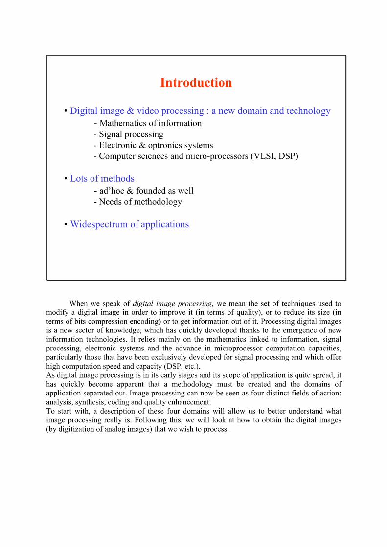
• Digital image & video processing : a new domain and technology
- Mathematics of information
- Signal processing
- Electronic & optronics systems
- Computer sciences and micro-processors (VLSI, DSP)
• Lots of methods
- ad’hoc & founded as well
- Needs of methodology
• Widespectrum of applications
When we speak of digital image processing, we mean the set of techniques used to
modify a digital image in order to improve it (in terms of quality), or to reduce its size (in
terms of bits compression encoding) or to get information out of it. Processing digital images
is a new sector of knowledge, which has quickly developed thanks to the emergence of new
information technologies. It relies mainly on the mathematics linked to information, signal
processing, electronic systems and the advance in microprocessor computation capacities,
particularly those that have been exclusively developed for signal processing and which offer
high computation speed and capacity (DSP, etc.).
As digital image processing is in its early stages and its scope of application is quite spread, it
has quickly become apparent that a methodology must be created and the domains of
application separated out. Image processing can now be seen as four distinct fields of action:
analysis, synthesis, coding and quality enhancement.
To start with, a description of these four domains will allow us to better understand what
image processing really is. Following this, we will look at how to obtain the digital images
(by digitization of analog images) that we wish to process.
2005 D. BARBA 3
Introduction
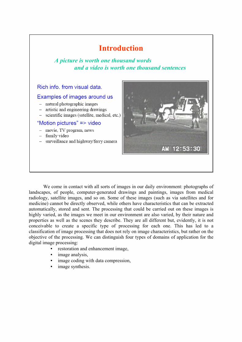
A picture is worth one thousand words
and a video is worth one thousand sentences
We come in contact with all sorts of images in our daily environment: photographs of
landscapes, of people, computer-generated drawings and paintings, images from medical
radiology, satellite images, and so on. Some of these images (such as via satellites and for
medicine) cannot be directly observed, while others have characteristics that can be extracted
automatically, stored and sent. The processing that could be carried out on these images is
highly varied, as the images we meet in our environment are also varied, by their nature and
properties as well as the scenes they describe. They are all different but, evidently, it is not
conceivable to create a specific type of processing for each one. This has led to a
classification of image processing that does not rely on image characteristics, but rather on the
objective of the processing. We can distinguish four types of domains of application for the
digital image processing:
• restoration and enhancement image,
• image analysis,
• image coding with data compression,
• image synthesis.
2005 D. BARBA 5
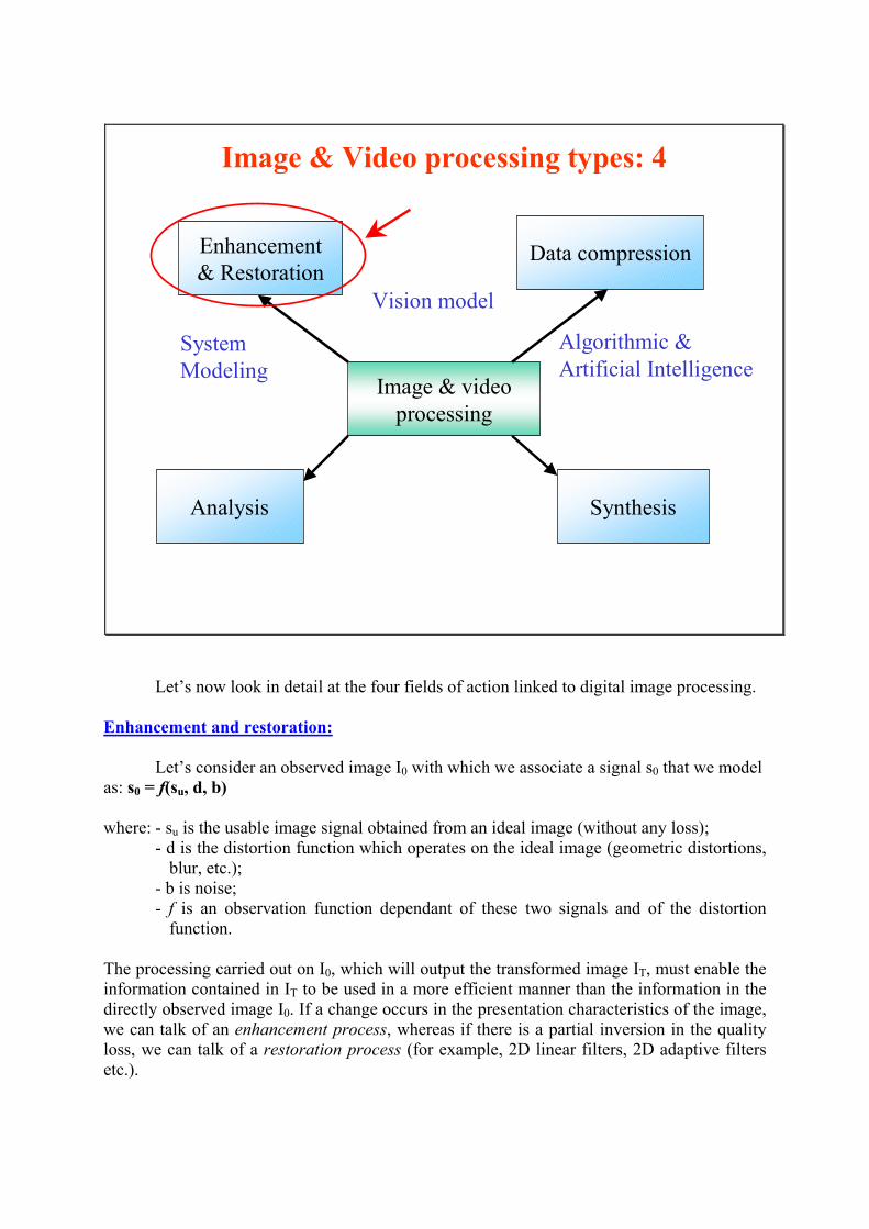
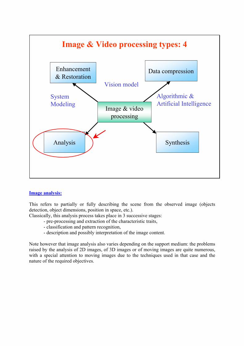
Image & Video processing types: 4
Analysis
Image & video
processing
Enhancement
& RestorationData compression
Synthesis
System
Modeling
Vision model
Algorithmic &
Artificial Intelligence
Let’s now look in detail at the four fields of action linked to digital image processing.
Enhancement and restoration:
Let’s consider an observed image I0 with which we associate a signal s0 that we model
as: s0 = f(su, d, b)
where: - su is the usable image signal obtained from an ideal image (without any loss);
- d is the distortion function which operates on the ideal image (geometric distortions,
blur, etc.);
- b is noise;
- f is an observation function dependant of these two signals and of the distortion
function.
The processing carried out on I0, which will output the transformed image IT, must enable the
information contained in IT to be used in a more efficient manner than the information in the
directly observed image I0. If a change occurs in the presentation characteristics of the image,
we can talk of an enhancement process, whereas if there is a partial inversion in the quality
loss, we can talk of a restoration process (for example, 2D linear filters, 2D adaptive filters
etc.).
2005 D. BARBA 5
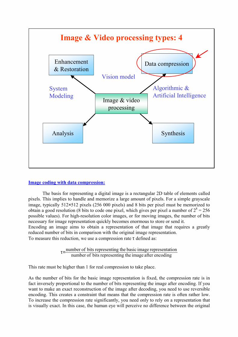
Image & Video processing types: 4
Analysis
Image & video
processing
Enhancement
& RestorationData compression
Synthesis
System
Modeling
Vision model
Algorithmic &
Artificial Intelligence
Image analysis:
This refers to partially or fully describing the scene from the observed image (objects
detection, object dimensions, position in space, etc.).
Classically, this analysis process takes place in 3 successive stages:
- pre-processing and extraction of the characteristic traits,
- classification and pattern recognition,
- description and possibly interpretation of the image content.
Note however that image analysis also varies depending on the support medium: the problems
raised by the analysis of 2D images, of 3D images or of moving images are quite numerous,
with a special attention to moving images due to the techniques used in that case and the
nature of the required objectives.
2005 D. BARBA 5
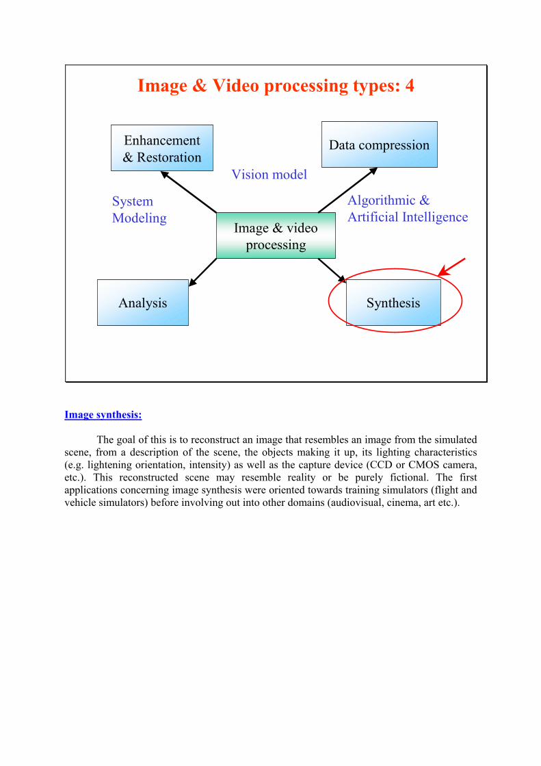
Image & Video processing types: 4
Analysis
Image & video
processing
Enhancement
& RestorationData compression
Synthesis
System
Modeling
Vision model
Algorithmic &
Artificial Intelligence
Image coding with data compression:
The basis for representing a digital image is a rectangular 2D table of elements called
pixels. This implies to handle and memorize a large amount of pixels. For a simple grayscale
image, typically 512×512 pixels (256 000 pixels) and 8 bits per pixel must be memorized to
obtain a good resolution (8 bits to code one pixel, which gives per pixel a number of 28 = 256
possible values). For high-resolution color images, or for moving images, the number of bits
necessary for image representation quickly becomes enormous to store or send it.
Encoding an image aims to obtain a representation of that image that requires a greatly
reduced number of bits in comparison with the original image representation.
To measure this reduction, we use a compression rate τ defined as:
encodingafter image thengrepresenti bits ofnumber
tionrepresenta image basic thengrepresenti bits ofnumber =τ
This rate must be higher than 1 for real compression to take place.
As the number of bits for the basic image representation is fixed, the compression rate is in
fact inversely proportional to the number of bits representing the image after encoding. If you
want to make an exact reconstruction of the image after decoding, you need to use reversible
encoding. This creates a constraint that means that the compression rate is often rather low.
To increase the compression rate significantly, you need only to rely on a representation that
is visually exact. In this case, the human eye will perceive no difference between the original

image and the image that is reconstituted after decoding. In addition, the complexity of the
encoding/decoding must be limited. Encoding a digital image involves finding a healthy
balance between the compression rate that will be high enough to make data storage and
transmission easier but that will not unduly affect the picture quality, and simultaneously
keeping in mind that decoding complexity must be restrained.
2005 D. BARBA 5
Image & Video processing types: 4
Analysis
Image & video
processing
Enhancement
& RestorationData compression
Synthesis
System
Modeling
Vision model
Algorithmic &
Artificial Intelligence
Image synthesis:
The goal of this is to reconstruct an image that resembles an image from the simulated
scene, from a description of the scene, the objects making it up, its lighting characteristics
(e.g. lightening orientation, intensity) as well as the capture device (CCD or CMOS camera,
etc.). This reconstructed scene may resemble reality or be purely fictional. The first
applications concerning image synthesis were oriented towards training simulators (flight and
vehicle simulators) before involving out into other domains (audiovisual, cinema, art etc.).

We should point out that image processing also relies on studies linked to the structure of
processing machines. An image contains a significant amount of data. In fact, for a moving
image there are N×M×P samples per second to process (N dots per line, M lines and P images
per second). Image processing requires powerful calculation capacity. It needs high
performance architectures with high degrees of parallelism and significant processing speeds.
Digital image processing has just been presented in accordance with the four main
domains of application. We can now look at this from another angle, by concentrating of the
nature of the processing results.
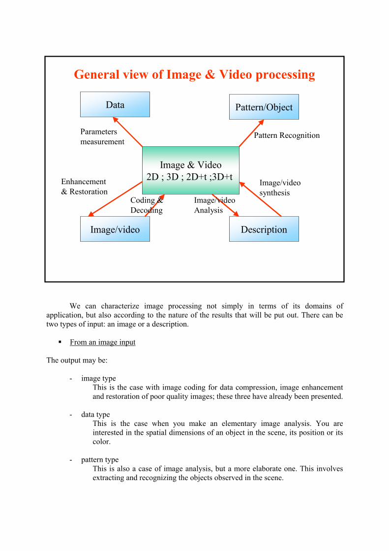
We can characterize image processing not simply in terms of its domains of
application, but also according to the nature of the results that will be put out. There can be
two types of input: an image or a description.
� From an image input
The output may be:
- image type
This is the case with image coding for data compression, image enhancement
and restoration of poor quality images; these three have already been presented.
- data type
This is the case when you make an elementary image analysis. You are
interested in the spatial dimensions of an object in the scene, its position or its
color.
- pattern type
This is also a case of image analysis, but a more elaborate one. This involves
extracting and recognizing the objects observed in the scene.
2005 D. BARBA 6
Image & Video
2D ; 3D ; 2D+t ;3D+t
Data
Image/video Description
Pattern/Object
Parameters
measurementPattern Recognition
Enhancement
& RestorationCoding &
Decoding
Image/video
Analysis
Image/video
synthesis
General view of Image & Video processing

- scene description type
This is also a possible output for an image analysis, but in the most advanced
version. The image is entirely broken up so that each object present in the
scene can be recognized. The scene is described in its totality and can be
interpreted.
� From a description input
For the output, the only expected type is an image. The domain of application involved is
image synthesis. We wish to reconstruct the image according to a given description. What
objects are present? What are their dimensions? Where are they in the scene? How are they
lit? What are the parameters (focal length, viewing angle etc.) of the camera doing the
filming?
You have now studied image processing from two different aspects: these aspects are
nevertheless strongly interconnected. We can now go on to look at the characteristics of the
signal that we wish to process: the image.
2005 D. BARBA 7
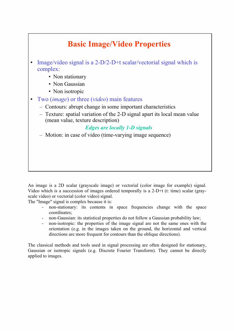
Basic Image/Video Properties
• Image/video signal is a 2-D/2-D+t scalar/vectorial signal which is complex:
• Non stationary
• Non Gaussian
• Non isotropic
• Two (image) or three (video) main features
– Contours: abrupt change in some important characteristics
– Texture: spatial variation of the 2-D signal apart its local mean value (mean value, texture description)
Edges are locally 1-D signals
– Motion: in case of video (time-varying image sequence)
An image is a 2D scalar (grayscale image) or vectorial (color image for example) signal.
Video which is a succession of images ordered temporally is a 2-D+t (t: time) scalar (gray-
scale video) or vectorial (color video) signal.
The "Image" signal is complex because it is:
- non-stationary: its contents in space frequencies change with the space
coordinates;
- non-Gaussian: its statistical properties do not follow a Gaussian probability law;
- non-isotropic: the properties of the image signal are not the same ones with the
orientation (e.g. in the images taken on the ground, the horizontal and vertical
directions are more frequent for contours than the oblique directions).
The classical methods and tools used in signal processing are often designed for stationary,
Gaussian or isotropic signals (e.g. Discrete Fourier Transform). They cannot be directly
applied to images.
Incidentally, images are mainly characterized by two types of element, namely contour and
texture:
- Contours are abrupt change of important characteristics from an area A to an area
B of a scene (average value, texture description). The edges can be locally
considered as 1D signals;
- Textures are spatial variation of the 2D signal apart its local mean value;
- Motion of the objects in a scene involves temporal modifications in the successive
frames of a video.
Now you have seen a general overview of images and digital image processing. In the
next part of this chapter, we will look at methods for representing images (digitizing and
encoding), which must be used in order to carry out digital processing. We will also see some
concrete examples of results relating to the domains of application that we explored earlier.
2005 D. BARBA 1
Examples of Image Processing
Images and Videos Analysis
Chapter 1
MULTIMEDIA SIGNAL PROCESSING
The four major domains of application for image processing have been globally
presented: what are the issues? what are the objectives? what methods to use? and which
tools? We will now look more closely at some concrete applications derived from these
different domains.
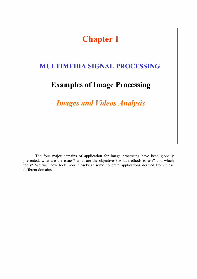
2005 D. BARBA 2
Image and video analysis
• Objectives
– Objects detection and extraction (segmentation)
Objects of interest
– Pattern recognition
Object classification, object identification
– Scene analysis and interpretation
• Relational
• Quantitative description
• Qualitative description
The first domain that interests us is image analysis. This covers a large number of
potential applications and is probably the domain for which there is the greatest variety of
examples (medical analysis, classification of chromosomes, automatic reading, signature
verification, remote sensing, segmentation and classification of geographical areas, etc.).
We can however suggest a typical image analysis cycle, which consists of
� Detecting the different objects present in a scene and extracting them
(segmentation, slicing into areas).
� Characterizing the objects in the picture (size, location, etc.).
� Recognizing objects and classifying them.
� Analyzing and interpreting the scene according to the previous results. The
scene could for example be described quantitatively and/or qualitatively.
Let us remember though that the applications are quite varied and that the global approach
given here may sometimes require changes in the stages of processing, according to the
difficulties encountered.
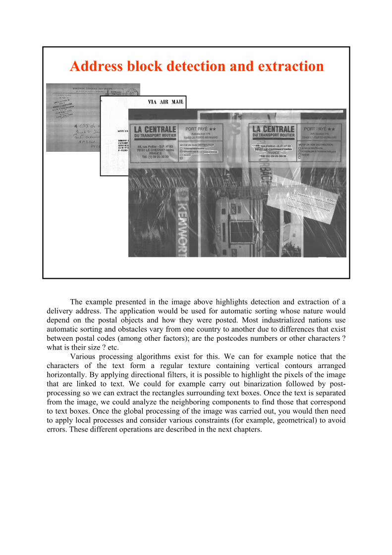
The example presented in the image above highlights detection and extraction of a
delivery address. The application would be used for automatic sorting whose nature would
depend on the postal objects and how they were posted. Most industrialized nations use
automatic sorting and obstacles vary from one country to another due to differences that exist
between postal codes (among other factors); are the postcodes numbers or other characters ?
what is their size ? etc.
Various processing algorithms exist for this. We can for example notice that the
characters of the text form a regular texture containing vertical contours arranged
horizontally. By applying directional filters, it is possible to highlight the pixels of the image
that are linked to text. We could for example carry out binarization followed by post-
processing so we can extract the rectangles surrounding text boxes. Once the text is separated
from the image, we could analyze the neighboring components to find those that correspond
to text boxes. Once the global processing of the image was carried out, you would then need
to apply local processes and consider various constraints (for example, geometrical) to avoid
errors. These different operations are described in the next chapters.
2005 D. BARBA 3
Address block detection and extraction
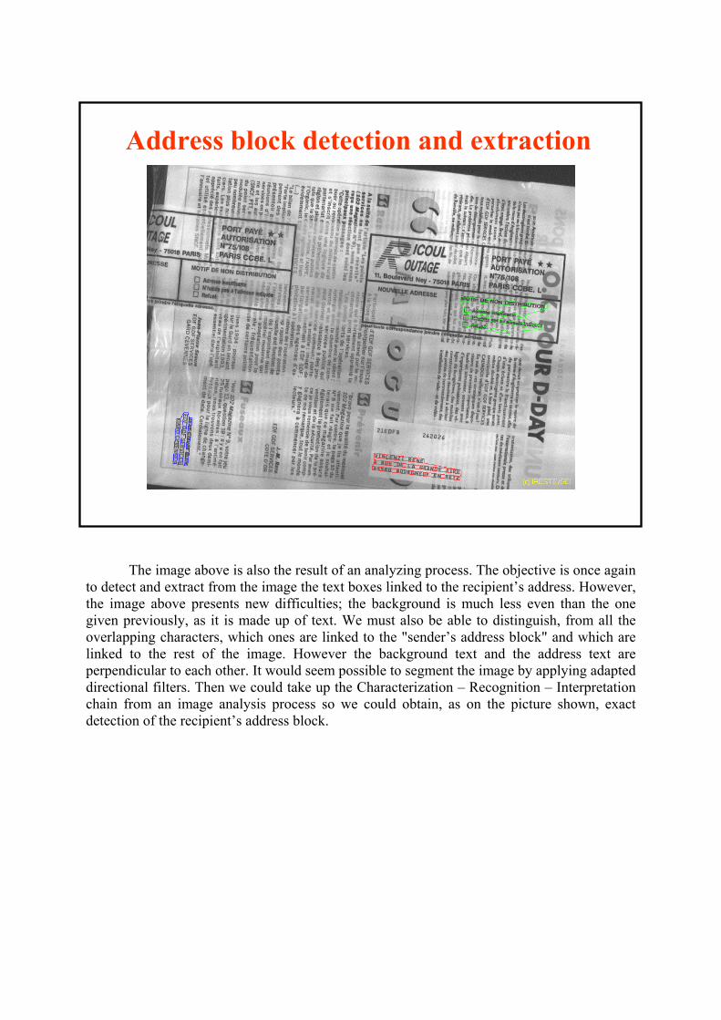
The image above is also the result of an analyzing process. The objective is once again
to detect and extract from the image the text boxes linked to the recipient’s address. However,
the image above presents new difficulties; the background is much less even than the one
given previously, as it is made up of text. We must also be able to distinguish, from all the
overlapping characters, which ones are linked to the "sender’s address block" and which are
linked to the rest of the image. However the background text and the address text are
perpendicular to each other. It would seem possible to segment the image by applying adapted
directional filters. Then we could take up the Characterization – Recognition – Interpretation
chain from an image analysis process so we could obtain, as on the picture shown, exact
detection of the recipient’s address block.
2005 D. BARBA 1
Address block detection and extraction
2005 D. BARBA 5
Extracting and reading the amount
written on a cheque
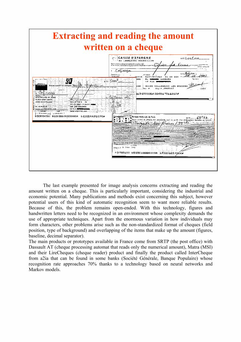
The last example presented for image analysis concerns extracting and reading the
amount written on a cheque. This is particularly important, considering the industrial and
economic potential. Many publications and methods exist concerning this subject, however
potential users of this kind of automatic recognition seem to want more reliable results.
Because of this, the problem remains open-ended. With this technology, figures and
handwritten letters need to be recognized in an environment whose complexity demands the
use of appropriate techniques. Apart from the enormous variation in how individuals may
form characters, other problems arise such as the non-standardized format of cheques (field
position, type of background) and overlapping of the items that make up the amount (figures,
baseline, decimal separator).
The main products or prototypes available in France come from SRTP (the post office) with
Dassault AT (cheque processing automat that reads only the numerical amount), Matra (MSI)
and their LireCheques (cheque reader) product and finally the product called InterCheque
from a2ia that can be found in some banks (Société Générale, Banque Populaire) whose
recognition rate approaches 70% thanks to a technology based on neural networks and
Markov models.
2005 D. BARBA 6
Image and Video Coding
with Data Compression
Examples of Image Processing
After these few examples of image analysis applications, we are going to look now at
applications linked to image encoding for data compression.
2005 D. BARBA 7
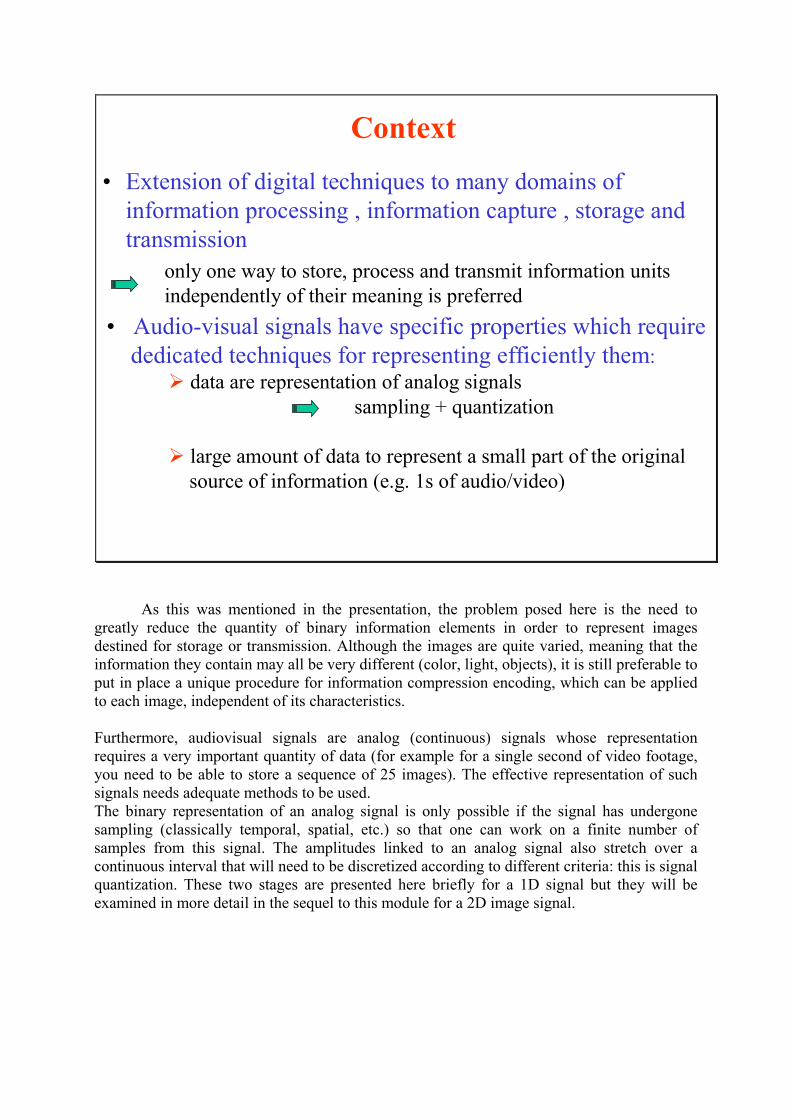
Context
• Extension of digital techniques to many domains of
information processing , information capture , storage and
transmission
only one way to store, process and transmit information units
independently of their meaning is preferred
• Audio-visual signals have specific properties which require
dedicated techniques for representing efficiently them:
� data are representation of analog signals
sampling + quantization
� large amount of data to represent a small part of the original
source of information (e.g. 1s of audio/video)
As this was mentioned in the presentation, the problem posed here is the need to
greatly reduce the quantity of binary information elements in order to represent images
destined for storage or transmission. Although the images are quite varied, meaning that the
information they contain may all be very different (color, light, objects), it is still preferable to
put in place a unique procedure for information compression encoding, which can be applied
to each image, independent of its characteristics.
Furthermore, audiovisual signals are analog (continuous) signals whose representation
requires a very important quantity of data (for example for a single second of video footage,
you need to be able to store a sequence of 25 images). The effective representation of such
signals needs adequate methods to be used.
The binary representation of an analog signal is only possible if the signal has undergone
sampling (classically temporal, spatial, etc.) so that one can work on a finite number of
samples from this signal. The amplitudes linked to an analog signal also stretch over a
continuous interval that will need to be discretized according to different criteria: this is signal
quantization. These two stages are presented here briefly for a 1D signal but they will be
examined in more detail in the sequel to this module for a 2D image signal.
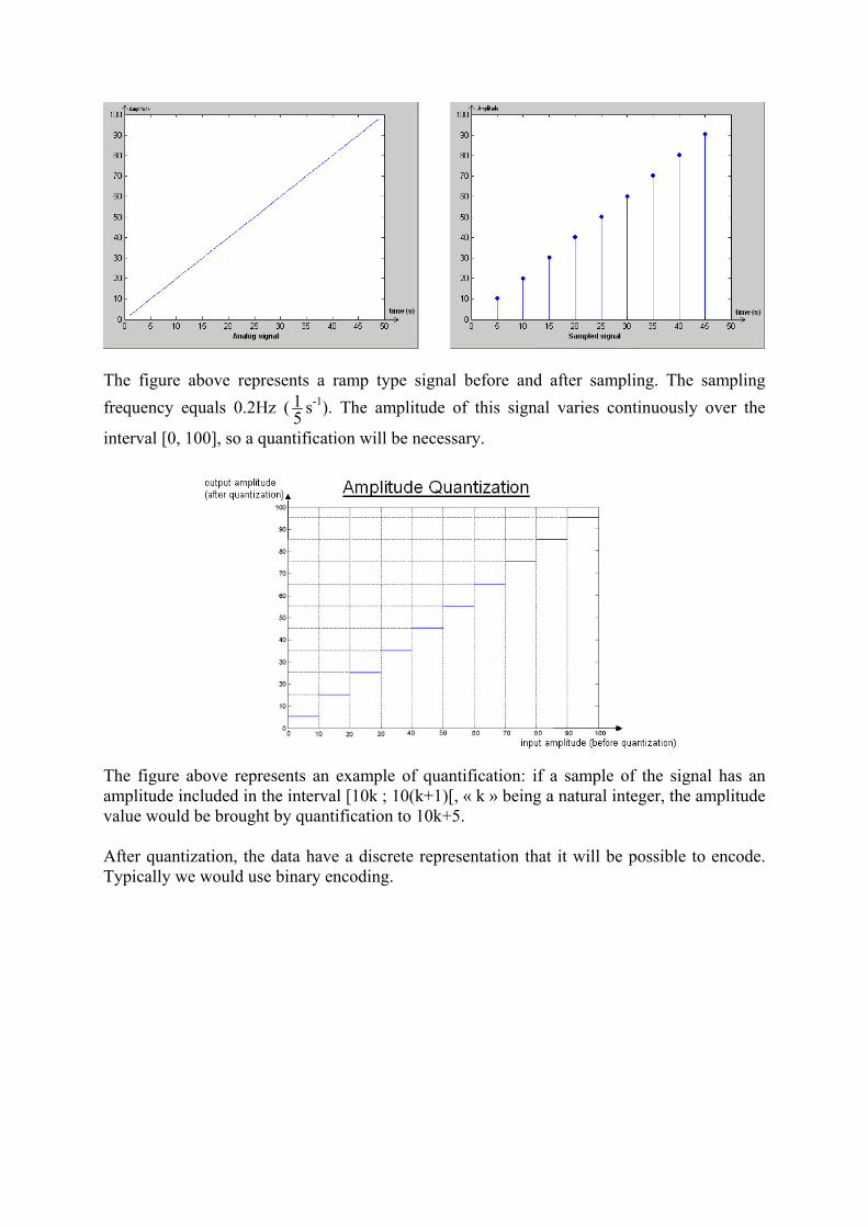
The figure above represents a ramp type signal before and after sampling. The sampling
frequency equals 0.2Hz (51 s
-1). The amplitude of this signal varies continuously over the
interval [0, 100], so a quantification will be necessary.
The figure above represents an example of quantification: if a sample of the signal has an
amplitude included in the interval [10k ; 10(k+1)[, « k » being a natural integer, the amplitude
value would be brought by quantification to 10k+5.
After quantization, the data have a discrete representation that it will be possible to encode.
Typically we would use binary encoding.
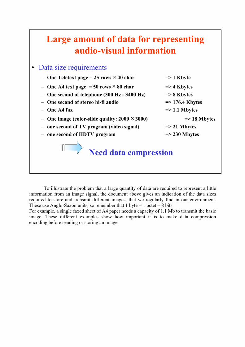
2005 D. BARBA 9
• Data size requirements
– One Teletext page = 25 rows × 40 char => 1 Kbyte
– One A4 text page = 50 rows × 80 char => 4 Kbytes
– One second of telephone (300 Hz - 3400 Hz) => 8 Kbytes
– One second of stereo hi-fi audio => 176.4 Kbytes
– One A4 fax => 1.1 Mbytes
– One image (color-slide quality: 2000 × 3000) => 18 Mbytes
– one second of TV program (video signal) => 21 Mbytes
– one second of HDTV program => 230 Mbytes
Need data compression
Large amount of data for representing
audio-visual information
To illustrate the problem that a large quantity of data are required to represent a little
information from an image signal, the document above gives an indication of the data sizes
required to store and transmit different images, that we regularly find in our environment.
These use Anglo-Saxon units, so remember that 1 byte = 1 octet = 8 bits.
For example, a single faxed sheet of A4 paper needs a capacity of 1.1 Mb to transmit the basic
image. These different examples show how important it is to make data compression
encoding before sending or storing an image.
2005 D. BARBA 10
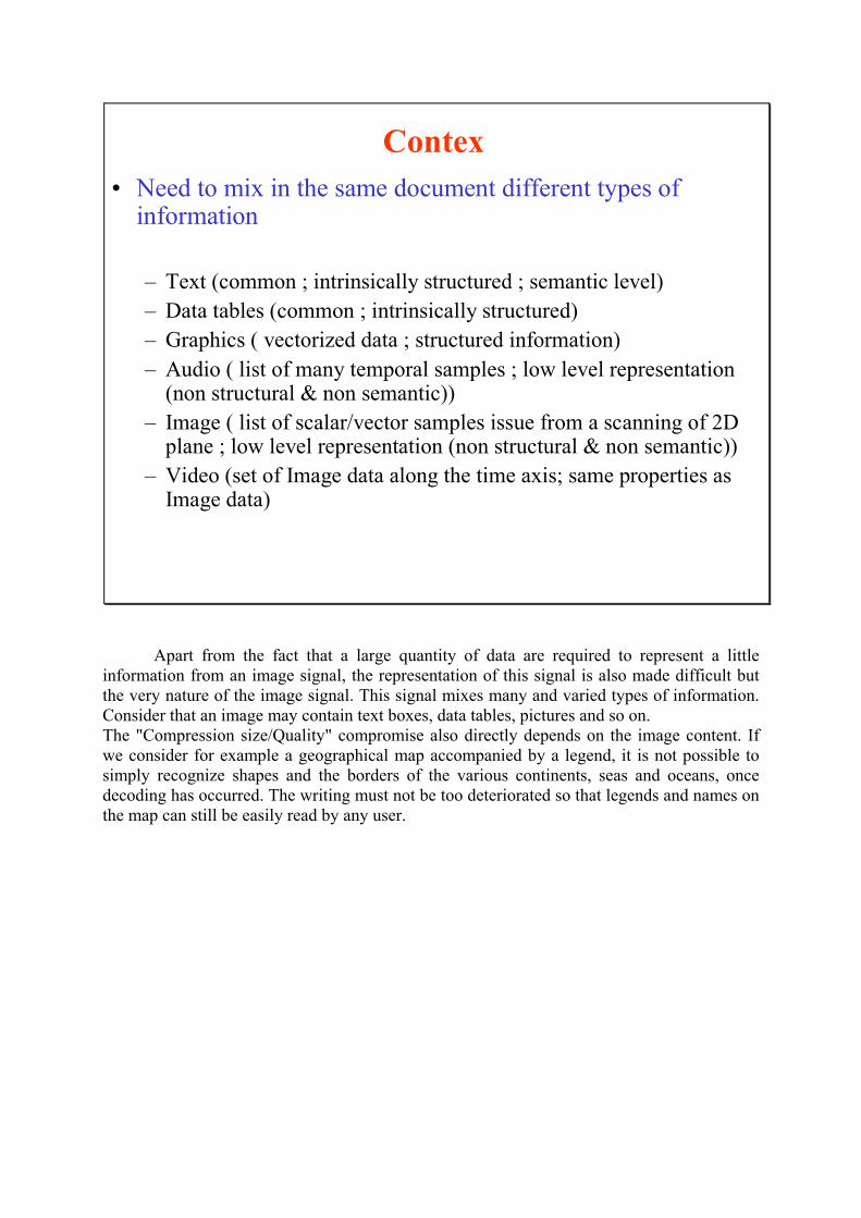
Contex
• Need to mix in the same document different types of information
– Text (common ; intrinsically structured ; semantic level)
– Data tables (common ; intrinsically structured)
– Graphics ( vectorized data ; structured information)
– Audio ( list of many temporal samples ; low level representation(non structural & non semantic))
– Image ( list of scalar/vector samples issue from a scanning of 2D plane ; low level representation (non structural & non semantic))
– Video (set of Image data along the time axis; same properties asImage data)
Apart from the fact that a large quantity of data are required to represent a little
information from an image signal, the representation of this signal is also made difficult but
the very nature of the image signal. This signal mixes many and varied types of information.
Consider that an image may contain text boxes, data tables, pictures and so on.
The "Compression size/Quality" compromise also directly depends on the image content. If
we consider for example a geographical map accompanied by a legend, it is not possible to
simply recognize shapes and the borders of the various continents, seas and oceans, once
decoding has occurred. The writing must not be too deteriorated so that legends and names on
the map can still be easily read by any user.
2005 D. BARBA 8
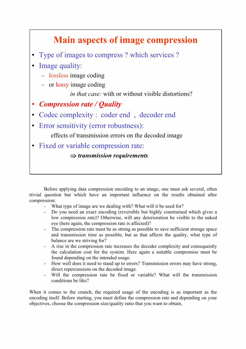
Main aspects of image compression
• Type of images to compress ? which services ?
• Image quality:
– lossless image coding
– or lossy image coding
in that case: with or without visible distortions?
• Compression rate / Quality
• Codec complexity : coder end , decoder end
• Error sensitivity (error robustness):
effects of transmission errors on the decoded image
• Fixed or variable compression rate:
⇒⇒⇒⇒ transmission requirements
Before applying data compression encoding to an image, one must ask several, often
trivial question but which have an important influence on the results obtained after
compression:
- What type of image are we dealing with? What will it be used for?
- Do you need an exact encoding (reversible but highly constrained which gives a
low compression rate)? Otherwise, will any deterioration be visible to the naked
eye (here again, the compression rate is affected)?
- The compression rate must be as strong as possible to save sufficient storage space
and transmission time as possible, but as that affects the quality, what type of
balance are we striving for?
- A rise in the compression rate increases the decoder complexity and consequently
the calculation cost for the system. Here again a suitable compromise must be
found depending on the intended usage.
- How well does it need to stand up to errors? Transmission errors may have strong,
direct repercussions on the decoded image.
- Will the compression rate be fixed or variable? What will the transmission
conditions be like?
When it comes to the crunch, the required usage of the encoding is as important as the
encoding itself. Before starting, you must define the compression rate and depending on your
objectives, choose the compression size/quality ratio that you want to obtain.
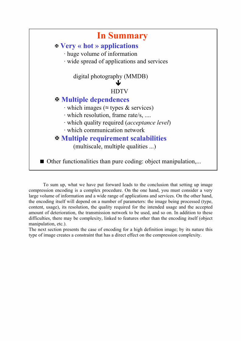
2005 D. BARBA 11
�Very « hot » applications· huge volume of information
· wide spread of applications and services
digital photography (MMDB)
�
HDTV
�Multiple dependences· which images (≈ types & services)
· which resolution, frame rate/s, ....
· which quality required (acceptance level)
· which communication network
�Multiple requirement scalabilities(multiscale, multiple qualities ...)
� Other functionalities than pure coding: object manipulation,...
In Summary
To sum up, what we have put forward leads to the conclusion that setting up image
compression encoding is a complex procedure. On the one hand, you must consider a very
large volume of information and a wide range of applications and services. On the other hand,
the encoding itself will depend on a number of parameters: the image being processed (type,
content, usage), its resolution, the quality required for the intended usage and the accepted
amount of deterioration, the transmission network to be used, and so on. In addition to these
difficulties, there may be complexity, linked to features other than the encoding itself (object
manipulation, etc.).
The next section presents the case of encoding for a high definition image; by its nature this
type of image creates a constraint that has a direct effect on the compression complexity.
2005 D. BARBA 12
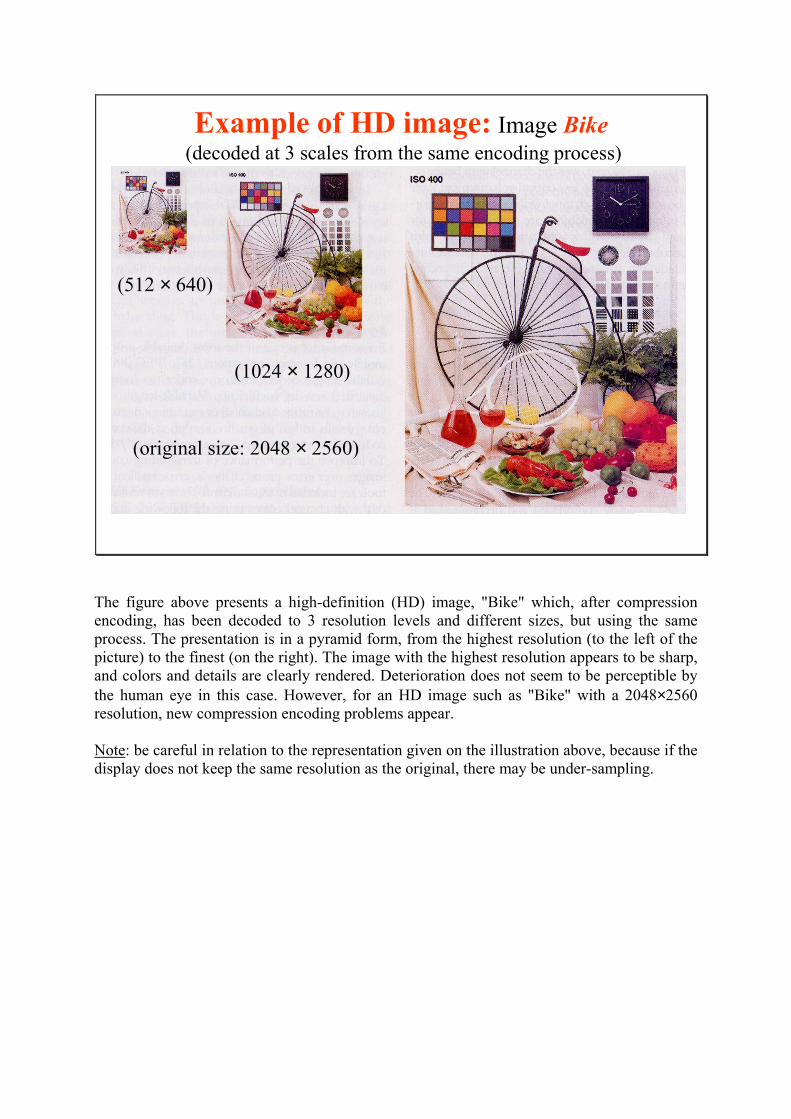
Example of HD image: Image Bike(decoded at 3 scales from the same encoding process)
(1024 × 1280)
(512 × 640)
(original size: 2048 × 2560)
The figure above presents a high-definition (HD) image, "Bike" which, after compression
encoding, has been decoded to 3 resolution levels and different sizes, but using the same
process. The presentation is in a pyramid form, from the highest resolution (to the left of the
picture) to the finest (on the right). The image with the highest resolution appears to be sharp,
and colors and details are clearly rendered. Deterioration does not seem to be perceptible by
the human eye in this case. However, for an HD image such as "Bike" with a 2048×2560 resolution, new compression encoding problems appear.
Note: be careful in relation to the representation given on the illustration above, because if the
display does not keep the same resolution as the original, there may be under-sampling.
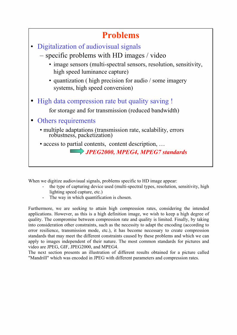
2005 D. BARBA 13
• High data compression rate but quality saving !
for storage and for transmission (reduced bandwidth)
• Others requirements
• multiple adaptations (transmission rate, scalability, errors robustness, packetization)
• access to partial contents, content description, …
JPEG2000, MPEG4, MPEG7 standards
Problems
• Digitalization of audiovisual signals
– specific problems with HD images / video
• image sensors (multi-spectral sensors, resolution, sensitivity,
high speed luminance capture)
• quantization ( high precision for audio / some imagery
systems, high speed conversion)
When we digitize audiovisual signals, problems specific to HD image appear:
- the type of capturing device used (multi-spectral types, resolution, sensitivity, high
lighting speed capture, etc.)
- The way in which quantification is chosen.
Furthermore, we are seeking to attain high compression rates, considering the intended
applications. However, as this is a high definition image, we wish to keep a high degree of
quality. The compromise between compression rate and quality is limited. Finally, by taking
into consideration other constraints, such as the necessity to adapt the encoding (according to
error resilience, transmission mode, etc.), it has become necessary to create compression
standards that may meet the different constraints caused by these problems and which we can
apply to images independent of their nature. The most common standards for pictures and
video are JPEG, GIF, JPEG2000, and MPEG4.
The next section presents an illustration of different results obtained for a picture called
"Mandrill" which was encoded in JPEG with different parameters and compression rates.
2005 D. BARBA 14
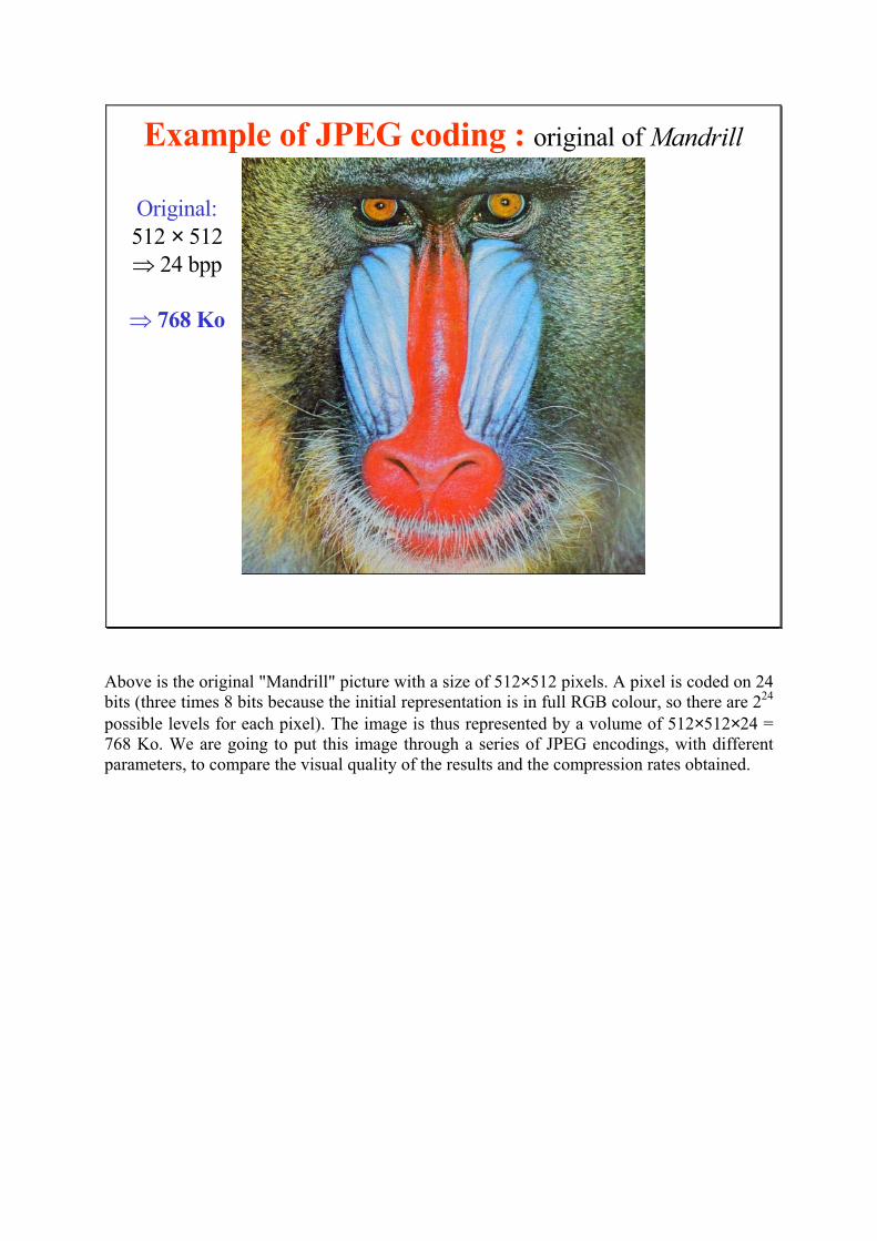
Example of JPEG coding : original of Mandrill
Original:
512 × 512
⇒ 24 bpp
⇒ 768 Ko
Above is the original "Mandrill" picture with a size of 512×512 pixels. A pixel is coded on 24 bits (three times 8 bits because the initial representation is in full RGB colour, so there are 2
24
possible levels for each pixel). The image is thus represented by a volume of 512×512×24 = 768 Ko. We are going to put this image through a series of JPEG encodings, with different
parameters, to compare the visual quality of the results and the compression rates obtained.
2005 D. BARBA 15
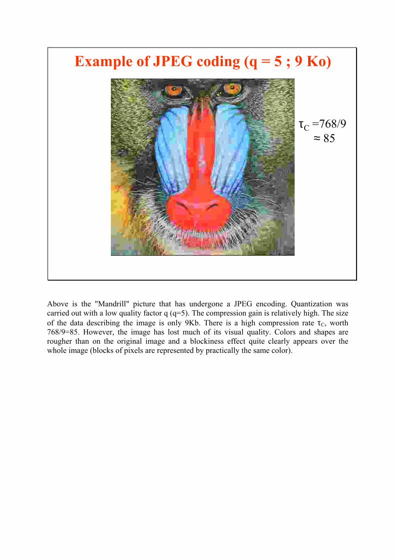
Example of JPEG coding (q = 5 ; 9 Ko)
τC =768/9≈ 85
Above is the "Mandrill" picture that has undergone a JPEG encoding. Quantization was
carried out with a low quality factor q (q=5). The compression gain is relatively high. The size
of the data describing the image is only 9Kb. There is a high compression rate τC, worth 768/9=85. However, the image has lost much of its visual quality. Colors and shapes are
rougher than on the original image and a blockiness effect quite clearly appears over the
whole image (blocks of pixels are represented by practically the same color).
2005 D. BARBA 16
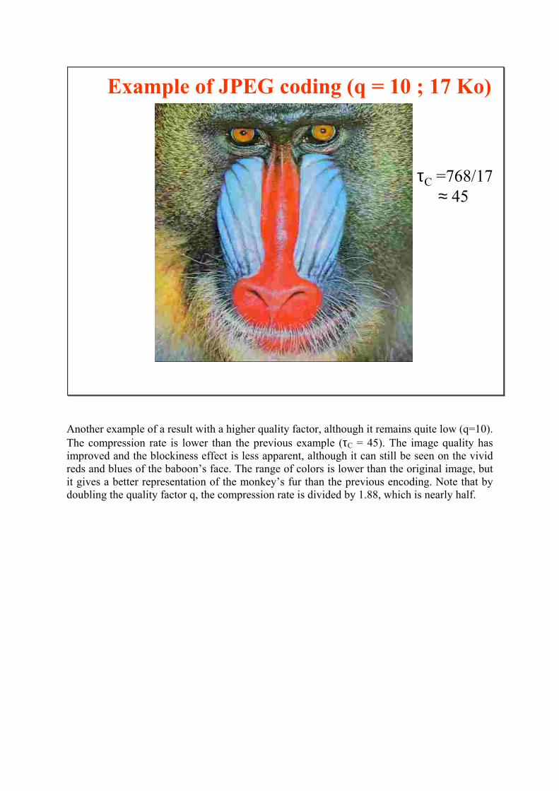
Example of JPEG coding (q = 10 ; 17 Ko)
τC =768/17≈ 45
Another example of a result with a higher quality factor, although it remains quite low (q=10).
The compression rate is lower than the previous example (τC = 45). The image quality has
improved and the blockiness effect is less apparent, although it can still be seen on the vivid
reds and blues of the baboon’s face. The range of colors is lower than the original image, but
it gives a better representation of the monkey’s fur than the previous encoding. Note that by
doubling the quality factor q, the compression rate is divided by 1.88, which is nearly half.
2005 D. BARBA 17
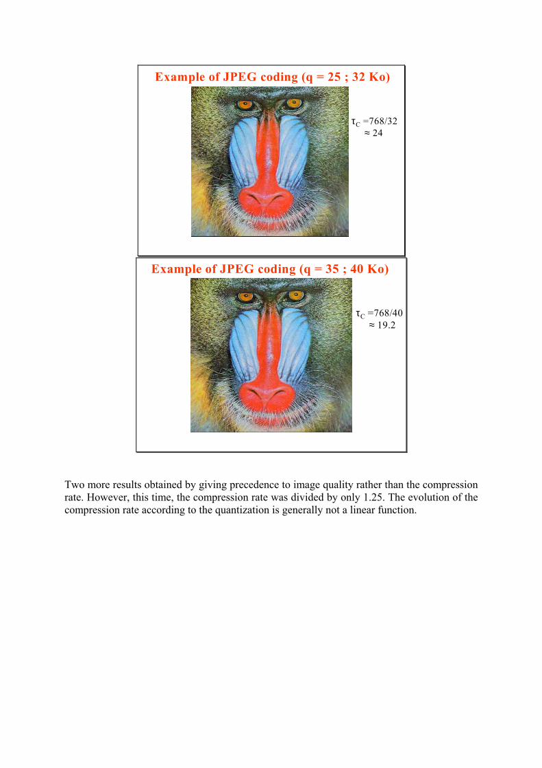
Example of JPEG coding (q = 25 ; 32 Ko)
τC =768/32
≈ 24
2005 D. BARBA 18
Example of JPEG coding (q = 35 ; 40 Ko)
τC =768/40
≈ 19.2
Two more results obtained by giving precedence to image quality rather than the compression
rate. However, this time, the compression rate was divided by only 1.25. The evolution of the
compression rate according to the quantization is generally not a linear function.
2005 D. BARBA 20
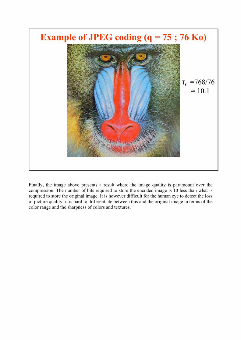
Example of JPEG coding (q = 75 ; 76 Ko)
τC =768/76≈ 10.1
Finally, the image above presents a result where the image quality is paramount over the
compression. The number of bits required to store the encoded image is 10 less than what is
required to store the original image. It is however difficult for the human eye to detect the loss
of picture quality: it is hard to differentiate between this and the original image in terms of the
color range and the sharpness of colors and textures.

Here we have presented image processing under its different aspects. It was created
from new requirements made by information technology, and in turn uses those same
technologies to ensure its rapid development. With its expansion, four wide domains of
application have appeared: restoration, encoding, analysis and image synthesis.
In this course, the domains of analysis and encoding have been accompanied by examples of
concrete applications, in order to give an initial view of the possibilities and results offered by
the various image processing.
However, in the real world, the images that surround us cannot generally be processed
directly and they are not digital. They need to be digitized in order to be processed with
adapted algorithms and systems. This digitizing stage will be looked at in the next resource
(Image digitization).
Exercise Chapter 1– Introduction to Matlab
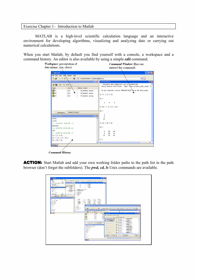
MATLAB is a high-level scientific calculation language and an interactive
environment for developing algorithms, visualizing and analyzing date or carrying out
numerical calculations.
When you start Matlab, by default you find yourself with a console, a workspace and a
command history. An editor is also available by using a simple edit command.
ACTIONACTIONACTIONACTION: Start Matlab and add your own working folder paths to the path list in the path
browser (don’t forget the subfolders). The pwd, cd, ls Unix commands are available.
Note: when a user runs a command in the console, Matlab will go looking in the folder that
you indicated in the path browser; if a function or a script matches that command, the first
one found will be the one used (so take care with the folder order and the names of scripts
and functions).
Exercise 1 – Operators
Between each exercise, we recommend that you use the clear and close all commands so that
you can empty the workspace and close all the figures.
1.1 – Enter the command a=[1 4 5 ;4 8 9], what does this command correspond to?
In the console, enter the a=rand(5) command. Then enter the help rand command to get a
description of the operation carried out by the rand function. Finally, enter the command:
a=rand(5) followed by a semi-colon « ; »
What difference can we observe in the console with the a=rand(5) command? Deduce from t
his the role of the « ; »in Matlab.
1.2 – In Matlab, the « : » operator is very useful. It can be used, among other things, to swap
elements from a row or a column of a matrix.
A word of caution: the index 0 does not exist in Matlab. the first element of a matrix is
accessed by an index of 1. For example array(1,1) for images accesses the value of the pixel
(1st row, 1
st column). The first index is for the rows, the second index for the columns.
To fully understand these concepts, try the commands:
- a(2,1)
- a(1:3,1)
- a( :,2)
- a(1, :)
- a([1 4], :)
- a(1 :2 :5, :) (the 1:2:5 command sweeps the interval [1,5] by steps of 2)
Be careful however not to put a « ; » at the end of a row to visualize the results obtained in the
console.
1.3 – Matlab is an interesting tool for matrix calculations. The various classical matrix
operations (addition, multiplication, eigenvalues etc.) are there of course but there are also
element by element operations that are very useful in image processing; these are available
through a specific operator (for example: « .* », « ./ »). Enter the following commands (without « ; » at the end of the line to see the results):
- a= [0 0 0; 1 1 1; 2 2 2]
- b=a+4
- c=a*b
- e=a.*b
Explain the difference between « c » and « e ».
ACTION:ACTION:ACTION:ACTION: Create a matrix A sized 4×4 using the method of your choice (use rand or enter
the items one by one). How can you access:
- the first row of A?
- the fourth column of A?
- the first three items of the fourth row in A?
Exercise 2 – Display
Matlab also offers a wide range of diverse and practical display possibilities. For example,
you can plot function on a logarithmic scale or view the values of a matrix as an image.
2.1 – A vector can be displayed using the plot command. Enter the help plot command to
obtain more information about this function and on functions with similar properties
(subplot, semilogx, etc.).
Try out the following commands:
- x=1:3:10
- plot(x) then plot(x,’r’)
- y=rand(4,1), then plot(y), then plot(x,y,’g’). Interpret the difference between these
two commands.
The plot function is very useful for obtaining for example the curves of different plane
functions.
2.2 – Displaying a matrix on the other hand corresponds to displaying an image. Each item (n,
m) in the matrix is considered as having the value of the pixel (n, m) with which it is
associated. Check this by entering the following commands:
- a=rand(10)*10 ; (so that the elements are not limited to [0,1])
- a=exp(a) ; (to obtain larger spans between the items of vector a)
- image(a)
Images can be displayed with the image, imagesc, and imshow functions. Try zooming with
the mouse; what kind of interpolation is used?
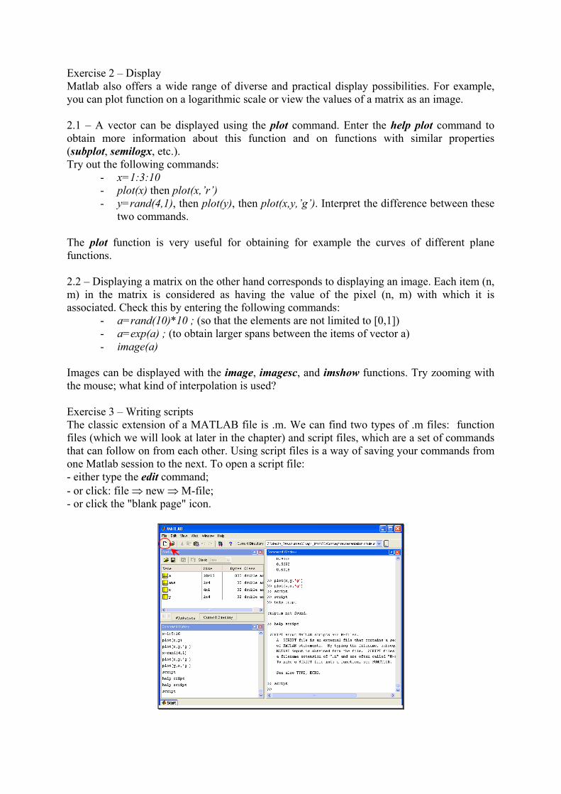
Exercise 3 – Writing scripts
The classic extension of a MATLAB file is .m. We can find two types of .m files: function
files (which we will look at later in the chapter) and script files, which are a set of commands
that can follow on from each other. Using script files is a way of saving your commands from
one Matlab session to the next. To open a script file:
- either type the edit command;
- or click: file ⇒ new ⇒ M-file; - or click the "blank page" icon.
To run a script:
- either run a file_name command in the command window (without the .m
extension), making sure that the path list is consistent.
- or select lines from the .m file in the edit window and press the F9 key (a practical
way of running only part of a script).
ACTIONACTIONACTIONACTION: Enter all the commands from the section 1.2 into a script and save it (for
example: test.m). Run the script in the console and using the F9 key.
Exercise 4 – Data types
During this series of exercises, we are going to be using the Image Processing toolbox. This
contains a large number of existing functions (do not hesitate to look in the help using the
help or helpwin commands), as well as demonstrations. Sometimes we will use our own
functions and sometimes we will be using those from the toolbox. However, you need to be
careful with the data types. Classically and by default in Matlab, everything is a matrix of
double, but most of the functions in the Image Processing toolbox work with the uint8 type to
represent pixel value. You will need to convert the type each time this proves necessary (you
can easily see the type of your data in the workspace).
ACTIONACTIONACTIONACTION: From the image base, download the ‘FRUIT_LUMI’ image into your working
folder. Read and display the image file respectively using the commands imread and imshow:
fruit = imread(‘FRUIT_LUMI.bmp’);
imshow(fruit);
By consulting the workspace, look at the size and data type. So as to display a sub-image that
corresponds to the top left corner of 64×64 pixels, test this command: imshow(fruit(1:64,1:64));
The matrix fruit now represents the ‘FRUIT_LUMI’ image. Try adding this matrix directly to
any number (e.g.: fruit+8). The console returns an error message:
Function ’+’ is not defined for values of class ’uint8’
This is because the ‘+’ operator is defined only for "double" type elements. To carry out this
operation, you will need to force the "double" type for the elements in the matrix by typing:
double(fruit). Try again after this conversion.
Exercise 5 – Writing your functions
Use the function files as you would in any classical imperative programming situation. These
are also .m files. To use a function, you must call it with call parameters either in a script or in
another function.
ACTIONACTIONACTIONACTION: Use the template.m file to write your own max_min function that will find the
difference between the largest and smallest element in a matrix. You can use the Matlab max
and min functions. Be careful to save the name of your function (e.g. max_min) in a file of
the same name (example max_min.m).
Contents of the template.m file:
function[out1, out2] = template(arg1, arg2)
%--------------------------------------------
%
% Description:
%
% Input:
% arg1:
% arg2:
%
% Output:
% out1:
% out2:
%
% Date:
% Modif:
%---------------------------------------------
Note: You can use a function directly in the command window (providing that you use the
correct paths) or within a script or another function.
Solution to the exercise for the introduction to Matlab
The first objective of this exercise is to make yo u familiar with Matlab if you have never used it before and to remi nd current users of its basic functions. 1 – Operators 1.2 –
The command a=[1 4 5 ;4 8 9] returns the matrix 2 ×3:
981541
.
The command a=rand(5) returns a matrix 5 ×5 made up of random values between 0 and 1. Finally, in Matlab, the operator « ; » is used when you do not want to display a command’s result in the console. This op erator is useful, for example when you work with large matrices (such as images), which are sometimes long to display and often not very repres entative of the data. 1.3 – Working with the operator « : ». 1.4 – In Matlab There are two types of matrix operations that use the « * » and « / » operators:
- matrix multiplication and division, - element by element multiplication and division (joi nt use with the
operator « . ». The command c=a*b will perform a matrix multiplication of matrix « a » by
matrix « b » : ∑=k
kjikij bac . .
The command e=a.*b will perform an element by element multiplication of
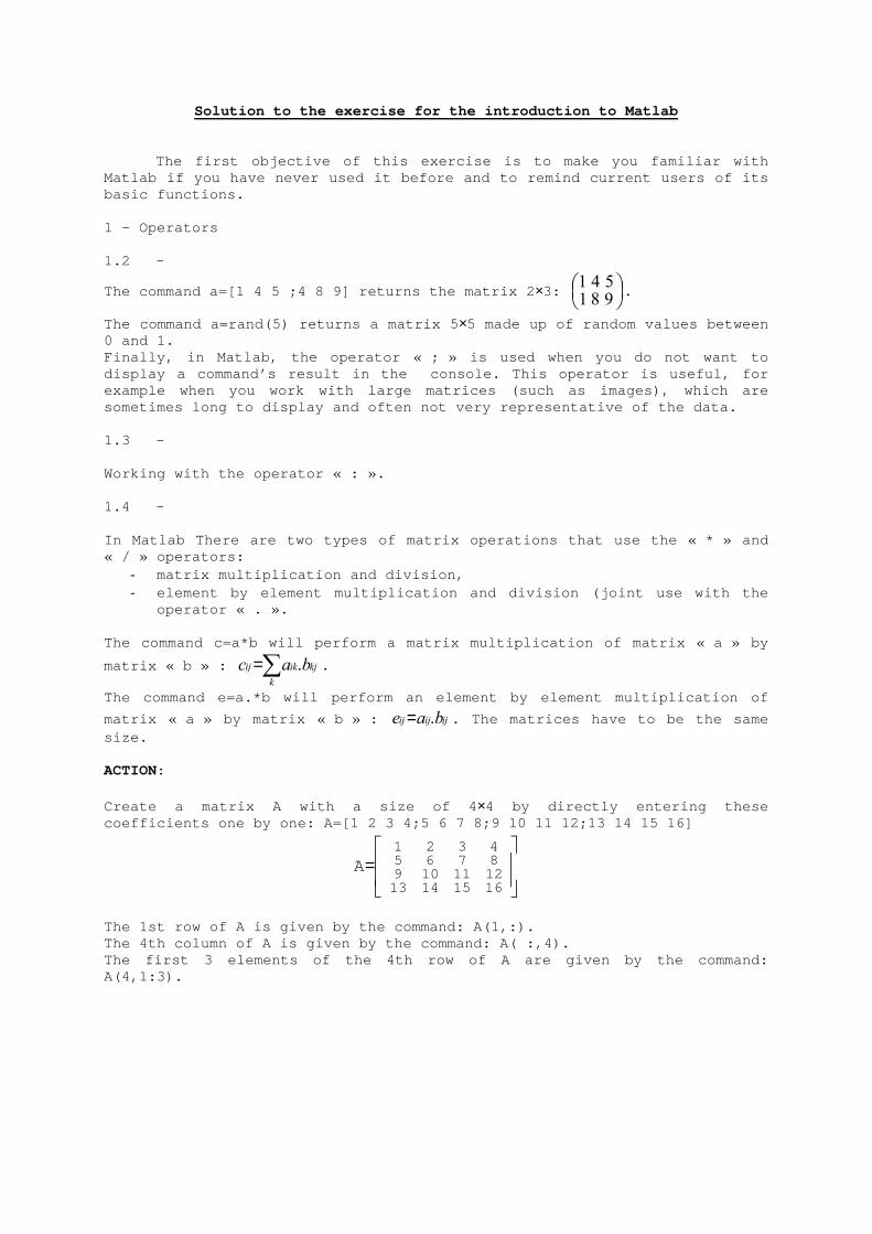
matrix « a » by matrix « b » : ijijij bae .= . The matrices have to be the same size. ACTION: Create a matrix A with a size of 4 ×4 by directly entering these coefficients one by one: A=[1 2 3 4;5 6 7 8;9 10 11 12;13 14 15 16]
=
16 151413121110987654321
A
The 1st row of A is given by the command: A(1,:). The 4th column of A is given by the command: A( :,4). The first 3 elements of the 4th row of A are given by the command: A(4,1:3).
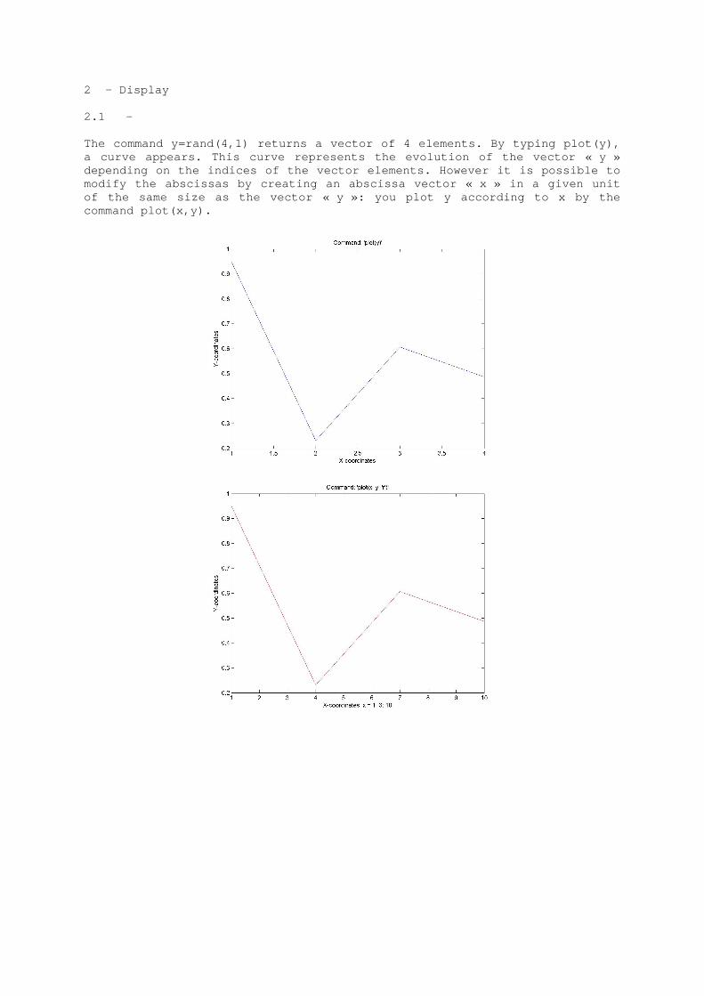
2 – Display 2.1 – The command y=rand(4,1) returns a vector of 4 elements. By typing plot(y), a curve appears. This curve represents the evolutio n of the vector « y » depending on the indices of the vector elements. Ho wever it is possible to modify the abscissas by creating an abscissa vector « x » in a given unit of the same size as the vector « y »: you plot y ac cording to x by the command plot(x,y).
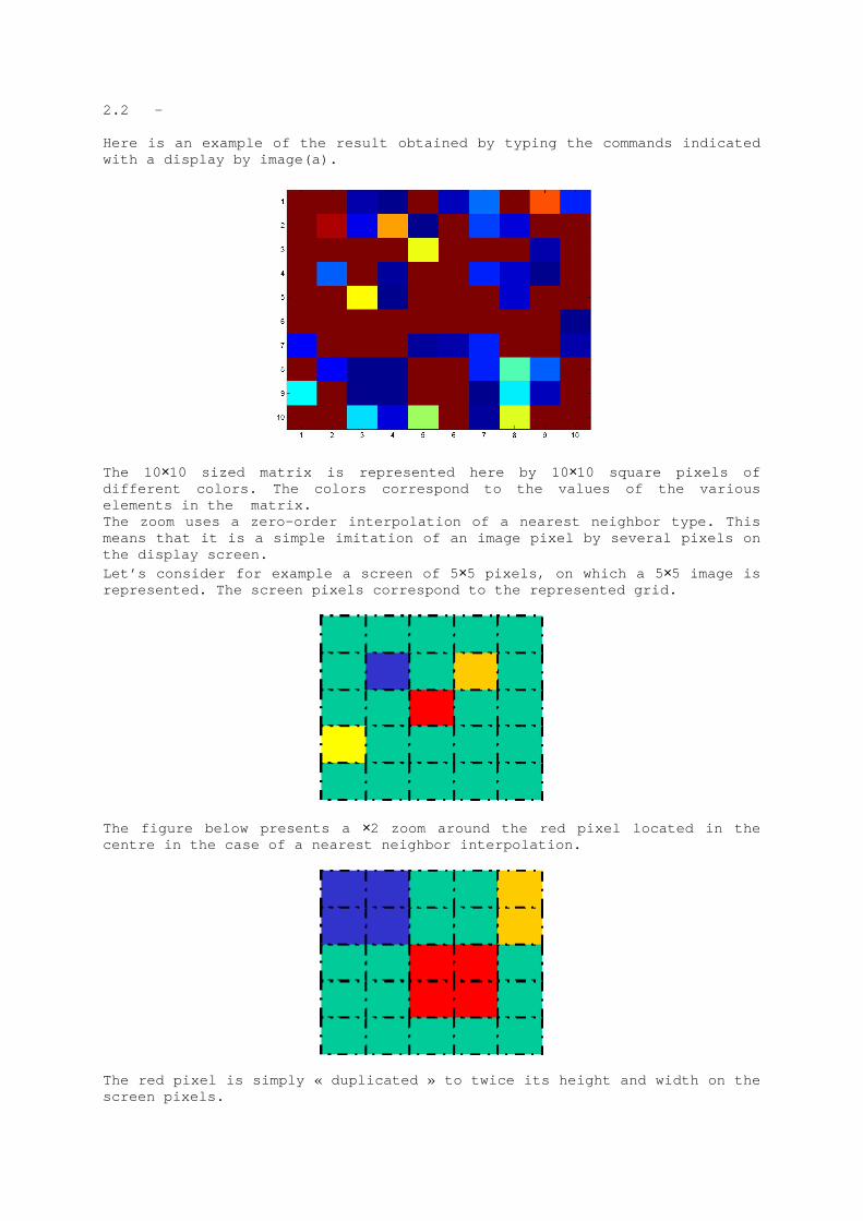
2.2 – Here is an example of the result obtained by typing the commands indicated with a display by image(a).
The 10 ×10 sized matrix is represented here by 10 ×10 square pixels of different colors. The colors correspond to the valu es of the various elements in the matrix. The zoom uses a zero-order interpolation of a neare st neighbor type. This means that it is a simple imitation of an image pix el by several pixels on the display screen. Let’s consider for example a screen of 5 ×5 pixels, on which a 5 ×5 image is represented. The screen pixels correspond to the re presented grid.
The figure below presents a ×2 zoom around the red pixel located in the centre in the case of a nearest neighbor interpolat ion.
The red pixel is simply « duplicated » to twice its height and width on the screen pixels.
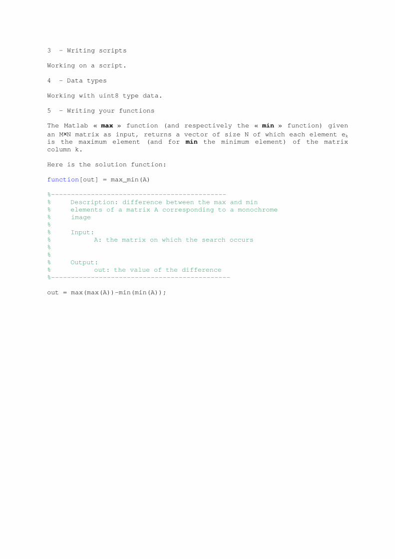
3 – Writing scripts Working on a script. 4 – Data types Working with uint8 type data. 5 – Writing your functions The Matlab « max » function (and respectively the « min » function) given
an M ×N matrix as input, returns a vector of size N of wh ich each element e k is the maximum element (and for min the minimum element) of the matrix column k. Here is the solution function: function [out] = max_min(A) %-------------------------------------------- % Description: difference between the max and min % elements of a matrix A corresponding to a monochr ome % image % % Input: % A: the matrix on which the search occurs % % % Output: % out: the value of the difference %--------------------------------------------- out = max(max(A))-min(min(A));
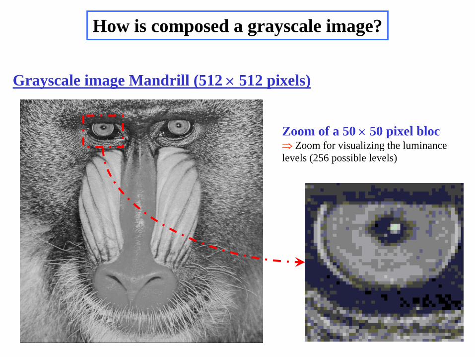
How is composed a grayscale image?
Grayscale image Mandrill (512 ×
512 pixels)
Zoom of a 50 ×
50 pixel bloc⇒ Zoom for visualizing the luminance levels (256 possible levels)
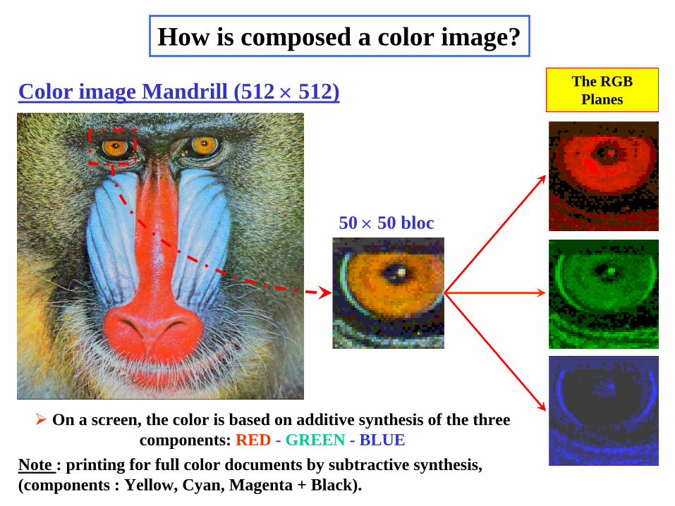
Color image Mandrill (512 ×
512)
How is composed a color image?
50 ×
50 bloc
The RGB Planes
On a screen, the color is based on additive synthesis of the three components: RED - GREEN - BLUE
Note : printing for full color documents by subtractive synthesis, (components : Yellow, Cyan, Magenta + Black).
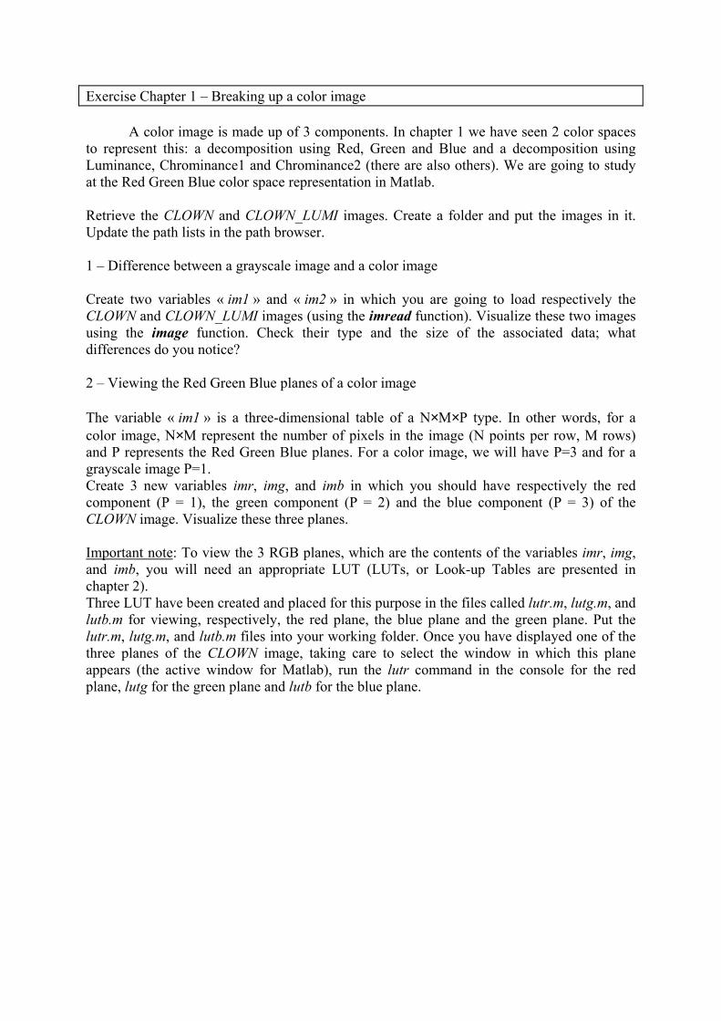
Exercise Chapter 1 – Breaking up a color image
A color image is made up of 3 components. In chapter 1 we have seen 2 color spaces
to represent this: a decomposition using Red, Green and Blue and a decomposition using
Luminance, Chrominance1 and Chrominance2 (there are also others). We are going to study
at the Red Green Blue color space representation in Matlab.
Retrieve the CLOWN and CLOWN_LUMI images. Create a folder and put the images in it.
Update the path lists in the path browser.
1 – Difference between a grayscale image and a color image
Create two variables « im1 » and « im2 » in which you are going to load respectively the
CLOWN and CLOWN_LUMI images (using the imread function). Visualize these two images
using the image function. Check their type and the size of the associated data; what
differences do you notice?
2 – Viewing the Red Green Blue planes of a color image
The variable « im1 » is a three-dimensional table of a N×M×P type. In other words, for a color image, N×M represent the number of pixels in the image (N points per row, M rows)
and P represents the Red Green Blue planes. For a color image, we will have P=3 and for a
grayscale image P=1.
Create 3 new variables imr, img, and imb in which you should have respectively the red
component (P = 1), the green component (P = 2) and the blue component (P = 3) of the
CLOWN image. Visualize these three planes.
Important note: To view the 3 RGB planes, which are the contents of the variables imr, img,
and imb, you will need an appropriate LUT (LUTs, or Look-up Tables are presented in
chapter 2).
Three LUT have been created and placed for this purpose in the files called lutr.m, lutg.m, and
lutb.m for viewing, respectively, the red plane, the blue plane and the green plane. Put the
lutr.m, lutg.m, and lutb.m files into your working folder. Once you have displayed one of the
three planes of the CLOWN image, taking care to select the window in which this plane
appears (the active window for Matlab), run the lutr command in the console for the red
plane, lutg for the green plane and lutb for the blue plane.
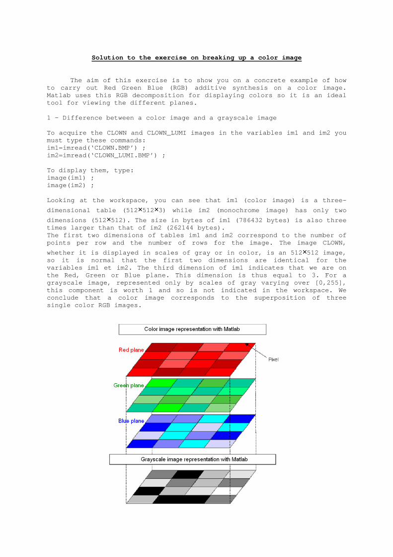
Solution to the exercise on breaking up a color image
The aim of this exercise is to show you on a concr ete example of how to carry out Red Green Blue (RGB) additive synthesi s on a color image. Matlab uses this RGB decomposition for displaying c olors so it is an ideal tool for viewing the different planes. 1 – Difference between a color image and a grayscal e image To acquire the CLOWN and CLOWN_LUMI images in the variables im1 and im2 you must type these commands: im1=imread(‘CLOWN.BMP’) ; im2=imread(‘CLOWN_LUMI.BMP’) ; To display them, type: image(im1) ; image(im2) ; Looking at the workspace, you can see that im1 (color image) is a three-
dimensional table (512 ×512×3) while im2 (monochrome image) has only two
dimensions (512 ×512). The size in bytes of im1 (786432 bytes) is also three times larger than that of im2 (262144 bytes). The first two dimensions of tables im1 and im2 correspond to the number of points per row and the number of rows for the image . The image CLOWN,
whether it is displayed in scales of gray or in col or, is an 512 ×512 image, so it is normal that the first two dimensions are i dentical for the variables im1 et im2. The third dimension of im1 indicates that we are on the Red, Green or Blue plane. This dimension is thu s equal to 3. For a grayscale image, represented only by scales of gray varying over [0,255], this component is worth 1 and so is not indicated i n the workspace. We conclude that a color image corresponds to the supe rposition of three single color RGB images.

2 – Visualizing the Red Green Blue planes of a colo r image Here is the script for acquiring the three RGB plan es in the variables imr, img, and imb: imr=im1(:,:,1); % Red plane img=im1(:,:,2); % Green plane imb=im1(:,:,3); % Blue plane Once you have imported the lutr, lutb, and lutg files into your working folder, here are the scripts for displaying the thr ee planes of the image: % Displaying the Red plane figure % Create a new window for displaying the image image(imr); lutr; % Displaying the Green plane figure image(img); lutg; % Displaying the Blue plane figure image(imb); lutb; Here are the obtained results:
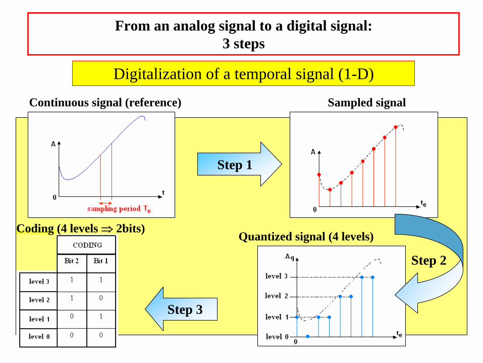
From an analog signal to a digital signal: 3 steps
Digitalization of a temporal signal (1-D)
Continuous signal (reference)
Step 1
Sampled signal
Quantized signal (4 levels)
Step 3
Step 2
Coding (4 levels ⇒ 2bits)
Quantization : the continuous signal amplitude is represented by a set of discrete values (reconstruction levels).
Sampling : the original temporal signal is represented as a set of finite values. The values are sampled with the sampling period Te.
Coding : the binary coding of the reconstruction levels uses k bits (⇒ 2k possible levels).
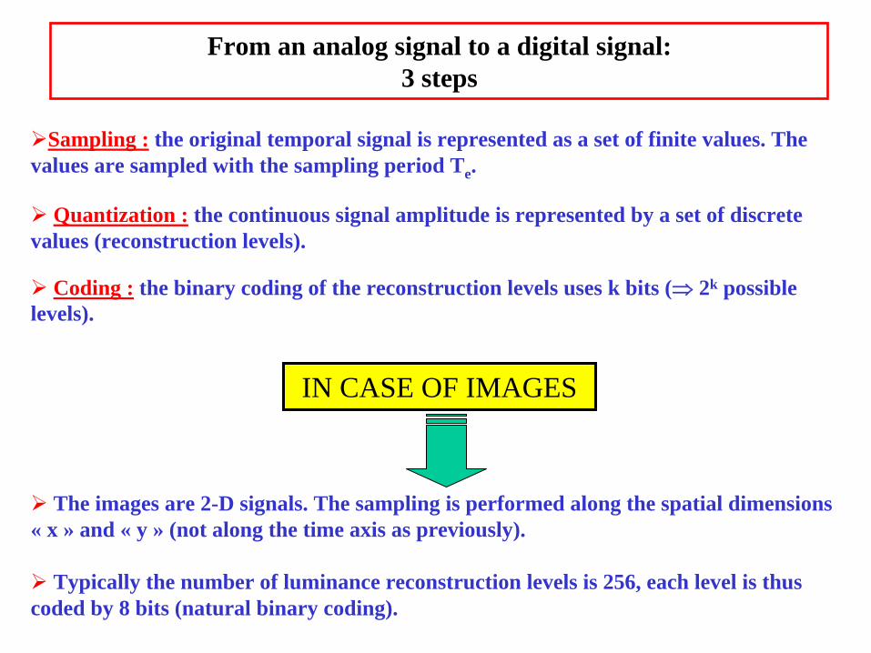
From an analog signal to a digital signal: 3 steps
IN CASE OF IMAGES
The images are 2-D signals. The sampling is performed along the spatial dimensions « x » and « y » (not along the time axis as previously).
Typically the number of luminance reconstruction levels is 256, each level is thus coded by 8 bits (natural binary coding).
2005 D. BARBA 1
Image digitalization
Sampling and Quantization
Chapter 1
MULTIMEDIA SIGNAL PROCESSING
2005 D. BARBA 2
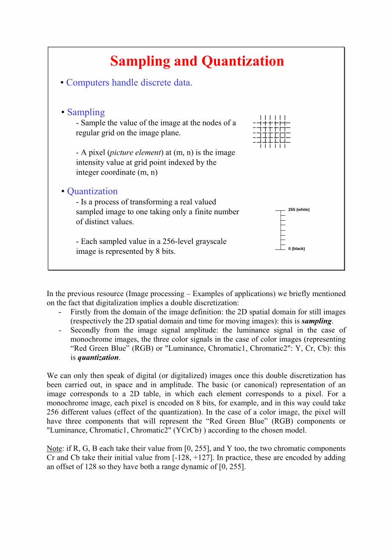
Sampling and Quantization
• Sampling- Sample the value of the image at the nodes of a
regular grid on the image plane.
- A pixel (picture element) at (m, n) is the image
intensity value at grid point indexed by the
integer coordinate (m, n)
• Quantization- Is a process of transforming a real valued
sampled image to one taking only a finite number
of distinct values.
- Each sampled value in a 256-level grayscale
image is represented by 8 bits.
• Computers handle discrete data.
255 (white)
0 (black)
In the previous resource (Image processing – Examples of applications) we briefly mentioned
on the fact that digitalization implies a double discretization:
- Firstly from the domain of the image definition: the 2D spatial domain for still images
(respectively the 2D spatial domain and time for moving images): this is sampling.
- Secondly from the image signal amplitude: the luminance signal in the case of
monochrome images, the three color signals in the case of color images (representing
“Red Green Blue” (RGB) or "Luminance, Chromatic1, Chromatic2": Y, Cr, Cb): this
is quantization.
We can only then speak of digital (or digitalized) images once this double discretization has
been carried out, in space and in amplitude. The basic (or canonical) representation of an
image corresponds to a 2D table, in which each element corresponds to a pixel. For a
monochrome image, each pixel is encoded on 8 bits, for example, and in this way could take
256 different values (effect of the quantization). In the case of a color image, the pixel will
have three components that will represent the “Red Green Blue” (RGB) components or
"Luminance, Chromatic1, Chromatic2" (YCrCb) ) according to the chosen model.
Note: if R, G, B each take their value from [0, 255], and Y too, the two chromatic components
Cr and Cb take their initial value from [-128, +127]. In practice, these are encoded by adding
an offset of 128 so they have both a range dynamic of [0, 255].
2005 D. BARBA 3
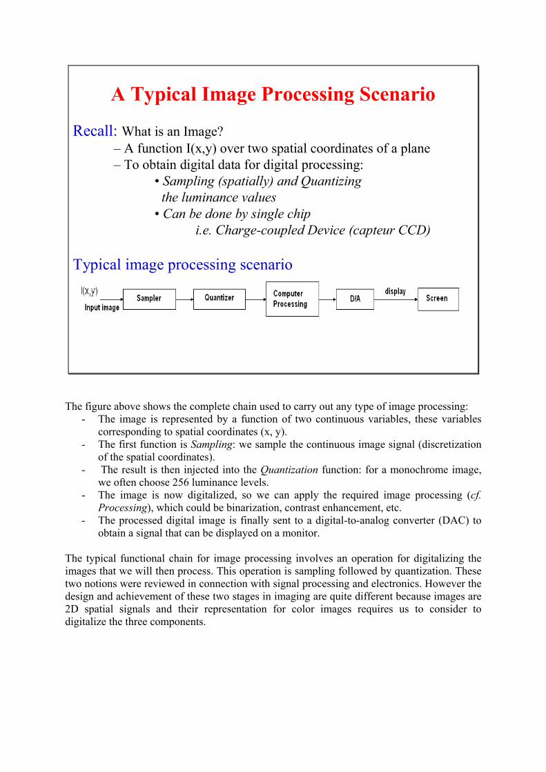
A Typical Image Processing Scenario
Recall: What is an Image?
– A function I(x,y) over two spatial coordinates of a plane
– To obtain digital data for digital processing:
• Sampling (spatially) and Quantizing
the luminance values
• Can be done by single chip
i.e. Charge-coupled Device (capteur CCD)
Typical image processing scenario
The figure above shows the complete chain used to carry out any type of image processing:
- The image is represented by a function of two continuous variables, these variables
corresponding to spatial coordinates (x, y).
- The first function is Sampling: we sample the continuous image signal (discretization
of the spatial coordinates).
- The result is then injected into the Quantization function: for a monochrome image,
we often choose 256 luminance levels.
- The image is now digitalized, so we can apply the required image processing (cf.
Processing), which could be binarization, contrast enhancement, etc.
- The processed digital image is finally sent to a digital-to-analog converter (DAC) to
obtain a signal that can be displayed on a monitor.
The typical functional chain for image processing involves an operation for digitalizing the
images that we will then process. This operation is sampling followed by quantization. These
two notions were reviewed in connection with signal processing and electronics. However the
design and achievement of these two stages in imaging are quite different because images are
2D spatial signals and their representation for color images requires us to consider to
digitalize the three components.
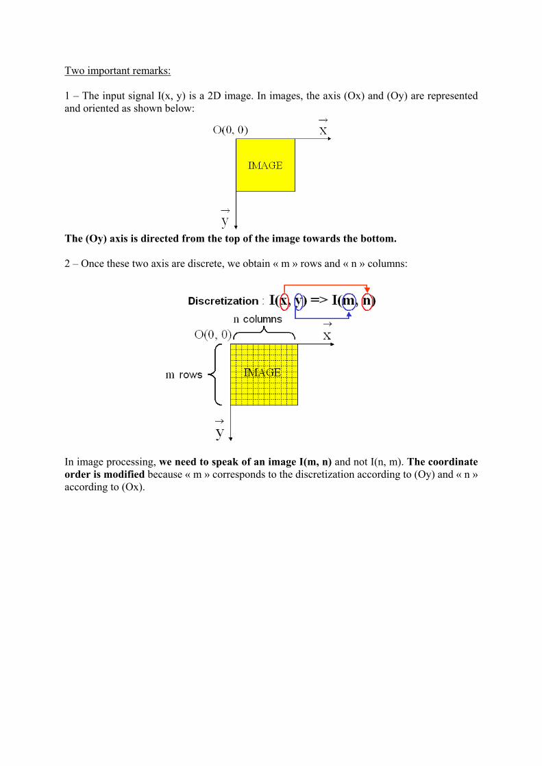
Two important remarks:
1 – The input signal I(x, y) is a 2D image. In images, the axis (Ox) and (Oy) are represented
and oriented as shown below:
The (Oy) axis is directed from the top of the image towards the bottom.
2 – Once these two axis are discrete, we obtain « m » rows and « n » columns:
In image processing, we need to speak of an image I(m, n) and not I(n, m). The coordinate
order is modified because « m » corresponds to the discretization according to (Oy) and « n »
according to (Ox).
2005 D. BARBA 4
Recall: 1-D Sampling
• Time domain
- Multiply continuous-time signal with periodic impulse train
• Frequency domain- Duality: sampling in one domain � tiling in another domain
� the Fourier Transform of an impulse train is an impulse train (proper
scaling & stretching)
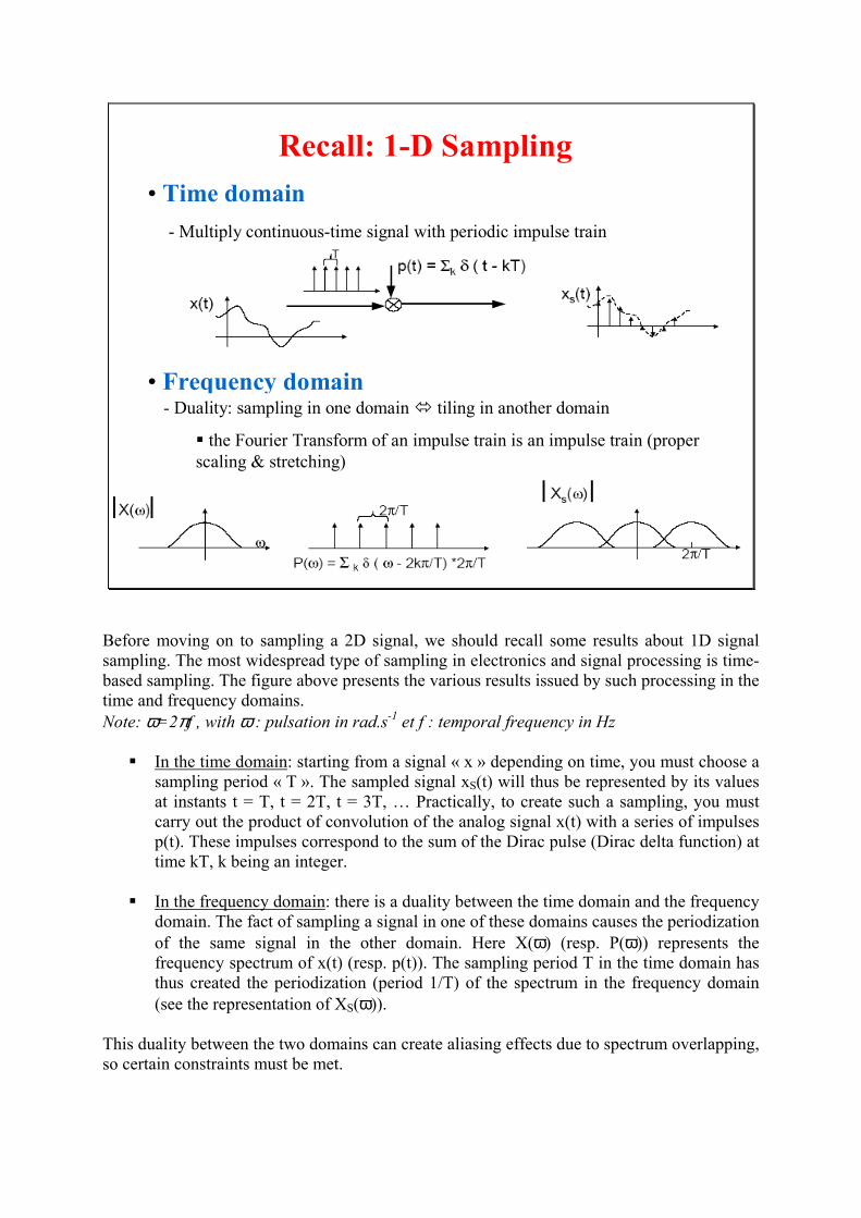
Before moving on to sampling a 2D signal, we should recall some results about 1D signal
sampling. The most widespread type of sampling in electronics and signal processing is time-
based sampling. The figure above presents the various results issued by such processing in the
time and frequency domains.
Note: ω=2πf , with ω : pulsation in rad.s-1 et f : temporal frequency in Hz
� In the time domain: starting from a signal « x » depending on time, you must choose a
sampling period « T ». The sampled signal xS(t) will thus be represented by its values
at instants t = T, t = 2T, t = 3T, … Practically, to create such a sampling, you must
carry out the product of convolution of the analog signal x(t) with a series of impulses
p(t). These impulses correspond to the sum of the Dirac pulse (Dirac delta function) at
time kT, k being an integer.
� In the frequency domain: there is a duality between the time domain and the frequency
domain. The fact of sampling a signal in one of these domains causes the periodization
of the same signal in the other domain. Here X(ω) (resp. P(ω)) represents the
frequency spectrum of x(t) (resp. p(t)). The sampling period T in the time domain has
thus created the periodization (period 1/T) of the spectrum in the frequency domain
(see the representation of XS(ω)).
This duality between the two domains can create aliasing effects due to spectrum overlapping,
so certain constraints must be met.
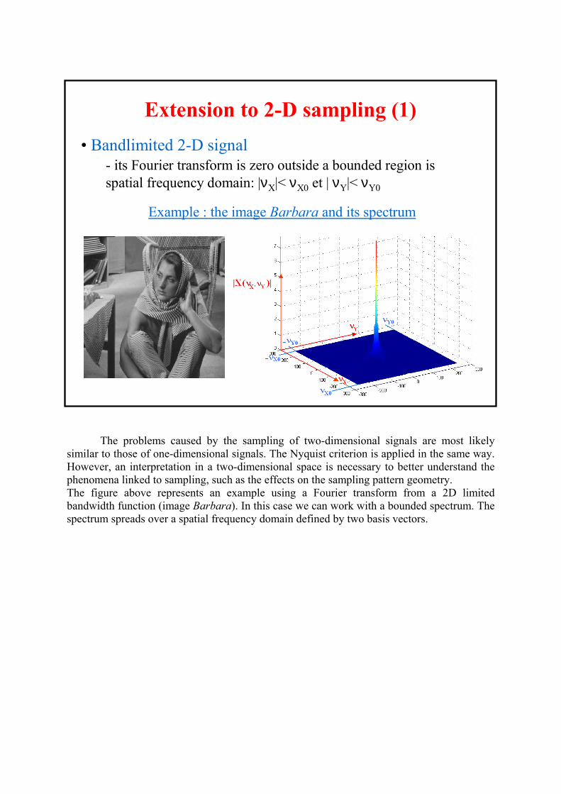
The problems caused by the sampling of two-dimensional signals are most likely
similar to those of one-dimensional signals. The Nyquist criterion is applied in the same way.
However, an interpretation in a two-dimensional space is necessary to better understand the
phenomena linked to sampling, such as the effects on the sampling pattern geometry.
The figure above represents an example using a Fourier transform from a 2D limited
bandwidth function (image Barbara). In this case we can work with a bounded spectrum. The
spectrum spreads over a spatial frequency domain defined by two basis vectors.
2005 D. BARBA 7
Extension to 2-D sampling (1)
• Bandlimited 2-D signal
- its Fourier transform is zero outside a bounded region is
spatial frequency domain: |νX|< νX0 et | νY|< νY0
Example : the image Barbara and its spectrum
2005 D. BARBA 8
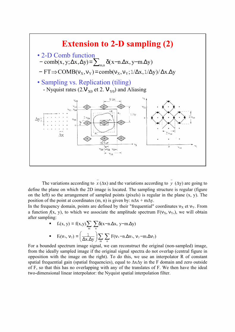
Extension to 2-D sampling (2)
• 2-D Comb function
• Sampling vs. Replication (tiling)- Nyquist rates (2.νX0 et 2. νY0) and Aliasing
)y.my,x.nx()y,x;y,x(combn,m
∆−∆−δ=∆∆− ∑y.x/)y/,x/;,(comb),(COMBFT YXYX ∆∆∆∆νν=νν⇒− 11
The variations according to →x (∆x) and the variations according to
→y (∆y) are going to
define the plane on which the 2D image is located. The sampling structure is regular (figure
on the left) so the arrangement of sampled points (pixels) is regular in the plane (x, y). The
position of the point at coordinates (m, n) is given by: n∆x + m∆y.
In the frequency domain, points are defined by their "frequential" coordinates νX et νY. From
a function f(x, y), to which we associate the amplitude spectrum F(νX, νY,), we will obtain
after sampling:
� ∑ ∑ ∆−∆−δ=m n
e )y.my,x.nx().y,x(f)y,x(f
� ∑∑ ν∆−νν∆−ν
∆∆=νν
m n
yyxxyxe ).m,.n(Fy.x
),(F 1
For a bounded spectrum image signal, we can reconstruct the original (non-sampled) image,
from the ideally sampled image if the original signal spectra do not overlap (central figure in
opposition with the image on the right). To do this, we use an interpolator R of constant
spatial frequential gain (spatial frequencies), equal to ∆x∆y in the F domain and zero outside
of F, so that this has no overlapping with any of the translates of F. We then have the ideal
two-dimensional linear interpolator: the Nyquist spatial interpolation filter.
2005 D. BARBA 9
Sampling Lattice in Color Images and Videos
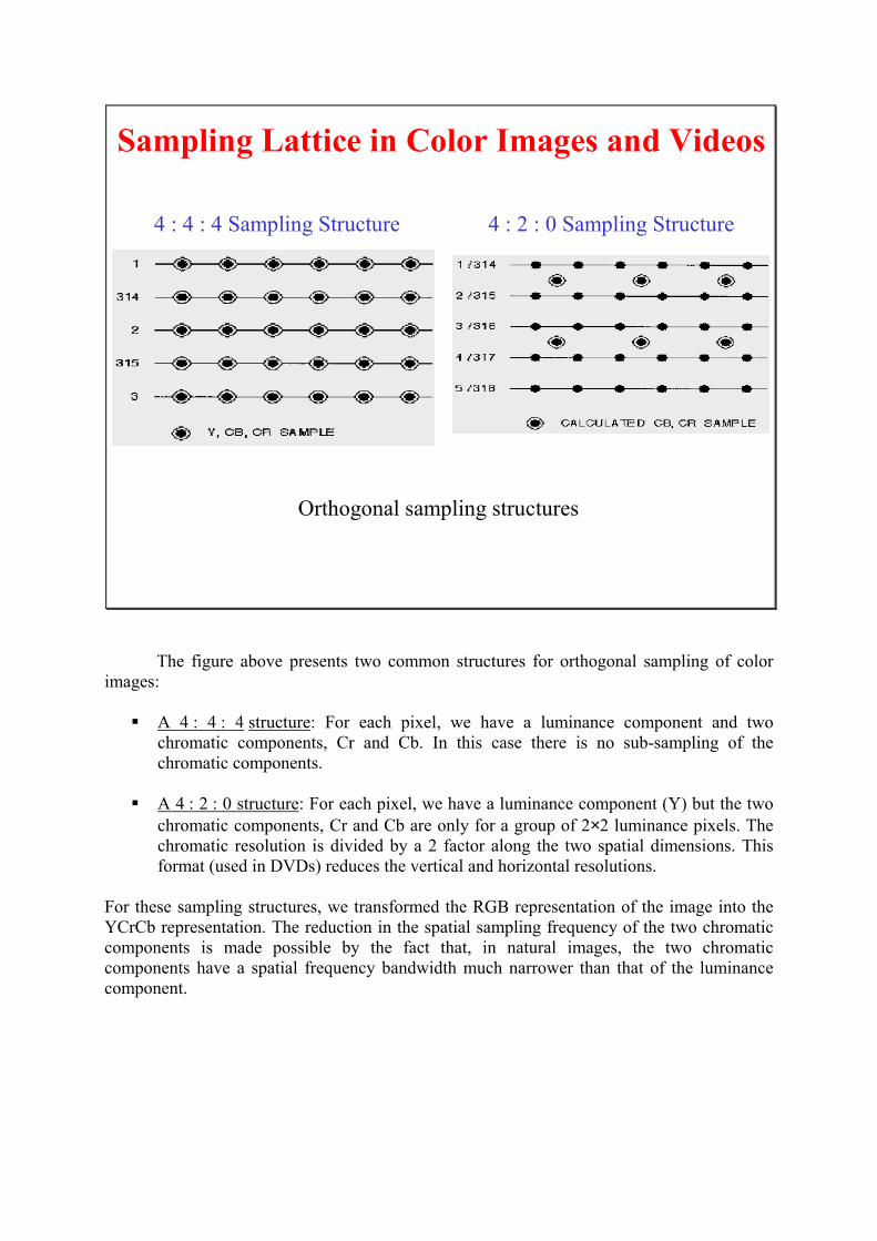
4 : 4 : 4 Sampling Structure 4 : 2 : 0 Sampling Structure
Orthogonal sampling structures
The figure above presents two common structures for orthogonal sampling of color
images:
� A 4 : 4 : 4 structure: For each pixel, we have a luminance component and two
chromatic components, Cr and Cb. In this case there is no sub-sampling of the
chromatic components.
� A 4 : 2 : 0 structure: For each pixel, we have a luminance component (Y) but the two
chromatic components, Cr and Cb are only for a group of 2×2 luminance pixels. The
chromatic resolution is divided by a 2 factor along the two spatial dimensions. This
format (used in DVDs) reduces the vertical and horizontal resolutions.
For these sampling structures, we transformed the RGB representation of the image into the
YCrCb representation. The reduction in the spatial sampling frequency of the two chromatic
components is made possible by the fact that, in natural images, the two chromatic
components have a spatial frequency bandwidth much narrower than that of the luminance
component.
2005 D. BARBA 10
Examples of image Sampling
(with zero-order interpolator)
Original Sampling
4 × 4 downsampling
16 × 16 downsamplingImage Lena
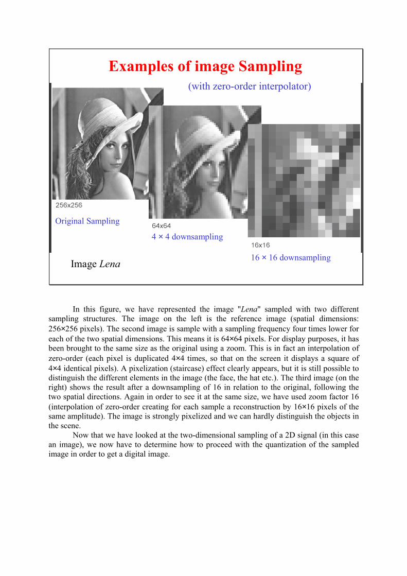
In this figure, we have represented the image "Lena" sampled with two different
sampling structures. The image on the left is the reference image (spatial dimensions:
256×256 pixels). The second image is sample with a sampling frequency four times lower for
each of the two spatial dimensions. This means it is 64×64 pixels. For display purposes, it has
been brought to the same size as the original using a zoom. This is in fact an interpolation of
zero-order (each pixel is duplicated 4×4 times, so that on the screen it displays a square of
4×4 identical pixels). A pixelization (staircase) effect clearly appears, but it is still possible to
distinguish the different elements in the image (the face, the hat etc.). The third image (on the
right) shows the result after a downsampling of 16 in relation to the original, following the
two spatial directions. Again in order to see it at the same size, we have used zoom factor 16
(interpolation of zero-order creating for each sample a reconstruction by 16×16 pixels of the
same amplitude). The image is strongly pixelized and we can hardly distinguish the objects in
the scene.
Now that we have looked at the two-dimensional sampling of a 2D signal (in this case
an image), we now have to determine how to proceed with the quantization of the sampled
image in order to get a digital image.

2005 D. BARBA 11
Quantization
Video and Image digitalization
2005 D. BARBA 12
Quantization
• Scalar quantization
xQuantization
y = Q(x)
continuous
X
Y
t0 t1
r0
ti-1 ti ti+1 tK-1 tK
ri-1 ri rK-1
Decision thresholds
Reconstruction level
• Quantization functionfor tj ≤ x < t j+1 then y = rj ∀j = 0, …, K-1
and t0= x min ; tK = x max
discrete
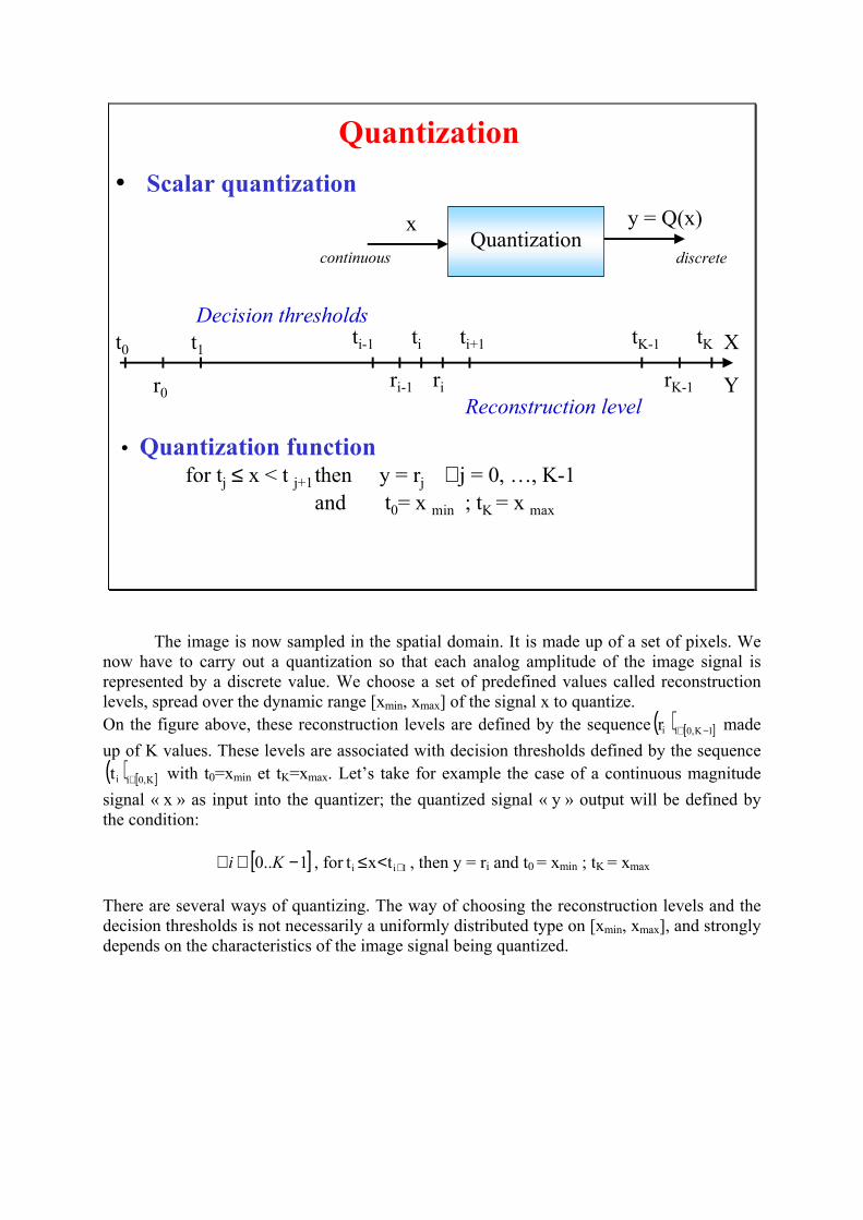
The image is now sampled in the spatial domain. It is made up of a set of pixels. We
now have to carry out a quantization so that each analog amplitude of the image signal is
represented by a discrete value. We choose a set of predefined values called reconstruction
levels, spread over the dynamic range [xmin, xmax] of the signal x to quantize.
On the figure above, these reconstruction levels are defined by the sequence ( ) [ ]1K,0iir −∈ made
up of K values. These levels are associated with decision thresholds defined by the sequence
( ) [ ]K,0iit ∈ with t0=xmin et tK=xmax. Let’s take for example the case of a continuous magnitude
signal « x » as input into the quantizer; the quantized signal « y » output will be defined by
the condition:
[ ]1..0 −∈∀ Ki , for 1ii txt +<≤ , then y = ri and t0 = xmin ; tK = xmax
There are several ways of quantizing. The way of choosing the reconstruction levels and the
decision thresholds is not necessarily a uniformly distributed type on [xmin, xmax], and strongly
depends on the characteristics of the image signal being quantized.
2005 D. BARBA 13
Example of a quantization law
- Multiple-to-one mapping
- Want to minimize error
•Mean-square-error (ε)
- Let an input « u » with the
probability density function pu(x)
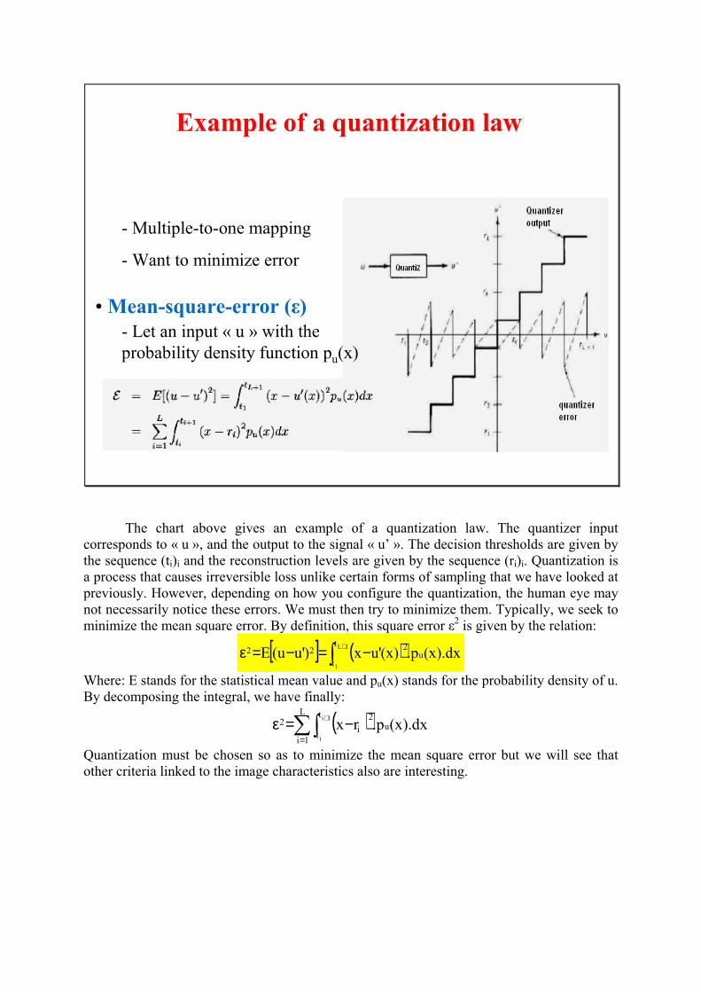
The chart above gives an example of a quantization law. The quantizer input
corresponds to « u », and the output to the signal « u’ ». The decision thresholds are given by
the sequence (ti)i and the reconstruction levels are given by the sequence (ri)i. Quantization is
a process that causes irreversible loss unlike certain forms of sampling that we have looked at
previously. However, depending on how you configure the quantization, the human eye may
not necessarily notice these errors. We must then try to minimize them. Typically, we seek to
minimize the mean square error. By definition, this square error ε2 is given by the relation:
[ ] ( )∫+ −=−=ε 1L
1
t
tu
222 dx).x(p.)x('ux)'uu(E
Where: E stands for the statistical mean value and pu(x) stands for the probability density of u.
By decomposing the integral, we have finally:
( )∑∫=
+ −=εL
1i
t
tu
2
i2
1i
i
dx).x(p.rx
Quantization must be chosen so as to minimize the mean square error but we will see that
other criteria linked to the image characteristics also are interesting.
2005 D. BARBA 14
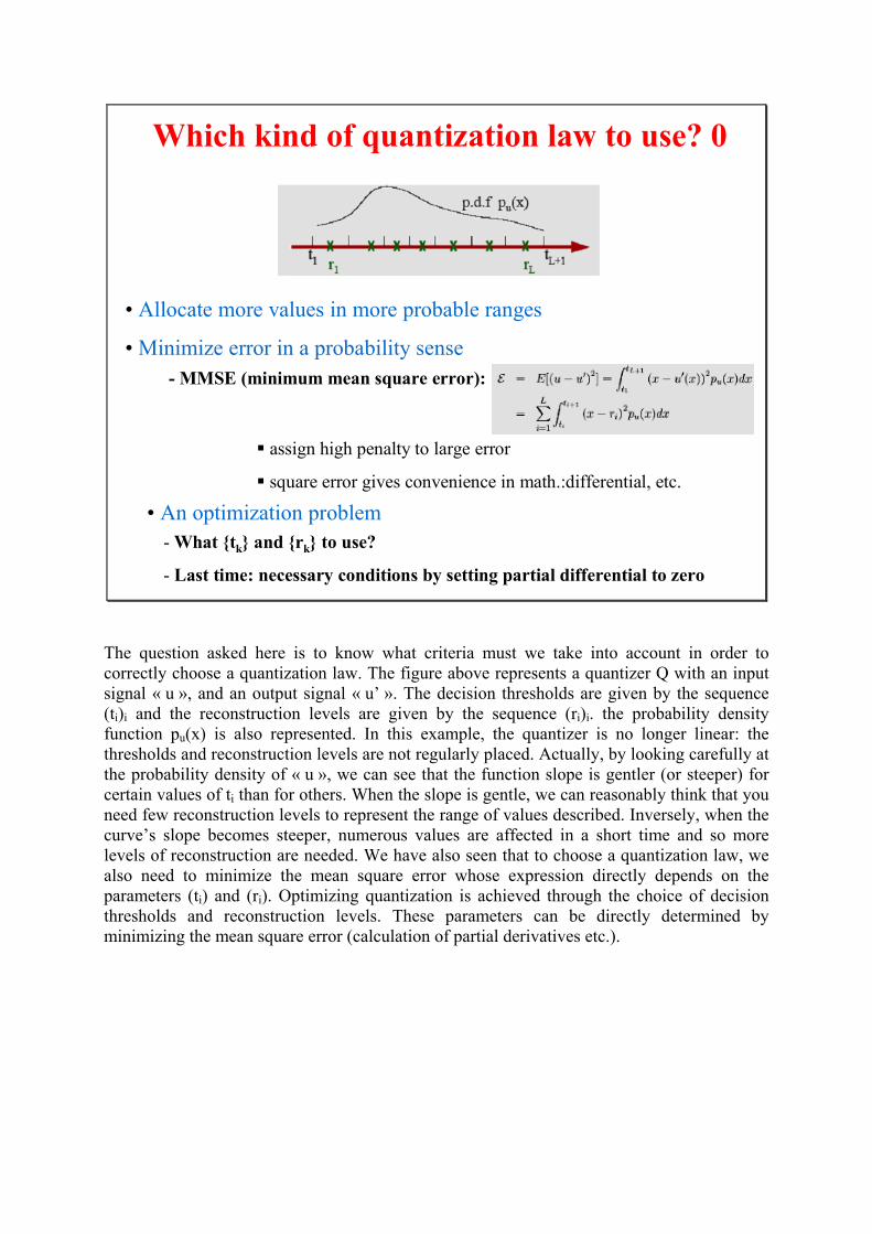
• Allocate more values in more probable ranges
• Minimize error in a probability sense
- MMSE (minimum mean square error):
� assign high penalty to large error
� square error gives convenience in math.:differential, etc.
• An optimization problem
-What {tk} and {rk} to use?
- Last time: necessary conditions by setting partial differential to zero
Which kind of quantization law to use? 0
The question asked here is to know what criteria must we take into account in order to
correctly choose a quantization law. The figure above represents a quantizer Q with an input
signal « u », and an output signal « u’ ». The decision thresholds are given by the sequence
(ti)i and the reconstruction levels are given by the sequence (ri)i. the probability density
function pu(x) is also represented. In this example, the quantizer is no longer linear: the
thresholds and reconstruction levels are not regularly placed. Actually, by looking carefully at
the probability density of « u », we can see that the function slope is gentler (or steeper) for
certain values of ti than for others. When the slope is gentle, we can reasonably think that you
need few reconstruction levels to represent the range of values described. Inversely, when the
curve’s slope becomes steeper, numerous values are affected in a short time and so more
levels of reconstruction are needed. We have also seen that to choose a quantization law, we
also need to minimize the mean square error whose expression directly depends on the
parameters (ti) and (ri). Optimizing quantization is achieved through the choice of decision
thresholds and reconstruction levels. These parameters can be directly determined by
minimizing the mean square error (calculation of partial derivatives etc.).
2005 D. BARBA 15
Optimal Quantization (1)
• Criteria of optimal quantization
– Mean Square Error ( y = Q(x) )
ε2 = E { ( X-Y)2 } = ∫-∞ (x-y)2 px(x) dx
ε2 = ∑i ∫ (x-yi)2 px(x) dx
ti+1 = (r i+ r i+1) / 2
minimization of ε2: ri= E {X / x∈[ ti , ti+1 ] }
ti+1
+∞
r0
X
Y
t0 t1ti-1 ti ti+1 tK-1 tK
ri-1 ri rK-1
ti
• Special case: uniform probability density function: px(x) is constant
then ti+1 = (r i+ r i+1) / 2 and ri = (t i+ t i+1) / 2
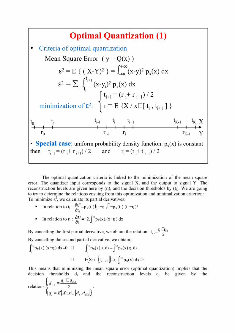
The optimal quantization criteria is linked to the minimization of the mean square
error. The quantizer input corresponds to the signal X, and the output to signal Y. The
reconstruction levels are given here by (ri), and the decision thresholds by (ti). We are going
to try to determine the relations ensuing from this optimization and minimalization criterion:
To minimize ε2, we calculate its partial derivatives:
� In relation to ti : ( ) )²rt).(t(prt).t(pt²
iiiX
2
1iiiX
i
−−−=∂ε∂
−
� In relation to ri : ∫+ −−=
∂ε∂ 1i
i
t
tiX
i
dx).rx).(x(p.2r²
By cancelling the first partial derivative, we obtain the relation: 2rr
t 1ii1i
++=+
By cancelling the second partial derivative, we obtain:
0dx).rx).(x(p1i
i
t
tiX =−∫
+ ⇔ ∫∫
++ = 1i
i
1i
i
t
tiX
t
tX dx.r).x(pdx.x).x(p
⇔ [ [{ } i
t
tXi1ii rdx).x(p.rt,tx;XE
1i
i
==∈ ∫+
+
This means that minimizing the mean square error (optimal quantization) implies that the
decision thresholds di and the reconstruction levels qi be given by the
relations:
[ [{ }
∈=
+=
+
++
1
1
1
,;
2
iii
ii
i
ddxXEq
qqd
.
These are the two relations obtained by Max. These show that the optimal quantizer for a
signal using a non-uniform probability density function is not a linear quantizer.
In the particular case of an input signal whose probability density is constant over [xmin, xmax],
we have :)(
1)(
minmax xxxpX −
= , and we obtain the relations:
+=
+=
++
+
2rr
t
2tt
r
1ii1i
1iii
The optimal quantizer is linear in this case:K
xx∆t minmax
i
−= .
For a signal normalized over [0, 1], the minimized square error is worth: 2
2
.12
1
K=ε .
We have seen that, in order to optimize the quantizer, we must minimize the mean square
error of quantization with this criterion. Naturally, other criteria may be used, in particular
those concerning the visual appearance.
2005 D. BARBA 16
• Maximum entropy quantization : H(Y) maximum si Y est
à loi de probabilité constante
pi = ∫ px(x) dx = constant ∀i =1, ….. , K
Optimal Quantization (2)
ti
• Psycho-visual quantization of images
- Perception of small stimuli on a background: ∆L / L = cst
- Cst ≅ 0.01 in luminance TV range (given by Weber law)
« Log »Linear
Quantization
x y = Q’(x’) = Q(x)x’
X ’ X
X
ti+1
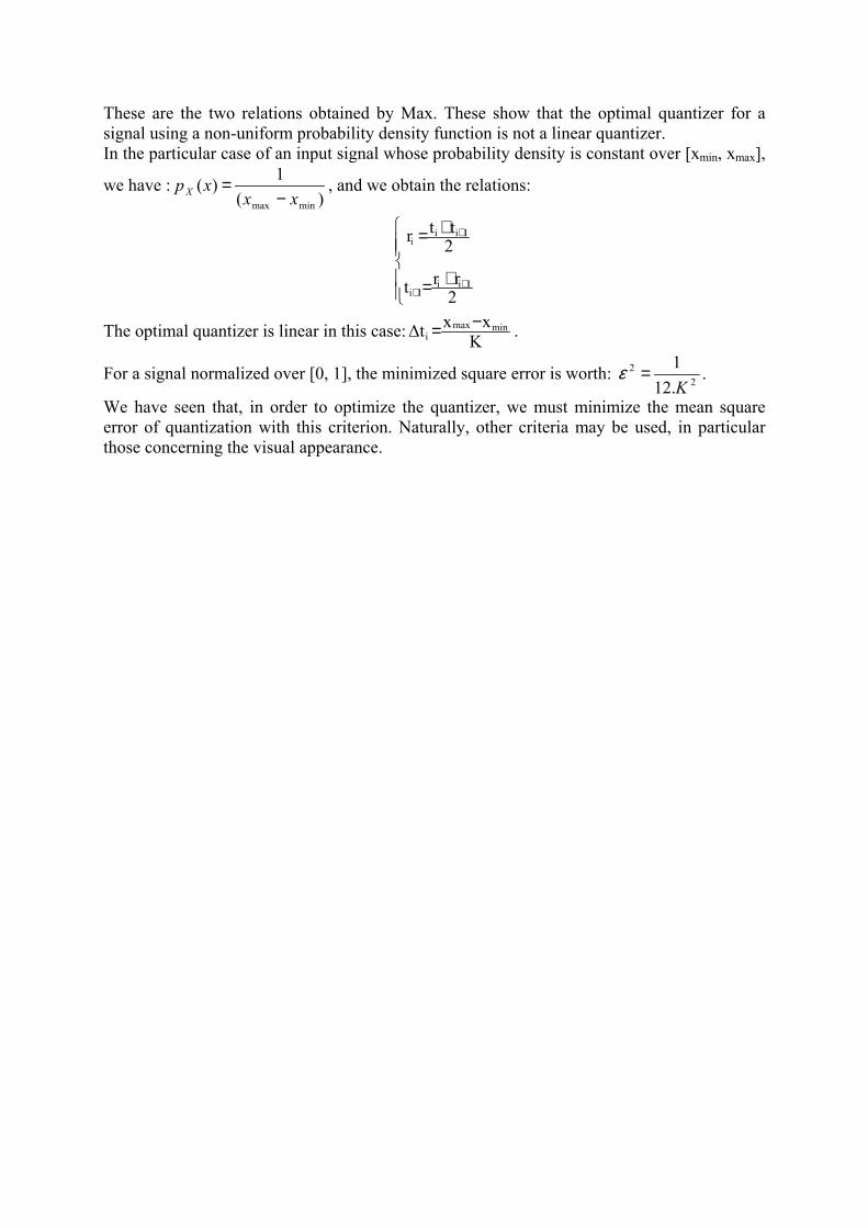
The characteristics of the human system of vision can be used to design the
quantization law. For a usual stimulus of a given form and fixed ∆L amplitude, the visibility
threshold ∆L / L is more or less constant (L being the luminance). In the TV luminance range,
it varies slightly when L goes from black to white. For a quantization at the visibility
threshold, we would have ri+1-ri=∆L. It becomes possible to use a uniform quantization on a
compressed signal by a non-linearity « f » (see diagram above). You would of course need to
carry out the reverse operation coming out of the quantizer with an expansion function.
This non-linear compression function is defined by )/(.).()( 00
LxLogdxxLxfx
Lλ≈∆= ∫ . For
television, compression « f » is already used: it is the gamma correction given by γ1
)( xxf =
that compensates for the non-linear nature of CRT-type TV screens. We then apply a linear
quantization over 256 leveks. In color television, we usually quantize the luminance and
chromatic signals separately. From a perceptual point of view, the YCrCb space is more
uniform than the RGB space.
We can see by looking at television-type applications that despite the interesting properties of
the optimal quantizer, it can sometimes be a better idea to use a non-linear compression
function and then to use a linear quantization (even if the signal’s probability density function
is not uniform). The "compression function – quantization – expansion function" series would
be chosen in order to approximate the optimal quantization law.
2005 D. BARBA 18
Example: quantization of an image
256 – level
quantization
16 - level quantization
4 - level quantizationImage Lena
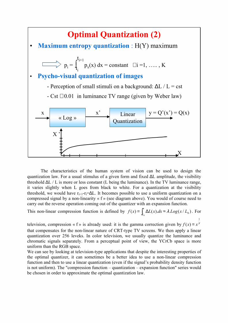
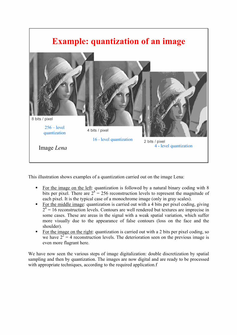
This illustration shows examples of a quantization carried out on the image Lena:
� For the image on the left: quantization is followed by a natural binary coding with 8
bits per pixel. There are 28 = 256 reconstruction levels to represent the magnitude of
each pixel. It is the typical case of a monochrome image (only in gray scales).
� For the middle image: quantization is carried out with a 4 bits per pixel coding, giving
24 = 16 reconstruction levels. Contours are well rendered but textures are imprecise in
some cases. These are areas in the signal with a weak spatial variation, which suffer
more visually due to the appearance of false contours (loss on the face and the
shoulder).
� For the image on the right: quantization is carried out with a 2 bits per pixel coding, so
we have 22 = 4 reconstruction levels. The deterioration seen on the previous image is
even more flagrant here.
We have now seen the various steps of image digitalization: double discretization by spatial
sampling and then by quantization. The images are now digital and are ready to be processed
with appropriate techniques, according to the required application.f
Chapter 1 – Introduction to digital image processing
TEST
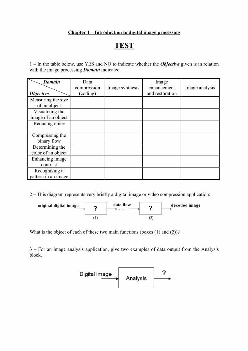
1 – In the table below, use YES and NO to indicate whether the Objective given is in relation
with the image processing Domain indicated.
Domain
Objective
Data
compression
(coding)
Image synthesis
Image
enhancement
and restoration
Image analysis
Measuring the size
of an object
Visualizing the
image of an object
Reducing noise
Compressing the
binary flow
Determining the
color of an object
Enhancing image
contrast
Recognizing a
pattern in an image
2 – This diagram represents very briefly a digital image or video compression application:
What is the object of each of these two main functions (boxes (1) and (2))?
3 – For an image analysis application, give two examples of data output from the Analysis
block.
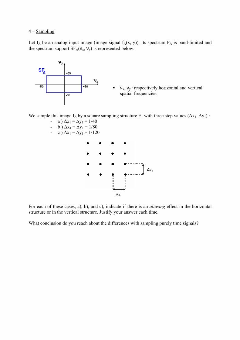
4 – Sampling
Let IA be an analog input image (image signal fA(x, y)). Its spectrum FA is band-limited and
the spectrum support SFA(νx, νy) is represented below:
� νx, νy : respectively horizontal and vertical
spatial frequencies.
We sample this image IA by a square sampling structure E1 with three step values (∆x1, ∆y1) :
- a ) ∆x1 = ∆y1 = 1/40
- b ) ∆x1 = ∆y1 = 1/80
- c ) ∆x1 = ∆y1 = 1/120
For each of these cases, a), b), and c), indicate if there is an aliasing effect in the horizontal
structure or in the vertical structure. Justify your answer each time.
What conclusion do you reach about the differences with sampling purely time signals?
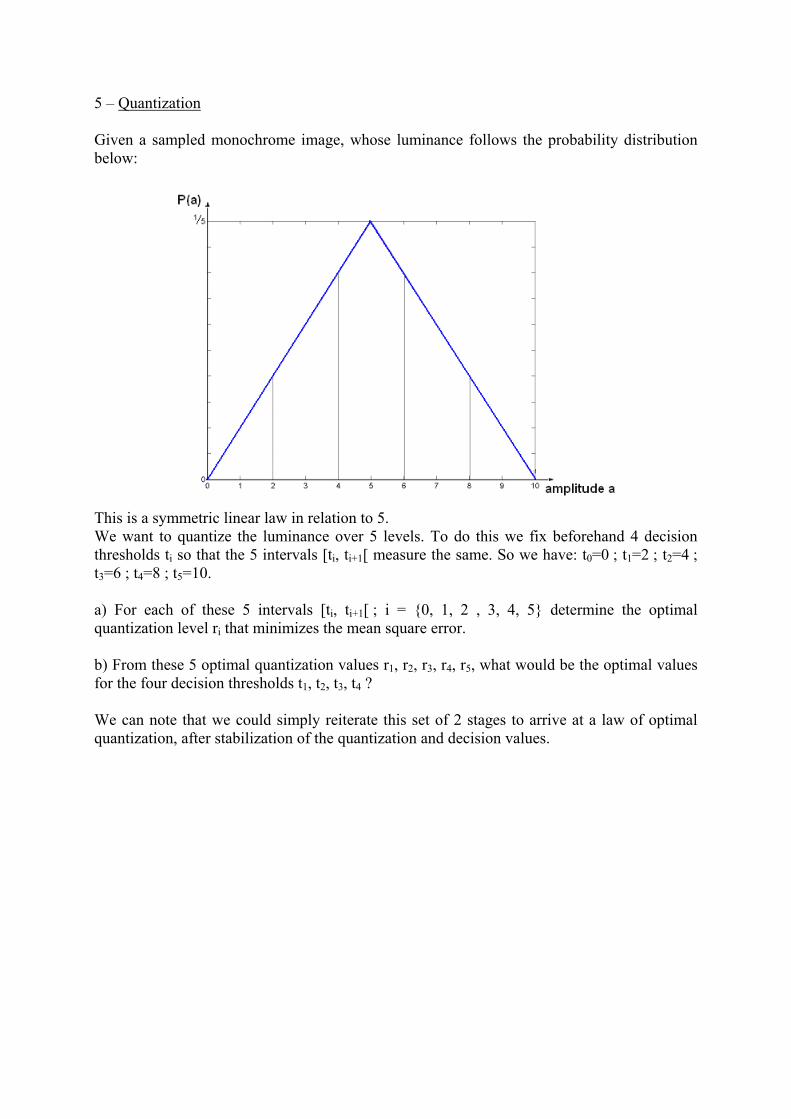
5 – Quantization
Given a sampled monochrome image, whose luminance follows the probability distribution
below:
This is a symmetric linear law in relation to 5.
We want to quantize the luminance over 5 levels. To do this we fix beforehand 4 decision
thresholds ti so that the 5 intervals [ti, ti+1[ measure the same. So we have: t0=0 ; t1=2 ; t2=4 ;
t3=6 ; t4=8 ; t5=10.
a) For each of these 5 intervals [ti, ti+1[ ; i = {0, 1, 2 , 3, 4, 5} determine the optimal
quantization level ri that minimizes the mean square error.
b) From these 5 optimal quantization values r1, r2, r3, r4, r5, what would be the optimal values
for the four decision thresholds t1, t2, t3, t4 ?
We can note that we could simply reiterate this set of 2 stages to arrive at a law of optimal
quantization, after stabilization of the quantization and decision values.


![ECE-V-DIGITAL SIGNAL PROCESSING [10EC52] …vtusolution.in/.../digital-signal-processing-10ec52.pdfDigital vtusolution.in Signal Processing 10EC52 TEXT BOOK: 1. DIGITAL SIGNAL PROCESSING](https://static.documents.pub/doc/80x56/5afe42bb7f8b9a256b8ccd2e/ece-v-digital-signal-processing-10ec52-signal-processing-10ec52-text-book.jpg)


