Bachelor Thesis Project

Multimodal Summarization and Beyond

DISSERTATION SUBMITTED IN PARTIAL FULFILLMENT OF THE REQUIREMENT FOR THE DEGREE OF B.E (INFORMATION

TECHNOLOGY)

SUBMITTED BY:

Aman Khullar (708/IT/15)

GUIDED BY:

Dr. Deepika Kukreja

(Assistant Professor, Division of Information Technology)

DIVISION OF INFORMATION TECHNOLOGY NETAJI SUBHAS INSTITUTE OF TECHNOLOGY

UNIVERSITY OF DELHI2019

नताजी सभाष परौदयोिगकी ससथान NETAJI SUBHAS INSTITUTE OF TECHNOLOGY (An Institution of Govt. of NCT of Delhi-Formerly, Delhi Institute of Technology)

Azad Hind Fauj Marg, Sector-3, Dwarka, New Delhi - 110078 Telephone : 25099050; Fax : 25099025, 25099022 Website : http://www.nsit.ac.in

CERTIFICATE

This is to certify that the project titled “Multimodal Summarization and Beyond” is the bonafide work carried out by Aman Khullar (708/IT/15) student of B.E. (Information Technology) of Netaji Subhas Institute of Technology, Delhi (University of Delhi) in partial fulfillment of the requirements for the Bachelor Thesis Project (BTP) in the period of January 2019 to May 2019 of Bachelor of Engineering Information Technology.

Dr. Deepika Kukreja

Assistant Professor Division of Information Technology Netaji Subhas Institute of Technology New Delhi

Date :

Declaration This is to certify that the work which is hereby being presented by me in this project titled “Multimodal Summarization and Beyond” in partial fulfillment of the award of the degree of Bachelor of Engineering submitted to the Division of Information Technology, Netaji Subhas Institute of Technology Delhi, is a genuine account of my work carried out during the period from January 2019 to May 2019 under the guidance of Dr. Deepika Kukreja, Division of Information Technology, Netaji Subhas Institute of Technology, Delhi.

The matter embodied in the project report to the best of our knowledge has not been submitted for the award of any other degree elsewhere.

Aman Khullar (708/IT/15)

Date :

ABSTRACT The field of computer science was revolutionized in the year 1950 by a simple question posed by A.M. Turing, “Can machines think” and thought about the ‘imitation game’. Since then the field of Artificial Intelligence has undergone several revolutionary reforms supported by the exponential hardware growth and improvement in the computation power. However giving machines the power to understand human language and allow it to generate required response is still a non trivial task. This thesis tackles the problem of multimodal summarization which is defined as the task of generating output summary taking into account the different multimedia data as input. The output summary may be presented in single modality or multiple modalities.

In this thesis, the foundations of natural language processing in general and multimodal summarization in specific have been explored. Since the field of Multimodal Summarization encompasses the textual, audio and visual dataset, the foundations of these modalities have been explored and further built upon. The baseline models have been implemented on our own dataset and the widely available dataset to explore the existent state of the art techniques.

The last part of this thesis presents the novel work of this thesis, the MultiModal Bidirectional Attention Flow Model (MMBiDAF). The architecture of the model has been carefully built to integrate all the modalities and draw similarity between them to carefully generate the text which is attentive of both image and audio which further receives an attention layer to select from the audio-aware or the image-aware text. The model is then able to generate a summary by extracting the most important sentences from the given source text. The results of the model have shown to outperform the existing state of the art models in the literature.

The thesis finally concludes by giving scope of the possible future work to further improve upon this model and achieve results to infinity and beyond!

Contents1. Introduction 1

Multimodal Summarization : Foundations

2. Automatic Text Summarization 2 2.1 History 5

2.1.1 Early Approaches 5 2.1.1.1 Identifying Important Sentences 5 2.1.1.2 TF * IDF Weighting 5 2.1.1.3 Graph Based Methods 6 2.1.1.4 Degree Centrality 6 2.1.1.5 Lex Rank 6 2.1.2 Machine Learning Approaches 7 2.1.2.1 Naive-Bayes Methods 7 2.1.2.2 Hidden Markov Model 8 2.1.3 A Resurgence : Deep Learning Era 8 2.1.3.1 Recurrent Neural Networks 9 2.1.3.2 Long Short Term Memory 11 2.1.3.3 Encoder-Decoder Architecture with Attention 12 2.2 Task Definition 15 2.2.1 Problem Formulation 15 2.2.2 Evaluation 15 2.2.2.1 Recall and Precision 15 2.2.2.2 ROUGE 16 2.3 Datasets and Models 16 2.3.1 CNN/Daily Mail Dataset 16 2.3.2 Pointer Generator Networks Model 16 2.3.3 Implementation Details of Pointer Generator Networks 18

3. Speech Recognition 20 3.1 History 20

3.1.1 Early Approaches 20 3.1.2 Mel-Frequency Cepstral Coefficients 20 3.2 Hidden Markov Models 21

3.3 End to End Speech Recognition 21 3.3.1 Task Definiton 21 3.3.2 Listen, Attend and Spell 21

4. Video Recognition 23 4.1 History 23

4.1.1 Early Approaches 23 4.1.2 Machine Learning Approaches 23 4.2 Convolutional Neural Networks 25 4.3 Show, Attend and Tell 26 5. Baseline Multimodal Summarization 26

5.1 History 27 5.1.1 Early Approaches 27 5.2 Task Definition 27 5.2.1 Problem Formulation 27 5.2.2 Evaluation Metric 27 5.3 Dataset and Models 28 5.3.1 MSMO Dataset 28 5.3.2 How2 Dataset 28 5.3.3 Extractive Asynchronous Multimodal Summarization 29 5.3.3.1 Implementation Details 30 5.3.4 Multimodal Summarization with Multimodal Output 33 5.3.4.1 Implementation Details 34

6. MultiModal Bidirectional Attention Flow 37 6.1 Model Explanation 37

6.1.1 Text Embedding Layer 37 6.1.2 Audio Embedding Layer 38 6.1.3 Image Embedding Layer 38 6.1.4 Encoder Layer 39 6.1.5 Attention Flow Layer 39 6.1.5.1 Text-to-Image Attention 40 6.1.5.2 Image-to-Text Attention 40 6.1.6 Modality Aware Sequence Modeling Layer 41

MultiModal Bidirectional Attention Flow (MMBiDAF)

6.1.7 Multimodal Attention Layer 41 6.1.8 Output Layer 42 6.2 Multimodal Dataset 42 6.3 Evaluation Metric 43 6.4 Implementation Details 43 6.5 Results 44

7. Conclusion 50 8. Beyond 51 9. References 53

10. Appendix A 57 11. Appendix B 61 12. Appendix C 68 13. Appendix D 74 14. Appendix E 79

Conclusion and Beyond

List of Figures Figure 1 : Markov Model to extract unto three sentences from a document 8 Figure 2 : Multilayer Neural Networks and Backpropagation 9 Figure 3 : An unrolled recurrent neural network 9 Figure 4 : Repeating model in an LSTM contains four interacting layers 11 Figure 5 : Attention Vectors to specific encoder outputs 14 Figure 6 : Ponter Generator Model 17 Figure 7 : Decoded and referenced summaries from the pointer-generator network 18 Figure 8 : Attention visualization on CNN/Daily Mail dataset 19 Figure 9 : Attention visualization on our dataset 19 Figure 10 : Listen Attend and Spell (LAS) Model 22 Figure 11 : A typical CNN architecture 25 Figure 12 : Show Attend and Tell image captioning model 26 Figure 13 : How2 dataset with utterance level English subtitles with Portuguese translation and the reference summary available in form of abstract 28 Figure 14 : Framework for asynchronous MMS model 29 Figure 15 : List of generated summaries 31 Figure 16 : Source transcript in the dataset 31 Figure 17 : Generated summary from the source data 32 Figure 18 : ROUGE score evaluation of the generated summary 32 Figure 19 : Architecture for the MSMO model 33 Figure 20 : Training of the MSMO model on our dataset 34 Figure 21 : Architecture for MMBiDAF model 36 Figure 22 : Directory structure of the multimodal dataset 43 Figure 23 : Source transcript 45 Figure 24 : One of the keyframes from the video 45 Figure 25 : Generated Summaries of the first four videos 46 Figure 26 : Attention visualization for the first video 46 Figure 27 & 28 : Attention distribution over the various sentences in the course videos 47

List of Tables Table 1 : Results for the MMBiDAF Model in comparison to other state of art models 44

1. Introduction The field of computer science was revolutionized in the year 1950 by a simple question posed by A.M. Turing, “Can machines think” and thought about the ‘imitation game’[1]. Since then the field of Artificial Intelligence has undergone several revolutionary reforms supported by the exponential hardware growth and improvement in the computation power.

The field of Natural Language Processing is a relatively new task in the field of Artificial Intelligence. It requires the machine to understand human language and allow it to generate required response. This is not a trivial task since the machine needs to comprehend the human language which in itself is one of the most remarkable creations of human beings and is a gift which has been passed to us through generations.

To process a passage of text, the NLP community has put decades of efforts into solving different tasks for various aspects of text understating, including :

(a) Part-of-speech tagging. It is the process of marking up a word in a text corpus as corresponding to a particular construct in linguistics. It is similar to identifying whether a word is a noun, verb, adjective, adverb or any other construct of the language.

(b) Named-entity recognition. It is the task of entity recognition which encompasses entity identification, entity chunking and entity extraction. It allows the machine to recognize entities and categorize them in a sentence as the name of a person, organization, location or other proper nouns.

(c) Syntactic parsing. It is the process of understanding the relationship between various parts of the sentence if the sentence conforms to the rules of the formal grammar. It is important for the language to conform to the rules of the grammar and hence the machine must understand the formal rules.

(d) Coreference resolution. It is important for the machines to understand the entity about whom the text is talking about. The task of identifying the subject when a pronoun is used in place of the explicit definition of the subject in the sentence is referred to as coreference resolution. For example, the task of identifying who is subject in the sentence : “She is going to the research lab” when the corpus contains two subjects namely, Vega and Polaris.

Even though entire corpus containing natural language is important, it sometimes includes information that is not as important as other information and is rather an extension of the main parts used to make things clear. As a result in this age of quick access to information, it has become important for us to obtain the salient information of

�1

text and understand the complete meaning of the text. This is the main goal of text summarization.

Multimodal summarization is a superset of text summarization and is defined as the task of generating output summary taking into account the different multimedia data as input. The output summary may be presented in single modality or multiple modalities. The ongoing research has proven that inclusion of audio and video elements as a part of the dataset may greatly improve the output summary. The output summary will be able to take into account the audio and the visual features along with text as input.

The motivation for this work was obtained in my Seventh semester while I was working on a project in machine comprehension. I wanted to build a system which could summarize documents for the people with special needs. I wanted to build a system which could summarize the text in such a manner that the people with special needs are able to understand any text without much difficulty. Though I tried to gain suggestions for this work through various Professors and psychology resources, I was unable to get the required dataset for this task. However, while I was working towards this goal, I was introduced to the problem of multimodal summarization and this allowed me to enhance my skills and explore more opportunities in the field of NLP while working towards the task of text summarization for social good.

�2

�3

Chapter I Multimodal Summarization :

Foundations

2. Automatic Text Summarization Automatic text summarization is the process of shortening the available information and presenting only the important parts of text to avoid information overload. This task has become increasingly important today because of the requirement of quick access and understating of the complete document or a list of documents. As a result this task has become an active area of research among the NLP community researchers. Automatic text summarization allows the machine to handle this task of shortening the document for human feasibility. The application of text summarization is being increasingly realized in fields beyond computer science including medicine, law and search results on the World Wide Web.

The literature defines two methods for obtaining the summary of the text which are namely :

(a) Extractive summarization. Extractive summaries are those that are produced through a process where the text’s most important sentences are concatenated together without altering the sentences in any way. In other words, this method of summary generation works by simply “extracting” the most relevant sentences from a text. This method is similar to human beings highlighting the most important sentences in a text. Similarly the machine performs the task of finding the most important sentences in the document or across documents through a defined algorithm and combines those sentences to produce an output summary.

(b) Abstractive summarization. Abstractive summaries are those in which the important themes from a text are identified and then new sentences are generated based upon a deeper understanding of the material. In other words, abstractive summaries are those created using a more “abstract” understanding of the material to generate a new sentence representation of it. The technique of abstractive summarization is akin to the human beings generating notes from the given the text document. Hence similar to the task performed by humans, the machine first understands and comprehends the natural language and then generates sentences word by word from the output vocabulary. The output may hence sometimes contain words which are not present in the input data which is never possible in corresponding extractive summarization.

�4

2.1 History

2.1.1 Early Approaches

The work in the field of automatics summarization has been going on for a long time now and is being actively improved upon with new state-of-the-art techniques replacing the traditional automatic summarization models. H.P. Luhn’s seminal work[2] of automatically creating literature abstracts was based on the correlation of frequency with importance of a word in a sentence. The various traditional tasks for identification of important sentences sentences is as follows :

2.1.1.1 Identifying Important Sentences

The first task of extractive summarization is to be able to find a metric through which the computer shall be able to identify and rank the importance of various sentences occurring in the document. Several salience measurement techniques have been proposed in the literature and the earliest approaches regarded the frequency of a word’s occurrence as a factor of significance of word and in his pioneer work [2], H.P. Luhn defined the significance of a sentence as being contingent with the significance of the contained words. He defined significance of a word as :

Where : p(w) = Probability of a word, w occurring c(w) = Number of times a word w occurs in the input (frequency) N = Total number of words in the input

2.1.1.2 TF * IDF Weighting

It is the Term Frequency * Inverse Document Frequency (TF * IDF) [3] metric which signifies the importance of the word. It is based on the idea that the most important words are those that occur frequently within given document but infrequently in other documents of same genre. It is calculated as follows:

Where : c(w) = Number of times a word w occurs in the input (frequency) d(w) = Size of background corpus D = Size of document corpus

�5

sig ni f icance(w) = p(w) = c(w)N

TF * IDF = c(w) * log Dd (w)

2.1.1.3 Graph Based Methods

These methods incorporate word-frequency into a formalized framework within which the sentence-to-sentence relationship is analyzed. The main assumption of these algorithms are that the sentences which are most similar to other sentences within a document or across various documents are the most salient sentences and need to be included summary. In order to find the most central sentences, graph-based models build a graph in which sentences are the vertices in the graph with edges connecting related sentences. The notion of “Related Sentences” is quantified by a similarity metric that is used as an edge weight between the two vertices. The cosine similarity is the most widely used metric which takes into account the vector representation of the sentences using the TF*IDF weights. In order to use this method, sentences are taken as N-dimensional vectors where N is the number of uniquely occurring words in the document. Each of the vector values are initialized to 0 and then for each word in the sentence, the corresponding element in the N-dimensional vector is set to that word’s TF*IDF weight.[4]

where :

The cosine similarity between two sentences is then given by :

2.1.1.4 Degree Centrality

This is a graph analytics technique. It is defined as the in-degree of its corresponding node in the similarity graph. Hence in order to calculate the degree centrality, a similarity graph must first be constructed and then only the sentences which have a similarity greater than a particular threshold must be selected.

2.1.1.5 Lex Rank

LexRank [5] is an unsupervised approach to text summarization based on graph-based centrality scoring of sentences and the PageRank algorithm[6]. The main idea is that sentences “recommend” other similar sentences to the reader. Thus, if one sentence is very similar to many others, it will likely be a sentence of great importance. The

�6

V(si) = < fw1, fw2, …, fwn>

Cosine Similarit y(s1,s2) = V(s1) . V(s2)| |V(s1) | | | |V(s2) | |

0, oth er wisefwi

= {TF * IDF(wj), i f wj ∈ si .

importance of this sentence also stems from the importance of the sentences “recommending” it. Thus, to get ranked highly and placed in a summary, a sentence must be similar to many sentences that are in turn also similar to many other sentences. This makes intuitive sense and allows the algorithms to be applied to any arbitrary new text. The constructed graph included directed edges connecting sentences in a binary fashion; two sentences were connected only if their cosine similarity was greater than a given threshold value. After generating the graph, PageRank was applied to the graph which ranked and extracted the sentences on order of their PageRank scores. Erkan & Radev found that this method was able to extract the most important sentences of the document, in the best case, better than all other baselines of the time. Another algorithm very similar to Lex Rank is Text Rank[7] which uses a slightly different metric for sentence similarity and can only be applied for single-document summarization while Lex Rank can be applied for multi-document summarization.

2.1.2 Machine Learning Approaches

The advances in the field of machine learning have had a major impact on the task of automatic text summarization. With increasing number of features including word frequency, sentence location, sentence length, and title composition being suggested for use in identifying salience, having a statistical means to determine the best combination of such features is incredibly valuable. The main drawback for machine learning methods is however the unavailability of labeled data which needs to be generated in order to be able to produce good results and allow the algorithms to train on the labeled data and produce their own hypothesis.

2.1.2.1 Naive-Bayes Methods

Kupiec et al. described a method that is able to learn from data in 1995 [8] The features they were looking at included the following : • Sentence length: Comparison of length of sentence with a specific threshold value. • Fixed-Phrase: If the sentence contains a specific phrase. • Location in Paragraph: Where does the sentence occur in the text (Only paragraphs

that occur towards the beginning and end of the document are considered). • Thematic Words: If the sentence contains many frequently occurring words. • Uppercase Words:If the sentence includes many uppercased words.

Their results indicated that a combination of location in paragraph, fixed-phrase, and sentence length yielded the best results with the incorporation of thematic words actually leading to poorer performance. Even though they were able to achieve good results but their results were based on the Naive-Bayes assumption which states that the probability of occurrence of each sentence is independent of each other. However this assumption is not completely true since their exists sequential dependence in natural language.

�7

2.1.2.2 Hidden Markov Model

In contrast with the existing feature based approaches for extracting the most important sentences, the Hidden Markov Model (HMM) Conroy and O’leary[9] modeled the problem of extracting sentences using HMM and to incorporate the sequential dependence of sentences and relax the assumption of independence required by the Naive Bayes Classifier. They predicted that the probability of one sentence being included in a summary is dependent upon whether or not the previous sentence was included. This hypothesis naturally motivates the use of an HMM, as the model does not require independence between sentence i and sentence i−1. They found that this model outperformed all the existing baseline models at that time since they took the sequential dependence of the sentences into account.

2.1.3 A Resurgence : Deep Learning Era

Yan LeCun, Yoshua Bengio and Geoffrey Hinton were awarded the Turing Award for conceptual and engineering breakthroughs that have made deep neural networks a critical component of computing in March 2019. In their Review paper [10], they have defined Deep Learning methods as “representation learning methods with multiple levels of representation, obtained by composing simple but non-linear modules that each transform the representation at one level (starting from raw input) into a representation at a higher, slightly more abstract level.” Representation learning is the set of methods that allow the machines to be fed with raw data and they then automatically discover the representations required for detection and classification. Rumelhart et al. [11] in their breakthrough paper on the experimental proof that backpropagation can generate useful internal representation of incoming data in the hidden layers of neural networks. Since then backpropagation (Figure 2) has been used extensively to calculate gradients of various loss functions with respect to various parameters in computationally efficient manner.

One of the most beautiful aspects of deep learning is that it does not require humans to design layers and incorporate features. The network learns the features itself with the help of data and greater the number of layers of artificial neurons, greater is the non linearity and the network is able to capture higher dimensional classification tasks with even more accuracy. This however comes at the cost of higher computation requirement.

�8

Figure 1 : Markov Model to extract upto three sentences from a document.

The field of Natural Language Processing went through a complete resurgence when the state of the deep learning techniques were applied to understand the text. The sequential learning required for understanding the natural language was obtained by the recurrent neural networks which remembered the previous hidden state of the neural network and computed the next hidden state as a linear transformation of the concatenated input and the previous hidden state. The recurrent neural networks gave the power of memory to the deep learning models.

2.1.3.1 Recurrent Neural Networks

Recurrent neural networks (RNNs) process the next hidden state taking into account the previous hidden state. They process an input sequence one element at a time, maintaining in their hidden units a ‘state vector’ that implicitly contains information about the history of all the past elements of the sequence. The unrolled version of the RNNs allow us to visualize how we consider the outputs of the hidden units at discrete time units.

�9

Figure 2 : Multilayer neural networks and backpropagation. (a) A multilayer neural network can distort the input space to make the classes of data linearly separable. (b) Chain rule depicts how small changes are propagated. (c) The equations are used for computing the forward propagation in a neural network with two hidden laters and one output layer. (d) The equations used for computing the backward pass. At each hidden layer, the error derivatives are calculated with respect to the output of each hidden unit.

Because of the powerful memory elements and the efficient backpropagation techniques, the use of recurrent networks in language modeling has become ubiquitous however the problem there exists the problem of exploding or vanishing gradients over the various timesteps. Several reforms have been done with new recurrent units being introduced to tackle the problem of gradients over the time steps however this problem still exists in training the RNNs. These problems in training recurrent networks have been explained as follows:

(a) Vanishing gradient. The gradients with respect to inputs occurring much earlier in the neural network become increasingly less with the increasing time steps. It can be visualized as the effect of a word which occurs much earlier in the text does not have any influence over the word that shall be predicted next in language modeling. This is a major problem since the number of timesteps over which this problem occurs is extremely less.

(b) Exploding gradient. This is the other extreme of vanishing gradient. In this problem, the gradient of the function with respect to inputs occurring in the past keeps on increasing at each time step. This makes the word that is being predicted next, heavily dependent on the word that occurred a long time back. This is also a major problem during training time.

The RNN model is defined mathematically by the following equations :

Where s is the hidden state, x is the network input and y is the network output.

�10

Figure 3 : An unrolled recurrent neural network., where x corresponds to inputs at discrete time steps, s corresponds to hidden state at distinct time step and o corresponds to the output at discrete time step.

s(t) = sig moid (Wss(t−1) + Wx x(t) + b1)y = sof t m a x (Us(t) + b2)

P(x(t+ 1) = wj |x(t), x(t−1), …, x(1)) = yj(t)

2.1.3.2 Long Short Term Memory

To counter the existing problem of vanishing gradient, the researchers in the NLP community came up with a special type of RNN cell called the Long Short Term Memory. Though this memory cell is much more complex than the Vanilla RNN but it captures the long-term language dependencies extremely well. They were introduced by Hochreiter & Schmidhuber [12] in 1997.

The LSTMs are able to overcome the problem of vanishing gradients with the help of cell state which is the horizontal line running on top of the repeating modules. This cell state flows through all the time steps without much change. The gates in the cell unit allow the information to be added or subtracted in during the recurrent time steps. The LSTMs can be beautifully explained through mathematical equations in a manner similar to the recurrent neural networks. The step by step walkthrough over the various gates of the LSTM can be done as follows:

(a) Forget gate layer. This gate decides which information to keep and which information to discard. It is useful in language modeling when we encounter a new subject and wish to forget the information about the previous subject. This is mathematically described in the following manner.

(b) Input gate layer. This decides which values need to be updated. The equation of the input gate can be mathematically described in the following manner.

�11

Figure 4: The repeating module in an LSTM contains four interacting layers [13].

Forg et Gate : ft = σ (W ( f )x(t) + U ( f )h (t−1) + b( f ))

Inpu t Gate : it = σ (W (i)x(t) + U (i)h (t−1) + b(i))

(c) Candidate gate. The input value and the hidden state can be combined and passed through a tanh function to get new candidate values and this is described in following manner.

(d) Update gate. The new cell state is calculated by taking into account the information we needed to forget and the new information we decided to include in the cells state. The equation for the update gate is given in the following manner.

(e) Output state. The output state is a combination of the input that we need to include as well as the previous inputs that we need to forget. It is the addition operator which does the magic in this gate.

(f) Output. The output is a combination of the output state as well as the candidate gate and produces the combined result to produce the output.

As a result we obtain the hidden state through the LSTM network and have thus resolved the vanishing gradient problem. The problem of gradient explosion is solved through gradient clipping in which the gradient is clipped as soon as it reaches a certain threshold value. This technique has been found to perform well in practice.

2.1.3.3 Encoder-Decoder Architecture with Attention

The various tasks of NLP are currently being completed with the encoder-decoder architecture which is extremely popular for the tasks involving sequences. The main aim of this architecture is to encode the input embedded sequence into an encoded vector representation and then to decode this vector representation using a decoder architecture. The encoder decoder architecture had been first performed for the task of neural machine translation and had then been applied to perform carious other tasks including text summarization and various current state of the art models use the Encoder-Decoder architecture as the baseline model.

The encoder is responsible for encompassing the sequential information of the source words and in turn creating a hidden representation of these input words which takes into account their dependence on the previous words. If a bidirectional encoder has been used, then the words encode information from both the directions namely forward and backward. The encoder can be mathematically described as follows :

Let " , " denote the lengths of the source and the target sentences. Then the words in the source sentence are embedded into a fixed size (K) representation using either pertained GloVE embeddings, Word2Vec embeddings or embeddings that can be learnt.

Tx Ty

�12

Cand id ate Gate : Ct = tanh(W (c)x(t) + U (c)h (t−1) + b(c))

Upd ate Gate : ot = σ (W (o)x(t) + U (o)h (t−1) + b(o))

Cell State : Ct = ft ∘ Ct−1 + it ∘ Ct

Ou t pu t : h t = ot ∘ tanh(Ct)

The input (x) and the target sentences (y) are then given as :

where each word is a K-dimensional word vector.

Computing the forward state of the Bidirectional RNN :

where :

" is the word embedding matrix and " are weight matrices. Where m is the word embedding dimensionality and n is the number of hidden units.

The hidden state of the decoder is given as follows :

where :

" is the word embedding matrix for the target language and the weight matrices are given by " are weight matrices. Where m is the word embedding dimensionality and n is the number of hidden units. The initial hidden state " is computed by " where " .

The normal encoder decoder architecture though is a major breakthrough for the sequence to sequence tasks however it has one major problem that is the inclusion of all the hidden states into a single encoder representation. This shortcoming has been overcome through the use of the attention model [14] which allows the decoder to specifically attend to specific regions of the encoder output to produce a result at each

E ∈ ℝm×kz W, Wz , Wr ∈ ℝn×m, U , Uz , Ur ∈ ℝn×n

EW, Wz, Wr ∈ ℝn×m, U, Uz, Ur ∈ ℝn×n, C, Cz, Cr ∈ ℝn×2n

so so = tanh (Wsh 1), Ws ∈ ℝn×n

�13

x = (x1, …, xTx); xi ∈ ℝKx

y = (y1, …, yTy); yi ∈ ℝKy

h i = {(1 − zi ) ⊙ h i−1 + zi ⊙ h i i f i > 00 i f i = 0

h i = tanh ( WExi + U [ ri ⊙ h i−1 ])

zi = σ ( Wz Exi + Uzh i−1 ])

ri = σ ( Wr Exi + Urh i−1 ])

si = (1 − zi) ⊙ si−1 + zi ⊙ si

si = tanh (WEyi−1 + U [ri ⊙ si−1] + Cci)zi = σ (WzEyi−1 + Uzsi−1 + Czci)ri = σ (WrEyi−1 + Ursi−1 + Crci)

time step. The architecture for the attention-based sequence model has been specified in Figure 5 and the calculation of the context vectors is described as follows :

where

and

" is the " annotation in the source sentence and " are the weight matrices.

Though sequence to sequence models with attention were introduced for machine translation, they are widely being used for abstractive as well extractive text summarization and are therefore very important in today’s state of the deep learning era.

h j jth Va ∈ ℝn′�, Wa ∈ ℝn×n, Ua ∈ ℝn′�×2n

�14

Figure 5 : Attention vectors to specific encoder outputs.

ci = ΣTxj= 1αijh j

αij =exp(eij)

ΣTxK= 1 exp(eik)

eij = vTa tanh (Wasi−1 + Uah j)

2.2 Task Definition

2.2.1 Problem Formulation

The task of text summarization can be formulated as a supervised learning problem : given a collection of training examples " , the goal is to learn a predictor " which takes a passage of text " as inputs and gives the summarized passage " as output.

Where " is the passage and the length of the passage being " and " is the output summary of length " and " . Moreover, each word in the input and the output text are represented in the form of a fixed dimension embedding and the embedding can be either pre-trained or can be learnt during train time. The summary that is produced at the output may be extractive or abstractive depending on the problem formulation.

2.2.2 Evaluation

Evaluating the generated summary with respect to the reference summary is non trivial task and through great efforts an adequate means of assessing the performance of the summarization system has been developed. Moreover the task of evaluation of text summaries is even more challenging because it is very arbitrary for different individuals. A sentence seemingly important to one person may not sound very important to the other while both being correct in their own ways. The evaluation metrics that have been used developed to assess the generated summary are also improving with active research going on the area of development of new metrics.

2.2.2.1 Recall and Precision

Recall and precision are the two most commonly used metrics to compare the generated summary with the reference summary. Nenkova and McKeown have defined precision and recall as “Recall is the fraction of sentences chosen by the person that are also correctly identified by the system and precision is the fraction of system sentences that were correct” [15]. In other words, precision is the fraction of true positives over sum of true positives and false positives while recall is the fraction of true positives over the sum of true positives and false negatives. The F1 metric is the harmonic mean of precision and recall. The recall metric is considered to be slightly more preferable when the summary lengths are not equal because of the manner in which humans classify the importance of sentences. The F1 metric however which is the harmon mean of the two is mostly the preferred metric in case of contention between the selection of appropriate metric to evaluate the results.

{(pi, ai)}ni= 1 f

p a

p = (p1, p2, …, plp) lpa = (a1, a2, …, ala) la la ≤ lp

�15

f : p → a

2.2.2.2 ROUGE

The Recall-Oriented Understudy for Gisting Evaluation (ROUGE) is a set of evaluation procedures that are able to automatically determine the quality of a generated summary in comparison to the reference summary where the reference summary is usually human annotated summary.

The ROUGE metric includes multiple variants including ROUGE-N (n-gram recall), ROUGE-L (longest common subsequence), ROUGE-S (Skip-Bigram Co-Occurrence Statistics) and ROUGE-W (Weighted longest common subsequence). For each ROUGE-N, there is calculation of the overlap between the generated summary and the system summary. For each ROUGE ngram result, there is precision, recall and F1 metric result in order to give researcher the flexibly of closing the most appropriate metric for evaluation.

2.3 Datasets and Models

2.3.1 CNN/Daily Mail Dataset

The CNN/Daily Mail dataset as processed by Nallapati et al. (2016) [16] has been used for evaluating summarization. The dataset contains online news articles (781 tokens on average) paired with multi-sentence summaries (3.75 sentences or 56 tokens on average). The processed version contains 287,226 training pairs, 13,368 validation pairs and 11,490 test pairs. Models are evaluated with full-length F1-scores of ROUGE-1, ROUGE-2, ROUGE-L, and METEOR (optional). This dataset is actively being used by the research community to solve the problem of text summarization in new and interesting ways.

2.3.2 Pointer Generator Networks Model

The Pointer Generator Networks [17] is a hybrid network that can choose to copy words from the source via pointing, while retaining the ability to generate words from the fixed vocabulary. It is one of the state of the art abstractive text summarization techniques. The posting mechanism improves the accuracy and handles the OOV words, while it also retains the ability to generate new words with the help of decoder over the output vocabulary. The network is a combination of extractive as well as abstractive summarization technique.

The pointer generator model was able to overcome two widely persistent problems in the field of abstractive summarization :

(a) Problem 1. Summaries sometimes produced factual inaccuracies.

(b) Problem 2. The summaries sometimes repeat themselves.

�16

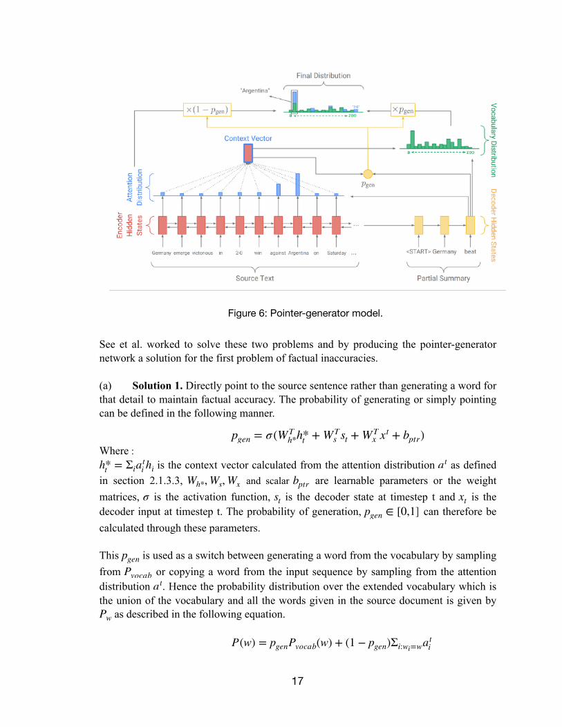
See et al. worked to solve these two problems and by producing the pointer-generator network a solution for the first problem of factual inaccuracies.

(a) Solution 1. Directly point to the source sentence rather than generating a word for that detail to maintain factual accuracy. The probability of generating or simply pointing can be defined in the following manner.

�Where : " is the context vector calculated from the attention distribution " as defined in section 2.1.3.3, " and scalar " are learnable parameters or the weight matrices, " is the activation function, " is the decoder state at timestep t and " is the decoder input at timestep t. The probability of generation, " can therefore be calculated through these parameters.

This " is used as a switch between generating a word from the vocabulary by sampling from " or copying a word from the input sequence by sampling from the attention distribution " . Hence the probability distribution over the extended vocabulary which is the union of the vocabulary and all the words given in the source document is given by " as described in the following equation.

"

pg en = σ (WTh *h *t + WT

s st + WTx xt + bptr)

h *t = Σiati h i at

Wh *, Ws, Wx bptrσ st xt

pg en ∈ [0,1]

pg enPvocab

at

Pw

P(w) = pg enPvocab(w) + (1 − pg en)Σi:wi= wati

�17

Figure 6: Pointer-generator model.

(b) Solution 2. Maintain a coverage vector to remember the sequence of words which have already arrived once in the summary and to reduce the probability of their repeated occurrence. The coverage vector is the sum all the attention distributions, which signifies the degree of coverage that those words have received from the attention mechanism so far and is given by the following equation :

" Where: " is the coverage vector and " is the attention distribution over each sentence at a single timestep.

2.3.3 Implementation Details of Pointer Generator Network

The pointer-generator network was implemented on both the CNN/Daily Mail dataset as well as our own dataset. The code originally implemented in Tensorflow version 1.0 has been trained on our own dataset after the suitable representation and preprocessing of the dataset. The dataset was first tokenized using the Stanford CoreNLP toolkit and then processed into .bin vocab files and the data was carefully chunked to meet the requirements for the dataset. The results obtained after training the pointer-generator network for 48hr on Nvidia TX2 server have been described as follows:

ct = Σt−1t′�= 0at′�

ct at

�18

Figure 7 : Decoded and reference summaries from the pointer-generator network.

�19

Figure 8 : Attention visualization on CNN/Daily Mail dataset.

Figure 9 : Attention visualization on our Dataset.

3. Speech Recognition Speech recognition is the process of giving machines the power to understand natural language, process it and then comprehend it to present the result in the form of a text. This field is an interdisciplinary field which is a subfield of computational linguistics that develops techniques to allow machines to process and translate speech into text.

The task of multimodal summarization takes audio as one of the inputs from the dataset and it is therefore extremely necessary to process the audio in a form such that is is able to be matched with the synchronous text and and the correspond video keyframes. It is therefore necessary to extract the features from audio and then apply our recognition model to process it further more to achieve the required results.

3.1 History

3.1.1 Early Approaches

The work on speech recognition has been going on since half a century now with Bell Labs researchers, Stephen Balashek, R. Biddulph, and K. H. Davis building “Audrey” for single-speaker digit recognition in 1952 [18]. Though there was a lot of research on speech recognition and language understating in the following years but the major breakthrough came in the 1980s which saw the introduction of the n-gram language models. In the following years with the advancement in computing power, the speech recognition technology became more and more accurate.

3.1.2 Mel-Frequency Cepstral Coefficients

The mel-frequency cepstrum (MFC) is a representation of short-term power spectrum of sound and are very similar to the principle components of the log spectra. They are based on a linear cosine transform of a log power spectrum on a non linear mel scale of frequency.

The mel-frequency cesptral coefficients (MFCC) are the coefficients that together make up the MFC. They are derived from a non-linear or cepstral representation of an audio clip. The MFCCs are more commonly viewed as features for speech recognition systems. The MFCCs imitate the natural features that a human recognizes while listening to sound. They are therefore inspired from human auditory track.

�20

3.2 Hidden Markov Models The hidden Markov models are statistical models that take into account sequential input and output a sequence of symbols or quantities. They are widely used in speech recognition systems because speech can be visualized as a Markov model for many stochastic purposes.

The HMMs are also extremely popular because they can be trained automatically and are simple and computationally feasible to use. The output for the HMMs is obtained by taking into account the output of various previous timesteps where the number of previous outputs that need to be taken is a parameter than can be tuned. The vector input to the HMMs consist of the MFCC features and the output is generated by taking a probability distribution over each phoneme in the output.

3.3 End-to-End Speech Recognition Since 2014, end-to-end speech recognition models have become the stalwarts in speech recognition technology. They are the current state of the art approach to solve the given problem statement. They are extremely powerful because they jointly learn all the components of a speech recognizer. As a result we do need to specify to the model any specific features that we think to be important to produce results. The model on the other hand self-learns the features it deems to be important through the provided data.

One of the major breakthroughs came with the “Listen, Attend and Spell” model [19] which applied the attention model used by Bahdanau et al. [14] for neural machine translation. The model has been described as follows :

3.3.1 Task Definition

Let " be the input sequence of filter bank spectra features (MFCCs) and " be the output sequence, a probability distribution over the output vocabulary. The task of the model is defined as the generation of probability of output " using the the outputs of the previous timesteps " and the input signal " for that timestep. It is formally defined as :

"

3.3.2 Listen, Attend and Spell

This model was described in 2016 by Chan et al. [19] and is one of the state of the art models for end-to-end speech recognition task. It identifies the features for input audio signal on its own and selectively pays attention to those features using attention model.

x = (x1, x2, …, xT )x = (y1, y2, …, yS)

yiy< i xi

P(y |x) = ΠiP(yi |x, y< i)

�21

The LAS model is based on the Encoder-Decoder architecture with attention. The Listener acts as the Encoder which is a pyramidal BiLSTM encoding of the input sequence x into higher dimensional features h, the speller is an attention-based decoder which generates the y characters from h. The result is obtained by producing a probability distribution over the output vocabulary and the experimental analysis of the LAS model has proven that it outperformed the state of the art models existing at that time including the HMM model for speech recognition.

As a result, model for multimodal summarization has been inspired from the LAS model and uses similar encoder structure to generate sequential encoding of input features.

�22

Figure 10 : Listen, Attend and Spell (LAS) model.

4. Video Recognition The third and the final task in order to achieve multimodal summarization the task of image recognition. This involves understanding the contents of an image and then relating them to the natural language. One of the most challenging tasks of computer vision is to recognize the images and perform tasks such as event detection, scene reconstruction, 3D pose restoration, image captioning and visual question answering. This is being extensively used today for self-driving cars and other autonomous vehicles like autonomous agricultural vehicles on Earth and autonomous Mars rovers.

The task of video recognition can be broken down into the task of identification of keyframe images and then applying the widely available image recognition algorithms to process and recognize the images. Therefore if we have a robust image recognition algorithm, we can extend it to video recognition as well.

4.1 History

4.1.1 Early Approaches

The task of video recognition as explained previously can be broken down to the task of image recognition which can further be broken down to solve the problem of pattern recognition. Images can be considered as patterns and can therefore be included in the main task of pattern recognition. The main task is to identify the particular patterns in images. The field of pattern recognition has been evolving for quite few decades with many sequence labeling algorithms as well as machine learning algorithms being applied for the same.

4.1.2 Machine Learning Approaches

The task of image recognition and classification has received major breakthrough with the application of various classification tasks being applied for images. The task of image classification can be solved through the state of the art machine learning models which allows more accurate results on the given dataset. One of the most popular classification techniques which have been applied for image classification are support vector machines.

Support Vector Machines (SVMs) are among the best supervised learning algorithms. They take into exhaustive consideration of vector representation of the training examples and divide the linearly separable labels with the help of margin and the greater the margin, the more accurate prediction there can be. Though they are defined for linearly separable classifiers, they are extended to non-linearly separable classifiers with the help of Kernels, which make the SVMs work like a charm for non-linearly separable data.

�23

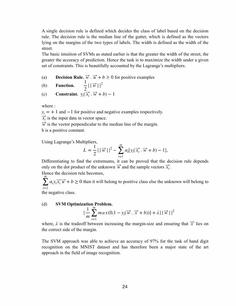
A single decision rule is defined which decides the class of label based on the decision rule. The decision rule is the median line of the gutter, which is defined as the vectors lying on the margins of the two types of labels. The width is defined as the width of the street. The basic intuition of SVMs as stated earlier is that the greater the width of the street, the greater the accuracy of prediction. Hence the task is to maximize the width under a given set of constraints. This is beautifully accounted by the Lagrange’s multipliers.

(a) Decision Rule. " for positive examples

(b) Function. "

(c) Constraint. "

where : " and " for positive and negative examples respectively. " is the input data in vector space. " is the vector perpendicular to the median line of the margin. b is a positive constant.

Using Lagrange’s Multipliers,

" ,

Differentiating to find the extremums, it can be proved that the decision rule depends only on the dot product of the unknown " and the sample vectors " . Hence the decision rule becomes,

" then it will belong to positive class else the unknown will belong to

the negative class.

(d) SVM Optimization Problem.

"

where, " is the tradeoff between increasing the margin-size and ensuring that " lies on the correct side of the margin.

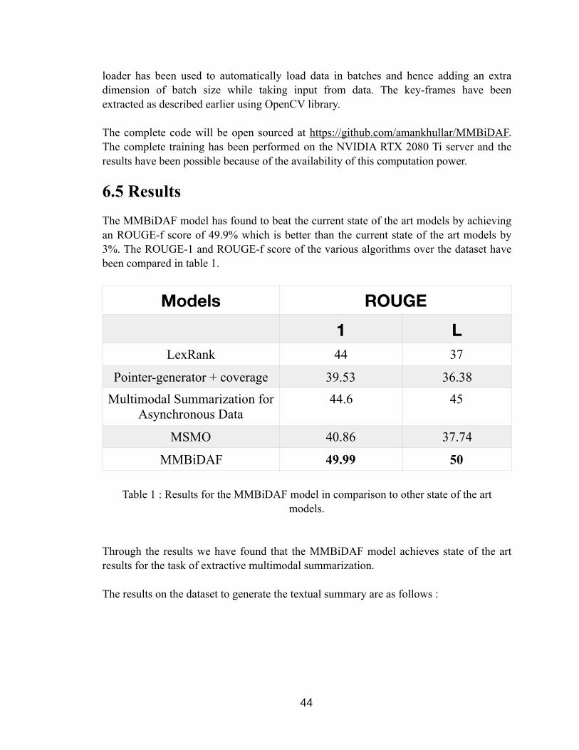
The SVM approach was able to achieve an accuracy of 97% for the task of hand digit recognition on the MNIST dataset and has therefore been a major state of the art approach in the field of image recognition.

w . u + b ≥ 012 | | w | |2

yi( xi . w + b) − 1

yi = + 1 −1xi w

L = 12 | | w | |2 −

m

∑i= 1

αi[yi( xi . w + b) − 1]

u xi

m

∑i= 1

αiyi xi u + b ≥ 0

[ 1m

m

∑i= 1

ma x(0,1 − yi( w . x + b))] + λ | | w | |2

λ x

�24

4.2 Convolutional Neural Networks ConvNets are deep, feedforward neural networks which are much easier to train and can be generalized much better than fully connected adjacent layers. They are widely used by the computer vision community to identify the various features in an image.

The ConvNets are designed to process data that comes in the form of multiple arrays. The architecture of ConvNets is a sequence of convolutional layers interspersed with activation functions and includes other layer including pooling layer, max-pooling layer and fully connected layer.

The convolutional layer essentially convolves (slides) over all the spatial locations in an image to carefully scrutinize the local features of images. A filter of appropriate size is selected and is maneuvered through the image with a specific stride.

The Pooling layer is responsible for making the image representation smaller and more manageable. It operates over each activation map independently. The pooling layer only reduces the spatial dimensions of the image and does not affect the depth of the image. Downsampling is an intermediate step involved to achieve pooling.

The maxpooling layer is used to achieve pooling. We take a filter of a fixed size and slide it over the entire image to take the max value of neuron in each filter area. The strides are designed to avoid overlap. Typically zero padding is not used. Finally the fully connected layer contains the entire network connecting input to produce the required output.

�25

Figure 11 : A typical CNN architecture. The outputs from each layer of a typical convolutional neural network applied to Samoyed dog where each rectangular image is a feature map.

4.3 Show, Attend and Tell Inspired by the work in machine translation and object detection, Xu et al. [20] introduced an attention based model that automatically learnt describe the contents of the image. Through the task of image captioning, Xu et al. ventured into the task of scene understating.

In order to understand the images, they also generated an encoder-decoder model with attention on particular parts of the images. The model essentially encoded the image using a convolutional neural network to extract the features and then applied an RNN layer over these extracted features by using an attention based decoder which selectively paid attention to important parts of the images to produce the output summary. The process has been shown in Figure 12. The decoder of the model is composed of LSTM cells which generate one word at every timestep conditioned on a context vector, the previous hidden state and the previously generated word.

5. Baseline Multimodal Summarization The task of multimodal summarization as described previously encompasses the tasks previously described of text summarization, speech recognition and video recognition. The increase in the volume of multimedia-data has made it difficult for the users to extract meaningful content from the vast amount of data. This is where the task of multimodal summarization comes into picture. It is able to collect the multitude of multimedia data and then present a succinct summary out of it which shall allow the users to understand the context of the data with much ease and give a relatively better perspective of the data.

�26

Figure 12 : The Show, Attend and Tell image captioning model.

5.1 History

5.1.1 Early Approaches

The task of MMS has been applied in the fields of meeting record summarization, sport video summarization, movie summarization and social media summarization. These all tasks have the availability of multimedia data and therefore it is a reasonable assumption that the benefit of application of the various MMS techniques in these areas will have the maximum impact. Meeting record summarization has been performed by Erol et al. [21], Gross et al. [22], sports video summarization has been performed by Tjondronegoro et al. [23], movie summarization has been performed by Mademlis et al. [24] and social media summarization has been performed by Shah et al. [25]. Though a lot of work has been performed in this field, the work that has been performed does not necessarily take into account all the modalities of data as well as do not apply the state of the art deep learning approaches. Moreover, the task that they deal with are the tasks of synchronous data summarization however one of the baseline models that is explained in the models secant involves the multimodal summarization of the asynchronous data.

5.2 Task Definition

5.2.1 Problem Formulation

The input is a collection of Multimodal data " related to a dataset were the each document " may or may not consist of an image along with the text in the document. " denotes the video and " denotes the cardinality of the set. The objective of multimodal summarization is to automatically generate textual sugary to represent the principle content of " .

5.2.2 Evaluation Metric

Since the multimodal summarization model produces a textual summary of the multimedia data, the same evaluation metrics namely, precision, recall and F1 scores can be used and most importantly the ROUGE scores can be used for the evaluation of the generated textual summary. This is able to measure the summary quality by matching the n-grams between the generated summary and the reference summary in the ROUGE-N evaluation metric.

Apart from the ROUGE scores which are essential for the evaluation of the generated textual summaries with respect to the reference summaries, researchers in the multimodal community have also introduced various metrics to evaluate the multimodal summaries. These summaries take into account the influence factor through the other media of data. These evaluation metric have been defined as follows :

. = {D1, …, D|D|}, {V1, …, V|V|}D = {Ti, Ii}

Vi | ∘ |

.

�27

(a) Content F1. Libovicky et al. [26] introduced the Content F1 evaluation metric which recognized the fact that the task of summarization was being carried out over the HOW2 dataset and there were certain words which occurred at the start of almost all the videos. These words were also present in the reference summary hence they increase the ROUGE score even when the model does not completely understand the data. This was prevented by post processing the data to remove these frequently occurring words from the dataset and then calculate the F1 score. This metric was then named as Content F1.

(b) Multimodal Automatic Evaluation (MMAE). This metric is used for the models which produce pictorial summary along with textual summary. Hence this becomes self in models having multimodal output for multimodal input data. The was introduced by Zhu et al. [27] and considered three aspects: salience of text, salience of image and relevance between text and image.

5.3 Dataset and Models

5.3.1 MSMO Dataset

Zhu et al. [27] collected a multimodal dataset similar to Hermann at al. [28]. They collected their large-scale multimodal dataset from Daily Mail website and annotated the pictorial summaries.

5.3.2 How2 Dataset

How2 is a large scale dataset for multimodal language understating [29]. The How2 dataset contains 79,114 instructional videos with English subtitles. The corpus can be recreated using the scripts and the metadata available at https://github.com/srvk/how2-dataset. The dataset has been collected from the YouTube instructional videos and the descriptions and the subtitles are taken as ground truth made available by the video creators.

�28

Figure 13 : How2 dataset with utterance-level English subtitle with Portuguese translation and the reference summary available in the form of abstract.

5.3.3 Extractive Asynchronous Multimodal Summarization

Li et al. [30] proposed a modern technique for extractive multimodal summarization for asynchronous collection of text, image, video and audio. The baseline experiments had been performed on their custom dataset which included asynchronous data. However, their work was extended in this project and evaluated on the synchronous dataset. In their paper, they proposed an approach to a generate textual summary from a set of asynchronous documents, images, audios and videos on the same topic. Since multimedia data are heterogeneous and contain more complex information than pure text does, MMS faces a great challenge in addressing the semantic gap between different modalities. The framework of their method is shown in Figure 14. For the audio information contained in videos, speech transcriptions is obtained through Automatic Speech Recognition (ASR) and designed a method to use these transcriptions selectively. For visual information, including the key-frames extracted from videos and the images that appear in documents, the joint representations of texts and images is learnt by using a neural network; then the text that is relevant to the image is identified. In this way, audio and visual information can be integrated into a textual summary. The model proposed by Li et al. has the following features :

(a) Readability Guidance Strategies. The basic premise of this strategy is that if there is a sentence in the document which is related to the audio, then the text in the document would be preferred rather than the sentence obtained after the automatic speech recognition. The similarity is obtained with the help of cosine similarity and a threshold is used to determine is the sentences are appropriately similar.

(b) Audio Guidance Strategies. For each adjacent speech transcription pairs, if audio score is smaller than a certain threshold value then the speech transcription should recommend the document text and the document text should not recommend speech transcription.

(c) Text-Image Matching. The main idea of text image matching is that semantic analysis is performed between text and image to learn the joint representation for textual

�29

Figure 14 : The framework for Asynchronous MMS Model

and visual modalities by using a model trained on Flickr 30K dataset. The framework model by Wang et al. [31] is used to achieve the state of the art performance for text-image matching task on the Flickr 30K dataset.

(d) Budgeted optimization of submodular functions.

Where : T is the set of sentences, S is the summary, " is the length (number of words) of sentence s, L is the maximum length of the summary and F(S) is the summary score.

(e) Salience of text.

Where : " is the damping factor that is usually set at 0.85, N is the total number of text units, " is the relationship between the text unit " and " which is computed as follows :

" The text unit " is represented by averaging the embeddings in " and " denotes the similarity between the two texts.

(f) Objective function. The objective function considers all the modalities and is mathematically defines as follows :

Where: " is the summary score obtained by text salience, " is the summary score obtained by image salience. This is a monotone submodular function and a greedy algorithm can be applied to obtain the optimum value for this function and the argument sentences for this value is generated multimodal summary.

5.3.3.1 Implementation Details

The entire algorithm has been implemented on our own dataset to evaluate the accuracy of the generated summary on the self generated dataset. The OpenCV framework has been used to extract salient key-frames from the videos and the these key-frames are then matched with the speech transcriptions and the document text. The similarity matrix has been produced by incorporating specific changes in the code for the LexRank algorithm. The submodular function has been optimized using the greedy algorithm described by Lin et al. [32]. The for the implementation of the paper on the our own dataset are as follows:

ls

μ Mjiti tjMji = sim(tj, ti)

ti ti sim( ∘ )

Ms Mc

�30

m a xs⊆T{F(S) : ∑s∈S

ls ≤ L}

Sa(ti) = μΣjSa(tj) . Mji + 1 − μN

Fm(S) = 1Ms

Σti∈SSa(ti) + 1Mc

Σpi∈SIm(pi)bi − λm

|S|Σti,tj∈Ssim(ti, tj)

�31

Figure 15 : List of generated summaries.

Figure 16 : Source transcript in the dataset

�32

Figure 17 : Generated summary from the source data.

Figure 18 : ROUGE score evaluation of the generated summary.

5.3.4 Multimodal Summarization with Multimodal Output

Multimodal Summarization with Multimodal Output (MSMO) [27] is a novel multimodal summarization task, which takes the news from the defined dataset with images as input, and finally outputs a pictorial summary. They constructed a large scale corpus for MSMO study. They proposed an abstractive multimodal summarization model to jointly generate summary and the most relevant image. They proposed a multimodal automatic evaluation (MMAE) method which has been described in section 5.3.1. The text encoder and the summary decoder have been inspired from the Pointer-Generator networks.

Multimodal attention layer has been placed on top of the textual and visual attention layer. This layer acts as a distribution between the text visual features of the data hence this layer is built on top of the previous attention layer which specifies the attention required to be given to specific words and images. The second level of attention layer is required to weigh the importance that needs to be give to the visual and textual features all together. Hence this hierarchal attention model is able to generate an output multimodal summary which performs well on their dataset and they were able to prove good results using the MMAE metric. The architect of the MSMO model has been described in figure 19. The model can further be described using the mathematical equations built on top of the pointer-generator model as described in section 2.3.2 as :

�33

Figure 19 : Architecture for the MSMO model

ettxt = vT

txt(Wtxtcttxt + Utxtst)

etimg = vT

img (Wimg ctimg + Uimg st)

α ttxt = sof t m a x (et

txt)αt

img = sof t m a x (etimg )

ctmm = α t

txtcttxt + αt

img ctimg

Where: " is the attention weight for the text context vector and " is the attention weight for the image context vector. These two distributions are combined with the context vectors of the text and the image respectively to produce the combined multimodal context vector. This is passed to the decoder which then generates a probability distribution over the output vocabulary and output images to select the most accurate word and image at each timestep and in turn produce a good multimodal output summary.

5.3.4.1 Implementation Details

The MSMO model has been built on top of the pointer-generator network and hence most of the code has been reused from the pointer generator network and this too has been coded using the Tensorflow framework in version 1.0. The authors were kind enough to share the code with me for my research purpose and I implemented the code on our dataset to get the ROUGE score results for the same. The training step of the code in NVIDIA TX2 has been shown in figure 20.

α ttxt αt

img

�34

Figure 20 : Training of the MSMO model on our dataset.

�35

Chapter II MultiModal BiDirectional

Attention Flow (MMBiDAF)

�36

Figure 21 : Architecture for MMBiDAF model.

6. MultiModal BiDirectional Attention Flow

The MMBiDAF model (figure 21) is the proposed model for carrying out the defined task of multimodal summarization which has been inspired from the various previous state of the art models existing in the literature. This model was chosen since it encompasses all the input modalities, calculates the similarity between them and then uses a multimodal attention later on top of image-aware and audio-aware texts to get an output distribution over the source document.

The model is used for extractive summarization in which at each timestep the most probable sentences are selected and chosen as part of the output summary. The summary terminates when the probability of a special <End Of Summary> token is the greatest. The proposed model is inherently a combination of Bidirectional Attention Flow [33] and Multimodal Attention models [34]. Our model follows the high-level structure of embedding layer, encoder layer, bidirectional attention layer, modality aware sequence modeling layer, multimodal attention layer and finally an output layer. The model is explained in complete detail in the following sections.

6.1 Model Explanation

6.1.1 Text Embedding Layer

Let the input document be described as " where " is the embedded sentence obtained by averaging the pertained GloVE embeddings of the words included in the sentence. ’T’ is the number of sentences in the source document. Hence each sentence is now described as a vector with dimension equal to the embedding dimension (D). Hence " .

In order to further refine the generated embeddings, the embedded sentences are undergone through the following steps :

• Each Embedding is projected to have the dimensionality H. By making " a learnable parameter, each embedding vector " is mapped to " .

• A Highway Network [35] is applied to refine the embedded representation. Given an input vector " , one-layer highway network computes

" " " Where: " and " are learnable parameters. The hidden vectors are therefore transformed using this Highway Network and this transformation.

(X1, X2, …, XT ) Xi

Xi ∈ ℝD ∀i

Wproj ∈ ℝH×D

Xi h i = Wproj Xi ∈ ℝH

h ig = σ (Wg h i + bg ) ∈ ℝH

t = ReLU(Wth i + bt) ∈ ℝH

h ′�i = g ⊙ t + (1 − g ) ⊙ h i ∈ ℝH

Wg , Wt ∈ ℝH×H bg , bt ∈ ℝH

�37

6.1.2 Audio Embedding Layer

The audio embedding layer is basically the feature extraction layer input audio signals. The MFCC features of the input audio signals are extracted to generate audio envelopes of embedded dimension. The input audio signal is therefore obtained on parts where each part signifies a frequency envelop which have been extracted using the MFCC algorithm. The audio signal is therefore obtained in form of " where A is the number of envelopes and each " where " is the embedding dimension for the generated discrete audio signals.

In order to further refine the audio embeddings, the audio embeddings are passed through the same two steps of projection and Highway Network to refine the generated audio embeddings. After passing the audio embeddings through these steps, we obtain the embedded audios in the dimension equal to the dimension of the hidden state. Hence we now get the audio embeddings as " .

6.1.3 Image Embedding Layer

The third and the last input modality is the video in the dataset. The videos are first preprocessed to extract the key-frames from the video. The extraction of salient frames is an ongoing are of research and we have used a naive OpenCV key-frame extraction algorithm based on the change in the histograms of the adjacent frames.

The obtained images may be of different sizes and they are therefor first normalized and to obtain images of equal dimension. Hence the video is now available in the form of key-frame images where each image is of the form given by " where " where " is the normalized image size.

The obtained images are then embedded using the ResNet [36] network which extracts the features from the input images to make them of suitable dimension. A linear layer is then passed through the obtained embedded images to represent every image with fixed size dimension.

In order to further refine the image embeddings, the image embeddings like the audio and the text embeddings are passed through the same two steps of projection and Highway Network to refine the generated image embeddings. After passing the image embeddings through these steps, we obtain the embedded images in the dimension equal to the dimension of the hidden state. Hence we now get the image embeddings as " .

(Y1, Y2, …, YA)Yi ∈ ℝD1 D1

Yi ∈ ℝH ∀i

(Z1, Z2, …, ZI)Zi ∈ ℝd2×d2 ∀i d2

Zi ∈ ℝH ∀i

�38

6.1.4 Encoder Layer

The generated text, audio and image embeddings are fed into the encoder layer which is composed of a Bidirectional LSTM network. This layer is responsible for incorporating temporal dependencies between the generated embeddings. The embeddings are therefore transformed into sequential encodings for all the three types of modalities of data. The encoded output is the LSTM’s hidden state at each timestep :

" " "

The output from the Encoder layer is therefore of dimension 2H which is twice the hidden size of the network.

6.1.5 Attention Flow Layer

The attention flow layer is responsible for generating image-aware textual vectors and audio-aware textual vectors. This intuitively signifies that the text is now aware of the correspond audio and image dataset after it passes through this layer.

These are computed using the similarity matrix which is a trainable matrix between the separate modalities. The similarity between each textual sentence and all the audio vectors as well as the similarity between each textual sentence and every image is calculated.

This similarity matrix is then used to calculate attention weights each textual sentence shall give to the different modality.

The 2H dimensional images and text shall be passed through the similarity matrix whose dimension shall be " where T is the number of text sentences and I is the number of key-frame images. The similarity matrix shall be computed as :

"

where " represents the column vector of the H matrix which is the sentence embedding matrix and similarly " represents the column vector of U matrix which is the embedding matrix for each image. Hence " and " .

Similarly the encoded text and audio are then passed through the another similarity matrix which calculates the similarity between the encoded text and the encoded audio.

h ′�i, f wd = LSTM(h ′�i−1, h i) ∈ ℝH

h ′�i,rev = LSTM(h ′�i+ 1, h i) ∈ ℝH

h ′�i = [h ′�i, f wd; h ′�i,rev] ∈ ℝ2H

S ∈ ℝT×I

S = α(H:t, U:i) ∈ ℝ

H:tU:i

H ∈ ℝ2H×T U ∈ ℝ2H×I

�39

The trainable similarity function needs to be calculated and is defined as " . These values are calculated each pair (h, u) in the similarity matrix where "

6.1.5.1 Text-to-Image Attention

The attention weights over all the key-frame images in the given dataset can then be calculated as " . The text-to-image attention signifies which images are most relevant to each sentence. Hence " is a probability distribution over the complete set of images.

Now the attended image vectors for the entire text will be " which signifies that for every sentence the attention given to each image has been incorporated. Hence the text that we now have is attentive to the images and knows which image it needs to pay attention to. This is calculated using the following equation :

" Where: " are the text vectors which are aware of the corresponding image.

6.1.5.2 Image-to-Text Attention

This signifies which of the sentences has the closest similarity to each keyframe image. For every image, the similarity score over all the sentences is calculated to understand which of the sentences are the closest to the given keyframe.

The attention weights are obtained using " which tells the probability distribution of all the sentences over the given image.

The context vector for the images can then be calculated using :

"

This indicates the image to text attention output. For each sentence, " , we obtain the output " of the Bidirectional Attention Flow layer by combing text hidden state " , the Text-to-Image attention output " , the image-to-text attention " :

"

where " is the element wise multiplication.

α(h , u ) = wTsim[h ; u ; h ⊙ u ]

wsim ∈ ℝ6H

at = sof t ma x(St:) ∈ ℝI

at

U ∈ ℝ2H×T

U:t = ΣjatjU:j ∈ ℝ2H

U ∈ ℝ2H×T

bt = sof t ma x(ma xcolS) ∈ ℝT

h = ΣtbtH:t ∈ ℝ2H

i ∈ 1,…, Tg i

Xi U:i h

g i = [Xi; Ui; Xi ⊙ Ui; h ] ∈ ℝ8H ∀i ∈ {1,…, T}

⊙

�40

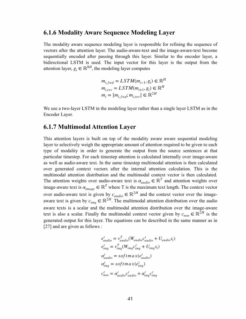
6.1.6 Modality Aware Sequence Modeling Layer

The modality aware sequence modeling layer is responsible for refining the sequence of vectors after the attention layer. The audio-aware-text and the image-aware-text become sequentially encoded after passing through this layer. Similar to the encoder layer, a bidirectional LSTM is used. The input vector for this layer is the output from the attention layer, " , the modeling layer computes

" " "

We use a two-layer LSTM in the modeling layer rather than a single layer LSTM as in the Encoder Layer.

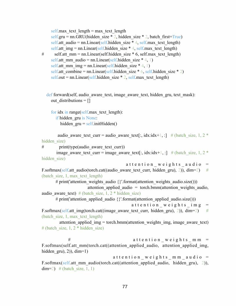
6.1.7 Multimodal Attention Layer

This attention layers is built on top of the modality aware aware sequential modeling layer to selectively weigh the appropriate amount of attention required to be given to each type of modality in order to generate the output from the source sentences at that particular timestep. For each timestep attention is calculated internally over image-aware as well as audio-aware text. In the same timestep multimodal attention is then calculated over generated context vectors after the internal attention calculation. This is the multimodal attention distribution and the multimodal context vector is then calculated. The attention weights over audio-aware text is " and attention weights over image-aware text is " where T is the maximum text length. The context vector over audio-aware text is given by " and the context vector over the image-aware text is given by " . The multimodal attention distribution over the audio aware texts is a scalar and the multimodal attention distribution over the image-aware text is also a scalar. Finally the multimodal context vector given by " is the generated output for this layer. The equations can be described in the same manner as in [27] and are given as follows :

g i ∈ ℝ8H

mi, f wd = LSTM(mi−1, g i) ∈ ℝH

mi,rev = LSTM(mi+ 1, g i) ∈ ℝH

mi = [mi, f wd; mi,rev] ∈ ℝ2H

αau dio ∈ ℝT

αimag e ∈ ℝT

cau dio ∈ ℝ2H

cimg ∈ ℝ2H

cmm ∈ ℝ2H

�41

etau dio = vT

au dio(Wau dioctau dio+ Uau diost)

etimg = vT

img (Wimg ctimg + Uimg st)

αtau dio = sof t m a x (et

au dio)αt

img = sof t m a x (etimg )

ctmm = αt

au dioctau dio+ αt

img ctimg

6.1.8 Output Layer

The output layer takes as input the multimodal context vector produced by the Multimodal Attention layer, " . This is then fed into a GRU cell which acts as a sequential layer before generating the final output to give a sequential encoding over the final output distribution. A softmax function is then applied over a fully connected linear layer over the output distribution. This gives us the probability of selecting each sentence at each timestep and the sentence with the maximum probability is chosen at that timestep. This can be quantified as follows :

" " " " Where: " is the output vector at timestep t, " are respectively the audio aware text and the image aware text at timestep t. " is the multimodal context vector at timestep t. At every timestep the GRU cell receives the previous hidden state and the current output from the previous layers as its input and then it converts it into a temporal encoding which is important for sequence dependent output like the textual summary. It is also necessary to take linear transform using the trainable weight matrices " and " where T is the maximum length of the input text vectors.

Finally the softmax layer produces an output distribution over the source sentences in the document and at each timestep a probability distribution over the source sentences is calculated and the sentence with the maximum probability at a given timestep is selected to be a part of the output summar and trained using negative log probability of the target. The output summary is therefore generated from the given input multimodal data.

6.2 Multimodal Dataset Resources of the corpus were driven from online courses provided by Coursera using coursera-dl, a python script to download course materials available on Coursera. Every lecture is accompanied by following resources : Videos (mp4), transcripts (txt), timed transcripts (srt), lecture notes (pdf, ppt). Out of 3000 courses, 25 courses were selected with a total of 965 videos and corresponding transcripts. Each directory contains 5 folders with each directory representing a course. The course contains several video lectures and the corresponding transcripts. The Audios have been extracted from the videos using the ffmpeg scripts. The audio-features are the Mel-frequency cepstral coefficients (MFCC) features which take human perception sensitivity with respect to frequency into consideration. These have been extracted for speech feature recognition. The Srt folder

cmm

ot = [yt; zt; cmmt]ot = Wootot, h t = GRU(ot, h t−1)ot = sof t ma x(Wf ot)

ot yt, ztcmmt

Wo ∈ ℝ6H×2H

Wf ∈ ℝ2H×T

�42

contains the timed transcripts of each video and used for specific transcript for video frames. The directory structure of the dataset is shown in figure 22.

6.3 Evaluation Metric Since the task that we are pursuing involves the generation of multimodal summary in a textual form, it is convenient to use the widely accepted ROUGE scores for determining the accuracy of the generated output summary with respect to the self annotated reference summary. Hence for this task, we have used the ROUGE as described in section 2.2.2.

6.4 Implementation Details The complete model has been implemented using PyTorch machine learning framework in python 3.0 programming language. The Rouge library has been used to evaluate the Rouge scores. The pre-trained GloVE vectors have been used and the text embedding size is 300 features while the audio embedding size is 128 features and the image embedding size is of 2048 features. The hidden size is taken to be 100 while dropout is applied to counter the problem of overfitting and the dropout probability is taken to be 0.2. The maximum text length has been identified from the dataset and has been found out to be of size 405. The number of epochs have been set to 100. Seaborn library has been used to obtain the heat map to visualize the multimodal attention distribution. NLTK library has been used for sentence and word tokenization.

The complete dataset has been preprocessed to remove the stopwords and the extra words in the course transcripts for instance the occurrence of the word ‘[MUSIC]’ in the source transcript has been removed while preprocessing the data. The gensim library has been used to extract the pertained GloVE vectors for the source words and the average of these embedded words is calculated to produce a sentence embedding. The PyTorch Data

�43

Dataset

1

Transcripts Videos Audio Audio-

Features

Srt

24

Transcripts Srt

………………………

…

Figure 22 : Directory structure of the multimodal dataset

loader has been used to automatically load data in batches and hence adding an extra dimension of batch size while taking input from data. The key-frames have been extracted as described earlier using OpenCV library.

The complete code will be open sourced at https://github.com/amankhullar/MMBiDAF. The complete training has been performed on the NVIDIA RTX 2080 Ti server and the results have been possible because of the availability of this computation power.

6.5 Results The MMBiDAF model has found to beat the current state of the art models by achieving an ROUGE-f score of 49.9% which is better than the current state of the art models by 3%. The ROUGE-1 and ROUGE-f score of the various algorithms over the dataset have been compared in table 1.

Through the results we have found that the MMBiDAF model achieves state of the art results for the task of extractive multimodal summarization.

The results on the dataset to generate the textual summary are as follows :

Models ROUGE1 L

LexRank 44 37

Pointer-generator + coverage 39.53 36.38

Multimodal Summarization for Asynchronous Data

44.6 45

MSMO 40.86 37.74

MMBiDAF 49.99 50

�44

Table 1 : Results for the MMBiDAF model in comparison to other state of the art models.

�45

Figure 23 : Source transcript.

Figure 24 : One of the key frames extracted from the video.

�46

Figure 25 : Generated summaries of the first four videos.

Figure 26 : Attention visualization for first video.

�47

Figure 27 and 28 : Attention distribution over the various sentences in the course videos.

The results have been obtained by using the Negative Log Likelihood. The loss is therefore given by

" Where : " is the reference target sentence. This is inspired from the choice of the pointer-generator function and has proven to obtain good results.

Backpropagation algorithm is then applied to train the learnable parameters and get the result.

losst = − log P(si*)

(si*)

�48

�49

Chapter III Conclusion and Beyond

7. Conclusion This thesis tackles the problem of multimodal summarization which is defined as the task of generating output summary taking into account the different multimedia data as input. The output summary may be presented in single modality or multiple modalities and this work presents the output in the form of textual modality.

In the thesis, the foundations of natural language processing in general and multimodal summarization in specific have been explored. Since the field of Multimodal Summarization encompasses the textual, audio and visual dataset, the foundations of these modalities have been explored and further built upon. The breakthrough models in the field of deep learning namely listen, attend and tell and show, attend and tell have also been described through which our model has been inspired. The explanation of these models has been listed in order to give the user a better understanding of the existing state of the art deep learning approaches. The baseline models have been implemented on our own dataset and the widely available dataset to explore the existent state of the art techniques. The datasets have been carefully preprocessed and chunked to suit the baseline model specifications.

The last part of this thesis presents the novel work of this thesis, the MultiModal Bidirectional Attention Flow Model (MMBiDAF). The architecture of the model has been carefully built to integrate all the modalities and draw similarity between them to carefully generate the text which is attentive of both image and audio which further receives an attention layer to select from the audio-aware or the image-aware text. The model is then able to generate a summary by extracting the most important sentences from the given source text. The results of the model have shown to outperform the existing state of the art models in the literature. MMBiDAF is compared with Lex Rank, pointer generator model, asynchronous summarization model and the MSMO model and it has been observed that MMBiDAF achieves a ROUGE-1 score of 49.9% and ROUGE-L score of 50.0%.

�50

8. Beyond Though MMBiDAF model beats the existing state of the art models in the field of extractive multimodal summarization, however there are a large number of areas where the proposed model can be modified and improved upon.

First of all, a new state of the art technique for NLP-training called Bidirectional Encoder Representation from Transformers (BERT) [37] can be applied which allows the model to be be built upon the existing pre-trained contextual representations. This gives NLP models the power to learn the context of the word occurring in the sentence. This is important for words like ‘bank’ which have completely different meaning when being used to describe river bank and when being used to describe the financial institution.

Secondly, the described work includes a vanilla approach for extracting the key-frame images however with the advancements in the techniques to extract the keyframe images from a given video.

Lastly, another interesting domain to build upon would be the same high-dimensional embedding space of the text, audio and video representation. The proposed work is able to perform well because the wearable weight matrix is able to learn the differences in the embedding space however other techniques for representing the modalities in a joint embedding space can be tried upon. This can be facilitated by including beam search at every timestep to extract a set of best sentences rather than a single sentence from the output distributions at each timestep.

�51

�52

9. References [1] Turing, A. M. (1950). "Computing Machinery and Intelligence" (PDF). Mind (59): 433.

[2] H. P. Luhn, “The automatic creation of literature abstracts,” IBM J. Res. Dev., vol. 2, no. 2, pp. 159–165, Apr.1958. [Online]. Available: http://dx.doi.org/10.1147/rd.22.0159

[3] A. Nenkova and K. McKeown, “Automatic summarization,” Foundations and Trends in Information Retrieval, vol. 5, pp. 103–233, 2011.

[4] J.S. Griggs “TL;DR Automatic Summarization With Textual Annotations”.

[5] LexRank: Graph-based Lexical Centrality as Salience in Text Summarization, vol. 22, 2004

[6] Page, Larry, "PageRank: Bringing Order to the Web". Archived from the original on May 6, 2002. Retrieved 2016-09-11., Stanford Digital Library Project, talk. August 18, 1997 (archived 2002)

[7] R. Mihalcea and P. Tarau, “TextRank: Bringing order into texts,” in Proceedings of EMNLP-04and the 2004 Conference on Empirical Methods in Natural Language Processing, July 2004.

[8] J. Kupiec, J. Pedersen, and F. Chen, “A trainable document summarizer,” in Proceedings of the 18th Annual International ACM SIGIR Conference on Research and Development in Information Retrieval, ser. SIGIR ’95. New York, NY, USA: ACM, 1995, pp. 68–73. [Online]. Available: http://doi.acm.org/10.1145/215206.215333

[9] J. M. Conroy and D. P. O’leary, “Text summarization via hidden markov models,” in Proceedings of the 24th Annual International ACM SIGIR Conference on Research and Development in Information Retrieval, ser. SIGIR ’01. New York, NY, USA: ACM, 2001, pp. 406–407. [Online]. Available: http://doi.acm.org/10.1145/383952.384042

[10] LeCun, Yann; Bengio, Yoshua; Hinton, Geoffrey (2015). "Deep learning". Nature. 521 (7553): 436–444. doi:10.1038/nature14539. PMID 26017442.

[11] Rumelhart, David E.; Hinton, Geoffrey E.; Williams, Ronald J. (8 October 1986). "Learning representations by back-propagating errors". Nature. 323 (6088): 533–536. Bibcode:1986Natur.323..533R. doi:10.1038/323533a0.

[12] Sepp Hochreiter; Jürgen Schmidhuber (1997). "Long short-term memory". Neural Computation. 9 (8): 1735–1780. doi:10.1162/neco.1997.9.8.1735. PMID 9377276.

�53

[13] Christpopher Olah. 2015. Understanding LSTM Networks. Colah’s blog.

[14] Dzmitry Bahdanau, Kyunghyun Cho, and Yoshua Bengio. 2015. Neural machine translation by jointly learning to align and translate. In International Conference on Learning Representations.

[15] A. Nenkova and K. McKeown, “Automatic summarization,” Foundations and Trends in Information Retrieval, vol. 5, pp. 103–233, 2011.

[16] R. Nallapati, B. Zhou, C. dos Santos, C¸ . glar Gulc¸ehre, and B. Xiang, “Abstractive text summarization using sequence-to-sequence RNNs and beyond,” CoNLL 2016, p. 280, 2016.

[17] Abigail See, Peter J. Liu, and Christopher D. Manning. 2017. Get to the point: Summarization with pointer generator networks. In Proceedings of the Annual Meeting of the Association for Computational Linguistics (ACL), pages 1073–1083.

[18] "IBM-Shoebox-front.jpg". androidauthority.net. Retrieved 4 April 2019.

[19] Chan, William; Jaitly, Navdeep; Le, Quoc; Vinyals, Oriol (2016). "Listen, Attend and Spell: A Neural Network for Large Vocabulary Conversational Speech Recognition". ICASSP.

[20] Xu, K. et al. Show, attend and tell: Neural image caption generation with visual attention. In Proc. International Conference on Learning Representations http://arxiv.org/abs/1502.03044 (2015).

[21] Berna Erol, D-S Lee, and Jonathan Hull. 2003. Multimodal summarization of meeting recordings. In Multimedia and Expo, 2003. ICME’03. Proceedings. 2003 International Conference on, volume 3, pages III–25. IEEE.

[22] Ralph Gross, Michael Bett, Hua Yu, Xiaojin Zhu, Yue Pan, Jie Yang, and Alex Waibel. 2000. Towards a multimodal meeting record. In Multimedia and Expo, 2000. ICME 2000. 2000 IEEE International Conference on, volume 3, pages 1593–1596. IEEE.

[23] Dian Tjondronegoro, Xiaohui Tao, Johannes Sasongko, and Cher Han Lau. 2011. Multi-modal summarization of key events and top players in sports tournament videos. In Applications of Computer Vision (WACV), 2011 IEEE Workshop on, pages 471–478. IEEE.

[24] Ioannis Mademlis, Anastasios Tefas, Nikos Nikolaidis, and Ioannis Pitas. 2016. Multimodal stereoscopic movie summarization conforming to narrative characteristics. IEEE Transactions on Image Processing, 25(12):5828–5840.

�54

[25] Rajiv Ratn Shah, Anwar Dilawar Shaikh, Yi Yu, Wenjing Geng, Roger Zimmermann, and Gangshan Wu. 2015. Eventbuilder: Real-time multimedia event summarization by visualizing social media. In Proceedings of the 23rd ACM international conference on Multimedia, pages 185–188. ACM.

[26] Jindˇrich Libovický, Shruti Palaskar, Spandana Gella, and Florian Metze. Multimodal abstractive summarization of open-domain videos. In Proceedings of the Workshop on Visually Grounded Interaction and Language (ViGIL). NIPS, 2018.

[27] Haoran Li, Junnan Zhu, Cong Ma, Jiajun Zhang, and Chengqing Zong. 2018. Multi-modal summarization with Multi-modal output. In Proceedings of the Conference on Empirical Methods in Natural Language Processing (EMNLP), pages 4154-4164.

[28] Karl Moritz Hermann, Tomas Kocisky, Edward Grefenstette, Lasse Espeholt,Will Kay, Mustafa Suleyman, and Phil Blunsom. 2015. Teaching machines to read and comprehend. In Proceedings of Neural Information Processing Systems (NIPS), pages 1693–1701.

[29] Ramon Sanabria, Ozan Caglayan, Shruti Palaskar, Desmond Elliott, Loïc Barrault, Lucia Specia, and Florian Metze. How2: a large-scale dataset for multimodal language understanding. In Proceedings of the Workshop on Visually Grounded Interaction and Language (ViGIL). NIPS, 2018.

[30] Haoran Li, Junnan Zhu, Cong Ma, Jiajun Zhang, and Chengqing Zong. 2017. Multi-modal summarization for asynchronous collection of text, image, audio and video. In Proceedings of the Conference on Empirical Methods in Natural Language Processing (EMNLP), pages 1092–1102.

[31] Liwei Wang, Yin Li, and Svetlana Lazebnik. 2016a. Learning deep structure preserving image-text embeddings. In Proceedings of the IEEE Conference on Computer Vision and Pattern Recognition, pages 5005–5013.

[32] Hui Lin and Jeff Bilmes. 2010. Multi-document summarization via budgeted maximization of submodular functions. In Human Language Technologies: The 2010 Annual Conference of the North American Chapter of the Association for Computational Linguistics, pages 912–920. Association for Computational Linguistics.

[33] Minjoon Seo, Aniruddha Kembhavi, Ali Farhadi, and Hannaneh Hajishirzi. Bidirectional attention flow for machine comprehension. arXiv preprint arXiv:1611.01603, 2016.

�55

[34] Haoran Li, Junnan Zhu, Tianshang Liu, Jiajun Zhang, and Chengqing Zong. 2018a. Multi-modal sentence summarization with modality attention and image filtering. In Proceedings of the Twenty-Fifth International Joint Conference on Artificial Intelligence (IJCAI), pages 4152–4158.

[35] Rupesh Kumar Srivastava, Klaus Greff, and Jürgen Schmidhuber. Highway networks. arXiv preprint arXiv:1505.00387, 2015.

[36] He, Kaiming; Zhang, Xiangyu; Ren, Shaoqing; Sun, Jian (2015-12-10). "Deep Residual Learning for Image Recognition". arXiv:1512.03385

[37] Jacob Devlin, Ming-Wei Chang, Kenton Lee, and Kristina Toutanova. 2018. BERT: Pre-training of Deep Bidirectional Transformers for Language Understanding. CoRR abs/1810.04805 (2018).

�56

Grammarly Report generated on Monday, May 27, 2019, 12:04 PM Page 1 of 25

29

7

6

5

12

6

2

1

32

9

2

3

1

45

27

26

12

11

5

DOCUMENT

Thesis_doc_2SCORE

60 ISSUES FOUND IN THIS TEXT

278PLAGIARISM

7%

Contextual Spelling 47Misspelled Words

Confused Words

Unknown Words

Mixed Dialects of English

Grammar 21Determiner Use (a/an/the/this, etc.)

Faulty Subject-Verb Agreement

Incorrect Verb Forms

Wrong or Missing Prepositions

Punctuation 43Punctuation in Compound/Complex Sentences

Comma Misuse within Clauses

Closing Punctuation

Sentence Structure 4Incomplete Sentences

Misplaced Words or Phrases

Style 126Passive Voice Misuse

Improper Formatting

Possible Dialectisms

Intricate Text

Wordy Sentences

Inappropriate Colloquialisms

of 100

Grammarly Report generated on Monday, May 27, 2019, 12:04 PM Page 2 of 25

37

Vocabulary enhancement 37Word Choice

Grammarly Report generated on Monday, May 27, 2019, 12:06 PM Page 1 of 43

54

12

9

6

1

56

12

6

6

5

1

1

1

83

15

6

3

1

124

DOCUMENT

Thesis_doc_1SCORE

56 ISSUES FOUND IN THIS TEXT

749PLAGIARISM

7%

Contextual Spelling 82Misspelled Words

Confused Words

Mixed Dialects of English

Unknown Words

Commonly Confused Words

Grammar 88Determiner Use (a/an/the/this, etc.)

Faulty Subject-Verb Agreement

Wrong or Missing Prepositions

Incorrect Verb Forms

Incorrect Noun Number

Conjunction Use

Pronoun Use

Misuse of Quantifiers

Punctuation 98Punctuation in Compound/Complex Sentences

Comma Misuse within Clauses

Sentence Structure 10Misplaced Words or Phrases

Incomplete Sentences

Faulty Parallelism

Style 317Passive Voice Misuse

of 100

Grammarly Report generated on Monday, May 27, 2019, 12:06 PM Page 2 of 43

73

65

34

19

2

154

Possible Dialectisms

Improper Formatting

Wordy Sentences

Intricate Text

Inappropriate Colloquialisms

Vocabulary enhancement 154Word Choice

10. Appendix A Code for models.py

import numpy as np import torch from layers.encoding import * from layers.attention import * import torch.nn as nn

class MMBiDAF(nn.Module): """ The combination of the Bidirectional Attention Flow model and the Multimodal Attention Layer model.

Follows a high-level structure inspired from the BiDAF implementation by Chris Chute.

- Embedding layer : Embed the text, audio and the video into suitable embeddings using Glove, MFCC and VGG respectively. - Encoder layer : Encode the embedded sequence. - Attention Flow layer : Apply the bidirectional attention mechanism for the multimodal data. - Modality aware encoding : Encode the modality aware sequence - Multimodal Attention : Apply the attention mechanism for the separate modality of data. - Ouput layer : Simple Softmax layer to generate the probability distribution over the textual data for extractive summary. Args: word_vectors (torch.Tensor) : Pre-trained word vectors (GLoVE). image_vectors (torch.Tensor) : Pre-trained image features (ResNet). audio_vectors (torch.Tensor) : Pre-trained audio features (MFCC). hidden_size (int) : Number of features in the hidden state at each layer. drop_prob (float) : Dropout probability. """

def __init__(self, hidden_size, text_embedding_size, audio_embedding_size, drop_prob=0., max_text_length=405): super(MMBiDAF, self).__init__() self.emb = Embedding(embedding_size=text_embedding_size, hidden_size=hidden_size, drop_prob=drop_prob)

�57

self.a_emb = Embedding(embedding_size=audio_embedding_size, # Since audio embedding size is not 300, we need another highway encoder layer hidden_size=hidden_size, # and we cannot increase the hidden size beyond 100 drop_prob=drop_prob)

self.text_enc = RNNEncoder(input_size=hidden_size, hidden_size=hidden_size, num_layers=1, drop_prob=drop_prob)

self.audio_enc = RNNEncoder(input_size=hidden_size, hidden_size=hidden_size, num_layers=1, drop_prob=drop_prob)

self.image_enc = RNNEncoder(input_size=hidden_size, hidden_size=hidden_size, num_layers=1, drop_prob=drop_prob)

self.image_keyframes_emb = ImageEmbedding(encoded_image_size=2)

self.bidaf_att_audio = BiDAFAttention(2*hidden_size, drop_prob=drop_prob)

self.bidaf_att_image = BiDAFAttention(2*hidden_size, drop_prob=drop_prob)

self.mod_t_a = RNNEncoder(input_size=8*hidden_size, hidden_size=hidden_size, num_layers=2, drop_prob=drop_prob)

self.mod_t_i = RNNEncoder(input_size=8*hidden_size, hidden_size=hidden_size, num_layers=2, drop_prob=drop_prob)

self.multimodal_att_decoder = MultimodalAttentionDecoder(hidden_size, max_text_length, drop_prob)

�58

def forward(self, embedded_text, original_text_lengths, embedded_audio, o r ig ina l_audio_lengths , t ransformed_images , o r ig ina l_ image_lengths , hidden_gru=None): text_emb = self.emb(embedded_text) # (batch_size, num_sentences, hidden_size) text_encoded = self.text_enc(text_emb, original_text_lengths) # (batch_size, num_sentences, 2 * hidden_size)

audio_emb = self.a_emb(embedded_audio) # (batch_size, num_audio_envelopes, hidden_size) audio_encoded = self.audio_enc(audio_emb, original_audio_lengths) # (batch_size, num_audio_envelopes, 2 * hidden_size)

original_images_size = transformed_images.size() # (batch_size , num_keyframes, num_channels , t ransformed_image_size , transformed_image_size) # Combine images across videos in a batch into a single dimension to be embedded by ResNet transformed_images = torch.reshape(transformed_images, (-1, transformed_images.size(2), transformed_images.size(3), transformed_images.size(4))) # (batch_size * num_keyframes, num_channels, transformed_image_size, transformed_image_size) image_emb = self.image_keyframes_emb(transformed_images) # (batch_size * num_keyframes, encoded_image_size, encoded_image_size, 2048) image_emb = torch.reshape(image_emb, (image_emb.size(0), -1)) # (batch_size * num_keyframes, encoded_image_size * encoded_image_size * 2048) image_linear_layer = nn.Linear(image_emb.size(-1), 300) # Linear layer for linear transformation image_emb = image_linear_layer(image_emb) # (batch_size * num_keyframes, 300) image_emb = torch.reshape(image_emb, (original_images_size[0], original_images_size[1], -1)) # (batch_size, num_keyframes, 300) image_emb = self.emb(image_emb) # (batch_size, num_keyframes, hidden_size) image_encoded = self.image_enc(image_emb, original_image_lengths) # (batch_size, num_keyframes, 2 * hidden_size)

# TODO: This will only work for batch_size = 1. Add support for larger batches ones = torch.ones(1, 1, int(original_text_lengths[0])) zeros = torch.zeros(1, 1, embedded_text.size(1) - int(original_text_lengths[0]))

�59

text_mask = torch.cat((ones, zeros), 2) # (batch_size, padded_seq_length) audio_mask = torch.ones(1, embedded_audio.size(1)) # (batch_size, padded_seq_length) image_mask = torch.ones(1, original_images_size[1]) # (batch_size, padded_seq_length)

text_audio_att = self.bidaf_att_audio(text_encoded, audio_encoded, text_mask, audio_mask) # (batch_size, num_sentences, 8 * hidden_size) text_image_att = self.bidaf_att_image(text_encoded, image_encoded, text_mask, image_mask) # (batch_size, num_sentences, 8 * hidden_size)

mod_text_audio = self.mod_t_a(text_audio_att, original_text_lengths) # (batch_size, num_sentences, 2 * hidden_size) mod_text_image = self.mod_t_i(text_image_att, original_text_lengths) # (batch_size, num_sentences, 2 * hidden_size)

# if hidden_gru is None: # hidden_gru = self.multimodal_att_decoder.initHidden() # h idden_gru, f inal_out , sentence_dis t = self.multimodal_att_decoder(mod_text_audio, mod_text_image, hidden_gru, text_mask) # (batch_size, num_sentences, ) # else: # h idden_gru, f inal_out , sentence_dis t = self.multimodal_att_decoder(mod_text_audio, mod_text_image, hidden_gru, text_mask)

out_distributions = self.multimodal_att_decoder(mod_text_audio, mod_text_image, hidden_gru, text_mask)

# print(len(out_distributions)) # print(out_distributions[0].size())

return out_distributions

�60

11. Appendix B Code for Datasets.py

import json import os import pickle import re import sys import logging

import numpy as np import torch from PIL import Image from torch.utils.data import Dataset from nltk.tokenize import sent_tokenize

class TextDataset(Dataset): """ A Pytorch dataset class to be used in the Pytorch Dataloader to create text batches """ def __init__(self, courses_dir, max_text_length=405): """ Args : courses_dir (string) : The directory containing the embeddings for the preprocessed sentences """ self.courses_dir = courses_dir self.text_embeddings_path = self.load_sentence_embeddings_path() self.max_text_length = max_text_length

def load_sentence_embeddings_path(self): transcript_embeddings = []

# Get sorted list of all courses (excluding any files) dirlist = [] for fname in os.listdir(self.courses_dir): if os.path.isdir(os.path.join(self.courses_dir, fname)): dirlist.append(fname) for course_number in sorted(dirlist, key=int):

�61

course_transcript_path = os.path.join(self.courses_dir, course_number, 'sentence_features/') text_embedding_path = [self.courses_dir + course_number + '/sentence_features/' + transcript_path for transcript_path in sorted(os.listdir(course_transcript_path), key=self.get_num)] transcript_embeddings.append(text_embedding_path)

return [val for sublist in transcript_embeddings for val in sublist] #Flatten the list of lists

def get_num(self, str): return int(re.search(r'\d+', str).group())

def __len__(self): return len(self.text_embeddings_path) def __getitem__(self, idx): self.embedding_path = self.text_embeddings_path[idx] self.embedding_dict = torch.load(self.embedding_path) word_vectors = torch.zeros(self.max_text_length, 300) for count, sentence in enumerate(self.embedding_dict): word_vectors[count] = self.embedding_dict[sentence] word_vectors[len(self.embedding_dict)] = torch.zeros(1, 300) - 1 # End of summary token embedding return word_vectors, len(self.embedding_dict) + 1 # Added EOS to the original data

class ImageDataset(Dataset): """ A PyTorch dataset class to be used in the PyTorch DataLoader to create batches.

Member variables: self.image_paths (2D list) : A 2D list containing image paths of all the videos. The first index represents the video, and the second index represents the keyframe. self.num_videos (int) : The total number of videos across courses in the dataset.

""" def __init__(self, courses_dir, transform = None): """ Args: courses_dir (string) : Directory with all the courses

�62

transform (torchvision.transforms.transforms.Compose) : The required transformation required to normalize all images """ self.courses_dir = courses_dir self.transform = transform self.num_videos = 0 self.image_paths = self.load_image_paths()

def get_num(self, str): return int(re.search(r'\d+', re.search(r'_\d+', str).group()).group()) def load_image_paths(self): images = []

# Get sorted list of all courses (excluding any files) dirlist = [] for fname in os.listdir(self.courses_dir): if os.path.isdir(os.path.join(self.courses_dir, fname)): dirlist.append(fname)

for course_dir in sorted(dirlist, key=int): keyframes_dir_path = os.path.join(self.courses_dir, course_dir, 'video_key_frames/') for video_dir in sorted(os.listdir(keyframes_dir_path), key=int): self.num_videos += 1 video_dir_path = os.path.join(keyframes_dir_path, video_dir) keyframes = [os.path.join(video_dir_path, img) for img in os.listdir(video_dir_path) \ if os.path.isfile(os.path.join(video_dir_path, img))] keyframes.sort(key = self.get_num) images.extend([keyframes])

return images

def __len__(self): return self.num_videos

def __getitem__(self, idx): transformed_images = [] for image_path in self.image_paths[idx]: image = Image.open(image_path) if self.transform is not None: image = self.transform(image)

�63

transformed_images.append(image) return torch.stack(transformed_images)

class AudioDataset(Dataset): """ A PyTorch dataset class to be used in the PyTorch DataLoader to create batches of the Audio. """ def __init__(self, courses_dir): """ Args: courses_dir (String) : Director containing the MFCC features for all the audio in a single course """ self.courses_dir = courses_dir # self.audios_paths = sorted(os.listdir(self.courses_dir), key = self.get_num) self.audios_paths = self.load_audio_path()

def load_audio_path(self): audio_embeddings = []

# Get sorted list of all courses (excluding any files) dirlist = [] for fname in os.listdir(self.courses_dir): if os.path.isdir(os.path.join(self.courses_dir, fname)): dirlist.append(fname) for course_number in sorted(dirlist, key=int): course_audio_path = os.path.join(self.courses_dir, course_number, 'audio-features/') audio_embedding_path = [self.courses_dir + course_number + '/audio-features/' + audio_path for audio_path in sorted(os.listdir(course_audio_path), key=self.get_num)] audio_embeddings.append(audio_embedding_path)

return [val for sublist in audio_embeddings for val in sublist] #Flatten the list of lists

def get_num(self, str): return int(re.search(r'\d+', str).group())

def __len__(self): return len(self.audios_paths)

�64

def __getitem__(self, idx): with open(self.audios_paths[idx], 'rb') as fp: audio_vectors = pickle.load(fp) audio_vectors = np.transpose(audio_vectors) audio_vectors = torch.from_numpy(audio_vectors) return audio_vectors

class TargetDataset(Dataset): """ A Pytorch dataset class to be used in loading target datatset for training and evaluation purpose. """ def __init__(self, courses_dir): """ Args : courses_dir (string) : The directory containing the entire dataset. """ self.courses_dir = courses_dir self.target_sentences_path = self.load_target_sentences_path() self.source_sentences_path = self.load_source_sentences_path()

def load_target_sentences_path(self): target_sentences = [] dirlist = [] for fname in os.listdir(self.courses_dir): if os.path.isdir(os.path.join(self.courses_dir, fname)): dirlist.append(fname)

for course_number in sorted(dirlist, key=int): target_path = os.path.join(self.courses_dir, course_number, 'ground-truth/') target_sentence_path = [target_path + target_sentence for target_sentence in sorted([item for item in os.listdir(target_path) if os.path.isfile(os.path.join(target_path, item)) and '.txt' in item and '_' not in item], key=self.get_num)] target_sentences.append(target_sentence_path)

return [val for sublist in target_sentences for val in sublist] #Flatten the list of lists

def load_source_sentences_path(self): source_sentences = []

# Get sorted list of all courses (excluding any files) dirlist = [] for fname in os.listdir(self.courses_dir):

�65

if os.path.isdir(os.path.join(self.courses_dir, fname)): dirlist.append(fname) for course_number in sorted(dirlist, key=int): source_path = os.path.join(self.courses_dir, course_number, 'transcripts/') source_sentence_path = [source_path + transcript_path for transcript_path in sorted([item for item in os.listdir(source_path) if os.path.isfile(os.path.join(source_path, item)) and '.txt' in item], key=self.get_num)]

source_sentences.append(source_sentence_path)

return [val for sublist in source_sentences for val in sublist] #Flatten the list of lists

def get_num(self, str): return int(re.search(r'\d+', str).group()) def __len__(self): return len(self.target_sentences_path)

def __getitem__(self, idx): lines = [] try: with open(self.source_sentences_path[idx]) as f: for line in f: if re.match(r'\d+:\d+', line) is None: line = line.replace('[MUSIC]', '') lines.append(line.strip()) except Exception as e: logging.error('Unable to open file. Exception: ' + str(e)) else: source_text = ' '.join(lines) source_text = source_text.lower() source_sentences = sent_tokenize(source_text)

lines = [] try: with open(self.target_sentences_path[idx]) as f: for line in f: if re.match(r'\d+:\d+', line) is None: line = line.replace('[MUSIC]', '') lines.append(line.strip()) except Exception as e:

�66

logging.error('Unable to open file. Exception: ' + str(e)) else: target_text = ' '.join(lines)

# target_text = target_text.lower() target_sentences = sent_tokenize(target_text) for idx2 in range(len(target_sentences)): target_sentences[idx2] = target_sentences[idx2].lower()

target_indices = [] for target_sentence in target_sentences: # target_indices.append(torch.Tensor([source_sentences.index(target_sentence)])) try: target_indices.append(torch.Tensor([self.get_index(source_sentences, target_sentence)])) except Exception as e: if False: print("Exception: " + str(e)) print(self.target_sentences_path[idx]) print(target_sentence) print('\n\n--------------------\n\n') print(source_sentences) print('\n-----------------------\n') continue target_indices.append(torch.Tensor([len(source_sentences)])) # Appended the EOS token return torch.stack(target_indices), self.source_sentences_path[idx], self.target_sentences_path[idx]

def get_index(self, source_sentences, target_sentence): for idx, sent in enumerate(source_sentences): if target_sentence in sent: return idx

�67

12. Appendix C Code for encoding.py

import numpy as np import torch import torchvision import torch.nn as nn import torch.nn.functional as F

from torch.nn.utils.rnn import pack_padded_sequence, pad_packed_sequence

class Embedding(nn.Module): """ Text Embedding layer used by MMBiDAF. This implementation is based on the BiDAF implementation by Chris Chute.

Args: word_vectors (torch.Tensor) : Pre-trained word vectors. hidden_size (int) : Size of hidden activations. drop_prob (float) : Probability of zero-in out activations. """ def __init__(self, embedding_size, hidden_size, drop_prob): super(Embedding, self).__init__() self.drop_prob = drop_prob self.proj = nn.Linear(embedding_size, hidden_size, bias = False) self.hwy = HighwayEncoder(2, hidden_size)

def forward(self, x): emb = F.dropout(x, self.drop_prob, self.training) # (batch_size, seq_len, embed_size) emb = self.proj(emb) # (batch_size, seq_len, hidden_size) emb = self.hwy(emb) # (batch_size, seq_len, hidden_size)

return emb

class HighwayEncoder(nn.Module): """Encode an input sequence using a highway network.

Based on the paper: "Highway Networks" by Rupesh Kumar Srivastava, Klaus Greff, Jürgen Schmidhuber

�68

(https://arxiv.org/abs/1505.00387).

Args: num_layers (int): Number of layers in the highway encoder. hidden_size (int): Size of hidden activations. """ def __init__(self, num_layers, hidden_size): super(HighwayEncoder, self).__init__() self.transforms = nn.ModuleList([nn.Linear(hidden_size, hidden_size) for _ in range(num_layers)]) self.gates = nn.ModuleList([nn.Linear(hidden_size, hidden_size) for _ in range(num_layers)])

def forward(self, x): for gate, transform in zip(self.gates, self.transforms): # Shapes of g, t, and x are all (batch_size, seq_len, hidden_size) g = torch.sigmoid(gate(x)) t = F.relu(transform(x)) x = g * t + (1 - g) * x

return x

class RNNEncoder(nn.Module): """ General-purpose layer for encoding a sequence using a bidirectional RNN.

This encoding is for the text input data. The encoded output is the RNN's hidden state at each position, which has shape (batch_size, seq_len, hidden_size * 2).

Args: input_size (int) : Size of a single timestep in the input (The number of expected features in the input element). hidden_size (int) : Size of the RNN hidden state. num_layers (int) : Number of layers of RNN cells to use. drop_prob (float) : Probability of zero-ing out activations. """ def __init__(self, input_size, hidden_size, num_layers, drop_prob = 0.): super(RNNEncoder, self).__init__() self.drop_prob = drop_prob self.rnn = nn.LSTM(input_size, hidden_size, num_layers, batch_first = True, bidirectional = True,

�69

dropout = drop_prob if num_layers > 1 else 0.)

def forward(self, x, lengths): # Save the original padded length for use by pad_packed_sequence orig_len = x.size(1)

# Sort by length and pack sequence for RNN lengths, sort_idx = lengths.sort(0, descending = True) x = x[sort_idx] # (batch_size, seq_len, input_size) x = pack_padded_sequence(x, lengths, batch_first = True)

# Apply RNN x, _ = self.rnn(x) # (batch_size, seq_len, 2 * hidden_size)

# Unpack and reverse sort x, _ = pad_packed_sequence(x, batch_first = True, total_length = orig_len) _, unsort_idx = sort_idx.sort(0) x = x[unsort_idx] # (batch_size, seq_len, 2 * hidden_size)

# Apply dropout (RNN applies after all but the last layer) x = F.dropout(x, self.drop_prob, self.training)

return x

class ImageEmbedding(nn.Module): """ This is the encoder layer for the images.

The reference code has been taken from : https://github.com/sgrvinod/a-PyTorch-Tutorial-to-Image-Captioning/blob/master/models.py

This is from the paper Show, Attend and Tell. """ def __init__(self, encoded_image_size = 14): super(ImageEmbedding, self).__init__() self.enc_image_size = encoded_image_size

# I have used ResNet to extract the features, I could probably experiment with VGG resnet = torchvision.models.resnet101(pretrained = True) #Pretrained ImageNet ResNet-101

�70

# Remove linear and pool layers (since we are not doing classification) modules = list(resnet.children())[:-2] self.resnet = nn.Sequential(*modules)

# Resize image to fixed size to allow input images of variable sizes self.adaptive_pool = nn.AdaptiveAvgPool2d((encoded_image_size, encoded_image_size))

self.fine_tune() def forward(self, images): """ Forward propagation of the set of key frames extracted from the video.

Args: images (torch.Tensor) : The input image with dimension (batch_size, 3, image_size, image_size) Return: Encoded images """ out = self.resnet(images) # (batch_size, 2048, image_size/32, image_size/32) out = self.adaptive_pool(out) # (batch_size, 2048, encoded_image_size, encoded_image_size) out = out.permute(0, 2, 3, 1) # (batch_size, encoded_image_size, encoded_image_size, 2048) return out

def fine_tune(self, fine_tune = True): """ Allow or prevent the calculation of gradients for convolutional blocks 2 through 4 of the encoder.

Args: fine_tune (bool) : Predicate to allow or prevent the gradient calculation. """

for p in self.resnet.parameters(): p.requires_grad = False # If fine-tuning, only fine-tune convolutional blocks 2 through 4 for c in list(self.resnet.children())[5:]: for p in c.parameters(): p.requires_grad = fine_tune

�71

class AudioEncoder(nn.Module): """ This is the Audio encoding layer which encodes the audio features using BiLSTM.

The code is inpired from the implementation of the paper Listen, Attend and Spell by Alexander-H-Liu. https://github.com/Alexander-H-Liu/End-to-end-ASR-Pytorch/blob/master/src/asr.py

Args: enc_type : The encoder architecture available with - VGGBiRNN, BiRNN, RNN. sample_rate : Sample rate for each RNN layer, concatenated with _. For each layer, the length of ouput on time dimension will be input/sample_rate. sample_style : The down sampling mechanism. concat will concatenate multiplt time steps, according to sample rate into one vector, drop will drop the unsampled timesteps. dim : Number of cells for each RNN layer (per direction), concatenated with _. dropout : Dropout between each layer, concatenated with _. rnn_cell : RNN Cell of all layers. """ def __init__(self, example_input, enc_type, sample_rate, sample_style, dim, dropout, rnn_cell): super(AudioEncoder, self).__init__() # Setting input_dim = example_input.shape[-1] self.enc_type = enc_type self.vgg = False self.dims = [int(v) for v in dim.split('_')] self.sample_rate = [int(v) for v in sample_rate.split('_')] self.dropout = [float(v) for v in dropout.split('_')] self.sample_style = sample_style

# Parameters checking assert len(self.sample_rate)==len(self.dropout), 'Number of layer mismatch' assert len(self.dropout)==len(self.dims), 'Number of layer mismatch' self.num_layers = len(self.sample_rate) assert self.num_layers>=1,'AudioEncoder should have at least 1 layer'

# Construct AudioEncoder if 'VGG' in enc_type: self.vgg = True

�72

self.vgg_extractor = VGGExtractor(example_input) input_dim = self.vgg_extractor.out_dim

for l in range(self.num_layers): out_dim = self.dims[l] sr = self.sample_rate[l] drop = self.dropout[l]

if "BiRNN" in enc_type: setattr(self, 'layer'+str(l), RNNLayer(input_dim,out_dim, sr, rnn_cell=rnn_cell, dropout_rate=drop, bidir=True,sample_style=sample_style)) elif "RNN" in enc_type: setattr(self, 'layer'+str(l), RNNLayer(input_dim,out_dim, sr, rnn_cell=rnn_cell, dropout_rate=drop, bidir=False,sample_style=sample_style)) else: raise ValueError('Unsupported Encoder Type: '+enc_type)

# RNN ouput dim = default output dim x direction x sample rate rnn_out_dim = out_dim*max(1,2*('Bi' in enc_type))*max(1,sr*('concat'== sample_style)) setattr(self, 'proj'+str(l),nn.Linear(rnn_out_dim,rnn_out_dim)) input_dim = rnn_out_dim

def forward(self,input_x,enc_len): if self.vgg: input_x,enc_len = self.vgg_extractor(input_x,enc_len) for l in range(self.num_layers): input_x, _,enc_len = getattr(self,'layer'+str(l))(input_x,state_len=enc_len, pack_input=True) input_x = torch.tanh(getattr(self,'proj'+str(l))(input_x)) return input_x,enc_len

�73

13. Appendix D Code for Attention.py

import numpy as np import torch import torchvision import torch.nn as nn import torch.nn.functional as F

from torch.nn.utils.rnn import pack_padded_sequence, pad_packed_sequence

class BiDAFAttention(nn.Module): """ Bidirectional attention computes attention in two directions: The text attends to the modality (image/audio) and the modality attends to the text.

The output of this layer is the concatenation of: [text, text2image_attention, text * text2image_attention, text * image2text_attention] or [text, text2audio_attention, text * text2audio_attention, text * audio2text_attention] based on the modality used.

This concatenation allows the attention vector at each timestep, along with the embeddings from previous layers, to flow through the attention layer to the modeling layer. The output has shape (batch_size, text_length, 8 * hidden_size)

Args: hidden_size (int) : Size of hidden activations. drop_prob (float) : Probability of zero-ing out activations. """ def __init__(self, hidden_size, drop_prob=0.1): super(BiDAFAttention, self).__init__() self.drop_prob = drop_prob self.text_weight = nn.Parameter(torch.zeros(hidden_size, 1)) self.modality_weight = nn.Parameter(torch.zeros(hidden_size, 1)) self.text_modality_weight = nn.Parameter(torch.zeros(1, 1, hidden_size)) for weight in (self.text_weight, self.modality_weight, self.text_modality_weight): nn.init.xavier_uniform_(weight) self.bias = nn.Parameter(torch.zeros(1))

def forward(self, text, modality, text_mask, modality_mask):

�74

batch_size, text_length, _ = text.size() modality_length = modality.size(1) s = self.get_similarity_matrix(text, modality) # (batch_size, text_length, modality_length) text_mask = text_mask.view(batch_size, text_length, 1) # (batch_size, text_length, 1) modality_mask = modality_mask.view(batch_size, 1, modality_length) # (batch_size, 1, modality_length) s1 = masked_softmax(s, modality_mask, dim=2) # (batch_size, text_length, modality_length) s2 = masked_softmax(s, text_mask, dim=1) # (batch_size, text_length, modality_length)

# (batch_size, text_length, modality_length) x (batch_size, modality_length, hidden_size) => (batch_size, text_length, hidden_size) a = torch.bmm(s1, modality)

# (batch_size, text_length, text_length) x (batch_size, text_length, hidden_size) => (batch_size, text_length, hidden_size) b = torch.bmm(torch.bmm(s1, s2.transpose(1,2)), text)

x = torch.cat([text, a, text * a, text * b], dim = 2) # (batch_size, text_length, 4 * hidden_size)

return x

def get_similarity_matrix(self, text, modality): """ Get the "similarity matrix" between text and the modality (image/audio).

Concatenate the three vectors then project the result with a single weight matrix. This method is more memory-efficient implementation of the same operation.

This is the Equation 1 of the BiDAF paper. """ text_length, modality_length = text.size(1), modality.size(1) text = F.dropout(text, self.drop_prob, self.training) # (batch_size, text_length, hidden_size) modality = F.dropout(modality, self.drop_prob, self.training) # (batch_size, modality_length, hidden_size)

# Shapes : (batch_size, text_length, modality_length)

�75

s0 = torch.matmul(text, self.text_weight).expand([-1, -1, modality_length]) s1 = torch.matmul(modality, self.modality_weight).transpose(1,2).expand([-1, text_length, -1]) s2 = torch.matmul(text * self.text_modality_weight, modality.transpose(1,2)) s = s0 + s1 + s2 + self.bias

return s

def masked_softmax(logits, mask, dim=-1, log_softmax=False): """Take the softmax of `logits` over given dimension, and set entries to 0 wherever `mask` is 0.

Args: logits (torch.Tensor): Inputs to the softmax function. mask (torch.Tensor): Same shape as `logits`, with 0 indicating positions that should be assigned 0 probability in the output. dim (int): Dimension over which to take softmax. log_softmax (bool): Take log-softmax rather than regular softmax. E.g., some PyTorch functions such as `F.nll_loss` expect log-softmax.

Returns: probs (torch.Tensor): Result of taking masked softmax over the logits. """ mask = mask.type(torch.float32) masked_logits = mask * logits + (1 - mask) * -1e30 softmax_fn = F.log_softmax if log_softmax else F.softmax probs = softmax_fn(masked_logits, dim)

return probs

class MultimodalAttentionDecoder(nn.Module): """ Used to calculate the hierarchical attention of the image/audio aware text vectors The code is inspired from the PyTorch tutorials : https://pytorch.org/tutorials/intermediate/seq2seq_translation_tutorial.html Args: hidden_size (int) : The hidden size of the input features """ def __init__(self, hidden_size, max_text_length, drop_prob=0.1): super(MultimodalAttentionDecoder, self).__init__() self.hidden_size = hidden_size self.drop_prob = drop_prob

�76

self.max_text_length = max_text_length self.gru = nn.GRU(hidden_size * 2, hidden_size * 2, batch_first=True) self.att_audio = nn.Linear(self.hidden_size * 4, self.max_text_length) self.att_img = nn.Linear(self.hidden_size * 4, self.max_text_length) # self.att_mm = nn.Linear(self.hidden_size * 6, self.max_text_length) self.att_mm_audio = nn.Linear(self.hidden_size * 4, 1) self.att_mm_img = nn.Linear(self.hidden_size * 4, 1) self.att_combine = nn.Linear(self.hidden_size * 6, self.hidden_size * 2) self.out = nn.Linear(self.hidden_size * 2, self.max_text_length)

def forward(self, audio_aware_text, image_aware_text, hidden_gru, text_mask): out_distributions = []

for idx in range(self.max_text_length): if hidden_gru is None: hidden_gru = self.initHidden() audio_aware_text_curr = audio_aware_text[:, idx:idx+1, :] # (batch_size, 1, 2 * hidden_size) # print(type(audio_aware_text_curr)) image_aware_text_curr = image_aware_text[:, idx:idx+1, :] # (batch_size, 1, 2 * hidden_size) a t t e n t i o n _ w e i g h t s _ a u d i o = F.softmax(self.att_audio(torch.cat((audio_aware_text_curr, hidden_gru), 2)), dim=2) # (batch_size, 1, max_text_length) # print('attention_weights_audio {}'.format(attention_weights_audio.size())) attention_applied_audio = torch.bmm(attention_weights_audio, audio_aware_text) # (batch_size, 1, 2 * hidden_size) # print('attention_applied_audio {}'.format(attention_applied_audio.size())) a t t e n t i o n _ w e i g h t s _ i m g = F.softmax(self.att_img(torch.cat((image_aware_text_curr, hidden_gru), 2)), dim=2) # (batch_size, 1, max_text_length) attention_applied_img = torch.bmm(attention_weights_img, image_aware_text) # (batch_size, 1, 2 * hidden_size)

# a t t e n t i o n _ w e i g h t s _ m m = F.softmax(self.att_mm(torch.cat((attention_applied_audio, attention_applied_img, hidden_gru), 2)), dim=1) a t t e n t i o n _ w e i g h t s _ m m _ a u d i o = F.softmax(self.att_mm_audio(torch.cat((attention_applied_audio, hidden_gru), 2)), dim=2) # (batch_size, 1, 1)

�77

# p r i n t ( ' a t t e n t i o n _ w e i g h t s _ m m _ a u d i o {}'.format(attention_weights_mm_audio.size())) a t t e n t i o n _ w e i g h t s _ m m _ i m g = F.softmax(self.att_mm_img(torch.cat((attention_applied_img, hidden_gru), 2)), dim=2) # (batch_size, 1, 1) # p r i n t ( ' a t t e n t i o n _ w e i g h t s _ m m _ a u d i o {}'.format(attention_weights_mm_audio.size())) # attention_applied_mm = torch.bmm(attention_weights_mm, attention_applied_audio) + torch.bmm(attention_weights_mm, attention_applied_img) attention_applied_mm = torch.bmm(attention_weights_mm_audio, a t t e n t i o n _ a p p l i e d _ a u d i o ) + t o r c h . b m m ( a t t e n t i o n _ w e i g h t s _ m m _ i m g , attention_applied_img) # (batch_size, 1, 2 * hidden_size) # print('attention_applied_mm {}'.format(attention_applied_mm.size()))

f i n a l _ a t t e n t i o n _ w e i g h t s = a t t e n t i o n _ w e i g h t s _ m m _ a u d i o [ 0 ] * a t t e n t i o n _ w e i g h t s _ a u d i o [ 0 ] + attention_weights_mm_img[0]*attention_weights_img[0] # print('final_attention_weights: {}'.format(final_attention_weights.size())) final_out = torch.cat((audio_aware_text_curr, image_aware_text_curr, attention_applied_mm), 2) # (batch_size, 1, 6 * hidden_size) final_out = self.att_combine(final_out) # (batch_size, 1, 2 * hidden_size) final_out = F.relu(final_out) final_out, hidden_gru = self.gru(final_out, hidden_gru) # (batch_size, 1, 2 * hidden_size) final_out = masked_softmax(self.out(final_out), text_mask, log_softmax=False) # (batch_size, 1, max_text_length)

final_out = final_out.squeeze(1) out_distributions.append(final_out)

return out_distributions

def initHidden(self): return torch.zeros(1, 1, self.hidden_size * 2)

�78

14. Appendix E Code for train.py

""" Train a model on the MMS Dataset. """ import copy import logging import os import pickle import random from collections import OrderedDict from json import dumps

import numpy as np import seaborn as sns import torch import torch.nn as nn import torch.nn.functional as F import torch.optim as optim import torch.optim.lr_scheduler as sched import torch.utils.data as data import torchvision import torchvision.transforms as transforms from datasets import * from models import MMBiDAF from PIL import Image from rouge import Rouge # from tensorboardX import SummaryWriter from tqdm import tqdm from ujson import load as json_load from nltk.tokenize import sent_tokenize

def main(course_dir, text_embedding_size, audio_embedding_size, hidden_size, drop_prob, max_text_length, out_heatmaps_dir, num_epochs=100): # Get sentence embeddings train_text_loader = torch.utils.data.DataLoader(TextDataset(course_dir, max_text_length), batch_size = 1, shuffle = False, num_workers = 2)

# Get Audio embeddings

�79

train_audio_loader = torch.utils.data.DataLoader(AudioDataset(course_dir), batch_size = 1, shuffle = False, num_workers = 2) # Preprocess the image in prescribed format normalize = transforms.Normalize(mean=[0.485, 0.456, 0.406], std=[0.229, 0.224, 0.225]) transform = transforms.Compose([transforms.RandomResizedCrop(256), transforms.RandomHorizontalFlip(), transforms.ToTensor(), normalize,]) train_image_loader = torch.utils.data.DataLoader(ImageDataset(course_dir, transform), batch_size = 1, shuffle = False, num_workers = 2)

# Load Target text train_target_loader = torch.utils.data.DataLoader(TargetDataset(course_dir), batch_size = 1, shuffle = False, num_workers = 2)

# Create model model = MMBiDAF(hidden_size, text_embedding_size, audio_embedding_size, drop_prob, max_text_length)

# Get optimizer and scheduler optimizer = optim.Adadelta(model.parameters(), 1e-4) scheduler = sched.LambdaLR(optimizer, lambda s: 1.) # Constant LR

# Let's do this! step = 0 model.train() model.float() hidden_state = None epoch = 0 loss = 0 eps = 1e-8

with torch.enable_grad(), tqdm(total=max(len(train_text_loader.dataset), len(train_image_loader.dataset), len(train_audio_loader.dataset))) as progress_bar: for (batch_text, original_text_length), batch_audio, batch_images, (batch_target_indices, source_path, target_path) in zip(train_text_loader, train_audio_loader, train_image_loader, train_target_loader): loss = 0 # Setup for forward batch_size = batch_text.size(0) optimizer.zero_grad() epoch += 1 # Required for debugging

�80

batch_text = batch_text.float() batch_audio = batch_audio.float() batch_images = batch_images.float()

# Forward out_distributions = model(batch_text, original_text_length, batch_audio, torch.Tensor([batch_audio.size(1)]), batch_images, torch.Tensor([batch_images.size(1)]), hidden_state) for batch, target_indices in enumerate(batch_target_indices): for timestep, target_idx in enumerate(target_indices.squeeze(1)): # print(target_idx) prob = out_distributions[timestep][batch, int(target_idx)] # print("Prob = {}".format(prob)) loss += -1 * torch.log(prob + eps) # print("Loss = {}".format(loss))

# Generate summary print('Generated summary for iteration {}: '.format(epoch)) summary = get_generated_summary(out_distributions, original_text_length, source_path) print(summary) # Evaluation rouge = Rouge() rouge_scores = rouge.get_scores(source_path, target_path, avg=True) print('Rouge score at iteration {} is {}: '.format(epoch, rouge_scores))

# Generate Output Heatmaps sns.set() for idx in range(len(out_distributions)): out_distributions[idx] = out_distributions[idx].squeeze(0).detach().numpy() # Converting each timestep distribution to numpy array out_distributions = np.asarray(out_distributions) # Converting the timestep list to array ax = sns.heatmap(out_distributions) fig = ax.get_figure() fig.savefig(out_heatmaps_dir + str(epoch) + '.png')

# Backward loss.backward(retain_graph=True) optimizer.step() scheduler.step()

�81

print('Loss for Epoch {} : '.format(epoch)) print(loss) # break

def get_generated_summary(out_distributions, original_text_length, source_path): out_distributions = np.array([dist[0].cpu().detach().numpy() for dist in out_distributions]) # TODO: Batch 0 generated_summary = [] for timestep, probs in enumerate(out_distributions): if(probs[int(original_text_length)] == np.argmax(probs)): break else: max_prob_idx = np.argmax(probs, 0) generated_summary.append(get_source_sentence(source_path[0], max_prob_idx-1))

# Setting the generated sentence's prob to zero in the remaining timesteps - coverage? out_distributions[:, max_prob_idx] = 0 return generated_summary

def get_source_sentence(source_path, idx): lines = [] try: with open(source_path) as f: for line in f: if re.match(r'\d+:\d+', line) is None: line = line.replace('[MUSIC]', '') lines.append(line.strip()) except Exception as e: logging.error('Unable to open file. Exception: ' + str(e)) else: source_text = ' '.join(lines) source_sentences = sent_tokenize(source_text) for i in range(len(source_sentences)): source_sentences[i] = source_sentences[i].lower() return source_sentences[idx] if __name__ == '__main__': course_dir = '/home/anish17281/NLP_Dataset/dataset/'

�82

text_embedding_size = 300 audio_embedding_size = 128 hidden_size = 100 drop_prob = 0.2 max_text_length = 405 num_epochs = 100 out_heatmaps_dir = '/home/amankhullar/model/output_heatmaps/' main(course_dir, text_embedding_size, audio_embedding_size, hidden_size, drop_prob, max_text_length, out_heatmaps_dir, num_epochs)

�83