Multinomial Distribution Learning for Effective Neural Architecture Search Xiawu Zheng 1 , Rongrong Ji 1,2* , Lang Tang 1 , Baochang Zhang 3 , Jianzhuang Liu 4 , Qi Tian 5 1 Fujian Key Laboratory of Sensing and Computing for Smart City, Department of Cognitive Science, School of Information Science and Engineering, Xiamen University, Xiamen, China 2 Peng Cheng Laboratory, Shenzhen, China, 3 Beihang University, China, 4 Huawei Noahs Ark Lab, 5 Department of Computer Science, University of Texas at San Antonio {zhengxiawu,langt}@stu.xmu.edu.cn, [email protected][email protected], [email protected], [email protected]Abstract Architectures obtained by Neural Architecture Search (NAS) have achieved highly competitive performance in various computer vision tasks. However, the prohibitive computation demand of forward-backward propagation in deep neural networks and searching algorithms makes it difficult to apply NAS in practice. In this paper, we pro- pose a Multinomial Distribution Learning for extremely ef- fective NAS, which considers the search space as a joint multinomial distribution, i.e., the operation between two nodes is sampled from this distribution, and the optimal net- work structure is obtained by the operations with the most likely probability in this distribution. Therefore, NAS can be transformed to a multinomial distribution learning problem, i.e., the distribution is optimized to have high expectation of the performance. Besides, a hypothesis that the perfor- mance ranking is consistent in every training epoch is pro- posed and demonstrated to further accelerate the learning process. Experiments on CIFAR-10 and ImageNet demon- strate the effectiveness of our method. On CIFAR-10, the structure searched by our method achieves 2.4% test er- ror, while being 6.0× (only 4 GPU hours on GTX1080Ti) faster compared with state-of-the-art NAS algorithms. On ImageNet, our model achieves 75.2% top-1 accuracy under MobileNet settings (MobileNet V1/V2), while being 1.2× faster with measured GPU latency. Test code is available at https://github.com/tanglang96/MDENAS 1. Introduction Given a dataset, Neural architecture search (NAS) aims to discover high-performance convolution architectures with a searching algorithm in a tremendous search space. NAS has achieved much success in automated architecture * Corresponding Author. engineering for various deep learning tasks, such as image classification [18, 31], language modeling [19, 30] and se- mantic segmentation [17, 6]. As mentioned in [9], NAS methods consist of three parts: search space, search strat- egy, and performance estimation. A conventional NAS al- gorithm samples a specific convolutional architecture by a search strategy and estimates the performance, which can be regarded as an objective to update the search strategy. De- spite the remarkable progress, conventional NAS methods are prohibited by intensive computation and memory costs. For example, the reinforcement learning (RL) method in [31] trains and evaluates more than 20,000 neural networks across 500 GPUs over 4 days. Recent work in [19] improves the scalability by formulating the task in a differentiable manner where the search space is relaxed to a continuous space, so that the architecture can be optimized with the performance on a validation set by gradient descent. How- ever, differentiable NAS still suffers from the issued of high GPU memory consumption, which grows linearly with the size of the candidate search set. Indeed, most NAS methods [31, 17] perform the per- formance estimation using standard training and validation over each searched architecture, typically, the architecture has to be trained to converge to get the final evaluation on validation set, which is computationally expensive and lim- its the search exploration. However, if the evaluation of different architectures can be ranked within a few epochs, why do we need to estimate the performance after the neural network converges? Consider an example in Fig. 1, we ran- domly sample different architectures (LeNet [16], AlexNet [15], ResNet-18 [10] and DenseNet [13]) with different lay- ers, the performance ranking in the training and testing is consistent (i.e, the performance ranking is ResNet-18 > DenseNet-BC > AlexNet > LeNet on different networks and training epochs). Based on this observation, we state the following hypothesis for performance ranking: Performance Ranking Hypothesis. If Cell A has higher 1 arXiv:1905.07529v2 [cs.LG] 23 May 2019
Transcript
Multinomial Distribution Learning for Effective Neural Architecture Search
1Fujian Key Laboratory of Sensing and Computing for Smart City, Department of Cognitive Science,School of Information Science and Engineering, Xiamen University, Xiamen, China
2Peng Cheng Laboratory, Shenzhen, China, 3Beihang University, China,4Huawei Noahs Ark Lab, 5Department of Computer Science, University of Texas at San Antonio
Architectures obtained by Neural Architecture Search(NAS) have achieved highly competitive performance invarious computer vision tasks. However, the prohibitivecomputation demand of forward-backward propagation indeep neural networks and searching algorithms makes itdifficult to apply NAS in practice. In this paper, we pro-pose a Multinomial Distribution Learning for extremely ef-fective NAS, which considers the search space as a jointmultinomial distribution, i.e., the operation between twonodes is sampled from this distribution, and the optimal net-work structure is obtained by the operations with the mostlikely probability in this distribution. Therefore, NAS can betransformed to a multinomial distribution learning problem,i.e., the distribution is optimized to have high expectationof the performance. Besides, a hypothesis that the perfor-mance ranking is consistent in every training epoch is pro-posed and demonstrated to further accelerate the learningprocess. Experiments on CIFAR-10 and ImageNet demon-strate the effectiveness of our method. On CIFAR-10, thestructure searched by our method achieves 2.4% test er-ror, while being 6.0× (only 4 GPU hours on GTX1080Ti)faster compared with state-of-the-art NAS algorithms. OnImageNet, our model achieves 75.2% top-1 accuracy underMobileNet settings (MobileNet V1/V2), while being 1.2×faster with measured GPU latency. Test code is available athttps://github.com/tanglang96/MDENAS
1. IntroductionGiven a dataset, Neural architecture search (NAS) aims
to discover high-performance convolution architectureswith a searching algorithm in a tremendous search space.NAS has achieved much success in automated architecture
∗Corresponding Author.
engineering for various deep learning tasks, such as imageclassification [18, 31], language modeling [19, 30] and se-mantic segmentation [17, 6]. As mentioned in [9], NASmethods consist of three parts: search space, search strat-egy, and performance estimation. A conventional NAS al-gorithm samples a specific convolutional architecture by asearch strategy and estimates the performance, which can beregarded as an objective to update the search strategy. De-spite the remarkable progress, conventional NAS methodsare prohibited by intensive computation and memory costs.For example, the reinforcement learning (RL) method in[31] trains and evaluates more than 20,000 neural networksacross 500 GPUs over 4 days. Recent work in [19] improvesthe scalability by formulating the task in a differentiablemanner where the search space is relaxed to a continuousspace, so that the architecture can be optimized with theperformance on a validation set by gradient descent. How-ever, differentiable NAS still suffers from the issued of highGPU memory consumption, which grows linearly with thesize of the candidate search set.
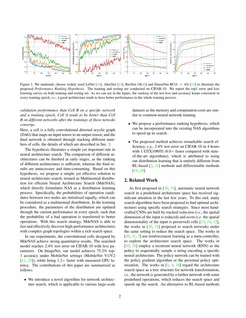
Indeed, most NAS methods [31, 17] perform the per-formance estimation using standard training and validationover each searched architecture, typically, the architecturehas to be trained to converge to get the final evaluation onvalidation set, which is computationally expensive and lim-its the search exploration. However, if the evaluation ofdifferent architectures can be ranked within a few epochs,why do we need to estimate the performance after the neuralnetwork converges? Consider an example in Fig. 1, we ran-domly sample different architectures (LeNet [16], AlexNet[15], ResNet-18 [10] and DenseNet [13]) with different lay-ers, the performance ranking in the training and testing isconsistent (i.e, the performance ranking is ResNet-18 >DenseNet-BC > AlexNet > LeNet on different networksand training epochs). Based on this observation, we statethe following hypothesis for performance ranking:Performance Ranking Hypothesis. If Cell A has higher
Figure 1. We randomly choose widely used LeNet [16], AlexNet [14], ResNet-18[10] and DenseNet-BC(k = 40) [13] to illustrate theproposed Performance Ranking Hypothesis. The training and testing are conducted on CIFAR-10. We report the top1 error and losslearning curves on both training and testing set. As we can see in the figure, the ranking of the test loss and accuracy keeps consistent inevery training epoch, i.e., a good architecture tends to have better performance in the whole training process.
validation performance than Cell B on a specific networkand a training epoch, Cell A tends to be better than CellB on different networks after the trainings of these netwoksconverge.Here, a cell is a fully convolutional directed acyclic graph(DAG) that maps an input tensor to an output tensor, and thefinal network is obtained through stacking different num-bers of cells, the details of which are described in Sec. 3.
The hypothesis illustrates a simple yet important rule inneural architecture search. The comparison of different ar-chitectures can be finished at early stages, as the rankingof different architectures is sufficient, whereas the final re-sults are unnecessary and time-consuming. Based on thishypothesis, we propose a simple yet effective solution toneural architecture search, termed as Multinomial distribu-tion for efficient Neural Architecture Search (MdeNAS),which directly formulates NAS as a distribution learningprocess. Specifically, the probabilities of operation candi-dates between two nodes are initialized equally, which canbe considered as a multinomial distribution. In the learningprocedure, the parameters of the distribution are updatedthrough the current performance in every epoch, such thatthe probability of a bad operation is transferred to betteroperations. With this search strategy, MdeNAS is able tofast and effectively discover high-performance architectureswith complex graph topologies within a rich search space.
In our experiments, the convolutional cells designed byMdeNAS achieve strong quantitative results. The searchedmodel reaches 2.4% test error on CIFAR-10 with less pa-rameters. On ImageNet, our model achieves 75.2% top-1 accuracy under MobileNet settings (MobileNet V1/V2[11, 25]), while being 1.2× faster with measured GPU la-tency. The contributions of this paper are summarized asfollows:
• We introduce a novel algorithm for network architec-ture search, which is applicable to various large-scale
datasets as the memory and computation costs are sim-ilar to common neural network training.
• We propose a performance ranking hypothesis, whichcan be incorporated into the existing NAS algorithmsto speed up its search.
• The proposed method achieves remarkable search ef-ficiency, e.g., 2.4% test error on CIFAR-10 in 4 hourswith 1 GTX1080Ti (6.0× faster compared with state-of-the-art algorithms), which is attributed to usingour distribution learning that is entirely different fromRL-based [2, 31] methods and differentiable methods[19, 28].
2. Related WorkAs first proposed in [30, 31], automatic neural network
search in a predefined architecture space has received sig-nificant attention in the last few years. To this end, manysearch algorithms have been proposed to find optimal archi-tectures using specific search strategies. Since most hand-crafted CNNs are built by stacked reduction (i.e., the spatialdimension of the input is reduced) and norm (i.e. the spatialdimensionality of the input is preserved) cells [13, 10, 12],the works in [30, 31] proposed to search networks underthe same setting to reduce the search space. The works in[30, 31, 2] use reinforcement learning as a meta-controller,to explore the architecture search space. The works in[30, 31] employ a recurrent neural network (RNN) as thepolicy to sequentially sample a string encoding a specificneural architecture. The policy network can be trained withthe policy gradient algorithm or the proximal policy opti-mization. The works in [3, 4, 18] regard the architecturesearch space as a tree structure for network transformation,i.e., the network is generated by a farther network with somepredefined operations, which reduces the search space andspeeds up the search. An alternative to RL-based methods
2
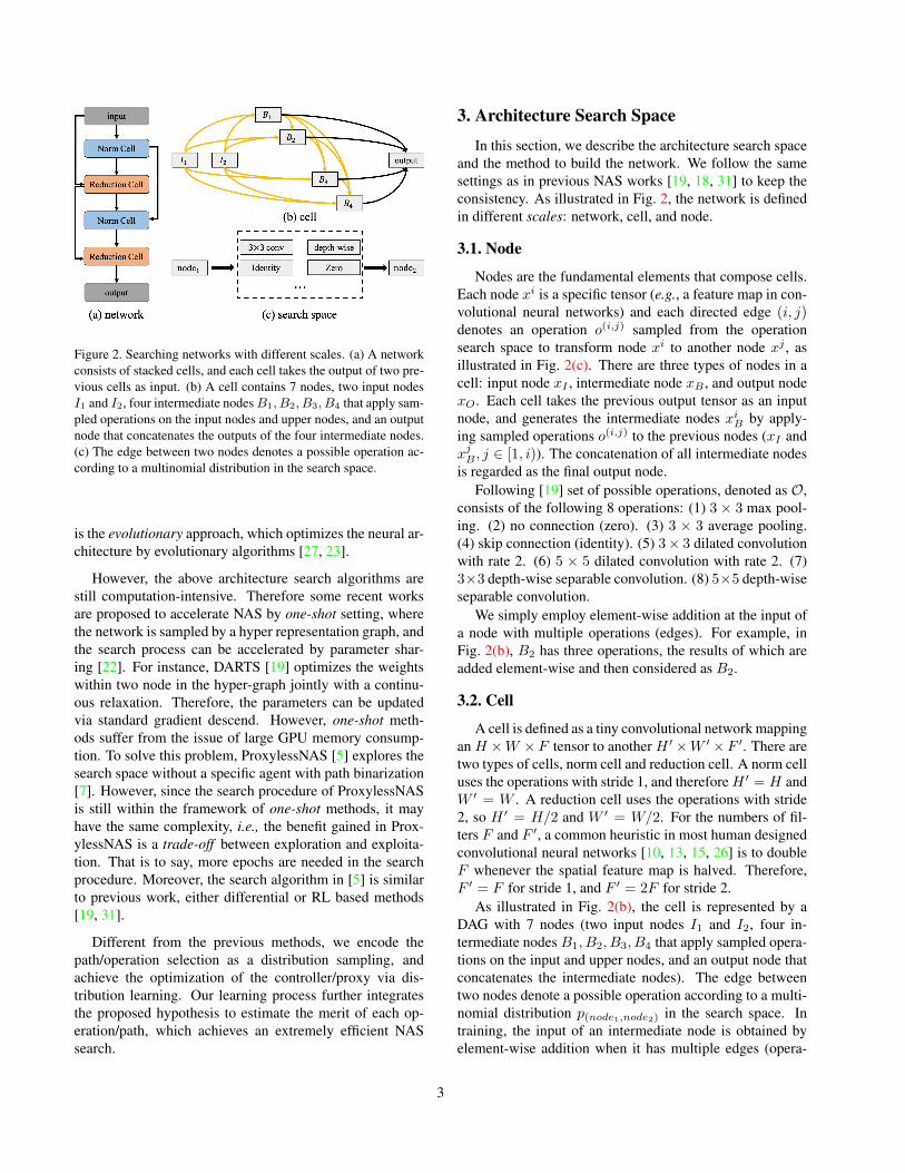
Figure 2. Searching networks with different scales. (a) A networkconsists of stacked cells, and each cell takes the output of two pre-vious cells as input. (b) A cell contains 7 nodes, two input nodesI1 and I2, four intermediate nodesB1, B2, B3, B4 that apply sam-pled operations on the input nodes and upper nodes, and an outputnode that concatenates the outputs of the four intermediate nodes.(c) The edge between two nodes denotes a possible operation ac-cording to a multinomial distribution in the search space.
is the evolutionary approach, which optimizes the neural ar-chitecture by evolutionary algorithms [27, 23].
However, the above architecture search algorithms arestill computation-intensive. Therefore some recent worksare proposed to accelerate NAS by one-shot setting, wherethe network is sampled by a hyper representation graph, andthe search process can be accelerated by parameter shar-ing [22]. For instance, DARTS [19] optimizes the weightswithin two node in the hyper-graph jointly with a continu-ous relaxation. Therefore, the parameters can be updatedvia standard gradient descend. However, one-shot meth-ods suffer from the issue of large GPU memory consump-tion. To solve this problem, ProxylessNAS [5] explores thesearch space without a specific agent with path binarization[7]. However, since the search procedure of ProxylessNASis still within the framework of one-shot methods, it mayhave the same complexity, i.e., the benefit gained in Prox-ylessNAS is a trade-off between exploration and exploita-tion. That is to say, more epochs are needed in the searchprocedure. Moreover, the search algorithm in [5] is similarto previous work, either differential or RL based methods[19, 31].
Different from the previous methods, we encode thepath/operation selection as a distribution sampling, andachieve the optimization of the controller/proxy via dis-tribution learning. Our learning process further integratesthe proposed hypothesis to estimate the merit of each op-eration/path, which achieves an extremely efficient NASsearch.
3. Architecture Search Space
In this section, we describe the architecture search spaceand the method to build the network. We follow the samesettings as in previous NAS works [19, 18, 31] to keep theconsistency. As illustrated in Fig. 2, the network is definedin different scales: network, cell, and node.
3.1. Node
Nodes are the fundamental elements that compose cells.Each node xi is a specific tensor (e.g., a feature map in con-volutional neural networks) and each directed edge (i, j)denotes an operation o(i,j) sampled from the operationsearch space to transform node xi to another node xj , asillustrated in Fig. 2(c). There are three types of nodes in acell: input node xI , intermediate node xB , and output nodexO. Each cell takes the previous output tensor as an inputnode, and generates the intermediate nodes xiB by apply-ing sampled operations o(i,j) to the previous nodes (xI andxjB , j ∈ [1, i)). The concatenation of all intermediate nodesis regarded as the final output node.
Following [19] set of possible operations, denoted as O,consists of the following 8 operations: (1) 3× 3 max pool-ing. (2) no connection (zero). (3) 3 × 3 average pooling.(4) skip connection (identity). (5) 3× 3 dilated convolutionwith rate 2. (6) 5 × 5 dilated convolution with rate 2. (7)3×3 depth-wise separable convolution. (8) 5×5 depth-wiseseparable convolution.
We simply employ element-wise addition at the input ofa node with multiple operations (edges). For example, inFig. 2(b), B2 has three operations, the results of which areadded element-wise and then considered as B2.
3.2. Cell
A cell is defined as a tiny convolutional network mappingan H ×W ×F tensor to another H ′ ×W ′ ×F ′. There aretwo types of cells, norm cell and reduction cell. A norm celluses the operations with stride 1, and thereforeH ′ = H andW ′ = W . A reduction cell uses the operations with stride2, so H ′ = H/2 and W ′ = W/2. For the numbers of fil-ters F and F ′, a common heuristic in most human designedconvolutional neural networks [10, 13, 15, 26] is to doubleF whenever the spatial feature map is halved. Therefore,F ′ = F for stride 1, and F ′ = 2F for stride 2.
As illustrated in Fig. 2(b), the cell is represented by aDAG with 7 nodes (two input nodes I1 and I2, four in-termediate nodes B1, B2, B3, B4 that apply sampled opera-tions on the input and upper nodes, and an output node thatconcatenates the intermediate nodes). The edge betweentwo nodes denote a possible operation according to a multi-nomial distribution p(node1,node2) in the search space. Intraining, the input of an intermediate node is obtained byelement-wise addition when it has multiple edges (opera-
3
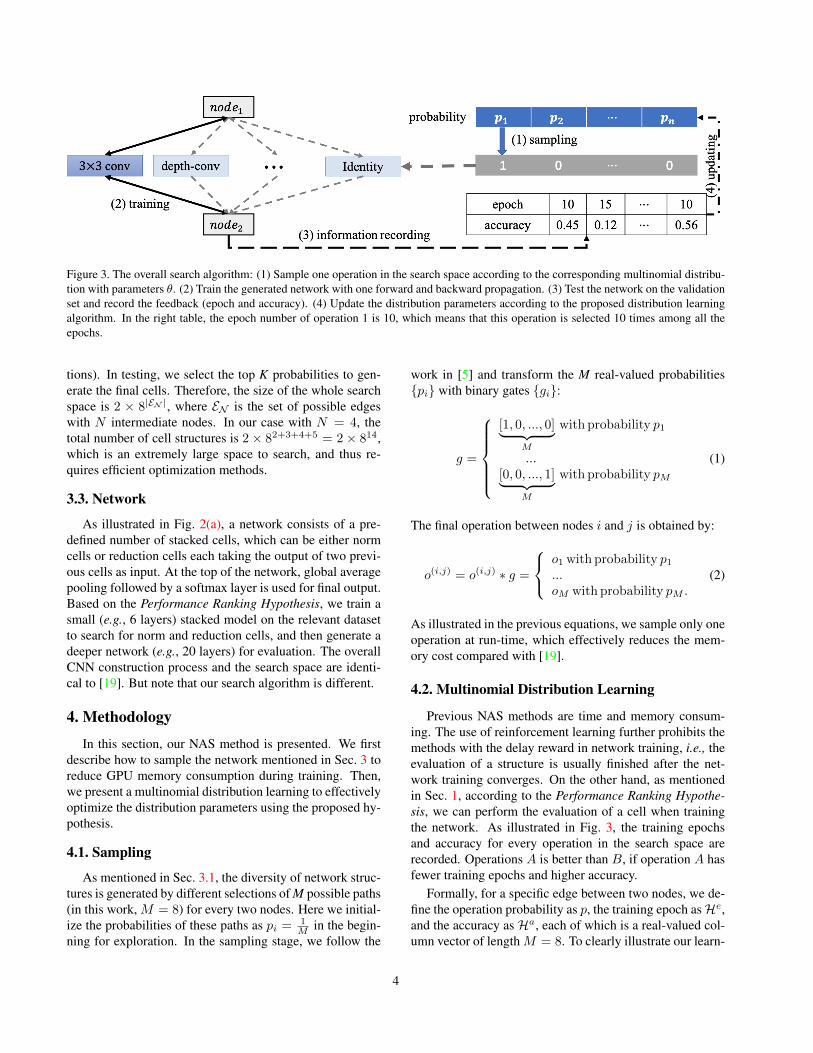
Figure 3. The overall search algorithm: (1) Sample one operation in the search space according to the corresponding multinomial distribu-tion with parameters θ. (2) Train the generated network with one forward and backward propagation. (3) Test the network on the validationset and record the feedback (epoch and accuracy). (4) Update the distribution parameters according to the proposed distribution learningalgorithm. In the right table, the epoch number of operation 1 is 10, which means that this operation is selected 10 times among all theepochs.
tions). In testing, we select the top K probabilities to gen-erate the final cells. Therefore, the size of the whole searchspace is 2 × 8|EN |, where EN is the set of possible edgeswith N intermediate nodes. In our case with N = 4, thetotal number of cell structures is 2× 82+3+4+5 = 2 × 814,which is an extremely large space to search, and thus re-quires efficient optimization methods.
3.3. Network
As illustrated in Fig. 2(a), a network consists of a pre-defined number of stacked cells, which can be either normcells or reduction cells each taking the output of two previ-ous cells as input. At the top of the network, global averagepooling followed by a softmax layer is used for final output.Based on the Performance Ranking Hypothesis, we train asmall (e.g., 6 layers) stacked model on the relevant datasetto search for norm and reduction cells, and then generate adeeper network (e.g., 20 layers) for evaluation. The overallCNN construction process and the search space are identi-cal to [19]. But note that our search algorithm is different.
4. Methodology
In this section, our NAS method is presented. We firstdescribe how to sample the network mentioned in Sec. 3 toreduce GPU memory consumption during training. Then,we present a multinomial distribution learning to effectivelyoptimize the distribution parameters using the proposed hy-pothesis.
4.1. Sampling
As mentioned in Sec. 3.1, the diversity of network struc-tures is generated by different selections of M possible paths(in this work, M = 8) for every two nodes. Here we initial-ize the probabilities of these paths as pi = 1
M in the begin-ning for exploration. In the sampling stage, we follow the
work in [5] and transform the M real-valued probabilities{pi} with binary gates {gi}:
g =
[1, 0, ..., 0]︸ ︷︷ ︸
M
with probability p1
...[0, 0, ..., 1]︸ ︷︷ ︸
M
with probability pM
(1)
The final operation between nodes i and j is obtained by:
o(i,j) = o(i,j) ∗ g =
o1 with probability p1...oM with probability pM .
(2)
As illustrated in the previous equations, we sample only oneoperation at run-time, which effectively reduces the mem-ory cost compared with [19].
4.2. Multinomial Distribution Learning
Previous NAS methods are time and memory consum-ing. The use of reinforcement learning further prohibits themethods with the delay reward in network training, i.e., theevaluation of a structure is usually finished after the net-work training converges. On the other hand, as mentionedin Sec. 1, according to the Performance Ranking Hypothe-sis, we can perform the evaluation of a cell when trainingthe network. As illustrated in Fig. 3, the training epochsand accuracy for every operation in the search space arerecorded. Operations A is better than B, if operation A hasfewer training epochs and higher accuracy.
Formally, for a specific edge between two nodes, we de-fine the operation probability as p, the training epoch asHe,and the accuracy as Ha, each of which is a real-valued col-umn vector of lengthM = 8. To clearly illustrate our learn-
4
ing method, we further define the differential of epoch as:
∆He =
(~1×He1 −He)T...
(~1×HeM −He)T
, (3)
and the differential of accuracy as:
∆Ha =
(~1×Ha1 −Ha)T
...
(~1×HaM −Ha)T
, (4)
where~1 is a column vector with length 8 and all its elementsbeing 1, ∆He and ∆Ha are 8×8 matrices, where ∆Hei,j =Hei − Hej ,∆Hai,j = Hai − Haj . After one epoch training,the corresponding variables He, Ha, ∆He and ∆Ha arecalculated by the evaluation results. The parameters of themultinomial distribution can be updated through:
pi ← pi + α ∗ (∑j
1(∆Hei,j < 0,∆Hai,j > 0)−
∑j
1(∆Hei,j > 0,∆Hai,j < 0)),(5)
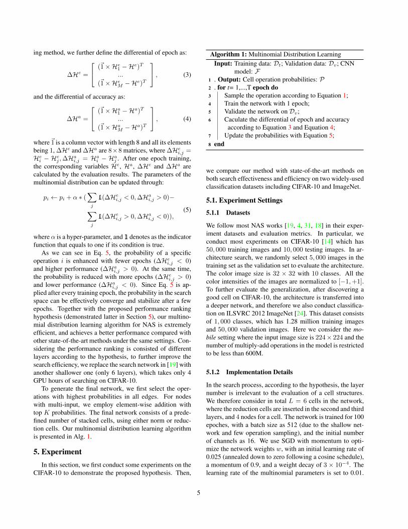
where α is a hyper-parameter, and 1 denotes as the indicatorfunction that equals to one if its condition is true.
As we can see in Eq. 5, the probability of a specificoperation i is enhanced with fewer epochs (∆Hei,j < 0)and higher performance (∆Hai,j > 0). At the same time,the probability is reduced with more epochs (∆Hei,j > 0)and lower performance (∆Hai,j < 0). Since Eq. 5 is ap-plied after every training epoch, the probability in the searchspace can be effectively converge and stabilize after a fewepochs. Together with the proposed performance rankinghypothesis (demonstrated latter in Section 5), our multino-mial distribution learning algorithm for NAS is extremelyefficient, and achieves a better performance compared withother state-of-the-art methods under the same settings. Con-sidering the performance ranking is consisted of differentlayers according to the hypothesis, to further improve thesearch efficiency, we replace the search network in [19] withanother shallower one (only 6 layers), which takes only 4GPU hours of searching on CIFAR-10.
To generate the final network, we first select the oper-ations with highest probabilities in all edges. For nodeswith multi-input, we employ element-wise addition withtop K probabilities. The final network consists of a prede-fined number of stacked cells, using either norm or reduc-tion cells. Our multinomial distribution learning algorithmis presented in Alg. 1.
5. ExperimentIn this section, we first conduct some experiments on the
CIFAR-10 to demonstrate the proposed hypothesis. Then,
Algorithm 1: Multinomial Distribution LearningInput: Training data: Dt; Validation data: Dv; CNN
model: F1 . Output: Cell operation probabilities: P2 . for t= 1,...,T epoch do3 Sample the operation according to Equation 1;4 Train the network with 1 epoch;5 Validate the network on Dv;6 Caculate the differential of epoch and accuracy
according to Equation 3 and Equation 4;7 Update the probabilities with Equation 5;8 end
we compare our method with state-of-the-art methods onboth search effectiveness and efficiency on two widely-usedclassification datasets including CIFAR-10 and ImageNet.
5.1. Experiment Settings
5.1.1 Datasets
We follow most NAS works [19, 4, 31, 18] in their exper-iment datasets and evaluation metrics. In particular, weconduct most experiments on CIFAR-10 [14] which has50, 000 training images and 10, 000 testing images. In ar-chitecture search, we randomly select 5, 000 images in thetraining set as the validation set to evaluate the architecture.The color image size is 32 × 32 with 10 classes. All thecolor intensities of the images are normalized to [−1,+1].To further evaluate the generalization, after discovering agood cell on CIFAR-10, the architecture is transferred intoa deeper network, and therefore we also conduct classifica-tion on ILSVRC 2012 ImageNet [24]. This dataset consistsof 1, 000 classes, which has 1.28 million training imagesand 50, 000 validation images. Here we consider the mo-bile setting where the input image size is 224× 224 and thenumber of multiply-add operations in the model is restrictedto be less than 600M.
5.1.2 Implementation Details
In the search process, according to the hypothesis, the layernumber is irrelevant to the evaluation of a cell structures.We therefore consider in total L = 6 cells in the network,where the reduction cells are inserted in the second and thirdlayers, and 4 nodes for a cell. The network is trained for 100epoches, with a batch size as 512 (due to the shallow net-work and few operation sampling), and the initial numberof channels as 16. We use SGD with momentum to opti-mize the network weights w, with an initial learning rate of0.025 (annealed down to zero following a cosine schedule),a momentum of 0.9, and a weight decay of 3 × 10⁻⁴. Thelearning rate of the multinomial parameters is set to 0.01.
5
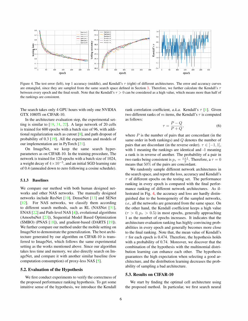
Figure 4. The test error (left), top 1 accuracy (middle), and Kendall’s τ (right) of different architectures. The error and accuracy curvesare entangled, since they are sampled from the same search space defined in Section 3. Therefore, we further calculate the Kendall’s τbetween every epoch and the final result. Note that the Kendall’s τ > 0 can be considered as a high value, which means more than half ofthe rankings are consistent.
The search takes only 4 GPU hours with only one NVIDIAGTX 1080Ti on CIFAR-10.
In the architecture evaluation step, the experimental set-ting is similar to [19, 31, 22]. A large network of 20 cellsis trained for 600 epochs with a batch size of 96, with addi-tional regularization such as cutout [8], and path dropout ofprobability of 0.3 [19]. All the experiments and models ofour implementation are in PyTorch [21].
On ImageNet, we keep the same search hyper-parameters as on CIFAR-10. In the training procedure, Thenetwork is trained for 120 epochs with a batch size of 1024,a weight decay of 4×10⁻⁵, and an initial SGD learning rateof 0.4 (annealed down to zero following a cosine schedule).
5.1.3 Baselines
We compare our method with both human designed net-works and other NAS networks. The manually designednetworks include ResNet [10], DenseNet [13] and SENet[12]. For NAS networks, we classify them accordingto different search methods, such as RL (NASNet [31],ENAS [22] and Path-level NAS [4]), evolutional algorithms(AmoebaNet [23]), Sequential Model Based Optimization(SMBO) (PNAS [18]), and gradient-based (DARTS [19]).We further compare our method under the mobile setting onImageNet to demonstrate the generalization. The best archi-tecture generated by our algorithm on CIFAR-10 is trans-ferred to ImageNet, which follows the same experimentalsetting as the works mentioned above. Since our algorithmtakes less time and memory, we also directly search on Im-ageNet, and compare it with another similar baseline (lowcomputation consumption) of proxy-less NAS [5].
5.2. Evaluation of the Hypothesis
We first conduct experiments to verify the correctness ofthe proposed performance ranking hypothesis. To get someintuitive sense of the hypothesis, we introduce the Kendall
rank correlation coefficient, a.k.a. Kendall’s τ [1]. Giventwo different ranks of m items, the Kendall’s τ is computedas follows:
τ =P −QP +Q
, (6)
where P is the number of pairs that are concordant (in thesame order in both rankings) and Q denotes the number ofpairs that are discordant (in the reverse order). τ ∈ [−1, 1],with 1 meaning the rankings are identical and -1 meaninga rank is in reverse of another. The probability of a pair intwo ranks being consistent is pτ = τ+1
2 . Therefore, a τ = 0means that 50% of the pairs are concordant.
We randomly sample different network architectures inthe search space, and report the loss, accuracy and Kendall’sτ of different epochs on the testing set. The performanceranking in every epoch is compared with the final perfor-mance ranking of different network architectures. As il-lustrated in Fig. 4, the accuracy and loss are hardly distin-guished due to the homogeneity of the sampled networks,i.e., all the networks are generated from the same space. Onthe other hand, the Kendall coefficient keeps a high value(τ > 0, pτ > 0.5) in most epochs, generally approaching1 as the number of epochs increases. It indicates that thearchitecture evaluation ranking has highly convincing prob-abilities in every epoch and generally becomes more closeto the final ranking. Note that, the mean value of Kendall’sτ for each epoch is 0.474. Therefore, the hypothesis holdswith a probability of 0.74. Moreover, we discover that thecombination of the hypothesis with the multinomial distri-bution learning can enhance each other. The hypothesisguarantees the high expectation when selecting a good ar-chitecture, and the distribution learning decreases the prob-ability of sampling a bad architecture.
5.3. Results on CIFAR-10
We start by finding the optimal cell architecture usingthe proposed method. In particular, we first search neural
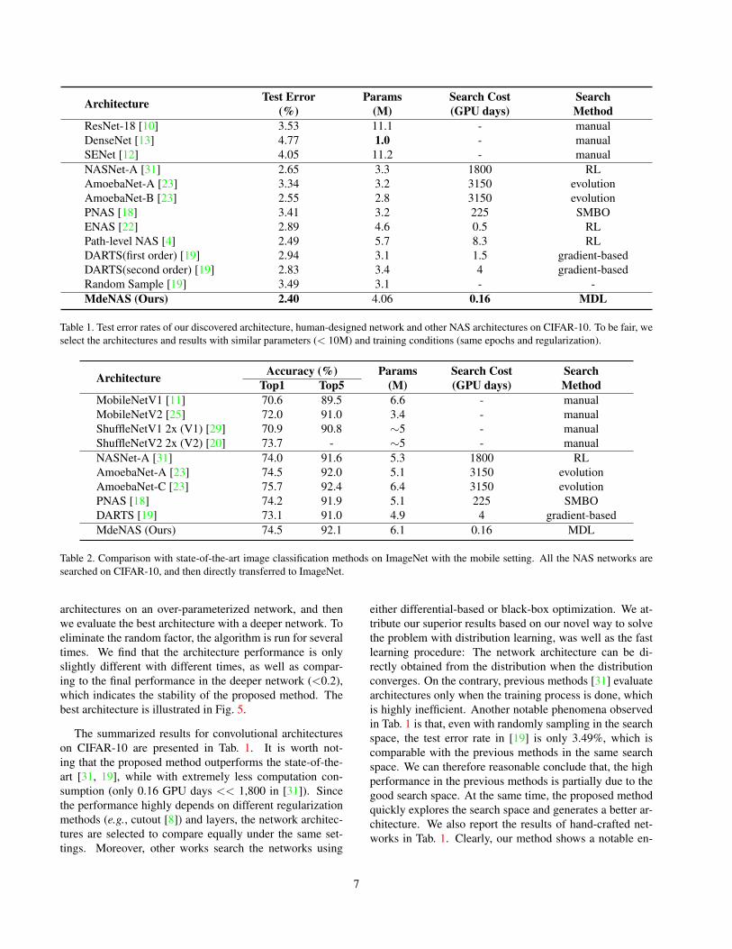
Table 1. Test error rates of our discovered architecture, human-designed network and other NAS architectures on CIFAR-10. To be fair, weselect the architectures and results with similar parameters (< 10M) and training conditions (same epochs and regularization).
Table 2. Comparison with state-of-the-art image classification methods on ImageNet with the mobile setting. All the NAS networks aresearched on CIFAR-10, and then directly transferred to ImageNet.
architectures on an over-parameterized network, and thenwe evaluate the best architecture with a deeper network. Toeliminate the random factor, the algorithm is run for severaltimes. We find that the architecture performance is onlyslightly different with different times, as well as compar-ing to the final performance in the deeper network (<0.2),which indicates the stability of the proposed method. Thebest architecture is illustrated in Fig. 5.
The summarized results for convolutional architectureson CIFAR-10 are presented in Tab. 1. It is worth not-ing that the proposed method outperforms the state-of-the-art [31, 19], while with extremely less computation con-sumption (only 0.16 GPU days << 1,800 in [31]). Sincethe performance highly depends on different regularizationmethods (e.g., cutout [8]) and layers, the network architec-tures are selected to compare equally under the same set-tings. Moreover, other works search the networks using
either differential-based or black-box optimization. We at-tribute our superior results based on our novel way to solvethe problem with distribution learning, was well as the fastlearning procedure: The network architecture can be di-rectly obtained from the distribution when the distributionconverges. On the contrary, previous methods [31] evaluatearchitectures only when the training process is done, whichis highly inefficient. Another notable phenomena observedin Tab. 1 is that, even with randomly sampling in the searchspace, the test error rate in [19] is only 3.49%, which iscomparable with the previous methods in the same searchspace. We can therefore reasonable conclude that, the highperformance in the previous methods is partially due to thegood search space. At the same time, the proposed methodquickly explores the search space and generates a better ar-chitecture. We also report the results of hand-crafted net-works in Tab. 1. Clearly, our method shows a notable en-
7
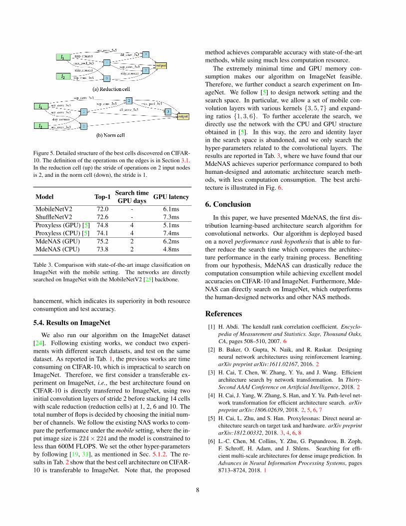
Figure 5. Detailed structure of the best cells discovered on CIFAR-10. The definition of the operations on the edges is in Section 3.1.In the reduction cell (up) the stride of operations on 2 input nodesis 2, and in the norm cell (down), the stride is 1.
Table 3. Comparison with state-of-the-art image classification onImageNet with the mobile setting. The networks are directlysearched on ImageNet with the MobileNetV2 [25] backbone.
hancement, which indicates its superiority in both resourceconsumption and test accuracy.
5.4. Results on ImageNet
We also run our algorithm on the ImageNet dataset[24]. Following existing works, we conduct two experi-ments with different search datasets, and test on the samedataset. As reported in Tab. 1, the previous works are timeconsuming on CIFAR-10, which is impractical to search onImageNet. Therefore, we first consider a transferable ex-periment on ImageNet, i.e., the best architecture found onCIFAR-10 is directly transferred to ImageNet, using twoinitial convolution layers of stride 2 before stacking 14 cellswith scale reduction (reduction cells) at 1, 2, 6 and 10. Thetotal number of flops is decided by choosing the initial num-ber of channels. We follow the existing NAS works to com-pare the performance under the mobile setting, where the in-put image size is 224× 224 and the model is constrained toless than 600M FLOPS. We set the other hyper-parametersby following [19, 31], as mentioned in Sec. 5.1.2. The re-sults in Tab. 2 show that the best cell architecture on CIFAR-10 is transferable to ImageNet. Note that, the proposed
method achieves comparable accuracy with state-of-the-artmethods, while using much less computation resource.
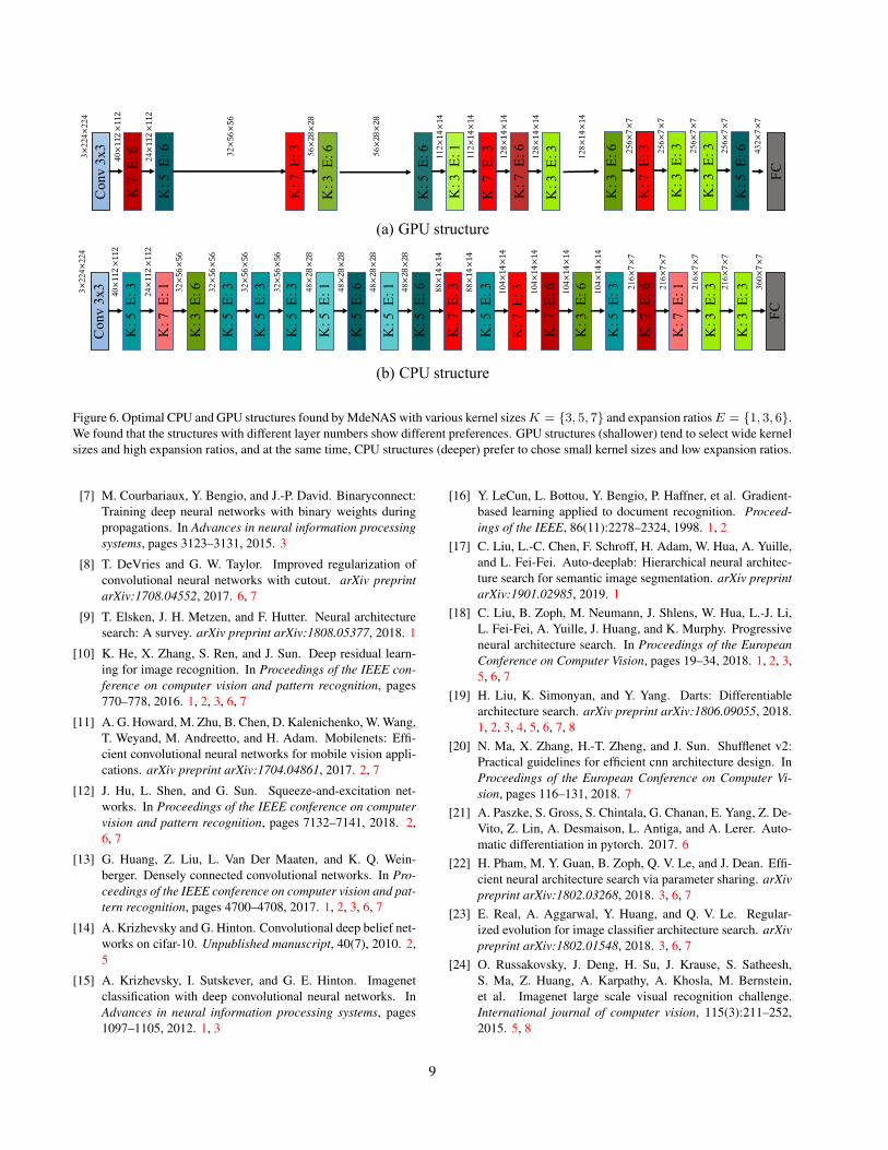
The extremely minimal time and GPU memory con-sumption makes our algorithm on ImageNet feasible.Therefore, we further conduct a search experiment on Im-ageNet. We follow [5] to design network setting and thesearch space. In particular, we allow a set of mobile con-volution layers with various kernels {3, 5, 7} and expand-ing ratios {1, 3, 6}. To further accelerate the search, wedirectly use the network with the CPU and GPU structureobtained in [5]. In this way, the zero and identity layerin the search space is abandoned, and we only search thehyper-parameters related to the convolutional layers. Theresults are reported in Tab. 3, where we have found that ourMdeNAS achieves superior performance compared to bothhuman-designed and automatic architecture search meth-ods, with less computation consumption. The best archi-tecture is illustrated in Fig. 6.
6. Conclusion
In this paper, we have presented MdeNAS, the first dis-tribution learning-based architecture search algorithm forconvolutional networks. Our algorithm is deployed basedon a novel performance rank hypothesis that is able to fur-ther reduce the search time which compares the architec-ture performance in the early training process. Benefitingfrom our hypothesis, MdeNAS can drastically reduce thecomputation consumption while achieving excellent modelaccuracies on CIFAR-10 and ImageNet. Furthermore, Mde-NAS can directly search on ImageNet, which outperformsthe human-designed networks and other NAS methods.
References[1] H. Abdi. The kendall rank correlation coefficient. Encyclo-
pedia of Measurement and Statistics. Sage, Thousand Oaks,CA, pages 508–510, 2007. 6
[2] B. Baker, O. Gupta, N. Naik, and R. Raskar. Designingneural network architectures using reinforcement learning.arXiv preprint arXiv:1611.02167, 2016. 2
[3] H. Cai, T. Chen, W. Zhang, Y. Yu, and J. Wang. Efficientarchitecture search by network transformation. In Thirty-Second AAAI Conference on Artificial Intelligence, 2018. 2
[4] H. Cai, J. Yang, W. Zhang, S. Han, and Y. Yu. Path-level net-work transformation for efficient architecture search. arXivpreprint arXiv:1806.02639, 2018. 2, 5, 6, 7
[5] H. Cai, L. Zhu, and S. Han. Proxylessnas: Direct neural ar-chitecture search on target task and hardware. arXiv preprintarXiv:1812.00332, 2018. 3, 4, 6, 8
[6] L.-C. Chen, M. Collins, Y. Zhu, G. Papandreou, B. Zoph,F. Schroff, H. Adam, and J. Shlens. Searching for effi-cient multi-scale architectures for dense image prediction. InAdvances in Neural Information Processing Systems, pages8713–8724, 2018. 1
8
K:7
E:6
K: 5
E:6
K: 7
E:3
Con
v 3x
3
K: 3
E:6
K: 3
E:6
K: 7
E:3
K: 7
E:6
K: 5
E:6
FC
K: 5
E:6
K: 3
E:3
K: 7
E:3
K: 3
E:3
K: 3
E:1
FC
Con
v 3x
3
K: 5
E:3
K: 7
E:1
K: 3
E:6
K: 5
E:3
K: 3
E:6
K: 5
E:3
K: 7
E:6
K: 7
E:3
K: 5
E:6
K: 3
E:3
K: 7
E:1
K: 5
E:1
K: 3
E:3
K: 5
E:3
K: 7
E:6
K: 7
E:3
K: 5
E:3
K: 5
E:3
K: 5
E:1
K: 5
E:6
(a) GPU structure
(b) CPU structure
K: 3
E:33×
224×
224
40×112×112
24×112×112
3×22
4×22
4
40×112×112
24×112×112
32×56×56
32×56×56
32×56×56
32×56×56
48×28×28
48×28×28
48×28×28
48×28×28
88×14×14
88×14×14
104×14×14
104×14×14
104×14×14
104×14×14
216×7×7
216×7×7
216×7×7
216×7×7
360×7×7
32×56×56
56×28×28
56×28×28
112×14×14
112×14×14
128×14×14
128×14×14
256×7×7
128×14×14
256×7×7
256×7×7
256×7×7
432×7×7
Figure 6. Optimal CPU and GPU structures found by MdeNAS with various kernel sizesK = {3, 5, 7} and expansion ratiosE = {1, 3, 6}.We found that the structures with different layer numbers show different preferences. GPU structures (shallower) tend to select wide kernelsizes and high expansion ratios, and at the same time, CPU structures (deeper) prefer to chose small kernel sizes and low expansion ratios.
[7] M. Courbariaux, Y. Bengio, and J.-P. David. Binaryconnect:Training deep neural networks with binary weights duringpropagations. In Advances in neural information processingsystems, pages 3123–3131, 2015. 3
[8] T. DeVries and G. W. Taylor. Improved regularization ofconvolutional neural networks with cutout. arXiv preprintarXiv:1708.04552, 2017. 6, 7
[9] T. Elsken, J. H. Metzen, and F. Hutter. Neural architecturesearch: A survey. arXiv preprint arXiv:1808.05377, 2018. 1
[10] K. He, X. Zhang, S. Ren, and J. Sun. Deep residual learn-ing for image recognition. In Proceedings of the IEEE con-ference on computer vision and pattern recognition, pages770–778, 2016. 1, 2, 3, 6, 7
[11] A. G. Howard, M. Zhu, B. Chen, D. Kalenichenko, W. Wang,T. Weyand, M. Andreetto, and H. Adam. Mobilenets: Effi-cient convolutional neural networks for mobile vision appli-cations. arXiv preprint arXiv:1704.04861, 2017. 2, 7
[12] J. Hu, L. Shen, and G. Sun. Squeeze-and-excitation net-works. In Proceedings of the IEEE conference on computervision and pattern recognition, pages 7132–7141, 2018. 2,6, 7
[13] G. Huang, Z. Liu, L. Van Der Maaten, and K. Q. Wein-berger. Densely connected convolutional networks. In Pro-ceedings of the IEEE conference on computer vision and pat-tern recognition, pages 4700–4708, 2017. 1, 2, 3, 6, 7
[14] A. Krizhevsky and G. Hinton. Convolutional deep belief net-works on cifar-10. Unpublished manuscript, 40(7), 2010. 2,5
[15] A. Krizhevsky, I. Sutskever, and G. E. Hinton. Imagenetclassification with deep convolutional neural networks. InAdvances in neural information processing systems, pages1097–1105, 2012. 1, 3
[16] Y. LeCun, L. Bottou, Y. Bengio, P. Haffner, et al. Gradient-based learning applied to document recognition. Proceed-ings of the IEEE, 86(11):2278–2324, 1998. 1, 2
[17] C. Liu, L.-C. Chen, F. Schroff, H. Adam, W. Hua, A. Yuille,and L. Fei-Fei. Auto-deeplab: Hierarchical neural architec-ture search for semantic image segmentation. arXiv preprintarXiv:1901.02985, 2019. 1
[18] C. Liu, B. Zoph, M. Neumann, J. Shlens, W. Hua, L.-J. Li,L. Fei-Fei, A. Yuille, J. Huang, and K. Murphy. Progressiveneural architecture search. In Proceedings of the EuropeanConference on Computer Vision, pages 19–34, 2018. 1, 2, 3,5, 6, 7
[19] H. Liu, K. Simonyan, and Y. Yang. Darts: Differentiablearchitecture search. arXiv preprint arXiv:1806.09055, 2018.1, 2, 3, 4, 5, 6, 7, 8
[20] N. Ma, X. Zhang, H.-T. Zheng, and J. Sun. Shufflenet v2:Practical guidelines for efficient cnn architecture design. InProceedings of the European Conference on Computer Vi-sion, pages 116–131, 2018. 7
[21] A. Paszke, S. Gross, S. Chintala, G. Chanan, E. Yang, Z. De-Vito, Z. Lin, A. Desmaison, L. Antiga, and A. Lerer. Auto-matic differentiation in pytorch. 2017. 6
[22] H. Pham, M. Y. Guan, B. Zoph, Q. V. Le, and J. Dean. Effi-cient neural architecture search via parameter sharing. arXivpreprint arXiv:1802.03268, 2018. 3, 6, 7
[23] E. Real, A. Aggarwal, Y. Huang, and Q. V. Le. Regular-ized evolution for image classifier architecture search. arXivpreprint arXiv:1802.01548, 2018. 3, 6, 7
[24] O. Russakovsky, J. Deng, H. Su, J. Krause, S. Satheesh,S. Ma, Z. Huang, A. Karpathy, A. Khosla, M. Bernstein,et al. Imagenet large scale visual recognition challenge.International journal of computer vision, 115(3):211–252,2015. 5, 8
9
[25] M. Sandler, A. Howard, M. Zhu, A. Zhmoginov, and L.-C.Chen. Mobilenetv2: Inverted residuals and linear bottle-necks. In Proceedings of the IEEE Conference on ComputerVision and Pattern Recognition, pages 4510–4520, 2018. 2,7, 8
[26] K. Simonyan and A. Zisserman. Very deep convolutionalnetworks for large-scale image recognition. arXiv preprintarXiv:1409.1556, 2014. 3
[27] L. Xie and A. Yuille. Genetic cnn. In Proceedings of theIEEE International Conference on Computer Vision, pages1379–1388, 2017. 3
[28] S. Xie, H. Zheng, C. Liu, and L. Lin. Snas: stochastic neuralarchitecture search. arXiv preprint arXiv:1812.09926, 2018.2
[29] X. Zhang, X. Zhou, M. Lin, and J. Sun. Shufflenet: An ex-tremely efficient convolutional neural network for mobile de-vices. In Proceedings of the IEEE Conference on ComputerVision and Pattern Recognition, pages 6848–6856, 2018. 7
[30] B. Zoph and Q. V. Le. Neural architecture search with rein-forcement learning. arXiv preprint arXiv:1611.01578, 2016.1, 2
[31] B. Zoph, V. Vasudevan, J. Shlens, and Q. V. Le. Learningtransferable architectures for scalable image recognition. InProceedings of the IEEE conference on computer vision andpattern recognition, pages 8697–8710, 2018. 1, 2, 3, 5, 6, 7,8