31
9/29/00 BYU Wireless Communications 1 Multipath Interference Characterization in Wireless Communication Systems Michael Rice BYU Wireless Communications Lab 166

9/29/00 BYU Wireless Communications 1
Multipath Interference Characterizationin Wireless Communication Systems
Michael Rice
BYU Wireless Communications Lab
166
9/29/00 BYU Wireless Communications 2
Multipath Propagation
• Multiple paths between transmitter and receiver
• Constructive/destructive interference
• Dramatic changes in received signal amplitude and phase as a result ofsmall changes (λ/2) in the spatial separation between a receiver andtransmitter.
• For Mobile radio (cellular, PCS, etc) the channel is time-variantbecause motion between the transmitter and receiver results inpropagation path changes.
• Terms: Rayleigh Fading, Rice Fading, Flat Fading, FrequencySelective Fading, Slow Fading, Fast Fading ….
• What do all these mean?
167
9/29/00 BYU Wireless Communications 3
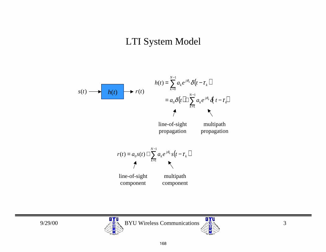
LTI System Model
h(t))(ts )(tr
( )
( ) ( )∑
∑−
=
−
=
−+=
−=
1
10
1
0
)(
N
kk
jk
N
kk
jk
teata
teath
k
k
τδδ
τδ
θ
θ
line-of-sightpropagation
multipathpropagation
( )∑−
=
−+=1
10 )()(
N
kk
jk tseatsatr k τθ
line-of-sightcomponent
multipathcomponent
168
9/29/00 BYU Wireless Communications 4
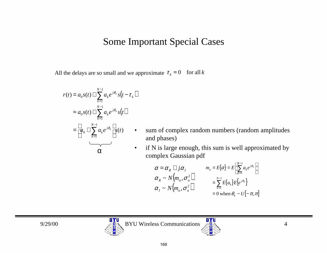
Some Important Special Cases
All the delays are so small and we approximate kk allfor 0≈τ
( )
( )
)(
)(
)()(
1
10
1
10
1
10
tseaa
tseatsa
tseatsatr
N
k
jk
N
k
jk
N
kk
jk
k
k
k
+=
+≈
−+=
∑
∑
∑
−
=
−
=
−
=
θ
θ
θ τ
• sum of complex random numbers (random amplitudesand phases)
• if N is large enough, this sum is well approximated bycomplex Gaussian pdf
α
( )( )2
2
,~
,~
aaI
aaR
IR
mN
mN
j
σασα
ααα += { }
{ } { }[ ]ππθ
α
θ
θ
,~ when 0
1
1
1
1
−=
=
==
∑
∑−
=
−
=
U
eEaE
eaEEm
k
N
k
jk
N
k
jka
k
k
169

9/29/00 BYU Wireless Communications 5
Some Important Special Cases
All the delays are so small and we approximate kk allfor 0≈τ
( )
( )
[ ][ ]
( ) ( ) )(
)(
)(
)(
)(
)()(
220
0
0
1
10
1
10
1
10
tsea
tsja
tsa
tseaa
tseatsa
tseatsatr
jIR
IR
N
k
jk
N
k
jk
N
kk
jk
k
k
k
φ
θ
θ
θ
αα
ααα
τ
++=
++=+=
+=
+≈
−+=
∑
∑
∑
−
=
−
=
−
=
( ) ( ))(
)()(
22
21
220
tseXX
tseatr
j
jIR
φ
φαα
+=
++=
( )201 ,~ aaNX σ ( )2
2 ,0~ aNX σ
170
9/29/00 BYU Wireless Communications 6
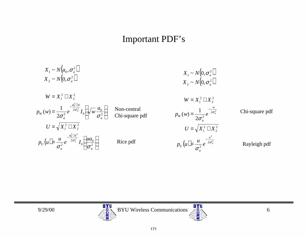
Important PDF’s
( )( )
( )
=
+=
=
+=
+−
+−
20
02
2
22
21
20
02
2
22
21
22
201
2
220
2
20
2
1)(
,0~
,~
a
ua
aU
a
wa
aW
a
a
uaIe
uup
XXU
awIewp
XXW
NX
aNX
a
a
σσ
σσ
σσ
σ
σ Non-centralChi-square pdf
Rice pdf
( )( )
( ) 2
2
2
22
22
21
22
22
21
22
21
2
1)(
,0~
,0~
a
a
u
aU
w
aW
a
a
eu
up
XXU
ewp
XXW
NX
NX
σ
σ
σ
σ
σσ
−
−
=
+=
=
+=
Chi-square pdf
Rayleigh pdf
171

9/29/00 BYU Wireless Communications 7
Back to Some Important Special Cases
All the delays are so small and we approximate kk allfor 0≈τ
( )
( )
( ) ( ) )(
)(
)()(
220
1
10
1
10
tsea
tseatsa
tseatsatr
jIR
N
k
jk
N
kk
jk
k
k
φ
θ
θ
αα
τ
++=
+≈
−+=
∑
∑−
=
−
=
Rice pdf
“Ricean fading”
00 >a
( )
( )
( ) ( ) )(
)(
22
1
1
1
1
tse
tsea
tseatr
jIR
N
k
jk
N
kk
jk
k
k
φ
θ
θ
αα
τ
+=
≈
−=
∑
∑−
=
−
=
Rayleigh pdf
“Rayleigh fading”
00 =a
172

9/29/00 BYU Wireless Communications 8
Some Important Special Cases
All the delays are small and we approximate kk allfor ττ ≈
( )
( )
( ) ( ) ( )ταα
τ
τ
φ
θ
θ
−++=
−+≈
−+=
∑
∑−
=
−
=
tsetsa
tseatsa
tseatsatr
jIR
N
k
jk
N
kk
jk
k
k
220
1
10
1
10
)(
)(
)()(
Rayleigh pdf
“Line-of-sight with Rayleigh Fading”
00 >a
( )
( )
( ) ( ) ( )ταα
τ
τ
φ
θ
θ
−+=
−≈
−=
∑
∑−
=
−
=
tse
tsea
tseatr
jIR
N
k
jk
N
kk
jk
k
k
22
1
1
1
1
)(
Rayleigh pdf
“Rayleigh fading”
00 =a
173

9/29/00 BYU Wireless Communications 9
Multiplicative Fading
In the past two examples, the received signal was of the form
)()( tsFetr jφ=
The fading takes the form of a random attenuation: the transmittedsignal is multiplied by a random value whose envelope is describedby the Rice or Rayleigh pdf.
This is sometimes called multiplicative fading for the obviousreason. It is also called flat fading since all spectral components ins(t) are attenuated by the same value.
174

9/29/00 BYU Wireless Communications 10
An Example
τ1θ
f
2)( fH
( )21 a+
( )21 a−
( ) ( )( )
( ) ( )θτπ
τδδτπθ
θ
−++=
+=−+=
−
faafH
aefH
taetthfj
j
2cos21
1
)(
22
)2(
τ1θ
f
(dB) )(2
fH
( )210 1log10 a+
( )210 1log10 a−
h(t))(ts )(tr
( )fS ( )fR
( )fS
fWW−
( )fR
fWW−
????
?
??
?
175
9/29/00 BYU Wireless Communications 11
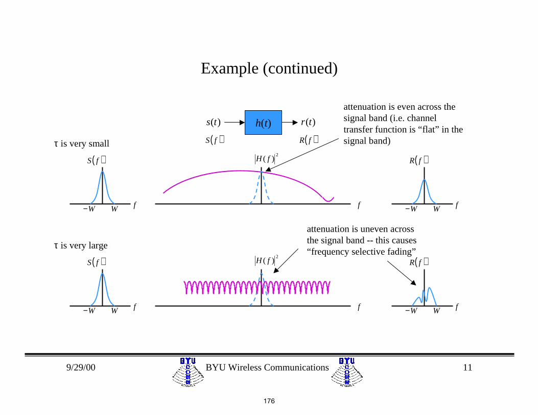
Example (continued)
f
2)( fH( )fS
fWW−
( )fR
fWW−
h(t))(ts )(tr
( )fS ( )fRτ is very small
f
2)( fH( )fS
fWW−
( )fR
fWW−
τ is very large
attenuation is even across thesignal band (i.e. channeltransfer function is “flat” in thesignal band)
attenuation is uneven acrossthe signal band -- this causes“frequency selective fading”
176
9/29/00 BYU Wireless Communications 12
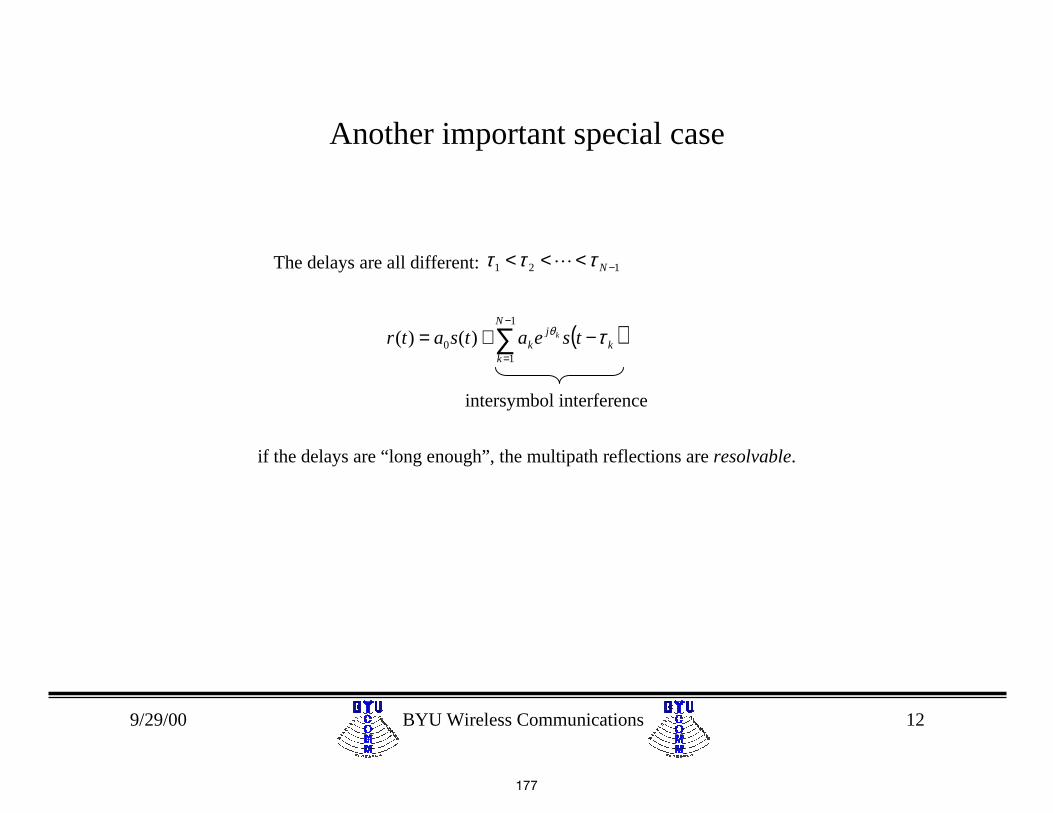
Another important special case
The delays are all different:
( )∑−
=
−+=1
10 )()(
N
kk
jk tseatsatr k τθ
121 −<<< Nτττ L
intersymbol interference
if the delays are “long enough”, the multipath reflections are resolvable.
177

9/29/00 BYU Wireless Communications 13
Two common models for non-multiplicative fading
∆ ∆ ∆L
× × × × ×
+ + + +
1α 2α 3α 2−Nα 1−Nα
)(ts
)(tr
Taped delay-line withrandom weights
Additive complexGaussian random process ( )
)()(
)()(
0
1
10
ttsa
tseatsatrN
kk
jk
k
ξ
τθ
+≈
−+= ∑−
=
central limit theorem:approximately a Gaussian RP
178

9/29/00 BYU Wireless Communications 14
Multipath Intensity Profile
The characterization of multipath fading as either flat (multiplicative) or frequency selective(non-multiplicative) is governed by the delays:
small delays ⇒ flat fading (multiplicative fading)large delays ⇒ frequency selective fading (non-multiplicative fading)
The values of the delay are quantified by the multipath intensity profile S(τ)
( )τS
τ2τ1τ 1−Nτ
1. “maximum excess delay” or “multipath spread”
1−= NmT τ
∑−
=−=
1
11
1 N
kkN
ττ∑
∑−
=
−
== 1
1
1
1N
kk
N
kkk
a
a ττ
2. average delay
or
3. delay spread
21
1
2
1
1 ττστ −−
= ∑−
=
N
kkN
21
1
2
1
1
22
ττ
στ −=∑
∑−
=
−
=N
kk
N
kkk
a
aorpo
wer
( ) ( ) ( ){ }( ) ( )
( ) ( ){ }2
211
21*
21,
ττ
ττδτττττ
hES
S
hhERhh
=
−==
uncorrelatedscattering (US)assumption
179
9/29/00 BYU Wireless Communications 15
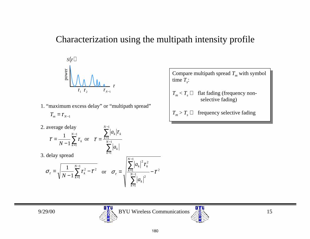
Characterization using the multipath intensity profile
( )τS
τ2τ1τ 1−Nτ
1. “maximum excess delay” or “multipath spread”
1−= NmT τ
∑−
=−=
1
11
1 N
kkN
ττ∑
∑−
=
−
== 1
1
1
1N
kk
N
kkk
a
a ττ
2. average delay
or
3. delay spread
21
1
2
1
1 ττστ −−
= ∑−
=
N
kkN
21
1
2
1
1
22
ττ
στ −=∑
∑−
=
−
=N
kk
N
kkk
a
aor
Compare multipath spread Tm with symboltime Ts:
Tm < Ts ⇒ flat fading (frequency non-selective fading)
Tm > Ts ⇒ frequency selective fading
Compare multipath spread Tm with symboltime Ts:
Tm < Ts ⇒ flat fading (frequency non-selective fading)
Tm > Ts ⇒ frequency selective fading
pow
er
180
9/29/00 BYU Wireless Communications 16
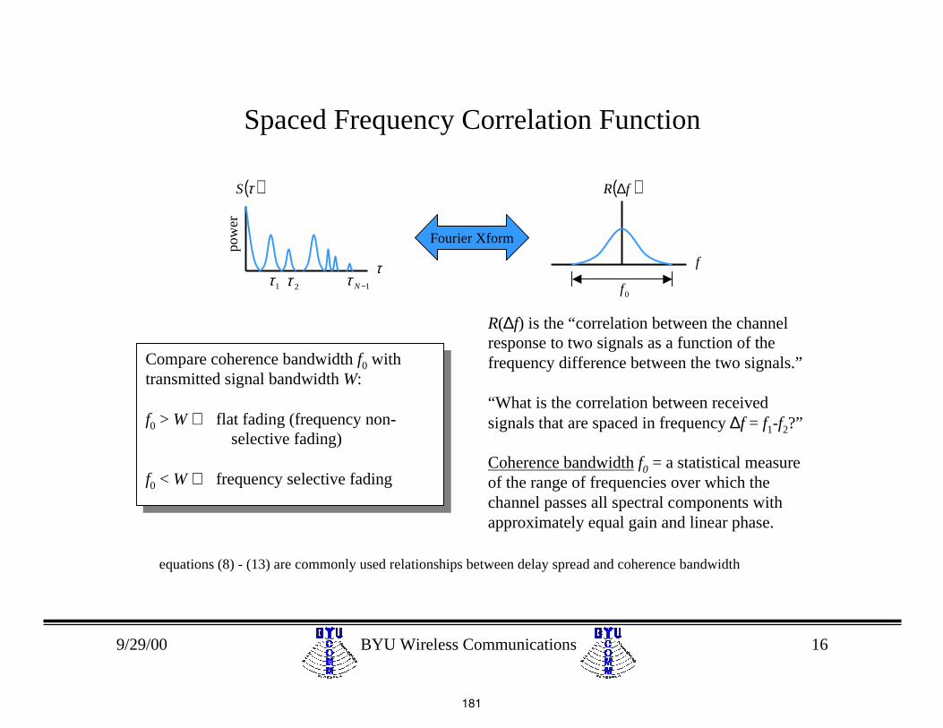
Spaced Frequency Correlation Function
( )τS
τ2τ1τ 1−Nτ
( )fR ∆
f
0f
Fourier Xformpo
wer
R(∆f) is the “correlation between the channelresponse to two signals as a function of thefrequency difference between the two signals.”
“What is the correlation between receivedsignals that are spaced in frequency ∆f = f1-f2?”
Coherence bandwidth f0 = a statistical measureof the range of frequencies over which thechannel passes all spectral components withapproximately equal gain and linear phase.
Compare coherence bandwidth f0 withtransmitted signal bandwidth W:
f0 > W ⇒ flat fading (frequency non-selective fading)
f0 < W ⇒ frequency selective fading
Compare coherence bandwidth f0 withtransmitted signal bandwidth W:
f0 > W ⇒ flat fading (frequency non-selective fading)
f0 < W ⇒ frequency selective fading
equations (8) - (13) are commonly used relationships between delay spread and coherence bandwidth
181

9/29/00 BYU Wireless Communications 17
Time Variations
Important Assumption
Multipath interference is spatial phenomenon. Spatial geometry is assumed fixed. Allscatterers making up the channel are stationary -- whenever motion ceases, the amplitude andphase of the receive signal remains constant (the channel appears to be time-invariant).Changes in multipath propagation occur due to changes in the spatial location x of thetransmitter and/or receiver. The faster the transmitter and/or receiver change spatial location,the faster the time variations in the multipath propagation properties.
( )
( ) ( )∑
∑−
=
−
=
−+=
−=
1
1
)(0
1
0
)(
)()()(
)()();(
N
kk
xjk
N
kk
xjk
xtexatxa
xtexaxth
k
k
τδδ
τδ
θ
θ
line-of-sightpropagation
multipathpropagation
complex gains andphase shifts are afunction of spatiallocation x.
182

9/29/00 BYU Wireless Communications 18
Spatially Varying Channel Impulse Response
τ
x
);( xth
• channel impulse response changeswith spatial location x
• generalize impulse response toinclude spatial information
• Transmitter/receiver motion causechange in spatial location x
• The larger , the faster the rate ofchange in the channel.
• Assuming a constant velocity v, theposition axis x could be changed to atime axis t using t = x/v.
);()( xthth →
x&
183
9/29/00 BYU Wireless Communications 19
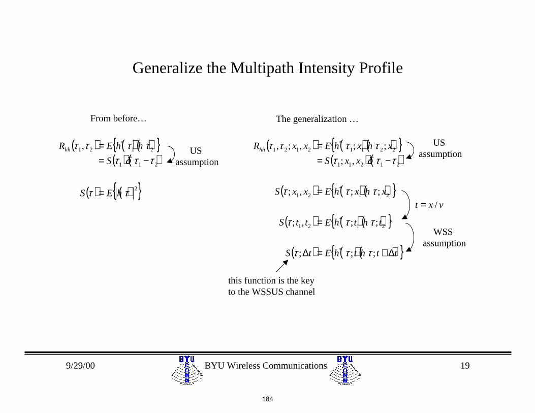
Generalize the Multipath Intensity Profile
( ) ( ) ( ){ }( ) ( )
( ) ( ){ }2
211
21*
21,
ττ
ττδτττττ
hES
S
hhERhh
=
−== ( ) ( ) ( ){ }
( ) ( )
( ) ( ) ( ){ }
( ) ( ) ( ){ }
( ) ( ) ( ){ }tththEtS
ththEttS
xhxhExxS
xxS
xhxhExxRhh
∆+=∆
=
=
−==
;;;
;;,;
;;,;
,;
;;,;,
*
21*
21
21*
21
21211
2211*
2121
τττ
τττ
τττ
ττδτττττ
From before… The generalization …
US assumption
US assumption
vxt /=
WSS assumption
this function is the keyto the WSSUS channel
184

9/29/00 BYU Wireless Communications 20
A look at S(τ;∆t)
τ
x∆
);( xS ∆τ
τ
t∆
);( tS ∆τ
( ) ( )0;ττ SS =
S(τ)S(τ)
185

9/29/00 BYU Wireless Communications 21
Time Variations of the Channel:The Spaced-Time Correlation Function
t∆
);( tS ∆τ
integrate along delay axis
t∆)( tR ∆
( ) ∫ ∆=∆ ττ dtStR );(
186

9/29/00 BYU Wireless Communications 22
Time Variations of the Channel:The Spaced-Time Correlation Function
0 0T t∆
)( tR ∆
R(∆t) specifies the extent to which there is correlation between the channelresponse to a sinusoid sent at time t and the response to a similar sinusoid attime t+∆t.
Coherence Time T0 is a measure of the expected time duration over whichthe channel response is essentially invariant. Slowly varying channels have alarge T0 and rapidly varying channels have a small T0.
187
9/29/00 BYU Wireless Communications 23
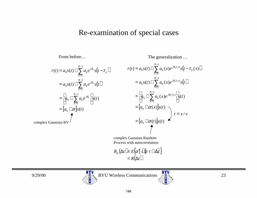
Re-examination of special cases
( )
( )
[ ] )(
)(
)(
)()(
0
1
10
1
10
1
10
tsa
tseaa
tseatsa
tseatsatr
N
k
jk
N
k
jk
N
kk
jk
k
k
k
α
τ
θ
θ
θ
+=
+=
+≈
−+=
∑
∑
∑
−
=
−
=
−
=
( )
( )
[ ]
[ ] )()(
)()(
)()(
)()(
)()()()(
0
0
1
1
)(0
1
1
)(0
1
1
)(0
tsta
tsxa
tsexaa
tsexatsa
xtsexatsatr
N
k
xjk
N
k
xjk
N
kk
xjk
k
k
k
α
α
τ
θ
θ
θ
+=
+=
+=
+≈
−+=
∑
∑
∑
−
=
−
=
−
=
complex Gaussian RV
vxt /=
complex Gaussian RandomProcess with autocorrelation
( ) ( ) ( ){ }( )tR
tttEtR
∆=∆+=∆ ααα
*
From before… The generalization …
188

9/29/00 BYU Wireless Communications 24
Commonly Used Spaced-Time Correlation Functions
( ) ∞<∆<∞−=∆ ttR a22σ
( ) tv
a etR∆−
=∆ λπ
σ2
22
( )
∆=∆ t
vJtR a λ
πσ 22 02
( )2
22
∆−
=∆t
v
a etR λπ
σ
( )t
v
tv
tR a
∆
∆
=∆
λπ
λπ
σ2
2sin2 2
Time Invariant
Land Mobile(Jakes)
Exponential
Gaussian
“Rectangular”
t∆
( )tR ∆
t∆
( )tR ∆
t∆
( )tR ∆
t∆
( )tR ∆
t∆
( )tR ∆
189

9/29/00 BYU Wireless Communications 25
Characterization of time variations using the spaced-timecorrelation function
0 0T t∆
)( tR ∆
• Fast Fading– T0 < Ts
– correlated channel behavior lasts less than a symbol ⇒ fading characteristicschange multiple times during a symbol ⇒ pulse shape distortion
• Slow Fading– T0 > Ts
– correlated channel behavior lasts more than a symbol ⇒ fading characteristicsconstant during a symbol ⇒ no pulse shape distortion ⇒ error bursts…
190
9/29/00 BYU Wireless Communications 26
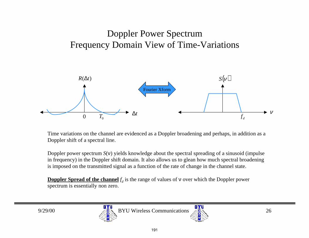
Doppler Power SpectrumFrequency Domain View of Time-Variations
0 0T t∆
)( tR ∆
Fourier Xform
( )νS
νdf
Time variations on the channel are evidenced as a Doppler broadening and perhaps, in addition as aDoppler shift of a spectral line.
Doppler power spectrum S(ν) yields knowledge about the spectral spreading of a sinusoid (impulsein frequency) in the Doppler shift domain. It also allows us to glean how much spectral broadeningis imposed on the transmitted signal as a function of the rate of change in the channel state.
Doppler Spread of the channel fd is the range of values of ν over which the Doppler powerspectrum is essentially non zero.
191

9/29/00 BYU Wireless Communications 27
Doppler Power Spectrum and Doppler Spread
( )νS
νdf
Compare Doppler Spread fd withtransmitted signal bandwidth W:
fd > W ⇒ fast fading
fd < W ⇒ slow fading
Compare Doppler Spread fd withtransmitted signal bandwidth W:
fd > W ⇒ fast fading
fd < W ⇒ slow fading
equations (18) - (21) are commonly used relationships between Doppler spread and coherence time
192

9/29/00 BYU Wireless Communications 28
Common Doppler Power Spectra
Time Invariant
Land Mobile(Jakes)
Exponential(1st order Butterworth)
Gaussian
“Rectangular”
ν
( )νS
( ) ( )νδσν 22 aS =
( )( )22
2
/
2
λνσν
vS a
−=
( ) ( )( )22
2
/
/2
λνπλσν
v
vS a
+=
( )( )
( )2
2
/
2
2
/
2 λν
λπσν va ev
S−
=
( )
<<−=otherwise0
///
2
λνλλ
σν vv
vSa
ν
( )νS
ν
( )νS
ν
( )νS
ν
( )νS
193

9/29/00 BYU Wireless Communications 29
Putting it all together…
( )fR ∆
f
0f
( )τS
τ2τ1τ 1−Nτ
pow
er
0 0T t∆
)( tR ∆
( )νS
νdf
);( tfS ∆∆
0=∆f0=∆t
Fourier transform Fourier transform
);( ντS
∫ νντ dS );( ∫ τντ dS );(
);( tS ∆τ Fourier transform
f∆↔τ
spaced-frequencycorrelation function
multipath intensityprofile
spaced-timecorrelation function
Doppler powerspectrum
spaced-frequency, spaced-time correlation function
scattering function
194
9/29/00 BYU Wireless Communications 30
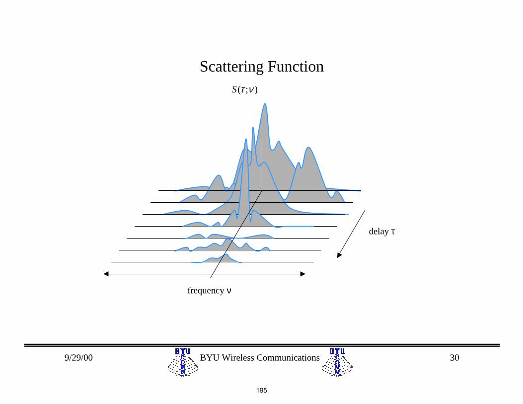
Scattering Function
delay τ
frequency ν
);( ντS
195

9/29/00 BYU Wireless Communications 31
References
• John Proakis, Digital Communications, Third Edition. McGraw-Hill. Chapter 10.
• William Jakes, Editor, Microwave Mobile Communications. John Wiley & Sons.Chapter 1.
• William Y. C. Lee, Mobile Cellular Communications, McGraw-Hill.
• Parsons, J. D., The Mobile Radio Propagation Channel, John Wiley & Sons.
• Bernard Sklar, “Rayleigh Fading Channels in Digital Communication systems Part I:Characterization,” IEEE Communication Magazine, July 1997, pp. 90 - 100.
• Peter Bello, “Characterization of Randomly Time Variant Linear Channels,” IEEETransactions on Communication Systems, vol. 11, no. 4, December 1963, pp. 360-393.
• R. H. Clarke, “A Statistical Theory of Mobile Radio Reception,” Bell Systems TechnicalJournal, vol. 47, no. 6, July-August 1968, pp. 957-1000.
• M. J. Gans, “A Power-Spectral Theory of Propagatio9in in the Mobile RadioEnvironment,” IEEE Transactions on Vehicular Technology, vol. VT 21, February1972, pp. 27-38.,
196


