MULTIPLE COMPARISON PROCEDURES IN FACTORIAL DESIGNS USING ...

MULTIPLE COMPARISON PROCEDURES IN FACTORIAL

DESIGNS USING THE ALIGNED RANK TRANSFORMATION

by

MARISELA ABUNDIS, B.S.

A THESIS

IN

STATISTICS

Submitted to die Graduate Faculty of Texas Tech University in

Partial Fulfillment of the Requirements for

the Degree of

MASTER OF SCIENCE

Approved

May, 2001

ACKNOWLEDGMENTS

First of all, I would like to thank my advisor, Dr. Mansouri for his help, support

and patience throughout my coursework and thesis. Thank you so much. Also. I

greatly appreciate the help I received from Dr. Westfall with some of my programming

required for the thesis. Dr. Duran, I thank you for your suggestions on my thesis and

answers to my questions. Thanks again to these outstanding professors.

Para mi familia, especialmente mis padres, agradezco mucho su apollo y comprension

durante todos los afios escolares de mi vida. Ustedes son la razon por la cual sigo

adelante. Los quiero mucho!

I would also like to thank my fiance, Jeffrey Martinez. Even though as undergrads

we went through very stressful and hard times, we managed to brighten each other

up and enjoy our college years. I love you!

Also, I greatly appreciate the friendship and love I have received from Jefirey's

parents. Thank you! To my best friend, Monet Alvarez, I thank you for always being

there for me since we were kids. I thank my other two closest friends, John Gomez

and Ina Aguirre. You two always keep my laughing!

I thank all the professors I have had at Texas Tech University, who have allowed

me to gain more mathematical and statistical skills. Thanks to Dr. Bennett, who

has always been a wonderful person to me, and without him I would not be here.

I would also like to thank my closest college friend, Ruby Martinez. I have always

enjoyed your company and will continue to do so as we proceed with our lives. Thanks

for j)utting up with me. I thank Richard Campos, Norma Aguirre, Bernard Omolo,

.Armando Arciniega, Carrie Mahood, and the custodians of the mathematics and

statistics department for being great friends to me.

11

CONTENTS

ACKNOWLEDGMENTS h

LIST OF TABLES iv

LIST OF FIGURES viii

I INTRODUCTION 1

II ANALYSIS OF VARIANCE AND MULTIPLE COMPARISON PROCE

DURES FOR A TWO-FACTOR FACTORIAL DESIGN 3

2.1 Analysis of Variance 3

2.2 Multiple Comparison Procedures 5

III ALIGNED RANK TRANSFORM TECHNIQUE 7

I\^ APPLICATIONS 11

4.1 A Balanced Two-Factor Factorial Design 11

4.2 Residual Analysis 15

4.3 An Unbalanced Two-Factor Factorial Design 25

V SIMULATIONS AND POWER STUDY 40

5.1 Simulations 41

5.2 Results 44

\T CONCLUSION 51

BIBLIOGRAPHY 52

111

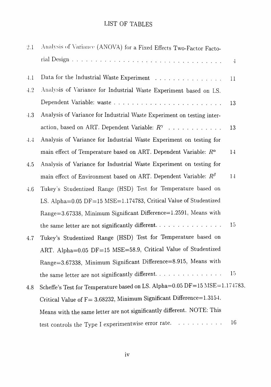
LIST OF TABLES

2.1 Analysis of Varianc(> (ANOVA) for a Fixed Effects Two-Factor Facto

rial Design 4

4.1 Data for the Industrial Waste Experiment U

4.2 Analysis of \ariance for Industrial Waste Experiment based on LS.

Dependent Variable: waste 13

4.3 Analysis of Variance for Industrial Waste Experiment on testing inter

action, based on ART. Dependent Variable: W 13

4.4 Analysis of Variance for Industrial Waste Experiment on testing for

main effect of Temperature based on ART. Dependent Variable: i?" 14

4.5 Analysis of Variance for Industrial Waste Experiment on testing for

main eflfect of Environment based on ART. Dependent Variable: R^ 14

4.6 Tukey's Studentized Range (HSD) Test for Temperature based on

LS. Alpha=0.05 DF=15 MSE=1.174783, Critical Value of Studentized

Range=3.67338, Minimum Significant Diflference= 1.2591, Means with

the same letter are not significantly diflferent 15

4.7 Tukey's Studentized Range (HSD) Test for Temperature based on

ART. Alpha=0.05 DF=15 MSE=58.9, Critical Value of Studentized

Range=3.67338, Minimum Significant Diflference=8.915, Means with


4.8 Scheffe's Test for Temperature based on LS. Alpha=0.05 DF=15 MSE=1.174783,

Critical Value of F= 3.68232, Minimum Significant Diflference=1.3154,

Means with the same letter are not significantly diflferent. NOTE: This

test controls the Type I experimentwise error rate 16

IV

4.9 Scheflfe's Test for Temperature based on .ART. .Alpha=0.05 DF=15

MSE=58.9. Critical \ alue of F=3.68232, Minimum Significant Diflfer-

ence=9.3143. Means with the same letter are not significantly different.

XOTE: This test controls the Type I experimentwise error rate. . . . 16

4.10 Tukey's Studentized Range (HSD) Test for Environment based on

LS. Alpha=0.05 DF-=15 MSE=1.174783, Critical \ alue of Studentized

Range=4.36699, Minimum Significant Difference=1.9323, Means with


4.11 Tukey's Studentized Range (HSD) Test for Environment based on

ART. Alpha=0.05 DF=15 MSE=61.83333. Critical \ alue of Studen

tized Range=4.36699, Minimum Significant Diflference=14.019. Means

with the same letter are not significantly diflferent 17

4.12 Scheflfe's Test for Environment based on LS. Alpha=0.05 DF=15 MSE=1.174783,

Critical \'alue of F=3.05557, Minimum Significant Difference=2.1877,

Means with the same letter are not significantly different. NOTE: This

test controls the Type I experimentwise error rate IS

4.13 Scheffes Test for Environment based on ART. Alpha=0.05 DF=15

MSE=61.83333, Critical \'alue of F=3.05557, Minimum Significant

Difference=15.872. Means with the same letter are not significantly

different. NOTE: This test controls the Type I experimentwise error

rate 18

4.14 Testing hypothesis at a = 0.05 significance level for both least squares

and ART methods/Industrial Waste Experiment 19

4.15 Multiple Comparison Procedures for both least squares and ART meth

ods/Industrial Waste Experiment 19

4.16 Analysis of Variance for testing equality of variances. Dependent \'ari-

able: Y 24

4.17 Drug Study Data 26

4.18 Drug Study Data (cell means for zj) 27

4.19 Analysis of Variance for Drug Study based on LS. Dependent X'ariable:

Y 28

4.20 Analysis of Variance for Drug Study on testing interaction, based on

ART. Dependent Variable: W 28

4.21 Analysis of Variance for Drug Study on testing for the main eflfect of

Drug, based on ART 29

4.22 Analysis of Variance for Drug Study on testing for the main eflfect of

Disease, based on ART. Dependent Variable: R^ 29

4.23 Least Squares Means for Eflfect drug Pr > \t\ for HO: LSMean(i)=LSMean(j)

Dependent Variable: Y based on LS, Adjustment for Multiple Com

parisons: Tukey 30


Dependent Variable: R^ based on ART, Adjustment for Multiple Com

parisons: Tukey 30



parisons: Scheflfe 31




VI

4.27 Least Squares Means for Effect drug Pr > \t\ for HO: LSMean(i)=LSMean(j)


parisons: Tukey 32

4.28 Least Squares Means for eflfect Disease Pr > |t| for HO: LSMean(i)=LSMean(j)


parisons: Tukey 32

4.29 Least Squares Means for eflfect Disease Pr > \t\ for HO: LSMean(i)=LSMean(j)



4.30 Least Squares Means for effect Disease Pr > \t\ for HO: LSMean(i)=LSMean(j)



4.31 Testing hypothesis at a = 0.05 significance level for both least squares

and ART methods/Drug Study 34

4.32 Multiple Comparison Procedures for both least squares and ART meth

ods/Drug Study 34

5.1 Design 1 43

5.2 Design 2 43

5.3 Design 3 43

5.4 Design 4 43

5.5 Design 5 43

5.6 Power simulation for all pairwise comparisons of Design 1 based on the

least squares and aligned rank transform methods 47



Vll







5.11 Power simulation for all pairwise comparisons of Table 4.1, Data for

Industrial Waste Output based on the least squares and aligned rank

transform methods 49

5.12 Power simulation for all pairwise comparisons of Table 4.5, Drug Study

Data based on the least squares and aligned rank transform methods 50

viu

LIST OF FIGURES

4.1 Residuals versus YEAR 20

4.2 Residuals versus Temperature 21

4.3 Residuals versus Environment 22

4.4 Normal Probability Plot 23

4.5 Residuals versus YEAR 35

4.6 Residuals versus Drug 35

4.7 Residuals versus Disease 37

4.8 Normal Probability Plot 38

IX

CHAPTER I

INTRODUCTION

A factorial design is used for an experiment that involves the study of two or more

factors simultaneously, with each factor having two or more levels. The importance

of factorial designs is that they permit simultaneous examination of the effects of

individual factors and their interactions. All possible combinations of the levels of

the factors are investigated in each replication of an experiment. .A main effect is

defined as the change in response produced by a change in the level of one factor

while keeping the remaining factors at a fixed level. Interaction exists between two

factors if the difference in response between the levels of one factor is not the same

at all levels of the other factors. Thus, the preliminary focus of analysis is testing

hypotheses about interaction, equality of row treatment effects, and column treatment

eflfects. If interaction exists, main effects exists as well. If interaction does not exist.

then testing main effects should proceed. In Chapter II, we present the analysis of

variance for a two-factor factorial fixed effects factorial design.

The hypotheses do not provide detailed information about the difference in inter

actions and main eflfects. Multiple comparison procedures are capable of responding

to specific questions about more meaningful comparisons on any of the above eflfects.

These procedures allow the comparisons between groups or pairs of treatment means.

The comparisons are made in terms of treatment totals or treatment averages. It

must be noted that multiple comparison techniques are not dependent on the re

jection of null hypothesis. The testing of interaction between two factors and main

eflfects can also be performed by multiple comparison methods. Common multiple

comparison procedures that will be implemented are Tukey's Studentized Range T( st

and Scheflfe's Method. These multiple comparison procedures are discussed in Chap

ter II. Additionally, we will employ a macro called %SimPower in order to perform

multiple comparisons. This macro was developed by Tobias (see Westfall et al.. 1999).

%SimPower simulates power for multiple comparisons. It uses complete, mini

mal, and proportional power definitions. Complete power is defined as the probability

of rejecting all false null hypotheses. Minimal power is the probability that at least

one false null hypothesis is rejected implying a significant result. Proportional power

is the proportion of false null hypotheses detected to all false null hypotheses, that is

false nulls expected to be detected. Further discussion is provided in Chapter \ ' .

One of the main purposes of this investigation is to carry out multiple comparisons

for twô-factor factorial designs based on the aligned rank transformation. The aligned

rank transform procedure provides a robust and powerful alternative method of data

analysis to the classical least squares method. In this investigation, we will study the

validity and power of the aligned rank transform technique for multiple comparisons.

In Chapter III, we define the classical least squares F-statistic and the aligned rank

transform technique.

Analysis of two applications based on the least squares and aligned rank transform

methods will be examined in Chapter IV. The final conclusion will be provided in

Chapter VI. We will utilize the SAS programming language to perform the classical

least squares method and the aligned rank transform technique. P R O C GLM,

PROG REG, and P R O C R A N K will execute the two techniques. These ideas

will be explained in more detail later on.

CHAPTER II

ANALYSIS OF VARIANCE AND MULTIPLE COMPARISON PROCEDURES

FOR A TWO-FACTOR FACTORIAL DESIGN

In this chapter, we present the analysis of variance and multiple comparison pro-

cefures for a fixed effects two-factor factorial design.

2.1 Analysis of Variance

Suppose that an experiment involves the simultaneous study of two factors A and

B. Let yijk denote the k-th replication in response under the i-th level of factor A and

j-th level of factor B. It is assumed that yijk follows the linear model

Vijk = Id + ai -\- Pj -\- {al3)ij + Cijk,

i=l,...,a

j=l,...,b

k=l,...,n

(2.1)

where,

a is the number of levels of factor A,

b is the number of levels of factor B,

n is the number of replications,

// is the overall mean,

a, is the main eflfect of the (ith) level of factor A,

Pj is the main eflfect of the (jth) level of factor B,

{aP)ij is the interaction between the i-th level of factor A and j-th level of factor B,

and Cijk are the random error components.

The linear model has the following restrictions:

EU ^^ = 0

Table 2.1: Analysis of Variance (ANOVA) for a Fixed Effects Two-Factor Factorial Design

Source of Variation

Sum of Squares

Degrees of Freedom

Mean Squares Fa

A

B

AB

Error

Total

SSA

SS B

SS AB

SSt

SSi

a- 1

6 - 1

( a - l ) ( 6 - l )

ab(n — 1)

abn — 1

SSA MSA = ^

^ a—I

MSB = I^

A f c _ SSAB IMbAB - ( a - l ) ( 6 - l )

MSE - ^^^ ab{n—l)

MSA

MSE

MSB

MSE

-U5.45

MSE

It is assumed that eij are independent and indentically distributed random variables

with ^"(0,^^) distribution, where N{/j,,a'^) denotes a normal distribution with mean

Ij, and variance cr .

The quantities in the table are presented as:

SSA - TZ Jliî y y:.. abn

abn

hj. yl abn

abn

SSB - j5 E ; = i ytj. -

SS.B = i EU EU Vl - £ - SSA - SS

SSs = SSr-i; EU EU y

SST = zJi=l l^j = l Z A:=1 Vijk

where,

E a \~^^ v"^" i = l 2 . ^ j= l Z^k^l Vij^

i*"" abn

E n k-i y^ji^

y^J- ~ n

E a ^r-^n i= l 2^k=l yijii

y.j.

B

y.j. an

4

(2.2)

(2.3)

(2.4)

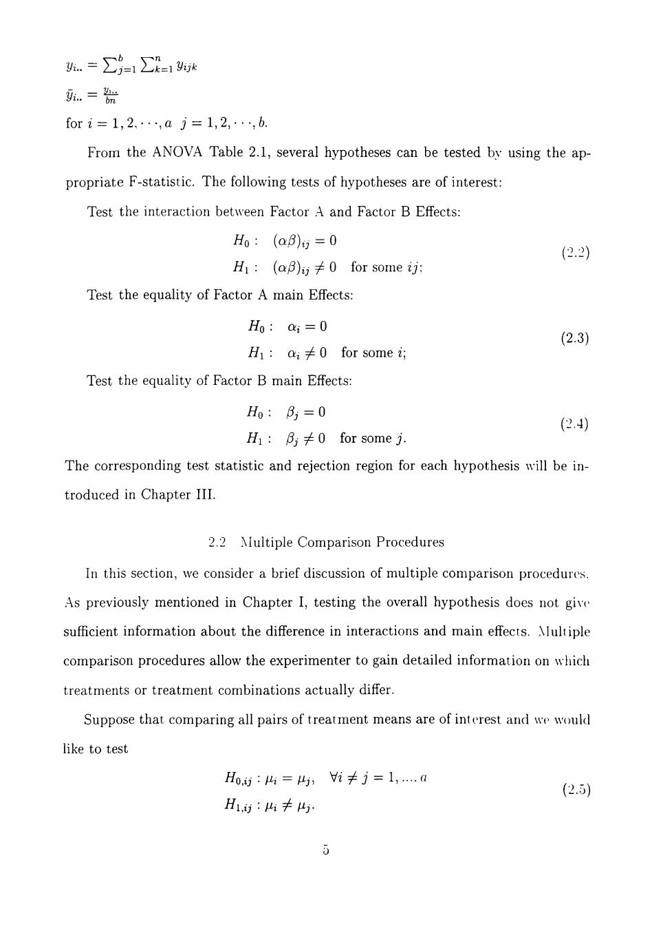
yi.. — /^j=i z^k=\ y^ji^

yi.. fjj^

for i := 1,2, • • -,0 j = 1,2, • • -,6.

From the ANOVA Table 2.1, several hypotheses can be tested by using the ap

propriate F-statistic. The following tests of hypotheses are of interest:

Test the interaction between Factor .A and Factor B Effects:

Ho: (a/3),, = 0

Hi : (oi.p)ij ^ 0 for some ij:

Test the equality of Factor A main Eflfects:

HQ : Off = 0

Hi : tti 7 0 for some i\

Test the equality of Factor B main Effects:

Ho: ft = 0

Hi : Pj ^ 0 for some j .

The corresponding test statistic and rejection region for each hypothesis will be in

troduced in Chapter HI.

2.2 Multiple Comparison Procedures

In this section, we consider a brief discussion of multiple comparison procedures.

As previously mentioned in Chapter I, testing the overall hypothesis does not give

sufficient information about the difference in interactions and main effects. Multiple

comparison procedures allow the experimenter to gain detailed information on which

treatments or treatment combinations actually diflfer.

Suppose that comparing all pairs of treatment means are of interest and wv would

like to test

Ho,ij : iit = Pj, \fiy^j = l,....a (2.0)

Hi,ij : Hi / Pj.

0

For our purposes, Tukey's studentized range statistic is used tu test the above

hypotheses. On experimentwise premise, Tukey's test has a family-wise Type I error

rate of a for all pairwise comparisons (see Montgomery, 1997). It strongly controls

the family-wise Type I error rate and is the most powerful for pairwise comparison.

Rejection of 7/o,ij results if |^j. — yj.\ > Ta = ^0(0, f)Sy^,, where qa{a, f) is the upper

a percentage point of the studentized range for groups of means, Sy^ = v/^^^^ is the

standard error of each average, a is the number of means in a group, / is the degrees

of freedom for error.

If the comparison involves more than two means, then Scheffe's test is the best

method for such comparisons. Scheflfe's test compares any and all contrasts between

means. .A contrast is a linear combination of treatment totals. That is, C = Yll^=i îVf

with the constraint J2^=iî — 0- - 0 is rejected if \Cu\ > Sa,u' where C^ is any

possible linear combination of interest and Sa,u = Sc^ \J{a — l)Faâ-i,iv-a< where

Scy, = SJMSE miLi(Qu^/î)- The Type I error is at most a for all possible compar

isons. Scheffe's test could also be applied to pairwise comparisons of means, though

it is not the most sensitive technique.

Tukey's and Scheffe's test are applied to the applications in Chapter I\', while in

simulation studies of Chapter V, we only apply Tukey's test.

6

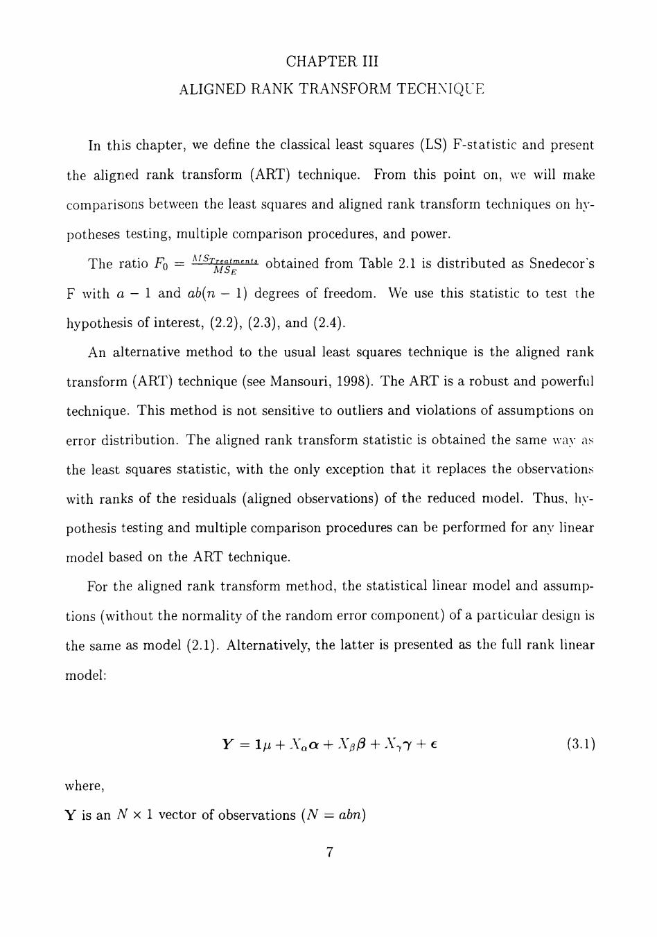
CHAPTER III

ALIGNED RANK TRANSFORM TECHNIQUE

In this chapter, we define the classical least squares (LS) F-statistic and present

the aligned rank transform (ART) technique. From this point on, we will make

comparisons between the least squares and aligned rank transform techniques on hy

potheses testing, multiple comparison procedures, and power.

The ratio FQ = '^^^Tr.a^tment, obtained from Table 2.1 is distributed as Snedecor's

F with a - I and ab{n - 1) degrees of freedom. We use this statistic to test the

hypothesis of interest, (2.2), (2.3), and (2.4).

An alternative method to the usual least squares technique is the aligned rank

transform (ART) technique (see Mansouri, 1998). The ART is a robust and powerful

technique. This method is not sensitive to outliers and violations of assumptions on

error distribution. The aligned rank transform statistic is obtained the same way as

the least squares statistic, with the only exception that it replaces the observations

with ranks of the residuals (aligned observations) of the reduced model. Thus, hy

pothesis testing and multiple comparison procedures can be performed for any linear

model based on the ART technique.

For the aligned rank transform method, the statistical linear model and assump

tions (without the normality of the random error component) of a particular design is

the same as model (2.1). Alternatively, the latter is presented as the full rank linear

model:

y = 1/i + Xâ -f Xp^ + X^j + € (3.1)

where,

Y is an TV X 1 vector of observations {N = abn)

7

1 is an A X 1 vector of ones

p is the y-intercept

cx= (ai, ...,aa-i)'

^=(Pu...jb-iy

7 = (7ll, •••,7l,6-l,-",7a-l,l'---'7a-l,6-l)'

e is an A X 1 vector of independent random variables with a continuous, unknown

distribution function

A'Q, Xp, X-y are full rank matrices with -1,0,1 entries, according to the specific design.

A reduced model is a linear model that includes all the unknown parameters except

the parameter of interest which is held constant. That is when the null hypothesis

(HQ) holds, then the reduced model is obtained.

The ART technique is developed in the following manner:

1. Fit the reduced model and obtain the corresponding residuals.

2. Rank the residuals.

3. Fit the reduced and the full models to the ranks.

The ART test statistic is:

J, ^[SSEreMR)]-SSEfMa{R)] ^"^ qMSEfuiila(R)] ^ ^^

where,

SSEreMR)] = «'(^)(^ - Hi)a(R)

SSEfûHR)] = a'(R){I - H)a(R)

MSEfûHR)] = {N- P)-'SSEfuu[a{R)]

P is the rank of H

q is the rank of H — Hi

[a{R)] is the vector of rank scores

Hi=Xi{X[Xi)-'^X[

H = X{X'X)-'^X'.

Hi and H are the respective hat matrices for the reduced and full models.

8

We now specify the corresponding test statistics and rejection regions for hypothe

ses (2.2), (2.3) and (2.4) based on both the classical least squares technique and the

aligned rank transform. Let T.S and R.R denote the test statistic and rejection re

gion for the classical least squares method, and T.SART and R.RART denote the

test statistic and rejection region for the ART method.

Referring to null and alternative hypotheses mentioned previously, we test the

following at a particular significance level (a):

Interaction between factor A and B effects:

^ c . P — MSA*B

T Q A R T • r ^ — MSRC[a{R-^)] l .O / \ rLl . r ^ ^ — MSElaiR-^)]

R . R : Fo > FaXa-\){b-\),ab{n-l)

R . R A R T : F ^ ^ > Faîâ-\){b-\),ab{n-\)

Main effect of factor A:

T Q • ;r — ^SA

T Q A R T • /?« - ^SR[a{R'^) i . D / \ n i . Fj^j^ — f^sE[a{R^)]

R . R : FQ > Fa,{a-l),ab{n-l)

R . R A R T : F J ^ > FaXa-\),ab{n-l)

Main effect of factor B:

T c; . F — ^SB

T Q A R T • F ^ - ^SC[a{R^)

(3.3)

(3.4)

(3 .5 )

R . R : FQ > Fa,{b-l),ab{n-l)

R . R A R T : F ^ ^ > Fa,(b-\),ab{n-l)

The following SAS program for the analysis of a two-way layout based on the .ART

method is given in Mansouri (1998):

data new; /*create a data set*/ do A = ai to Gr] /*A has r levels, B has c levels and rep has n replications*/ do B = bi to br] do rep = 1 to n; input Y@@;

9

output; end; end; end; datalines; data two way; set new;

/*define A^V if ,4 = "ai" then Xî = 1; if ^ = "a^" then Xî = - 1 ; else A' i = 0:...if -4 = "ar-i" then Xar-i = f; if ^ = "flr" then A^r-i = — 1; else X^r-i — 0;

/*define A>*/ if B = "6i" then Xpi = l;\iB = "6c" then A>i = - 1 ; else Xî = 0;...if B = "'6^-1'' then A/3C-1 = 1; ii B = ''be" then A^c-i = —^] else Xpc-i = 0;

/*define A / / A'-yii = A ' Q I A / 3 i ; . . . X ^ r - l , c - l = - ^ a r - l ^ / S c - l J

/*ART test statistic for testing i/o"*/ proc reg data=twoway; model Y = Xpi - A^c-1^711 ~ -^7r-i,c-i; output out=aligna r = K"; proc rank data=aligna out==rankya; ranks R°'; var V"; proc glm data=rankya; classes .A B; model R^=A B A*B; Ismeans A/lsd tukey scheffe;

/*ART test statistic for testing HQ^*/ proc reg data=twoway; model Y = A^ i ~ ^Qr-1^711 ~ ^7r-i,c-i; output out=alignb r = Y^\ proc rank data=alignb out=rankyb; ranks R^\ var Y^] proc glm data=rankyb; classes A B; model R^=A B A*B; Ismeans B/lsd tukey scheflfe;

/*ART test statistic for testing i/o^*/ proc reg data=twoway; model Y = AQI - Xar-iXpi — Xpc-i] output out=aligng r = Y^; proc rank data=aligng out=rankyg; ranks R^; var Y'^; proc glm data=rankyg; classes A B; model R'^=A B A*B;

10

CHAPTER IV

APPLICATIONS

In this chapter, the least squares and the ART method are applied to data sets

resulting from factorial experiments. The main objective is to show that the ART

procedure provides valid results for multiple comparisons and should be considered

as a feasible alternative to the procedures based on the least squares. We present

two types of designs, a balanced and an unbalanced two-factor factorial design. All

procedures are performed on SAS and the results are analyzed.

4.1 A Balanced Two-Factor Factorial Design

Industrial Waste Experiment: To remain competitive, businesses have adopted

a philosophy of continuous improvement of their manufacturing and service processes.

An important element of this philosophy is experimentation, to better understand

systems and to optimize performance. The data in the following study are from

an experiment designed to study the eflfect of temperature (at low. medium, and

high levels) and environment (five different enivornments) on waste ouput in a man

ufacturing plant (see Table 4.1). Two replicate measurements are taken at each

temperature/environment combination (Westfall et al., 1999, pp. 176 e 178).

Table 4.1: Data for the Industrial Waste Experiment

Temperature Low (1)

Medium (2)

High (3)

1 7.09 5.90 7.01 5.82 7.78 7.73

Environment 2

7.94 9.15 6.18 7.19 10.39 8.78

3 9.23 9.85 7.86 6.33 9.27 8.90

4 5.43 7.73 8.49 8.67 12.17 10.95

5 9.43 6.90 9.62 9.07 13.07 9.76

11

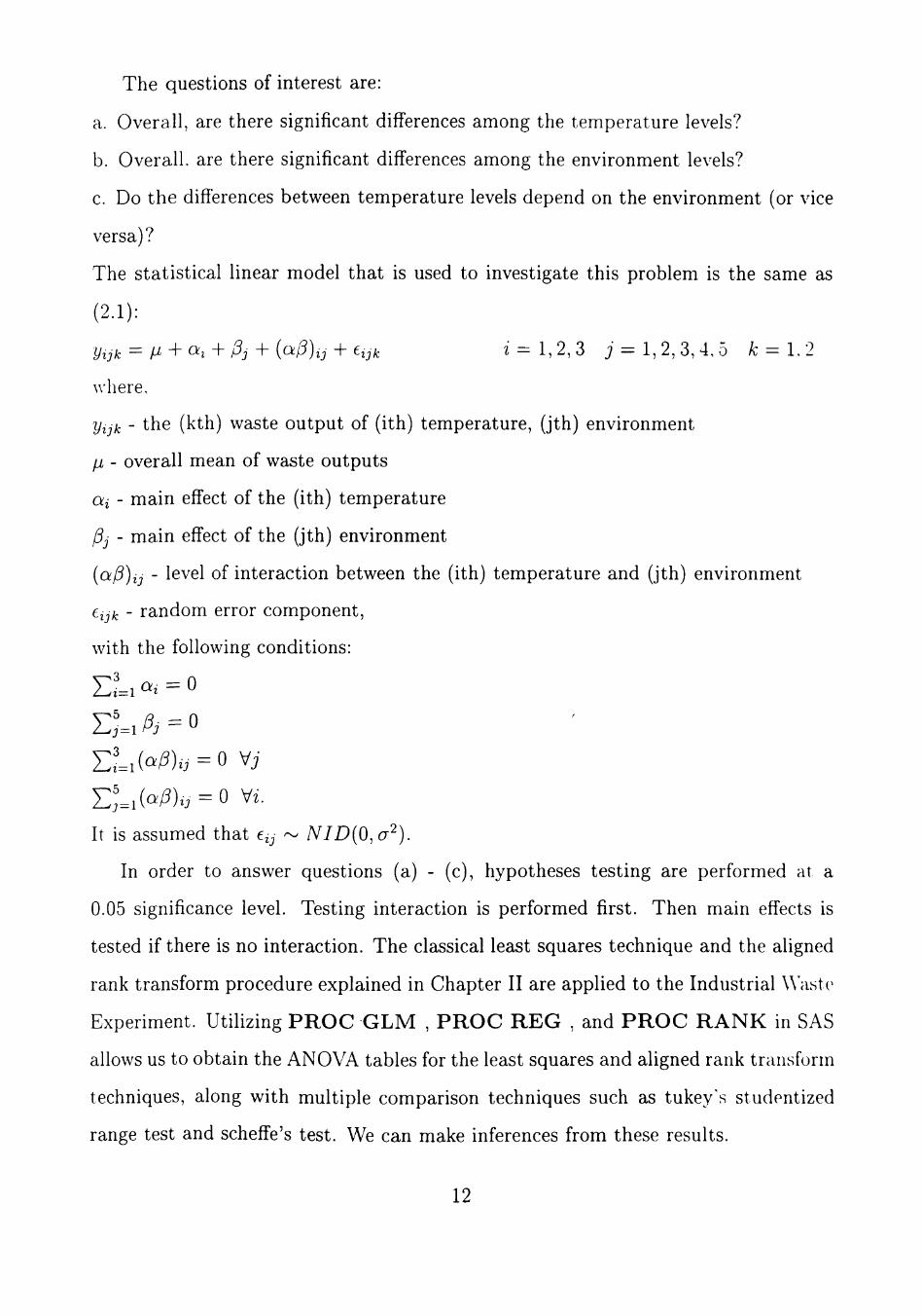
The questions of interest are:

a. Overall, are there significant differences among the temperature levels?

b. Overall, are there significant differences among the environment levels?

c. Do the differences between temperature levels depend on the environment (or vice

versa)?

The statistical linear model that is used to investigate this problem is the same as

(2.1):

yijk = P +(^1 +Pj-^ {c^(^)ij-Ûjk 2 = 1,2,3 7 = 1,2,3,4,5 k = 1.2

where,

y^jk - the (kth) waste output of (ith) temperature, (jth) environment

p - overall mean of waste outputs

ai - main effect of the (ith) temperature

13j - main effect of the (jth) environment

(Q^P)ij - level of interaction between the (ith) temperature and (jth) environment

Eijk - random error component,

with the following conditions:

E l l « . = 0

EU ft = 0

It is assumed that e,, ~ NID{0,a^).

In order to answer questions (a) - (c), hypotheses testing are performed at a

0.05 significance level. Testing interaction is performed first. Then main effects is

tested if there is no interaction. The classical least squares technique and the aligned

rank transform procedure explained in Chapter II are applied to the Industrial Waste

Experiment. Utilizing P R O C GLM , P R O C R E G , and P R O C R A N K in SAS

allows us to obtain the ANOVA tables for the least squares and aligned rank transform

techniques, along with multiple comparison techniques such as tukey's studentized

range test and scheffe's test. We can make inferences from these results.

12

Table 4.2: Analysis of Variance for Industrial Waste Experiment based on LS. Dependent Variable: waste

F Value Pr > F Source Model Error Corrected Total

Source envir*temp temp

DF 14 15 29

DF 8 2

Sum of Squares 78.28974667 17.62175000 95.91149667

Type I SS 22.91156000 30.69280667

Mean Square 5.59212476 1.17478333

Mean Square 2.86394500 15.34640333

4.76 0.0024

envir

F Value Pr > F 2.44 0.0651 13.06 0.0005

4 24.68538000 6.17134500 5.25 0.0075

Table 4.3: Analysis of Variance for Industrial Waste Experiment on testing interaction, based on ART. Dependent Variable: R^

Source Model Error Corrected Total

Source Temp Envir Temp*Envir

DF 14 15 29

DF 2 4 8

Sum of Squares 1295.000000 952.500000 2247.500000

Type I SS 12.800000 13.000000 1269.200000

Mean Square 92.500000 63.500000

Mean Square 6.400000 3.250000 158.650000

F Value 1.46

F Value 0.10 0.05 2.50

Pr > F 0.2391

Pr > F 0.9047 0.9945 0.0602

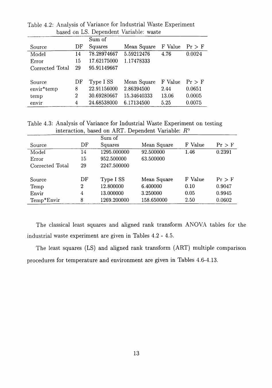
The classical least squares and aligned rank transform ANOVA tables for the

industrial waste experiment are given in Tables 4.2 - 4.5.

The least squares (LS) and aligned rank transform (ART) multiple comparison

procedures for temperature and environment are given in Tables 4.6-4.13.

13

Table 4.4: Analysis of Variance for Industrial Waste Experiment on testing for main eflfect of Temperature based on ART. Dependent \'ariable: R^


Source Temp Envir Temp* Envir

DF 14 15 29

DF 2 4 8

Sum of Squares 1364.000000 883.500000 2247.500000

Type I SS 1349.600000 4.000000 10.400000

Mean Square 97.428571 58.900000

Mean Square 674.800000 1.000000 1.300000

F Value 1.65

F Value 11.46 0.02 0.02

Pr > F 0.1723

Pr > F 0.0010 0.9994 1.0000

Table 4.5: Analysis of Variance for Industrial Waste Experiment on testing for main effect of Environment based on ART. Dependent Variable: R^^


Source Temp Envir Temp*Envir

DF 14 15 29

DF 2 4 8

Sum of Squares 1320.000000 927.500000 2247.500000

Type I SS 15.000000 1285.333333 19.666667

Mean Square 94.285714 61.833333

Mean Square 7.500000 321.333333 2.458333

F Value 1.52

F Value 0.12 5.20 0.04

Pr > F 0.2135

Pr > F 0.8866 0.0079 1.0000

Table 4.14 and Table 4.15 summarize the results from the conducted analysis. Let

us define the following abbreviations as:

LS is the the value of the least squares test statistic,

ART is the value of the aligned rank transform test statistic,

CV is the critical value used to determine if HQ is rejected or not,

P-VAL-LS is the smallest level of significance at which HQ can be rejected for the

usual least squares method,

P-VAL-ART is the smallest level of significance at which HQ can be rejected for the

aligned rank transform method,

{ti,tj) denotes temperature i as significantly different from temperature j .

14

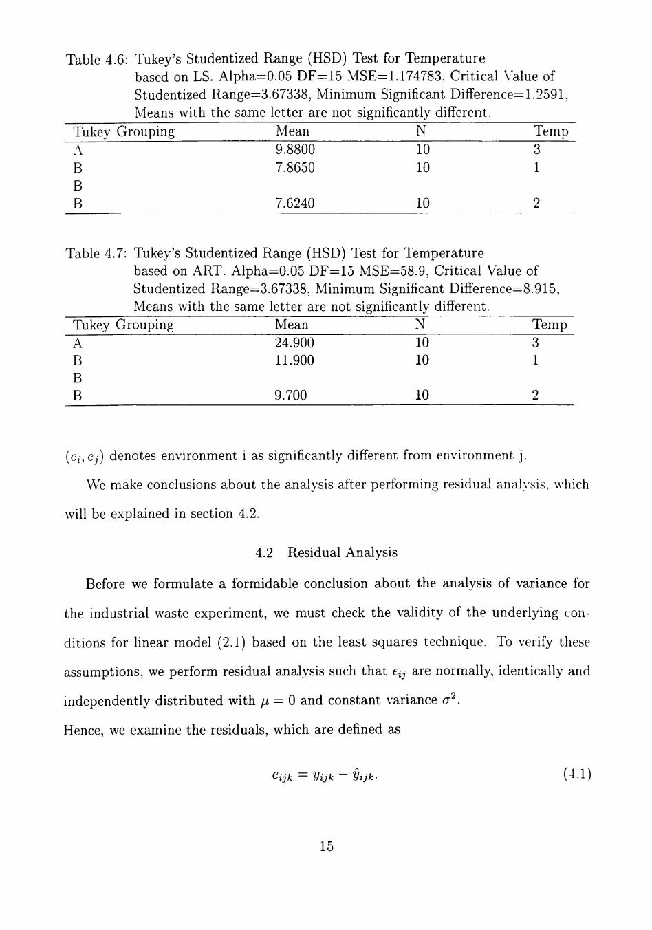
Table 4.6: Tukey's Studentized Range (HSD) Test for Temperature based on LS. Alpha=0.05 DF=15 MSE=1.174783, Critical Value of Studentized Range=3.67338, Minimum Significant Difference=1.2591, Means with the same letter are not significantly different.

Tukey Grouping A B B B

Mean 9.8800 7.8650

7.6240

N 10 10

10

Temp 3 1

2

Table 4.7: Tukey's Studentized Range (HSD) Test for Temperature based on ART. Alpha=0.05 DF=15 MSE=58.9, Critical Value of Studentized Range=3.67338, Minimum Significant Difference=8.915, Means with the same letter are not significantly different.

Tukey Grouping A B B B

Mean 24.900 11.900

9.700

N 10 10

10

Temp 3 1

2

(ej,ej) denotes environment i as significantly different from environment j .

We make conclusions about the analysis after performing residual analysis, which

will be explained in section 4.2.

4.2 Residual Analysis

Before we formulate a formidable conclusion about the analysis of variance for

the industrial waste experiment, we must check the validity of the underlying con

ditions for linear model (2.1) based on the least squares technique. To verify these

assumptions, we perform residual analysis such that Cij are normally, identically and

independently distributed with p = 0 and constant variance cr .

Hence, we examine the residuals, which are defined as

eijk = yijk - yijk^ (44)

15

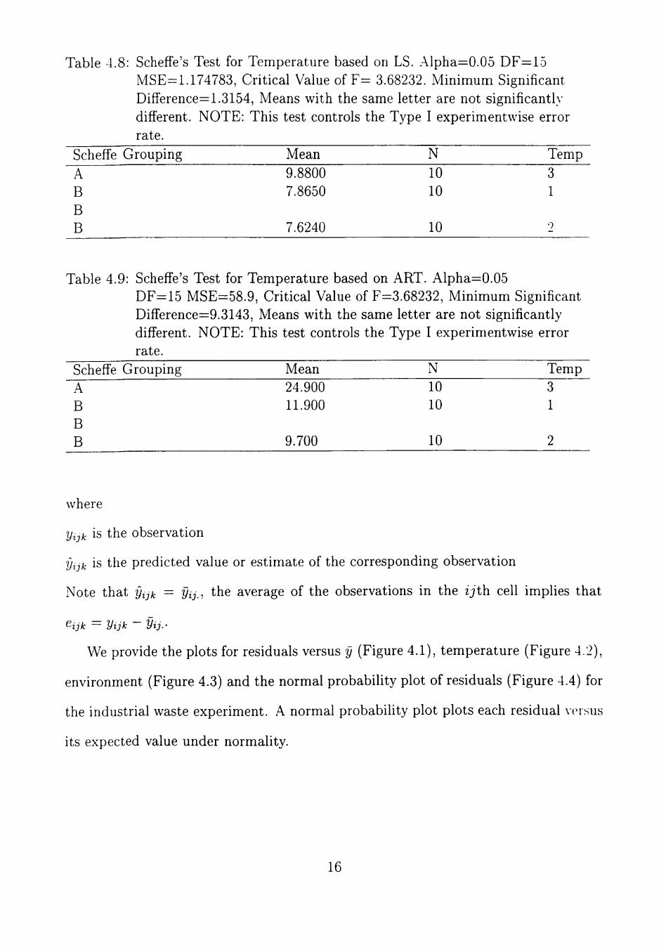
Table 4.8: Scheflfe's Test for Temperature based on LS. Alpha=0.05 DF=15 MSE=1.174783, Critical Value of F= 3.68232. Minimum Significant Difference=1.3154, Means with the same letter are not significantly different. NOTE: This test controls the Type I experimentwise error rate.

Scheffe Grouping Mean N Temp ~7. 9.8800 To 3

B 7.8650 10 1 B B 7.6240 10 2

Table 4.9: Scheflfe's Test for Temperature based on ART. Alpha=0.05 DF=15 MSE=58.9, Critical Value of F=3.68232, Minimum Significant Diflference=9.3143, Means with the same letter are not significantly different. NOTE: This test controls the Type I experimentwise error rate.

Scheflfe Grouping Mean N Temp ~A~ 24.900 To 3

B 11.900 10 1 B B 9.700 10 2

where

yiji^ is the observation

y^jk is the predicted value or estimate of the corresponding observation

Note that yijk = yij., the average of the observations in the ijth. cell implies that

îjk ^^ yijk ~ yij.-

We provide the plots for residuals versus y (Figure 4.1), temperature (Figure 4.2),

environment (Figure 4.3) and the normal probability plot of residuals (Figure 4.4) for

the industrial waste experiment. A normal probability plot plots each residual versus

its expected value under normality.

16

A A A A A A A

9.6417

8.9067

8.5733

8.2717

6.8883

6

6

6

6

6

Table 4.10: TUKEY'S STUDENTIZED RANGE (HSD) TEST for Environment based on LS. Alpha=0.05 DF=15 MSE=1.174783, Critical \ alue of Studentized Range=4.36699, Minimum Significant Difference=1.9323, Means with the same letter are not significantly diflferent.

Tukey Grouping Mean N Envir 5

4

B A 8.5733 6 3 B B A 8.2717 6 2 B B 6.8883 6 1

Table 4.11: Tukey's Studentized Range (HSD) Test for Environment based on ART. Alpha=0.05 DF=15 MSE=61.83333, Critical Value of Studentized Range=4.36699, Minimum Significant Difference=14.019, Means with the same letter are not significantly diflferent.

Tukey Grouping Mean N Envir T

4 A

B A 17.000 6 3 B B B B

A A A A A A A

23.000

19.667

17.000

14.000

3.833

6

6

6

6

6

Table 4.12: Scheffe's Test for Environment based on LS. Alpha=0.05 DF=15 MSE=1.174783, Critical Value of F=3.05557, Minimum Significant Difference=2.1877, Means with the same letter are not significantly diflferent. NOTE: This test controls the Type I experimentwdse error rate.

Scheflfe Grouping Mean N Envir A 9.6417 6 5 A

B A 8.9067 6 4 B A B A 8.5733 6 3 B A B A 8.2717 6 2 B B 6.8883 6 1

Table 4.13: Scheflfe's Test for Environment based on ART. Alpha=0.05 DF=15 MSE=61.83333, Critical Value of F=3.05557, Minimum Significant Diflference=15.872, Means with the same letter are not significantly different. NOTE: This test controls the Type I experimentwise error rate.

Scheflfe Grouping Mean N Envir

5

4

3

2

A A A A A A A

23.000

19.667

17.000

14.000

3.833

6

6

6

6

6

B B B B B B B 3.833 6 1

18

Table 4.14: Testing hypothesis at a = 0.05 significance level for both least squares and ART methods/Industrial Waste Experiment

EFFECTS Interaction

Temp. Environ.

LS 2.44 13.05 5.25

ART 2.50 11.46 5.20

CV 2.64 3.68 3.06

P-VAL-LS 0.0651 0.0005 0.0075

P-VAL-ART 0.0602 0.0010 0.0079

Table 4.15: Multiple Comparison Procedures for both least squares and ART methods/Industrial Waste Experiment

EFFECTS Temp. (1,2,3)

Environ. (1,2,3,4,5)

Tukey-LS ( ^ 3 , ^ l )

(^3,^2)

( 6 5 , 6 1 )

( 6 4 , 6 1 )

Tukey-ART (^3,^1)

(^3,^2)

( 6 5 , 6 1 )

( 6 4 , 6 1 )

Scheflfe-LS (^3,^1)

(^3,^2)

( 6 5 , 6 1 )

Scheflfe-ART (^3 ,^1)

(^3 ,^2)

( 6 5 , 6 1 )

19

ybar

Figure 4.1: Residuals versus YBAR

20

2 . 5

2 . 0 -

O

1 . 5

O

o

Temperature

Figure 4.2: Residuals versus Temperature

21

Environment

Figure 4.3: Residuals versus Environment

22

i 1 /

/ /

/ /

/ /

9 /

/ /

G /

/

o

o /

/ o^

o

/ / o

o GJ'OO /

O / o/

/

e

- 2 i / /

/

/ /

/ 1/ - 3 —I 1 1 1 1 r

3 - 2 - 1 0 1 2 3

N o r m a l Q u a n t i l e s

N o r m a l L i n e : — Mu=0, S i g m a = l

Figure 4.4: Normal Probability Plot

23

Table 4.16: .Analysis of Variance for testing equality of variances. Dependent Variable: Y

Sum of Source DF Squares Mean Square F \'alue Pr > F

Model 4 3.68815333 0.92203833 0.70 0.5986 Error 25 32.88431667 1.31537267 Corrected Total 29 36.57247000

Source DF Type I SS Mean Square F \'alue Pr > F environment 4 3.68815333 0.92203833 0.70 0.5986

From Figures 4.1 and 4.2, we observe that the plots do not contain outliers. \\V

note that Figure 4.3 clearly shows a trumpet-like pattern, implying that the error

variance is not constant for different environments. We can further investigate or

reexamine the data from the study of regression analysis. Let us perform the modified

Levene's test. Levene's test conducts a test for equality of variances in all treatments

(environment) at a 0.05 significance level. The modified Levene test (see Montgomery,

1997) calculates the absolute deviation of observations yijk in each treatment from the

treatment median {yjk)- Similarly the previous is denoted as dijk = \yijk-yjk\^ where

2 = 1,2,3 j = 1,2,3,4,5 k = 1,2. The test statistic is the classical F-statistic,

used in Table 4.14. Let us provide the reader with the corresponding ANOVA Table

4.16.

From the ANOVA table, we obtain a p-value=0.5986 greater than the 0.05 signif

icance level, thus implying that we do not reject HQ. That is, variances are constant,

hence satisfying the assumption. We observe from the normal probability plot (Fig

ure 4.4) that a straight line is represented by the residuals, implying that the errors

are normally distributed.

We can now answer questions (a) - (c). From Table 4.14, we observe that the least

squares and aligned rank transform techniques show no interaction to be present be

tween temperature and environment at the 0.05 level of significance. Since interaction

24

does not exist, we test for main effects. There is suflficient evidence to support the

claims that there are differences in temperature levels and diflferences in environment

levels. Tukey's studentized range test and Scheflfe's test reveal that mean waste output

for temperatures 1 and 3 and temperatures 2 and 3 are significantly different based on

both the LS and ART methods. The same two multiple comparison procedures under

both techniques show that environments 1 and 5 are significantly different, along with

a significant diflference of environments 1 and 4 demonstrated by Tukey's studentized

range test, but not Scheflfe's test. Note that Scheffe's test considers comparisons of

all possible contrast between means, thus implying that not all significances will be

determined. Scheffe's test is not sensitive to pairwise comparisons.

Both the usual least squares technique and the aligned rank transform method

provide similar results and conclusions. This is an example that supports the use of

the ART technique as an alternative to the least squares technique.

4.3 An Unbalanced Two-Factor Factorial Design

In practice, an experimenter may be presented with missing data or different

number of observations within each treatment, such that a design is incomplete or

unbalanced. We must know how to handle such an instance. Let us consider and

examine an unbalanced design. In order to perform the analysis on an unbalanced

design, we calculate cell means and proceed with this analysis.

Outcomes of Alternative Drugs on Different diseases: Developing phar

maceutical drugs is a long and laborious process, often taking 10 years from discovery

to marketing. During the process the drug must be tested, first on animals, and later

on humans, for evidence of safety and efficacy. Human testing alone requires four

phases of clinical trials (labeled Phase I through Phase IV). Development can be

stopped at any point in the process should the candidate drug be determined unsafe

and/or ineflfective. Multiplicity adjustment is important because it is costlv for thv

drug company to pursue false leads. However, the tests should be as powerful as

25

Table 4.17: Drug Study Data

Drug

A(l)

B(2)

C(3)

D(4)

D 1

42 44 36

13 19 22 28

23 34 42

13

•

1 29

19 24

9 22 -2 15

isease 2 3

33 31 . -3 26 .

. 25 33 25 21 24

3 34 26 33 28 31 32

4

36 16 . 21 11 1 9 . 7 9 1 3 -6 . 27 22 12 7 12 25 -5 5 16 12 15 .

possible to avoid halting development of a promising drug.

Phase I trials tend to be small and exploratory. The data in Table 4.17, shows

how patients with different diseases respond to alternative drug formulations. While

there were plans for six patients at each drug/disease combination, in many cases

there were fewer than that number (Westfall et al., 1999, pp. 187 & 188).

26

Table 4.18: Drug Study Data (cell means for ij)

Disease Drug 1 2 3 A (1) 29.33 18.83 17.00 B (2) 23.33 22.33 18.17 C (3) 8.17 3.67 5.67 D (4) 11.33 12.83 11.83

The questions of interest are:

a. Are there differences in effect between drugs?

b. Do the differences between drugs levels depend on the disease (or vice versa)

The statistical model that is used to investigate this problem is the same as (2.1):

yijk = l^-Ôi^-\-|3j-\-{a|3)ij-ê^Jk i = 1,2,3,4 j = l ,2 ,3 A: = 1 6

where,

yijk - the (kth) patient reaction of (ith) drug, (jth) disease,

fi - overall mean of patient reaction,

ttj - main effect of the (ith) drug,

Pj - main eflfect of the (jth) disease,

(oi(5)ij - level of interaction between the (ith) drug and (jth) disease ,

Cijk - random error component,

with the following conditions:

E-=i »i = 0

E •=! ft = 0 E t i M ) . ; = 0 Vi

E ' = i M ) . j = o Vi

It is assumed that e^j ~ NIDlOâ"^).

As mentioned previously, we will transform the unbalanced design to a balanced

one by calculating cell means and performing hypotheses tests on them. Thus, the

transformed data set becomes the condensed cell means data set in Table 1.18.

Analysis on this data can now be performed. Let us assume that the standard

27

Table 4.19: Analysis of Variance for Drug Study based on LS. Dependent Variable: Y


Source drug disease drug*disease

DF 11 60 71

DF 3 2 6

Sum of Squares 4445.353612 1249.488580 564.84219

Type I SS 3315.994238 448.878110 680.481264

Mean Square 404.123056 20.824810

Mean Square 1105.331413 224.439055 113.413544

F Value 19.41

F Value 53.08 10.78 5.45

Pr > F <.00Ol

Pr > F <.00Ol 0.0001 0.0002

Table 4.20: Analysis of Variance for Drug Study on testing interaction, based on ART. Dependent Variable: R'^


Source drug disease drug* disease

DF 11 60 71

DF 3 2 6

Sum of Squares 9527.66667 21570.33333 31098.00000

Type I SS 215.777778 43.750000 9268.138889

Mean Square 866.15152 359.50556

Mean Square 71.925926 21.875000 1544.689815

F Value 2.41

F Value 0.20 0.06 4.30

Pr > F 0.0149

Pr > F 0.8959 0.9410 0.0011

deviation is set to equal 5. Again, we compare the classical least squares and aligned

rank transform techniques with respect to this problem. Inferences may be made

based on the results obtained from the analysis. The corresponding ANO\A tables

are presented in Tables 4.19 - 4.22.

The Classical Least Squares and Aligned Rank Transform multiple comparison

techniques for drug and disease are given in Tables 4.23 - 4.30.

28

Table 4.21: Analysis of Variance for Drug Study on testing the main Drug, based on ART. Dependent Variable: R^

Sum of



DF 11 60 71

DF 3 2 6

Squares 22452.00000 8646.00000 31098.00000

Type I SS 22431.22222 9.75000 11.02778

Mean Square 2041.09091 144.10000

Mean Square 7477.07407 4.87500 1.83796

F Value 14.16

F Value 51.89 0.03 0.01

Pr > F <.0001

Pr > F <.0001 0.9668 1.0000

Table 4.22: Analysis of Variance for Drug Study on testing the main effect of Disease, based on .ART. Dependent Variable: i?^

Sum of Source DF Squares Mean Square F Value Pr> F Model 11 7961.00000 723.72727 1.88 0.0608 Error 60 23137.00000 385.61667 Corrected Total 71 31098.00000


DF 3 2 6

Type I SS 20.111111 7896.083333 44.805556

Mean Square 6.703704 3948.041667 7.467593

F Value 0.02 10.24 0.02

Pr > F 0.9968 0.0001 1.0000

Table 4.31 and Table 4.32 contain results from the the analysis conducted for

the study on outcomes of alternative drugs on different diseases. Let us define the

following:

(dg^.dgj) denotes drug i as significantly diflferent from drug j ,

[diSi.diSj) denotes disease i as significantly different from disease j .

Again, we make conclusions about the analysis after performing residual analysis.

Explanation for checking the model's assumptions was given in section 4.2.

Residual and normal probability plots for the outcomes of alternative drugs on

different diseases experiment are presented as Figures 4.5. 4.6, 4.7 and 4.8.

29

Table 4.23: Least Squares Means for eflfect Drug Pr > \t\ for HO: LSMean(i)=LSMean(j) Dependent Variable: Y based on LS, Adjustment for Multiple Comparisons: Tukey

i/j 1 2 3 4

drug 1 2 3 4

1

0.8920 <.0001 <.0001

Y LSMEAN 22.8606358 21.7777742 6.8677643 11.4566408

2 0.8920

<.0001 <.0001

LSMEAN Number

1 2 3 4

3 <.0001 <.0001

0.0191

4 <.0001 <.0001 0.0191

Table 4.24: Least Squares Means for eflfect Drug Pr > \t\ for HO: LSMean(i)=LSMean(j) Dependent Variable: R^ based on ART, Adjustment for Multiple Comparisons: Tukey

i/J 1 2 3 4

drug 1 2 3 4

1

0.8452 <.0001 <.0001

R^ LSMEAN 55.3888889 52.1111111 14.2222222 24.2777778

2 0.8452

<.0001 <.0001

LSMEAN Number

1 2 3 4

3 <.0001 <.0001

0.0680

4 <.0001 <.0001 0.0680

30

Table 4.25: Least Squares Means for effect Drug Pr > 11 for HO: LSMean(i)=LSMean(j) Dependent Variable: Y based on LS, .Adjustment for Multiple Comparisons: Scheflfe

i/J 1 2 3 4

drug 1 2 3 4

1

0.9170 <.0001 <.0001

Y LSMEAN 22.8606358 21.7777742 6.8677643 11.4566408

2 0.9170

<.0001 <.0001

LSMEAN Number

1 2 3 4

3 <.0001 <.0001

0.0360

4 <.0001 <.0001 0.0360

Table 4.26: Least Squares Means for effect Drug Pr > \t\ for HO: LSMean(i)=LSMean(j) Dependent Variable: R^ based on ART, Adjustment for Multiple Comparisons: Scheflfe

i/J 1 2 3 4

drug 1 2 3 4

1

0.8796 <.0001 <.0001

i?" LSMEAN 55.3888889 52.1111111 14.2222222 24.2777778

2 0.8796

<.0001 <.0001

LSMEAN Number

1 2 3 4

3 <.0001 <.0001

0.1090

4 <.0001 <.0001 0.1090

31

Table 4.27: Least Squares Means for eflfect Disease Pr > 11 for HO: LSMean(i)=LSMean(j) Dependent Variable: Y based on LS, .Adjustment for Multiple Comparisons: Tukey

disease Y LSMEAN LSMEAN Number

1 2 3

i/J 1 2 3

Table 4.28:

18.9894027 15.3147257 12.9179829

1

0.0191 <.0001

CO

to

I—'

2 0.0191

0.1720

3 <.0001 0.1720

Least Squares Means for effect Disease Pr > \t\ for HO: LSMean(i)=LSMean(j) Dependent \'ariable: R^ based on ART, Adjustment for Multiple Comparisons: Tukey

disease R^ LSMEAN LSMEAN Number

i/j

1 2 3

1 2 3

50.2083333 34.5000000 24.7916667

1

0.0200 <.0001

1 2 3

2 0.0200

0.2089

3 <.0001 0.2089

32

Table 4.29: Least Squares Means for eflfect Disease Pr > \t\ for HO: LSMean(i)-LSMean(j) Dependent Variable: Y based on LS, Adjustment for Multiple Comparisons: Scheffe

LSMEAN disease Y LSMEAN Number

1 18.9894027 1 2 15.3147257 2 3 12.9179829 3

i/j 1 2 3 1 0.0258 0.0001 2 0.0258 0.1997 3 0.0001 0.1997

Table 4.30: Least Squares Means for eflfect Disease Pr > \t\ for HO: LSMean(i)=LSMean(j) Dependent Variable: R^ based on ART, Adjustment for Multiple Comparisons: Scheflfe ^___^_

LSMEAN disease R^ LSMEAN Number

1 50.2083333 1 2 34.5000000 2 3 24.7916667 3

i/j 1 2 3 1 0.0270 0.0002 2 0.0270 0.2389 3 0.0002 0.2389

33

Table 4.31: Testing hypothesis at a = 0.05 significance level for both least squares and ART methods/Drug Study

EFFECTS Interaction

Drug Disease

LS 5.45

53.08 10.78

ART 4.30

51.89 10.24

CV 2.25 2.76 3.15

P-VAL-LS 0.0002 <.0001 0.0001

P-VAL-ART 0.0011 <.0001 0.0001

Table 4.32: Multiple Comparison Procedures for both least squares and ART methods/Drug Study

EFFECTS Drug

(1,2,3,4)

Disease (1,2,3)

Tukey-LS (dgi,dg4) (dgi^dgs) (dg2, dg^) {dg2,dg3) [dg^.dgs)

{disi, dis2) {disi, diss)

Tukey-ART (dg^dg^) (dgi.dgs) {dg2,dg4) (dg2,dgs)

(disi,dis2) (disijdiss)

Scheflfe-LS (dgi.dg^) (dgi,dgs) [dg2,dgA) (dg2,dgs) (dg4,dgs)

(disi, dis2) {disi.diss)

Scheffe-ART {dgi.dg^) (dg\,dgs) idg2,dg4) (dg2, dgs)

{disi, dis2) {disi, diss)

34

2 . 5

2 0

O 0 o

1 . 5

1 0

VI

O

0 . 5 0

O

0

0

O

0

0

0

0

QD 0

0

0

@

0

0 O

O

0

0 0

0

ybar

Figure 4.5: Residuals versus YBAR

0

0

0

0

35

in

a 3

in a>

Of

a> N

"c T3 3

CO

2 5 -

2 . 0 -

1 . 5

1 . 0

0 5 -

0 . 0 "

- 0 5 -

1 . 0 -

- 1 . 5 -

- 2 . 0 -

- 2 . 5 -

0

0

0

®

O

0

0

0 0

O

0

0

O

0

0

0 O O

0 @ Q n 1 - -

i 0 O

O

O

©

@

"0 0

0 0 0

0 0

0

0

0

0

0

O @ 0

@

0

0

0

0

O

0

0

Drug

Figure 4.6: Residuals versus Drug

36

3 0 -

2 . 5 -

2 0

1 , 5

1 . 0

0 . 5 3

in a a: -o 0 0 - -« N

c •o 3 m

- 0 5 -

1 . 0

- 1 . 5

• 2 . 0 -

•2 5

3 . 0 -

Oisease

Figure 4.7: Residuals versus Disease

37

/

/

/

/ o/ o /

/

1 -

-1 -

-2

./ I I 1

-1 0 1

Normal Quantiles

Normal Line: — — Mu=0, Sigma=l

Figure 4.8: Normal Probability Plot

38

We observe from Figure 4.6, residuals versus drug that constant variance holds.

Figure 4.5, residuals versus y, and Figure 4.7, residuals versus disease, demonstrate

a patternless structure as well. Thus constant variance holds for the random error

terms. The normal probability plot for residuals (Figure 4.8) represents a slightly-

skewed graph. Although slight skewness occurs, it does not drastically distract the

linearity of the residuals. Thus, the normality assumption of the error terms holds.

Let us now make a conclusion based on the previous results. From Table 4.31,

we conclude that interaction exists between drug and disease, since p-values for least

squares and ART methods are less than 0.05. Hence, presence of interaction implies

that main eflfects of drug and disease exist as well. Testing of main effects is performed

for the consideration of comparing the LS and ART techniques. We note that the p-

values for drug effects is less than .0001 based on both methods, thus implying that HQ

is rejected. Diflferences in eflfect between drugs do exist. Diflferences in effect between

disease also exist, since p-values of 0.0001 for both techniques are less than 0.05. Now,

let us define which diflferences are present. Tukey's studentized test and Scheffe's test,

based on the least squares technique show that drug 1 is significantly diflferent from

drugs 4 and 3, drug 2 is significanlty diflferent from drugs 4 and 3, and drug 4 is

significantly diflferent from drug 3 (see Table 4.32). The same diflferences, with the

exception of [dg^.dgs) are significant for both multiple comparison tests based on

the ART method. Both, LS and ART reveal disease 1 to be significantly diflferent

from diseases 2 and 3, confirmed by Tukey's studentized range test and Scheflfe's test.

Again, we have shown that we obtain similar results under both techniques (LS and

ART).

Now, we would like to find out how powerful multiple comparison procedure's are

based on the LS and ART techniques. Further investigation on this matter will be

presented in Chapter IV.

39

CHAPTER V

SIMULATIONS AND POWER STUDA'

For single tests, power is defined as the probability of rejecting the null hypothesis

given that the null hypothesis is false. Equivalently, power is 6 subtracted from 1,

where l3 is the probability of committing a Type II error. A Type II error is commit

ted if the null hypothesis is not rejected, given that the alternative hypothesis is true.

Our goal is to conduct a power study for multiple comparisons in two-way factorial

designs based on the least squares and the aligned rank transformation techniques.

We consider balanced designs and Tukey's studentized range test for this simulation

study that will be performed using a SAS macro program called %SimPower.

Multiple comparisons, involve multiple parameters with multiple null hypotheses.

There are several different definitions of power for multiple comparisons. These are:

complete power, minimal power, and proportional power. Let us define each:

Complete Power is the probability of rejecting all Hoi that are false.

Minimal Power is the probability of rejecting at least one HQI that is false,

Proportional Power is the average proportion of false Hoi that are rejected,

where i specifies particular hypotheses of interest.

Power concentrates with the correctly rejected null hypotheses.

The %SimPower macro is originally set up for a one-way design and performs

the least squares procedure such that the classical F-statistic is obtained within the

macro. We modified the %SimPower macro, by implementing two subprograms

that take into account the aligned rank transformation for a two-way design. The

modifications that are made have to do with; creating random data sets for a facto

rial design and applying the aligned rank transformation procedure to these data s(>ts.

The ANOVA (Table 2.1) is obtained inside the macro. We create the random sets

from various error term distributions. The distributions that we take into account

are the normal, exponentional, log-normal, gamma, and Cauchy. Next, the means

option for P R O C GLM is used to see which true means actually differ by utiliz-

40

ing the Tukey's studentized range procedure, a procedure that compares all pairwise

means. In addition, the option CLDIFF performs 95% confidence intervals for the

true mean diflferences. Then, from this previous step complete, minimal and propor

tional powers are obtained from the correctly rejected hypotheses for each random

data set, resulting from Tukey's test.

Let us define some terms that the reader should be acquainted with for the un

derstanding of the following simulations. True means is the listing of marginal means

of the corresponding row or column means. The row marginal means are found by

b

Pa- = ^/b^^Pij 2 = 1.2,..., a (5.1) i=i

and column marginal means are found by

a

p.b = '^/a^Pij j = l ,2, ...,6 (5.2) 1=1

True FWE is the desired (true) type I error rate, which is set to 0.05. The family-wise

Type I error rate is defined as the probability that a family of comparisons contains

at least one Type I error. Directional FWE is the directional error rate, which is the

probability of at least one incorrect sign determination. The empirical family-wise

Type I error is defined by a, which is asymptotically normally distributed with mean,

a and variance, ^ T ^ ^ ^ ^ ^ ^ - The empirical family-wise Type I error rates will be

calculated at the .05 nominal level. A 95% confidence interval for a is (0.0365,0.0635).

When the simulations are performed, we hope to obtain FWE rates that fall in this

acceptable interval of values.

5.1 Simulations

We consider 5 different 5 x 5 population cell means. We denote them by Table 5.1,

Table 5.2, Table 5.3, Table 5.4 and Table 5.5. Each table is a two-way layout, which

contains five rows and five columns, whose corresponding model is y,jk = fiij + (ijk-

where Ptj is the population mean of the i-th row and j- th column, and the random

41

error components {cijk) are distributed as normal, log-normal, gamma. Cauchy or ex

ponential. Note that i = 1, 2, 3,4, 5 rows, j = 1, 2,3, 4, 5 columns, and k = 1,2 6

replications. The sample size of n=6 of each cell (within-group) is used for all simula

tions. 1000 Monte Carlo simulations of a particular table are used for the study. We

provide simulations for Tables 5.1 - 5.5 and the two applications problems studied in

Chapter IV. The true means of each table and application are determined by equa

tions (5.1) and (5.2). For simulation, we only concentrate in testing row effects or

similarly, true row marginal means. Thus, we only utilize equation (5.1). The com

plete, minimal, and proportional powers with corresponding errors based on the least

squares and aligned rank transformation will be compared for each design and each

application from Chapter IV in Tables 5.6-5.12. Note that we chose to utilize savage

and Normal=vm options in PROC RANK in order to obtain normal scores for

normal and log-normal distributions, and savage scores for exponential and gamma

distributions. These are applied to Tables 5.3 - 5.5.

Let the following notations be defined as:

LS is the classical least squares method

ART is the aligned rank transform technique

COM is complete power

MIN is minimal power

PROP is proportional power

F W E is the family-wise error (Type I)

DIR is the directional FWE

NORM implies normally distributed

EXP implies exponentially distributed

LNORM implies distributed as log-normal

GAM implies distributed as gamma

CAU implies distributed as Cauchy

42

Tabl 20 15 10 5 0

i 3 .

0 0 0 0 0

I: Desi 0 0 0 0 0

0 0 0 0 0

gn 1 0 0 0 0 0

Table 5.2: Design 2 10 5 0

0 0

0 0 0 0 0

0 0 0 0 0

0 0 0 0 0

0 0 0 0 0

Tabl 20 0 0 0 0

u 3. 0 0 0 0 0

3: Desi 0 0 0 0 0

0 0 0 0 0

u,n 3 0 0 0 0 0

Table 5.4: Desi 30 0 0 0 0

0 0 0 0 0

0 0 0 0 0

0 0 0 0 0

gn 4 0 0 0 0 0

Tabl 40 0 0 0 0

e 5. 0 0 0 0 0

5: Desi 0 0 0 0 0

0 0 0 0 0

gn 5 0 0 0 0 0

43

5.2 Results

In this section we present the results from Tables 5.6-5.12. The results are listed

in order, with respect to Designs 1 through 5 and applications from chapter I\ ' . Let

us point out that we chose parameters a = 2 and /5 = 1 for the gamma generated

random data sets. For the apphcation. Drug Study, we assumed a standard deviation

of 1.

Results for Table 5.6: The true row marginal means for Table 5.1 are (4,3.2,1,0).

Note that no true nulls exist for this table, therefore implying that a true FWE is

not available. We observe that for ART, the complete, minimal, and proportional

powers are higher than the LS power of all types for all distributions, except Cauchy.

Cauchy's ART power is much higher than the LS power for minimal and proportional

powers. However, under the Cauchy distribution, ART has an incorrect sign deter

mination that occurs with a probability of .3370, indicating that the ART test is not

valid for Cauchy.

Results for Table 5.7: The true row marginal means for Table 5.2 are (2,1,1,0,0)

and a true FWE exists. ART power of all three types is higher than LS powers for all

distributions, not including normal. In general, the LS procedure is the best technique

to use for normal than the ART. This is why ART normal power of all three types is

lower than the LS powers. We note that the directional errors and FWE's for .ART

are higher than the LS for all distributions. All lie within the acceptable ranges of

0.0365-0.0635, except the ART value under Cauchy's distribution. Hence, the ART

fails for the Cauchy distribution. Note, that all distributions under LS , and normal,

exponential and gamma under ART have FWE's and directional FWE's that are

less than the acceptable range intervals. This implies that the Type I error rate is

conservative for these particular cases.


and a true FWE exists. Very high power (approximately 100% or exactly lOO^X) of

all three types, not including Cauchy are obtained by both the LS and .ART methods.

We must note that the ART test is not valid for log-normal and Cauchy, sinc(> the

44

FWE and directional error is greater than the tolerable interval of (0.0365,0.0635).

All distributions under LS and ART, except ART normal, ART log-normal and ART

Cauchy, have conservative Type I error rates.

Results for Table 5.9: The true row marginal means for Table 5.4 are (6.0,0,0,0)

and a true FWE is present. Power based on both LS and ART are 100% for com

plete, minimal, and proportional powers pertaining to all distributions, not including

Cauchy. The ART test fails for log-normal and Cauchy distributions, since the error

values do not meet the acceptable range. We observe that we can provide the same

explanation for Table 5.9 concerning conservative Type I error rates as the one given

in results for Table 5.8.


and a true FWE exists. From Table 5.10, we find again that based on the LS and

ART methods, complete, minimal, and proportional power are 100% for all distri

butions, except Cauchy. Cauchy FWE and directional error based on ART is very

high, which implies the ART test is not valid under the Cauchy distribution. Refer

to results having to do with conservative Type I error rates for Table 5.8, since Table

5.10 results are similar.

Results for Table 5.11: The true row marginal means of the Industrial Waste

Output data are (7.865, 7.624, 9.88). Note that no true null hypotheses exist, thus

implying that FWE is not available. About 70% or more of false nulls are expected

to be detected (proportional power) by the ART method versus the LS method for

all distributions, excluding Cauchy. Minimal power based on both techniques is very

high for all distributions, except Cauchy. We note that the ART method fails for

Cauchy's distribution, since directional FWE is greater than the desired FWE.

Results for Table 5.12: The true row marginal means of the Drug Study are

(21.72, 21.277, 5.837, 11.997). Again, we note that no true null hypotheses exist,

hence implying that there is no FWE available. We observe that minimal power for

all distributions, except Cauchy remain at 100%. For all distributions, complete and

proportional powers increase for ART versus the LS method, and more than SO'X of

45

false nulls are expected to be detected. Directional error for Cauch}' based on ART

technique is greater than the desired FWE, thus implying that the ART test is not

valid under Cauchy's distribution.

Recall that savage and Normal=vm options are used in P R O C RANK for

Tables 5.3 - 5.5. We note that for Tables 5.6, 5.7. 5.11. and 5.12 based on both

the LS and ART techniques show that minimal power is the highest power obtained,

followed by proportional power, and complete power is the least power obtained.

These results are expected and supported by their respective definitions. For Tables

5.8, 5.9, and 5.10, complete, minimal, and proportional powers based on LS and

ART are approximately or equivalent to 100% for all distributions, except Cauchy.

Therefore, the event of rejecting all false nulls, at least one, and the proportion of

false nulls expected to be detected occur with a very high probability, implying that

they are very likely to occur. Let us consider the invalid ART test for Cauchy and log-

normal. If we observe the FWE 's and directional FWE's for the same distributions

based on the LS technique, they are very low and indicate that the method is truly

conservative. In other cases, the ART is less conservative than the LS method. The

simulation study has demonstrated that the aligned rank transform technique is very

powerful.

46

Table 5.6: Power simulation for all pairwise comparisons of Design 1 based on both the least squares and aligned rank transform methods

tech

LS

ART

distn NORM

EXP LNORM

GAM CAU

NORM EXP

LNORM GAM CAU

COM 0.5150 0.5350 0.0000 0.015

0.0000 0.5540 0.7110 0.0390 0.0550 0.0000

MIN 1.0000 1.0000 1.0000 1.0000 0.2230 1.0000 1.0000 1.0000 1.0000 0.9820

PROP 0.9426 0.9441 0.6309 0.798

0.0421 0.9463 0.9679 0.7894 0.8268 0.4915

FWÊ n/a n/a n/a n/a n/a n/a n/a n/a n/a n/a

DIR 0.0000 0.0000 0.0000 0.000

0.0000 0.0000 0.0000 0.0000 0.0000 0.3370


tech

LS

ART

distn NORM

EXP LNORM

GAM CAU

NORM EXP

LNORM GAM CAU

COM 0.47200 0.50900 0.00300 0.03600 0.00000 0.458

0.80100 0.00200 0.07700 0.00200

MIN 1.0000 1.00000 0.90900 0.99900 0.07700

1.000 1.00000 0.95700 1.00000 0.85900

PROP 0.89438 0.89538 0.37375 0.61363 0.01225 0.893

0.96725 0.40275 0.69325 0.36613

FVVÊ 0.01700 0.00700 0.01400 0.00900 0.00700 0.022

0.01800 0.04500 0.02500 0.44200

DIR 0.01700 0.00700 0.01400 0.00900 0.00700 0.022

0.01800 0.04500 0.02500 0.50100

47


tech

LS

ART

distn NORM

EXP LNORM

GAM CAU

NORM EXP

LNORM GAM CAU

COM 1.000 1.000 0.989 1.000 0.062 1.000 1.000 1.000 1.000

0.54300

MIN 1.000 1.000 1.000 1.000 0.285 1.000 1.000 1.000 1.000

0.96900

PROP 1.000 1.000 0.997 1.000 0.157 1.000 1.000 1.000 1.000

0.81475

FWE 0.032 0.022 0.033 0.036 0.008 0.059 0.006 0.069 0.007

0.54400

DIR 0.032 0.022 0.033 0.036 0.008 0.059 0.006 0.069 0.007 0.5660


tech

LS

ART

distn NORM

EXP LNORM

GAM CAU

NORM EXP

LNORM GAM CAU

COM 1.000 1.000 1.000 1.000

0.1940 1.000 1.000 1.000 1.000 0.726

MIN 1.000 1.000 1.000 1.000

0.4570 1.000 1.000 1.000 1.000 0.983

PROP 1.000 1.000 1.000 1.000

0.3155 1.000 1.000 1.000 1.000 0.903

FWE 0.032 0.022 0.033 0.036 0.0080 0.059 0.006 0.139 0.005 0.546

DIR 0.032 0.022 0.033 0.036 0.0080 0.059 0.006 0.139 0.005 0.563

48


tech

LS

ART

distn NORM

EXP LNORM

GAM CAU

NORM EXP

LNORM GAM CAU

COM 1.000 1.000 1.000 1.000

0.32600 1.000 1.000 1.000 1.000

0.8050

MIN 1.000 1.000 1.000 1.000

0.57200 1.000 1.000 1.000 1.000

0.9910

PROP 1.000 1.000 1.000 1.000

0.43725 1.000 1.000 1.000 1.000

0.9355

FWE 0.032 0.022 0.033 0.036

0.00800 0.059 0.005 0.047 0.002 0.5470

DIR 0.032 0.022 0.033 0.036

0.00800 0.059 0.005 0.047 0.002 0.5610

Table 5.11: Power simulation for all pairwise comparisons of Table 4.1, Data for Industrial Waste Output based on both the least squares and aligned rank transform methods

tech

LS

ART

distn NORM

EXP LNORM

GAM CAU

NORM EXP

LNORM GAM CAU

COM 0.08600 0.08100 0.02300 0.03400 0.00000 0.118 0.181

0.12700 0.07400 0.12100

MIN 1.00000 1.00000 0.95400 1.00000 0.14500

1.000 1.000

1.00000 1.00000 0.82500

PROP 0.69533 0.69367 0.61267 0.67767 0.06467 0.706 0.727

0.70833 0.69133 0.54033

FWE n/a n/a n/a n/a n/a n/a n/a n/a n/a n/a

DIR 0.00000 0.00000 0.00300 0.00100 0.00100 0.001 0.000

0.01100 0.00100 0.23400

49

Table 5.12: Power simulation for all pairwise comparisons of Table 4.5, Drug Study Data based on both the

tech

LS

ART

least sc distn

NORM EXP

LNORM GAM CAU

NORM EXP

LNORM GAM CAU

[uares and COM

0.10200 0.11600 0.02900 0.0490 0.004 0.22

0.376 0.17200 0.15000 0.0330

angned r MIN

1.00000 1.00000 1.00000 1.0000 0.746 1.00

1.000 1.00000 1.00000 1.0000

ank transi PROP 0.85033 0.85267 0.83733 0.8415 0.464 0.87

0.896 0.86167 0.85833 0.7605

orm met F W E

n/a n/a n/a n/a n/a n/a n/a n/a n/a n/a

hods DIR

0.00000 0.00000 0.00000 0.0010 0.001 0.00 0.000

0.00300 0.00100 0.0940

50

CHAPTER VI

CONCLUSION

The applications provided in Chapter IV demonstrated that the ART technique

performs just as well as the least squares technique in testing hypotheses of interest

specifically for factorial designs, in our case. Both methods provided similar statistical

inferences based on the Industrial Waste Output and Drug Study data sets. The

results from our simulation study have shown that in most cases considered, the

aligned rank transform technique is equally as powerful or more powerful than the

classical least squares technique for multiple comparisons.

An experimenter may substitute the usual Icctst squares method by the aligned

rank transform technique when performing data analysis. We have demonstrated

that it fares just as well or better than the least squares procedure in data analysis.

From the simulation power study we observed that for a heavy tailed distribution,

such as Cauchy, the Type I family-wise error rate was higher than expected under the

aligned rank transform. Thus, future work should consider the evolution of procedures

that improve the empirical Type I family-wise error rate for heavy tailed distributions.

51

6

7

8

9

BIBLIOGRAPHY

Conover, W.J., (1977). Practical Nonparametric Statistics. Wiley . - Sons. Inc. New York.

Dey, A., Mukerjee, R., (1999). Fractional Factorial Plans. Wiley k Sons. Inc. New York.

Duran, B.S., 12/00, Thesis suggestions, Mathematics and Statistics Department of Texas Tech University, Mathematics and Statistics.

John, J.S., Quenoville, M.H., (1977). Experiments: Design & Analysis. Griffin c ' Company Limited, London.

Kendall M.G., Buckland W.R., (1971). A Dictionary of Statistical Terms. Hafner Publishing Company, Inc., New York.

Kurtz, A.K., Edgerton, H.A., (1939). Statistical Dictionary. Wiley k Sons, Inc., New York

Mansouri, H., (1998). Aligned rank transform tests in linear models. Elsevier, New York.

Mansouri, H., (1998). Multifactor analysis of variance based on the aligned rank transform technique. Elsevier, New York.

Montgomery, D., (1997). Design and Analysis of Experiments. Third edition. Wiley & Sons, Inc., New York.

10] Myers J.L., Well A.D., (1991). Research Design & Statistical Analysis. Harper Collins Publishers Inc., New York.

11] Neter J., Kutner M.H., Nachtsheim C.J., Wasserman, W., (1996). Applied Linear Regression Model. Third edition. McGraw-Hill Companies, Inc., New York.

12] Westfall, P.H., Tobias, R.D., Rom, D., Wolfinger, R.D., and Hochberg, A'., (1999). Multiple comparison and Multiple Tests, using the SAS System. S.AS Institute Inc., Gary, NC.

52

[13] Westfall, P.H., 02/01, %SimPower macro discussion, Business School Department of Texas Tech University, Business school.

53

PERMISSION TO COPY

In presentmg this thesis m partial fulfillment of the requuements for a master's

degree at Texas Tech University or Texas Tech University Health Sciences Center, I

agree that the Library and my major department shall make it freely avaUable for

research purposes. Permission to copy this thesis for scholarly purposes may be

granted by the Director of the Library or my major professor. It is understood that

any copying or publication of this thesis for financial gain shall not be allowed

without my further written permission and that any user may be liable for copyright

infringement.

Agree (Permission is granted.)

Stuflent Signamre D i te

Disagree (Permission is not granted.)

Student Signature Date

Date post:	18-Dec-2021
Category:	Documents
Upload:	others
View:	1 times
Download:	0 times

MULTIPLE COMPARISON PROCEDURES IN FACTORIAL DESIGNS USING ...

Documents