68
Multiple Multiple Comparisons Comparisons
| Date post: | 03-Jan-2016 |
| Category: |
Documents |
| Upload: | primrose-wiggins |
| View: | 230 times |
| Download: | 3 times |
Multiple ComparisonsMultiple Comparisons
Multiple ComparisonsMultiple Comparisons
Multiple Range TestsTukey’s and Tukey’s and
Duncan’sDuncan’sOrthogonal Contrasts

Orthogonal ContrastsOrthogonal Contrasts
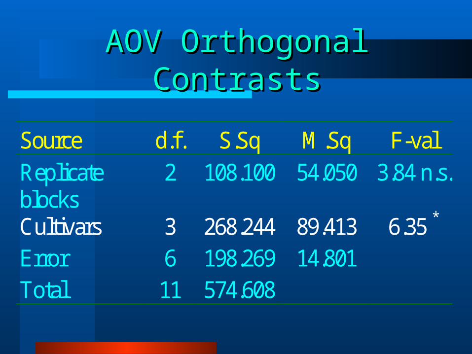
AOV Orthogonal ContrastsAOV Orthogonal Contrasts
Source d.f. S.Sq M.Sq F-valReplicateblocks
2 108.100 54.050 3.84 n.s.
Cultivars 3 268.244 89.413 6.35 *
Error 6 198.269 14.801Total 11 574.608
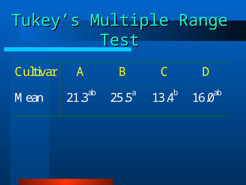
Tukey’s Multiple Range TestTukey’s Multiple Range Test
Cultivar A B C D
Mean 21.3ab 25.5a 13.4b 16.0ab
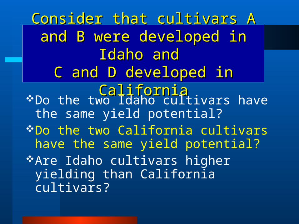
Consider that cultivars A and B were Consider that cultivars A and B were developed in Idaho and developed in Idaho and
C and D developed in CaliforniaC and D developed in California
Do the two Idaho cultivars have the same yield potential?
Do the two California cultivars have the same yield potential?
Are Idaho cultivars higher yielding than California cultivars?
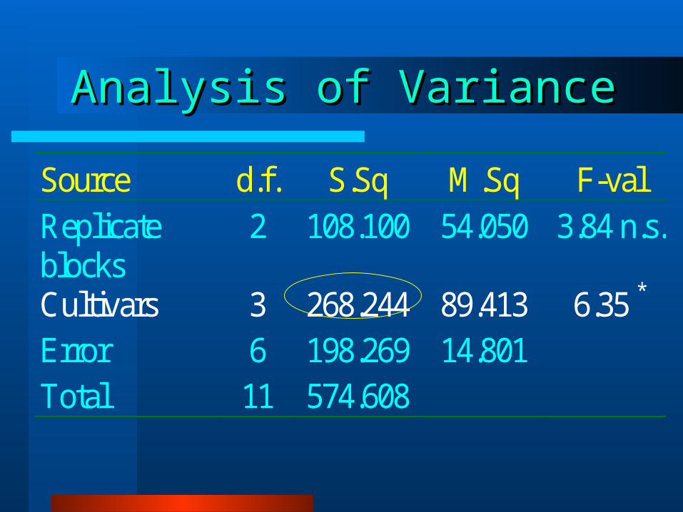
Analysis of VarianceAnalysis of Variance
Source d.f. S.Sq M.Sq F-valReplicateblocks
2 108.100 54.050 3.84 n.s.
Cultivars 3 268.244 89.413 6.35 *
Error 6 198.269 14.801Total 11 574.608
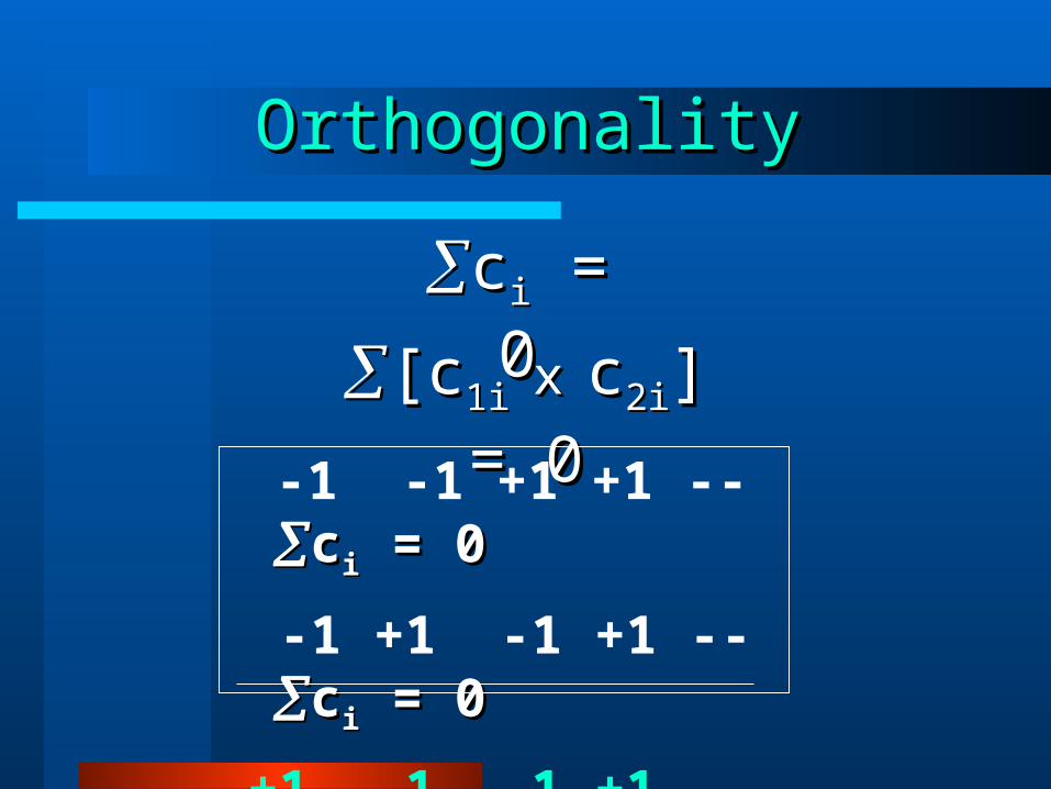
OrthogonalityOrthogonality
ccii = 0 = 0
[c[c1i 1i xx cc2i2i] = 0] = 0
-1 -1 +1 +1 -- ccii = 0 = 0
-1 +1 -1 +1 -- ccii = 0 = 0
+1 -1 -1 +1 -- ccii = 0 = 0
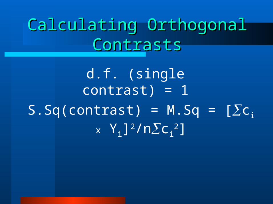
Calculating Orthogonal ContrastsCalculating Orthogonal Contrasts
d.f. (single contrast) = 1
S.Sq(contrast) = M.Sq = [ci x Yi]2/nci2]
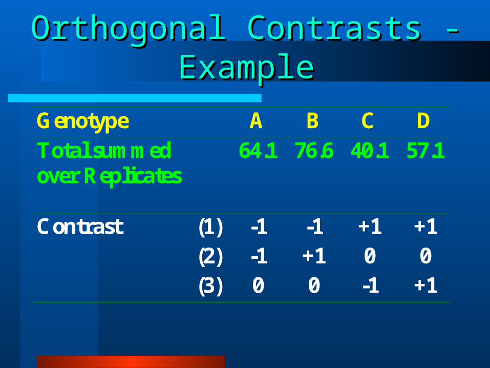
Orthogonal Contrasts - ExampleOrthogonal Contrasts - Example
Genotype A B C D Total summed over Replicates
64.1 76.6 40.1 57.1
Contrast (1) -1 -1 +1 +1 (2) -1 +1 0 0 (3) 0 0 -1 +1
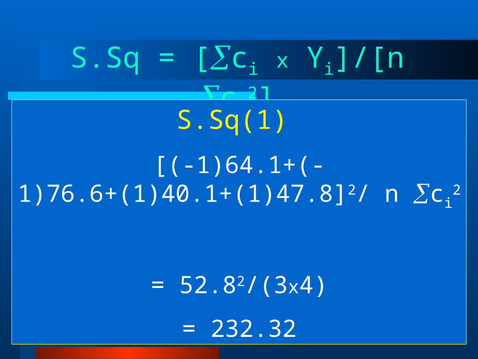
S.Sq = [ci x Yi]/[n ci2]
S.Sq(1)
[(-1)64.1+(-1)76.6+(1)40.1+(1)47.8]2/ n ci2
= 52.82/(3x4)
= 232.32
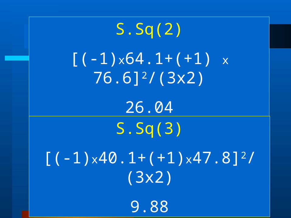
S.Sq(2)
[(-1)x64.1+(+1) x 76.6]2/(3x2)
26.04
S.Sq(3)
[(-1)x40.1+(+1)x47.8]2/(3x2)
9.88
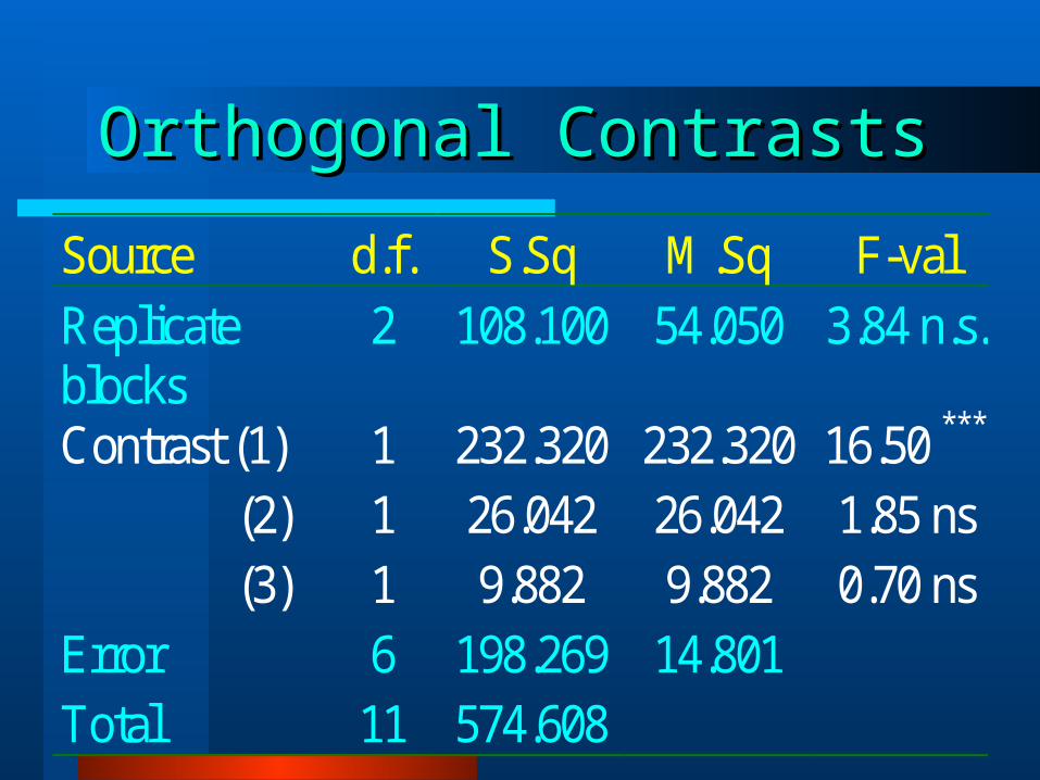
Orthogonal ContrastsOrthogonal Contrasts
Source d.f. S.Sq M.Sq F-valReplicateblocks
2 108.100 54.050 3.84 n.s.
Contrast (1) 1 232.320 232.320 16.50 ***
(2) 1 26.042 26.042 1.85 ns (3) 1 9.882 9.882 0.70 nsError 6 198.269 14.801Total 11 574.608
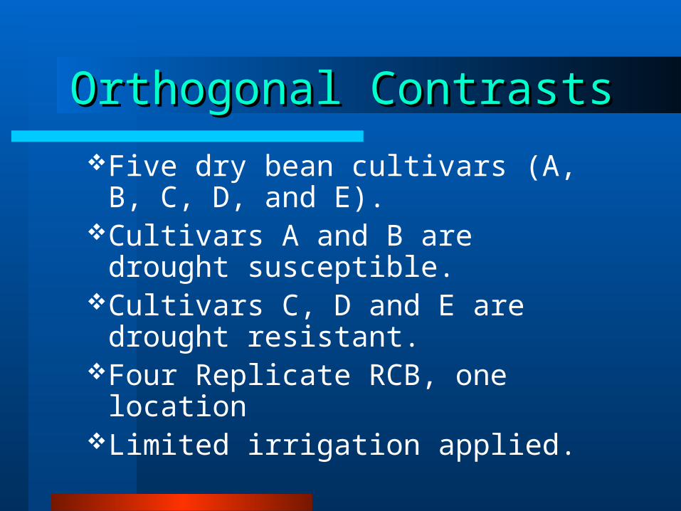
Orthogonal ContrastsOrthogonal Contrasts
Five dry bean cultivars (A, B, C, D, and E).
Cultivars A and B are drought susceptible.
Cultivars C, D and E are drought resistant.
Four Replicate RCB, one locationLimited irrigation applied.
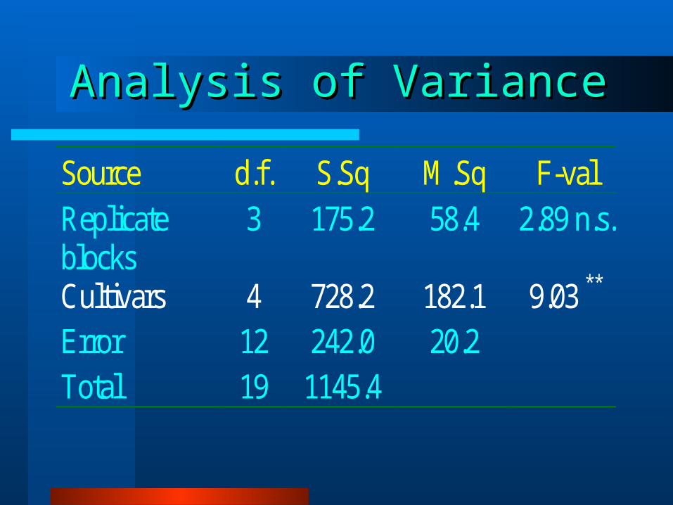
Analysis of VarianceAnalysis of Variance
Source d.f. S.Sq M.Sq F-valReplicateblocks
3 175.2 58.4 2.89 n.s.
Cultivars 4 728.2 182.1 9.03 **
Error 12 242.0 20.2Total 19 1145.4
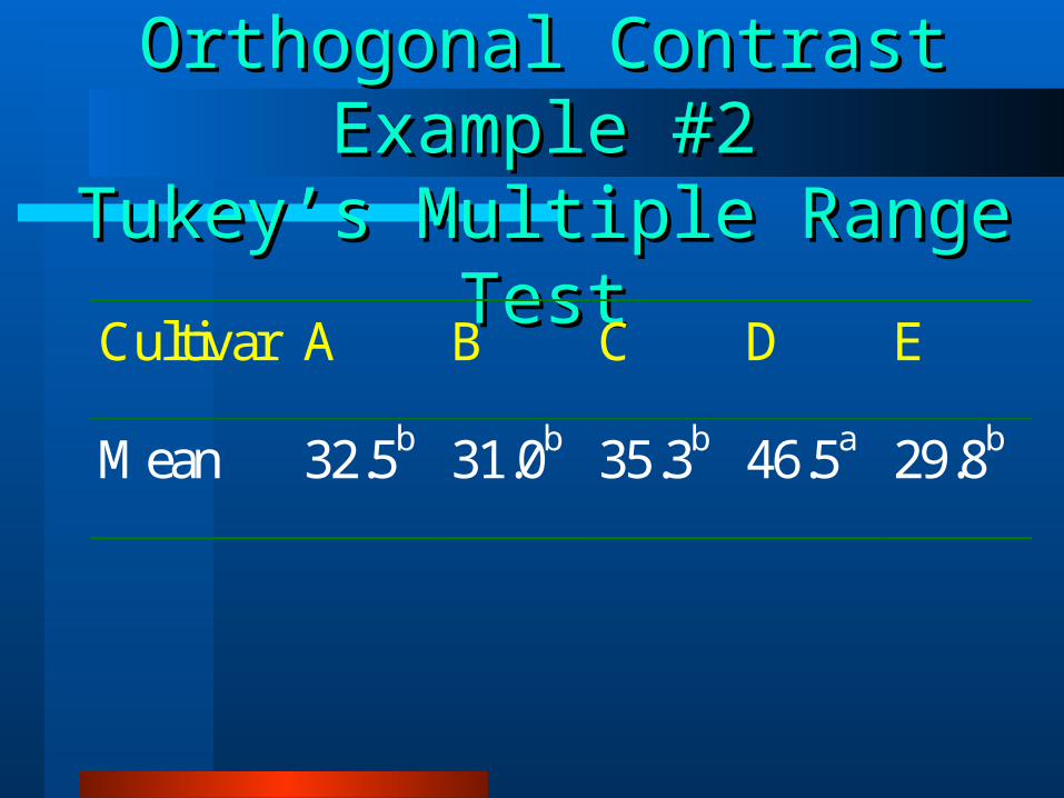
Orthogonal Contrast Example #2Orthogonal Contrast Example #2Tukey’s Multiple Range TestTukey’s Multiple Range Test
Cultivar A B C D E
Mean 32.5b 31.0b 35.3b 46.5a 29.8b
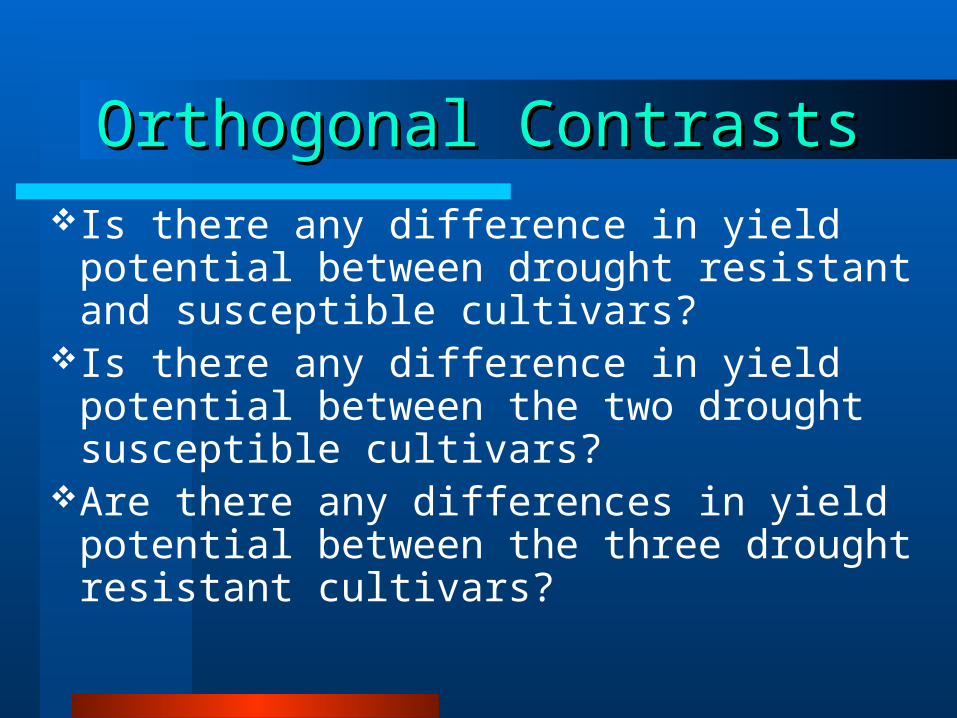
Orthogonal ContrastsOrthogonal ContrastsIs there any difference in yield potential
between drought resistant and susceptible cultivars?
Is there any difference in yield potential between the two drought susceptible cultivars?
Are there any differences in yield potential between the three drought resistant cultivars?
Orthogonal ContrastsOrthogonal Contrasts
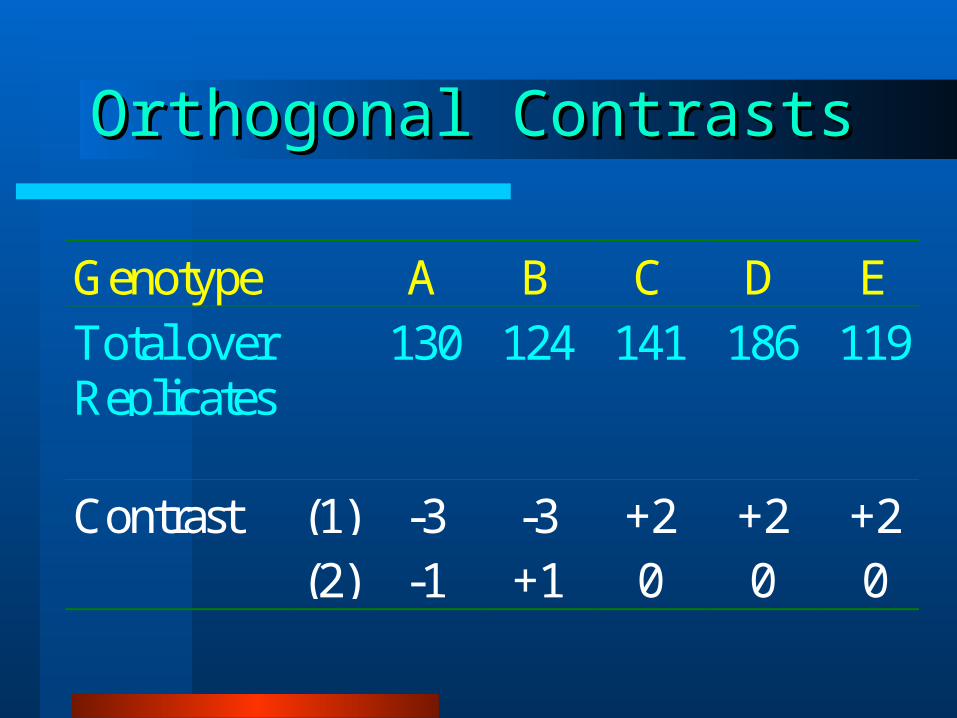
Genotype A B C D ETotal overReplicates
130 124 141 186 119
Contrast (1) -3 -3 +2 +2 +2(2) -1 +1 0 0 0
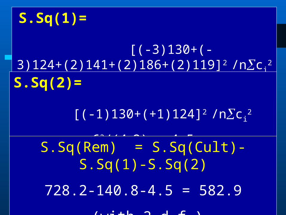
S.Sq(1)= [(-3)130+(-3)124+(2)141+(2)186+(2)119]2 /nci
2
1302/(4x40) = 140.8
S.Sq(2)= [(-1)130+(+1)124]2 /nci
2
62/(4x2) = 4.5
S.Sq(Rem) = S.Sq(Cult)-S.Sq(1)-S.Sq(2)
728.2-140.8-4.5 = 582.9
(with 2 d.f.)
Analysis of VarianceAnalysis of Variance
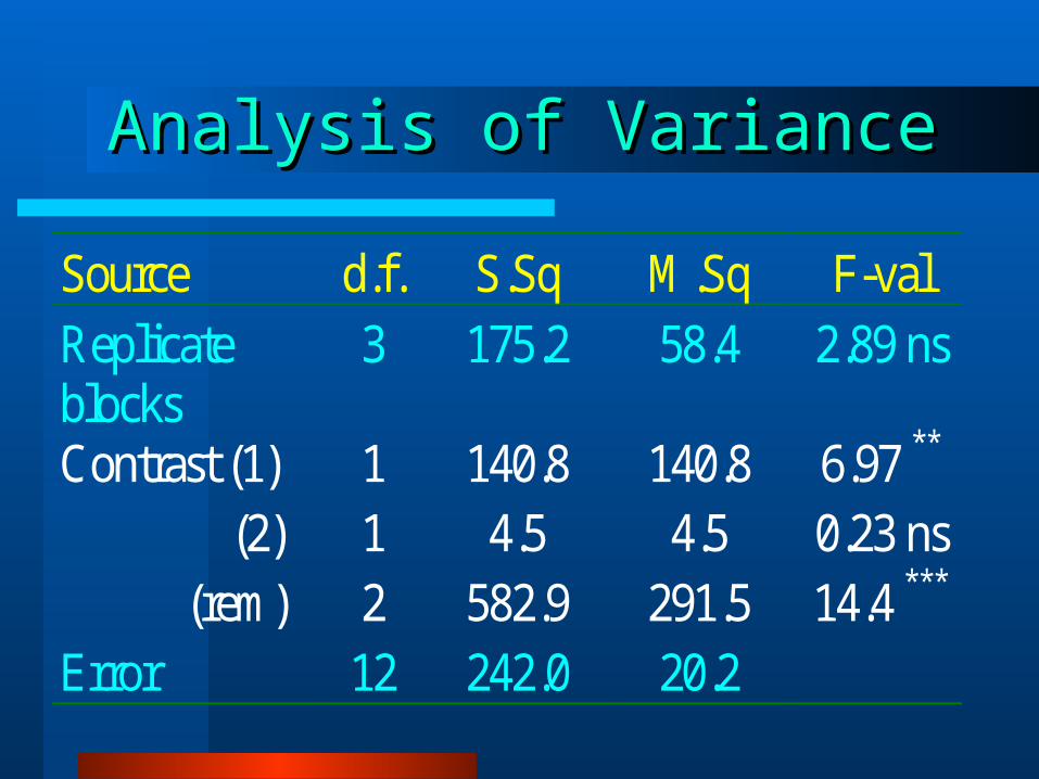
Source d.f. S.Sq M.Sq F-valReplicateblocks
3 175.2 58.4 2.89 ns
Contrast (1) 1 140.8 140.8 6.97 **
(2) 1 4.5 4.5 0.23 ns (rem) 2 582.9 291.5 14.4 ***
Error 12 242.0 20.2
Partition Contrast(rem)Partition Contrast(rem)
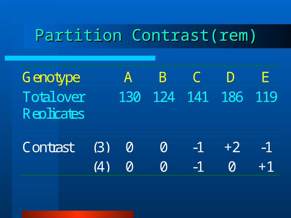
Genotype A B C D ETotal overReplicates
130 124 141 186 119
Contrast (3) 0 0 -1 +2 -1(4) 0 0 -1 0 +1
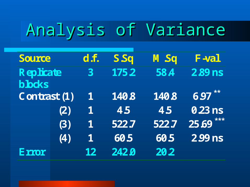
Analysis of VarianceAnalysis of Variance
Source d.f. S.Sq M.Sq F-val Replicate blocks
3 175.2 58.4 2.89 ns
Contrast (1) 1 140.8 140.8 6.97 ** (2) 1 4.5 4.5 0.23 ns (3) 1 522.7 522.7 25.69 *** (4) 1 60.5 60.5 2.99 ns Error 12 242.0 20.2
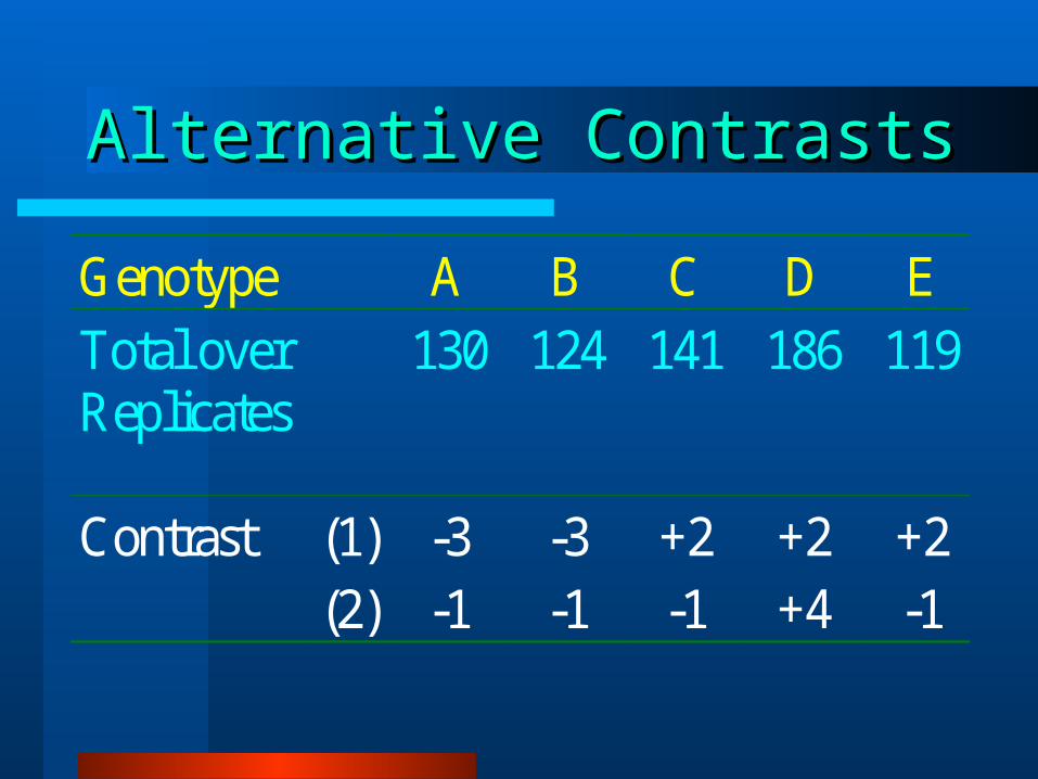
Alternative ContrastsAlternative Contrasts
Genotype A B C D E Total over Replicates
130 124 141 186 119
Contrast (1) -3 -3 +2 +2 +2 (2) -1 -1 -1 +4 -1
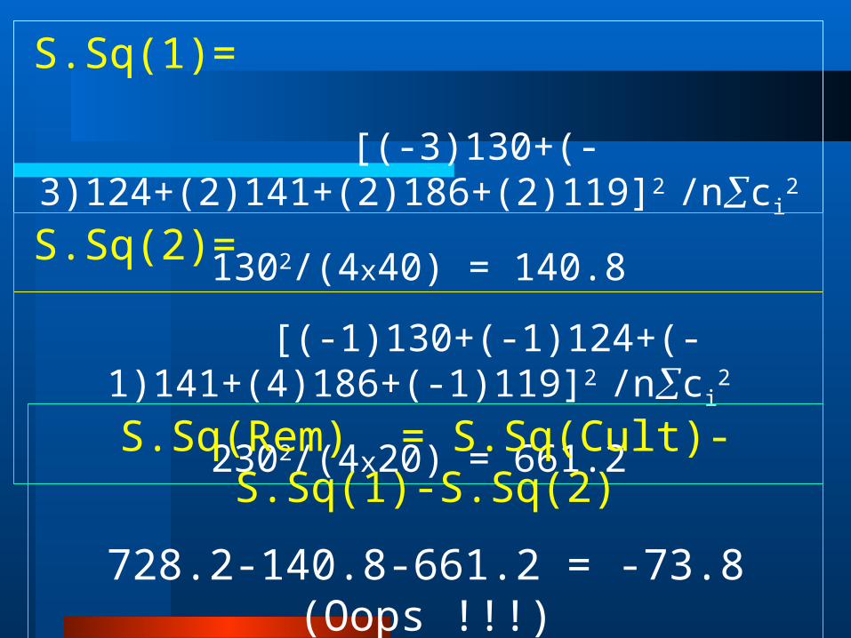
S.Sq(1)= [(-3)130+(-3)124+(2)141+(2)186+(2)119]2 /nci
2
1302/(4x40) = 140.8
S.Sq(2)= [(-1)130+(-1)124+(-1)141+(4)186+(-1)119]2 /nci
2
2302/(4x20) = 661.2
S.Sq(Rem) = S.Sq(Cult)-S.Sq(1)-S.Sq(2)
728.2-140.8-661.2 = -73.8 (Oops !!!)
(with 2 d.f.)
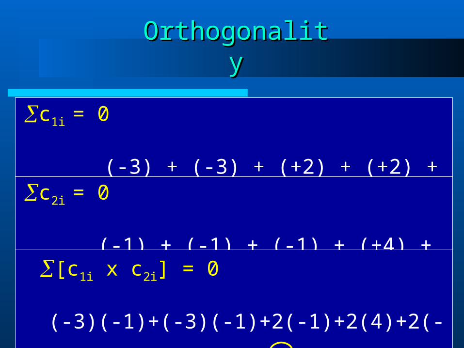
c1i = 0
(-3) + (-3) + (+2) + (+2) + (+2) = 0 = c2i = 0
(-1) + (-1) + (-1) + (+4) + (-1) = 0 = [c1i x c2i] = 0
(-3)(-1)+(-3)(-1)+2(-1)+2(4)+2(-1) =10 =
OrthogonalityOrthogonality
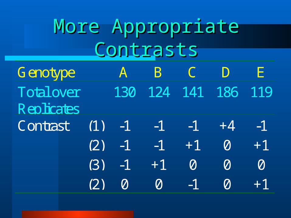
More Appropriate ContrastsMore Appropriate Contrasts
Genotype A B C D ETotal overReplicates
130 124 141 186 119
Contrast (1) -1 -1 -1 +4 -1(2) -1 -1 +1 0 +1(3) -1 +1 0 0 0(2) 0 0 -1 0 +1
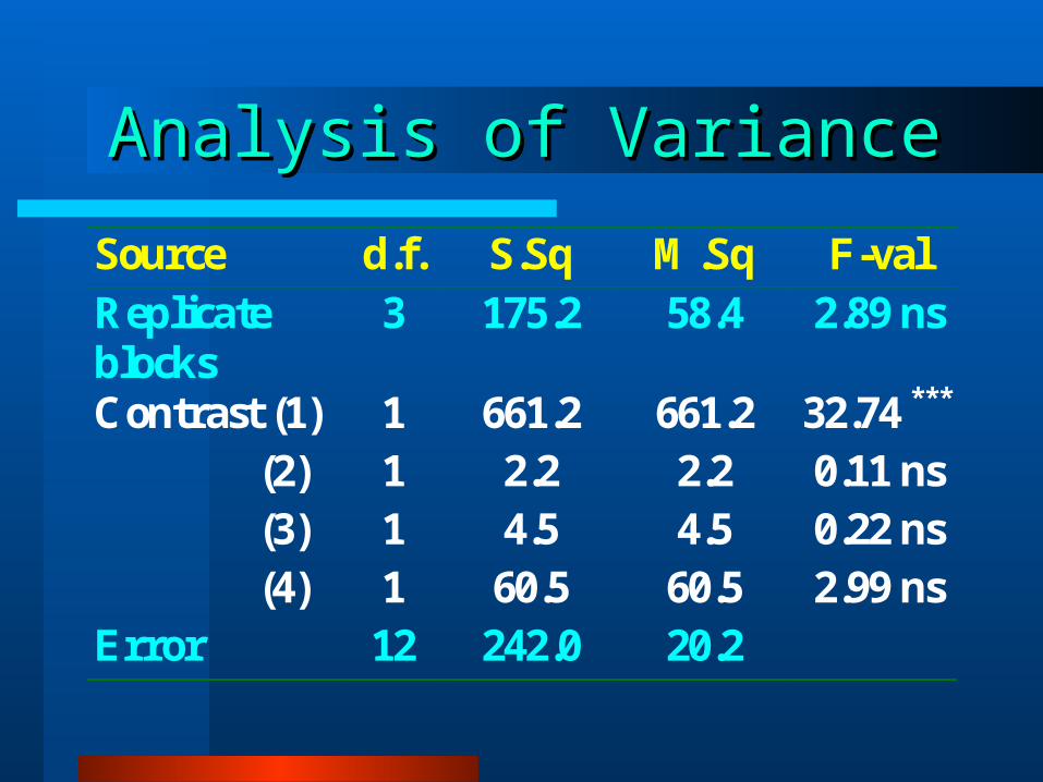
Analysis of VarianceAnalysis of Variance
Source d.f. S.Sq M.Sq F-val Replicate blocks
3 175.2 58.4 2.89 ns
Contrast (1) 1 661.2 661.2 32.74 *** (2) 1 2.2 2.2 0.11 ns (3) 1 4.5 4.5 0.22 ns (4) 1 60.5 60.5 2.99 ns Error 12 242.0 20.2
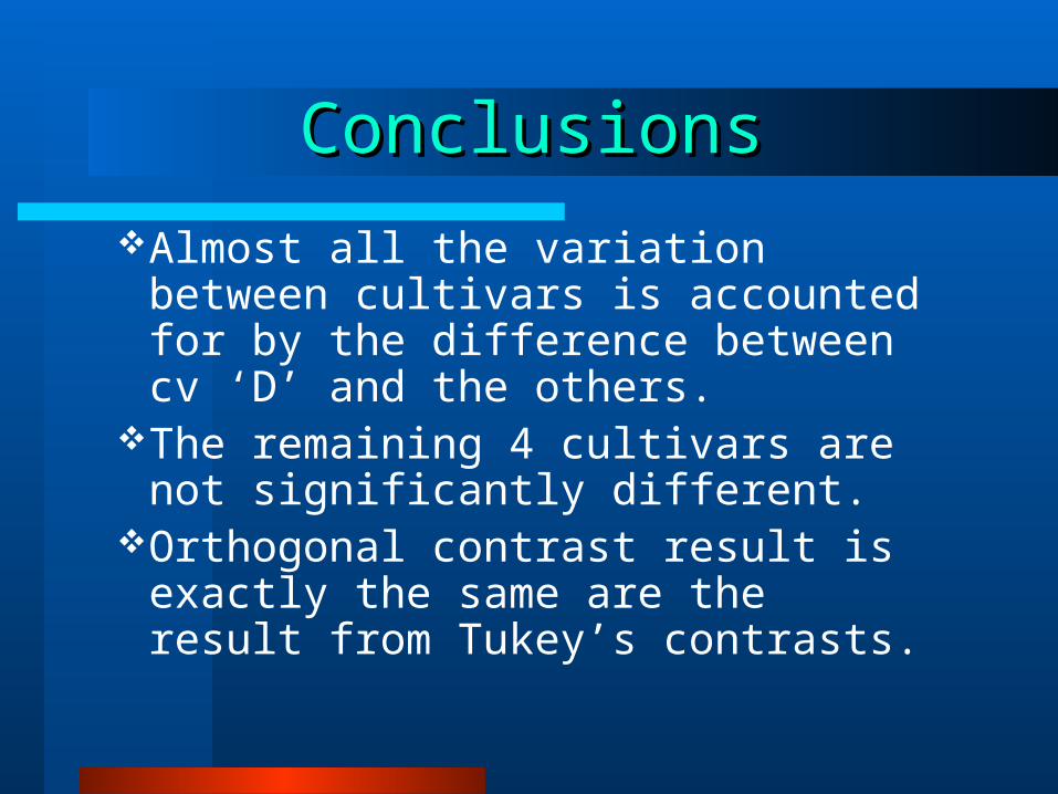
ConclusionsConclusions
Almost all the variation between cultivars is accounted for by the difference between cv ‘D’ and the others.
The remaining 4 cultivars are not significantly different.
Orthogonal contrast result is exactly the same are the result from Tukey’s contrasts.
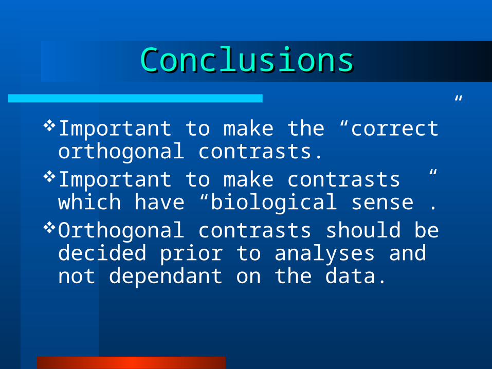
ConclusionsConclusions
Important to make the “correct” orthogonal contrasts.
Important to make contrasts which have “biological sense”.
Orthogonal contrasts should be decided prior to analyses and not dependant on the data.
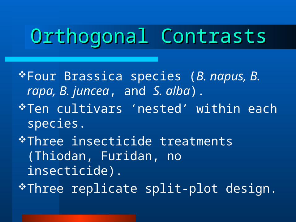
Orthogonal ContrastsOrthogonal Contrasts
Four Brassica species (B. napus, B. rapa, B. juncea, and S. alba).
Ten cultivars ‘nested’ within each species.
Three insecticide treatments (Thiodan, Furidan, no insecticide).
Three replicate split-plot design.
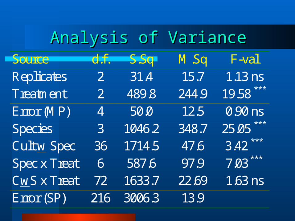
Analysis of VarianceAnalysis of VarianceSource d.f. S.Sq M.Sq F-val Replicates 2 31.4 15.7 1.13 ns Treatment 2 489.8 244.9 19.58 *** Error (MP) 4 50.0 12.5 0.90 ns Species 3 1046.2 348.7 25.05 *** Cult w Spec 36 1714.5 47.6 3.42 *** Spec x Treat 6 587.6 97.9 7.03 *** CwS x Treat 72 1633.7 22.69 1.63 ns Error (SP) 216 3006.3 13.9
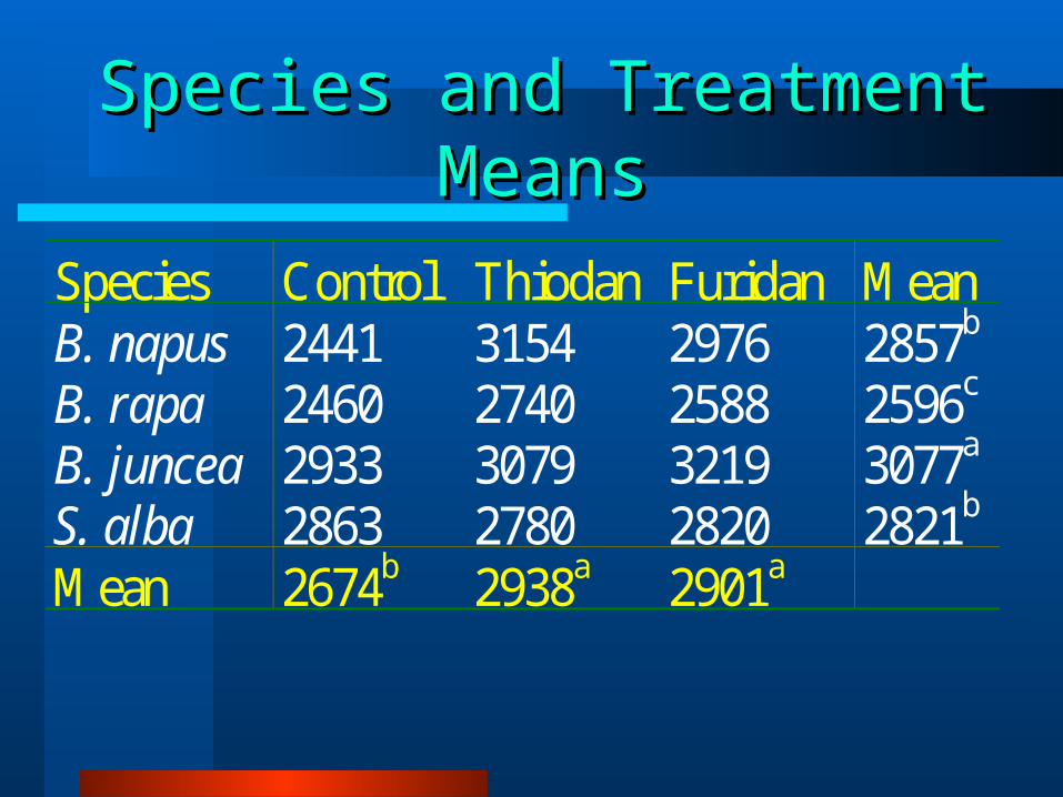
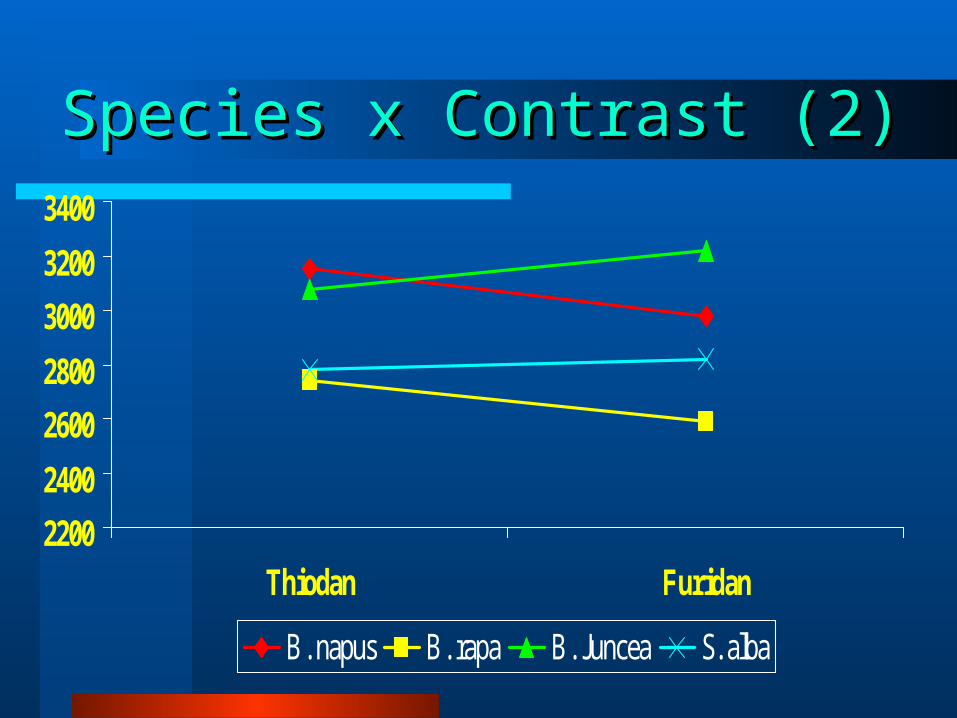
Species and Treatment MeansSpecies and Treatment Means
Species Control Thiodan Furidan MeanB. napus 2441 3154 2976 2857b
B. rapa 2460 2740 2588 2596c
B. juncea 2933 3079 3219 3077a
S. alba 2863 2780 2820 2821b
Mean 2674b 2938a 2901a
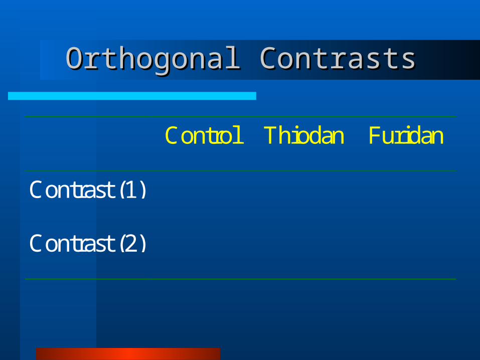
Control Thiodan Furidan
Contrast (1)
Contrast (2)
Orthogonal ContrastsOrthogonal Contrasts
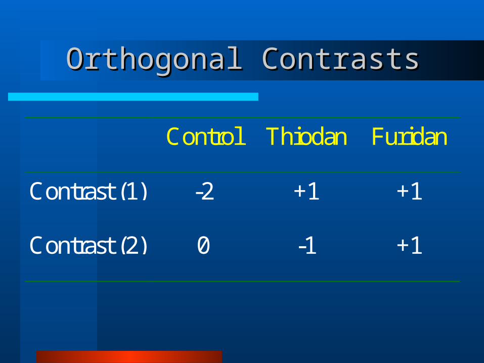
Control Thiodan Furidan
Contrast (1) -2 +1 +1
Contrast (2) 0 -1 +1
Orthogonal ContrastsOrthogonal Contrasts
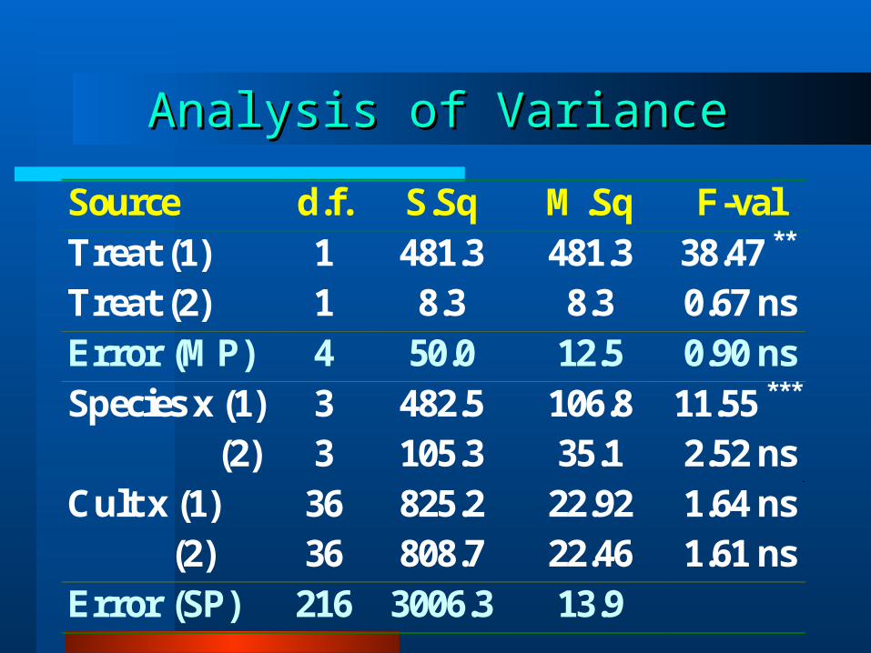
Analysis of VarianceAnalysis of Variance
Source d.f. S.Sq M.Sq F-val Treat (1) 1 481.3 481.3 38.47 ** Treat (2) 1 8.3 8.3 0.67 ns Error (MP) 4 50.0 12.5 0.90 ns Species x (1) 3 482.5 106.8 11.55 *** (2) 3 105.3 35.1 2.52 ns Cult x (1) 36 825.2 22.92 1.64 ns (2) 36 808.7 22.46 1.61 ns Error (SP) 216 3006.3 13.9
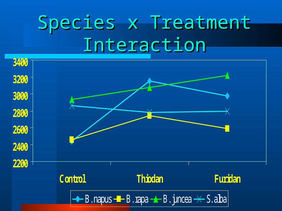
Species x Treatment InteractionSpecies x Treatment Interaction
2200
2400
2600
2800
3000
3200
3400
Control Thiodan Furidan
B. napus B. rapa B. juncea S. alba
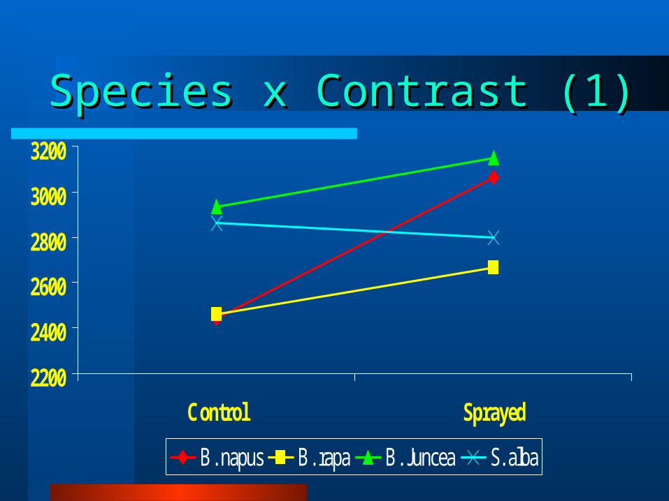
Species x Contrast (1)Species x Contrast (1)
2200
2400
2600
2800
3000
3200
Control Sprayed
B. napus B. rapa B. Juncea S. alba
Species x Contrast (2)Species x Contrast (2)
2200
2400
2600
2800
3000
3200
3400
Thiodan Furidan
B. napus B. rapa B. Juncea S. alba
Orthogonal Contrasts and InteractionsOrthogonal Contrasts and Interactions
Consider a cross classified factorial design with 4 replicates.
Four cultivars; 2 from Idaho and 2 from California (again).
3 herbicide treatments; No-treatment control, Killall, and Onllik.
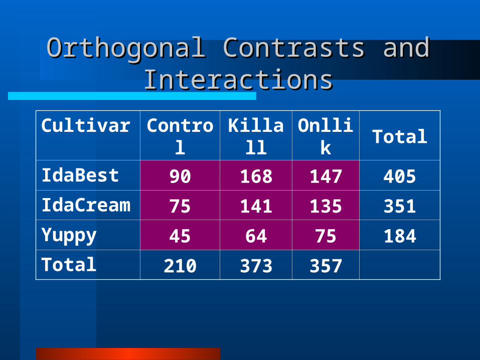
Cultivar Control Killall Onllik Total
IdaBest 90 168 147 405
IdaCream 75 141 135 351
Yuppy 45 64 75 184
Total 210 373 357
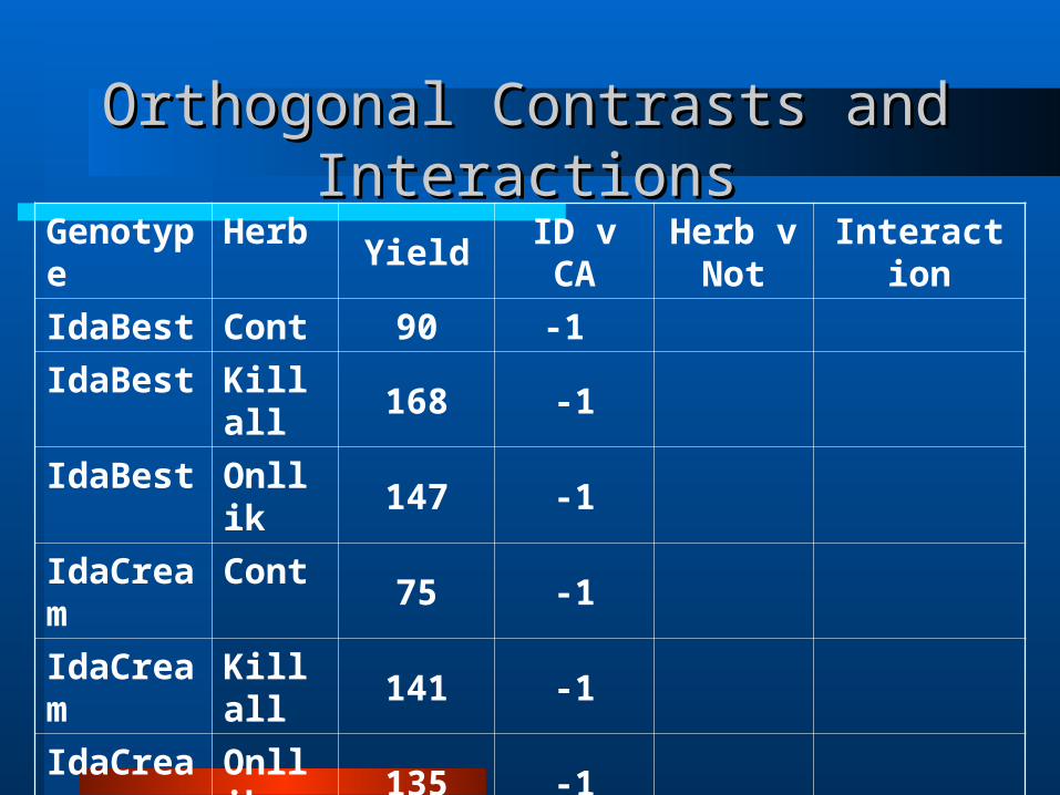
Orthogonal Contrasts and InteractionsOrthogonal Contrasts and Interactions
Orthogonal Contrasts and InteractionsOrthogonal Contrasts and Interactions
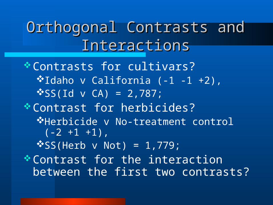
Contrasts for cultivars?Idaho v California (-1 -1 +2),SS(Id v CA) = 2,787;
Contrast for herbicides?Herbicide v No-treatment control (-2 +1 +1),SS(Herb v Not) = 1,779;
Contrast for the interaction between the first two contrasts?

Genotype HerbYield ID v CA
Herb v Not
Interaction
IdaBest Cont 90
IdaBest Killall 168
IdaBest Onllik 147
IdaCream Cont 75
IdaCream Killall 141
IdaCream Onllik 135
Yuppy Cont 45
Yuppy Killall 64
Yuppy Onllik 75
Orthogonal Contrasts and InteractionsOrthogonal Contrasts and Interactions
Genotype HerbYield ID v CA
Herb v Not
Interaction
IdaBest Cont 90 -1
IdaBest Killall 168 -1
IdaBest Onllik 147 -1
IdaCream Cont 75 -1
IdaCream Killall 141 -1
IdaCream Onllik 135 -1
Yuppy Cont 45 +2
Yuppy Killall 64 +2
Yuppy Onllik 75 +2
Orthogonal Contrasts and InteractionsOrthogonal Contrasts and Interactions
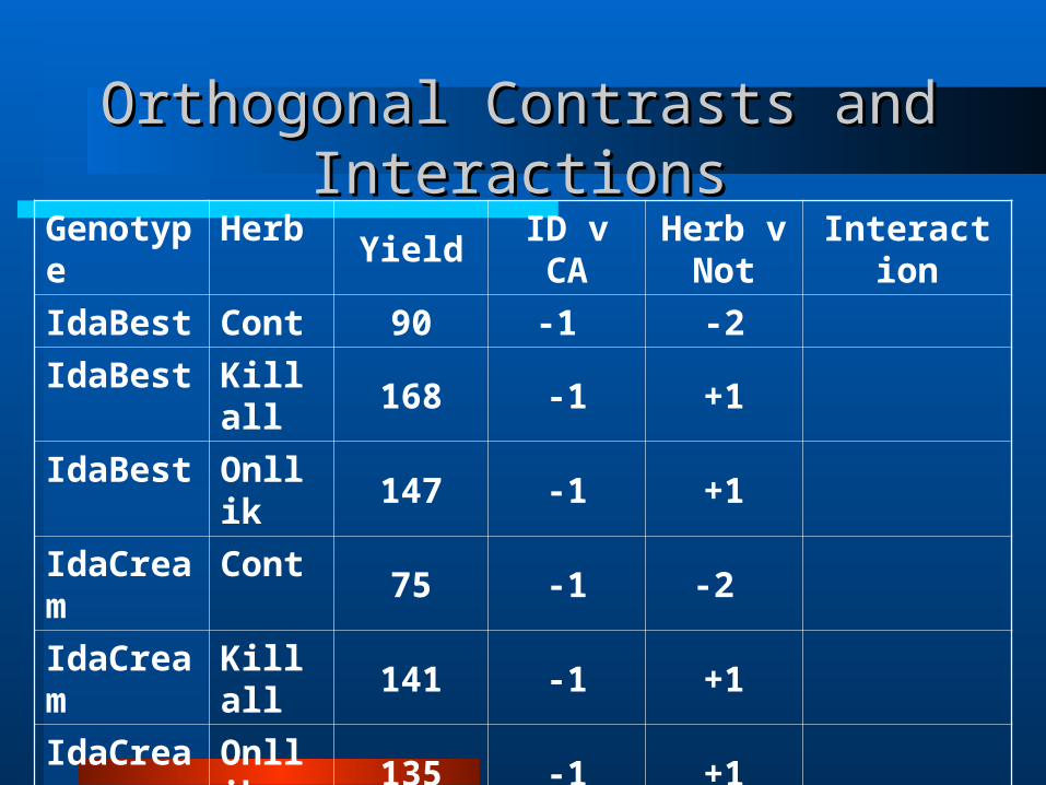
Genotype HerbYield ID v CA
Herb v Not
Interaction
IdaBest Cont 90 -1 -2
IdaBest Killall 168 -1 +1
IdaBest Onllik 147 -1 +1
IdaCream Cont 75 -1 -2
IdaCream Killall 141 -1 +1
IdaCream Onllik 135 -1 +1
Yuppy Cont 45 +2 -2
Yuppy Killall 64 +2 +1
Yuppy Onllik 75 +2 +1
Orthogonal Contrasts and InteractionsOrthogonal Contrasts and Interactions
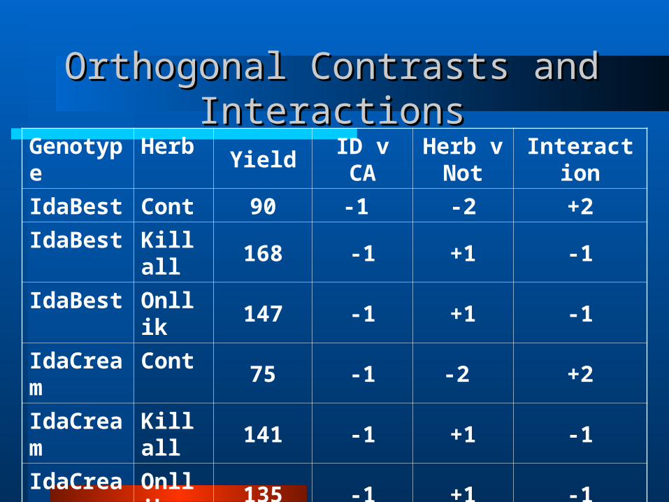
Genotype HerbYield ID v CA
Herb v Not
Interaction
IdaBest Cont 90 -1 -2 +2
IdaBest Killall 168 -1 +1 -1
IdaBest Onllik 147 -1 +1 -1
IdaCream Cont 75 -1 -2 +2
IdaCream Killall 141 -1 +1 -1
IdaCream Onllik 135 -1 +1 -1
Yuppy Cont 45 +2 -2 -4
Yuppy Killall 64 +2 +1 +2
Yuppy Onllik 75 +2 +1 +2
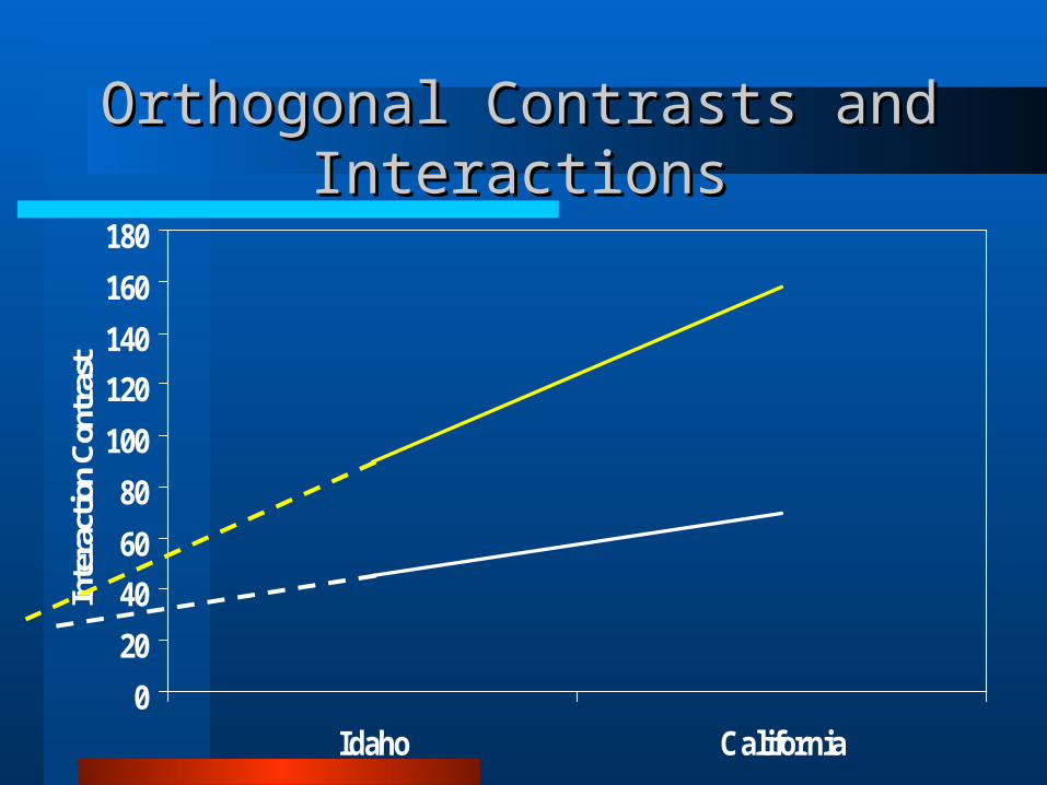
Orthogonal Contrasts and InteractionsOrthogonal Contrasts and Interactions

Orthogonal Contrasts and InteractionsOrthogonal Contrasts and Interactions
Contrasts for cultivars?Idaho v California (-1 -1 +2),SS(Id v CA) = 2,787;
Contrast for herbicides?Herbicide v No-treatment control (-2 +1 +1),SS(Herb v Not) = 1,779;
Contrast for the interaction between the first two contrasts?SS (Interaction) = 246.
0
20
40
60
80
100
120
140
160
180
Idaho California
Inte
ract
ion
Con
tras
t
Orthogonal Contrasts and InteractionsOrthogonal Contrasts and Interactions
More Orthogonal Contrasts More Orthogonal Contrasts …… Trend AnalysesTrend Analyses

Aim of Analyses of VarianceAim of Analyses of Variance
Detect significant differences between treatment means.
Determine trends that may exist as a result of varying specific factor levels.
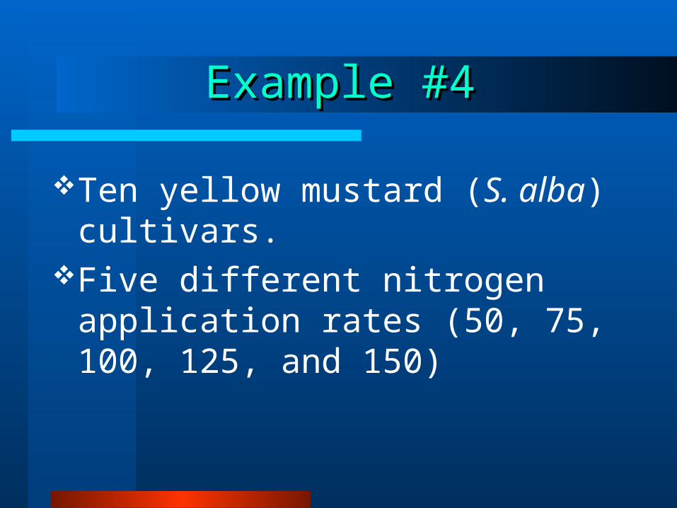
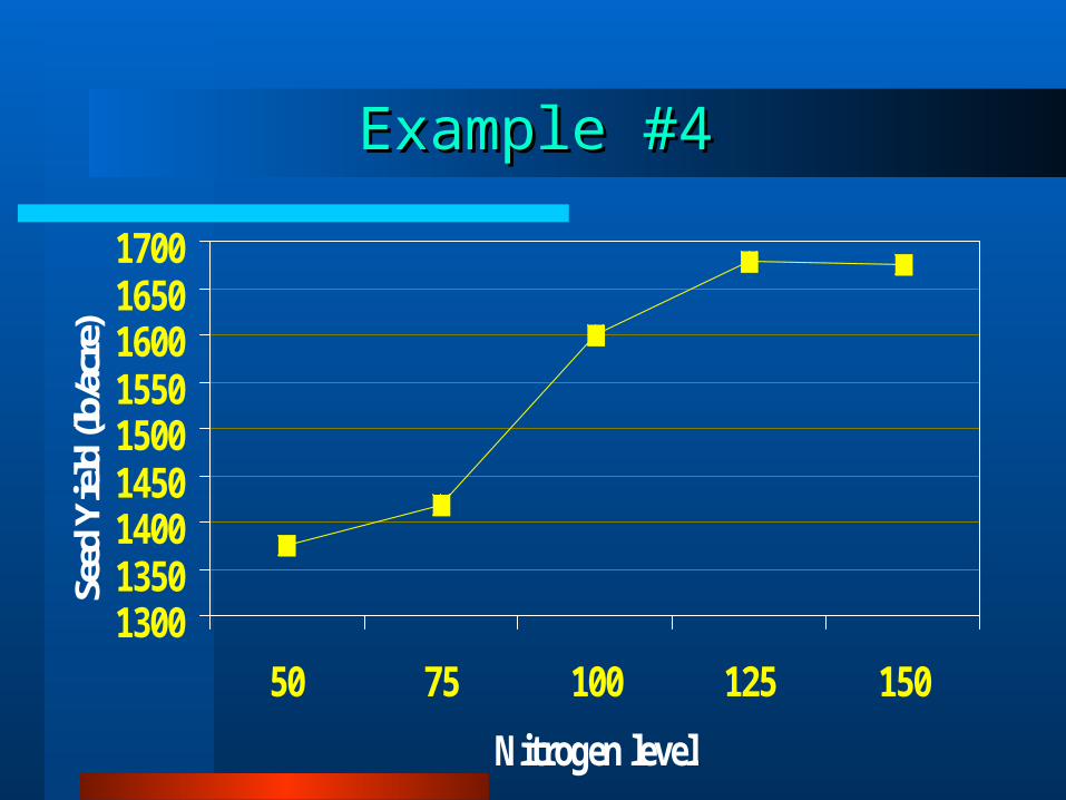
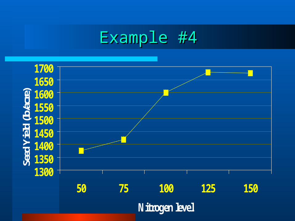
Example #4Example #4
Ten yellow mustard (S. alba) cultivars.Five different nitrogen application rates
(50, 75, 100, 125, and 150)
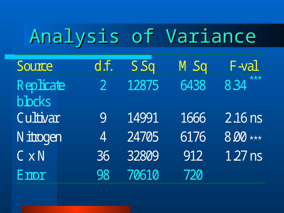
Analysis of VarianceAnalysis of VarianceSource d.f. S.Sq M.Sq F-valReplicateblocks
2 12875 6438 8.34 ***
Cultivar 9 14991 1666 2.16 nsNitrogen 4 24705 6176 8.00 ***
C x N 36 32809 912 1.27 nsError 98 70610 720
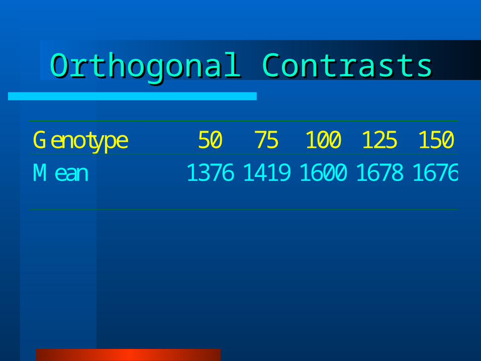
Orthogonal ContrastsOrthogonal Contrasts
Genotype 50 75 100 125 150Mean 1376 1419 1600 1678 1676
Example #4Example #4
130013501400145015001550160016501700
50 75 100 125 150
Nitrogen level
Seed
Yie
ld (l
b/ac
re)
Example #4Example #4
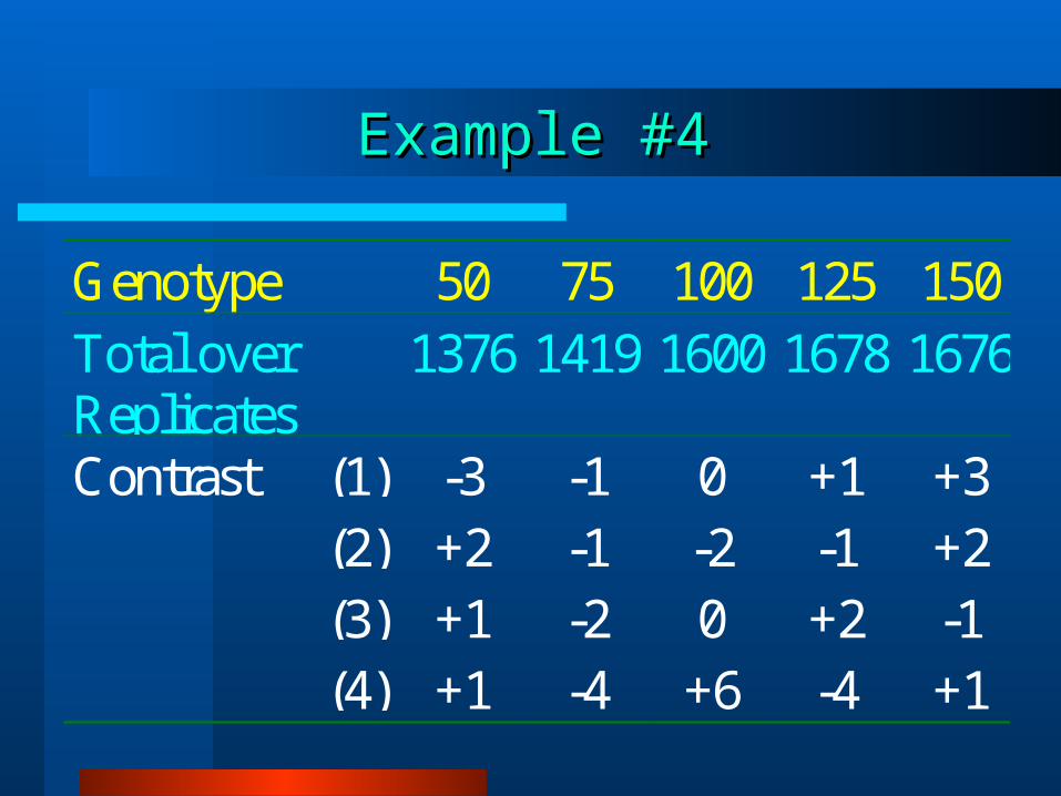
Genotype 50 75 100 125 150Total overReplicates
1376 1419 1600 1678 1676
Contrast (1) -3 -1 0 +1 +3(2) +2 -1 -2 -1 +2(3) +1 -2 0 +2 -1(4) +1 -4 +6 -4 +1
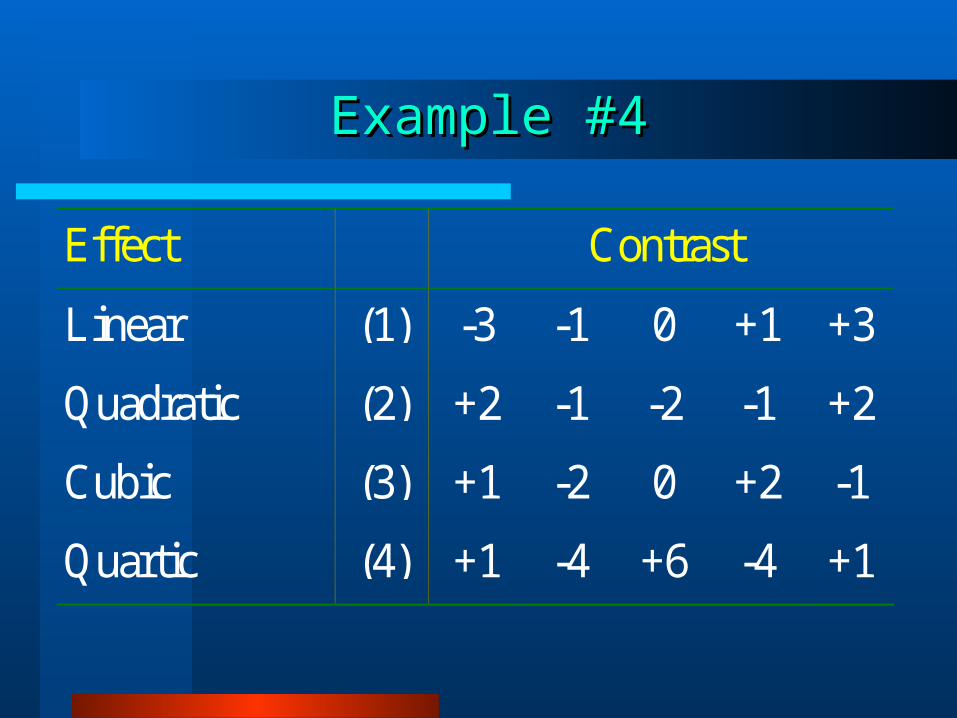
Example #4Example #4
Effect Contrast
Linear (1) -3 -1 0 +1 +3
Quadratic (2) +2 -1 -2 -1 +2
Cubic (3) +1 -2 0 +2 -1
Quartic (4) +1 -4 +6 -4 +1
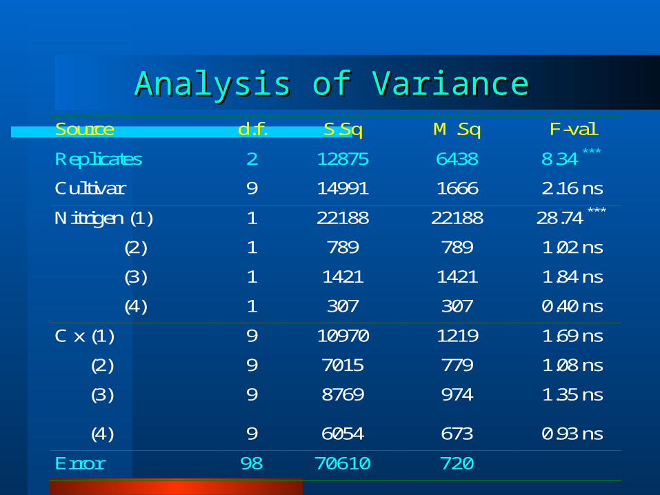
Analysis of VarianceAnalysis of VarianceSource d.f. S.Sq M.Sq F-val
Replicates 2 12875 6438 8.34 ***
Cultivar 9 14991 1666 2.16 ns
Nitrigen (1) 1 22188 22188 28.74 ***
(2) 1 789 789 1.02 ns
(3) 1 1421 1421 1.84 ns
(4) 1 307 307 0.40 ns
C x (1) 9 10970 1219 1.69 ns
(2) 9 7015 779 1.08 ns
(3) 9 8769 974 1.35 ns
(4) 9 6054 673 0.93 ns
Error 98 70610 720

Trend AnalysesTrend Analyses
The F-value associates with a trend contrast is significant.
All higher order trend contrasts are not significant.
Example #4Example #4
130013501400145015001550160016501700
50 75 100 125 150
Nitrogen level
Seed
Yie
ld (l
b/ac
re)
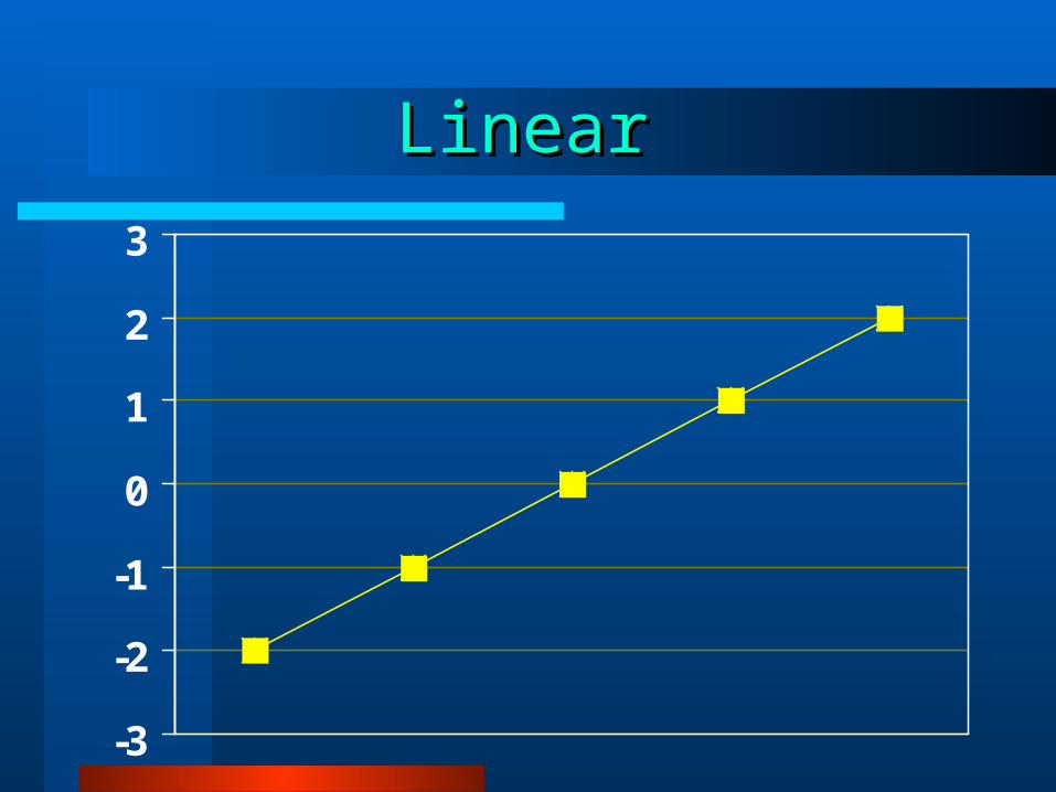
LinearLinear
-3
-2
-1
0
1
2
3
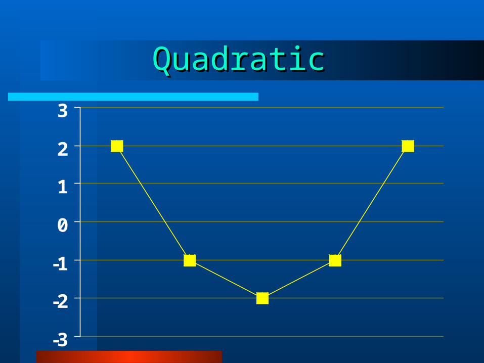
QuadraticQuadratic
-3
-2
-1
0
1
2
3
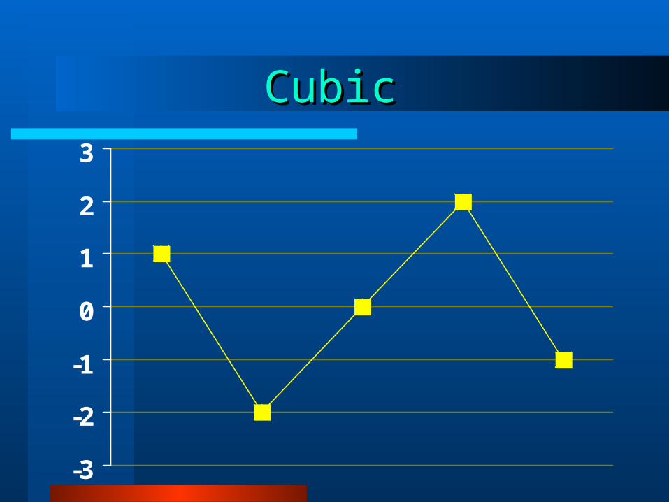
CubicCubic
-3
-2
-1
0
1
2
3
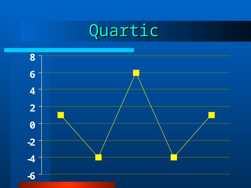
QuarticQuartic
-6
-4
-2
0
2
4
6
8
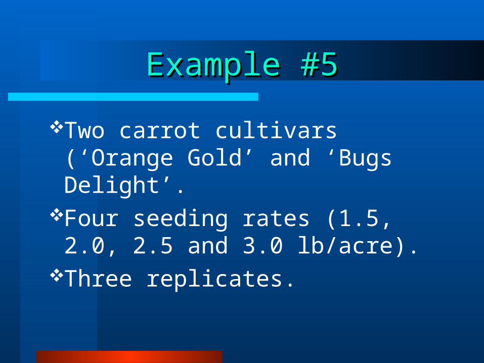
Example #5Example #5
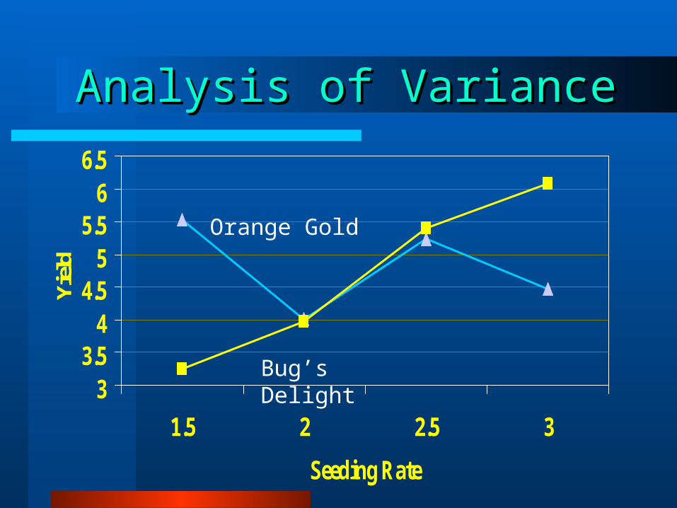
Two carrot cultivars (‘Orange Gold’ and ‘Bugs Delight’.
Four seeding rates (1.5, 2.0, 2.5 and 3.0 lb/acre).
Three replicates.
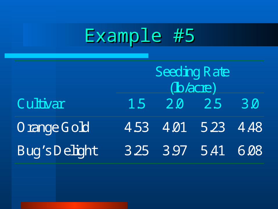
Example #5Example #5
Seeding Rate(lb/acre)
Cultivar 1.5 2.0 2.5 3.0
Orange Gold 4.53 4.01 5.23 4.48
Bug’s Delight 3.25 3.97 5.41 6.08
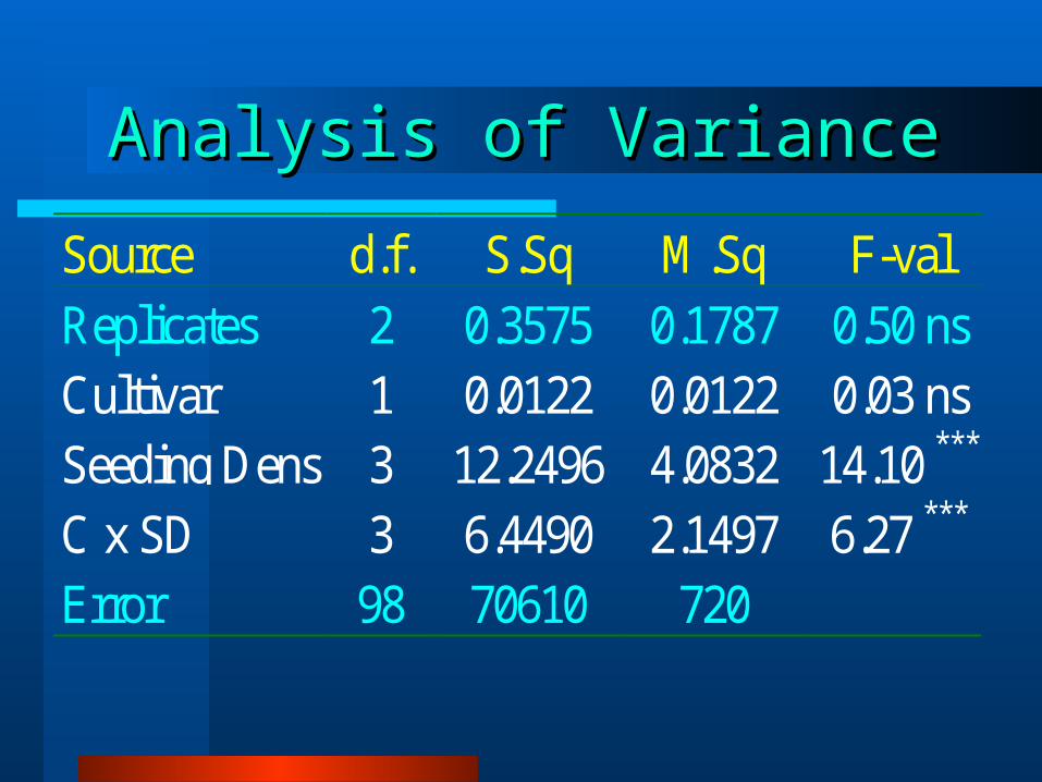
Analysis of VarianceAnalysis of Variance
Source d.f. S.Sq M.Sq F-valReplicates 2 0.3575 0.1787 0.50 nsCultivar 1 0.0122 0.0122 0.03 nsSeeding Dens 3 12.2496 4.0832 14.10 ***
C x SD 3 6.4490 2.1497 6.27 ***
Error 98 70610 720
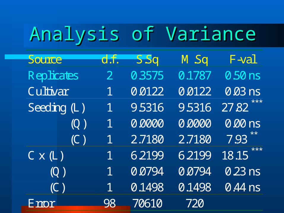
Analysis of VarianceAnalysis of VarianceSource d.f. S.Sq M.Sq F-valReplicates 2 0.3575 0.1787 0.50 nsCultivar 1 0.0122 0.0122 0.03 nsSeeding (L) 1 9.5316 9.5316 27.82 ***
(Q) 1 0.0000 0.0000 0.00 ns (C) 1 2.7180 2.7180 7.93 **
C x (L) 1 6.2199 6.2199 18.15 ***
(Q) 1 0.0794 0.0794 0.23 ns (C) 1 0.1498 0.1498 0.44 nsError 98 70610 720
Analysis of VarianceAnalysis of Variance
33.5
44.5
55.5
66.5
1.5 2 2.5 3
Seeding Rate
Yield
Orange Gold
Bug’s Delight

End of Analyses of End of Analyses of Variance SectionVariance Section


