Page 1
Thesis Presentation: April 30, 2003 1
Multiple Correspondence Analysis in
Marketing Research
Yangchun Du
Advisor: John C. Kern II
Department of Mathematics and Computer Science
Duquesne University
April 30, 2003
Page 2
Thesis Presentation: April 30, 2003 2
Outline
1. Introduction
2. Background
3. Details of Method
4. Simulated Data
5. MCA Properties
6. MSA Data
7. Conclusion and Future Work
8. References
9. S-Plus Code
Page 3
Thesis Presentation: April 30, 2003 3
Introduction
Correspondence Analysis: A descriptive/exploratory
technique to analyze simple two-way and multi-way
tables containing some measure of correspondence
between the rows and columns.
Goal: Convert the numerical information from a
contingency table into a two-dimensional graphical
display.
Data Type: Categorical Data.
Application Area: Marketing Research.
Advantage: Allowing researcher to visualize relationships
among categories of categorical variables for large data
sets.
Page 4
Thesis Presentation: April 30, 2003 4
Introduction (continued)
Multiple Correspondence Analysis (MCA) is considered
to be an extension of simple correspondence analysis to
more than Q = 2 variables.
Indicator matrix Z (n × ∑
q Jq)
Row—individuals (usually people).
Column—category of a categorical variable.
Z=
male female location1 location2
1 0 1 0
1 0 0 1
0 1 1 0
0 1 0 1
0 1 0 1
Burt Matrix B = Zt × Z
B=
male female location1 location2
male 2 0 1 1
female 0 3 1 2
location1 1 1 2 0
location2 1 2 0 3
Page 5
Thesis Presentation: April 30, 2003 5
Background
Computation for Simple Correspondence Analysis
Let N be a I × J matrix representing a contingency
table of two categorical variables.
• Row mass ri : row sums divided by grand total n,
ri = ni+
n ; vector of row masses r .
• Column mass cj : column sums divided by grand
total n, cj =n+j
n ; vector of column masses c .
• Correspondence Matrix P: original table N divided
by grand total n, P = N
n .
• Row profiles: rows of the original table N divided
by respective row totals; equivalently D−1r P, where
Dr is diagonal matrix of row masses.
• Column profiles: columns of the original table N
divided by respective column totals; equivalently
PD−1c , where Dc is diagonal matrix of column
masses.
• Standardized Residuals: I × J matrix A with
elements aij =pij−ricj√
ricj; A = D−1/2
r (P − rcT )D−1/2c .
Page 6
Thesis Presentation: April 30, 2003 6
• Singular Value Decomposition(SVD) of I × J matrix
A into product of three matrices:
A = UΓVT ,
Γ diagonal matrix γ11 ≥ γ22 ≥ · · · ≥ γkk > 0 (these
are singular values); columns of matrices U and V
are left and right singular vectors, respectively.
• Chi-square statistic: χ2 = n∑
i
∑
j a2ij .
• Total Inertia:∑
i
∑
j a2ij . Equivalently χ2
n .
• Maximum K dimensions for graphical display in
CA, where K = min{I − 1, J − 1}. Squares of
singular values of A also decompose total inertia:
λ1 . . . λk, are principal inertias.
Greenacre (1984) shows that the correspondence
analysis of the indicator matrix Z are identical
to those in the analysis of B. Furthermore, the
principal inertias of B are squares of those of Z.
• The principal coordinates of the rows are obtained
as D−1/2r UΓ.
• The principal coordinates of the columns are
obtained as D−1/2c VΓ.
Page 7
Thesis Presentation: April 30, 2003 7
Details of Method
• Currently, some statistical software packages can
perform MCA.
– SAS: built-in corresp procedure
– SPSS Categories: CA procedure
Commonality: Decompose Burt matrix using SVD.
• Greenacre (1988)
– Creates modified Burt matrix— the original
Burt matrix with modified sub-matrices on its
diagonal
– Advantage (over standard MCA analysis):
greater percentage of explained variation (total
inertia) by two-dimensional solution for some
categorical datasets.
Page 8
Thesis Presentation: April 30, 2003 8
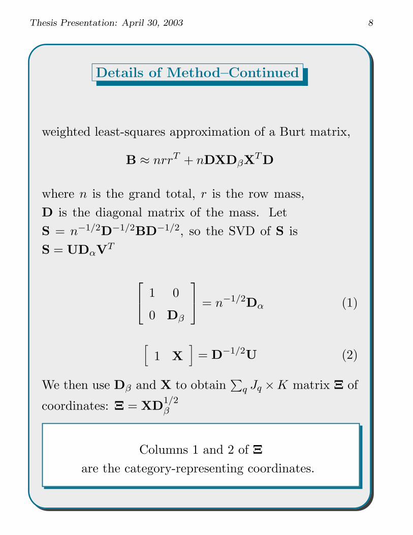
Details of Method–Continued
weighted least-squares approximation of a Burt matrix,
B ≈ nrrT + nDXDβXTD
where n is the grand total, r is the row mass,
D is the diagonal matrix of the mass. Let
S = n−1/2D−1/2BD−1/2, so the SVD of S is
S = UDαVT
1 0
0 Dβ
= n−1/2Dα (1)
[
1 X
]
= D−1/2
U (2)
We then use Dβ and X to obtain∑
q Jq ×K matrix Ξ of
coordinates: Ξ = XD1/2β
Columns 1 and 2 of Ξ
are the category-representing coordinates.
Page 9
Thesis Presentation: April 30, 2003 9
We build a model for the whole matrix B − nrrT ,
namely
B − nrrT ≈ nDXDβXTD + C
where C is a block diagonal matrix with sub-matrices
Cqq (q = 1, ...Q) down the diagonal and zeros elsewhere.
So, the new sub-matrix N∗qq on the diagonal of B∗,
which is given by
N∗qq = nrqr
Tq + nDqXqDβXT
q Dq, (3)
has the same row and column margins as Nqq. where the
vector of Jq masses for variable q is denoted by rq.The
Jq ×Jq diagonal matrix formed from the elements of rq is
now denoted by Dq. Meanwhile, the diagonal m matrix
Dβ contains a scale parameter for each dimension. The
parameter X is partitioned two-wise according to the
variable as X1 · · ·XQ. so Xq is a Jq × K sub matrices.
The procedure of this algorithm:
1. Start with a solution for X and Dβ based on MCA.
2. Replace the sub matrices on the diagonal of B with
those “estimated” by X and Dβ given by (3).
3. Perform a correspondence analysis on the modified
matrix B∗, setting X equal to the first K vectors of
optimal row or column parameters and the diagonal
Page 10
Thesis Presentation: April 30, 2003 10
of Dβ equal to the square roots of the first K
principal inertias respectively.
4. Go back to 2 and repeat until the iterations
converge; that is, when the decrease in the
discrepancy function from iteration to iteration is
practically zero.
Page 11
Thesis Presentation: April 30, 2003 11
Simulated Data
Male Female nonHS HS College locA locB locC BrandX BrandY BrandZ
Male 496 0 197 259 40 371 72 53 303 96 97
Female 0 504 39 216 249 310 98 96 256 125 123
nonHS 197 39 236 0 0 212 12 12 171 34 31
HS 259 216 0 475 0 330 77 68 257 102 116
College 40 249 0 0 289 139 81 69 131 85 73
locA 371 310 212 330 139 681 0 0 515 82 84
locB 72 98 12 77 81 0 170 0 22 126 22
locC 53 96 12 68 69 0 0 149 22 13 114
BrandX 303 256 171 257 131 515 22 22 559 0 0
BrandY 96 125 34 102 85 82 126 13 0 221 0
BrandZ 97 123 31 116 73 84 22 114 0 0 220
Table 1: Simulated Burt Matrix
Male Female nonHS HS College locA locB locC BrandX BrandY BrandZ
Male 272 234 197 259 40 371 72 53 303 96 97
Female 234 289 39 216 249 310 98 96 256 125 123
nonHS 197 39 68 114 59 212 12 12 171 34 31
HS 259 216 114 238 134 330 77 68 257 102 116
College 40 249 59 134 101 139 81 69 131 85 73
locA 371 310 212 330 139 345 117 115 515 82 84
locB 72 98 12 77 81 117 67 45 22 126 22
locC 53 96 12 68 69 115 45 66 22 13 114
BrandX 303 256 171 257 131 515 22 22 502 98 87
BrandY 96 125 34 102 85 82 126 13 98 57 21
BrandZ 97 123 31 116 73 84 22 114 87 21 46
Table 2: Simulated Modified Burt Matrix
Page 12
Thesis Presentation: April 30, 2003 12
Burt Matrix Modified Burt Matrix
Principal inertia Percent Principal inertia Percent
k=1 0.4843487 27.67707 0.2712651 29.59681
k=2 0.3874350 22.13915 0.1691768 18.4583
k=3 0.2988519 17.07725 0.1278038 13.94424
k=4 0.2463057 14.07461 0.1044092 11.39173
k=5 0.1253908 7.165191 0.09827268 10.7222
k=6 0.0112663 6.437910 0.09176939 10.01265
k=7 0.0095004 5.428824 0.02237811 2.4416
k=8 0 0 0.02048708 2.235275
k=9 0 0 0.006054817 0.6606204
k=10 0 0 0.004917945 0.5365802
Table 3: Summary for simulated data
Page 13
Thesis Presentation: April 30, 2003 13
Simulated Data-Continued
••
••
••
•
•
•
•
•
First Principal Axis 27.7%
Seco
nd P
rincip
al Ax
is 22
.1%
-1.5 -1.0 -0.5 0.0 0.5 1.0 1.5
-1.5
-1.0
-0.5
0.0
0.5
1.0
1.5
Male
FemalenonHS
HSCollege
locA
locB
locC
BrandX
BrandY
BrandZ
MCA Graphical display of Burt Matrix for Simulated Data
• •••
••
•
•
•
•
•
First Principal Axis 29.6%
Seco
nd P
rincip
al Ax
is 18
.5%
-1.0 -0.5 0.0 0.5 1.0
-1.0
-0.5
0.0
0.5
1.0
MaleFemale
nonHS HS
CollegelocA
locB
locC
BrandX
BrandY
BrandZ
MCA Graphical display of Modified Burt Matrix for simulated data
Page 14
Thesis Presentation: April 30, 2003 14
Lemma and theorem
Lemma : Burt Matrix of duplicated data is 2 times of
that of the original data.
Theorem : The MCA for Burt Matrix B is identical to
MCA for Burt matrix B∗ = k · B for any k > 0.
Proof :
Let Z is a m × n indicator matrix, binary representing
the data with n categorical variables and m cases
(observations).
Z=
Z11 Z12 · · · Z1n
Z21 Z22 · · · Z2n
.
.
.
.
.
....
.
.
.
Zm1 Zm2 · · · Zmn
the transpose of Z
ZT =
Z11 Z21 · · · Zm1
Z21 Z22 · · · Zm2
.
.
.
.
.
....
.
.
.
Z1n Z2n · · · Zmn
Page 15
Thesis Presentation: April 30, 2003 15
n × n Burt Matrix B = ZT × Z=
B11 B12 · · · B1n
B21 B22 · · · B2n
.
.
.
.
.
....
.
.
.
Bn1 Bn2 · · · Bnn
where
B11 = Z11Z11 + Z12Z12 + · · · + Z1nZ1n
B12 = Z11Z12 + Z21Z22 + · · · + Zm1Z1n
.
.
.
Bnn = Z1nZ1n + Z2nZ2n + · · · + ZmnZmn
If we duplicate the data, that means Z∗ is 2m × n
indicator matrix as follows.
Z∗=
Z11 Z12 · · · Z1n
Z21 Z22 · · · Z2n
.
.
.
.
.
....
.
.
.
Zm1 Zm2 · · · Zmn
Z11 Z12 · · · Z1n
Z21 Z22 · · · Z2n
.
.
.
.
.
....
.
.
.
Zm1 Zm2 · · · Zmn
B∗ is still a n × n symmetric matrix
B∗ = Z
∗T × Z∗=
2B11 2B12 · · · 2B1n
2B21 2B22 · · · 2B2n
.
.
.
.
.
....
.
.
.
2Bn1 2Bn2 · · · 2Bnn
=2 × B
Page 16
Thesis Presentation: April 30, 2003 16
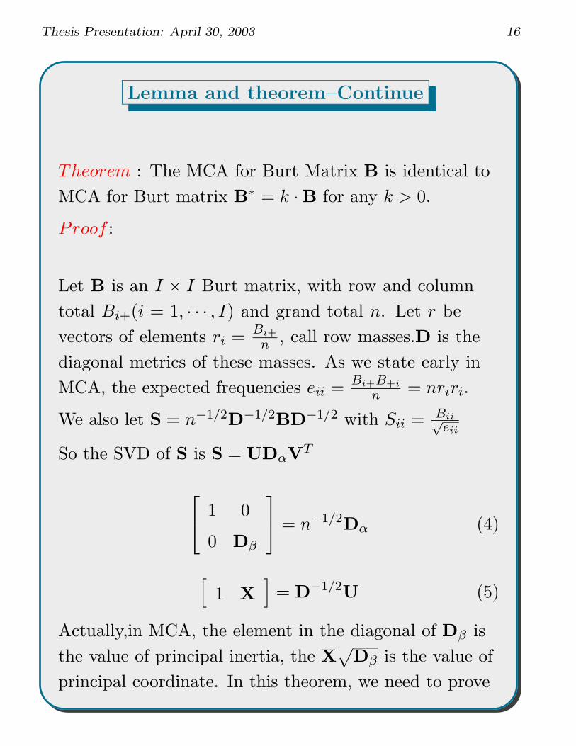
Lemma and theorem–Continue
Theorem : The MCA for Burt Matrix B is identical to
MCA for Burt matrix B∗ = k · B for any k > 0.
Proof :
Let B is an I × I Burt matrix, with row and column
total Bi+(i = 1, · · · , I) and grand total n. Let r be
vectors of elements ri = Bi+
n , call row masses.D is the
diagonal metrics of these masses. As we state early in
MCA, the expected frequencies eii = Bi+B+i
n = nriri.
We also let S = n−1/2D−1/2BD−1/2 with Sii = Bii√eii
So the SVD of S is S = UDαVT
1 0
0 Dβ
= n−1/2Dα (4)
[
1 X
]
= D−1/2
U (5)
Actually,in MCA, the element in the diagonal of Dβ is
the value of principal inertia, the X√
Dβ is the value of
principal coordinate. In this theorem, we need to prove
Page 17
Thesis Presentation: April 30, 2003 17
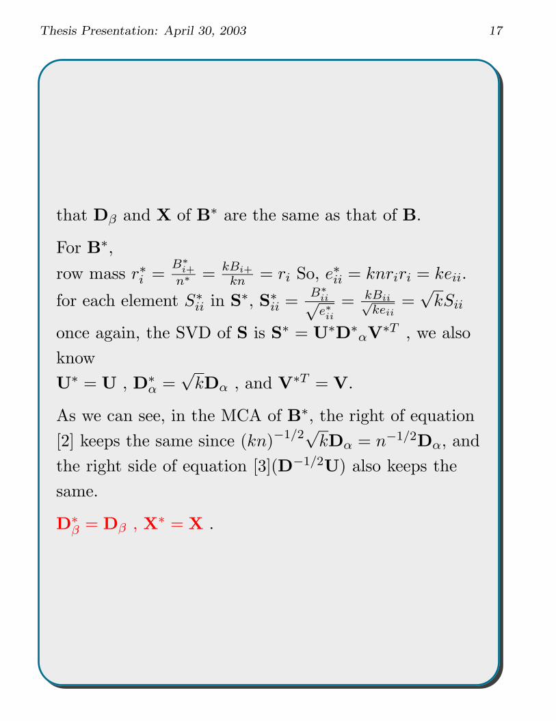
that Dβ and X of B∗ are the same as that of B.
For B∗,
row mass r∗i =B∗
i+
n∗ = kBi+
kn = ri So, e∗ii = knriri = keii.
for each element S∗ii in S∗, S∗
ii =B∗
ii√e∗ii
= kBii√keii
=√
kSii
once again, the SVD of S is S∗ = U∗D∗αV∗T , we also
know
U∗ = U , D∗α =
√kDα , and V∗T = V.
As we can see, in the MCA of B∗, the right of equation
[2] keeps the same since (kn)−1/2√
kDα = n−1/2Dα, and
the right side of equation [3](D−1/2U) also keeps the
same.
D∗β = Dβ , X∗ = X .
Page 18
Thesis Presentation: April 30, 2003 18
MSA Data
Brand1 Brand2 Male Female College High School
Brand1 695 0 373 322 499 196
Brand2 0 842 456 386 420 422
Male 373 456 829 0 457 372
Female 322 386 0 708 462 246
College 499 420 457 462 919 0
High School 196 422 372 246 0 618
Table 4: Burt Matrix
Brand1 Brand2 Male Female College High School
Brand1 346 349 373 322 499 196
Brand2 349 493 456 386 420 422
Male 373 456 468 361 457 372
Female 322 386 361 347 462 246
College 499 420 457 462 584 335
High School 196 422 372 246 335 283
Table 5: Modified Burt Matrix
Singular Principal Chi-Square Percent Cumulative
Value Inertia Percent Percent
Burt k=1 0.64473 0.41568 1993.5 41.57 41.57
matrix k=2 0.57628 0.33210 1592.67 33.21 74.78
k=3 0.50222 0.25233 1209.64 25.22 100.00
total 1 4795.81 100
Modified k=1 0.33318 0.11101 182.735 85.6 85.6
Burt k=2 0.13667 0.01868 30.749 14.4 100.00
Matrix total 0.12969 213.484 100
Table 6: Summary for MCA of Burt and Modified Burt Matrix
Page 19
Thesis Presentation: April 30, 2003 19
MSA Data-Continued
•
•
•
•
• •
First Principal Axis 41.57%
Seco
nd P
rincip
al Ax
is 33
.21%
-0.5 0.0 0.5 1.0
-0.5
0.00.5
1.0
Brand1
Brand2
Male
Female
College High School
MCA Graphical display of Burt Matrix for MSA Data
•
•
•
•
• •
First Principal Axis 85.6%
Seco
nd P
rincip
al Ax
is 14
.4%
-0.4 -0.2 0.0 0.2 0.4
-0.4
-0.2
0.00.2
0.4
Brand1
Brand2
Male
Female
College High School
MCA Graphical display of Modified Burt Matrix for MSA Data
Page 20
Thesis Presentation: April 30, 2003 20
Conclusion and Future Work
Identify the characteristics of data that work well with
Greenacre method.
Page 21
Thesis Presentation: April 30, 2003 21
Reference
Beh, E.J. (1997). Simple correspondence analysis of ordinal
cross-classifications using orthogonal polynomials. Biometrical Journal,
39, 589-613.
Bendixen, M (1996). A practical guide to the use of correspondence
analysis in marketing research. Marketing Research on-line Vol 1.
Greenacre,M.J. (1984). Theory and Applications of Correspondence
Analysis. London: Academic Press.
Greenacre, M.J. (1988). Correspondence Analysis of Multivariate
categorical data by weighted least squares. Biometrika, 75, 457-467.
Greenacre, M.J. and Balasius, J. (1994). Correspondence Analysis in the
Social Sciences. London: Academic Press.
Hoffman, D.L.and Franke,G.R (1986). Correspondence Analysis:
Graphical Representation of Categorical Data in Marketing Research.
Journal of Marketing Research, Vol 23:3,213-227.
Page 22
Thesis Presentation: April 30, 2003 22
S − Plus Code
Function to calculate the Square Root of Matrix A
pdsroot <- function(A)
{
p <- dim(A)[1] # dimension of matrix
eigenv <- eigen(A, symmetric = T) # spectral decomposition of A
rootA <- eigenv$vectors %*% diag(sqrt(eigenv$values)) %*% t(eigenv$vectors)
rootA
}
Perform MCA for Burt matrix in S-plus
r_apply(N,1,sum) # N is the i by i Burt Matrix
n_sum(r)
r_apply(N,1,sum)/n
c_apply(N,2,sum)/n
Dr_diag(r)
Dc_diag(c)
S_(1/sqrt(n))*solve(pdsroot(Dr))%*%N%*%solve(pdsroot(Dc))
U_svd(S)$u
V_svd(S)$v
Dalph<-diag(svd(S)$d)
Dmu_(sqrt(1/n)*Dalph)[2:(i-1),2:(i-1)] # Dmu is the principal inertia
X_pdsroot(Dr) #sqrt(Dmu) is the singular value
X_solve(X)%*%U
X_X/X[1,1]
X_X[1:(i-1),2:(i-1)]
Y_pdsroot(Dc)
Y_solve(Y)%*%V
Y_Y/Y[1,1]
Y_Y[1:(i-1),2:(i-1)]
dyc_n*(r%*%t(c)+Dr%*%X%*%Dmu%*%t(Y)%*%Dc) # dyc is the Weight
# least-squares approximation of Burt matrix
fs<-X%*%sqrt(Dmu) # this is the principal coordinate
#for row and column ( note: row and column is same in this case)
Page 23
Thesis Presentation: April 30, 2003 23
S-Plus Code-Continue
Iterative Alogrithm to obtain the Modified Burt Matrix for MSA Data (number of
observation is 1537), B is 6 by 6 Burt Matrix, and have three categorical variables,
each has 2 variables.
N<-B
for (i in 1:5)
{
r_apply(N,1,sum)
n_sum(r)
r_apply(N,1,sum)/n
c_apply(N,2,sum)/n
Dr_diag(r)
Dc_diag(c)
S_(1/sqrt(n))*solve(pdsroot(Dr))%*%N%*%solve(pdsroot(Dc))
U_svd(S)$u
V_svd(S)$v
Dalph<-diag(svd(S)$d)
Dmu_(sqrt(1/n)*Dalph)[2:6,2:6]
X_pdsroot(Dr)
X_solve(X)%*%U
X_X/X[1,1]
X_X[1:6,2:6]
Y_pdsroot(Dc)
Y_solve(Y)%*%V
Y_Y/Y[1,1]
Y_Y[1:6,2:6]
dyc_n*(r%*%t(c)+Dr%*%X%*%Dmu%*%t(Y)%*%Dc)
Dbeta<-sqrt(Dmu)
N<-B
N11<-N[1:2,1:2]
R11<-apply(N11,1,sum)
D11<-diag(R11)
X11<-X[1:2,1:5]
N11star<-round(R11%*%t(R11)/1537)
N11star<-N11star+round(D11%*%X11%*%Dbeta%*%t(X11)%*%D11/n)
N22<-N[3:4,3:4]
R22<-apply(N22,1,sum)
D22<-diag(R22)
Page 24
Thesis Presentation: April 30, 2003 24
X22<-X[3:4,1:5]
N22star<-round(R22%*%t(R22)/1537)
N22star<-N22star+round(D22%*%X22%*%Dbeta%*%t(X22)%*%D22/n)
N33<-N[5:6,5:6]
R33<-apply(N33,1,sum)
D33<-diag(R33)
X33<-X[5:6,1:5]
N33star<-round(R33%*%t(R33)/1537)
N33star<-N33star+round(D33%*%X33%*%Dbeta%*%t(X33)%*%D33/n)
N[1:2,1:2]<-N11star
N[3:4,3:4]<-N22star
N[5:6,5:6]<-N33star
}
Plot two-dimensional graphical display
fsname<-c(’Brand1’,’Brand2’,’Male’,’Female’,’College’,’High School’)
corrplot<-function(fs,fsname)
{
xlabes<-fsname
plot(fs[,1],fs[,2],pch="*",xlim=range(fs),ylim=range(fs),xlab=paste("First
Principal Axis "),ylab=paste("Second Principal Axis"))
text(dycfs[,1]-0.01,dycfs[,2]-0.03,labels=xlabes,adj=0)
title(main="MCA Graphical display of Modified Burt Matrix for MSA Data")
abline(h=0,v=0)
return(fs=fs[,c(1,2)])
}