1 1 Multiple Linear Regression Multiple Linear Regression Multiple Linear Regression Multiple Linear Regression by Lin Naing @ Mohd. Lin Naing @ Mohd. Lin Naing @ Mohd. Lin Naing @ Mohd. Ayub Ayub Ayub Ayub Sadiq Sadiq Sadiq Sadiq School of Dental Sciences School of Dental Sciences School of Dental Sciences School of Dental Sciences Universiti Sains Malaysia Universiti Sains Malaysia Universiti Sains Malaysia Universiti Sains Malaysia
Transcript
1
1
Multiple Linear RegressionMultiple Linear RegressionMultiple Linear RegressionMultiple Linear Regression
by
Lin Naing @ Mohd. Lin Naing @ Mohd. Lin Naing @ Mohd. Lin Naing @ Mohd. AyubAyubAyubAyub SadiqSadiqSadiqSadiq
School of Dental SciencesSchool of Dental SciencesSchool of Dental SciencesSchool of Dental Sciences
Universiti Sains MalaysiaUniversiti Sains MalaysiaUniversiti Sains MalaysiaUniversiti Sains Malaysia
2
2
ContentsContentsContentsContents
Simple Linear Regression (Revision)Simple Linear Regression (Revision)Simple Linear Regression (Revision)Simple Linear Regression (Revision)
Basic Theory of Multiple Linear RegressionBasic Theory of Multiple Linear RegressionBasic Theory of Multiple Linear RegressionBasic Theory of Multiple Linear Regression
Steps in Handling Multiple Linear Regression AnalysisSteps in Handling Multiple Linear Regression AnalysisSteps in Handling Multiple Linear Regression AnalysisSteps in Handling Multiple Linear Regression Analysis
Data Presentation and InterpretationData Presentation and InterpretationData Presentation and InterpretationData Presentation and Interpretation
3
3
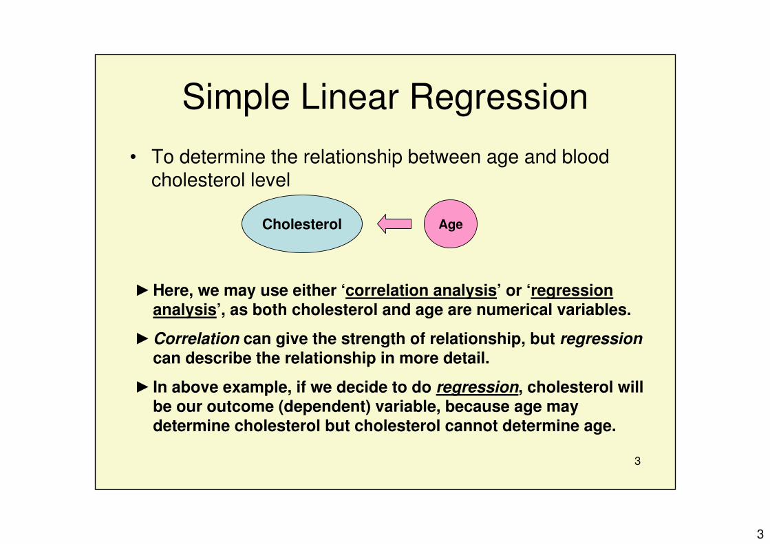
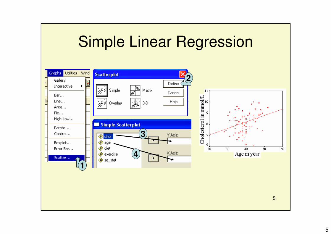
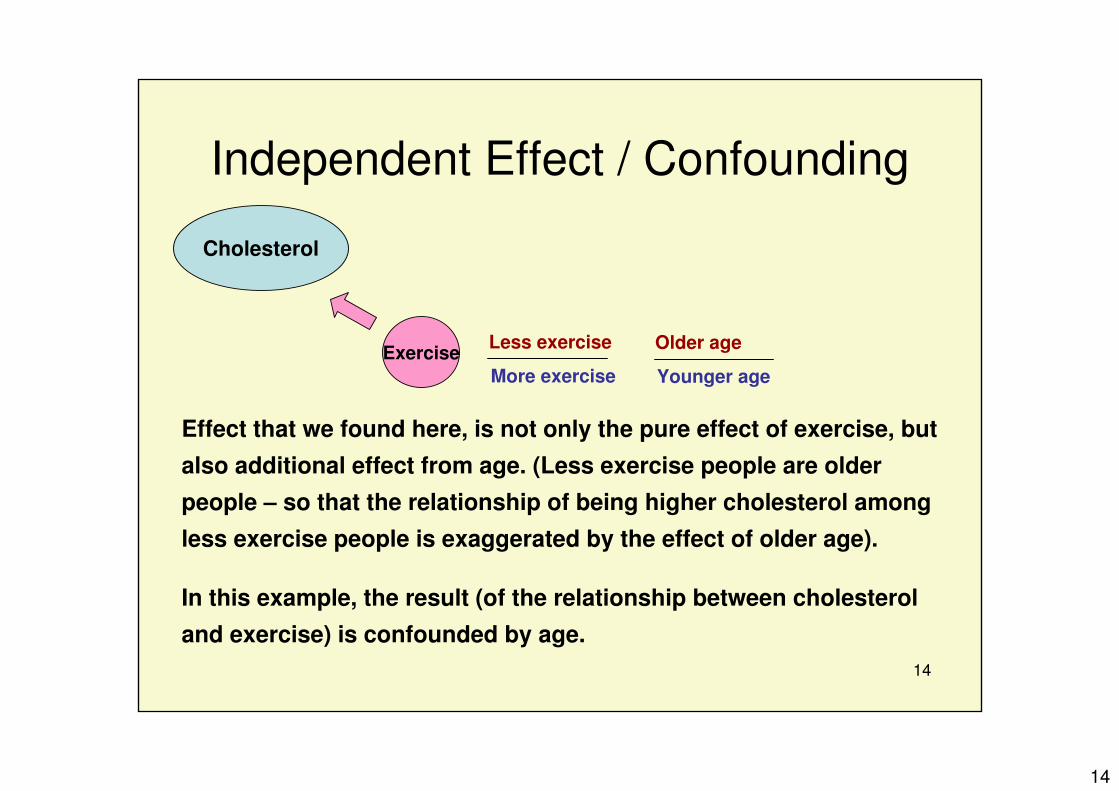
►Here, we may use either ‘correlation analysis’ or ‘regression analysis’, as both cholesterol and age are numerical variables.
►Correlation can give the strength of relationship, but regression
can describe the relationship in more detail.
► In above example, if we decide to do regression, cholesterol will be our outcome (dependent) variable, because age may
determine cholesterol but cholesterol cannot determine age.
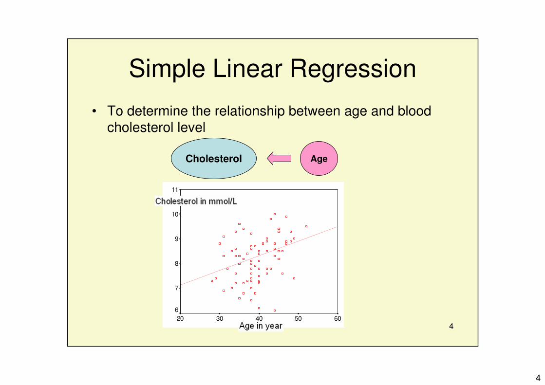
• To determine the relationship between age and blood cholesterol level
Cholesterol Age
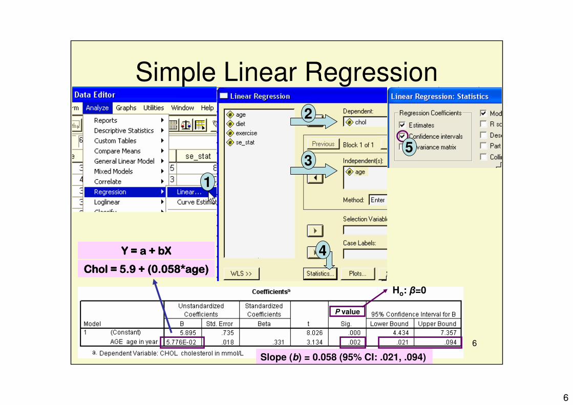
Simple Linear Regression
4
4
• To determine the relationship between age and blood cholesterol level
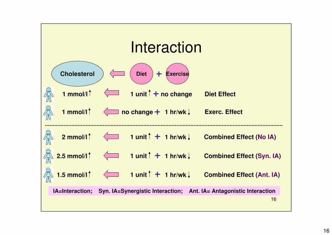
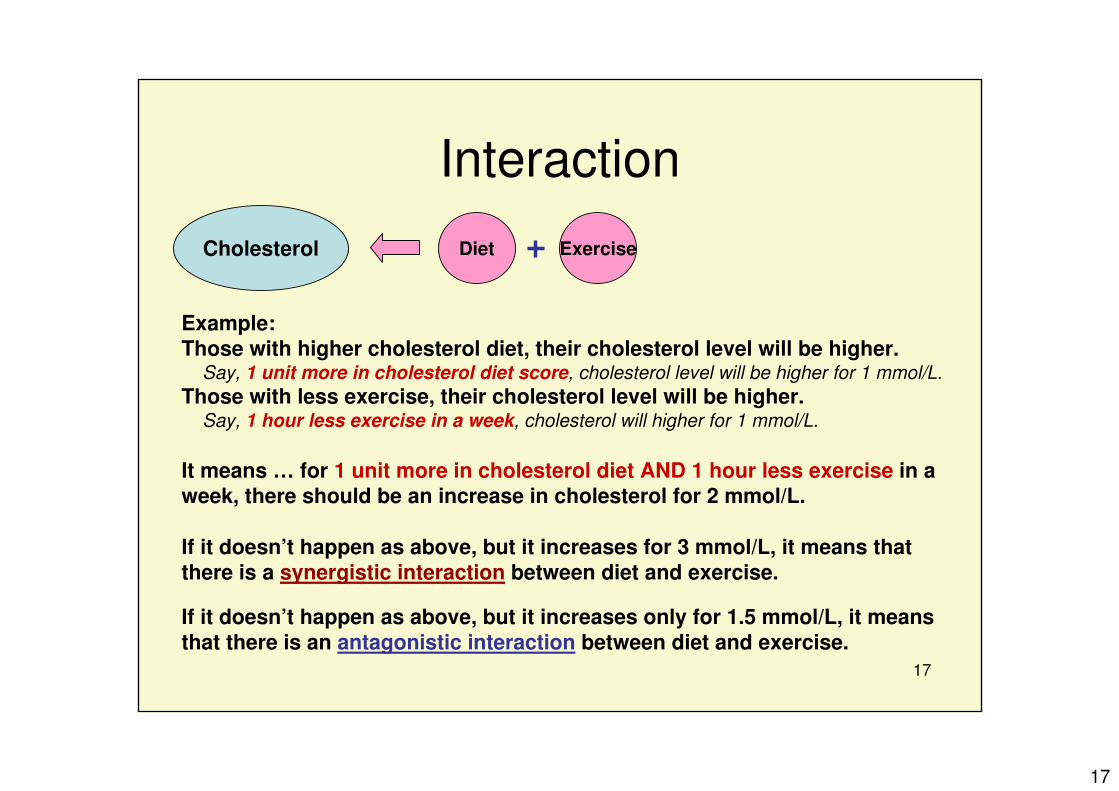
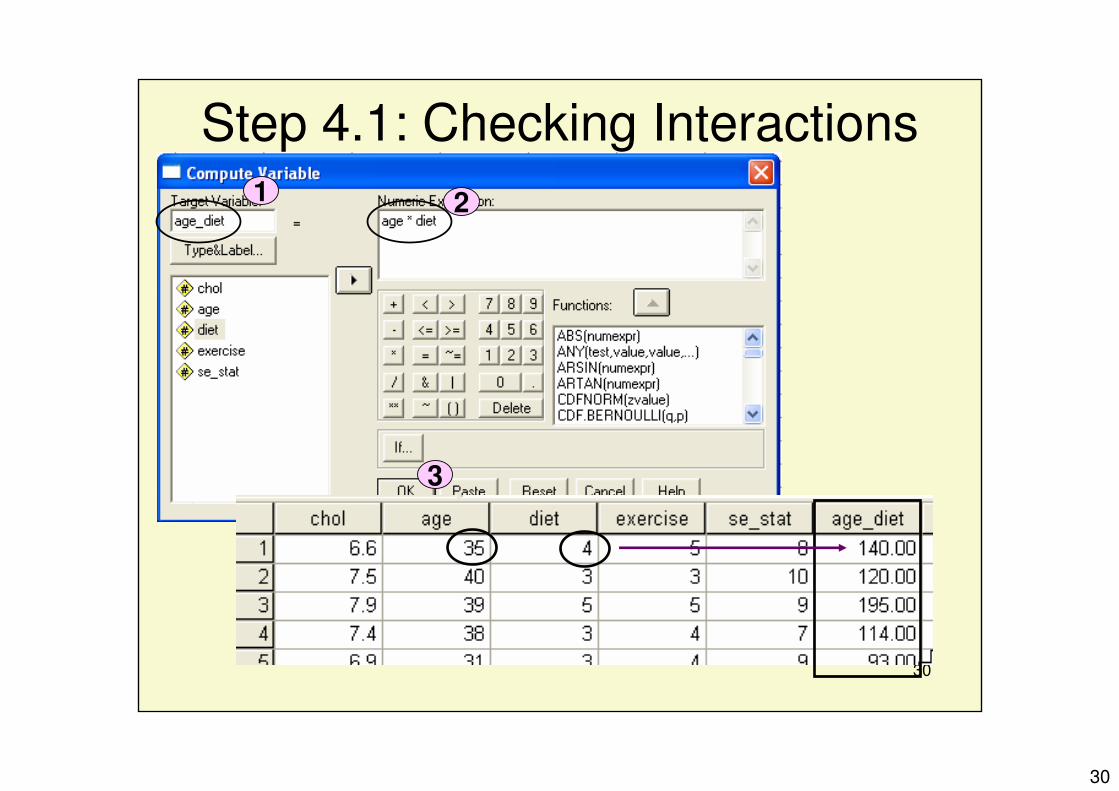
Those with higher cholesterol diet, their cholesterol level will be higher.Say, 1 unit more in cholesterol diet score, cholesterol level will be higher for 1 mmol/L.
Those with less exercise, their cholesterol level will be higher.Say, 1 hour less exercise in a week, cholesterol will higher for 1 mmol/L.
It means … for 1 unit more in cholesterol diet AND 1 hour less exercise in a
week, there should be an increase in cholesterol for 2 mmol/L.
If it doesn’t happen as above, but it increases for 3 mmol/L, it means that
there is a synergistic interaction between diet and exercise.
If it doesn’t happen as above, but it increases only for 1.5 mmol/L, it means
that there is an antagonistic interaction between diet and exercise.
18
18
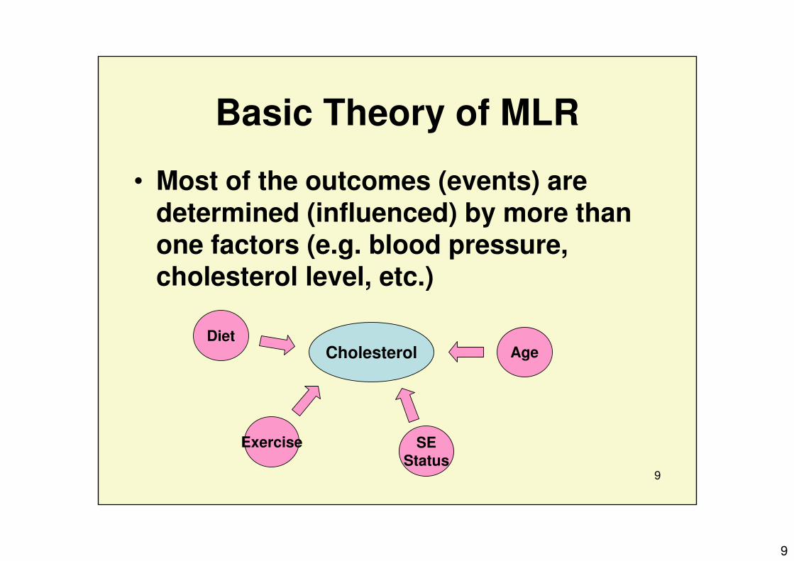
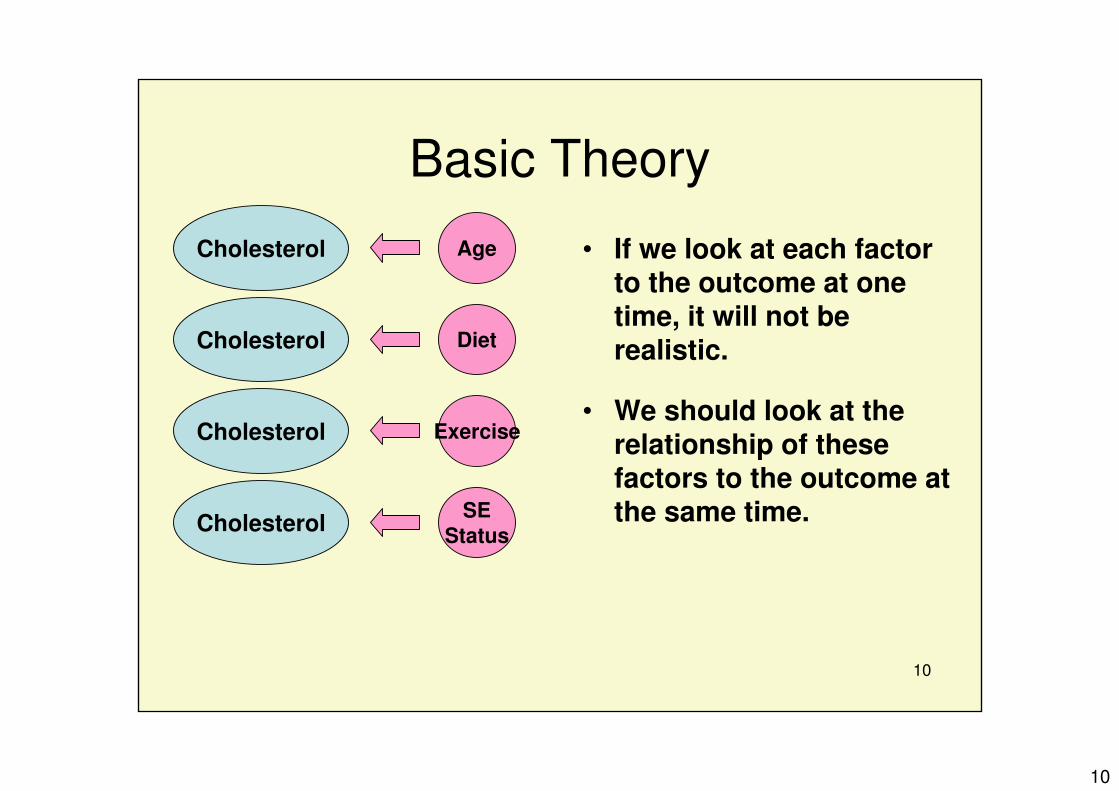
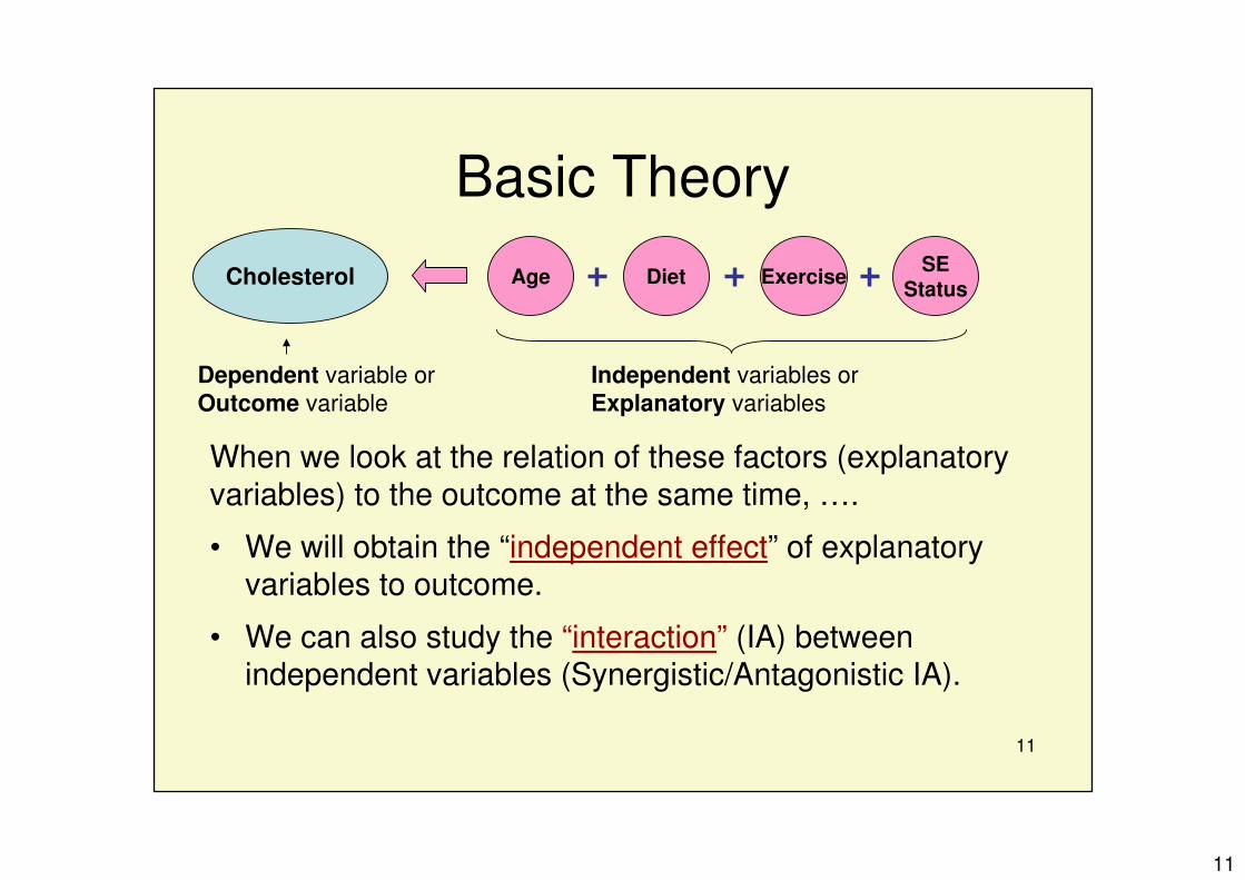
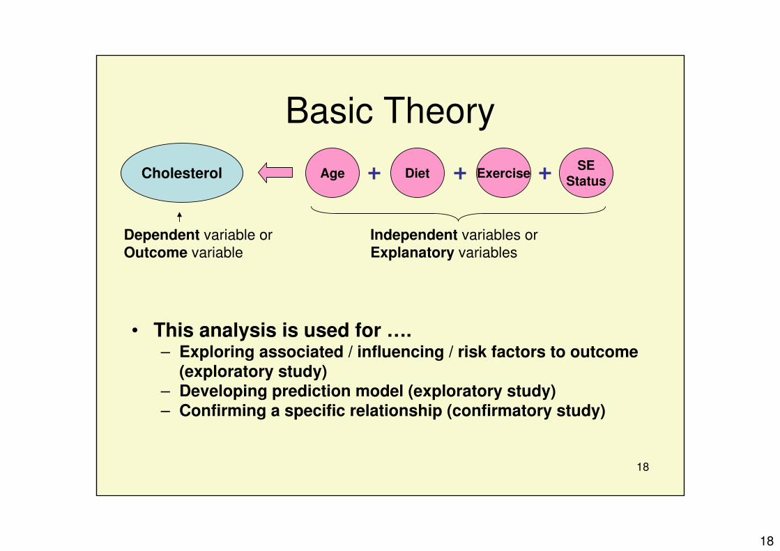
Basic Theory
Cholesterol Age Diet ExerciseSE
Status
Independent variables or
Explanatory variables
Dependent variable or
Outcome variable
• This analysis is used for ….– Exploring associated / influencing / risk factors to outcome
(exploratory study)– Developing prediction model (exploratory study)
– Confirming a specific relationship (confirmatory study)
19
19
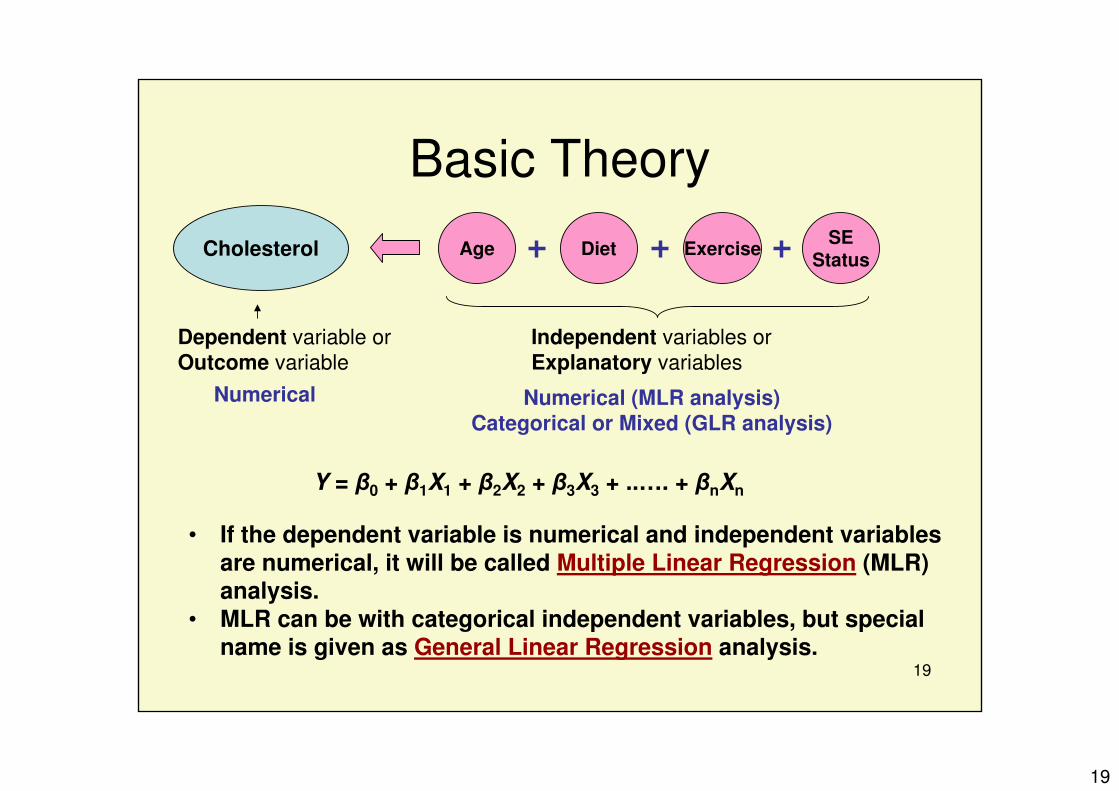
Basic Theory
• If the dependent variable is numerical and independent variables
are numerical, it will be called Multiple Linear Regression (MLR) analysis.
• MLR can be with categorical independent variables, but special name is given as General Linear Regression analysis.
Cholesterol Age Diet ExerciseSE
Status
Dependent variable or
Outcome variable
Numerical Numerical (MLR analysis)
Categorical or Mixed (GLR analysis)
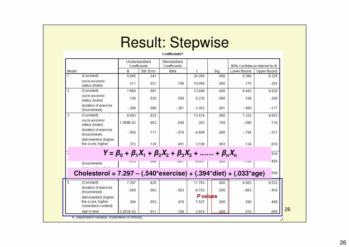
Y = β0 + β1X1 + β2X2 + β3X3 + ..…. + βnXn
Independent variables or
Explanatory variables
20
20
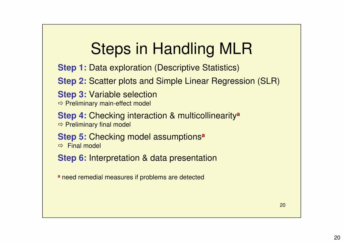
Steps in Handling MLRStep 1: Data exploration (Descriptive Statistics)
Step 2: Scatter plots and Simple Linear Regression (SLR)
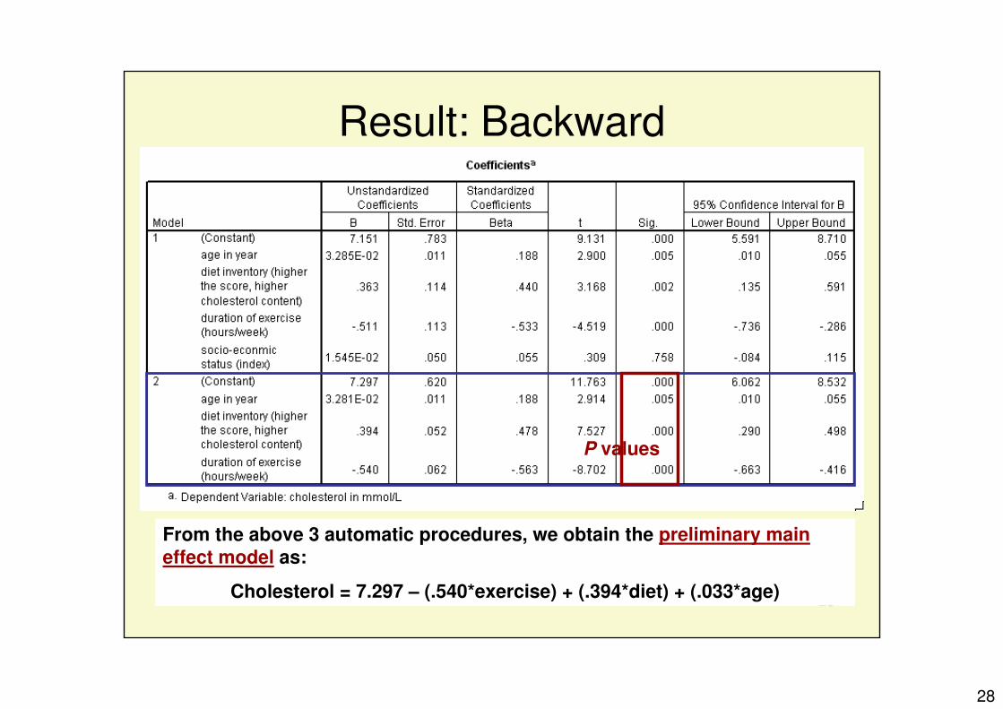
Step 3: Variable selection� Preliminary main-effect model
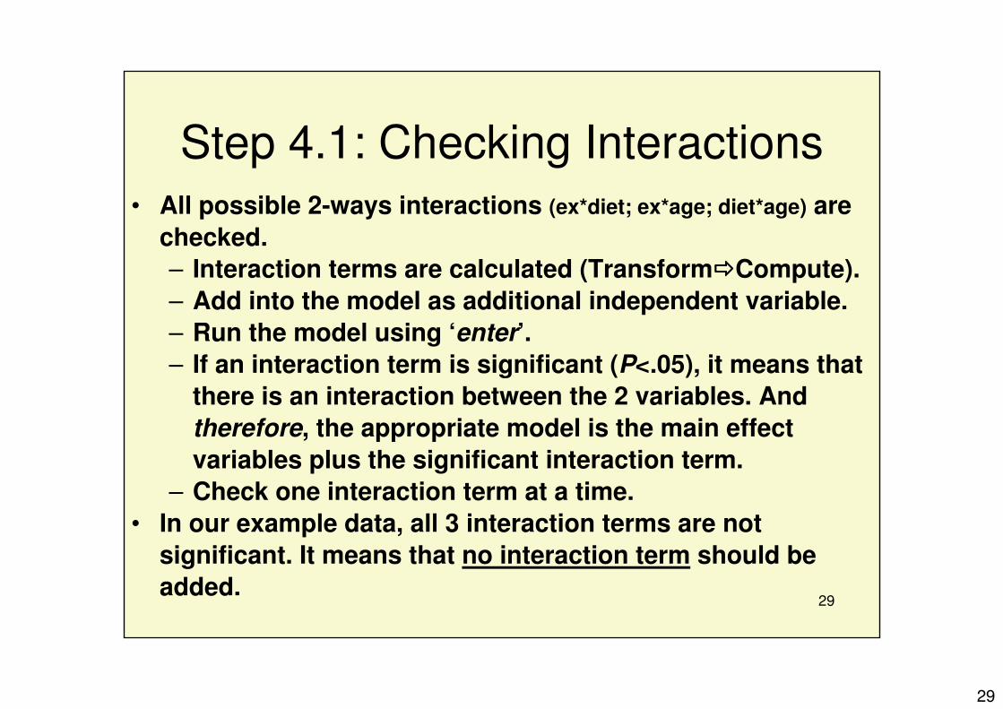
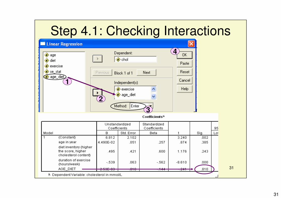
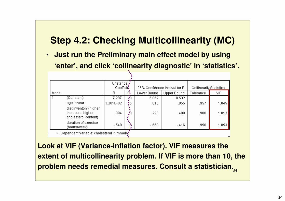
Step 4: Checking interaction & multicollinearitya
� Preliminary final model
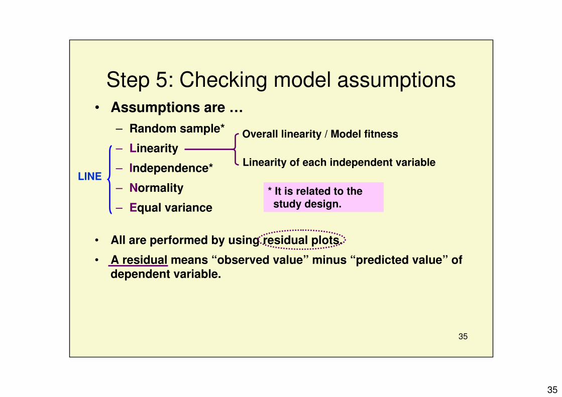
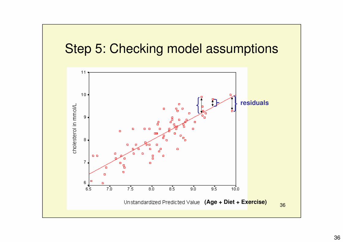
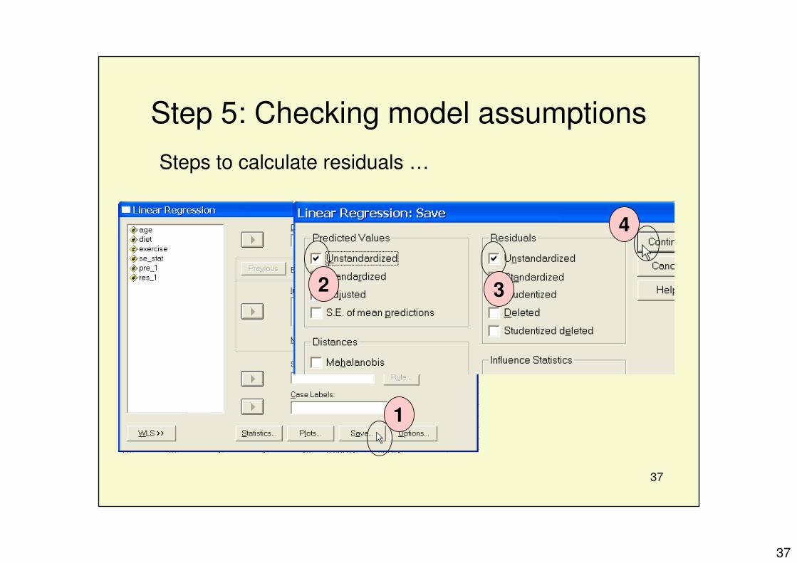
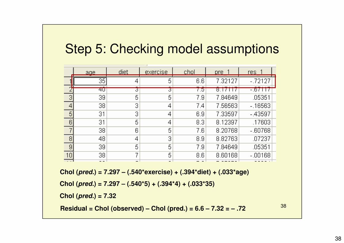
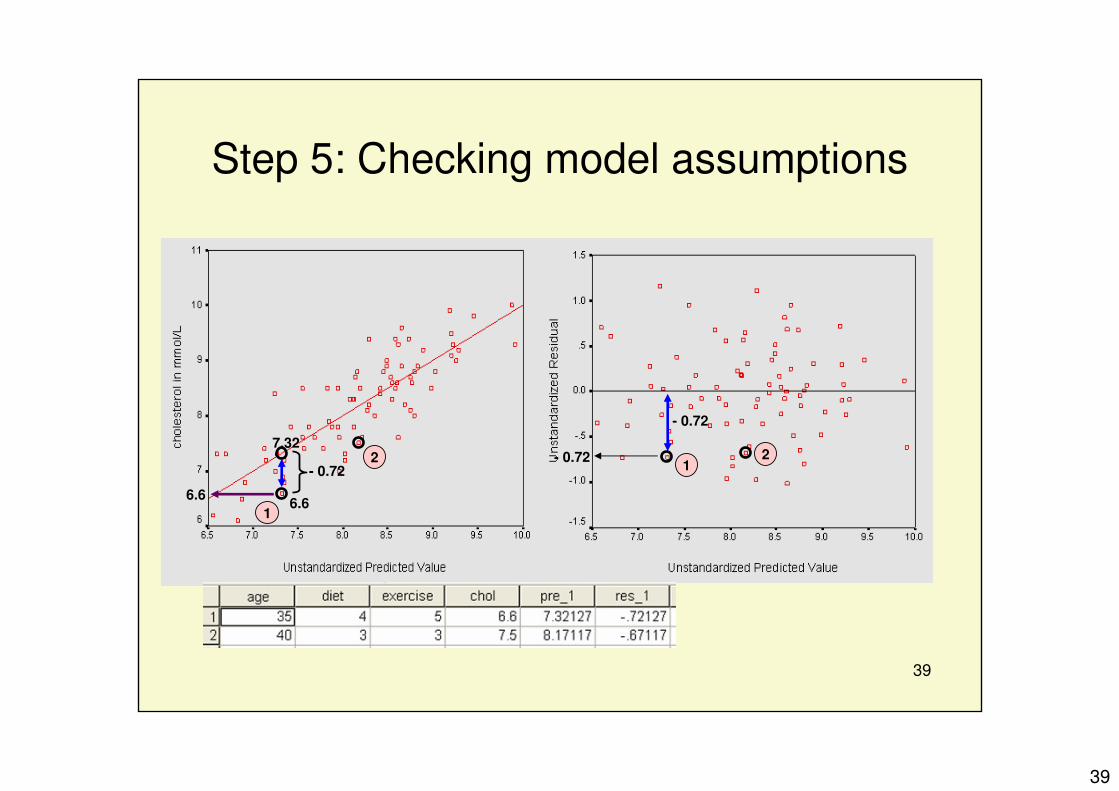
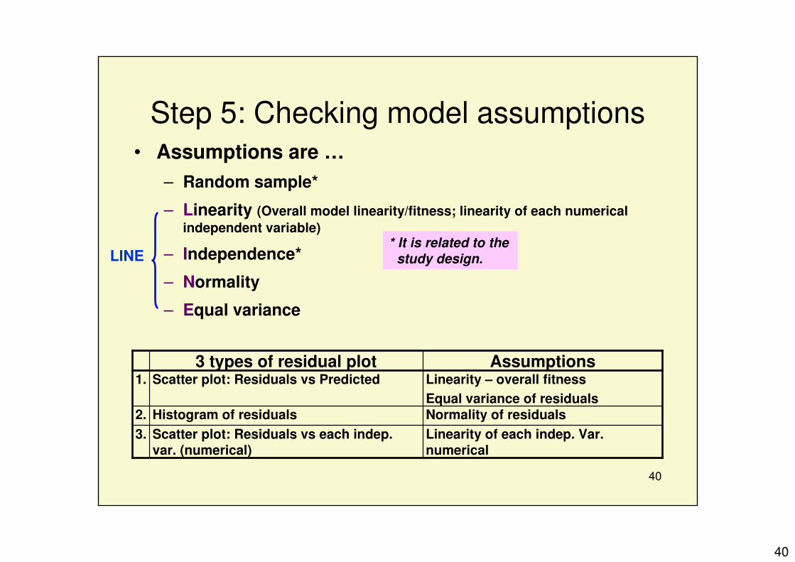
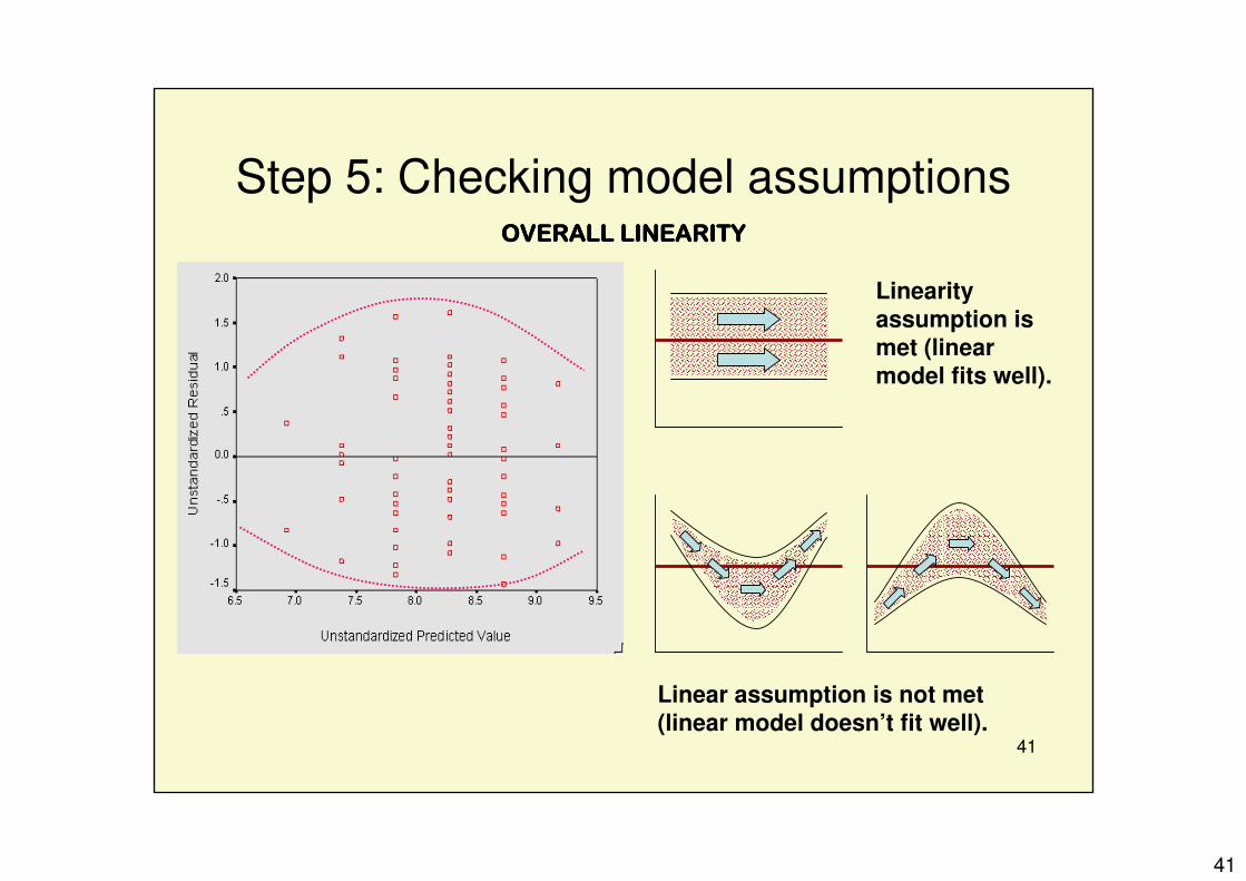
Step 5: Checking model assumptionsa
� Final model
Step 6: Interpretation & data presentation
a need remedial measures if problems are detected
21
21
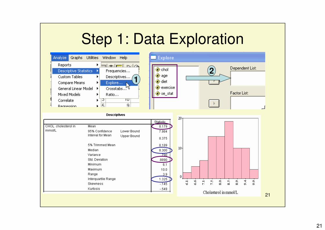
Step 1: Data Exploration
12
22
22
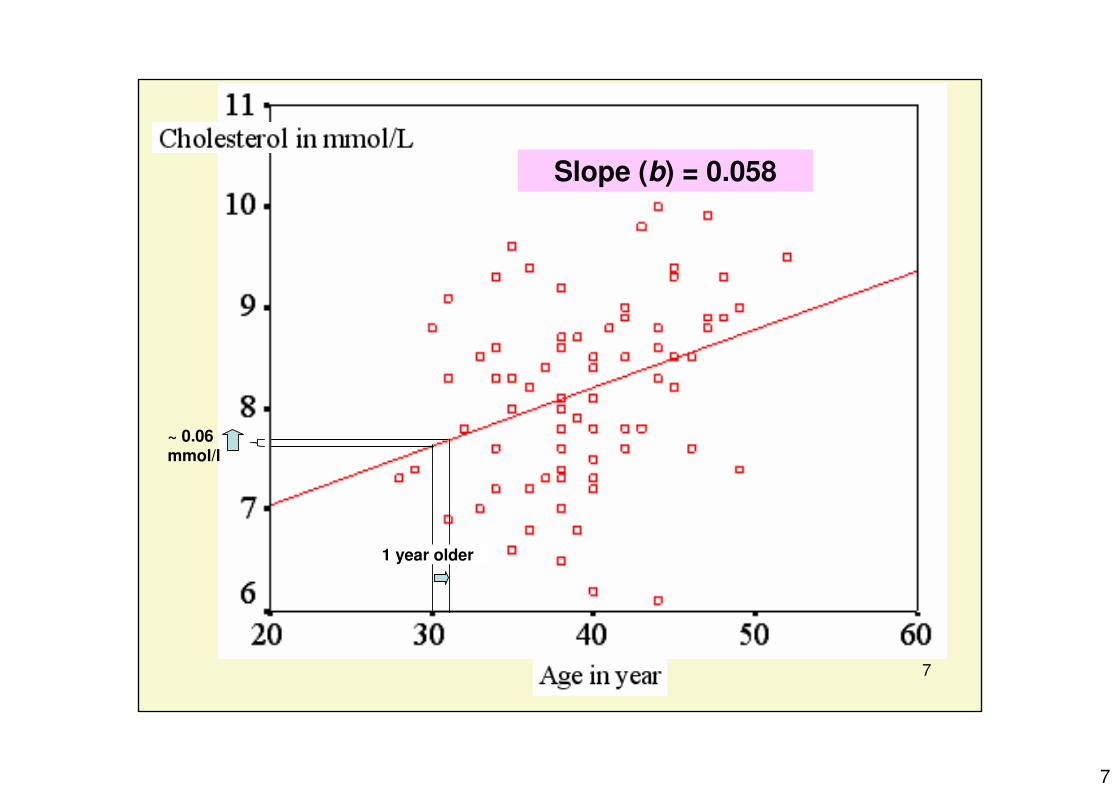
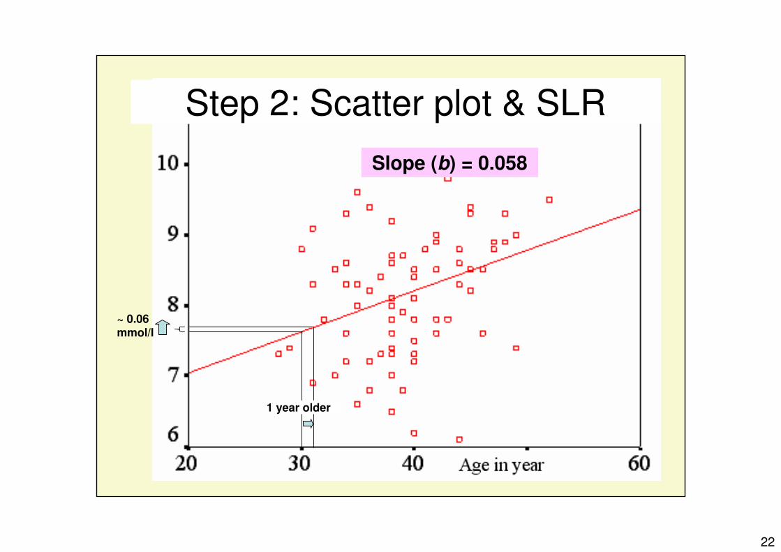
1 year older
~ 0.06mmol/l
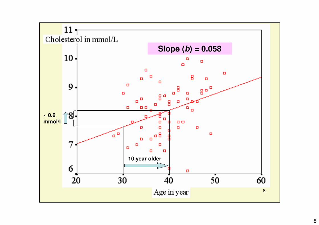
Slope (b) = 0.058
Step 2: Scatter plot & SLR
23
23
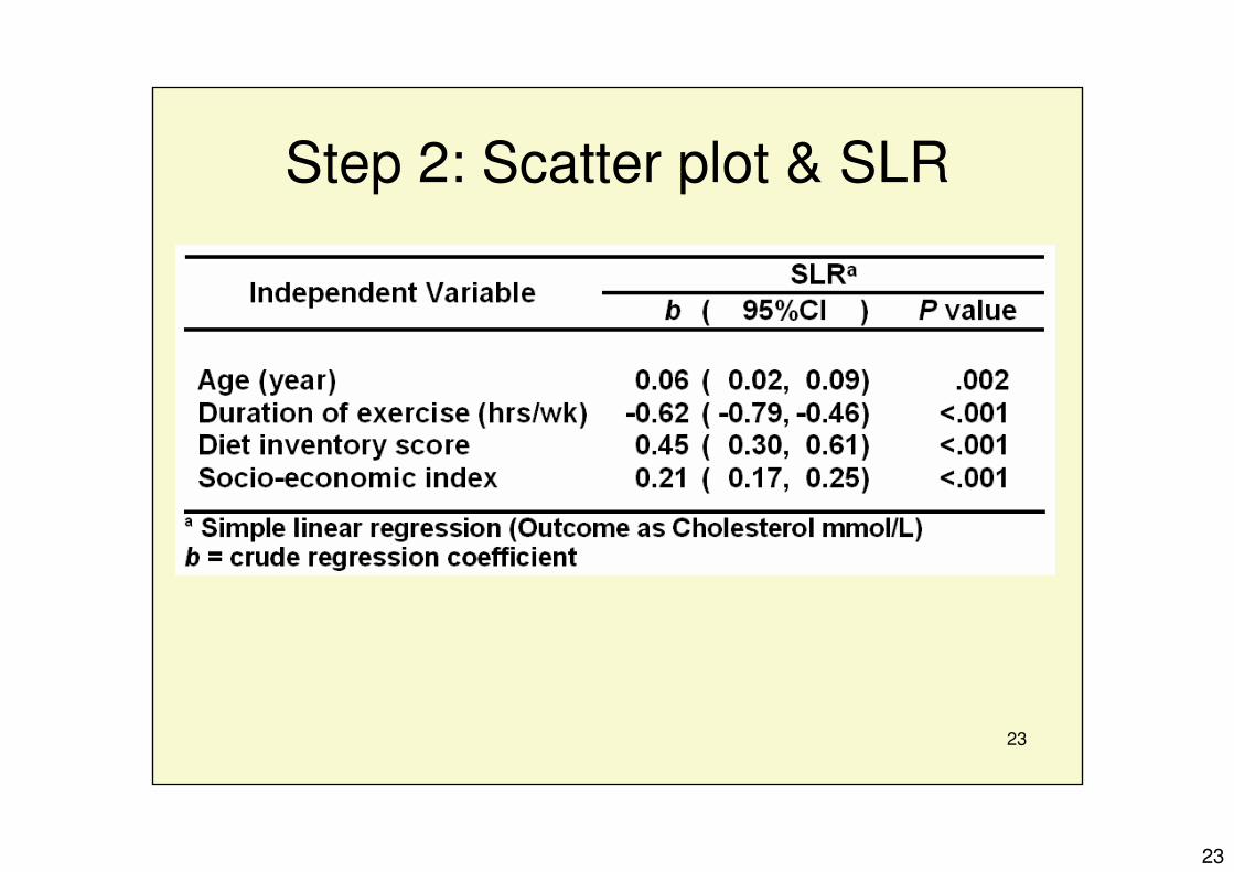
Step 2: Scatter plot & SLR
24
24
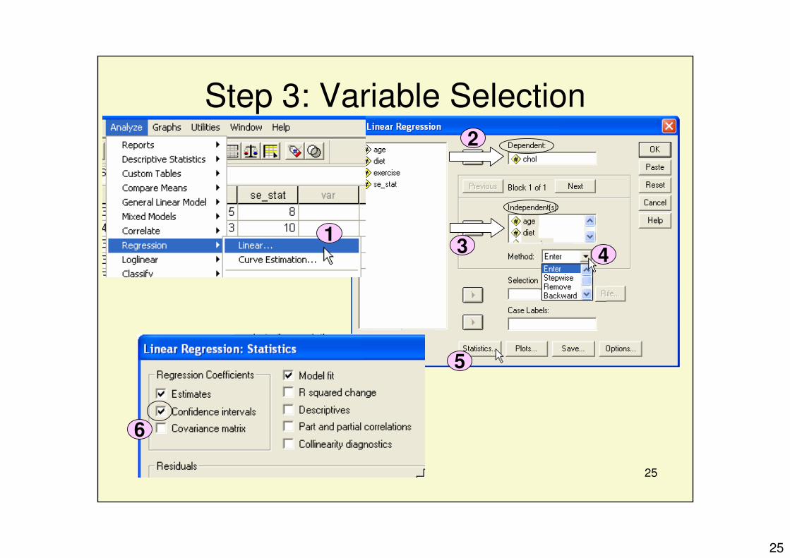
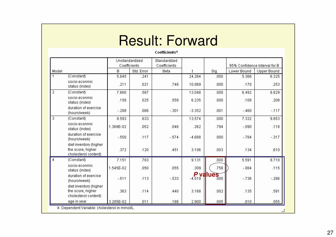
Step 3: Variable Selection
• Automatic / Manual methods
– Forward method
– Backward method
– Stepwise method
– All possible models method
• Nowadays, as computers are faster, automatic
methods can be done easily.
• In SPSS, forward, backward and stepwise can be
used.
• All 3 methods should be used for this step. Take the
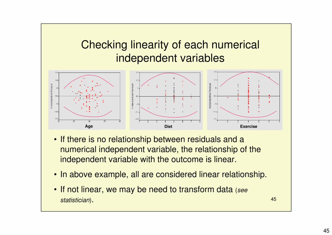
• If there is no relationship between residuals and a numerical independent variable, the relationship of the independent variable with the outcome is linear.
• In above example, all are considered linear relationship.
• If not linear, we may be need to transform data (see
statistician).
Age Diet Exercise
Checking linearity of each numerical
independent variables
46
46
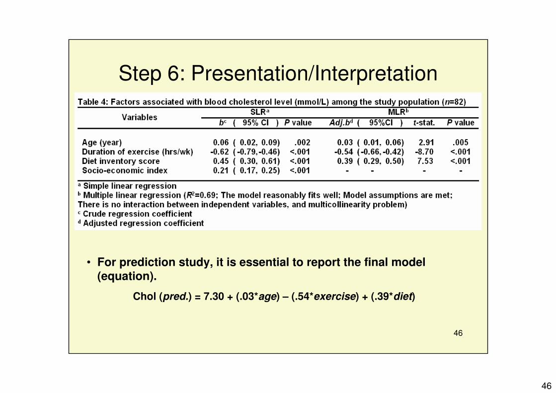
Step 6: Presentation/Interpretation
• For prediction study, it is essential to report the final model (equation).
• There is a significant linear relationship between age and cholesterol
level (P=.005). Those with 10 years older have cholesterol level higher
for 0.3 mmol/L (95% CI: 0.1, 0.6 mmol/L).
• There is a significant linear relationship between duration of exercise
and cholesterol level (P<.001). Those having 1 hr/wk less exercise
have cholesterol level higher for 0.54 mmol/L (95% CI: 0.66, 0.42
mmol/L).
• There is a significant linear relationship between diet inventory index
and cholesterol level (P<.001). Those with 1 unit more in the index,
have cholesterol level higher for 0.39 mmol/L (95% CI: 0.29, 0.50
mmol/L).
• With the 3 significant variables, the model explains 69% of variation
of the blood cholesterol level in the study sample. (R2=0.69)
48
48
Categorical Independent Var.Cautions:It should be coded (0, 1) for dichotomous variable.
Example 1: sex (male=1, female=0)It means we are comparing male against female (female as reference)
Example 2: smoking (smokers=1, non-smoker=0)It means we are comparing smokers against non-smoker (non-smoker as reference)
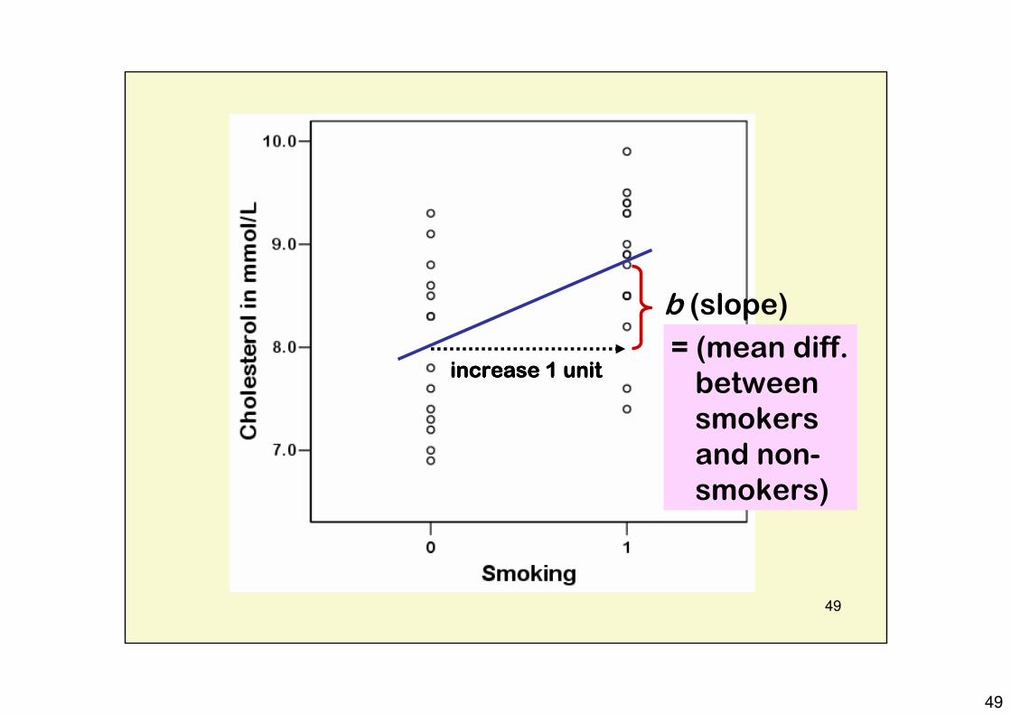
Say, outcome is cholesterol, smoking as independent var., and we got b=2.0. It means smokers will have cholesterol level higher than non-smokers for 2.0 mmol/L.
49
49
b (slope)
= (mean diff. between smokers and non-smokers)
increase 1 unitincrease 1 unitincrease 1 unitincrease 1 unit
50
50
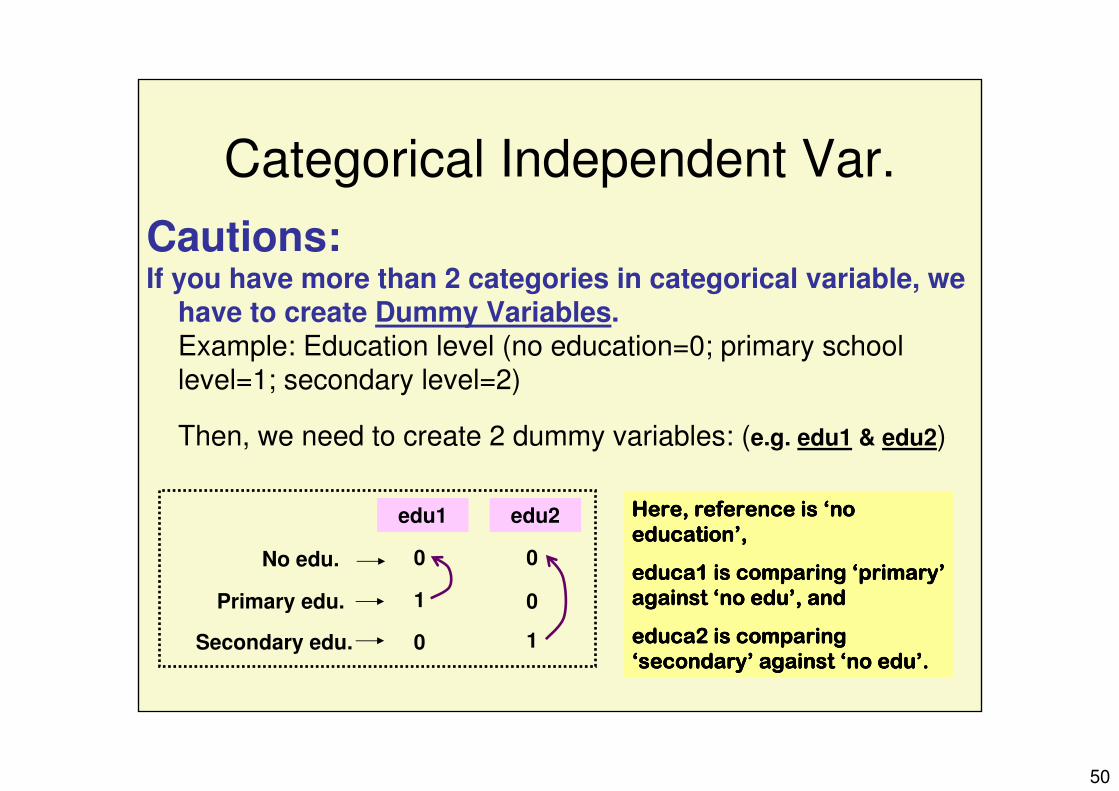
Categorical Independent Var.
Cautions:If you have more than 2 categories in categorical variable, we
have to create Dummy Variables. Example: Education level (no education=0; primary school level=1; secondary level=2)
Then, we need to create 2 dummy variables: (e.g. edu1 & edu2)
edu1 edu2
No edu.
Primary edu.
Secondary edu.
0 0
1 0
10
Here, reference is Here, reference is Here, reference is Here, reference is ‘‘‘‘no no no no educationeducationeducationeducation’’’’,,,,
educa1 is comparing educa1 is comparing educa1 is comparing educa1 is comparing ‘‘‘‘primaryprimaryprimaryprimary’’’’against against against against ‘‘‘‘no no no no eduedueduedu’’’’, and, and, and, and
educa2 is comparing educa2 is comparing educa2 is comparing educa2 is comparing ‘‘‘‘secondarysecondarysecondarysecondary’’’’ against against against against ‘‘‘‘no no no no eduedueduedu’’’’....
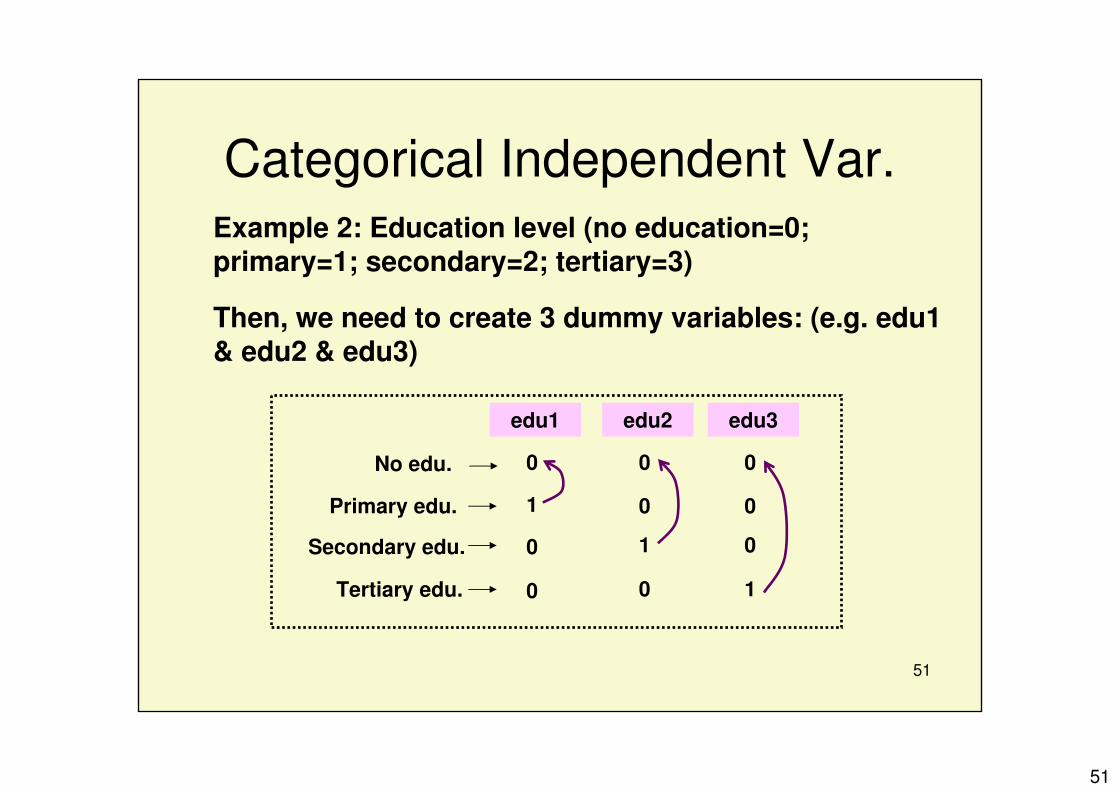
Then, we need to create 3 dummy variables: (e.g. edu1 & edu2 & edu3)
edu1 edu2
No edu.
Primary edu.
Secondary edu.
0 0
1 0
10
edu3
0
0
0
Tertiary edu. 00 1
52
52
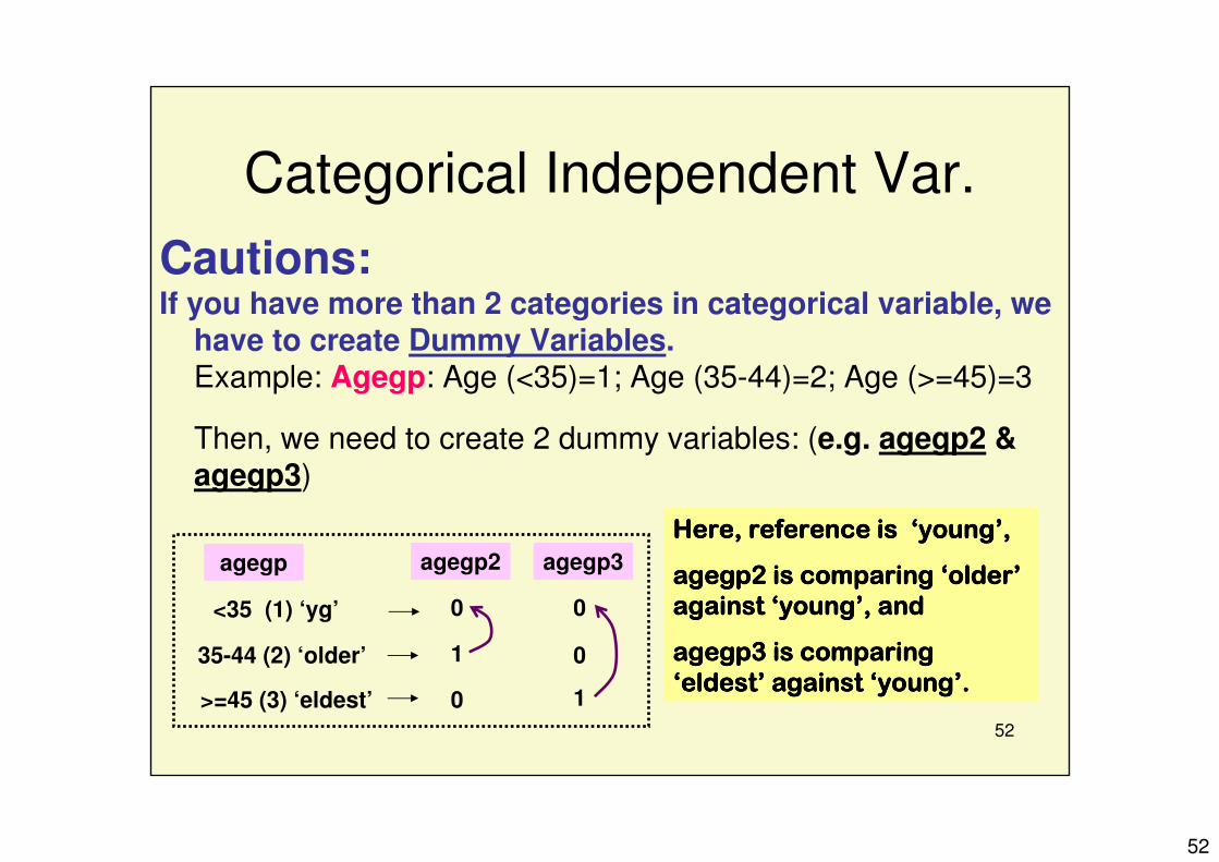
Categorical Independent Var.
Cautions:If you have more than 2 categories in categorical variable, we
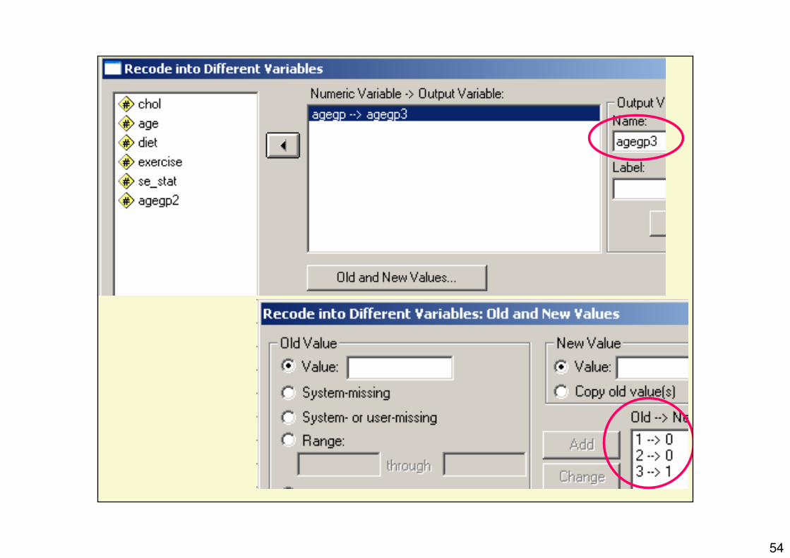
have to create Dummy Variables. Example: Agegp: Age (<35)=1; Age (35-44)=2; Age (>=45)=3
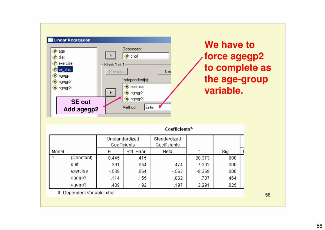
Then, we need to create 2 dummy variables: (e.g. agegp2 & agegp3)
agegp2 agegp3
<35 (1) ‘yg’
35-44 (2) ‘older’
>=45 (3) ‘eldest’
0 0
1 0
10
Here, reference is Here, reference is Here, reference is Here, reference is ‘‘‘‘youngyoungyoungyoung’’’’,,,,
agegp2 is comparing agegp2 is comparing agegp2 is comparing agegp2 is comparing ‘‘‘‘olderolderolderolder’’’’against against against against ‘‘‘‘youngyoungyoungyoung’’’’, and, and, and, and
agegp3 is comparing agegp3 is comparing agegp3 is comparing agegp3 is comparing ‘‘‘‘eldesteldesteldesteldest’’’’ against against against against ‘‘‘‘youngyoungyoungyoung’’’’....
agegp
53
53
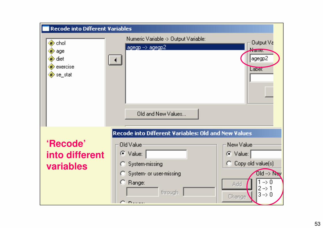
‘Recode’
into different
variables
54
54
55
55
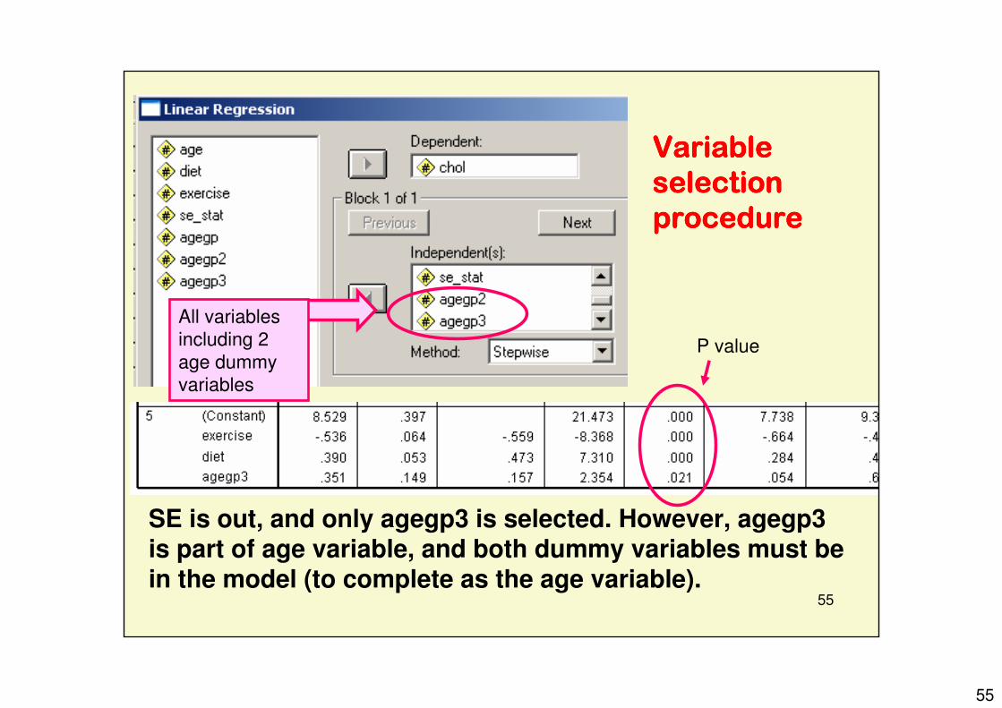
SE is out, and only agegp3 is selected. However, agegp3 is part of age variable, and both dummy variables must be in the model (to complete as the age variable).
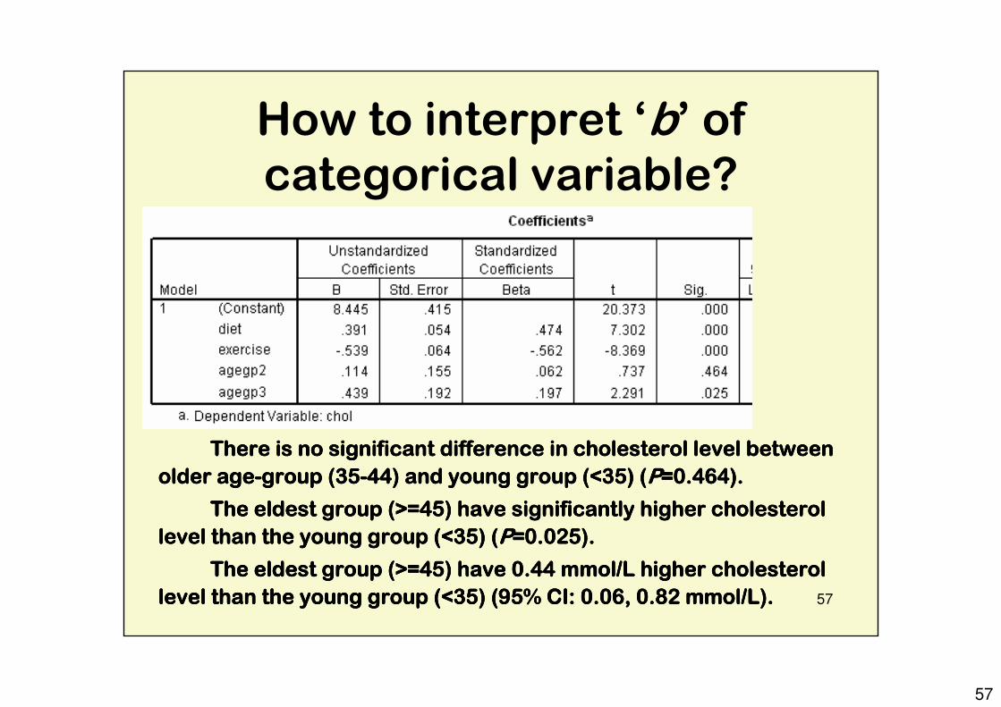
There is no significant difference in cholesterol level between There is no significant difference in cholesterol level between There is no significant difference in cholesterol level between There is no significant difference in cholesterol level between
older ageolder ageolder ageolder age----group (35group (35group (35group (35----44) and young group (<35) (44) and young group (<35) (44) and young group (<35) (44) and young group (<35) (PPPP=0.464).=0.464).=0.464).=0.464).
The eldest group (>=45) have significantly higher cholesterol The eldest group (>=45) have significantly higher cholesterol The eldest group (>=45) have significantly higher cholesterol The eldest group (>=45) have significantly higher cholesterol
level than the young group (<35) (level than the young group (<35) (level than the young group (<35) (level than the young group (<35) (PPPP=0.025).=0.025).=0.025).=0.025).
The eldest group (>=45) have 0.44 The eldest group (>=45) have 0.44 The eldest group (>=45) have 0.44 The eldest group (>=45) have 0.44 mmolmmolmmolmmol/L higher cholesterol /L higher cholesterol /L higher cholesterol /L higher cholesterol
level than the young group (<35) (95% CI: 0.06, 0.82 level than the young group (<35) (95% CI: 0.06, 0.82 level than the young group (<35) (95% CI: 0.06, 0.82 level than the young group (<35) (95% CI: 0.06, 0.82 mmolmmolmmolmmol/L)./L)./L)./L).