Department of Computer Science and Engineering University of Texas at Arlington Arlington, TX 76019 Multiple Object Tracking Using Particle Filters Hwangryol Ryu [email protected]Technical Report CSE-2006-2 This report was also submitted as an M.S. thesis.
Transcript
Department of Computer Science and Engineering University of Texas at Arlington
4.1 Given the particle weight, each particle weight is projected into the imagespace evenly according to the size of the filter . . . . . . . . . . . . . . . 29
4.2 Projection step between the particle space and the image space . . . . . 35
5.1 Mean of errors in Cartesian distance and error bars using standard Particlefilter on target 1 (a) and target 2 (b) . . . . . . . . . . . . . . . . . . . . 45
5.2 Sequence of the images demonstrates the sample depletion problem usingstandard Particle filter with 1000 particles . . . . . . . . . . . . . . . . . 46
5.3 Sequence of the images demonstrates the sample depletion problem usingstandard Particle filter with 1000 particles . . . . . . . . . . . . . . . . . 47
5.7 (a) and (b) are mean errors in Cartesian distance and error bars usingmulti-target Particle filter on target 1 and target 2, respectively . . . . . 52
5.8 Tracking two targets int the X axis . . . . . . . . . . . . . . . . . . . . . 53
5.9 Tracking two targets in the Y axis . . . . . . . . . . . . . . . . . . . . . 54
5.10 (a) and (b) are images before occlusion and (c) and (d) are visibility andinvisibility density for targets at frame 84 . . . . . . . . . . . . . . . . . . 55
5.11 (a) and (b) are images while occlusion and (c) and (d) are visibility andinvisibility density for targets at frame 91 . . . . . . . . . . . . . . . . . . 56
5.12 (a) and (b) are images while occlusion (c) and (d) are visibility and invisi-bility density for target at frame 189 . . . . . . . . . . . . . . . . . . . . 57
5.13 (a) and (b) are images after occlusion (c) and (d) are visibility and invisi-
viii
bility density for target at frame 201 . . . . . . . . . . . . . . . . . . . . 58
5.14 Mean of error in Cartesian distance between estimated state and truestate and error bars using distributed multi-target Particle filter . . . . . 60
5.15 Tracking two targets in the X axis . . . . . . . . . . . . . . . . . . . . . 61
5.16 Tracking two targets in the Y axis . . . . . . . . . . . . . . . . . . . . . 62
5.17 (a) and (b) Images at frame 83. (c), (d), and (e) are visibility andinvisibility density of green, red, and blue target, respectively . . . . . . . 63
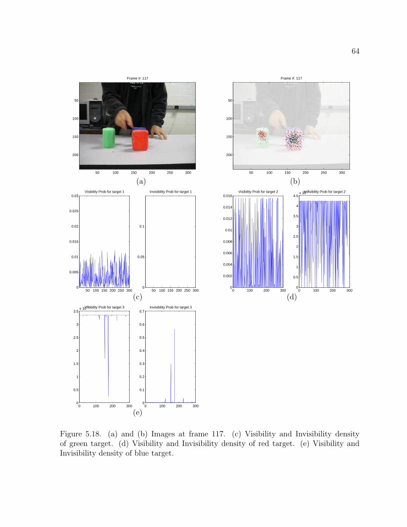
5.18 (a) and (b) Images at frame 117. (c), (d), and (e) are visibility and
invisibility density of green, red, and blue target, respectively . . . . . . 64
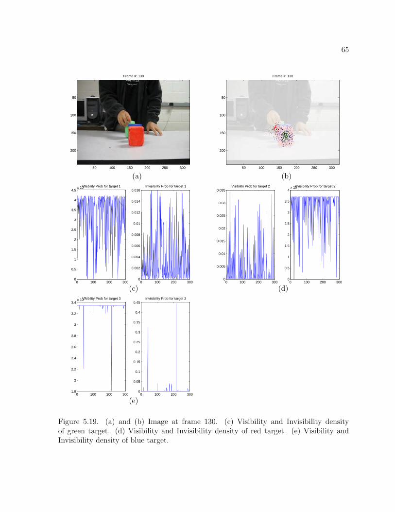
5.19 (a) and (b) Images at frame 130. (c), (d), and (e) are visibility andinvisibility density of green, red, and blue target, respectively . . . . . . . 65
5.20 (a) and (b) Images at frame 143. (c), (d), and (e) are visibility andinvisibility density of green, red, and blue target, respectively . . . . . . . 66
5.21 (a) and (b) Images at frame 184. (c), (d), and (e) are visibility andinvisibility density of green, red, and blue target, respectively . . . . . . . 67
5.22 Importance Weight Distribution for three targets . . . . . . . . . . . . . 69
5.25 (a) and (b) Mean of errors in Cartesian distance and error bars using thestandard Particle filter and multi-target Particle filter, respectively . . . . 73
5.26 Mean of errors in Cartesian distance and error bars using standard Particlefilter . . . . . . . . . . . . . . . . . . . . . . . . . . . . . . . . . . . . . . 74
In the probabilistic exclusion principle [18], a state was extended to contain two
objects: a foreground object and a background object. In a boosted particle filter [17],
the cascaded Adaboost algorithm was used to provide a mechanism for allowing ob-
jects leaving and entering the scene effectively. Similarly, [10] used the K-means spatial
reclustering algorithm for maintaining the targets by merging and splitting the clusters.
Since we do not use any clustering methods or do not extend the target states, which
may cause the complexity cost to grow exponentially, we need to provide an efficient
and effective method to obtain and maintain the target representation. To do this, we
propose a new method to evaluate the visibility likelihood in Equation 4.6. This method
consists of three steps: (1) project particles into the image space by accumulating each
particle weight over the corresponding pixels, (2) normalize each pixel with the summa-
tion of the accumulated weights from each target filter, (3) project back from the image
space to the particle space by re-normalizing the pixel weights over the target area of
the corresponding particles. What follows is a mathematical derivation of the three steps.
The visibility likelihood term is derived by using Bayes’ law as follows:
pk(Vk|xk,t, zt) =pk(zt|xk,t, Vk)pk(Vk|xk,t)
pk(zk|xk,t)(4.6)
The main idea of the first step in Equation 4.6 is to project the particle weights into the
image space. In other words, we translate this term to the following equation:
αpk(VkP ixWeight|Xk
P ixLoc, zt) =∑
xk,t|XPixLoc∈Pixel(xk,t)
pk(zt|xk,t, Vk) (4.7)
29
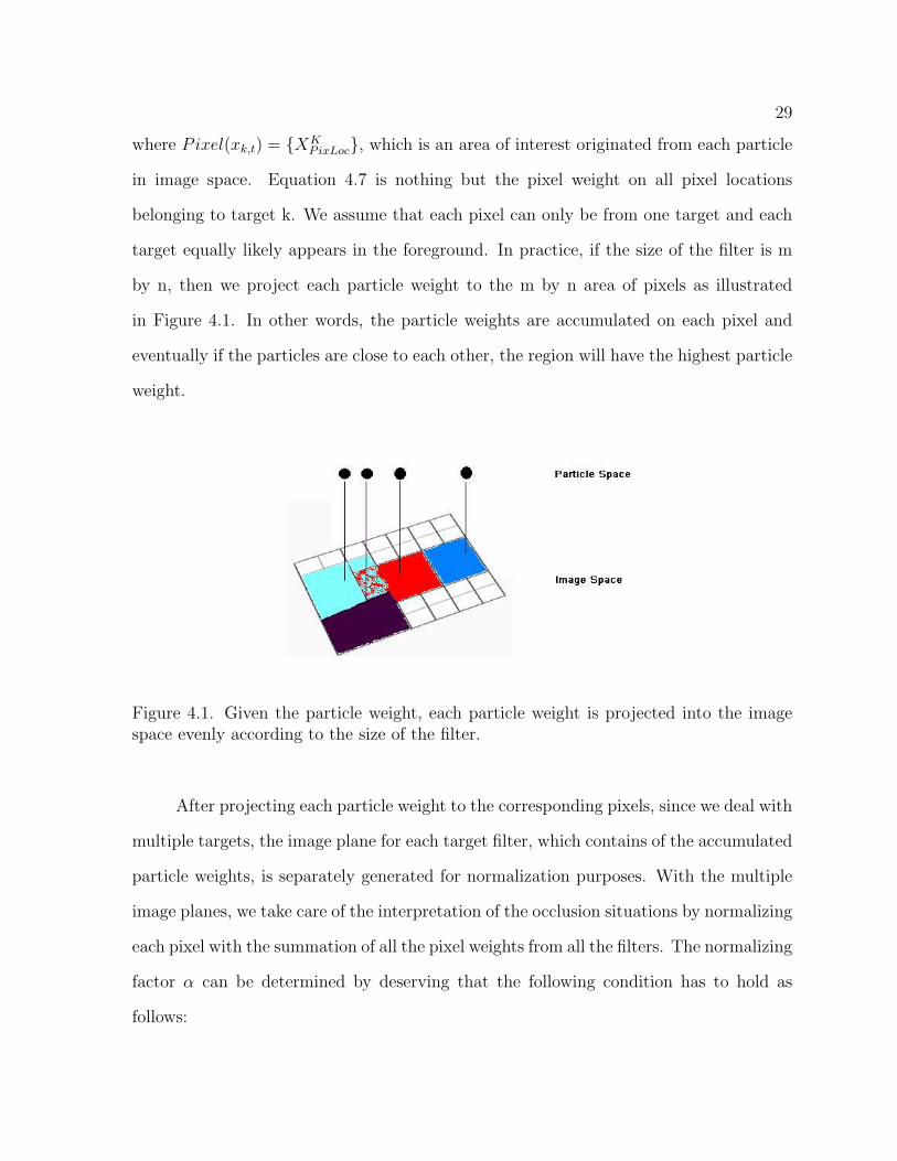
where Pixel(xk,t) = {XKPixLoc}, which is an area of interest originated from each particle
in image space. Equation 4.7 is nothing but the pixel weight on all pixel locations
belonging to target k. We assume that each pixel can only be from one target and each
target equally likely appears in the foreground. In practice, if the size of the filter is m
by n, then we project each particle weight to the m by n area of pixels as illustrated
in Figure 4.1. In other words, the particle weights are accumulated on each pixel and
eventually if the particles are close to each other, the region will have the highest particle
weight.
Figure 4.1. Given the particle weight, each particle weight is projected into the imagespace evenly according to the size of the filter.
After projecting each particle weight to the corresponding pixels, since we deal with
multiple targets, the image plane for each target filter, which contains of the accumulated
particle weights, is separately generated for normalization purposes. With the multiple
image planes, we take care of the interpretation of the occlusion situations by normalizing
each pixel with the summation of all the pixel weights from all the filters. The normalizing
factor α can be determined by deserving that the following condition has to hold as
follows:
30
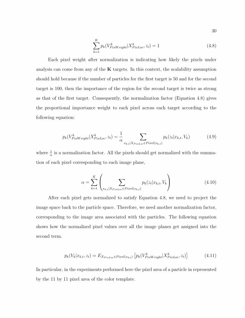
K∑
k=1
pk(VkP ixWeight|Xk
P ixLoc, zt) = 1 (4.8)
Each pixel weight after normalization is indicating how likely the pixels under
analysis can come from any of the K targets. In this context, the scalability assumption
should hold because if the number of particles for the first target is 50 and for the second
target is 100, then the importance of the region for the second target is twice as strong
as that of the first target. Consequently, the normalization factor (Equation 4.8) gives
the proportional importance weight to each pixel across each target according to the
following equation:
pk(VkP ixWeight|Xk
P ixLoc, zt) =1
α
∑
xk,t|XPixLoc∈Pixel(xk,t)
pk(zt|xk,t, Vk) (4.9)
where 1α
is a normalization factor. All the pixels should get normalized with the summa-
tion of each pixel corresponding to each image plane,
α =K∑
k=1
∑
xk,t|XPixLoc∈Pixel(xk,t)
pk(zt|xk,t, Vk
(4.10)
After each pixel gets normalized to satisfy Equation 4.8, we need to project the
image space back to the particle space. Therefore, we need another normalization factor,
corresponding to the image area associated with the particles. The following equation
shows how the normalized pixel values over all the image planes get assigned into the
second term.
pk(Vk|xk,t, zt) = EXPixLoc∈Pixel(xk,t)
[pk(V
kP ixWeight|Xk
P ixLoc, zt)]
(4.11)
In particular, in the experiments performed here the pixel area of a particle in represented
by the 11 by 11 pixel area of the color template.
31
4.2.2.2 Observation Model For Hidden Targets: pk(zt|xk,t, Vk)
The third term of Equation 4.4 requires a method for evaluating the measurement
support (likelihood) of occluded targets, whereas the first term is relatively easy to eval-
uate the measurement support of each target being visible. The important point of this
term is how to maintain the filtering distribution of each target without biasing the re-
sulting distribution and how to exploit the observation information even if the targets
are occluded by other targets or clutter. For this, we compute the third term not only
not to assign too much weight to occluded target,but also not to move too much weight
to the foreground target from the targets behind, by utilizing the expectation of the
measurement model pk(zk|xk,t, Vk) = Ezt [pk(zt|xk,t, Vk)].
4.2.3 Filter Deletion
This section presents the fundamental framework of filter deletion, which happens
when a target disappears out of the scene. Filter deletion does not automatically happen
in the cases where one target is located behind another target for a long time because
the invisibility likelihood explains an occlusion situation. But if the target being tracked
suddenly disappears out of the scene, then we initiate the filter deletion. As a result,
the filter used to track the targets should be destroyed for the sake of process efficiency.
Since the filters are not smart enough to know when to terminate themselves, we utilize
information to compute the proposed observation likelihood. In other words, we deter-
mine the likelihood , pk(Ftk|Zt), that the target associated with filter k exists and define
a threshold to decide when to destroy the target distribution upon the disappearance out
of the scene. The following equation is the concept of the likelihood that a target exists.
32
p(F tk|Zt) =
p(zt|F tk, Z
t−1)p(Fk|Zt−1)
p(zt|Zt−1)(4.12)
where the numerator indicates particle weights∑i
k πi and the denominator is the expected
value of observation model in the current filter E[p(zt|Ft)]. This value obtained from
Equation 4.12 together with a threshold is used to determine whether the tracked target
filter is destroyed or not.
4.2.4 Filter Creation
Creation of another target filter is achieved through the addition of an additional
filter, called background filter. The background filer has to track what other filters do not
track. In order for this background filter not to represent the target of the other filters,
we use the visibility likelihood model described in section 4.2.2.1, but do not apply the
normalization procedures so that the background filter never bias on visibility likelihood
of other targets.
Each particle in the background filer randomly gets assigned one of the measure-
ment models being tracked. In order to prevent the background filter from tracking
targets already traced by other filters have to be considered, operation happens in the
image plane by removing all the pixels in the image plane of the background filter which
cover regions that are already being tracked by other filters. This means that we never
find objects that are partially overlapped by others. Then, how do we find a cluster that
might be a potential target that other filters are not tracking? The simplest solution
for detecting the cluster that other filters are not tracking is to use a density estimate
by computing the highest pixel weight of the background filter in the image space and
33
compare it to a stationary threshold. If the weight of the cluster in the image plane of the
background filter does exceed the significance threshold, we create a filter for that target.
The important element to note here after finding new target is that we have to transform
the current state of the background filter to the new filter including the observation model.
To make target finding more efficient and to avoid the depletion problem, once the
background filter falls into one of the targets that has already been tracked by other filters,
we bias the distribution of the background filter by resampling a half or 60 percentage
of the particles in the resampling step and replacing the rest with random new particles
so that it easily starts to search a new target.
4.3 Computational Complexity
With the assumption that a target is a rigid object and not transparent, the key to
a robust multi-target occlusion observation model in the proposed method is to project
the particle weight to each corresponding pixel and introduce a normalization factor to
include occlusion situations. As particles in the joint particle filter contain the joint
position of all targets and the filter thus suffers from exponential complexity with the
increasing number of targets, we proposed a pixel-based computation technique not only
to help the proposed observation likelihood model (Equation 4.2) to explain the possible
occlusions, but also to reduce the complexity of the filter to linear in the number of
targets.
The important point to note in the proposed method is that the computational com-
plexity does not increase exponentially even though the number of targets is increased.
In this thesis, the only element that is required to be computed is the interaction of
the importance weights. This means that we only need to worry about the observation
34
model, which is the first and second term in Equation 4.5. How do we compute these
terms without increasing the computational complexity? In what follows, we first discuss
why the joint particle filter is intractable and inefficient when it handles the occlusion
situations and discuss how the proposed method with its observation model provides a
computation cost that grows linearly while approximating a joint distribution. by utiliz-
ing the pixel-based computation.
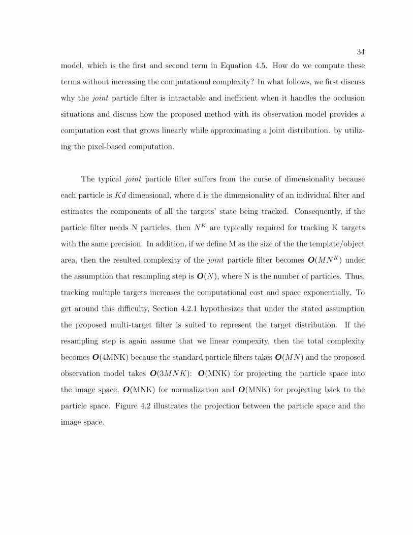
The typical joint particle filter suffers from the curse of dimensionality because
each particle is Kd dimensional, where d is the dimensionality of an individual filter and
estimates the components of all the targets’ state being tracked. Consequently, if the
particle filter needs N particles, then NK are typically required for tracking K targets
with the same precision. In addition, if we define M as the size of the the template/object
area, then the resulted complexity of the joint particle filter becomes O(MNK) under
the assumption that resampling step is O(N), where N is the number of particles. Thus,
tracking multiple targets increases the computational cost and space exponentially. To
get around this difficulty, Section 4.2.1 hypothesizes that under the stated assumption
the proposed multi-target filter is suited to represent the target distribution. If the
resampling step is again assume that we linear compexity, then the total complexity
becomes O(4MNK) because the standard particle filters takes O(MN) and the proposed
observation model takes O(3MNK): O(MNK) for projecting the particle space into
the image space, O(MNK) for normalization and O(MNK) for projecting back to the
particle space. Figure 4.2 illustrates the projection between the particle space and the
image space.
35
Figure 4.2. Projection step between the particle space and the image space. (1) Projec-tion into image plane. (2) Normalization of each pixel. (3) Re-normalization of all thenormalized pixels..
4.4 SIR Multi-Target Particle Filter
This section describes the detailed steps of the distributed multi-target Particle
filter algorithm.
• INITIALIZATION
At time t-1, the state of the targets is represented by a set of unweighted samples
{xik,t−1}N
i=1, where N is the number of the samples. Each target has a set of these
samples.
• FOR EACH TARGET k : K
1. Evaluate the observation likelihood {xik,t}N
i=1.
36
2. Construct the Image Plane for each target k by normalizing each pixel in each
image plane according to Equation 4.9 and Equation 4.11.
3. Calculate the expected value of the measurement model.
4. Calculate the fourth term in Equation 4.5 : 1 - pk(Vk|xk,t, F∀K).
5. Compute the importance weight distribution {πik}N
i=1 by assigning the values
from the above four steps into Equation 4.5.
• END
• RESAMPLING STEP
– FOR EACH TARGET k : K
∗ Resample each target state {xik,t}N
i=1 according to Table (2.2).
– END
• END
• The resulting sample sets {xik,t, π
ik,t} for each target at time t represents an esti-
mated state of the targets.
CHAPTER 5
EXPERIMENTAL RESULTS
This chapter describes the state-space models, the observation models, and expec-
tation of the observation model. For experiments, we compare the performance of the
proposed multi-target particle filter with that of the standard particle filter on three dif-
ferent tracking problems. The first experiment demonstrates the standard Particle filter
over multiple targets. The second are three tracking examples with different numbers of
targets using the proposed multi-target Particle filter. The last shows examples of filter
deletion and creation. All the experiments are performed on a video sequence.
5.1 State Space Model
There is significant literature related to multi-target tracking. Even though all the
literature has different ways to address the tracking problem, the way of approximat-
ing the state space generally falls into one of two categories. The first uses the general
way such that the states consist of the image coordinates (i.e. xy plane), velocity, or
acceleration of targets, e.g. [2,3]. In the context of multi-target tracking we assume
that the number of targets to be tracked, K, varies and is known a priori. Each target
is parameterized by the state xk,t, {k = 1...K}, which has different configurations (i.e.
different image coordinates) for the individual targets. The representation of multiple
targets Xk is given by the individual target states, i.e. Xk = (x1,t, . . . , xK,t). In the
experiment, the targets are rectangular boxes. We therefore define the particle represen-
tation of each state as xk,t = {xt, yt} where x, y specify the location of the samples. The
37
38
particle representation has two degrees of freedom, one in each direction of the image
coordinates.
5.2 Observation Likelihood Model
This section describes the likelihood model pk(zt|Xk,t) where zt is a likelihood eval-
uated by the observation model (color-based observation model in the experiment) and
Xk,t is the position of objects. In short, the observation likelihood model pk(zt|Xk,t)
expresses the likelihood of target k given that the objects would be located at Xk,t. The
observation likelihood values (i.e. probabilistic measurement of similarity between zk,t
and reference features) do not only arise from the targets to be tracked, but also addi-
tional clutter likelihood may result due to spurious objects, background changes, etc. We
will assume that each of the targets can generate at most one likelihood at a particular
time step. The likelihood model we will use for our experiments is a color likelihood
model that was proposed in [15, 24] and the following section explains it in detail.
5.2.1 Color Likelihood Model
The color likelihood model [15] generates a measurement of similarity by compar-
ing the color histogram of candidate regions in the current scene to a reference color
histogram. We build color models by utilizing the color histogram method in the Hue-
Saturation-Value (HSV) color space in order to decouple chromatic information from
shading effects. We measure the likelihood through the Bhattacharyya distance between
the two HSV color histograms of the reference and the candidate models.
Suppose that the distributions of the color histogram are transformed into m bins.
The function h(xi) produces the histograms that associate the color at location xi to the
corresponding bin. In our experiments, we transform the histogram in RGB color space
39
to a HSV color histogram using 8 × 8 × 4 bins to make the histogram less sensitive to
lighting conditions.
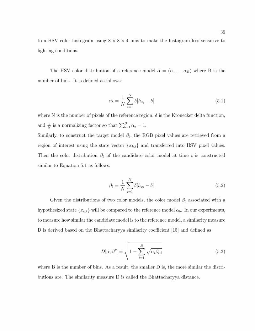
The HSV color distribution of a reference model α = (α1, ..., αB) where B is the
number of bins. It is defined as follows:
αb =1
N
N∑i=1
δ[hxi− b] (5.1)
where N is the number of pixels of the reference region, δ is the Kronecker delta function,
and 1N
is a normalizing factor so that∑B
b=1 αb = 1.
Similarly, to construct the target model βb, the RGB pixel values are retrieved from a
region of interest using the state vector {xk,t} and transferred into HSV pixel values.
Then the color distribution βb of the candidate color model at time t is constructed
similar to Equation 5.1 as follows:
βb =1
N
N∑i=1
δ[hxi− b] (5.2)
Given the distributions of two color models, the color model βb associated with a
hypothesized state {xk,t} will be compared to the reference model αb. In our experiments,
to measure how similar the candidate model is to the reference model, a similarity measure
D is derived based on the Bhattacharyya similarity coefficient [15] and defined as
D[α, βt] =
√√√√1−B∑
i=1
√αiβt,i (5.3)
where B is the number of bins. As a result, the smaller D is, the more similar the distri-
butions are. The similarity measure D is called the Bhattacharyya distance.
40
Since the smaller distance corresponds to the larger weight, we use the normal
distribution to evaluate the likelihood between the two distributions. In the context of
the particle filter, the weight πik in the samples (xi
k, πik) is evaluated using the following
normal distribution:
πik(D) =
1√2πσ
e−D2
2σ2 (5.4)
where the width of the likelihood is controlled by the variance parameter σ2 in the
function of D. In our experiments, this standard deviation is assigned 17. A similar model
was already implemented in the context of the object tracking in [15, 21, 25]. Note that
as the Bhattacharyya distance D can only take values between 0 and 1, πik(D) does not
strictly represent a probability density, but would have to be scaled using 1R 10 πi
k(D). Due
to the normalization in the filter, however, constant is not required during calculation.
5.2.2 Compute Expected Observation Model
Chapter 4 explains the filtering distribution in a form of a probability density
function (pdf) p(xk,t|Zt) where k = {1 ... K} is the number of the targets. In partic-
ular, Equation 4.5 requires computation of the four related terms. This section shows
a mathematical solution of the third term (pk(zt|xk,t, Vk)), which is an expectation of
the observation model Ezt [pk(zt|xk,t, Vk)] described in Chapter 4. We mathematically
evaluate the expected value of the observation model as follow:
41
pk(zt|xk,t, Vk) = ED
[πi
k(D)]
=
∫ 1
0
πik(D)p(D)dD
=
∫ 1
0
[1√2πσ
e−D2
2σ2
]2
dD
=1
2πσ2− σ2
[e−
(D2)
σ2
]1
0
=−1
2π
(e−1σ2 − 1
)
(5.5)
where σ is given 17, the range of a function of D is [0,1], and p(x) is considered as the
same distribution of πik(D) in this case. However, the expected value obtained from
Equation 5.5 might not be a right value because our assumption is that Equation 5.4 is
the distribution in a real image and therefore integrates to one because it is a probability
function. This, however, is not the case here because we are using only a part of the
Gaussian distribution. Eventually, we scale p(D), the second term of the second line
in Equation 5.5, to be a density function. However, since p(D) does not measure the
exact distribution in a real image, we alternatively determined this value by experiments.
Eventually, this value is defined as 0.0000036 in the standard Particle filter and used for
the expected value of the observation model. For the practical experiments, we use
slightly lower value than 0.0000036 to bias the filter toward targets and then to reduce
the time required for the particles to collapse into each target.
5.3 Experimental Results
As a benchmark, we compare the proposed multi-target Particle filters against
standard Particle filters using the same objects. In the standard Particle filters, the
experiments are performed by tracking multiple targets and the results are the precision in
42
terms of tracking accuracy. To compute the precision of tracking the targets, we manually
track the center positions of each target and compare them against the expected value
of the locations of the samples. The density estimate is used to calculate the position of
the targets. Since it is well known that the precision of tracking gets much better with
the increase in the number of the particles [22, 8], we do not include experimental results
with different number of the particles. Instead, we focus on the precision and capability
to track multiple targets as the number of targets increases. Targets are rectangular
boxes in different colors (i.e., red, green, and blue) on image sequences recorded at a
constant frame rate of 15 frames per second and with images of size 320 by 240 in RGB
color space. The template used for the observation model consists of 11 by 11 pixels. The
experiments for the proposed algorithm are performed with different numbers of targets.
We mainly evaluate the precision in terms of the number of targets and the tractability
of the occlusion situations. Finally, we show experimental results for a filter deletion and
creation. Note that some experiments with high particle numbers did not run in real
time.
5.3.1 Standard Particle Filters
In this experiment, the standard Particle filter runs to track the rectangular boxes
of the same color. The targets move around in the cluttered background and sometimes
disappear and appear again as shown in Figure 5.1. Below is the specific implementation
information.
• The state xk,t of the kth target consists of its position (xk,t, yk,t) in the image.
• For the observation likelihood model, we used an appearance template approach.
In particular, we used a 11 by 11 square template containing the reference image
transformed into HSV color space.
43
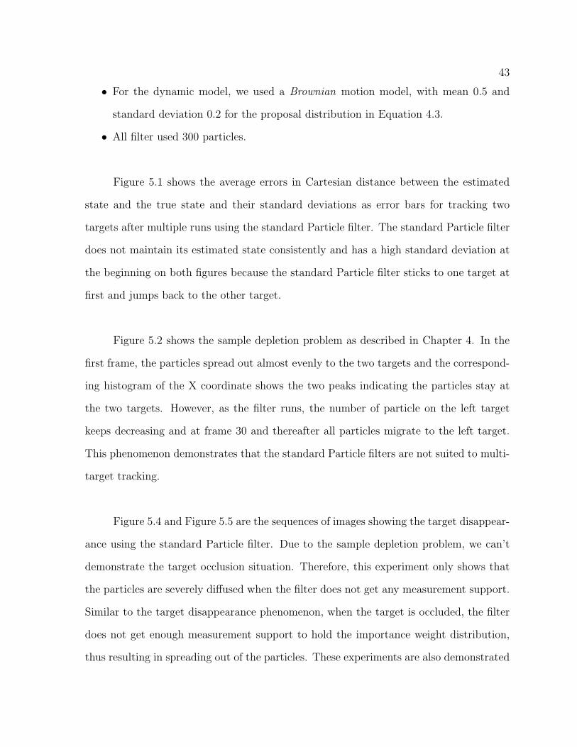
• For the dynamic model, we used a Brownian motion model, with mean 0.5 and
standard deviation 0.2 for the proposal distribution in Equation 4.3.
• All filter used 300 particles.
Figure 5.1 shows the average errors in Cartesian distance between the estimated
state and the true state and their standard deviations as error bars for tracking two
targets after multiple runs using the standard Particle filter. The standard Particle filter
does not maintain its estimated state consistently and has a high standard deviation at
the beginning on both figures because the standard Particle filter sticks to one target at
first and jumps back to the other target.
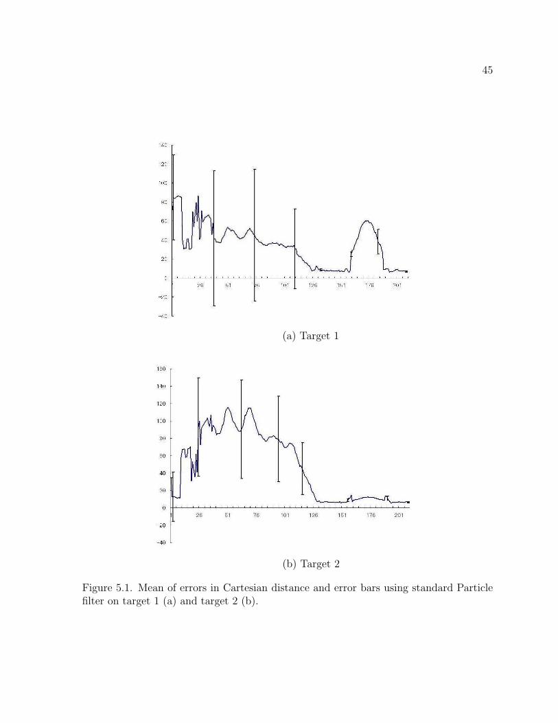
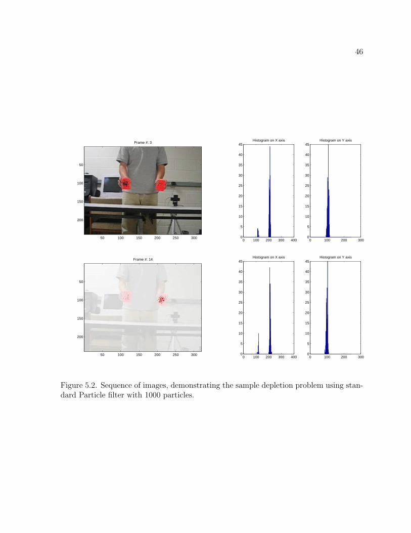
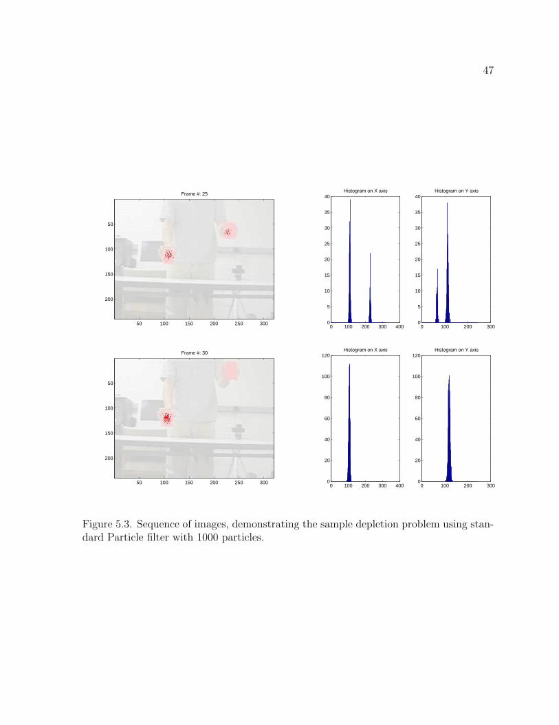
Figure 5.2 shows the sample depletion problem as described in Chapter 4. In the
first frame, the particles spread out almost evenly to the two targets and the correspond-
ing histogram of the X coordinate shows the two peaks indicating the particles stay at
the two targets. However, as the filter runs, the number of particle on the left target
keeps decreasing and at frame 30 and thereafter all particles migrate to the left target.
This phenomenon demonstrates that the standard Particle filters are not suited to multi-
target tracking.
Figure 5.4 and Figure 5.5 are the sequences of images showing the target disappear-
ance using the standard Particle filter. Due to the sample depletion problem, we can’t
demonstrate the target occlusion situation. Therefore, this experiment only shows that
the particles are severely diffused when the filter does not get any measurement support.
Similar to the target disappearance phenomenon, when the target is occluded, the filter
does not get enough measurement support to hold the importance weight distribution,
thus resulting in spreading out of the particles. These experiments are also demonstrated
44
in the next subsection over distributed multi-target Particle filters. At frame 37 of Figure
5.2, when the target is about to disappear, the particles start to spread. At frame 51 of
Figure 5.3, the diffusion of the particles is very severe and finally they are back on the
target when the target appears again at frame 65.
45
(a) Target 1
(b) Target 2
Figure 5.1. Mean of errors in Cartesian distance and error bars using standard Particlefilter on target 1 (a) and target 2 (b).
46
Frame #: 3
50 100 150 200 250 300
50
100
150
200
0 100 200 300 4000
5
10
15
20
25
30
35
40
45Histogram on X axis
0 100 200 3000
5
10
15
20
25
30
35
40
45Histogram on Y axis
Frame #: 14
50 100 150 200 250 300
50
100
150
200
0 100 200 300 4000
5
10
15
20
25
30
35
40
45Histogram on X axis
0 100 200 3000
5
10
15
20
25
30
35
40
45Histogram on Y axis
Figure 5.2. Sequence of images, demonstrating the sample depletion problem using stan-dard Particle filter with 1000 particles.
47
Frame #: 25
50 100 150 200 250 300
50
100
150
200
0 100 200 300 4000
5
10
15
20
25
30
35
40Histogram on X axis
0 100 200 3000
5
10
15
20
25
30
35
40Histogram on Y axis
Frame #: 30
50 100 150 200 250 300
50
100
150
200
0 100 200 300 4000
20
40
60
80
100
120Histogram on X axis
0 100 200 3000
20
40
60
80
100
120Histogram on Y axis
Figure 5.3. Sequence of images, demonstrating the sample depletion problem using stan-dard Particle filter with 1000 particles.
48
Frame #: 3
50 100 150 200 250 300
50
100
150
200
0 100 200 300 4000
20
40
60
80
100
120Histogram on X axis
0 100 200 3000
10
20
30
40
50
60
70
80
90
100Histogram on Y axis
Frame #: 30
50 100 150 200 250 300
50
100
150
200
0 100 200 300 4000
20
40
60
80
100
120Histogram on X axis
0 100 200 3000
20
40
60
80
100
120
140Histogram on Y axis
Frame #: 35
50 100 150 200 250 300
50
100
150
200
0 100 200 300 4000
10
20
30
40
50
60Histogram on X axis
0 100 200 3000
20
40
60
80
100
120
140
160
180Histogram on Y axis
Figure 5.4. Target disappearance experiment using standard Particle filter with 1000particles.
49
Frame #: 37
50 100 150 200 250 300
50
100
150
200
0 100 200 300 4000
5
10
15
20
25
30
35
40
45Histogram on X axis
0 100 200 3000
20
40
60
80
100
120Histogram on Y axis
Frame #: 39
50 100 150 200 250 300
50
100
150
200
0 100 200 300 4000
5
10
15
20
25
30Histogram on X axis
0 100 200 3000
20
40
60
80
100
120Histogram on Y axis
Frame #: 51
50 100 150 200 250 300
50
100
150
200
0 100 200 300 4000
5
10
15
20
25Histogram on X axis
0 100 200 3000
10
20
30
40
50
60
70
80
90Histogram on Y axis
Figure 5.5. Target disappearance experiment using standard Particle filter with 1000particles.
50
Frame #: 63
50 100 150 200 250 300
50
100
150
200
0 100 200 300 4000
20
40
60
80
100
120Histogram on X axis
0 100 200 3000
10
20
30
40
50
60
70
80Histogram on Y axis
Frame #: 65
50 100 150 200 250 300
50
100
150
200
0 100 200 300 4000
10
20
30
40
50
60
70
80
90
100Histogram on X axis
0 100 200 3000
20
40
60
80
100
120Histogram on Y axis
Figure 5.6. Target disappearance experiment using standard Particle filter with 1000particles.
51
5.3.2 Distributed Multi-Target Particle Filter
The proposed algorithm is implemented according to the pseudo code algorithm in
Section 4.4. The experimental setup is the same as that the standard Particle filter. This
subsection consists of three different experiments: tracking two targets, tracking three
targets, and target deletion and creation. Figures mainly illustrate the precision of the
target trajectories against the true target trajectories and occlusion situations. The true
state is manually estimated.
5.3.2.1 Tracking Two Targets of Different Color
Figure 5.7 shows the same information as Figure 5.1 but using the proposed multi-
target Particle filter. The proposed distributed multi-target Particle filter is capable of
tracking all the targets by maintaining low standard deviation between a true state and
an estimated state. Therefore, it is well suited to tracking multiple targets.
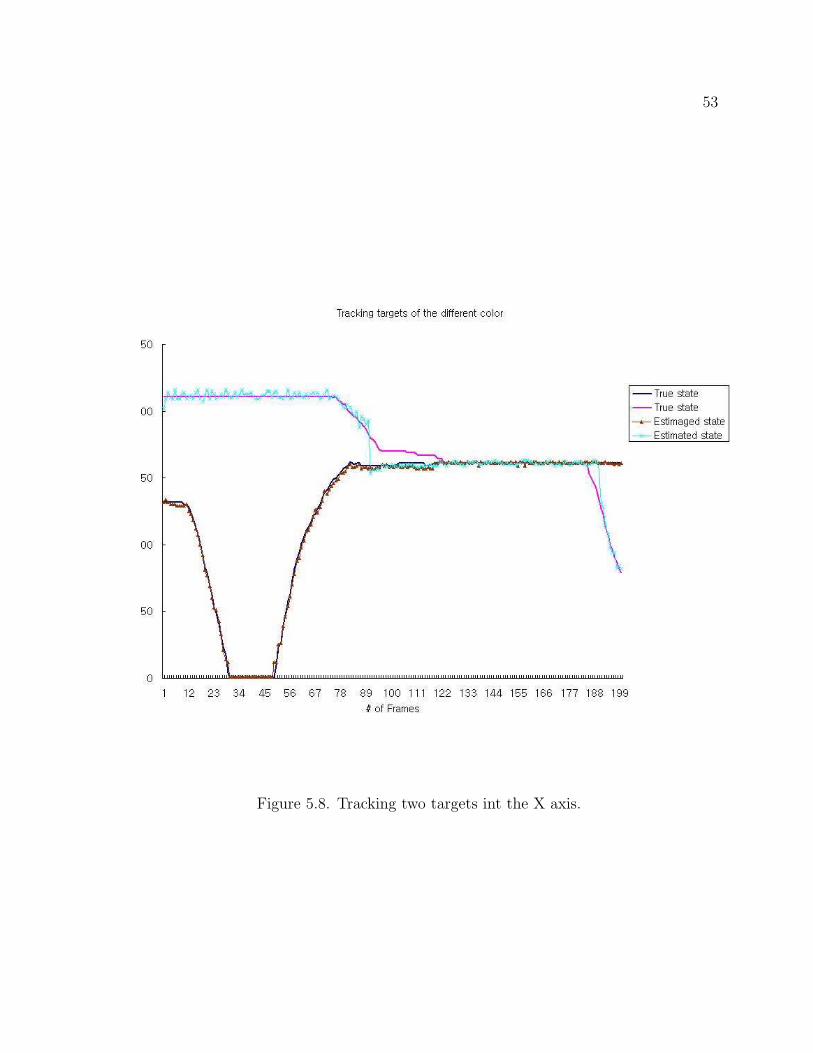
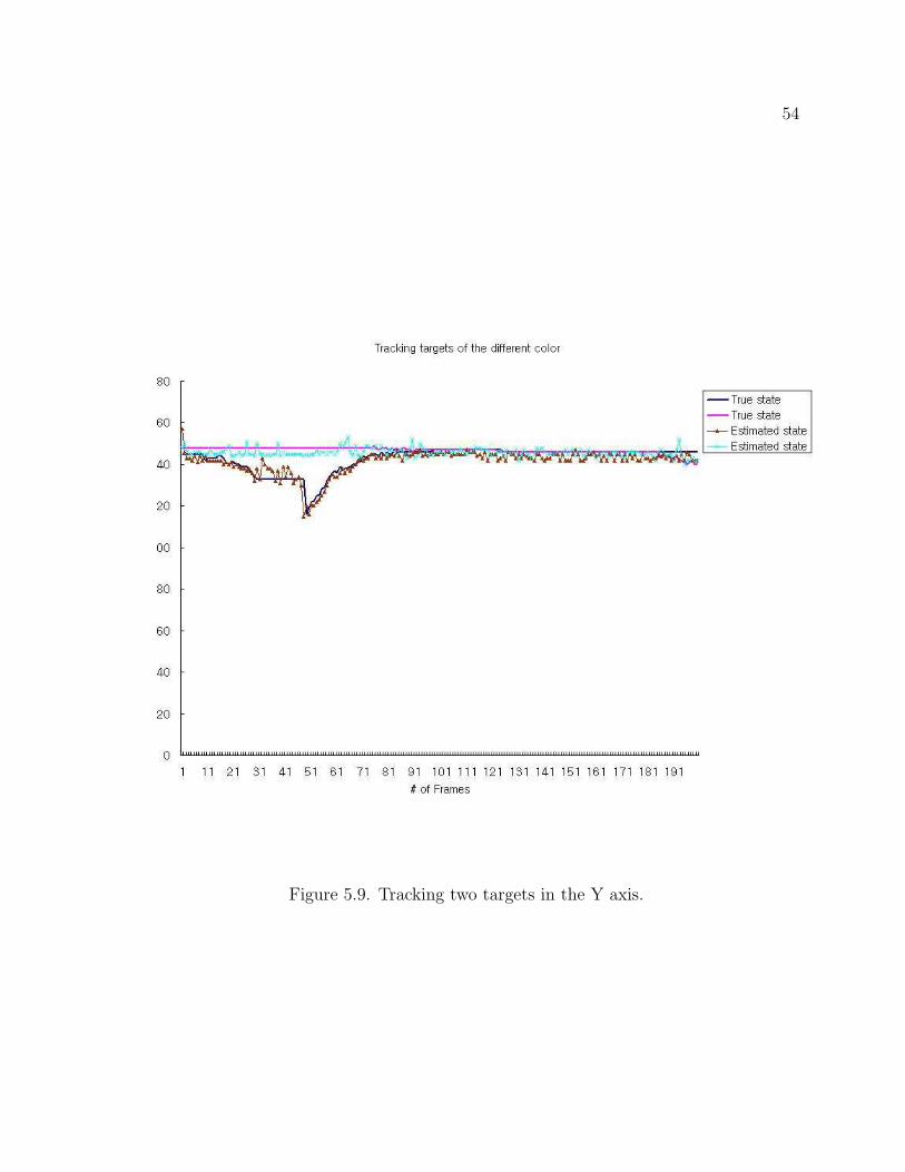
Figure 5.8 and Figure 5.9 describe trajectories of a red and green target in the X
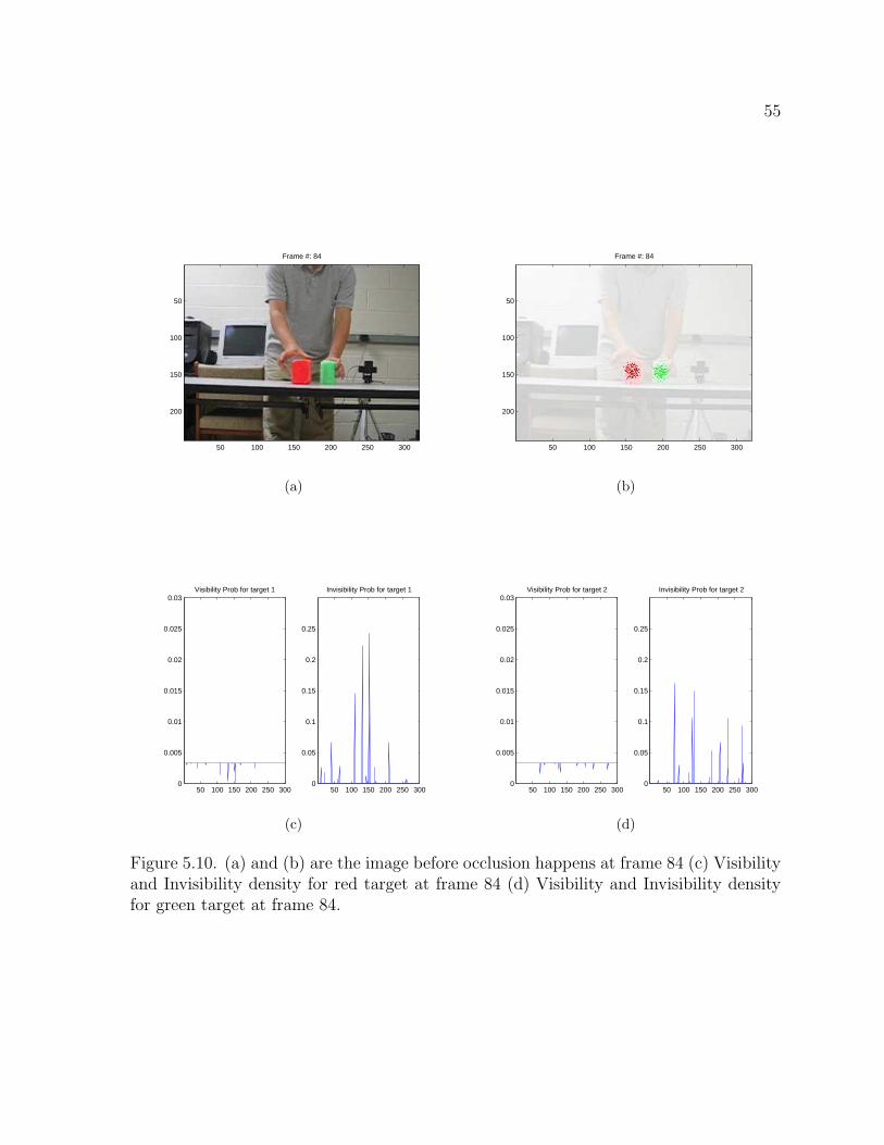
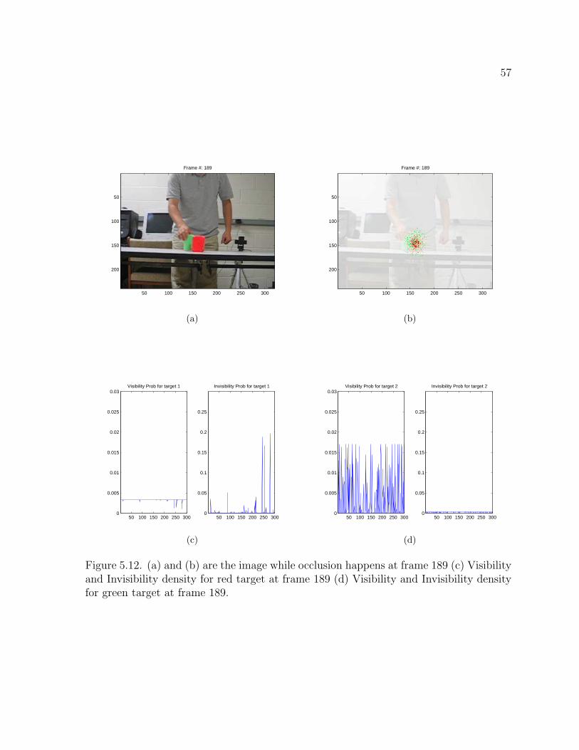
and Y axis. Figure 5.10 to Figure 5.13 show a sequence of tracking images and their
corresponding visibility and invisibility density for each target. While the green target
passes behind the red target, the invisibility probability density explains the occlusion
situation by increasing the density when the occlusion happens, and otherwise decreasing
the density in case of no occlusion. Figure 5.10 (b) indicates that Invisibility density starts
to increase and after the green target is not occluded its density dramatically drops to
almost zero.
52
(a) Target 1
(b) Target 2
Figure 5.7. Mean errors in Cartesian distance and error bars using multi-target Particlefilter on target 1 (a) and target 2 (b).
53
Figure 5.8. Tracking two targets int the X axis.
54
Figure 5.9. Tracking two targets in the Y axis.
55
Frame #: 84
50 100 150 200 250 300
50
100
150
200
(a)
Frame #: 84
50 100 150 200 250 300
50
100
150
200
(b)
50 100 150 200 250 3000
0.005
0.01
0.015
0.02
0.025
0.03Visibility Prob for target 1
50 100 150 200 250 3000
0.05
0.1
0.15
0.2
0.25
Invisibility Prob for target 1
(c)
50 100 150 200 250 3000
0.005
0.01
0.015
0.02
0.025
0.03Visibility Prob for target 2
50 100 150 200 250 3000
0.05
0.1
0.15
0.2
0.25
Invisibility Prob for target 2
(d)
Figure 5.10. (a) and (b) are the image before occlusion happens at frame 84 (c) Visibilityand Invisibility density for red target at frame 84 (d) Visibility and Invisibility densityfor green target at frame 84.
56
Frame #: 91
50 100 150 200 250 300
50
100
150
200
(a)
Frame #: 91
50 100 150 200 250 300
50
100
150
200
(b)
50 100 150 200 250 3000
0.005
0.01
0.015
0.02
0.025
0.03Visibility Prob for target 1
50 100 150 200 250 3000
0.05
0.1
0.15
0.2
0.25
Invisibility Prob for target 1
(c)
50 100 150 200 250 3000
0.005
0.01
0.015
0.02
0.025
0.03Visibility Prob for target 2
50 100 150 200 250 3000
0.05
0.1
0.15
0.2
0.25
Invisibility Prob for target 2
(d)
Figure 5.11. (a) and (b) are the image while occlusion happens at frame 91 (c) Visibilityand Invisibility density for red target at frame 91 (d) Visibility and Invisibility densityfor green target at frame 91.
57
Frame #: 189
50 100 150 200 250 300
50
100
150
200
(a)
Frame #: 189
50 100 150 200 250 300
50
100
150
200
(b)
50 100 150 200 250 3000
0.005
0.01
0.015
0.02
0.025
0.03Visibility Prob for target 1
50 100 150 200 250 3000
0.05
0.1
0.15
0.2
0.25
Invisibility Prob for target 1
(c)
50 100 150 200 250 3000
0.005
0.01
0.015
0.02
0.025
0.03Visibility Prob for target 2
50 100 150 200 250 3000
0.05
0.1
0.15
0.2
0.25
Invisibility Prob for target 2
(d)
Figure 5.12. (a) and (b) are the image while occlusion happens at frame 189 (c) Visibilityand Invisibility density for red target at frame 189 (d) Visibility and Invisibility densityfor green target at frame 189.
58
Frame #: 201
50 100 150 200 250 300
50
100
150
200
(a)
Frame #: 201
50 100 150 200 250 300
50
100
150
200
(b)
50 100 150 200 250 3000
0.005
0.01
0.015
0.02
0.025
0.03Visibility Prob for target 1
50 100 150 200 250 3000
0.05
0.1
0.15
0.2
0.25
Invisibility Prob for target 1
(c)
50 100 150 200 250 3000
0.005
0.01
0.015
0.02
0.025
0.03Visibility Prob for target 2
50 100 150 200 250 3000
0.05
0.1
0.15
0.2
0.25
Invisibility Prob for target 2
(d)
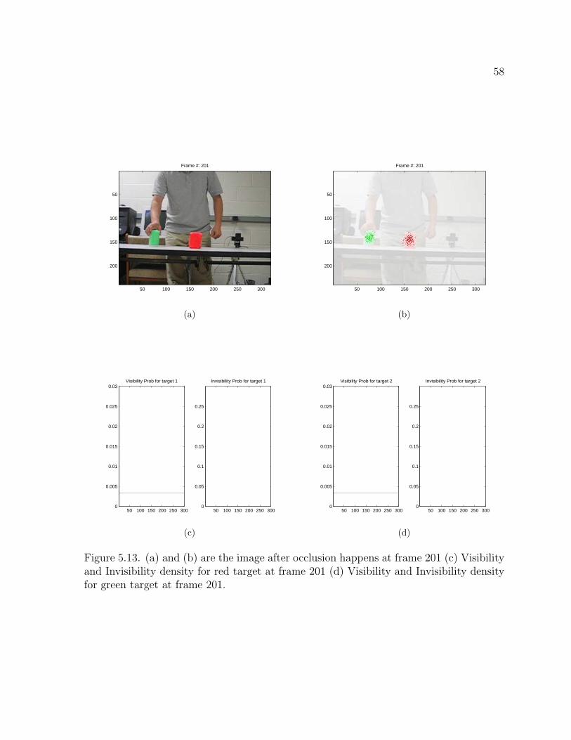
Figure 5.13. (a) and (b) are the image after occlusion happens at frame 201 (c) Visibilityand Invisibility density for red target at frame 201 (d) Visibility and Invisibility densityfor green target at frame 201.
59
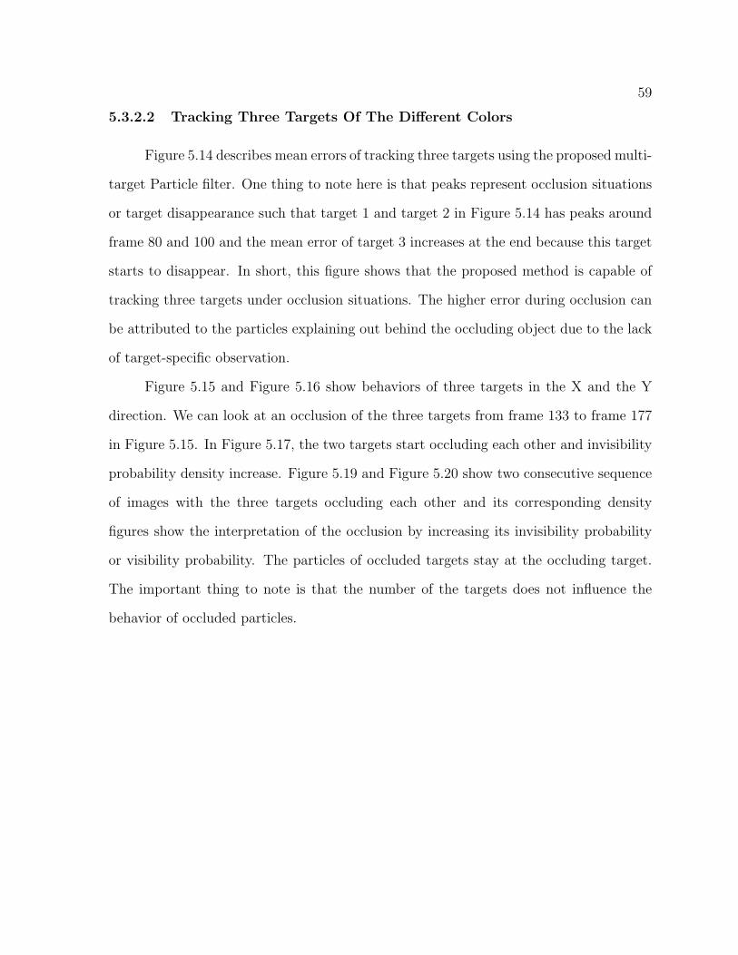
5.3.2.2 Tracking Three Targets Of The Different Colors
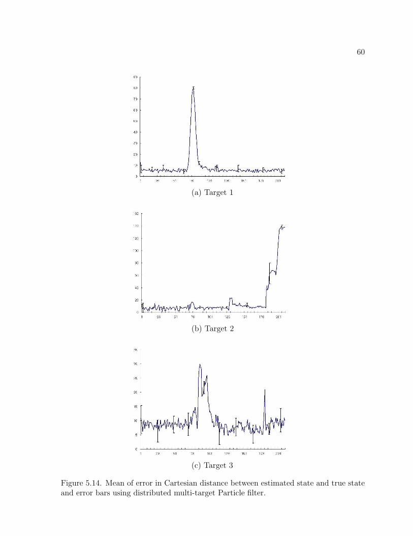
Figure 5.14 describes mean errors of tracking three targets using the proposed multi-
target Particle filter. One thing to note here is that peaks represent occlusion situations
or target disappearance such that target 1 and target 2 in Figure 5.14 has peaks around
frame 80 and 100 and the mean error of target 3 increases at the end because this target
starts to disappear. In short, this figure shows that the proposed method is capable of
tracking three targets under occlusion situations. The higher error during occlusion can
be attributed to the particles explaining out behind the occluding object due to the lack
of target-specific observation.
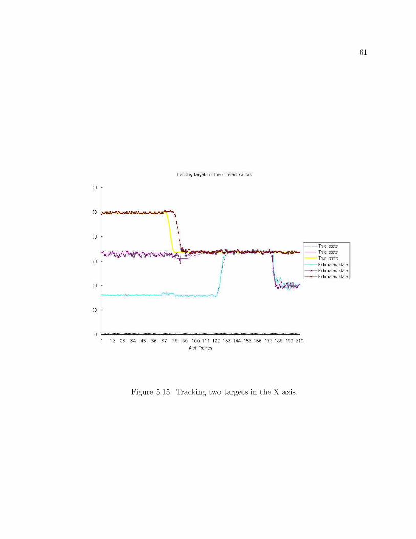
Figure 5.15 and Figure 5.16 show behaviors of three targets in the X and the Y
direction. We can look at an occlusion of the three targets from frame 133 to frame 177
in Figure 5.15. In Figure 5.17, the two targets start occluding each other and invisibility
probability density increase. Figure 5.19 and Figure 5.20 show two consecutive sequence
of images with the three targets occluding each other and its corresponding density
figures show the interpretation of the occlusion by increasing its invisibility probability
or visibility probability. The particles of occluded targets stay at the occluding target.
The important thing to note is that the number of the targets does not influence the
behavior of occluded particles.
60
(a) Target 1
(b) Target 2
(c) Target 3
Figure 5.14. Mean of error in Cartesian distance between estimated state and true stateand error bars using distributed multi-target Particle filter.
61
Figure 5.15. Tracking two targets in the X axis.
62
Figure 5.16. Tracking two targets in the Y axis.
63
(a)
Frame #: 83
50 100 150 200 250 300
50
100
150
200
(b)
Frame #: 83
50 100 150 200 250 300
50
100
150
200
(c)0 100 200 300
−1
−0.5
0
0.5
1
1.5Visibility Prob for target 1
0 100 200 3000
0.1
0.2
0.3
0.4
0.5
0.6
0.7
0.8
0.9
1Invisibility Prob for target 1
(d)0 100 200 300
1.8
2
2.2
2.4
2.6
2.8
3
3.2
3.4x 10
−3Visibility Prob for target 2
0 100 200 3000
0.05
0.1
0.15
0.2
0.25Invisibility Prob for target 2
(e)0 100 200 300
3.3332
3.3332
3.3333
3.3333
3.3333
3.3333
3.3333
3.3333
3.3333
3.3333
3.3333x 10
−3Visibility Prob for target 3
0 100 200 3000
0.1
0.2
0.3
0.4
0.5
0.6
0.7Invisibility Prob for target 3
Figure 5.17. (a) and (b) Images at frame 83. (c) Visibility and Invisibility density of greentarget. (d) Visibility and Invisibility density of red target. (e) Visibility and Invisibilitydensity of blue target.
64
(a)
Frame #: 117
50 100 150 200 250 300
50
100
150
200
(b)
Frame #: 117
50 100 150 200 250 300
50
100
150
200
(c)50 100 150 200 250 300
0
0.005
0.01
0.015
0.02
0.025
0.03Visibility Prob for target 1
50 100 150 200 250 3000
0.05
0.1
Invisibility Prob for target 1
(d)0 100 200 300
0
0.002
0.004
0.006
0.008
0.01
0.012
0.014
0.016Visibility Prob for target 2
0 100 200 3000
0.5
1
1.5
2
2.5
3
3.5
4
4.5x 10
−3Invisibility Prob for target 2
(e)0 100 200 300
0
0.5
1
1.5
2
2.5
3
3.5x 10
−3Visibility Prob for target 3
0 100 200 3000
0.1
0.2
0.3
0.4
0.5
0.6
0.7Invisibility Prob for target 3
Figure 5.18. (a) and (b) Images at frame 117. (c) Visibility and Invisibility densityof green target. (d) Visibility and Invisibility density of red target. (e) Visibility andInvisibility density of blue target.
65
(a)
Frame #: 130
50 100 150 200 250 300
50
100
150
200
(b)
Frame #: 130
50 100 150 200 250 300
50
100
150
200
(c)0 100 200 300
0
0.5
1
1.5
2
2.5
3
3.5
4
4.5x 10
−3Visibility Prob for target 1
0 100 200 3000
0.002
0.004
0.006
0.008
0.01
0.012
0.014
0.016Invisibility Prob for target 1
(d)0 100 200 300
0
0.005
0.01
0.015
0.02
0.025
0.03
0.035Visibility Prob for target 2
0 100 200 3000
0.5
1
1.5
2
2.5
3
3.5
4x 10
−3Invisibility Prob for target 2
(e)0 100 200 300
1.8
2
2.2
2.4
2.6
2.8
3
3.2
3.4x 10
−3Visibility Prob for target 3
0 100 200 3000
0.05
0.1
0.15
0.2
0.25
0.3
0.35
0.4
0.45Invisibility Prob for target 3
Figure 5.19. (a) and (b) Image at frame 130. (c) Visibility and Invisibility densityof green target. (d) Visibility and Invisibility density of red target. (e) Visibility andInvisibility density of blue target.
66
(a)
Frame #: 143
50 100 150 200 250 300
50
100
150
200
(a)
Frame #: 143
50 100 150 200 250 300
50
100
150
200
(b)0 100 200 300
0
0.005
0.01
0.015
0.02
0.025Visibility Prob for target 1
0 100 200 3000
0.5
1
1.5
2
2.5
3
3.5
4x 10
−3Invisibility Prob for target 1
(c)0 100 200 300
0
0.005
0.01
0.015
0.02
0.025
0.03
0.035Visibility Prob for target 2
0 100 200 3000
0.5
1
1.5
2
2.5
3
3.5
4x 10
−3Invisibility Prob for target 2
(d)0 100 200 300
3.2
3.22
3.24
3.26
3.28
3.3
3.32
3.34x 10
−3Visibility Prob for target 3
0 100 200 3000
0.02
0.04
0.06
0.08
0.1
0.12
0.14
0.16Invisibility Prob for target 3
Figure 5.20. (a) and (b) Image at frame 143. (c) Visibility and Invisibility densityof green target. (d) Visibility and Invisibility density of red target. (e) Visibility andInvisibility density of blue target.
67
(a)
Frame #: 184
50 100 150 200 250 300
50
100
150
200
(b)
Frame #: 184
50 100 150 200 250 300
50
100
150
200
(c)0 100 200 300
0
0.005
0.01
0.015
0.02
0.025Visibility Prob for target 1
0 100 200 3000
0.5
1
1.5
2
2.5
3
3.5
4x 10
−3Invisibility Prob for target 1
(d)0 100 200 300
0
0.5
1
1.5
2
2.5
3
3.5
4x 10
−3Visibility Prob for target 2
0 100 200 3000
0.01
0.02
0.03
0.04
0.05
0.06Invisibility Prob for target 2
(e)0 100 200 300
1
1.5
2
2.5
3
3.5x 10
−3Visibility Prob for target 3
0 100 200 3000
0.1
0.2
0.3
0.4
0.5
0.6
0.7Invisibility Prob for target 3
Figure 5.21. (a) and (b) Image at frame 184. (c) Visibility and Invisibility densityof green target. (d) Visibility and Invisibility density of red target. (e) Visibility andInvisibility density of blue target.
68
5.3.2.3 Filter Deletion and Creation
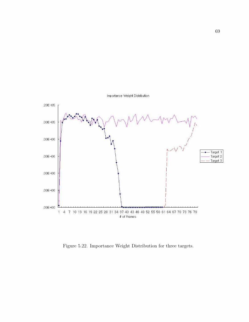
The previous subsections demonstrate tractability even in the increasing number
of targets and occlusion situations. This subsection demonstrates appearance and dis-
appearance of targets by constructing and destroying a filter. In Figure 5.22, particle
weights of Target 1 decreased as the target starts to disappear below the desk at frame
32 and a new target appears from the target 2 (plain line). The particle weights for the
new target increase as the filter is getting strong measurement supports. The important
element to note here is that dots located throughout the image represent additional filter
(background filter) and play a role in surveilling a new target that might enter the scene.
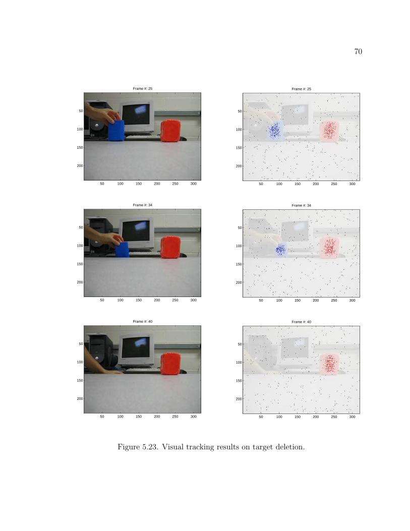
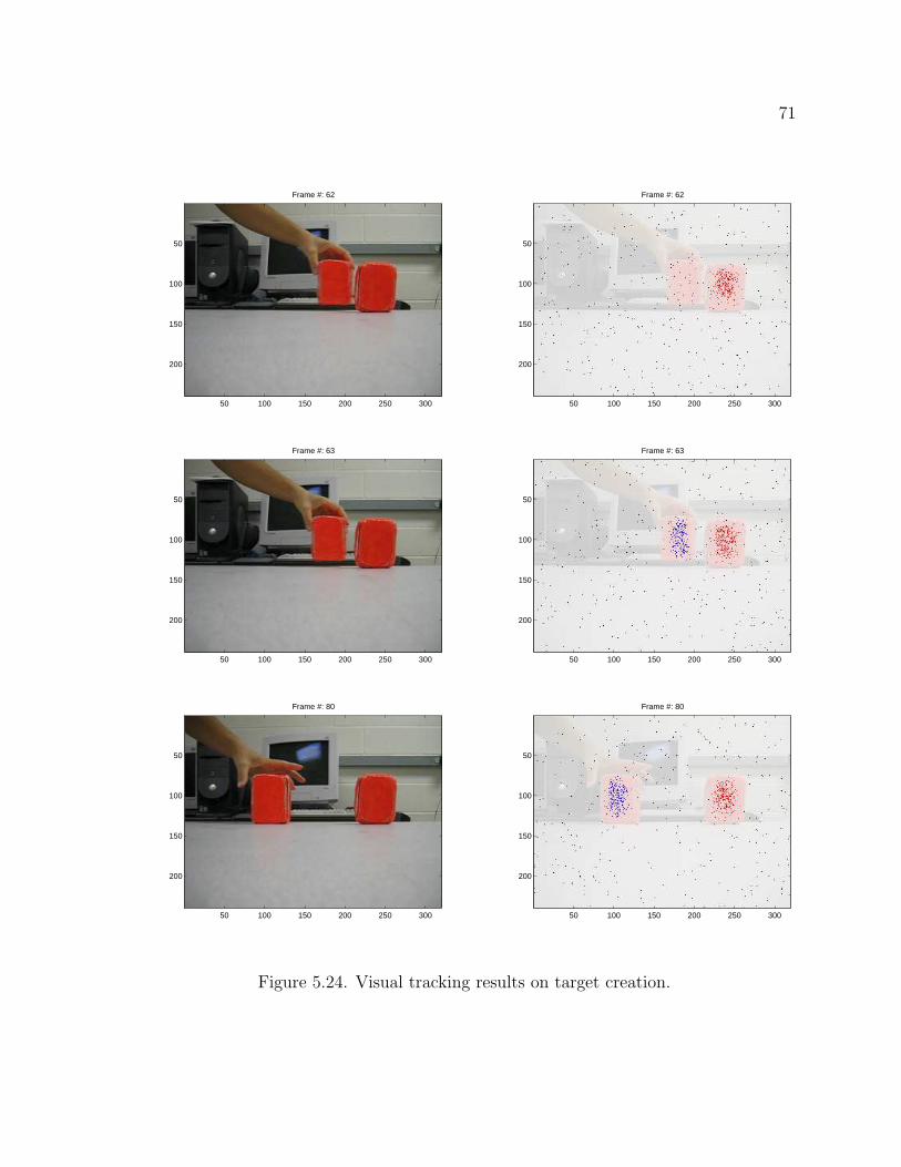
Figure 5.23 and Figure 5.24 show sequences of images where one target appears from the
foreground target. We used the same color targets because it is generally easier for a
hidden target to be detected if it has a the different color. As shown in the image figures,
the background filter detects the hidden target 3 frames after the hidden target appears
from behind the foreground target. In addition, Figure 5.22 also shows that the particle
weight distribution (target 1) is destroyed around frame 38 and new a particle weight
distribution is created around frame 59.
69
Figure 5.22. Importance Weight Distribution for three targets.
70
Frame #: 25
50 100 150 200 250 300
50
100
150
200
Frame #: 25
50 100 150 200 250 300
50
100
150
200
Frame #: 34
50 100 150 200 250 300
50
100
150
200
Frame #: 34
50 100 150 200 250 300
50
100
150
200
Frame #: 40
50 100 150 200 250 300
50
100
150
200
Frame #: 40
50 100 150 200 250 300
50
100
150
200
Figure 5.23. Visual tracking results on target deletion.
71
Frame #: 62
50 100 150 200 250 300
50
100
150
200
Frame #: 62
50 100 150 200 250 300
50
100
150
200
Frame #: 63
50 100 150 200 250 300
50
100
150
200
Frame #: 63
50 100 150 200 250 300
50
100
150
200
Frame #: 80
50 100 150 200 250 300
50
100
150
200
Frame #: 80
50 100 150 200 250 300
50
100
150
200
Figure 5.24. Visual tracking results on target creation.
72
5.3.2.4 Experiment Summaries
Figure 5.25 shows the precision of tracking one target using the standard Particle
filter and the proposed Particle filter under no collision and target disappearance. The
mean errors in both figures are similar to each other and their standard deviations are
similar as well. Figure 5.1 shows average of estimated states and their standard devia-
tions as error bars for tracking two targets and three targets after multiple runs using
standard Particle filter. Figure 5.7 shows the same information as Figure 5.1 but using
the proposed multi-target Particle filter. The results of both figures indicate that the
proposed multi-target Particle filter is capable of tracking all the targets by maintaining
low standard deviation between a true state and an estimated state, whereas the standard
Particle filter does not maintain its estimated state consistently and has a high standard
deviation at the beginning on both figures because the standard Particle filter jumps into
one target and later into the other target. Therefore, it is not suited for tracking multiple
targets.
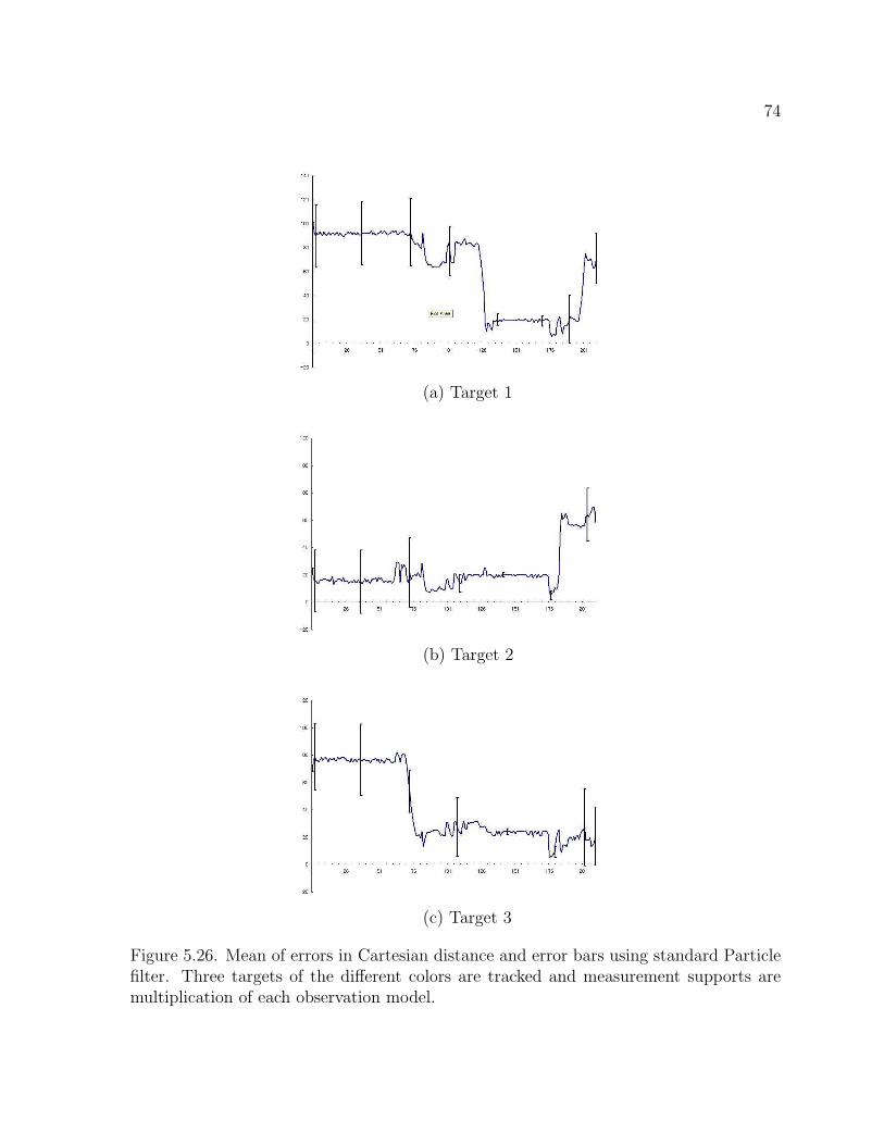
Figure 5.26 and Figure 5.14 describe evaluation of tracking three targets using the
standard Particle filter and the proposed multi-target Particle filter. Similar to the results
for tracking two targets, the proposed method is capable of tracking three targets under
occlusion situations, whereas the standard Particle filter changes a tracking target when
the targets are occluded as shown in Figure 5.26 (b) and (c) during frames 176 and 210.
73
(a) Standard Particle filter
(b) Distributed multi-target Particle filter
Figure 5.25. Mean of errors in Cartesian distance and error bars using the standardParticle filter (a) and multi-target Particle filter (b).
74
(a) Target 1
(b) Target 2
(c) Target 3
Figure 5.26. Mean of errors in Cartesian distance and error bars using standard Particlefilter. Three targets of the different colors are tracked and measurement supports aremultiplication of each observation model.
CHAPTER 6
CONCLUSIONS
A primary contribution of this thesis is its demonstration of tracking multiple tar-
gets while maintaining a computational complexity that only adds a constant factor to
a standard Particle filter. As the standard Particle filter as well as the mixture Particle
filter have problems in multi-target tracking, we proposed an extended version of the
Particle filter to remedy the problems while avoiding the complexity of a filter using a
joint distribution model. The proposed Particle filter is well suited to explain a joint
Particle distribution for visual tracking but it decreases the exponential complexity by
maintaining a distributed filter representation to a complexity that adds only a constant
factor to the standard Particle filters.
Versions of the multi-target particle filters described in Chapter 2 proposed dif-
ferent ways to make inferences about occlusions, but the proposed approach achieves
approximation to the joint observation model by projecting from particle space to image
space, while maintaining the complexity of the mixture model. The method effectively
helps tracking multiple targets robustly even under occlusion situations. The proposed
approach is evaluated through a number of experiments and demonstrated its precision
in terms of tracking targets of different colors or the same colors. In addition, we devel-
oped a filter deletion and creation approach using the joint observation model so that
the proposed approach is capable of tracking targets entering or disappearing the scene
without influencing the complexity or biasing each target distribution.
75
76
Consequently, the proposed approach strengthens the joint Particle filter by approx-
imating a new joint observation model to track multiple targets under the assumption
that the target region corresponding to each particle is monolithic, each pixel only comes
from one target, and all particles contribute equally to the particle observation without
increasing its complexity by projecting between the particle space and the image space.
REFERENCES
[1] M. Isard and J. MacCormick, “Bramble: A bayesian multiple-blob tracker.” in
ICCV, 2001, pp. 34–41.
[2] N. Wiener and E. Hopf, “On a class of singular integral equations,” 1931, p. 696.
[3] N. Wiener, Extraplation, Interpolation and smoothing of Time Series, with Engi-
neering Application. United States of America: New York: Wiley, 1949.
[4] A. N. Kolmogorov, “Stationary sequences in hilbert sapces,” p. 40, 1941.
[5] T. R. Bayes, “Essay towards solving a problem in the doctrine of chances,” pp.
370–418, 1763.
[6] J. M. Bernardo and A. F. M. Smith, Bayesian Theory. United States of America:
New York: Wiley, 1998.
[7] M. Isard and A. Blake, “Icondensation: Unifying low-level and high-level tracking
in a stochastic framework.” in ECCV (1), 1998, pp. 893–908.
[8] A. Doucet, “On sequential monte carlo sampling methods for bayesian filtering,”