Multiple Optimality Guarantees in Statistical Learning by John C Duchi A dissertation submitted in partial satisfaction of the requirements for the degree of Doctor of Philosophy in Computer Science and the Designated Emphasis in Communication, Computation, and Statistics in the Graduate Division of the University of California, Berkeley Committee in charge: Professor Michael I. Jordan, Co-chair Professor Martin J. Wainwright, Co-chair Professor Peter Bickel Professor Laurent El Ghaoui Spring 2014
Transcript
Multiple Optimality Guarantees in Statistical Learning
by
John C Duchi
A dissertation submitted in partial satisfaction of the
requirements for the degree of
Doctor of Philosophy
in
Computer Science
and the Designated Emphasis
in
Communication, Computation, and Statistics
in the
Graduate Division
of the
University of California, Berkeley
Committee in charge:
Professor Michael I. Jordan, Co-chairProfessor Martin J. Wainwright, Co-chair
Professor Peter BickelProfessor Laurent El Ghaoui
Spring 2014
Multiple Optimality Guarantees in Statistical Learning
Copyright 2014by
John C Duchi
1
Abstract
Multiple Optimality Guarantees in Statistical Learning
by
John C Duchi
Doctor of Philosophy in Computer Science
and the Designated Emphasis
in
Communication, Computation, and Statistics
University of California, Berkeley
Professor Michael I. Jordan, Co-chair
Professor Martin J. Wainwright, Co-chair
Classically, the performance of estimators in statistical learning problems is measured interms of their predictive ability or estimation error as the sample size n grows. In modernstatistical and machine learning applications, however, computer scientists, statisticians, andanalysts have a variety of additional criteria they must balance: estimators must be efficientlycomputable, data providers may wish to maintain anonymity, large datasets must be storedand accessed. In this thesis, we consider the fundamental questions that arise when tradingbetween multiple such criteria—computation, communication, privacy—while maintainingstatistical performance. Can we develop lower bounds that show there must be tradeoffs?Can we develop new procedures that are both theoretically optimal and practically useful?
To answer these questions, we explore examples from optimization, confidentiality pre-serving statistical inference, and distributed estimation under communication constraints.Viewing our examples through a general lens of constrained minimax theory, we provefundamental lower bounds on the statistical performance of any algorithm subject to theconstraints—computational, confidentiality, or communication—specified. These lower boundsallow us to guarantee the optimality of the new algorithms we develop addressing the addi-tional criteria we consider, and additionally, we show some of the practical benefits that afocus on multiple optimality criteria brings.
In somewhat more detail, the central contributions of this thesis include the following:we
• develop several new stochastic optimization algorithms, applicable to general classesof stochastic convex optimization problems, including methods that are automatically
2
adaptive to the structure of the underlying problem, parallelize naturally to attainlinear speedup in the number of processors available, and may be used asynchronously,
• prove lower bounds demonstrating the optimality of these methods,
• provide a variety of information-theoretic tools—strong data processing inequalities—useful for proving lower bounds in privacy-preserving statistical inference, communication-constrained estimation, and optimization,
• develop new algorithms for private learning and estimation, guaranteeing their opti-mality, and
• give simple distributed estimation algorithms and prove fundamental limits showingthat they (nearly) optimally trade off between communication (in terms of the numberof bits distributed processors may send) and statistical risk.
There are so many people to whom I owe credit for this thesis that I must begin with anapology: I will probably forget to mention several of you in the coming paragraphs. If I do,please forgive me, and let me know and I will be happy to buy you a beer.
My acknowledgments must begin with my advisors, my two official advisors at Berkeley,and my one surrogate advisor down at Google: Michael Jordan, Martin Wainwright, andYoram Singer. It has become clear to me that having three advisors was a necessary thing,if only for their sakes, because it kept me out of the hair of the other two while I botheredthe third. More seriously, Mike and Martin have pushed me into contact with a multitude ofdisciplines, encouraging and exemplifying a fearlessness and healthy disrespect for academicboundaries. Without them, I could not have fallen in love with as many subjects—statistics,optimization, computing—as I have, and their guidance about how to approach research,write, give talks, and cooling down my neuroses has been invaluable. They have also providedphenomenal environments for doing research, and (because of them) I have been fortunateto be surrounded constantly by other wonderful students and colleagues. Yoram has beena great mentor and friend, going on runs and bike rides with me, making sure I do notlose touch with practicality, and (hopefully) helping me develop a taste for problems at theborder of theory and practice, where one informs the other and vice versa. I hope I canmaintain the balance the three of them have modeled for me.
There are a number of other faculty who have been important to my PhD: Pieter Abbeelhas shown me what it is like to go from a graduate student to a professor and been a friendsince I was just learning to do research as an undergraduate, and his pointers helped menavigate the academic job market without panic. Ben Recht, Chris Re, and Steve Wrighthave all been wonderfully encouraging, giving feedback on papers, talks, and trying to forceme into the thinking position. I also would like to thank Daphne Koller and Gal Elidan, whoopened my eyes to the fun research gives and hard work it takes when I was an undergraduateat Stanford, and Stephen Boyd, who piqued my interest in optimization and has always beena refreshing smart aleck and kept an open door for my harassment whenever I ran into him.Fernando Pereira, with his nightly wanderings around the office in search of researchers totalk with, was a source of interesting and probing questions for all my work. Peter Bickeland Laurent El Ghaoui, who both helped by being on my thesis committee, have providedgreat feedback on several of my ideas and given good perspective.
As I wrote above, Berkeley has been an awesome environment during my PhD. The col-laborators I have had have been unequivocally phenomenal. Alekh Agarwal’s quick insightsand sharp thinking got us through a number of papers, classes, and into all sorts of funnew research areas. Lester Mackey’s patient listening and deep thinking made for wonderfulcollaborations on ranking algorithms as well as interesting conversations across a variety oftopics, and his eating was a never-ending source of entertainment. I have also been honoredto collaborate with younger students, Yuchen Zhang and Andre Wibisono, who were greatcolleagues after Alekh and Lester graduated. Andre’s mathematical insights are impressive,
vii
and I must thank Yuchen for his amazing dedication, ability to simply bulldoze any problemin front of him, and his other-worldly demeanor.
There have been a number of other great folks around the lab while I have been here:Sahand Negahban, who helped me feel not alone in my spaziness and came on some funbike rides with me (as well as providing a good sounding board to a whole pile of researchquestions), Po-Ling Loh, whose research questions and solutions were always enlightening,and Percy Liang, who showed how to really be dedicated to good work. Mike, Martin, andPeter Bartlett’s groups and the AMPLab at Berkeley, with the slew of stellar students andpost-docs coming through—Jake Abernethy (always willing to crash in a room I have at aconference), Arash Amini, Tamara Broderick, Ariel Kleiner, Simon Lacoste-Julien, GarveshRaskutti, Pradeep Ravikumar, Ameet Talwalkar (always up for a beer or some ultimate)—have been stellar. Jon Kuroda, our AMPLab jack of all trades, computer lender, and make-things-happener extraordinaire, was indispensable. And of course the EECS department IMultimate team Floppy DisKs, who remind me that in spite of our astounding nerdiness, thereare some seriously athletic folks in this department, so I should never stop running.
And now I must go back to the beginning, where everything really started, with my family.My parents, Mary and Joe, who encouraged me and gave me every learning opportunity theycould think of, set me on a trajectory of simple hunger for knowing more. With art classes,Legos, music, they seeded any creativity I might have, and (Mom) helping out with schooland (Dad) making sure I busted my tail in the swimming pool, tennis court, water polo,they showed how important a great work ethic is. I want to thank my brother, Andrew, forstill being my friend after about 12 years of abuse (I imagine your first two years were prettygood, and I think things got better when I jumped across the country when you began eighthgrade). Also, Andrew, thanks for your stories about poison oak. I’ll make sure to stay awayfrom it.
Finally, I must thank my love and wonderful wife, Emily Roberts. Marrying her, Igained a partner with an extraordinary drive to learn and listen. Emily has put up withmy conference travel, years of odd sleeping schedules and doing research until morning, andpicked up cycling (perhaps with a bit of pushing from me) so we could spend more timetogether. She taught me to backpack and will never let us spend a nice weekend inside.Emily, thank you for your love and making me happy to be with you.
1
Part I
Introduction and background
2
Chapter 1
Introduction
Modern techniques for data gathering—arising from medicine and bioinformatics [120], in-ternet applications such as web-search [86], physics and astronomical experiments [2], mobiledata gathering platforms—have yielded an explosion in the mass and diversity of data. Yetthe amount of data is no panacea; even in medium scale settings, it is challenging to identifythe best ways to analyze and make inferences from information we collect. As a consequenceof these difficulties, it is important to develop procedures that intelligently use the availabledata and trade among scarce resources: how can we balance multiple criteria—computation,communication, privacy—while maintaining statistical performance? Can we be sure we donot ask too much or make incorrect inferences?
In this thesis, we develop theoretically-motivated procedures address problems like these.Broadly, we identify desiderata that—in addition to classical metrics of statistical efficiency—we would like methods to have. In particular, we consider computational, privacy, andcommunication-based considerations as axes along which to evaluate procedures. Devel-opment along these axes has, for the most part, happened independently, as each of theconsiderations presents challenges in isolation. Given the understanding built by the sub-stantial research in optimization, information theory, computer science, and statistics andthe current challenges we face in statistical learning and data analysis, however, it is impor-tant to bring together insights from multiple fields to develop methods that trade amongstseveral criteria for improved (or optimal) performance. Progress in this direction is the goalof this thesis.
1.1 Evaluating statistical learning procedures
The classical estimation problem in statistical decision theory [118, 175] is, given an unknowndistribution P , to estimate an (unknown) parameter θ(P ) of the distribution given a sample
X drawn from the distribution. We measure the performance of a method θ according to itsexpected loss, or risk,
R(θ) := EP
[ℓ(θ(X), θ(P ))
], (1.1)
3
where ℓ(θ, θ∗) denotes a loss incurred for taking the action (or making the prediction) θ whenthe true state of the world is θ∗. The simplicity of the formulation (1.1) hides its complexity.In statistical learning scenarios [176, 50, 94], the loss may measure the expected predictionerror of a binary classifier under the distribution P . In classical statistical problems [23, 118],
we may wish to measure error ‖θ − θ∗‖22 made by θ in recovering a parameter θ∗. In thisthesis, we generally use the minimax principle, originally suggested by Wald [178], to evaluate
a procedure: for a given family P of distributions, one chooses the procedure θ minimizing
supP∈P
EP
[ℓ(θ(X), θ(P ))
]. (1.2)
There are, of course, a variety of approaches for evaluation of procedures, including Bayesianapproaches [23], but we choose to focus on minimax as a unifying principle.
The risk functional (1.1) necessarily focuses attention on performance relative to only
one metric: how well does the procedure θ minimize the loss ℓ? This central questionhas driven much of the theoretical work in statistics (and machine learning) over the lastseveral decades. But in the absence of other considerations, the risk (1.1) and minimaxprinciple (1.2) may lose practicality; there are often real-world considerations that drivedevelopment of statistical procedures, such as the costs of collecting additional observationsof the process P or establishing a controlled trial rather than simply observing the processP , questions of privacy [179, 75, 76], or the difficulty of computing particular estimators θthat may have good risk performance [174, 107, 42]. The central question of this thesis,
then, is this: how does the worst-case risk (1.2) changes when we constrain the estimator θto belong to some restricted class of procedures? Below, we outline several practical criteriathat, when considered against notions of statistical efficiency for minimizing the risk (1.1),can lead to the development of exciting new procedures and new techniques for attackingstatistical learning problems.
1.1.1 Computation
“What can be computed and how can we compute it? What is the best way to solve it?” AsJeannette Wing [181] describes it, these questions—and others like them—are the centraltenets of what she terms computational thinking. Statistical learning problems present a newflavor of problem different from standard computational tasks: there is noise inherent in theproblem (1.1), and even given infinite computational power, there often is no perfect solution,just one that attains some type of optimal error. Thus we ask a more subtle question: for agiven “computational” budget, what is the best possible error of any method? The challengein such a question is the nebulous notion of computation [10]: the Turing machine model isoften too powerful for identifying subtle differences in computation, and other definitions ofcomputation are often more specialized.
We are not the first to ask this type of question, and several authors have attacked sim-ilar problems, beginning with the work of Valiant [174] on Probably Approximately Correct
4
(PAC) learning, which separates concepts that can be learned with polynomial sample sizefrom those that cannot. More recent work building out of this has often arrived at thesometimes counterintuitive result that more data (larger problems) yields faster algorithms.Bottou and Bousquet [30] and Shalev-Shwartz et al. [162, 161] describe settings in whichincreased data set sizes allow faster learning of classifiers. Berthet and Rigollet [24] studycomputation time/data tradeoffs in sparse principal component analysis, and work by Chan-drasekaran and Jordan [42] show how the complexity of convex sets relates to estimationperformance in Gaussian sequence models. In another line of work, Agarwal, Bartlett, andDuchi [5] study model selection under computational constraints, where they force proce-dures to operate within a given abstract computational budget.
To give ourselves a model of computation that is both practically relevant and theo-retically tractable, in this thesis, we identify optimization complexity with computationalcomplexity, using the tools of information-based complexity developed by Nemirovski andYudin [134] and Traub et al. [169] (see also the introductory survey by Traub and Werschulz[168], the book of Plaskota [144], and the paper of Agarwal et al. [6], which is particularlyrelevant to this thesis). In these settings, we usually assume we are minimizing a function
f(θ) := E[F (θ;X)]
over θ ∈ Θ ⊂ Rd, and we treat the computation of an instantaneous loss F (θ;X) or gradientevaluation ∇θF (θ;X) as our computational unit. Given the prevalence of optimizationalgorithms based on first-order (gradient) information [136, 32, 98, 134], this focus is bothnatural and practically motivated. We may then study—for different classes of domains Θ,types of losses F , and families of probability distributions P according to which the data Xare generated—the complexity of optimization.
In addition to asking about the fundamental complexity of optimization in terms of ze-roth or first-order information, given the modern development of multi-core and distributedcomputing infrastructure, it is also important to study aspects of parallel, asynchronous,and distributed computation [26, 79, 14, 33, 49]. To what extent can we maintain opti-mality of optimization procedures while leveraging parallel computation? We address suchquestions in this thesis as well, giving algorithms that maintain both optimal complexity—in terms of their number of gradient or function evaluations—while running in parallel orasynchronously.
1.1.2 Privacy
As the scale of datasets—with the concomitant amount of information we collect aboutindividuals—increases, maintaining anonymity and privacy has become more important.While the maintaining privacy is an old issue, dating at least to Warner’s 1960s work onrandomized response and survey sampling [179], it has become clear that modern data col-lection poses new risks of disclosure. For example, Homer et al. [99] recently showed it ispossible to identify the presence of individual genotypes in high-density SNP arrays, leading
5
to the removal of some publicly available genomics data [83]. A major challenge in statisticalinference has thus become that of characterizing and balancing statistical utility with theprivacy of individuals from whom we obtain data [63, 64, 76].
In the large body of research on privacy and statistical inference [e.g., 179, 75, 63, 64, 76],a major focus has been on the problem of reducing disclosure risk: the probability that amember of a dataset can be identified given released statistics of the dataset. The literaturehas stopped short, however, of providing a formal treatment of disclosure risk that wouldpermit decision-theoretic tools to be used in characterizing tradeoffs between the utility ofachieving privacy and the utility associated with an inferential goal. Recently, a formaltreatment of disclosure risk known as “differential privacy” has been proposed by Dworkand colleagues and studied in the cryptography, database and theoretical computer scienceliteratures [68, 65]. Differential privacy has strong semantic privacy guarantees that makeit a good candidate for declaring a statistical procedure private, and it has been the focusof a growing body of recent work [65, 74, 91, 180, 164, 44, 105]. Direct connections betweenstatistical risk (1.1) and privacy, however, have been somewhat more challenging to make;with modern issues in data collection, however, it is becoming more important to understandquantitative tradeoffs between privacy and statistical efficiency.
1.1.3 Communication
While computational considerations are important for the development of estimation and in-ferential procedures, the scale of modern datasets often necessitates distributed storage andcomputation [86]. Perhaps even more saliently, computer processing speeds are beginningto hit fundamental physical limits [79], and, as Fuller and Millett [79] point out in a surveyfor the National Academy of Sciences, our only “known hope” for continued improvement incomputational performance is to leverage parallel and distributed computing. The relativeexpense of communication with respect to computation, however, makes inter-processor orinter-machine communication an especially important resource and measure of the perfor-mance of algorithms [14, 79]. Moreover, the rates at which communication costs improveare slower than those of other computing tasks, so communication is becoming both moreimportant—due to the rise in parallelism and large datasets—and its relative costs are alsoincreasing. Additionally, connecting the tools of information theory [47], which allow usto describe the fundamental limits of communication and storage, with statistical inferenceproblems has been somewhat challenging [89]. It is thus important to understand funda-mental limits in distributed statistical estimation problems and to discover new proceduresthat attain these limits.
1.2 Thesis goals and contributions
The focus of this thesis is to develop, via examples in stochastic approximation, privacy-preserving inference, and communication-constrained estimation, approaches for designing
6
and analyzing methods whose performance is measured along multiple axes. Using classi-cal statistical minimax theory as our starting point, we introduce a notion of constrainedminimax risk, and we using this measure of performance, we develop fundamental lowerbounds and procedures attaining them for a variety of problems. This development requiresa two-pronged approach, where we show the fundamental hardness of problems—giving lowerbounds, leveraging ideas from optimization, information theory, and statistics—and deriveefficient algorithms achieving these bounds. By attacking problems from both sides, it is pos-sible to gain deeper insights into the underlying difficulties, relaxations and circumventionsof those difficulties, and essential structures of the problems being solved. Building on theseinsights, we can derive algorithms that trade amongst a multitude of criteria for improvedperformance, yielding more efficient procedures for real large-scale statistical, learning, andoptimization problems.
In particular, the goals of this thesis are to
(1) Introduce a notion of minimax risk for estimators constrained by particular resource (orother) requirements and to develop tools for proving fundamental lower bounds on thesenotions of risk, and
(2) Develop new procedures for different types of constraints, focusing on computational(via optimization), confidentiality, and communication-based constraints.
More specifically, the central contributions of the thesis are the following:
• We review and extend several techniques for proving minimax lower bounds, developinga few finer-grained information-theoretic inequalities that allow easier proofs of manylower bounds
• We show new ways the performance of stochastic optimization algorithms depends onthe geometry underlying the problem, and we show how to give algorithms that areoptimal—and adaptive—to the underlying problem structure
• We show how the use of dual averaging algorithms allows (nearly) completely asyn-chronous optimization schemes whose performance improves linearly with the numberof processors in parallel computing environments, as long as data obeys certain sparsityrestrictions
• We develop randomized smoothing techniques that (i) yield optimal algorithms for non-smooth (sub)gradient-based optimization, even in parallel computing environments,and (ii) extend these to zeroth order optimization schemes, providing new optimalalgorithms (as well as guarantees of their optimality)
• We develop quantitative data processing inequalities that allow the application of ourinformation-theoretic techniques to privacy-preserving data analyses, providing newfundamental lower bounds on the performance of procedures that maintain privacy inestimation problems
7
• We provide new algorithms that attain the fundamental limits for privacy-preservingestimation in “local-privacy” settings where data providers do not even trust the datacollector
• We review recent low-communication optimization and estimation schemes, and weadapt our information-theoretic tools (again based on new data-processing inequalities)to prove fundamental limits on communication-constrained estimation procedures.
A common theme in all of our algorithms is that they exploit problem structure—the sta-tistical properties and the noise inherent to the problem—for more efficient methods. Inthe stochastic optimization case, this comes in the form of adding additional noise that isof lower order than that already in the problem, either via randomized smoothing or asyn-chrony, and enjoying consequent speedups. In the privacy case, this comes in the form ofdirectly adding noise to data to protect confidentiality, while using the statistical structureof the data to avoid adding more noise than necessary. In the low-communication case, thisconsists of observing that averaging independent distributed solutions is nearly sufficient foroptimal solution of many statistical problems, because each processor’s local solution is sim-ply a noisy approximation to the truth, rather than the solution to an adversarially chosenproblem. In a sense, the thesis simply studies what good a little noise can do.
1.3 Organization of the thesis and previously
published work
Several portions of this thesis are based on joint work of mine with collaborators, which Idescribe (briefly) here, in addition to outlining the rest of the thesis. Part I of this thesis pro-vides some background on minimax theory, setting up (at an abstract level) the constrainedminimax problem by which we evaluate our procedures in Chapter 2. Much of the materialin the chapter is classical, though some of it is based on joint work with Martin Wainwrightand Michael Jordan [51, 59].
In Part II of the thesis, we focus on stochastic optimization problems, investigatingcomputational limits (via information-based complexity) as well as distributed and asyn-chronous optimization techniques. Chapters 3 and 4 study adaptive optimization schemesand single-processor optimality guarantees (Chapter 3) and characteristics of data that allowasynchronous parallel algorithms (Chapter 4). They contain some new material and somebased on joint work with Michael Jordan and Brendan McMahan [58], which builds off ofearlier research performed jointly with Elad Hazan and Yoram Singer [53]. Chapter 5 studiesrandomized smoothing techniques to develop optimal optimization schemes for non-smoothproblems and is based on work with Peter Bartlett and Martin Wainwright [55], while Chap-ter 6 extends these randomized smoothing ideas to attack optimization problems where onlyzeroth order (function value) information is available, providing new (optimal) schemes and
8
fundamental lower bounds for such problems. It is based on work with Michael Jordan,Andre Wibisono, and Martin Wainwright [61].
Part III of the thesis is on tradeoffs between privacy and statistical utility, studying theeffects of imposing local privacy on convergence rates for statistical estimators, and buildsout of joint work with Michael Jordan and Martin Wainwright [60, 59].
Finally, Part IV of the thesis studies some effects of communication on distributed esti-mators. Chapter 9 reviews simple distributed estimation algorithms developed jointly withYuchen Zhang and Martin Wainwright [189], and in Chapter 10, we develop informationtheoretic tools to exhibit the fundamental limits and tradeoffs between statistical efficiencyand inter-machine communication. This final chapter is based off of joint work with YuchenZhang, Michael Jordan, and Martin Wainwright [62].
1.4 Notation
Before proceeding to the thesis proper, we define notation and terminology that we commonlyuse; our settings are essentially standard. Throughout, we use R to denote the real numbersand N = 1, 2, . . . to denote the counting numbers.
Asymptotic notation We use standard asymptotic notation throughout the thesis. Inparticular, we use O(·), Ω(·), Θ(·), and o(·). Formally, for real-valued sequences ann∈N andbnn∈N, we say that an = O(bn) if there exists a constant c < ∞ and an N ∈ N such thatan ≤ cbn for all n ≥ N . Similarly, we say an = Ω(bn) if bn = O(an), that is, there exists aconstant c > 0 and N ∈ N such that an ≥ cbn for n ≥ N , and an = Θ(bn) if an = O(bn) andan = Ω(bn). We say an = o(bn) if |an|/|bn| → 0 as n → ∞. We use the notation an . bn todenote an = O(bn), and an ≪ bn to denote an = o(bn), meaning that “an is at most on theorder of bn” and “an is significantly smaller than bn.” In general, unless otherwise specified,our asymptotic notation will hide only numerical constants that do not depend on problemparameters and will apply with N = 1.
Statistical notation We require standard statistical notation throughout the thesis. Givena sequence of random variables Xn and another random variable (or constant) Y all tak-ing values in a metric space X with distance ρ, we say that Xn converges in probabilityto Y , meaning that Xn
p→ Y , if for all ǫ > 0 we have P(ρ(Xn, Y ) > ǫ) → 0 as n → ∞.We say that Xn converges in distribution to Y (or, if Y is distributed according to P , de-noted Y ∼ P , that Xn converges in distribution to P ) if for all bounded and continuousfunctions f : X → R we have E[f(Xn)] → E[f(Y )] as n → ∞. See, for example, the Port-manteau Theorem [e.g. 175] for equivalent definitions. We use statistical big-O notation aswell (see, for example, Lehmann and Casella [118]). Given two sequences of random vari-ables or vectors Xn and Yn on spaces X and Y with norms ‖·‖X and ‖·‖Y , we say thatXn = OP (Yn) if for each ǫ > 0, there exists a constant C(ǫ) and N ∈ N such that n ≥ N
9
implies P(‖Xn‖X ≥ C(ǫ) ‖Yn‖Y) ≤ ǫ. A random variable X is sub-Gaussian [e.g. 36] withparameter σ2 if for all λ ∈ R, we have E[exp(λX)] ≤ exp(λ2σ2/2).
Given two probability distributions P and Q on a space X , each assumed absolutelycontinuous with respect to an underlying measure µ with densities p and q respectively,1 theKL-divergence between P and Q is
Dkl (P ||Q) =∫
Xp(x) log
p(x)
q(x)dµ(x).
Given a discrete random variable X defined on a space X with probability mass func-tion (p.m.f.) p, its (Shannon) entropy [47] is H(X) := −∑x∈X p(x) log p(x). The condi-tional entropy of X given Y , where X and Y have joint p.m.f. p(x, y), is H(X | Y ) :=−∑x,y p(x, y) log p(x | y). Given random variables X and Y with marginal distributions PXand PY , respectively, and joint PX,Y , the mutual information between X and Y is
I(X;Y ) :=
∫
X×YpX,Y (x, y) log
pX,Y (x, y)
pX(x)pY (y)dµ(x, y)
= EPX[Dkl (PY (· | X)||PY (·))] =
∫
XDkl (PY (· | X = x)||PY (·)) dPX(x),
where µ is a measure assumed to dominate PX,Y and p is the density of P with respect toµ. Throughout we use log base-e for our entropy and information theoretic calculations. Ifσ(X ) denotes the σ-field on X , the total variation distance between two distributions P andQ defined on (X , σ(X )) is
‖P −Q‖TV := supS∈σ(X )
|P (S)−Q(S)| = 1
2
∫
X|p(x)− q(x)|dµ(x).
We use N(θ,Σ) to denote the normal distribution with mean θ and covariance matrix Σand Laplace(κ) to denote the Laplace distribution with inverse shape parameter κ, that is,density p(x) ∝ exp(−κ|x|).
Analytic, matrix, and vector notation For vectors x ∈ Rd, we use ℓp to denote the
usual p-norms ‖x‖p = (∑d
j=1 |xj|p)1p , where ‖x‖∞ = maxj |xj|. The ℓ2-operator norm of a
matrix A ∈ Rd1×d2 is its maximum singular value, defined by
|||A||| = |||A|||2 := supv∈Rd2 ,‖v‖2≤1
‖Av‖2 .
We use γi(A) to denote the ith singular value of A, and ‖A‖Fr to denote its Frobenius norm.We let 〈·, ·〉 denote the standard inner product on Rd (or whatever space is being used), andgiven a norm ‖·‖ on Rd, the dual norm ‖·‖∗ is given by
‖y‖∗ = supx∈Rd
〈x, y〉 : ‖x‖ ≤ 1 .1This is no loss of generality, as we may take µ = 1
2P + 1
2Q
10
A set X ⊂ Rd is convex if x, y ∈ X implies that λx + (1 − λ)y ∈ X for all λ ∈ [0, 1]. Afunction f is convex if its domain dom f is convex, and f(λx+(1−λ)y) ≤ λf(x)+(1−λ)f(y)for all x, y ∈ dom f and λ ∈ [0, 1]. We denote the subgradient set of f at a point x by
∂f(x) := g ∈ Rd : f(y) ≥ f(x) + 〈g, y − x〉 for all y ∈ Rd.
For shorthand, we let ‖∂f(x)‖ = supg∈∂f(x) ‖g‖. We make the standard assumption [98, 152]that f(y) = +∞ for all y 6∈ dom f for convex f . To avoid pathologies, any convex function fin this thesis is assumed to be sub-differentiable over all of dom f . The Euclidean projectionof a point y onto a closed convex set C is
ΠC(y) := argminx∈C
‖x− y‖22
.
For any function f and a norm ‖·‖, we say that f isM -Lipschitz continuous with respectto the norm ‖·‖ over X if
|f(x)− f(y)| ≤M ‖x− y‖ for all x, y ∈ X .
Similarly, for f differentiable on a set X , we say that ∇f is L-Lipschitz continuous withrespect to a norm ‖·‖ (with associated dual norm ‖·‖∗) if
‖∇f(x)−∇f(y)‖∗ ≤ L ‖x− y‖ for all x, y ∈ X .
We let ⊗ denote the Kronecker product, and for a pair of vectors u, v, we define the outerproduct u ⊗ v = uv⊤. For a three-times differentiable function f : Rd → R, we denote thethird derivative tensor by ∇3f , so that for each x ∈ dom f the operator ∇3f(x) : Rd×d → Rd
is linear and satisfies the relation
[∇3f(x)(v ⊗ v)
]i=
d∑
j,k=1
(∂3
∂xi∂xj∂xkf(x)
)vjvk.
Miscellaneous notation We denote the indicator function of an event E by 1 E, whichis 1 if E occurs (or is true) and 0 otherwise. For an integer n, the notation [n] denotes theset of integers 1, . . . , n. We let ∨ and ∧ denote maximum and minimum, respectively, sothat a ∨ b = maxa, b and a ∧ b = mina, b.
11
Chapter 2
Minimax rates of convergence
Understanding the fundamental limits of estimation and optimization procedures is impor-tant for a multitude of reasons. Indeed, developing bounds on the performance of procedurescan give complementary insights. By exhibiting fundamental limits of performance (perhapsover restricted classes of estimators), it is possible to guarantee that an algorithm we havedeveloped is optimal, so that searching for estimators with better statistical performancewill have limited returns, though searching for estimators with better performance in othermetrics may be interesting. Moreover, exhibiting refined lower bounds on the performanceof estimators can also suggest avenues for developing alternative, new optimal estimators;lower bounds need not be a fully pessimistic exercise.
In this chapter, we define and then discuss techniques for lower-bounding the minimaxrisk, giving three standard techniques for deriving minimax lower bounds that have provenfruitful in a variety of statistical learning problems [188]. In addition to reviewing thesestandard techniques—the Fano, Assouad, and Le Cam methods—we also present a fewsimplifications and extensions that may make them more “user friendly.”
2.1 Basic framework and minimax risk
Our first step here is to establish the minimax framework we use throughout the thesis.Depending on the problem we study, we use either minimax risk or what is known as minimaxexcess risk to evaluate optimality of our estimation procedures. Our setting is essentiallystandard, and we refer to references [188, 185, 173] for further background. Let us beginby defining the standard minimax risk, deferring temporarily our discussion of minimaxexcess risk. Throughout, we let P denote a class of distributions on a sample space X ,and let θ : P → Θ denote a function defined on P , that is, a mapping P 7→ θ(P ). Thegoal is to estimate the parameter θ(P ) based on observations Xi drawn from the (unknown)distribution P .
The space Θ in which the parameter θ(P ) takes values depends on the underlying statis-tical problem; as an example, if the goal is to estimate the univariate mean θ(P ) = EP [X],
12
we have Θ ⊂ R. To evaluate the quality of an estimator θ, we let ρ : Θ × Θ denote a(semi)metric on the space Θ, which we use to measure the error of an estimator for theparameter θ, and let Φ : R+ → R+ be a non-decreasing function with Φ(0) = 0 (for example,Φ(t) = t2).
In classical settings, the statistician is given direct access to i.i.d. observations Xi drawnaccording to some P ∈ P . Based on these Xi, the goal is to estimate the unknown
parameter θ(P ) ∈ Θ , and an estimator θ is a measurable function θ : X n → Θ. We then
assess the quality of the estimate θ(X1, . . . , Xn) in terms of the risk
EP
[Φ(ρ(θ(X1 . . . , Xn), θ(P ))
)].
For instance, for a univariate mean problem with ρ(θ, θ′) = |θ− θ′| and Φ(t) = t2, this risk isthe mean-squared error. Of course, for any fixed distribution P , it is easy to estimate θ(P ):simply return θ(P ), which will have minimal risk. It is thus important to ask for a moreuniform notion of risk, which leads to the minimax principle, first suggested by Wald [178],
which is to choose the estimator (measurable function) θ minimizing the maximum risk
supP∈P
EP
[Φ(ρ(θ(X1 . . . , Xn), θ(P ))
)].
An optimal estimator for this metric then gives the minimax risk, which is defined as
Mn(θ(P),Φ ρ) := infθsupP∈P
EP
[Φ(ρ(θ(X1, . . . , Xn), θ(P ))
)], (2.1)
where we take the supremum (worst-case) over distributions P ∈ P , and the infimum is
taken over all estimators θ.In some scenarios, we study a slightly different notion of risk, which is more appropriate
for some learning and optimization problems. In these settings, we assume there exists someloss function ℓ : Θ×X → R, where for an observation x ∈ X , the value ℓ(θ; x) measures theinstantaneous loss associated with using θ as a predictor. In this case, we define the risk
RP (θ) := EP [ℓ(θ;X)] =
∫
Xℓ(θ; x)dP (x) (2.2)
as the expected loss of the parameter vector θ. For a (potentially random) estimator θ :X n → Θ given access to a sample X1, . . . , Xn, we may define the associated maximumexcess risk for the family P by
supP∈P
EP
[RP (θ(X1, . . . , Xn))
]− inf
θ∈ΘR(θ)
,
where the expectation is taken over Xi and any randomness in the procedure θ. This expres-sion captures the difference between the (expected) risk performance of the procedure θ and
13
the best possible risk, available if the distribution P were known ahead of time. The mini-max excess risk, defined with respect to the loss ℓ, domain Θ, and family P of distributions,is then defined by the best possible maximum excess risk,
Mn(Θ,P , ℓ) := infθsupP∈P
EP
[RP (θ(X1, . . . , Xn))
]− inf
θ∈ΘRP (θ)
, (2.3)
where the infimum is taken over all estimators θ : X n → Θ and the risk RP is implicitlydefined in terms of the loss ℓ. The techniques for providing lower bounds for the minimaxrisk (2.1) or the excess risk (2.3) are essentially identical; we focus for the remainder of thissection on techniques for providing lower bounds on the minimax risk.
The minimax risk (2.1) is well-studied, beginning with work of Wald [178] and continuingthrough a multitude of researchers; important references include the books by Le Cam [115]and Ibragimov and Has’minskii [101], the papers of Birge [27], Yu [188], and Yang andBarron [185], and the recent introductory survey of Tsybakov [173] provides an overviewof minimax techniques in non-parametric estimation. In this thesis, however, we study avariant of the minimax risk where we constrain our estimators θ to belong to a particularclass C of estimators. In particular, letting C denote a subset of the (measurable) functions
θ : X n → Θ, we define the constrained minimax risk
Mn(θ(P),Φ ρ, C) := infθ∈C
supP∈P
EP
[Φ(ρ(θ(X1, . . . , Xn), θ(P ))
)]. (2.4)
In this thesis, we take a few steps—via examples in optimization, communication-constrainedestimation, and privacy-preserving statistical inference—toward the study of the object (2.4).
While the change to a constrained class of estimators may appear at first glance to besuperficial, it will become clear that study of such constrained estimators is both challengingand can yield new, interesting procedures. The constrained minimax principle (2.4) is thus,essentially, the driving force of this research. Indeed, in Part II of the thesis, we show howsuch constraints and an understanding of minimax lower bounds can give rise to new andefficient algorithms for optimization. In Part III, we develop techniques for proving minimaxlower bounds for statistical estimation when providers of the data wish to guarantee that theirdata is private, and we give corresponding new (optimal) procedures for private estimation.Finally, in Part IV, we analyze a few simple procedures for distributed statistical estimation,showing that they in fact enjoy optimality guarantees both in statistical and communication-theoretic senses.
2.2 Methods for lower bounds: Le Cam, Assouad,
and Fano
There are a variety of techniques for providing lower bounds on the minimax risk (2.1) (and,by extension, (2.4)). Each of them transforms the maximum risk by lower bounding it via a
14
Bayesian problem (e.g. [101, 115, 118]), then proving a lower bound on the performance ofall possible estimators for the Bayesian problem. In particular, let Pv ⊂ P be a collectionof distributions in P indexed by v and π be any probability mass function over v. Then forany estimator θ, the maximum risk has lower bound
supP∈P
EP
[Φ(ρ(θ(X1, . . . , Xn), θ(P )))
]≥∑
v
π(v)EPv
[Φ(ρ(θ(X1, . . . , Xn), θ(Pv)))
].
While trivial, this lower bound serves as the departure point for each of the subsequenttechniques for lower bounding the minimax risk.
2.2.1 From estimation to testing
A standard first step in proving minimax bounds is to reduce the estimation problem toa testing problem [188, 185, 173]. We use two types of testing problems: one a multiplehypothesis test, the second based on multiple binary hypothesis tests. We begin with thesimpler of the two. Given an index set V of finite cardinality, consider a family of distributionsPvv∈V contained within P . This family induces a collection of parameters θ(Pv)v∈V ; itis a 2δ-packing in the ρ-semimetric if
ρ(θ(Pv), θ(Pv′)) ≥ 2δ for all v 6= v′.
We use this family to define the canonical hypothesis testing problem:
• first, nature chooses V according to the uniform distribution over V ;
• second, conditioned on the choice V = v, the random sample X = (X1, . . . , Xn) isdrawn from the n-fold product distribution P n
v .
Given the observed sample X, the goal is to determine the value of the underlying index v.We refer to any measurable mapping Ψ : X n → V as a test function. Its associated errorprobability is P(Ψ(X1, . . . , Xn) 6= V ), where P denotes the joint distribution over the randomindex V and X. The classical reduction from estimation to testing [e.g., 173, Section 2.2]guarantees that the minimax error (2.1) has lower bound
Mn(θ(P),Φ ρ) ≥ Φ(δ) infΨ
P(Ψ(X1, . . . , Xn) 6= V ), (2.5)
where the infimum ranges over all testing functions.To see this result, fix an arbitrary estimator θ. Suppressing dependence on X throughout
the derivation, first note that it is clear that for any fixed θ, we have
E[Φ(ρ(θ, θ))] ≥ E[Φ(δ)1
ρ(θ, θ) ≥ δ
]≥ Φ(δ)P(ρ(θ, θ) ≥ δ),
15
θθv
θv′ 2δ
Figure 2.1. Example of a 2δ-packing of a set. The estimate θ is contained in at most oneof the δ-balls around the points θv.
where the final inequality follows because Φ is non-decreasing. Now, let us define θv = θ(Pv),so that ρ(θv, θv′) ≥ 2δ for v 6= v′. By defining the testing function
Ψ(θ) := argminv∈V
ρ(θ, θv),
breaking ties arbitrarily, we have that ρ(θ, θv) < δ implies that Ψ(θ) = v because of the tri-angle inequality and 2δ-separation of the set θvv∈V . Equivalently, for v ∈ V , the inequalityΨ(θ) 6= v implies ρ(θ, θv) ≥ δ. (See Figure 2.1.) By averaging over V , we find that
supP
P(ρ(θ, θ(P )) ≥ δ) ≥ 1
|V|∑
v∈VP(ρ(θ, θ(Pv)) ≥ δ | V = v) ≥ 1
|V|∑
v∈VP(Ψ(θ) 6= v | V = v).
Taking an infimum over all tests Ψ : X n → V gives inequality (2.5).The remaining challenge is to lower bound the probability of error in the underlying
multi-way hypothesis testing problem, which we do by choosing the separation δ to trade offbetween the loss Φ(δ) (large δ increases the loss) and the probability of error (small δ, andhence separation, makes the hypothesis test harder). Usually, one attempts to choose thelargest separation δ that guarantees a constant probability of error. There are a variety oftechniques for this, and we present three: Le Cam’s method, Fano’s method, and Assouad’smethod, including extensions of the latter two to enhance their applicability.
2.2.2 Le Cam’s method
Le Cam’s method, in its simplest form, provides lower bounds on the error in simple binaryhypothesis testing testing problems. That is, it is applicable when there are two values v, v′
16
in V . It is a standard result [115, 188, Lemma 1] that the total variation distance has thevariational representation
for any two distributions P,Q, where the first infimum is taken over all non-negative mea-surable functions and the second over all tests. Thus, when V = v with probability 1
2and v′
with probability 12, we have
infΨ
P (Ψ(X1, . . . , Xn) 6= V ) =1
2− 1
2‖P n
v − P nv′‖TV . (2.7)
In particular, this lower bound implies that for any pair of family P of distributions forwhich there exists a pair P1, P2 ∈ P satisfying ρ(θ(P1), θ(P2)) ≥ 2δ, then
Mn(θ(P),Φ ρ) ≥ Φ(δ)
[1
2− 1
2‖P n
1 − P n2 ‖TV
]. (2.8)
Example: Bernoulli mean estimation As an illustrative application of Le Cam’smethod, consider the problem of estimating the mean θ ∈ [−1, 1] of a ±1-valued Bernoullidistribution under the squared error loss, where Xi ∈ −1, 1. In this case, by fixing someδ > 0, we set V = −1, 1, and we define Pv so that
Pv(X = 1) =1 + vδ
2and Pv(X = −1) = 1− vδ
2,
whence we see that the mean θ(Pv) = δv. Using the metric ρ(θ, θ′) = |θ − θ′| and lossΦ(δ) = δ2, we have separation 2δ of θ(P−1) and θ(P1). Thus, via Le Cam’s method (2.8), wehave that
Mn(Bernoulli([−1, 1]), (·)2) ≥1
2δ2(1−
∥∥P n−1 − P n
1
∥∥TV
).
We would thus like to upper bound ‖P n−1 − P n
1 ‖TV as a function of the separation δ andsample size n; we do this using Pinsker’s inequality [e.g. 47]. Indeed, we have
∥∥P n−1 − P n
1
∥∥2TV≤ 1
2Dkl
(P n−1||P n
1
)=n
2Dkl (P−1||P1) =
n
2δ log
1 + δ
1− δ .
Noting that δ log 1+δ1−δ ≤ 3δ2 for δ ∈ [0, 1/2], we obtain that ‖P n
−1 − P n1 ‖TV ≤ δ
√3n/2 for
δ ≤ 1/2. In particular, we can guarantee a high probability of error in the associatedhypothesis testing problem (recall inequality (2.7)) by taking δ = 1/
√6n; this guarantees
‖P n−1 − P n
1 ‖TV ≤ 12. We thus have the minimax lower bound
Mn(Bernoulli([−1, 1]), (·)2) ≥1
2δ2(1− 1
2
)=
1
24n,
which is sharp to within constant factors.
17
2.2.3 Fano’s method
Fano’s method, originally proposed by Has’minskii [92] for providing lower bounds in non-parametric estimation problems, gives a somewhat more general technique than Le Cam’smethod, and it applies when the packing set V has cardinality larger than two. Themethod has played a central role in minimax theory, beginning with the pioneering workof Has’minskii and Ibragimov [92, 101]. More recent work following this initial push contin-ues to the present day (e.g. [27, 188, 185, 28, 148, 85, 37]).
We begin by stating Fano’s inequality, which provides a lower bound on the error ina multi-way hypothesis testing problem. Let V be a random variable taking values in afinite set V with cardinality |V| ≥ 2. If we define the binary entropy function h2(p) =−p log p− (1− p) log(1− p), Fano’s inequality takes the following form [e.g. 47, Chapter 2]:
Lemma 2.1 (Fano). For any Markov chain V → X → V , we have
h2(P(V 6= V )) + P(V 6= V ) log(|V| − 1) ≥ H(V | V ). (2.9)
A standard simplification of Lemma 2.1 is to note that h2(p) ≤ log 2 for any p ∈ [0, 1], sothat if V is uniform on the set V and hence H(V ) = log |V|, then for a sample X, we havethe testing lower bound
infΨ
P(Ψ(X) 6= V ) ≥ 1− I(V ;X) + log 2
log |V| (2.10)
in the canonical hypothesis testing problem from Section 2.2.1.While the testing lower bound (2.10) is sufficient for proving lower bounds for many
estimation problems, for the sharpest results it sometimes requires a somewhat delicate con-struction of a well-separated packing (e.g. [37, 60]). To that end, we also provide extensionsof inequalities (2.9) and (2.10) that more directly yield bounds on estimation error, allowingmore direct and simpler proofs of a variety of minimax lower bounds (see also reference [51]).
More specifically, suppose that the distance function ρV is defined on V , and we areinterested in bounding the estimation error ρV(V , V ). We begin by providing analogues ofthe lower bounds (2.9) and (2.10) that replace the testing error with the tail probability
P(ρV(V , V ) > t). By Markov’s inequality, such control directly yields bounds on the expec-
tation E[ρV(V , V )]. As we show in the sequel and in chapters to come, these distance-basedFano inequalities allow more direct proofs of a variety of minimax bounds without the needfor careful construction of packing sets or metric entropy calculations as in other arguments.
We begin with the distance-based analogue of the usual discrete Fano inequality inLemma 2.1. Let V be a random variable supported on a finite set V with cardinality |V| ≥ 2,and let ρ : V × V → R be a function defined on V × V . In the usual setting, the function ρis a metric on the space V , but our theory applies to general functions. For a given scalart ≥ 0, the maximum and minimum neighborhood sizes at radius t are given by
Nmaxt := max
v∈Vcardv′ ∈ V | ρ(v, v′) ≤ t and Nmin
t := minv∈Vcardv′ ∈ V | ρ(v, v′) ≤ t .
(2.11)
18
Defining the error probability Pt = P(ρV(V , V ) > t), we then have the following generaliza-tion of Fano’s inequality:
Proposition 2.1. For any Markov chain V → X → V , we have
h2(Pt) + Pt log|V| −Nmin
t
Nmaxt
+ logNmaxt ≥ H(V | V ). (2.12)
Before proving the proposition, which we do in Section 2.4.1, it is informative to notethat it reduces to the standard form of Fano’s inequality (2.9) in a special case. Supposethat we take ρV to be the 0-1 metric, meaning that ρV(v, v
′) = 0 if v = v′ and 1 otherwise.
Setting t = 0 in Proposition 2.1, we have P0 = P[V 6= V ] and Nmin0 = Nmax
0 = 1, whenceinequality (2.12) reduces to inequality (2.9). Other weakenings allow somewhat clearerstatements (see Section 2.4.2 for a proof):
Corollary 2.1. If V is uniform on V and (|V| −Nmint ) > Nmax
t , then
P(ρV(V , V ) > t) ≥ 1− I(V ;X) + log 2
log |V|Nmax
t
. (2.13)
Inequality (2.13) is the natural analogue of the classical mutual-information based form ofFano’s inequality (2.10), and it provides a qualitatively similar bound. The main differenceis that the usual cardinality |V| is replaced by the ratio |V|/Nmax
t . This quantity serves as arough measure of the number of possible “regions” in the space V that are distinguishable—that is, the number of subsets of V for which ρV(v, v
′) > t when v and v′ belong to differentregions. While this construction is similar in spirit to the usual construction of packing setsin the standard reduction from testing to estimation (cf. Section 2.2.1), our bound allows usto skip the packing set construction. We can directly compute I(V ;X) where V takes valuesover the full space, as opposed to computing the mutual information I(V ′;X) for a randomvariable V ′ uniformly distributed over a packing set contained within V . In some cases, theformer calculation can be much simpler, as illustrated in examples and chapters to follow.
We now turn to providing a few consequences of Proposition 2.1 and Corollary 2.1,showing how they can be used to derive lower bounds on the minimax risk. Proposition 2.1 isa generalization of the classical Fano inequality (2.9), so it leads naturally to a generalizationof the classical Fano lower bound on minimax risk, which we describe here. This reductionfrom estimation to testing is somewhat more general than the classical reductions, since wedo not map the original estimation problem to a strict test, but rather a test that allowserrors. Consider as in the standard reduction of estimation to testing in Section 2.2.1 a familyof distributions Pvv∈V ⊂ P indexed by a finite set V . This family induces an associatedcollection of parameters θv := θ(Pv)v∈V . Given a function ρV : V × V → R and a scalar t,we define the separation δ(t) of this set relative to the metric ρ on Θ via
δ(t) := sup δ | ρ(θv, θv′) ≥ δ for all v, v′ ∈ V such that ρV(v, v′) > t . (2.14)
19
As a special case, when t = 0 and ρV is the discrete metric, this definition reduces to that ofa packing set: we are guaranteed that ρ(θv, θv′) ≥ δ(0) for all distinct pairs v 6= v′, as in theclassical approach to minimax lower bounds. On the other hand, allowing for t > 0 lendsgreater flexibility to the construction, since only certain pairs θv and θv′ are required to bewell-separated.
Given a set V and associated separation function (2.14), we assume the canonical esti-mation setting: nature chooses V ∈ V uniformly at random, and conditioned on this choiceV = v, a sample X is drawn from the distribution Pv. We then have the following corollaryof Proposition 2.1, whose argument is completely identical to that for inequality (2.5):
Corollary 2.2. Given V uniformly distributed over V with separation function δ(t), we have
Mn(θ(P),Φ ρ) ≥ Φ(δ(t)
2
) [1− I(X;V ) + log 2
log |V|Nmax
t
]for all t. (2.15)
Notably, using the discrete metric ρV(v, v′) = 1 v 6= v′ and taking t = 0 in the lower
bound (2.15) gives the classical Fano lower bound on the minimax risk based on constructinga packing [101, 188, 185]. We now turn to an example illustrating the use of Corollary 2.2in providing a minimax lower bound on the performance of regression estimators.
Example: Normal regression model Consider the d-dimensional linear regression modelY = Xθ + ε, where ε ∈ Rn is i.i.d. N(0, σ2) and X ∈ Rn×d is known, but θ is not. In thiscase, our family of distributions is
PX :=Y ∼ N(Xθ, σ2In×n) | θ ∈ Rd
=Y = Xθ + ε | ε ∼ N(0, σ2In×n), θ ∈ Rd
.
We then obtain the following minimax lower bound on the minimax error in squared ℓ2-norm:there is a universal (numerical) constant c > 0 such that
Mn(θ(PX , ‖·‖22) ≥ cσ2d2
‖X‖2Fr≥ c
γmax(X/√n)2· σ
2d
n, (2.16)
where γmax denotes the maximum singular value. Notably, this inequality is nearly thesharpest known bound proved via Fano inequality-based methods [37], but our technique isessentially direct and straightforward.
To see inequality (2.16), let the set V = −1, 1d be the d-dimensional hypercube, anddefine θv = δv for some fixed δ > 0. Then letting ρV be the Hamming metric on V and ρbe the usual ℓ2-norm, the associated separation function (2.14) satisfies δ(t) > max
√t, 1δ.
Now, for any t ≤ ⌈d/3⌉, the neighborhood size satisfies
Nmaxt =
t∑
τ=0
(d
τ
)≤ 2
(d
t
)≤ 2
(de
t
)t.
20
Consequently, for t ≤ d/6, the ratio |V|/Nmaxt satisfies
log|V|Nmaxt
≥ d log 2− log 2(d
t
)≥ d log 2− d
6log(6e)− log 2 = d log
2
21/d 6√6e
> max
d
6, log 4
for d ≥ 12. (The case 2 ≤ d < 12 can be checked directly). In particular, by taking t = ⌊d/6⌋we obtain via Corollary 2.2 that
Mn(θ(PX), ‖·‖22) ≥max⌊d/6⌋ , 2δ2
4
(1− I(Y ;V ) + log 2
maxd/6, 2 log 2
).
But of course, for V uniform on V , we have E[V V ⊤] = Id×d, and thus for V, V ′ independentand uniform on V ,
I(Y ;V ) ≤ n1
|V|2∑
v∈V
∑
v′∈VDkl
(N(Xθv, σ
2In×n)||N(Xθv′ , σ2In×n))
=δ2
2σ2E[‖XV −XV ′‖22
]=δ2
σ2‖X‖2Fr .
Substituting this into the preceding minimax bound, we obtain
Mn(θ(PX), ‖·‖22) ≥max⌊d/6⌋ , 2δ2
4
(1− δ2 ‖X‖2Fr /σ2 + log 2
maxd/6, 2 log 2
).
Choosing δ2 ≍ dσ2/ ‖X‖2Fr gives the result (2.16).
2.2.4 Assouad’s method
Assouad’s method provides a somewhat different technique for proving lower bounds. In-stead of reducing the estimation problem to a multiple hypothesis test or simpler estimationproblem, as with Le Cam’s method and Fano’s method from the preceding sections, here wetransform the original estimation problem into multiple binary hypothesis testing problems,using the structure of the problem in an essential way. For some d ∈ N, let V = −1, 1d,and let us consider a family Pvv∈V ⊂ P indexed by the hypercube. We say that thethe family Pv induces a 2δ-Hamming separation for the loss Φ ρ if there exists a functionv : θ(P)→ −1, 1d satisfying
Φ(ρ(θ, θ(Pv))) ≥ 2δd∑
j=1
1 [v(θ)]j 6= vj . (2.17)
As in the standard reduction from estimation to testing, we consider the following randomprocess: nature chooses a vector V ∈ −1, 1d uniformly at random, after which the sampleX1, . . . , Xn is drawn from the distribution Pv conditional on V = v. Then, if we let P±j denotethe joint distribution over the random index V and X conditional on the jth coordinateVj = ±1, we obtain the following sharper version of Assouad’s lemma [11] (see also thepaper [9]; we provide a proof in Section 2.4.3).
21
Lemma 2.2. Under the conditions of the previous paragraph, we have
Mn(θ(P),Φ ρ) ≥ δd∑
j=1
infΨ
[P+j(Ψ(X1:n) 6= +1) + P−j(Ψ(X1:n) 6= −1)] .
While Lemma 2.2 requires conditions on the loss Φ and metric ρ for the separationcondition (2.17) to hold, it is sometimes easier to apply than Fano’s method, and it appears toallow easier application in so-called “interactive” settings: those for which the sampling of theXi may not be precisely i.i.d. It is closely related to Le Cam’s method, discussed previously,as we see that if we define P n
+j = 21−d∑
v:vj=1 Pnv (and similarly for −j), Lemma 2.2 is
equivalent to
Mn(θ(P),Φ ρ) ≥ δd∑
j=1
[1−
∥∥P n+j − P n
−j∥∥TV
]. (2.18)
We conclude this section with an example application of Assouad’s lemma to a minimaxlower bound for a normal mean estimation problem.
Example: Normal mean estimation For some σ2 > 0 and d ∈ N, we consider estima-tion of mean parameter for the normal location family
N :=N(θ, σ2Id×d) : θ ∈ Rd
in squared Euclidean distance. We now show how for this family, the sharp Assouad’s methodimplies the lower bound
Mn(θ(N ), ‖·‖22) ≥dσ2
8n. (2.19)
Up to constant factors, this bound is sharp; the sample mean has mean squared error dσ2/n.We proceed in (essentially) the usual way we have set up. Fix some δ > 0 and define
θv = δv, taking Pv = N(θv, σ2Id×d) to be the normal distribution with mean θv. In this
case, we see that the hypercube structure is natural, as our loss function decomposes oncoordinates: we have ‖θv − θv′‖22 = 4δ2
∑dj=1 1 vj 6= v′j. The family Pv thus induces a
4δ2-Hamming separation for the loss ‖·‖22, and by Assouad’s method (2.18), we have
Mn(θ(N ), ‖·‖22) ≥ 2δ2d∑
j=1
[1−
∥∥P n+j − P n
−j∥∥TV
].
It remains to provide upper bounds on ‖P n+j − P n
−j‖TV. By the convexity of ‖·‖2TV andPinsker’s inequality, we have
∥∥P n+j − P n
−j∥∥2TV≤ max
dham(v,v′)≤1‖P n
v − P nv′‖2TV ≤
1
2max
dham(v,v′)≤1Dkl (P
nv ||P n
v′) .
22
But of course, for any v and v′ differing in only 1 coordinate,
Dkl (Pnv ||P n
v′) =n
2σ2‖θv − θv′‖22 =
2n
σ2δ2,
giving the minimax lower bound
Mn(θ(N ), ‖·‖22) ≥ 2δ2d∑
j=1
[1−
√2nδ2/σ2
].
Choosing δ2 = σ2/8n gives the claimed lower bound (2.19).
2.3 Summary
We have seen reductions to testing and the error bounds from Le Cam’s method (2.7),the Fano method (2.10) and (2.15), and Assouad’s method (2.18). Consequently, to obtainbounds on the minimax risk (2.1), we control divergences between probability distributionsof many forms: by controlling variation distances of the form ‖P n
1 − P n2 ‖TV, mutual informa-
tion quantities between random parameter indices V and the sequence of random variablesX1, . . . , Xn, or other distances between mixtures of distributions. In addition to these (essen-tially standard) techniques for providing minimax lower bounds, we also develop techniquesin this thesis for providing lower bounds for the more complicated constrained minimaxrisk (2.4). In short, it is often the case that as a consequence of constraining our statistical
learning procedures θ to belong to some class C, we see a sequence Z1, . . . , Zn related (butnot identical) to the original observations X1, . . . , Xn. To provide minimax bounds, we thusmust (i) develop an understanding of how these constraints give rise to the Zi and (ii) seeprecisely how observing Z rather than X effects the divergence measures, such as I(V ;Z)in Fano’s method (2.10), and the other associated probability distributions in our minimaxlower bounds. Developing an understanding of the probabilistic structure of the observedvariables Z becuase of the constraints place on the method θ leads to several new challenges,and we devote the remaining chapters to these tasks.
2.4 Proofs of results
2.4.1 Proof of Proposition 2.1
Our argument for proving the proposition parallels that of the classical Fano inequalityby Cover and Thomas [47]. Letting E be a 0, 1-valued indicator variable for the event
ρ(V , V ) ≤ t, we compute the entropy H(E, V | V ) in two different ways. On one hand, bythe chain rule for entropy, we have
H(E, V | V ) = H(V | V ) +H(E | V, V )︸ ︷︷ ︸=0
, (2.20)
23
where the final term vanishes since E is (V, V )-measurable. On the other hand, we also have
H(E, V | V ) = H(E | V ) +H(V | E, V ) ≤ H(E) +H(V | E, V ),
using the fact that conditioning reduces entropy. Applying the definition of conditionalentropy yields
H(V | E, V ) = P(E = 0)H(V | E = 0, V ) + P(E = 1)H(V | E = 1, V ),
and we upper bound each of these terms separately. For the first term, we have
H(V | E = 0, V ) ≤ log(|V| −Nmint ),
since conditioned on the event E = 0, the random variable V may take values in a set ofsize at most |V| −Nmin
t . For the second, we have
H(V | E = 1, V ) ≤ logNmaxt ,
since conditioned on E = 1, or equivalently on the event that ρ(V , V ) ≤ t, we are guaranteedthat V belongs to a set of cardinality at most Nmax
t .Combining the pieces and and noting P(E = 0) = Pt, we have proved that
H(E, V | V ) ≤ H(E) + Pt log(|V| −Nmin
)+ (1− Pt) logNmax
t .
Combining this inequality with our earlier equality (2.20), we see that
First, by the information-processing inequality [e.g. 47, Chapter 2], we have I(V ; V ) ≤ I(V ;X),
and hence H(V | X) ≤ H(V | V ). Since h2(Pt) ≤ log 2, inequality (2.12) implies that
H(V | X)− logNmaxt ≤ H(V | V )− logNmax
t ≤ P(ρ(V , V ) > t) log|V| −Nmin
t
Nmaxt
+ log 2.
Rearranging the preceding equations yields
P(ρ(V , V ) > t) ≥ H(V | X)− logNmaxt − log 2
log|V|−Nmin
t
Nmaxt
. (2.21)
Note that his bound holds without any assumptions on the distribution of V .By definition, we have I(V ;X) = H(V )−H(V | X). When V is uniform on V , we have
H(V ) = log |V|, and hence H(V | X) = log |V|− I(V ;X). Substituting this relation into thebound (2.21) yields the inequality
P(ρ(V , V ) > t) ≥log |V|
Nmaxt
log|V|−Nmin
t
Nmaxt
− I(V ;X) + log 2
log|V|−Nmin
t
Nmaxt
≥ 1− I(V ;X) + log 2
log |V|Nmax
t
.
24
2.4.3 Proof of Lemma 2.2
Fix an (arbitrary) estimator θ. By assumption (2.17), we have
Φ(ρ(θ, θ(Pv))) ≥ 2δd∑
j=1
1 [v(θ)]j 6= vj .
Taking expectations, we see that
supP∈P
EP
[Φ(ρ(θ(X1, . . . , Xn), θ(P )))
]≥ 1
|V|∑
v∈VEPv
[Φ(ρ(θ(X1, . . . , Xn), θv))
]
≥ 1
|V|∑
v∈V2δ
d∑
j=1
EPv
[1[ψ(θ)]j 6= vj
]
as the average is smaller than the maximum of a set and using the separation assump-tion (2.17). Recalling the definition of the mixtures P±j as the joint distribution of V andX conditional on Vj = ±1, we swap the summation orders to see that
1
|V|∑
v∈VPv
([v(θ)]j 6= vj
)=
1
|V|∑
v:vj=1
Pv
([v(θ)]j 6= vj
)+
1
|V|∑
v:vj=−1
Pv
([v(θ)]j 6= vj
)
=1
2P+j
([v(θ)]j 6= vj
)+
1
2P−j
([v(θ)]j 6= vj
).
This gives the statement claimed in the lemma, while taking an infimum over all testingprocedures Ψ : X n → −1,+1 gives the claim (2.18).
25
Part II
Optimization
26
Chapter 3
Stochastic optimization and adaptivegradient methods
In this part of the thesis, we consider a variety of stochastic convex optimization problemsand associated algorithms for solving them. Throughout this and the next several chapters,we focus on a single mathematical program. For a fixed closed convex subset Θ ⊂ Rd of Rd,consider the following optimization problem:
minimize f(θ) := E [F (θ;X)] =
∫
XF (θ; x)dP (x), subject to θ ∈ Θ, (3.1)
where for P -almost every x ∈ X , the function θ 7→ F (θ; x) is convex. The problem (3.1) ischallenging for many reasons, though we focus mainly on one throughout: in many cases,f cannot actually be evaluated. When x is high-dimensional, the integral (3.1) cannotbe efficiently computed, and in statistical learning problems we usually do not even knowwhat the distribution P is; indeed, inferring properties of the distribution P—such as theminimizer of the objective (3.1)—is the main goal of statistical estimation. The applicationsof such stochastic optimization problems are numerous: much of modern machine learningrelies on minimization of objectives of the form (3.1), and there has been a huge literatureon stochastic optimization (and closely related online learning) techniques off of which webuild (a partial list of references includes work by Nemirovski and Yudin [134], Zinkevich[190], Cesa-Bianchi and Lugosi [39], Nemirovski et al. [135], Lan [114], Shalev-Shwartz [159],Nesterov [138], and Xiao [182]).
It is of great interest to develop algorithms for solving the problem (3.1). In addition,due to the potential complexity of such minimization algorithms, it is also essential to un-derstand precisely the complexity of such schemes: are there notions under which differentschemes may be called optimal? Can we develop such optimal schemes? Can we leveragethe structure of the problem (3.1) to solve problems even more quickly, perhaps by usingparallel computation or randomization? In the coming chapters, we illustrate a few answersto these questions.
27
As part of our desire to guarantee optimality, we require a notion of the computationalcomplexity of optimization procedures as described in the introduction to this thesis. Anatural notion of complexity for numerical and optimization problems is information basedcomplexity, studied in depth by Nemirovski and Yudin [134], as well as by Traub et al. [169]and Plaskota [144], which is often simpler to work with than Turing Machine or other modelsof computation. Given the prevalence of function- and gradient-based optimization schemes,it is natural in our setting to assume access to an oracle that, when queried with a pointθ ∈ Rd, draws a random sample X ∼ P and returns one (or both) of an instantaneousfunction evaluation F (θ;X) or gradient ∇F (θ;X) of the loss F with respect to θ. Thecomputational question is then as follows: given a pre-specified ǫ > 0, how few function(or gradient) evaluations do we require to solve the problem (3.1) to within accuracy ǫ?Casting this in the minimax framework of Chapter 2, we let Cn denote the class of estimationprocedures using at most n function (or gradient) evaluations. In this case, the minimaxrate (2.3) (also (2.4)) associated with the problem (3.1) becomes
Mn(Θ,P , F, Cn) := infθ∈Cn
supP∈P
E[fP (θ(X1, . . . , Xn))]− inf
θ∈ΘfP (θ)
,
where the risk functional fP (θ) =∫F (θ; x)dP (x) and the infimum is taken over all estimation
procedures in the class Cn. While this is a theoretical object, we will see how an understandingof its properties prompts us to develop and evaluate new algorithms with good practical andtheoretical performance. We note in passing that this minimax risk is a somewhat morefine-grained object than some similar quantities studied previously [134, 6]. In particular,we provide lower bounds on this minimax risk for a fixed instantaneous loss function F ratherthan considering an entire class of such loss functions; our upper bounds, on the other hand,apply uniformly over classes of certain types of loss functions.
3.1 Stochastic optimization algorithms
We begin this chapter by reviewing several algorithms developed for stochastic optimization,focusing on stochastic gradient-based algorithms for solving problem (3.1). The classicalgradient algorithm for minimization (e.g. [32]) is as follows: starting from a point θ1, werepeatedly iterate
gk = ∇f(θk), θk+1 = θk − αgk,where α > 0 is a stepsize. As noted previously, this algorithmic scheme is either expensive—because the integral in expression (3.1) is difficult to compute—or impossible, because thedistribution P is not even known. To address these issues, several authors [134, 190, 40,39, 162, 135] have suggested and analyzed stochastic and online gradient-based methods. Inthis case, the iterative scheme is as follows: at iteration k, we draw a random Xk ∼ P , thencompute
gk ∈ ∂F (θk;Xk) and update θk+1 = ΠΘ
(θk − αkgk
), (3.2)
28
where we recall that ΠΘ denotes the (Euclidean) projection onto the domain Θ and αk isa non-increasing stepsize sequence (where αk may depend on the sequences θ1, . . . , θk andg1, . . . , gk). More rigorously, we assume there exists a measurable subgradient selection
g : Θ×X → Rd such that g(θ; x) ∈ ∂F (θ; x) for all θ and P -a.e. x ∈ X , (3.3)
and we take gk = g(θk;Xk) for all k. When F is convex, this measureability implies thecontainment E[g(θ;X)] ∈ ∂f(θ) for all θ (e.g. Bertsekas [25], Rockafellar and Wets [153]).
The convergence behavior of the method (3.2) is not challenging to analyze; for example,see the lecture notes of Boyd and Mutapcic [31] for an elegant and standard proof basedon expanding the squared distance ‖θk − θ∗‖22 as a function of θk−1. The proposition is alsoa consequence of more general results on mirror descent methods (also known as nonlinearprojected subgradient methods) due to Nemirovski and Yudin [134] and Beck and Teboulle[18], which we present shortly.
Proposition 3.1. Let the gradient method (3.2) be run for n iterations and assume thereexists a finite radius r2 such that
∥∥θk − θ∗∥∥2≤ r2 for all iterations k. Then
1
nE
[ n∑
k=1
f(θk)− f(θ∗)]≤ E
[1
2αnr22 +
1
2
n∑
k=1
αk∥∥gk∥∥22
].
In passing, we note that if E[‖g(θ;X)‖22] ≤ M2 for all θ, then taking αk ≡ α = r2/M√n in
Proposition 3.1 gives
E[f(θ(n))− f(θ∗)] ≤ 1
nE
[ n∑
k=1
f(θk)− f(θ∗)]≤ r2M√
n, (3.4)
where θ(n) = 1n
∑nk=1 θ
k is the average parameter. This is the well-known O(n− 12 ) conver-
gence rate for stochastic gradient descent [134, 18, 190].We now present the (stochastic) mirror descent method (following the presentation of
Beck and Teboulle [18]) and work through a few of its consequences, but we first rewritethe method (3.2) in a manner more amenable to the coming generalization. First, theupdate (3.2) is, via algebraic manipulation, equivalent to
θk+1 = argminθ∈Θ
⟨gk, θ
⟩+
1
2α
∥∥θ − θk∥∥22
.
Now, instead of using the Euclidean distance in the update (3.2), we can replace it withanother distance-like function to obtain mirror descent [134, 18]. For this, we require a fewdefinitions to develop our new distance-like functions.
Definition 3.1. A function f is c-strongly convex with respect to the norm ‖·‖ over adomain Θ if for all θ, θ′ ∈ Θ and any g ∈ ∂f(θ),
f(θ′) ≥ f(θ) + 〈g, θ′ − θ〉+ c
2‖θ − θ′‖2 .
29
With this definition, we can define a proximal function:
Definition 3.2. A function ψ is a prox-function for the set Θ if ψ is differentiable and1-strongly convex with respect to a norm ‖·‖ over Θ.
With a proximal function in hand, we may define the associated Bregman divergence
For any proximal function ψ, the divergence Dψ is always non-negative, convex in its firstargument, and satisfies Dψ(θ, θ
′) ≥ 12‖θ − θ′‖2.
The mirror descent (MD) method generates a series of iterates θk∞k=1 contained in Θusing (stochastic) gradient information to perform the update from iterate to iterate. Thealgorithm is initialized at some point θ1 ∈ Θ. At iterations k = 1, 2, 3, . . ., the mirror descentmethod receives a (subgradient) vector gk ∈ Rd, which it uses to compute the next iteratevia the Bregman divergence-based update
θk+1 = argminθ∈Θ
⟨gk, θ
⟩+
1
αkDψ(θ, θ
k)
. (3.6)
In the standard stochastic mirror descent method, the vectors gk are stochastic (sub)gradients
satisfying gk = g(θk;Xk) ∈ ∂F (θk;Xk) for Xki.i.d.∼ P as in the standard (projected) stochastic
gradient descent method.With this update scheme, we obtain the following proposition, whose proof (essentially
due to Beck and Teboulle [18], with some extensions by Nemirovski et al. [135]) we providefor completeness in Section 3.5.1.
Proposition 3.2. Let θk be generated according to the stochastic mirror descent method (3.6)and let θ∗ ∈ Θ. Additionally, assume that there is a radius rψ <∞ such that Dψ(θ
∗, θ) ≤ r2ψfor all θ ∈ Θ. Then
1
nE
[ n∑
k=1
f(θk)− f(θ∗)]≤ E
[1
nαnr2ψ +
1
2n
n∑
k=1
αk∥∥gk∥∥2∗
].
To see how Proposition 3.2 implies 3.1, we take ψ(θ) = 12‖θ‖22, in which case the diver-
gence Dψ(θ, θ′) = 1
2‖θ − θ′‖22, and we recover the results for stochastic gradient descent. Now
let us assume that there exists a constant M < ∞ such that E[‖∂F (θ;X)‖2∗] ≤ M2 for all
θ ∈ Θ. Taking θ(n) = 1n
∑nk=1 θ
k and using the convexity of f in Proposition 3.2 implies
E[f(θ(n))]− f(θ∗) ≤ E
[1
nαnr2ψ +
M2
2n
n∑
k=1
αk
],
and if we choose αk =√2rψ/M
√n to minimize the preceding bound we obtain
E[f(θ(n))]− f(θ∗) ≤√2M rψ√n
. (3.7)
30
In Section 3.3, we specialize this result to give a few more concrete bounds and associatedoptimality guarantees.
We also present one final algorithm, a variant of Nesterov’s dual averaging algorithm [138],that provides similar convergence guarantees, but often proves more natural for certaindistributed and asynchronous algorithms (e.g. [54]). In this case, we assume there exists asequence ψk of proximal functions, each strongly convex over the domain Θ with respectto a norm ‖·‖ψk
, whose dual norm we denote by ‖·‖ψ∗
k. In the dual averaging algorithm, one
iteratively constructs a sequence of points θk via the following iteration: at iteration k, wesample gk = g(θk;Xk) ∈ ∂F (θk;Xk), where Xk ∼ P , but we additionally maintain a dualvector z, defined via
zk =k∑
i=1
gi.
After computing this dual vector, the dual averaging update (we present a slightly moregeneral update that allows the proximal functions to change over time) then sets
θk+1 = argminθ∈Θ
⟨zk, θ
⟩+
1
αψk+1(θ)
. (3.8)
While this method is perhaps not as intuitive as the simpler stochastic gradient methods (3.2)or (3.6), its convergence behavior is similar. Indeed, if for all iterations k we have ψk(·) =12‖·‖22 and the domain Θ = Rd, then dual averaging (3.8) and stochastic gradient descent (3.2)
are identical with fixed stepsize α.Because dual averaging is essential to our further arguments, we present a few “raw”
convergence results for the method here. We begin with a lemma that captures a regretbound (see, e.g. Cesa-Bianchi and Lugosi [39] for definitions of regret) for the method (3.8),but the result itself is new: for one, it allows the method to use non-standard vectors zk
at each iteration, and secondly, the method allows the proximal function to change betweeniterations. For our theoretical development, we define the conjugate to ψk and associateddual norm
ψ∗k(z) := sup
θ∈Θ〈z, θ〉 − ψk(θ) and ‖z‖ψ∗
k:= sup
x
〈z, θ〉 | ‖θ‖ψk
≤ 1.
In the lemma, we set θ0 = argminθ∈Θ ψ0(θ). With these definitions, we have
Lemma 3.1. Let θk be generated via the update (3.8) for all k, where zk is an arbitrarysequence of vectors. In addition, let xk ⊂ X be an arbitrary sequence in X and assumethat gk ∈ ∂F (θk; xk). Define the “corrected” point sequence
θk := argminθ∈Θ
k−1∑
i=1
⟨gi, θ
⟩+
1
αψk(θ)
.
31
For any sequence of observations xk and any θ∗ ∈ Θ,
n∑
k=1
[F (θk; xk)− F (θ∗; xk)
]≤
n∑
k=1
α−1
[ψ∗k
(−
k−1∑
i=1
gi)− ψ∗
k−1
(−
k−1∑
i=1
gi)]
+α
2
n∑
k=1
∥∥gk∥∥2ψ∗
k
+n∑
k=1
⟨gk, θk − θk
⟩+
1
α
[ψn(θ
∗)− ψ0(θ0)].
See Section 3.5.2 for a proof of Lemma 3.1.As an immediate consequence of Lemma 3.1, we note that if we take ψk ≡ ψ for a fixed
proximal function ψ, which we assume is strongly convex with respect to the norm ‖·‖ over Θ(with dual norm ‖·‖∗), and we let zk =
∑ki=1 g
i be computed properly, then for any sequencexk and θ∗ ∈ Θ, we have the regret bound
n∑
k=1
[F (θk; xk)− F (θ∗; xk)
]≤ 1
α
[ψ(θ∗)− ψ(θ0)
]+α
2
n∑
k=1
∥∥gk∥∥2∗ .
In the stochastic optimization setting, we have xk = Xki.i.d.∼ P , and this implies the next
proposition, which holds when the proximal functions are fixed as ψk ≡ ψ.
Proposition 3.3. For any θ∗ ∈ Θ, dual averaging (3.8) has convergence guarantee
1
nE
[ n∑
k=1
f(θk)− f(θ∗)]≤ 1
αnE[ψ(θ∗)− ψ(θ0)] + α
2nE
[ n∑
k=1
∥∥gk∥∥2∗
].
Proof Let Fk denote the σ-field containing X1, . . . , Xk and any additional randomnessused to construct θk+1. By construction, we have θk ∈ Fk−1 and ψk ∈ Fk−1, and by definitionof the risk functional (3.1), we have
E[F (θk;Xk)] = E[E[F (θk;Xk) | Fk−1]
]= E[f(θk)].
Applying Lemma 3.1 and noting that ψ∗k = ψ∗
k−1 completes the proof.
We remark that if we redefine r2ψ = ψ(θ∗)−ψ(θ0), then an argument paralleling inequal-
ity (3.7) guarantees that taking θ(n) = 1n
∑nk=1 θ
k with stepsize choice α =√2rψ/M
√n
yields the same convergence rate, O(1)rψM/√n. Moreover, with additional restrictions on
the it is possible to convert the results of Propositions 3.1, 3.2, and 3.3 into convergenceguarantees with high probability, for example, under the sub-Gaussian type assumption
E
[exp
(‖∂F (θ;X)‖2∗M2
)]≤ exp(1) for any θ ∈ Θ,
where the expectation is taken over X. For results of this type, see Nemirovski et al. [135].
32
3.2 Adaptive optimization
Standard stochastic subgradient methods largely follow a predetermined procedural schemethat is oblivious to the characteristics of the data being observed. Often, this can leadto non-robust optimization schemes; for example, a pre-specified stepsize schedule may nottake advantage of the sizes of the observed gradient norms ‖gk‖2∗ in mirror descent or dualaveraging methods, yielding consequent oscillatory behavior or making too too little progress.In this section, we show that it is possible to design algorithms that attain convergence ratesthat are (nearly) optimal for a fixed, known domain Θ, but where no upper bound M isknown a-priori on the size of the gradient norms E[‖∂F (θ;X)‖2∗]. In addition, we reviewsome results due to Duchi, Hazan, and Singer [53] and McMahan and Streeter [130] on finergrained adaptivity.
3.2.1 Adaptivity and robustness to gradient magnitude
To state and understand these results, we begin with a few preliminary justifications. Look-ing at the convergence guarantee in Proposition 3.2 (also inequality (3.7)), assuming we usea fixed stepsize α for all iterations k, the convergence rate is governed by the quantity
E
[r2ψ
αn+
α
2n
n∑
k=1
∥∥gk∥∥2∗
].
Notably, if it were possible to take the infimum over all α > 0 in the preceding expression,
we would choose α =√2rψ/(
∑nk=1
∥∥gk∥∥2∗)
12 , yielding convergence guarantee
E[f(θ)− f(θ∗)] ≤√2rψn
E
[( n∑
k=1
∥∥gk∥∥2∗
) 12].
By Jensen’s inequality, this is always at least as good as the bound (3.7). Of course, it isimpossible to select such a stepsize, but it is possible to achieve convergence rates that arequalitatively similar. With this in mind, let us assume that at each step k of the mirrordescent method (3.6) we choose αk as though we were optimizing the associated bound onconvergence: we choose
αk := αrψ
(δ2 +
∑ki=1 ‖gi‖
2∗) 1
2
, where α > 0 and δ ≥ 0 are fixed. (3.9a)
In dual averaging, we can accomplish a similar type of adaptivity in the update (3.8) usinga non-decreasing sequence of proximal functions, where we choose
ψk+1(·) :=(δ2 +
k∑
i=1
∥∥gi∥∥2∗
) 12
ψ(·). (3.9b)
33
The analysis of the stepsize choices (3.9) is made possible by the following lemma, whichshows that it is possible to nearly minimize the bound in Proposition 3.2 without knowingthe norms ‖gk‖∗ ahead of time:
Lemma 3.2 (Auer and Gentile [12], Duchi et al. [53] Lemma 4, McMahan and Streeter[130]). For any non-negative sequence akk, where we define 0/
√0 = 0, we have
n∑
k=1
ak√∑ki=1 ai
≤ 2
( n∑
k=1
ak
) 12
.
Proof The proof is by induction. For n = 1, the result is obvious, so assume it holds forn− 1. Define bk =
∑ki=1 ak. Then
n∑
k=1
ak√∑ki=1 ai
=n−1∑
k=1
ak√∑ki=1 ai
+an√bn≤ 2√bn − an +
an√bn,
the inequality following from the inductive hypothesis. The concavity of x 7→ √x implies (viathe first-order concavity inequality) that
√y ≤ √x+(2
√x)−1(y−x), and setting y = bn−an
and x = bn gives 2√bn − an ≤ 2
√bn − an/
√bn, implying the lemma.
Using Lemma 3.2, we obtain the following corollary to Propositions 3.2 and 3.3. SeeSection 3.5.3 for a proof of the corollary.
Corollary 3.1. Define θ = 1n
∑nk=1 θ
k. For the mirror descent update (3.6), under theconditions of Proposition 3.2, the stepsize choice (3.9a) with δ2 = 0 yields
E[f(θ)− f(θ∗)] ≤ 2maxα, α−1rψn
E
[( n∑
k=1
∥∥gk∥∥2∗
) 12
]. (3.10a)
For the dual averaging update (3.8), under the conditions of Proposition 3.3, the proximalchoice (3.9b) and any choice of δ such that δ2 ≥ E[‖∂F (θ;X)‖2∗] for all θ ∈ Θ yields
E[f(θ)− f(θ∗)] ≤ 2maxα, α−1rψn
E
[( n∑
k=1
∥∥gk∥∥2∗
) 12
]+δrψαn
. (3.10b)
The corollary shows that it is possible to (essentially) achieve the optimal convergenceguarantee—to within a numerical constant factor of
√2—of the “best” fixed stepsize se-
quence. This is a heuristic statement, as an adaptive choice of stepsizes may change theobserved gradient norm terms, but the corollary does show how the stepsize choice (3.9a)is robust: so long as the radius of the optimization domain Θ is known, the mirror descentor dual averaging methods do not need to know anything about the norms of the gradients.The method adapts to these gradient sizes.
34
3.2.2 Adaptive gradient (AdaGrad) algorithms and sparse data
The methods of the preceding section offer a limited type of adaptation to problem instances:they look only at the sizes of the gradient norms ‖g‖. In many applications of onlineand stochastic optimization, however, different dimensions may exhibit fairly heterogeneousbehavior. For a motivating set of problems, consider statistical learning problems for whichthe input instances are of very high dimension, yet within any particular instance only afew features are non-zero. It is often the case, however, that infrequently occurring featuresare highly informative and discriminative. The informativeness of rare features has ledpractitioners to craft domain-specific feature weightings, such as TF-IDF [157], which pre-emphasize infrequently occurring features. As one example, consider a text classificationproblem: data x ∈ Rd represents words appearing in a document, and we wish to minimizea logistic loss F (θ; x) = log(1+ exp(〈x, θ〉)) on the data (we encode the label implicitly withthe sign of x). While instances may be very high dimensional, in any given instance, veryfew entries of x are non-zero [126].
From a modelling perspective, it thus makes sense to allow a dense predictor θ: any non-zero entry of x is potentially relevant and important. In a sense, this is dual to the standardapproaches to high-dimensional problems; one usually assumes that the data x may be dense,but there are only a few relevant features, and thus a parsimonious model θ is desirous [35].So while such sparse data problems are prevalent—natural language processing, informationretrieval, and other large data settings all have significant data sparsity—they do not appearto have attracted as much study as their high-dimensional “duals” of dense data and sparsepredictors.
Such problems have led us [53] and McMahan and Streeter [130] to develop algorithmsthat dynamically incorporate knowledge of the geometry of the data observed in earlier itera-tions to perform more informative gradient-based learning. Informally, these procedures givefrequently occurring features very low learning rates and infrequent features high learningrates, where the intuition is that each time an infrequent feature is seen, the learner should“take notice.” Thus, the adaptation facilitates finding and identifying very predictive butcomparatively rare features.
The AdaGrad algorithm [53, 130] is a slightly more complicated extension of the pre-ceding stochastic gradient methods. It maintains a diagonal matrix S, initialized as δ2Id×d,where upon receiving a new data point x, AdaGrad performs the following: it computesgk = g(θk; x) ∈ ∂F (θk; x), then updates
Sk+1j = Skj + (gkj )
2 for j ∈ [d],
where Sj denotes the jth entry of the diagonal of S. We let G = S12 denote the square root
of the diagonal matrix S (so that Gk = (Sk)12 ). Depending on whether the dual averaging
or stochastic gradient descent (SGD) variant is being used, AdaGrad performs one of twoupdates. In the dual averaging case, it maintains the dual vector zk, which is updated byzk = zk−1 + gk; in the SGD case, the parameter θk is maintained. The updates for the two
35
cases are then
θk+1 = argminθ∈Θ
⟨gk, θ
⟩+
1
2α
⟨θ − θk, Gk(θ − θk)
⟩
for stochastic gradient descent and
θk+1 = argminθ∈Θ
⟨zk, θ
⟩+
1
2α
⟨θ,Gkθ
⟩
for dual averaging, where α is a stepsize.Showing the convergence of AdaGrad using our prior results, specifically Proposi-
tions 3.2 and 3.3 and Lemma 3.2, is not terribly difficult. In particular, letting θ∗ ∈argminθ∈Θ f(θ), if we have r∞ ≥ supθ∈Θ ‖θ − θ∗‖∞, then choosing α = r∞ yields the fol-
lowing result. After n samples Xk, the averaged parameter vector θ(n) = 1n
∑nk=1 θ
k ofAdaGrad satisfies
E[f(θ(n))]− infθ∈Θ
f(θ) ≤ 3
2
r∞E[tr(Gn)]
n. (3.11)
For a full proof for both dual averaging and the standard stochastic gradient variants, see,for example, Sections 1.3 and Theorem 5 of Duchi et al. [53]. For completeness, we includea proof of inequality (3.11) for the SGD case in Section 3.5.4. Specializing this bound tothe case of sparse data, we arrive at a bound that we will show presently is sharp. Letg(θ;X) ∈ ∂F (θ;X) be a measurable (sub)gradient selection, and let us assume that forall θ ∈ Θ, we have P (gj(θ;X) 6= 0) ≤ pj and |gj(θ;X)| ≤ M with probability 1. Theninequality (3.11) specializes to
E[f(θ(n))]− infθ∈Θ
f(θ) ≤ 3
2
r∞M√n
d∑
j=1
√pj. (3.12)
In the next section we see that this rate is optimal.
3.3 A few optimality guarantees
Having given, in the preceding sections, a general exposition of some stochastic gradient-based procedures for optimization, we now investigate some of their optimality properties.We use the minimax excess risk measure (2.3), which we recall is
Mn(Θ,P , F ) := infθsupP∈P
EP
[fP (θ(X1, . . . , Xn))
]− inf
θ∈ΘfP (θ)
where fP = EP [F (θ;X)], as our evaluation metric. Our techniques in this section build offof those developed by Agarwal et al. [6], who in turn were inspired by Nemirovski and Yudin[134]. Using our coming results, we provide several optimality guarantees. Specifically,stochastic gradient descent, mirror descent, and dual averaging—including their adaptive
36
stepsize variants—are optimal, as is AdaGrad: to within numerical constant factors, theirrates of convergence are unimprovable. We show problems for which each attains the bestpossible rate of convergence, for AdaGrad showing that it enjoys optimality properties inthose situations in which the data is sparse. These optimality guarantees can provide providesome guidance in choosing which of stochastic gradient descent, mirror descent, and dualaveraging is likely to be effective for a given problem.
Let us give a more precise characterization of the set of optimization problems we considerto provide the first of the two lower bounds we give. For the next proposition, we let P consistdistributions supported on X = −1, 0, 1d, and we let pj := P (Xj 6= 0) be the marginalprobability of appearance of feature j (j ∈ 1, . . . , d). Assume that Θ ⊃ [−r∞, r∞]d, thatis, Θ contains the ℓ∞ ball of radius r∞. Now given x ∈ −1, 0, 1d, define the loss
F (θ; x) :=d∑
j=1
Mj|xj||θj − r∞xj|.
This is essentially a multi-dimensional median, where one suffers a loss only when componentj of the vector x is non-zero. With this loss, we obtain the following proposition, whose proofwe provide in Section 3.5.5.
Proposition 3.4. Let the conditions of the preceding paragraph hold. Let r∞ be a constantsuch that Θ ⊃ [−r∞, r∞]d. Then
Mn(Θ,P , F ) ≥1
8r∞
d∑
j=1
Mj min
pj,
√pj√
n log 3
.
We provide a few remarks here. First, this minimax lower bound essentially matchesthe AdaGrad rate of convergence (3.12), showing the optimality of AdaGrad (we discussthis more subsequently). Second, an inspection of the proof shows that we may assume thecoordinates Xj are independent of one another in Proposition 3.4.
Third, Proposition 3.4 implies Theorem 1 of Agarwal et al. [6] as a special case, givingtheir result with somewhat sharper constants. Indeed, let pj = 1/d and Mj = M for all j,let the coordinates of X be independent, and assume for simplicity that d ≤ n. Then wehave the minimax lower bound
r∞M√d
8√n log 3
,
while the gradient mapping g(θ; x) ∈ ∂F (θ; x) satisfies E[‖g(θ;X)‖21] ≤ 2M2 for all θ ∈ Rd.By inspection, this is a sharper version of the bound (9) of Agarwal et al. [6], and it impliesoptimality guarantees for several stochastic gradient methods. For example, if Θ containsan ℓ2-ball, that is, Θ ⊃ θ ∈ Rd : ‖θ‖2 ≤ r2, then the set of optimization problemssatisfying the conditions of Proposition 3.1 has minimax lower bound scaling as r2M/
√n;
the convergence rate (3.4) is sharp to within a numerical constant factor of 8√log 3. We
recover Agarwal et al.’s bound (10) by taking pj = 1.
37
Our fourth remark is to give a corollary to Proposition 3.4 that follows when the data xobeys a type of power law: let p0 ∈ [0, 1], and assume that P (Xj 6= 0) = p0j
−α. We have
Corollary 3.2. Let α ≥ 0. Let the conditions of Proposition 3.4 hold with Mj ≡ M forall j, and assume the power law condition P (Xj 6= 0) = p0j
−α on coordinate appearanceprobabilities. Then
(1) If d > (p0n)1/α,
Mn(Θ,P , F ) ≥M r∞8
[2
2− α
√p0n
((p0n)
2−α2α − 1
)+
p01− α
(d1−α − (p0n)
1−αα
)].
(2) If d ≤ (p0n)1/α,
Mn(Θ,P , F ) ≥M r∞8
√p0n
(1
1− α/2d1−α
2 − 1
1− α/2
).
The proof of the corollary follows by an (omitted) integration argument.By inspection, the AdaGrad rate (3.12) matches the lower bound in Proposition 3.4
and is thus optimal. It is interesting to note, though, that in the power law setting ofCorollary 3.2, a calculation shows that the multiplier for the SGD guarantee (3.4) becomesr∞√dmaxd(1−α)/2, 1, whileAdaGrad attains rate at worst r∞maxd1−α/2, log d (by eval-
uation of∑
j
√pj). Thus for α ∈ [0, 1], the AdaGrad rate is no worse, for α > 1, the
AdaGrad rate strictly improves, and for α ≥ 2, is more than√d/ log d better than SGD—
an exponential improvement in the dimension. In general, the difference between the tworates is most apparent when the Cauchy-Schwarz inequality is loose: indeed, assume thatΘ = [−r∞, r∞]d is a scaled ℓ∞-ball. In the setting of Proposition 3.4, we find the convergencerates of AdaGrad and stochastic gradient descent are
r∞M∑d
j=1
√pj√
n[AdaGrad] and
r∞M√d√∑d
j=1 pj√n
[SGD],
as the radius of the set Θ in ℓ2 norm is r∞√d. The Cauchy-Schwarz inequality implies that
the first bound is always tighter than the second, and may be as much as a factor of√d
tighter if∑d
j=1
√pj = O(1).
Lastly, we state without proof a minimax lower bound for high-dimensional sparse—ornearly sparse—optimization. It is important to understand such bounds for mirror descentmethods, as they often exhibit small but non-constant dimension dependence. (We provesimilar results in the sequel.) Fix M > 0 and for x ∈ −1, 1d, define the linear lossF (θ; x) = 〈θ, x〉. Let P denote the family of distributions supported on ±1d, and assumethat Θ = θ ∈ Θ : ‖θ‖1 ≤ r1. We obtain the following result:
38
Corollary 3.3 (Theorem 1 of Duchi, Jordan, and Wainwright [57]). Under the conditionsof the previous paragraph, we have minimax lower bound
Mn(Θ,P , F ) ≥1
8r1M min
1,
√log(2d)
2√n
.
This bound is sharp to within constant factors; consider the mirror descent algorithm (3.6)or the dual averaging procedure (3.8) and assume without loss of generality that d ≥ 2. Theproximal function
ψ(θ) =1
2(p− 1)‖θ‖2p for p = 1 +
1
log d
is 1-strongly convex with respect to the norm ‖·‖p (e.g. Ben-Tal et al. [22]), and by setting
q = 1 + log d so that p−1 + q−1 = 1, Holder’s inequality implies
‖θ‖1 ≤ ‖θ‖p ‖1‖q = ‖θ‖p d1
1+log d ≤ e ‖θ‖p .
Thus ψ is e−2-strongly convex with respect to the ℓ1-norm, and using ψ as the proximalfunction in mirror descent (3.6) or dual averaging (3.8) gives a rate of convergence in in-equality (3.7) identical (up to constant factors) to that in the Corollary 3.3. (See also Beckand Teboulle [18] and Nemirovski et al. [135]).
3.4 Summary
In this chapter, we have briefly reviewed several stochastic optimization algorithms and asso-ciated techniques for proving their convergence. Additionally, we have developed techniquesbased on Assouad’s method (cf. Lemma 2.2) for proving lower bounds on the performanceof gradient-based optimization methods, exhibiting specific losses that are difficult for anymethod to optimize. We have also provided insights into the AdaGrad method, givingsome of its optimality properties. In the coming chapters, we show that in spite of ourlower bounds on optimization complexity in terms of the number of gradient evaluations(or sample observations Xk), it is possible to develop faster optimization schemes by takingadvantage of specific structures of the problem at hand. More specifically, we show that byallowing access to parallel computation, there are scenarios in which we can attain the same“computational” complexity in terms of gradient evaluations, but we can evaluate gradientinformation substantially faster, reaping real performance benefits. In addition, in Chap-ter 6, we extend the techniques in this section to show that when there are restrictions onthe amount of information available to the method, such as observing only function val-ues, there may be degradation in performance, but we can still develop procedures withoptimality guarantees.
39
3.5 Proofs of convergence and minimax bounds
3.5.1 Proof of Proposition 3.2
The proof of this proposition hinges on the following lemma, which capture the behavior ofa single step of the mirror descent method.
Lemma 3.3. Let the sequence θk be generated by the mirror descent update (3.6) for any(arbitrary) gk. Then for any θ∗ ∈ Θ,
⟨gk, θk − θ∗
⟩≤ 1
αk
[Dψ(θ
∗, θk)−Dψ(θ∗, θk+1)
]+αk2
∥∥gk∥∥2∗ .
Proof Recall (e.g. [98, 151, 32]) that for any sub-differentiable convex function h definedon a set C, the point x ∈ C minimizes h over C if and only if there exists some g ∈ ∂h(x)such that
〈g, y − x〉 ≥ 0 for all y ∈ C. (3.13)
Applying this to the Bregman-divergence based update (3.6), we see that θk+1 satisfies
⟨gk +
1
αk
[∇ψ(θk+1)−∇ψ(θk)
], θ − θk+1
⟩≥ 0 for all θ ∈ Θ.
In particular, by choosing θ = θ∗, we obtain
⟨gk, θk+1 − θ∗
⟩≤ 1
αk
⟨∇ψ(θk+1)−∇ψ(θk), θ∗ − θk
⟩.
Via a few algebraic manipulations, we have that
⟨∇ψ(θk+1)−∇ψ(θk), θ∗ − θk
⟩= Dψ(θ
∗, θk)−Dψ(θ∗, θk+1)−Dψ(θ
k+1, θk). (3.14)
As a consequence, we have
⟨gk, θk − θ∗
⟩=⟨gk, θk+1 − θ∗
⟩+⟨gk, θk − θk+1
⟩
≤ 1
αk
[Dψ(θ
∗, θk)−Dψ(θ∗, θk+1)−Dψ(θ
k+1, θk)]+⟨gk, θk − θk+1
⟩
Applying the Fenchel-Young inequality, we have
⟨gk, θk − θk+1
⟩≤ αk
2
∥∥gk∥∥2∗ +
1
2αk
∥∥θk − θk+1∥∥2 ,
and noting that Dψ(θk+1, θk) ≥ 1
2‖θk − θk+1‖2 gives the result.
40
Let ek denote the error in the subgradient estimate used in the mirror descent up-date (3.6), so that (at the risk of some abuse of notation) setting ∇f(θk) = E[g(θk;Xk) | θk]to be the expected subgradient, we have ek = ∇f(θk) − gk = ∇f(θk) − g(θk;Xk). Then bydefinition of the subgradient of the risk f , we have
f(θk)− f(θ∗) ≤⟨∇f(θk), θk − θ∗
⟩=⟨gk, θk − θ∗
⟩+⟨ek, θk − θ∗
⟩. (3.15)
As a consequence, applying Lemma 3.3 gives
f(θk)− f(θ∗) ≤ 1
αk
[Dψ(θ
∗, θk)−Dψ(θ∗, θk+1)
]+αk2
∥∥gk∥∥2∗ +
⟨ek, θk − θ∗
⟩.
By definition of the subgradient gk, the selection of the subgradient ∇f(θ), and the σ-fieldsFk, we have
E[⟨ek, θk − θ∗
⟩] = E
[E[⟨ek, θk − θ∗
⟩| Fk−1]
]= E
[⟨E[ek | Fk−1], θ
k − θ∗⟩]
= 0.
Thus, summing inequality (3.15) and taking expectations yields
n∑
k=1
E[f(θk)− f(θ∗)
]≤ E
[ n∑
k=1
1
αk
[Dψ(θ
∗, θk)−Dψ(θ∗, θk+1)
] ]+ E
[ n∑
k=1
αk2
∥∥gk∥∥2∗
].
Rearranging the first summed divergences, we have
n∑
k=1
1
αk
[Dψ(θ
∗, θk)−Dψ(θ∗, θk+1)
]
=n∑
k=2
(1
αk− 1
αk−1
)Dψ(θ
∗, θk) +1
α1
Dψ(θ∗, θ1)− 1
αn+1
Dψ(θ∗, θn+1)
≤n∑
k=2
(1
αk− 1
αk−1
)r2ψ +
1
α1
r2ψ =1
αnr2ψ,
where for the last inequality we used the compactness assumption of the proposition and thefact that αk−1 ≥ αk.
3.5.2 Proof of Lemma 3.1
To prove this lemma, we recall a definition state an auxiliary result, which is essentiallystandard. The result says that as ψk is strongly convex with respect to the norm ‖·‖ψk
, itsdual is smoothly differentiable and, more strongly, has Lipschitz derivative with respect tothe dual norm ‖·‖ψ∗
k. For a proof of this type of standard result, see, for example, the book of
Hiriart-Urruty and Lemarechal [98, Chapter X]; the result follows by algebraic manipulationsof the first-order optimality conditions for the update (3.8).
41
Lemma 3.4. The function ψ∗k is 1-strongly smooth with respect to ‖·‖ψ∗
k, meaning that
‖∇ψ∗k(z)−∇ψ∗
k(z′)‖ψk
≤ ‖z − z′‖ψ∗
k,
and moreover ∇ψ∗k(−zk−1) = θk.
We also recall the standard fact [e.g. 98] that if a function h has Lipschitz continuous deriva-tive with respect to a norm ‖·‖, then h(θ′) ≤ h(θ) + 〈∇h(θ), θ′ − θ〉 + 1
2‖θ − θ′‖2 for all
θ, θ′ ∈ domh.Our proof is similar to other analyses of dual averaging (e.g. [138, 53]), but we track the
changing time indices. We also assume without loss of generality that α = 1; indeed, theconjugate of θ 7→ α−1ψ(θ) is αψ∗(·). For shorthand throughout this proof, we define therunning sum g1:k :=
∑ki=1 g
i. First, we note by convexity and the definition of gk ∈ ∂F (θ; xk)that
n∑
k=1
[F (θk; xk)− F (θ∗; xk)
]≤
n∑
k=1
⟨gk, θk − θ∗
⟩. (3.16)
By definition of ψn and the conjugate ψ∗k(z) = supθ∈Θ〈z, θ〉 − ψk(θ), we find that
n∑
k=1
⟨gk, θk − θ∗
⟩=
n∑
k=1
⟨gk, θk
⟩+
n∑
k=1
⟨−gk, θ∗
⟩+ ψn(θ
∗)− ψn(θ∗)
≤ ψn(θ∗) + ψ∗
n(−g1:n) +n∑
k=1
⟨gk, θk
⟩. (3.17)
Now, by applying Lemma 3.4 and the definition of 1-strongly-smooth, we have that
ψ∗k(−g1:k) ≤ ψ∗
k(−g1:k−1) +⟨−gk,∇ψ∗
k(−g1:k−1)⟩+
1
2
∥∥gk∥∥2ψ∗
k
.
By construction of θ and θ, we have θk = ∇ψ∗k(−zk−1) and θk = ∇ψ∗
k(−g1:k−1). Thus,rearranging the preceding display, we have
0 ≤⟨−gk, θk
⟩− ψ∗
k(−g1:k)) + ψ∗k(−g1:k−1) +
1
2
∥∥gk∥∥2ψ∗
k
,
and adding⟨gk, θk
⟩to both sides of the above expression gives
⟨gk, θk
⟩≤⟨gk, θk − θk
⟩− ψ∗
k(−g1:k) + ψ∗k(−g1:k−1) +
1
2
∥∥gk∥∥2ψ∗
k
. (3.18)
42
Thus we obtain the inequalitiesn∑
k=1
⟨gk, θk − θ∗
⟩
(i)
≤ ψk(θ∗) + ψ∗
n(−g1:n)) +n∑
k=1
⟨gk, θk
⟩
(ii)
≤ ψn(θ∗) + ψ∗
n(−g1:n) +n∑
k=1
[ ⟨gk, θk − θk
⟩− ψ∗
k(−g1:k) + ψ∗k(−g1:k−1) +
1
2
∥∥gk∥∥2ψ∗
k
]
= ψn(θ∗) +
n∑
k=1
[ ⟨gk, θk − θk
⟩+ ψ∗
k(−g1:k−1)− ψ∗k−1(−g1:k−1) +
1
2
∥∥gk∥∥2ψ∗
k
]+ ψ∗
0(0),
where for step (i) we have applied inequality (3.17), step (ii) follows from the bound (3.18),and the last equality follows by re-indexing terms in the sum. Combining the above sumwith the first-order convexity inequality (3.16) proves the lemma.
3.5.3 Proof of Corollary 3.1
The proof of inequality (3.10a) is nearly immediate. The choice (3.9a), when applied inProposition 3.2, yields
E[f(θ)− f(θ∗)] ≤ E
[rψ
nα
( n∑
k=1
∥∥gk∥∥2∗
) 12
+αrψ2n
n∑
k=1
∥∥gk∥∥2∗
(∑k
i=1 ‖gi‖2∗)
12
].
Applying Lemma 3.2 and noting that a+ b ≤ 2maxa, b gives the result.For inequality (3.10b), we require a bit more work. Without loss of generality, we assume
that ψ(θ0) = 0. By the adaptive choice of the sequence of proximal functions, we haveψk ≥ ψk−1 for all k, and consequently, ψ∗
k ≤ ψ∗k−1 for all k. Inspecting Lemma 3.1, we thus
obtainn∑
k=1
[F (θk;Xk)− F (θ∗;Xk)
]≤ α
2
n∑
k=1
∥∥gk∥∥2ψ∗
k
+1
αψn(θ
∗)
In addition, as proximal functions ψk are only scaled multiples of ψ, the dual norms ‖·‖ψ∗
kare
similarly scaled: we have ‖z‖ψ∗
k= rψ(δ
2 +∑k−1
i=1 ‖gi‖2∗)
− 12 ‖z‖∗. Thus, the preceding display
becomesn∑
k=1
[F (θk;Xk)− F (θ∗;Xk)
]≤ αrψ
2
n∑
k=1
∥∥gk∥∥2∗
(δ2 +∑k−1
i=1 ‖gi‖2∗)
12
+1
αrψ
(δ2 +
n∑
k=1
∥∥gk∥∥2∗
) 12
ψ(θ∗)
≤ αrψ
( n∑
k=1
∥∥gk∥∥2∗
) 12
+1
αrψr2ψ
( n∑
k=1
∥∥gk∥∥2∗
) 12
+δr2ψαrψ
,
where we applied the adaptivity Lemma 3.2. Taking expectations, averaging, and using theconvexity of the risk f gives the result.
43
3.5.4 Derivation of inequality (3.11)
We focus on the mirror descent case; see Duchi et al. [53] for the full arguments. For a positivedefinite matrix A, we recall the definition of the Mahalanobis norm ‖x‖A via ‖x‖2A = 〈x,Ax〉.Now, let ψk(θ) =
12‖θ‖2Gk . Then the norm ‖·‖ψk
is the Mahalanobis norm ‖·‖Gk , with dualnorm defined by ‖g‖ψ∗
k= ‖g‖(Gk)−1 . Then Lemma 3.3 implies
F (θk;Xk)− F (θ∗;Xk) ≤1
2α
[∥∥θk − θ∗∥∥2Gk −
∥∥θk+1 − θ∗∥∥2Gk
]+α
2
∥∥gk∥∥2(Gk)−1
Summing this inequality gives
n∑
k=1
[F (θk;Xk)− F (θ∗;Xk)] ≤1
2α
n∑
k=1
[∥∥θk − θ∗∥∥2Gk −
∥∥θk+1 − θ∗∥∥2Gk
]+α
2
n∑
k=1
∥∥gk∥∥2(Gk)−1
≤ 1
2α
n∑
k=1
[∥∥θk − θ∗∥∥2Gk −
∥∥θk+1 − θ∗∥∥2Gk
]+ α
d∑
j=1
( n∑
k=1
(gkj )2
) 12
,
where we apply Lemma 3.2. For the first sum in the preceding bound, we note that since Gis a diagonal matrix and Gk Gk−1,
n∑
k=1
[∥∥θk − θ∗∥∥2Gk −
∥∥θk+1 − θ∗∥∥2Gk
]
=n∑
k=2
[∥∥θk − θ∗∥∥2Gk −
∥∥θk − θ∗∥∥2Gk−1
]+∥∥θ1 − θ∗
∥∥2G1 −
∥∥θn+1 − θ∗∥∥2Gn
≤n∑
k=2
∥∥θk − θ∗∥∥2∞ tr(Gk −Gk−1) +
∥∥θ1 − θ∗∥∥2∞ tr(G1) ≤ r2∞ tr(Gn).
In particular, we have the convergence guarantee
n∑
k=1
[F (θk;Xk)− F (θ∗;Xk)] ≤r2∞2α
tr(Gn) + α tr(Gk).
Set α = r∞ and take expectations to complete the proof.
3.5.5 Proof of Proposition 3.4
Our proof proceeds in a few steps: we first define our family of loss functions, after whichwe perform an essentially standard reduction of the estimation (optimization) problem totesting. Following this step, we carefully lower bound the probabilities of error in our multiplehypothesis testing problem (in a manner similar to Assouad’s method in Chapter 2.2.4) toobtain the desired statement of the proposition. For simplicity in the proof, we assume that
44
Mj =M for all j and use the shorthand r for r∞. We also note that any subscript j denotes acoordinate subscript of a vector and subscripting by k denotes the subscript of an observation,so Xj ∈ −1, 0, 1 is the jth coordinate of X ∈ −1, 0, 1d, while Xk ∈ −1, 0, 1d denotesthe kth observation.
From estimation to testing Given x ∈ −1, 0, 1d, recall that the loss is defined as
F (θ; x) :=Md∑
j=1
|xj||θj − rxj|.
Letting pj = P (Xj 6= 0), p+j = P (Xj = 1), and p−j = P (Xj = 1), we obtain that such a P ,the associated risk fP is
fP (θ) := EP [F (θ;X)] =M
d∑
j=1
(p+j |θj − r|+ p−j |θj + r|
),
so the objective f behaves like a weighted 1-norm type of quantity and its minimizer is amulti-dimensional median.
Now we proceed through a reduction of estimation to testing. Fix δj > 0 for j ∈ 1, . . . , d(we optimize these choices later). Let V = −1, 1d, and for a fixed v ∈ V let Pv be thedistribution supported on −1, 0, 1d whose (independent) coordinate marginals are specifiedby
Pv(Xj = 1) = pj1 + δjvj
2and Pv(Xj = −1) = pj
1− δjvj2
. (3.19)
Now, we claim that for any estimator θ, we have the following analogue of the 2δ-Hammingseparation (2.17) that underlies Assouad’s method (cf. Lemma 2.2): for any estimator θ,
supP∈P
EP [fP (θ)− infθ∈Θ
fP (θ)] ≥ maxv∈V
EPv [fPv(θ)− infθ∈Θ
fPv(θ)]
≥M rmaxv∈V
d∑
j=1
pjδjPv
(sign
(θj(X1, . . . , Xn)
)6= vj
), (3.20)
where the last probability distribution is the product P nv over the sample X1, . . . , Xn of size
n. To see that inequality (3.20) holds, define
θ∗v = argminθ∈Θ
EPv [F (θ;X)] = rv,
the last inequality following by inspection of the loss. We then have
fPv(θ)− infθ∈Θ
fPv(θ)
=Md∑
j=1
pj
[1 + δj
2
∣∣∣θj − rvj
∣∣∣− 1− δj2
∣∣∣θj + rvj
∣∣∣ 1 + δj2
∣∣θ∗v,j − rvj∣∣− 1− δj
2
∣∣θ∗v,j + rvj∣∣].
45
By inspecting the cases for the possible values of sign(θj), we have
1 + δj2
∣∣∣θj − rvj
∣∣∣− 1− δj2
∣∣∣θj + rvj
∣∣∣+ 1 + δj2
∣∣θ∗v,j − rvj∣∣− 1− δj
2
∣∣θ∗v,j + rvj∣∣
≥ rδj1sign(θj) 6= vj
.
Taking expectations of this quantity gives the result (3.20).
Bounding the test error Recalling the stronger variant of Assouad’s Lemma 2.2, we seethat if we let P n
±j = 21−d∑
v:vj=±1 Pnv be the mixture of several n-fold product distributions,
then inequality (3.20) implies the bound
maxv∈V
d∑
j=1
pjδjPv
(sign(θj(X1, . . . , Xn)) 6= vj
)≥ 1
2
d∑
j=1
pjδj∑
v∈V
(1−
∥∥P n+j − P n
−j∥∥TV
).
Using that the total variation distance is convex, if we define Pv,j to be the distrbution (3.19)with vj constrained to be +1 (and similarly for Pv,−j), this bound implies the following (fairlyweak) lower bound:
maxv∈V
d∑
j=1
pjδjPv
(sign(θj(X1:n)) 6= vj
)≥
d∑
j=1
pjδj1
2|V|∑
v∈V
(1−
∥∥P nv,j − P n
v,−j∥∥TV
). (3.21)
Simple hypothesis tests For the majority of the remainder of the proof, we derive boundson ‖P n
v,j − P nv,−j‖TV to apply inequalities (3.20) and (3.21). Using Pinsker’s inequality, we
have∥∥P n
v,j − P nv,−j∥∥2TV≤ 1
2Dkl
(P nv,j||P n
v,−j)≤ n
2Dkl (Pv,j||Pv,−j) .
Noting that Pv is a product distribution over the coordinates of the samples x (recall theconstruction (3.19)), we have the equality
Dkl (Pv,j||Pv,−j) = pj
[1 + δj
2log
1 + δj1− δj
+1− δj
2log
1− δj1 + δj
]= pj
[δj log
1 + δj1− δj
].
Now we use the fact that δ log 1+δ1−δ ≤ 2 log(3)δ2 for δ ≤ 1/2, so
∥∥P nv,j − P n
v,−j∥∥2TV≤ npjδ
2j log(3) for δj ∈ [0, 1/2]. (3.22)
Combining inequalities (3.20), (3.21) and (3.22), using the fact that θ was an arbitraryestimator, we find the minimax lower bound
1
M rMn(Θ,P , F ) ≥
1
2
d∑
j=1
pjδj1
|V|∑
v∈V
[1− δj
√npj log(3)
]
=1
2
d∑
j=1
pjδj
[1− δj
√npj log(3)
]. (3.23)
46
Inequality (3.23) holds for all δj ∈ [0, 1/2], so we may maximize over such δj. By setting
δj = min
1
2,
1
2√npj log(3)
,
we have
pjδj
[1− δj
√npj log(3)
]≥ pj min
1
4,
1
4√log 3
1√npj
.
In particular, our simplified Assouad analogue (3.23) implies
supP
EP [fP (θ)− infθ∈Θ
fP (θ)] ≥M r
8
d∑
j=1
min
pj,
√pj√
n log 3
for any estimator θ based on the n observations Xk.
47
Chapter 4
Data sparsity, asynchrony, and fasterstochastic optimization
In this chapter, we investigate a particular structure of optimization problems that allowsfaster solution of stochastic optimization problems of the form (3.1) outlined in the previouschapter. In particular, we study stochastic optimization problems when the data is sparse,which is in a sense dual to the current understanding of high-dimensional statistical learningand optimization. We highlight both the difficulties—in terms of increased sample complex-ity that sparse data necessitates, as demonstrated in the previous chapter—and the potentialbenefits, in terms of allowing parallelism and asynchrony in the design of algorithms. Lever-aging sparsity allows us to develop (minimax optimal in terms of the number of gradientevaluations) parallel and asynchronous algorithms that enjoy a linear speedup in the amountof parallel computation available. We also provide experimental evidence complementing ourtheoretical results on several medium to large-scale learning tasks.
4.1 Problem setting
First, we recall that we wish to solve the following optimization problem:
minimizeθ∈Θ
f(θ) := E[F (θ;X)] =
∫
XF (θ; x)dP (x), (4.1)
where F (·; x)x∈X is a collection of real-valued convex functions, each of whose domainscontains the closed convex set Θ ⊂ Rd. As before, we assume that we have access to ameasurable (sub)gradient oracle
g : Θ×X → Rd satisfying g(θ; x) ∈ ∂F (θ; x)
for each θ ∈ Θ, x ∈ X .In this chapter, we investigate the consequences of data sparsity, where the sampled data
x is sparse. In the settings considered here, this means we assume the observations x are in
48
Rd, and if we define the support supp(x) of a vector x to the set of indices of its non-zerocomponents (and the support supp(C) of a set C ⊂ Rd to be the union ∪x∈C supp(x)), weassume that
supp g(θ; x) ⊂ supp ∂F (θ; x) ⊂ supp x. (4.2)
The sparsity condition (4.2) means that F (θ; x) does not “depend” on the values of θj forindices j such that xj = 0.1 This type of data sparsity is prevalent in statistical optimizationproblems and machine learning applications, though in spite of its prevalence, study of suchproblems has been somewhat limited.
In this chapter, we investigate algorithms and their inherent limitations for solving prob-lem (4.1) under natural conditions on the data generating distribution. Recent work inthe optimization and machine learning communities has shown that data sparsity can beleveraged to develop parallel optimization algorithms [141, 149, 166], but the authors donot study the statistical effects of data sparsity, and there are no notions of optimality intheir work. Moreover, each of the previous works requires the objective (4.1) to be smooth(have Lipschitz continuous gradient), which in some scenarios is a limitation. In the previouschapter, we showed how the AdaGrad algorithms of Duchi et al. [53] and McMahan andStreeter [130] adapt to data geometry to address problems in sparse data regimes, such asthose satisfying (4.2), and have certain (theoretical) optimality guarantees. Whether theycan leverage parallel computing, as in the papers [141, 166], has not been as clear.
To that end, in this chapter we study how sparsity may be leveraged in parallel computingframeworks to give substantially faster algorithms still achieving optimal sample complexityin terms of the number of observations x used. We develop two new algorithms, asynchronousdual averaging (AsyncDA) and asynchronous AdaGrad (AsyncAdaGrad), which allowasynchronous parallel solution of the problem (4.1) for general convex losses F and Θ. Com-bining insights of Niu et al.’s Hogwild! [141] with a new analysis, we prove our algorithmscan achieve linear speedup in the number of processors while maintaining optimal statisticalguarantees. We also give experiments on text-classification and web-advertising tasks toillustrate the benefits of the new algorithms.
4.2 Parallel and asynchronous optimization with
sparsity
As we note in the previous section, recent work, for example, that by Niu et al. [141] andTakac et al. [166], has suggested that sparsity can yield benefits in our ability to parallelizestochastic gradient-type algorithms. Given the optimality of AdaGrad-type algorithms,(recall Chapter 3.3) it is natural to focus on their parallelization in the hope that we can
1Formally, if we define πx as the coordinate projection that zeros all indices j of its argument wherexj = 0, then F (πx(θ);x) = F (θ;x) for all θ, x. This is implied by standard first order conditions forconvexity [98, Chapter VI.2]
49
leverage their ability to “adapt” to sparsity in the data. To provide the setting for ourfurther algorithms, we first revisit Niu et al.’s Hogwild!.
Niu et al.’s Hogwild! algorithm [141] is an asynchronous (parallelized) stochastic gra-dient algorithm that proceeds as follows. To apply Hogwild!, we must assume the domainΘ in problem (4.1) is a product space, that it decomposes as Θ = Θ1 × · · · × Θd, whereΘj ⊂ R. Fix a stepsize α > 0. Then a pool of processors, each running independently,performs the following updates asynchronously to a centralized vector θ:
1. Sample X ∼ P
2. Read θ and compute g = g(θ;X) ∈ ∂θF (θ;X)
3. For each j s.t. gj 6= 0, update θj ← ΠΘj(θj − αgj)
Here ΠΘjdenotes projection onto the jth coordinate of the domain Θ, and we use← to denote
the update as it may be done asynchronously—there is no true time index. The difficultyin Hogwild! is that in step 2, the parameter θ at which g is calculated may be somewhatinconsistent—it may have received partial gradient updates from many processors—thoughfor appropriate problems, this inconsistency is negligible. Indeed, Niu et al. [141] show alinear speedup in optimization time as the number of independent processors grow; they showthis empirically in many scenarios, and they provide a proof under the somewhat restrictiveassumptions that there is at most one non-zero entry in any gradient g, the risk f is stronglyconvex, and that f has Lipschitz continuous gradient.
4.2.1 Asynchronous dual averaging
One of the weaknesses of Hogwild! is that, as written it appears to only be applicableto problems for which the domain Θ is a product space, and the known analysis assumesthat ‖g‖0 = 1 for all gradients g. In effort to alleviate these difficulties, we now develop andpresent our asynchronous dual averaging algorithm (recall the update (3.8)), AsyncDA.In AsyncDA, instead of asynchronously updating a centralized parameter vector θ, wemaintain a centralized dual vector z. A pool of processors performs asynchronous additiveupdates to z, where each processor repeatedly and independently performs the followingupdates:
1. Read z and compute θ := argminθ∈Θ〈z, θ〉+ 1
αψ(θ)
// Implicitly increment “time”
counter k and let θk = θ
2. Sample X ∼ P and let g = g(θ;X) ∈ ∂θF (θ;X) // Let gk = g.
3. For j ∈ [d] such that gj 6= 0, update zj ← zj + gj
The actual computation of the vector θ in asynchronous dual averaging (AsyncDA)is performed locally on each processor in step 1 of the algorithm, so the algorithm canbe executed with any proximal function ψ and domain Θ. The only communication point
50
between any of the processors is the addition operation in step 3. As noted by Niu et al.[141], this operation can often be performed atomically on modern processors.
In our analysis of AsyncDA, and in our subsequent analysis of the adaptive methods,we require a measurement of time elapsed. With that in mind, we let k denote an implicitlyexisting time index, so that θk denotes the vector θ ∈ Θ computed in the “kth step” 1 ofthe AsyncDA algorithm, that is, whichever is the kth θ actually computed by any of theprocessors. We note that this quantity exists and is recoverable from the algorithm, and itis also possible to track the running sum
∑ki=1 θ
i.Additionally, we require two assumptions that underly our analysis.
Assumption 4A. There is an upper bound m on the delay of any processor. In addition,for each j ∈ [d] there is a constant pj ∈ [0, 1] such that P (Xj 6= 0) ≤ pj.
We also require an assumption about the continuity (Lipschitzian) properties of the lossfunctions being minimized; the assumption amounts to a second moment constraint on thesub-gradients of the instantaneous F along with a rough measure of the sparsity of thegradients.
Assumption 4B. There exist constants M and (Mj)dj=1 such that the following bounds hold
for all θ ∈ Θ: E[‖g(θ;X)‖22] ≤ M2, and for each j ∈ [d] we have E[|gj(θ;X)|] ≤ pjMj.
With these definitions, we have the following theorem, which captures the convergencebehavior of AsyncDA under the assumption that Θ is a Cartesian product, meaning thatΘ = Θ1 × · · · × Θd, where Θj ⊂ R, and that ψ(θ) = 1
2‖θ‖22. Note the algorithm itself can
still be efficiently parallelized for more general convex Θ, even if the theorem does not apply.In the theorem, we superscript the observations Xk, as the coordinates Xk
j are importantthroughout the analyses.
Theorem 4.1. Let Assumptions 4A and 4B and the conditions in the preceding paragraphhold. Then for any θ∗ ∈ Θ,
E
[ n∑
k=1
F (θk;Xk)− F (θ∗;Xk)
]≤ 1
2α‖θ∗‖22 +
α
2TM2 + αTm
d∑
j=1
p2jM2j .
We provide the proof of Theorem 4.1 in Section 4.4.1.As stated, the theorem is somewhat unwieldy, so we provide a corollary and a few remarks
to explain and simplify the result. Under a more stringent condition that |gj(θ; x)| ≤ Mj ,
Assumption 4A implies E[‖g(θ;X)‖22] ≤∑d
j=1 pjM2j . Thus, without loss of generality for
the remainder of this section we take M2 =∑d
j=1 pjM2j , which serves as an upper bound on
the Lipschitz continuity constant of the objective function f . We then obtain the followingcorollary.
51
Corollary 4.1. Define θ(n) = 1n
∑nk θ
k and set α = ‖θ∗‖2 /M√n. Then
E[f(θ(n))− f(θ∗)] ≤ M ‖θ∗‖2√n
+m‖θ∗‖22M√n
d∑
j=1
p2jM2j
Corollary 4.1 is almost immediate. To see the result, note that since Xk is independent ofθk, we have E[F (θk;Xk) | θk] = f(θk); applying Jensen’s inequality to f(θ) and performingan algebraic manipulation give the corollary.
If the data is suitably “sparse,” meaning that pj ≤ 1/m (which may also occur if thedata is of relatively high variance in Assumption 4B) the bound in Corollary 4.1 simplifiesto
E[f(θ)(n)− f(θ∗)] ≤ 3
2
M ‖θ∗‖2√n
=3
2
√∑dj=1 pjM
2j ‖θ∗‖2√
n(4.3)
which is the convergence rate of stochastic gradient descent (and dual averaging) even innon-asynchronous situations (3.4). (More generally, if
∑dj=1 p
2jM
2j ≤ 1
mM2, we obtain the
same inequality (4.3)). In non-sparse cases, setting α ∝ ‖θ∗‖2 /√mM2T in Theorem 4.1
recovers the bound
E[f(θ(n))− f(θ∗)] ≤ O(1)√m · M ‖θ∗‖2√n
.
The convergence guarantee (4.3) shows that after n gradient updates, we have error scaling1/√n; however, if we have N processors, then updates can occur roughly N times as quickly,
as all updates are asynchronous. Thus, in time scaling as n/N , we can evaluate n gradients:a linear speedup.
4.2.2 Asynchronous AdaGrad
We now turn to extending AdaGrad to asynchronous settings, developing AsyncAda-
Grad (asynchronousAdaGrad). As in theAsyncDA algorithm, AsyncAdaGradmain-tains a shared dual vector z among the processors, which is the sum of gradients observed;AsyncAdaGrad also maintains the matrix S, which is the diagonal sum of squares ofgradient entries (recall Section 3.2.2). The matrix S is initialized as diag(δ2), where δj ≥ 0is an initial value. Each processor asynchronously performs the following iterations:
1. Read S and z and set G = S12 . Compute θ := argminθ∈Θ
〈z, θ〉+ 1
2α〈θ,Gθ〉
// Implicitly increment “time” counter k and let θk = θ, Sk = S
2. Sample X ∼ P and let g = g(θ;X) ∈ ∂F (θ;X)
3. For j ∈ [d] such that gj 6= 0, update Sj ← Sj + g2j and zj ← zj + gj
As in the description of AsyncDA, we note that θk is the vector θ ∈ Θ computed in thekth “step” of the algorithm (step 1), and similarly associate Xk with θk.
52
To analyze AsyncAdaGrad, we make a somewhat stronger assumption on the sparsityproperties of the instantaneous losses F than Assumption 4B.
Assumption 4C. There exist constants (Mj)dj=1 such that for any θ ∈ Θ and j ∈ [d], we
have E[gj(θ;X)2 | Xj 6= 0] ≤M2j .
Taking M2 =∑
j pjM2j shows that Assumption 4C implies Assumption 4B with specific
constants. We then have the following convergence result, whose proof we provide in Sec-tion 4.4.2.
Theorem 4.2. In addition to the conditions of Theorem 4.1, let Assumption 4C hold. As-sume that δ2 ≥M2
jm for all j and that Θ ⊂ [−r∞, r∞]d. Then
n∑
k=1
E[F (θk;Xk)− F (θ∗;Xk)
]
≤d∑
j=1
min
1
αr2∞E
[(δ2 +
n∑
k=1
(gkj )2
) 12
]+ αE
[( n∑
k=1
(gkj )2
) 12
](1 + pjm),Mjr∞pjn
.
At the expense of some additional notational overhead, we can also relax the conditionδ2 ≥M2
jm on the initial constant diagonal term δ slightly. This gives a qualitatively similarresult while allowing us to only require (roughly) that the initial matrix value δ2 be largeenough to overwhelm pjm updates rather than m of them. (See Section 4.4.5 for a proof.)
Corollary 4.2. Under the conditions of Theorem 4.2, assume additionally that for all j wehave δ2 ≥M2
j minm, 6maxlog T,mpj. Then
n∑
k=1
E[F (θk;Xk)− F (θ∗;Xk)
]
≤d∑
j=1
min
1
αr2∞E
[(δ2 +
n∑
k=1
(gkj )2
) 12
]+
3
2αE
[ n∑
k=1
(gkj )2
] 12
(1 + pjm),Mjr∞pjn
.
It is natural to ask in which situations the bound Theorem 4.2 and Corollary 4.2 providesis optimal. We note that, as in the case with Theorem 4.1, we may take an expectation withrespect to Xk and obtain a convergence rate for f(θ(n)) − f(θ∗), where θ(n) = 1
n
∑nk=1 θ
k.By Jensen’s inequality, we have for any δ that
E
[(δ2 +
n∑
k=1
(gkj )2
) 12
]≤(δ2 +
n∑
k=1
E[(gkj )2]
) 12
≤√δ2 + npjM2
j .
For interpretation, let us now make a few assumptions on the probabilities pj. If we assumethat pj ≤ c/m for a universal (numerical) constant c, then Theorem 4.2 guarantees that
E[f(θ(n))− f(θ∗)] ≤ O(1)[1
αr2∞ + α
] d∑
j=1
Mj min
√n−1 log n+ pj√
n, pj
, (4.4)
53
which is the convergence rate of AdaGrad except for a small factor of min√log n/n, pjin addition to the usual
√pj/n rate. In particular, optimizing by choosing α = r∞, and
assuming pj &1nlog n, we have convergence guarantee
E[f(θ(n))− f(θ∗)] ≤ O(1)r∞d∑
j=1
Mj min
√pj√n, pj
,
which is minimax-optimal by Proposition 3.4.In fact, however, the bounds of Theorem 4.2 and Corollary 4.2 are somewhat stronger:
they provide bounds using the expectation of the squared gradients gkj rather than the max-imal value Mj, though the bounds are perhaps clearer in the form (4.4). We note alsothat our analysis applies to more adversarial settings than stochastic optimization (e.g. toonline convex optimization [95]). Specifically, an adversary may choose an arbitrary se-quence of functions subject to the data sparsity constraint (4.2) and feature appearanceconstraints in Assumptions 4A–4C, and our results provide an expected regret bound, whichis strictly stronger than the stochastic convergence guarantees provided (and guaranteeshigh-probability convergence in stochastic settings [40]). Moreover, our comments in Chap-ter 3.3 about the relative optimality of AdaGrad versus standard gradient methods apply.When the data is sparse, we indeed should use asynchronous algorithms, but using adaptivemethods yields even more improvement than simple gradient-based methods.
4.3 Experiments
In this section, we give experimental validation of our theoretical results on AsyncAda-
Grad and AsyncDA, giving results on two datasets selected for their high-dimensionalsparsity.2
4.3.1 Malicious URL detection
For our first set of experiments, we consider the speedup attainable by applying AsyncAda-
Grad and AsyncDA, investigating the performance of each algorithm on a malicious URLprediction task [124]. The dataset in this case consists of an anonymized collection of URLslabeled as malicious (e.g. spam, phishing, etc.) or benign over a span of 120 days. The datain this case consists of 2.4 · 106 examples with dimension d = 3.2 · 106 (sparse) features. Weperform several experiments, randomly dividing the dataset into 1.2 · 106 training and testsamples for each experiment.
In Figure 4.1 and we compare the performance of AsyncAdaGrad and AsyncDA
after doing after single pass through the training dataset. (For each algorithm, we choosethe stepsize α for optimal training set performance.) We perform the experiments on a single
2We also performed experiments using Hogwild! instead of AsyncDA; the results are similar.
54
2 4 6 8 10 12 14 161
2
3
4
5
6
7
8
Number of workers
Speedup
A-AdaGradAsyncDA
2 4 6 8 10 12 14 160.02
0.025
0.03
0.035
0.04
0.045
0.05
0.055
0.06
0.065
0.07
Number of workersTrainingloss
2 4 6 8 10 12 14 160.017
0.018
0.019
0.02
0.021
0.022
0.023
0.024
0.025
Number of workers
Testerror
Figure 4.1. Experiments with URL data. Left: speedup relative to 1 processor. Middle:training dataset loss versus number of processors. Right: test set error rate versus numberof processors. A-AdaGrad abbreviates AsyncAdaGrad.
Figure 4.2. Relative accuracy for various stepsize choices on an click-through rateprediction dataset. A-AdaGrad abbreviates AsyncAdaGrad and A-DA abbreviatesAsyncDA.
machine running Ubuntu Linux with 6 cores (with two-way hyperthreading) and 32Gb ofRAM. From the left-most plot in Fig. 4.1, we see that up to 6 processors, both AsyncDA
and AsyncAdaGrad enjoy the expected linear speedup, and from 6 to 12, they continueto enjoy a speedup that is linear in the number of processors though at a lesser slope (thisis the effect of hyperthreading). For more than 12 processors, there is no further benefit toparallelism on this machine.
The two right plots in Figure 4.1 plot performance of the different methods (with standarderrors) versus the number of worker threads used. Both are essentially flat; increasing theamount of parallelism does nothing to the average training loss or the test error rate foreither method. It is clear, however, that for this dataset, the adaptive AsyncAdaGrad
algorithm provides substantial performance benefits over AsyncDA.
551.000
1.005
1.010
1.015
(A) Optimized stepsize for each number of passes
number of passes
relative log-loss
1 2 4 8 16 32 64 128 256
A-DA, L2=80
A-AdaGrad, L2=80
1.001 1.002 1.003 1.004 1.005 1.006 1.007 1.008
04
812
(B) A-AdaGrad speedup
target relative log-loss
speedup
(C) Optimal stepsize scaling
number of passes
relative stepsize
1 2 4 8 16 32 64 128 256
01
2
A-DA base η = 1.600
A-AdaGrad base η = 0.023
1.000
1.005
1.010
1.015
(D) Impact of training data ordering
number of passes
relative log-loss
1 2 4 8 16 32 64 128 256
A-DA η = 1.600
A-AdaGrad η = 0.016
A-DA, ℓ2 = 80A-AdaGrad, ℓ2 = 80
A-DA, α = 1.6A-AdaGrad, α = .023
A-DA, α = 1.6A-AdaGrad, α = .016
Figure 4.3. (A) Relative test-set log-loss for AsyncDA and AsyncAdaGrad, choosingthe best stepsize (within a factor of about 1.4×) individually for each number of passes.(B) Effective speedup for AsyncAdaGrad. (C) The best stepsize η, expressed as a scalingfactor on the stepsize used for one pass. (D) Five runs with different random seeds for eachalgorithm (with L2 = 80).
4.3.2 Click-through-rate prediction experiments
We also experimented on a proprietary datasets consisting of search ad impressions. Eachexample corresponds to showing a search-engine user a particular text ad in response to aquery string. From this, we construct a very sparse feature vector based on the text of the addisplayed and the query string (no user-specific data was used). The target label is 1 if theuser clicked the ad, and -1 otherwise. We fit logistic regression models using both AsyncDA
and AsyncAdaGrad. Rather than running few experiments on a large dataset, we ranextensive experiments on a moderate-sized dataset (about 107 examples, split evenly betweentraining and testing). This allowed us to thoroughly investigate the impact of the stepsizeη, the number of training passes,3 and L2 regularization on accuracy. Section 4.3.1 showsthat AsyncAdaGrad achieves a similar speedup to AsyncDA, so for these experimentswe used 32 threads on 16 core machines for each run.
On this dataset, AsyncAdaGrad typically achieves an effective additional speedup overAsyncDA of 4× or more. That is, to reach a given level of accuracy, AsyncDA generallyneeds four times as many effective passes over the dataset. We measure accuracy with log-loss (the logistic loss) averaged over 5 runs using different random seeds (which control theorder in which the algorithms sample examples during training). We report relative valuesin Figures 4.2 and 4.3, that is, the ratio of the mean loss for the given datapoint to the lowest(best) mean loss obtained. Our results are not particularly sensitive to the choice of relative
3Here “number of passes” more precisely means the expected number of times each example in thedataset is trained on. That is, each worker thread randomly selects a training example from the dataset foreach update, and we continued making updates until (dataset size) × (number of passes) updates have beenprocessed.
56
log-loss as the metric of interest; we also considered AUC (the area under the ROC curve)and observed similar results.
Figure 4.2 (A–B) shows relative log-loss as a function of the number of training passesfor various stepsizes. Without regularization, we see that AsyncAdaGrad is prone tooverfitting: it achieves significantly higher accuracy on the training data 4.2(A), but unlessthe step-size is tuned carefully to the number of passes, it will overfit and predict poorly ontest data 4.2(B). Fortunately, the addition of L2 regularization largely solves this problem.Figure 4.2(C) shows that adding an L2 penalty of 80 has very little impact on Hogwild!,but effectively prevents the overfitting of AsyncAdaGrad.4
Fixing L2 = 80, for each number of passes and for each algorithm, we varied the stepsizeα over a multiplicative grid with resolution
√2. Figure 4.3 reports the results obtained by
selecting the best stepsize in terms of test set log-loss for each number of passes. Figure 4.3(A)shows relative log-loss of the best stepsize for each algorithm; 4.3(B) is based on the samedata, but considers on the x-axis relative losses between the 256-pass AsyncDA loss (about1.001) and the 1-pass AsyncAdaGrad loss (about 1.008). For these values, we can takethe linear interpolation shown in 4.3(A), and look at the ratio of the number of passesthe two algorithms needed to achieve a fixed relative log-loss. This gives an estimate ofthe relative speedup obtained by using AsyncAdaGrad over a range of different targetaccuracies; speedups range from 3.6× to 12×. Figure 4.3(C) shows the optimal stepsizes asa function of the best setting for one pass. The optimal stepsize decreases moderately forAsyncAdaGrad, but are somewhat noisy for Hogwild!.
It is interesting to note that AsyncAdaGrad’s accuracy is largely independent of theordering of the training data, while Hogwild! shows significant variability. This can beseen both in the error bars on Figure 4.3(A), and explicitly in Figure 4.3(D), where we plotone line for each of the 5 random seeds used. Thus, while on the one hand Hogwild!
requires somewhat less tuning of the stepsize and L2 parameter to control overfitting, tuningAsyncAdaGrad is much easier because of the predictable response.
4.4 Proofs of convergence
4.4.1 Proof of Theorem 4.1
Our proof begins by recalling Lemma 3.1, which has immediate implications in the contextof Theorem 4.1. Since ψk(θ) =
12α‖θ‖22 in this case, Lemma 3.1 immediately implies
n∑
k=1
[F (θk;Xk)− F (θ∗;Xk)
]≤ 1
2α‖θ∗‖22 +
α
2
n∑
k=1
∥∥gk∥∥22+
n∑
k=1
⟨gk, θk − θk
⟩(4.5)
4For both algorithms, this is accomplished by adding the term η80 ‖x‖22to the ψ function. We could
have achieved slightly better results for AsyncAdaGrad by varying the L2 penalty with the number ofpasses (with more passes benefiting from more regularization).
57
as ψ∗k = ψ∗
k−1 and ψ∗(0) ≤ 0, and for any v
‖v‖2ψ =1
α‖v‖22 and ‖v‖2ψ∗ = α ‖v‖22 .
Now we return to the proof of Theorem 4.1. Each of the terms present in Theorem 4.1is present in Eq. (4.5) except for the last, because
E[∥∥gk∥∥22] = E[
∥∥g(θk;Xk)∥∥22] ≤ M2.
For the final term in the bound in the theorem, we note that by assumption that Θ is aproduct domain,
⟨gk, θk − θk
⟩≤
d∑
j=1
|gkj ||θkj − θkj | ≤d∑
j=1
α|gkj |∣∣∣∣k−1∑
i=1
gij − zkj∣∣∣∣.
For the final inequality we have used that by the definition of the θ update (recall Lemma 3.4),
|θkj − θkj | =∣∣∣∣∇jψ
∗(−
k−1∑
i=1
gi)−∇jψ
∗(−zk)∣∣∣∣ ≤ α
∣∣∣∣k−1∑
i=1
gij − zij∣∣∣∣.
Conditioned on the σ-field Fk−1 of X ik−1i=1 , we have E[|gkj | | Fk−1] ≤ pjMj by assumption
(since Xk is independent of X i for i < t). Moreover, we have E[|∑k−1i=1 g
ij − zkj |] ≤ mpjMj
because the delay in each processor is assumed to be at most m and E[|gij|] ≤ pjMj. Thuswe find
E[⟨gk, θk − θk
⟩] ≤ α
d∑
j=1
E
[E[|gkj | | Fk−1]
∣∣∣∣k−1∑
i=1
gij − zkj∣∣∣∣
]≤ α
d∑
j=1
p2jM2jm.
This completes the proof.
4.4.2 Proof of Theorem 4.2
Before beginning, we establish a bit of notation. Throughout this proof, as the coordinates xjof the vectors x ∈ X will be important, we index the individual observations by superscript,so Xk is the kth data point. We recall the definitions of zk and Sk to be the values readin the computation of step 1 of the algorithm to construct the vector θk in the definitionof AsyncAdaGrad. In addition, we define the two temporal inequalities ≺Sj
and ≺zj tocapture the order in which the updates are applied in the AsyncAdaGrad algorithm. Wesay that i ≺Sj
k if the gradient term (gij)2 has been incorporated into the matrix coordinate
Sj at the instant Sj is read in step (1) of the AsyncAdaGrad algorithm to compute θk,and similarly, we say i ≺zj k if the gradient term gij has been incorporated in the dual vectorcoordinate zj.
58
The proof of this theorem follows from the general bound of Lemma 3.1 applied with aparticular choice of the proximal functions ψk. Before actually applying the general boundof Lemma 3.1, we note that by convexity,
n∑
k=1
[F (θk; xk)− F (θ∗; xk)
]≤
n∑
k=1
⟨gk, θk − θ∗
⟩.
Considering a particular coordinate j, we have
n∑
k=1
E[gkj (θ
kj − θ∗j )
]≤ r∞
n∑
k=1
E[|gkj |] ≤ r∞TMjpj, (4.6)
where we have used the compactness assumption on Θ. The remainder of our proof boundsthe regret-like term
∑nk=1
⟨gk, θk − θ∗
⟩in a per-coordinate way, and thus for each coordinate
we always have the bound (4.6), giving the min·, pj terms in the theorem statement. Itremains to show the bound that applies when pj is large.
We now re-state the general bound of Lemma 3.1 with some minor modifications innotation. AsyncAdaGrad is dual averaging with the choice ψk(θ) :=
12α
⟨θ,Gkθ
⟩for the
proximal function. With this choice, the norm and dual norm ‖·‖ψkand ‖·‖ψ∗
kdefined for
vectors v ∈ Rd are
‖v‖2ψk:=
1
α‖v‖2Gk and ‖v‖2ψ∗
k:= α ‖v‖2(Gk)−1 .
Rewriting Lemma 3.1, we thus have
n∑
k=1
[F (θk; xk)− F (θ∗; xk)
]≤
n∑
k=1
[ψ∗k
(−
k−1∑
i=1
gi)− ψ∗
k−1
(−
k−1∑
i=1
gi)]
+α
2
n∑
k=1
∥∥gk∥∥2(Gk)−1
+n∑
k=1
⟨gk, θk − θk
⟩+
1
2α‖θ∗‖2Gk (4.7)
for any sequence xk, where as in Lemma 3.1 we define the “corrected” sequences θk =∇ψ∗
k(−g1:k−1) where g1:k =∑k
i=1 gi. Note that the corrected sequences still use the proximal
functions ψ∗k from the actual run of the algorithm.
We focus on bounding each of the terms in the sums (4.7) in turn, beginning with thesummed conjugate differences.
Lemma 4.1. Define the matrix Gn+ to be diagonal with jth diagonal entry (δ2+∑n
k=1(gkj )
2)12 .
For any sequence xk
n∑
k=1
[ψ∗k
(−
k−1∑
i=1
gi)− ψ∗
k−1
(−
k−1∑
i=1
gi)]≤ r2∞
2αtr(Gn+).
59
We defer the proof of Lemma 4.1 to Section 4.4.3, noting that the proof follows by carefullyconsidering the conditions under which ψ∗
k ≥ ψ∗k−1, which may only occur when updates to
S (and hence G) are out of order, a rearrangement of the sum to put the updates to S inthe correct order, and an application of the AdaGrad Lemma 3.2.
To complete the proof of the theorem, we must bound the two summed gradient quantitiesin expression (4.7). For shorthand, let us define
T1 :=n∑
k=1
∥∥gk∥∥2(Gk)−1 and T2 :=
n∑
k=1
⟨gk, θk − θk
⟩(4.8)
We provide the proof under the assumption that δ2 ≥ mM2j for all j. At the end of the
proof, we show how to weaken this assumption while retaining the main conclusions of thetheorem.
Recalling the temporal ordering notation ≺Sj, we see that
T1 =d∑
j=1
n∑
k=1
(gkj )2
√δ2 +
∑i≺Sj
k(gij)
2.
Now, by our assumption that processors are at most m steps out of date and δ2 ≥ mM2j , we
have(gkj )
2
√δ2 +
∑i≺Sj
k(gij)
2≤ (gkj )
2
√∑ki=1(g
ij)
2
,
and thus the standard AdaGrad summation result (Lemma 3.2) implies
T1 ≤d∑
j=1
n∑
k=1
(gkj )2
√∑ki=1(g
ij)
2
≤d∑
j=1
2
( n∑
k=1
(gkj )2
) 12
. (4.9)
Thus we turn to T2 as defined in expression (4.8). We focus on a per-coordinate versionof T2, stating the following lemma, whose technical proof we defer to Section 4.4.4:
Lemma 4.2. Under the conditions of Theorem 4.2,
1
α
n∑
k=1
E[gkj (θkj − θkj )] ≤ 2pjmE
[( n∑
k=1
(gkj )2
) 12
]≤ 2pjmMj
√pjn.
Applying the result of Lemma 4.2, we obtain the following bound on T2:
E[T2] ≤ 2αd∑
j=1
pjmE
[( n∑
k=1
(gkj )2
) 12
].
60
Combining Lemma 4.1 with our bounds (4.9) on T1 and the preceding bound on T2, the basicinequality (4.7) implies
E
[ n∑
k=1
(F (θk;Xk)− F (θ∗;Xk)
) ]
≤ 1
2αE[‖θ∗‖2Gk + r2∞ tr(Gn+)
]+ α
d∑
j=1
E
[( n∑
k=1
(gkj )2
) 12
](1 + 2pjm) .
Noting that
‖θ∗‖2Gk ≤ r2∞ tr(Gk) ≤ r2∞
d∑
j=1
(δ2 +
n∑
k=1
(gkj )2
) 12
completes the proof of Theorem 4.2 under the assumption that δ2 ≥ mM2j for all j.
4.4.3 Proof of Lemma 4.1
Since the domain Θ = Θ1 × . . .×Θd is assumed Cartesian and the matrices S and G = S12
are diagonal, we focus on the individual coordinate terms of ψ∗k. With that in mind, consider
the difference
supθj∈Θj
−
k−1∑
i=1
gijθj −1
2αθjG
kj θj
− sup
θj∈Θj
−
k−1∑
i=1
gijθj −1
2αθjG
k−1j θj
. (4.10)
To understand the difference of the terms (4.10), we recall the temporal ordering ≺Sj
defined in the beginning of the proof of Theorem 4.2 (we say i Sjk if and only if i 6≺Sj
k).Though throughout the algorithm, the matrix S (and the matrix G) is always increasing—only positive updates are applied to S—when indexed by update time, we may have Gk−1
j ≶
Gkj . The term (4.10), however, may be positive only when Gk
j < Gk−1j , and this is possible
only if i ∈ N | i ≺Sj
k − 1)i ∈ N | i ≺Sj
k.
Finally, we note that for any matrices A,B and vector z, that if we define
It thus remains to bound the sum, over all k, of the terms (4.11). To that end, we noteby concavity of
√· that for any a, b ≥ 0, we have√a+ b−√a ≤ b/2
√a. Thus we find that
∣∣Gkj −Gk−1
j
∣∣1i ≺Sj
k − 1 ) i ≺Sjk
=
∣∣∣∣(δ2 +
∑
i≺Sjk
(gij)2
) 12
−(δ2 +
∑
i≺Sjk−1
(gij)2
) 12∣∣∣∣1i ≺Sj
k − 1 ) i ≺Sjk
≤∑
i≺Sjk−1,iSj
k(gij)
2
2√δ2 +
∑i≺Sj
k(gij)
2.
We note the following: the sequence of update sets ∆k := i ∈ N : i ≺Sjk − 1, i Sj
ksatisfies ∪nk=1∆k ⊂ [n], and since the incremental updates to S occur only once, we have∆k ∩∆k′ = ∅ for all k 6= k′. That is, if i ∈ ∆k for some k, then i 6∈ ∆k′ for any k
′ 6= k. Usingthe assumption that updates may be off by at most m time steps, we thus see that theremust exist some permutation uknk=1 of [n] such that
n∑
k=1
∑i∈∆k
(gij)2
√δ2 +
∑i≺Sj
k(gij)
2≤
n∑
k=1
(gukj )2√δ2 +
∑i≤k−m(g
uij )2
. (4.12)
For our last step, we use our assumption that δ2 ≥ mM2j and the standard AdaGrad
result (Lemma 3.2) to obtain
n∑
k=1
∑i≺Sj
k−1,iSjk(g
ij)
2
√δ2 +
∑i≺Sj
k(gij)
2≤
n∑
k=1
(gukj )2√∑k
i=1(guij )2≤ 2
( n∑
k=1
(gkj )2
) 12
.
Recalling inequality (4.11), we have
n∑
k=1
[ψ∗k
(−
k−1∑
i=1
gi)− ψ∗
k−1
(−
k−1∑
i=1
gi)]≤ r2∞
2α
d∑
j=1
( n∑
k=1
(gkj )2
) 12
,
which gives the statement of the lemma.
62
4.4.4 Proof of Lemma 4.2
Let us provide a bit of notation before proving the lemma. We define the batch of “out-standing” updates for coordinate j at time k as Bkj := i : k − 1 ≥ i zj k, and we definethe quantity that we wish to bound in expectation in Lemma 4.2 as
T j := 1
α
n∑
k=1
gkj (θkj − θkj ).
Turning to the proof of the lemma proper, we first note that zk does not include anygradient terms gi for any i ≥ k by the definition of the AsyncAdaGrad algorithm. Thus
k−1∑
i=1
gij − zkj =∑
i∈Bkj
gij.
For brief notational convenience define κk = α(δ2 +∑
i≺Sjk(g
ij)
2)12 . Applying the definition
of the AsyncAdaGrad updates and Young’s inequality, we see that
gkj · (xkj − xkj ) ≤ κk|gkj |∣∣g1:k−1j − zkj
∣∣
= κk|gkj |∣∣∣∣∑
i∈Bkj
gij
∣∣∣∣ ≤1
2κk|gkj |21
xkj 6= 0
+
1
2κk1
xkj 6= 0
(∑
i∈Bkj
gij
)2
.
As a consequence, we find that
2E[T j] ≤n∑
k=1
E
card(i ∈ B
kj : X
ij 6= 0)(gkj )2√
δ2 +∑
i≺Sjk(g
ij)
2+
1Xkj 6= 0
∑i∈Bk
j(gij)
2
√δ2 +
∑i≺Sj
k(gij)
2
. (4.13)
Looking at the first term in the bound (4.13), we note that Bkj consists of time indices i suchthat k zj i ≤ k − 1, which consequently have not been incorporated into any vectors usedin the computation of gkj . Thus, if we let Fk,j denote the σ-field containing Xk
j and X ij for
i ≺zj k, we have gij ∈ Fk,j for any i ≺Sjk, the inclusion gkj ∈ Fk,j, and we also have that X i
j
is independent of Fk,j for i ∈ Bkj . Thus, iterating expectations, we find
E
card(i ∈ B
kj : X
ij 6= 0)(gkj )2√
δ2 +∑
i≺Sjk(g
ij)
2
= E
E[card(i ∈ B
kj : X
ij 6= 0)(gkj )2 | Fk,j]√
δ2 +∑
i≺Sjk(g
ij)
2
≤ pjmE
(gkj )
2
√δ2 +
∑i≺Sj
k(gij)
2
,
63
since E[card(i ∈ Bkj : X ij 6= 0)] ≤ pjm because |Bkj | ≤ m by assumption. A similar iteration
of expectation—since Xkj is independent of any gij for i ∈ Bkj—yields
E
[1Xkj 6= 0
∑
i∈Bkj
(gij)2
]≤ pjE
[∑
i∈Bkj
(gij)2
].
We replace the relevant terms in the expectation (4.13) with the preceding bounds to obtain
2E[T j] ≤ pjmn∑
k=1
E
(gkj )
2
√δ2 +
∑i≺Sj
k(gij)
2
+ pj
n∑
k=1
E
∑i∈Bk
j(gij)
2
√δ2 +
∑i≺Sj
k(gij)
2
.
For the second term, note each gij can occur in at mostm of the sets Bkj , and the maximumdelay is also at most m. Thus, following the same argument as (4.12), there must exist apermutation uk of the indices [n] such that
n∑
k=1
∑i∈Bk
j(gij)
2
√δ2 +
∑i≺Sj
k(gij)
2≤
n∑
k=1
m(gukj )2√δ2 +
∑k−mi=1 (guij )2
≤n∑
k=1
m(gukj )2√∑k
i=1(guij )2≤ 2m
( n∑
k=1
(gkj )2
) 12
,
where we have used the fact that δ2 ≥ mM2j and Lemma 3.2. With this, we immediately
find that
2E[T j] ≤ pjm
n∑
k=1
E
(gkj )
2
√∑ki=1(g
ij)
2
+ pj
n∑
k=1
E
∑k−1
i=k−m(gij)
2
√∑ki=1(g
ij)
2
≤ 4pjmE
[( n∑
k=1
(gkj )2
) 12
].
By inspection, this completes the proof of the lemma.
4.4.5 Sharpening the analysis (proof of Corollary 4.2)
We now demonstrate how to sharpen the analysis in the proof of Theorem 4.2 to allow theinitial matrix δ2 to be smaller than mM2
j . Roughly, we argue that for a smaller setting of
δ2, we can have δ2 ≥ ∑ki=k−m+1(g
ij)
2 for all t with high probability, in which case all theprevious arguments go through verbatim. In particular, we show how the terms T1 and T2defined in expression (4.8) may be bounded under the weaker assumptions on δ2 specified inCorollary 4.2.
For this argument, we focus on T1, as the argument for T2 is identical. We begin bydefining the event E to occur if δ2 ≥∑k
i=k−m+1(gij)
2 for all k. We then have
1 En∑
k=1
(gkj )2
√δ2 +
∑i≺Sjk
(gij)2≤ 1 E
n∑
k=1
(gkj )2
∑ki=1(g
ij)
2≤ 2
( n∑
k=1
(gkj )2
) 12
64
by Lemma 3.2. On the other hand, on Ec, we have by our assumption that δ2 ≥M2j that
1 Ecn∑
k=1
(gkj )2
√δ2 +
∑i≺Sjk
(gij)2≤ 1 Ec
n∑
k=1
|gkj |,
so if we can show that Ec has sufficiently low probability, then we still obtain our desiredresults. Indeed, by Holder’s inequality we have
E
[ n∑
k=1
(gkj )2
√δ2 +
∑i≺Sjk
(gij)2
]≤ 2E
[( n∑
k=1
(gkj )2
) 12
]+ E
[1 Ec
n∑
k=1
(gkj )2
√δ2 +
∑i≺Sjk
(gij)2
]
≤ 2E
[( n∑
k=1
(gkj )2
) 12
]+ E[1 Ec] 12E
[( n∑
k=1
|gkj |)2] 1
2
. (4.14)
It thus remains to argue that P(Ec) is very small, since
E
[( n∑
k=1
|gkj |)2]≤ nE
[n∑
k=1
(gkj )2
]
by Jensen’s inequality. Now, we note that (gkj )2 ≤M2
j and that the Xkj are i.i.d., so we can
define the sequence Yk = 1Xkj 6= 0
and we have
P(Ec) = P
(∃ k ∈ [n] :
k+m−1∑
i=k
(gij)2 > δ2
)≤ P
(∃ k ∈ [n] :
k+m−1∑
i=k
Yk > δ2/M2j
).
Definine γ = δ2/M2j , and let p = pj for shorthand. Since Yk ≤ 1, E[Yk] ≤ p, and Var(Yk) ≤
p(1− p), Bernstein’s inequality implies that for any fixed t and any ǫ ≥ 0
P
( k+m−1∑
i=k
Yk ≥ pm+ ǫ
)≤ exp
(− ǫ2
2mp(1− p) + 2ǫ/3
). (4.15)
By solving a quadratic, we find that if
ǫ ≥ 1
3log
1
δ+
√1
9log2
1
δ+ 2mp(1− p) log 1
δ
then the quantity (4.15) is bounded by δ. By a union bound (and minor simplification), wefind
ǫ ≥ 2
3log
1
δ+
√2mp(1− p) log 1
δimplies P(Ec) ≤ nδ.
65
Setting δ = n−2 means that P(Ec) ≤ 1/n, which in turn implies that
E[1 Ec] 12E[( n∑
k=1
|gkj |)2] 1
2
≤ 1√n
√nE
[n∑
k=1
(gkj )2
] 12
.
Combining the preceding display with inequality (4.14), we find that the term T1 fromexpression (4.8) is bounded by
E[T1] ≤d∑
j=1
(2E
[( n∑
k=1
(gkj )2
) 12]+ E
[ n∑
k=1
(gkj )2
] 12
)
whenever δ2 ≥ 43log n + 2
√mpj(1− pj) log n for all j ∈ [d]. This completes the sharper
proof for the bound on T1. To provide a similar bound for T2 in analogy to Lemma 4.2, werecall the bound (4.13). Then following the above steps, mutatis mutandis, gives the desiredresult.
66
Chapter 5
Randomized smoothing for stochasticoptimization
In this chapter of the thesis, we continue our study of efficient stochastic optimization algo-rithms and structures we may leverage to derive faster algorithms. In particular, we analyzeconvergence rates of stochastic optimization algorithms for non-smooth convex optimiza-tion problems. By combining randomized smoothing techniques with accelerated gradientmethods, we obtain convergence rates that have optimal dependence on the variance ofthe gradient estimates rather than their maximum magnitude. To the best of our knowl-edge, these are the first variance-based rates for non-smooth optimization. We give severalapplications of our results to statistical estimation problems, and provide experimental re-sults that demonstrate the effectiveness of the proposed algorithms. We also describe howa combination of our algorithm with recent work on decentralized optimization yields anorder-optimal distributed stochastic optimization algorithm. For our randomized smoothingtechniques to guarantee sufficient speedup over other standard methods, it is essential thatwe solve stochastic optimization problems (3.1); the noise already inherent in the problemmeans that adding a bit of additional randomness does not hurt.
5.1 Introduction
In this chapter, we develop and analyze randomized smoothing procedures for solving theclass of stochastic optimization problems introduced in Chapter 3 and described by theproblem (3.1). Recalling this family of problems for the sake of the exposition of the chapter,we begin with the usual risk functional
f(θ) := E[F (θ;X)
]=
∫
XF (θ; x)dP (x).
We focus here on potentially non-smooth stochastic optimization problems of the form
minimizeθ∈Θ
f(θ) + ϕ(θ)
, (5.1)
67
where ϕ : Θ→ R is a known regularizing function. We assume that ϕ is closed and convex,but we allow for non-differentiability so that the framework includes the ℓ1-norm and relatedregularizers.
While we do consider effects of the regularizer ϕ on our optimization procedures, ourprimary focus is on the properties of the stochastic function f . The problem (5.1) is chal-lenging mainly for two reasons. First, as mentioned in introducing the problem in Chapter 3,in many cases f cannot actually be evaluated, either because the associated integral is com-putationally intractable or P is not known. Thus, as usual, we assume only that we haveaccess to a stochastic oracle that allows us to obtain i.i.d. observations X ∼ P and maycompute (sub)gradients g(θ;X) ∈ ∂F (θ;X) as in expression (3.3). Second, in many cases,the f function is non-smooth, that is, it is non-differentiable.
In order to address difficulties associated with non-smooth objective functions, severalresearchers have considered techniques for smoothing the objective. Such approaches fordeterministic non-smooth problems are by now well-known, and include Moreau-Yosida reg-ularization (e.g. [119]), methods based on recession functions [21]; and Nesterov’s approachusing conjugacy and proximal regularization [137]. Several works study methods to smoothexact penalties of the form max0, f(θ) in convex problems, where smoothing is applied tothe max0, · operator (for instance, see the paper [45] and references therein). The diffi-culty of such approaches is that most require quite detailed knowledge of the structure ofthe function f to be minimized and are thus impractical in stochastic settings.
Because the convex objective (5.1) cannot actually be evaluated except through stochasticrealization of f and its (sub)gradients, we develop an algorithm for solving problem (5.1)based on stochastic subgradient methods. Such methods are classical [150, 73]; in recentwork, Juditsky et al. [104] and Lan [114] have shown that if f is smooth, meaning that itsgradients are Lipschitz continuous, and if the variance of the stochastic gradient estimatoris at most σ2, then the resulting stochastic optimization procedure has convergence rateO(σ/√n). Of particular relevance to our study is the following fact: if the gradient oracle—instead of returning just a single estimate—returnsm unbiased estimates of the gradient, thevariance of the gradient estimator is reduced by a factor ofm. Indeed, Dekel et al. [49] exploitthis fact to develop asymptotically order-optimal distributed optimization algorithms, as wediscuss in the sequel.
To the best of our knowledge, there is no work on non-smooth stochastic problems forwhich a reduction in the variance of the stochastic estimate of the true subgradient gives animprovement in convergence rates. For non-smooth stochastic optimization, known conver-gence rates depend only on the Lipschitz constant of the functions F (·; x) and the number ofactual updates performed (recall Chapter 3.1). Within the oracle model of convex optimiza-tion [134], the optimizer has access to a black-box oracle that, given a point θ ∈ Θ, returnsan unbiased estimate of a (sub)gradient of f at the point θ. In most stochastic optimizationprocedures, an algorithm updates a parameter θk after each query of the oracle; we considerthe natural extension to the case when the optimizer issues several queries to the stochasticoracle at every iteration.
The starting point for our approach is a convolution-based smoothing technique amenable
68
to non-smooth stochastic optimization problems. A number of authors (e.g., Katkovnik andKulchitsky [106], Rubinstein [156], Lakshmanan and de Farias [113] and Yousefian et al.[187]) have noted that random perturbation of the variable θ can be used to transform f intoa smooth function. The intuition underlying such approaches is that the convolution of twofunctions is at least as smooth as the smoothest of the two original functions. In particular,letting µ denote the density of a random variable with respect to Lebesgue measure, considerthe smoothed objective function
fu(θ) := Eµ[f(θ + uZ)] =
∫
Rd
f(θ + uz)µ(z)dz, (5.2)
where Z is a random variable with density µ. Clearly, the function fu is convex when f isconvex; moreover, since µ is a density with respect to Lebesgue measure, the function fu isalso guaranteed to be differentiable (e.g. Bertsekas [25]).
We analyze minimization procedures that solve the non-smooth problem (5.1) by usingstochastic gradient samples from the smoothed function (5.2) with appropriate choice ofsmoothing density µ. The main contribution of this chapter is to show that the ability toissue several queries to the stochastic oracle for the original objective can give faster ratesof convergence than a simple stochastic oracle. Our main theorem quantifies the abovestatement in terms of expected values (Theorem 5.1). Under an additional reasonable tailcondition, it is possible to provide high-probability guarantees on convergence rate, but tokeep this chapter relatively compact and focused on the essential ideas, we leave such state-ments to the paper off of which this chapter is based [55]. One consequence of our results isthat a procedure that queries the non-smooth stochastic oracle for m subgradients at itera-tion k achieves rate of convergence O(r2M/
√nm) in expectation and with high probability.
(Here M is the Lipschitz constant of the function f and r2 is the ℓ2-radius of the domain Θ.)As we discuss in Section 5.2.4, this convergence rate is optimal up to constant factors. More-over, this fast rate of convergence has implications for applications in statistical problems,distributed optimization, and other areas, as discussed in Section 5.3.
The remainder of the chapter is organized as follows. In Section 5.2, we begin by pro-viding background on some standard techniques for stochastic optimization, noting a fewof their deficiencies for our setting. We then describe an algorithm based on the random-ized smoothing technique (5.2), and we state our main theorems guaranteeing faster rates ofconvergence for non-smooth stochastic problems. In proving these claims, we make frequentuse of the analytic properties of randomized smoothing, many of which we collect in Sec-tion 5.6. In Section 5.3, we discuss applications of our methods and provide experimentalresults illustrating the merits of our approach. Finally, we provide the proofs of our resultsin Section 5.5, with certain more technical aspects deferred.
5.2 Main results and some consequences
We begin by motivating the algorithm studied in this paper, and we then state our mainresults on its convergence.
69
5.2.1 Some background
We focus on stochastic gradient descent methods1 based on dual averaging schemes (3.8)(due to Nesterov [138], whose composite version, which incorporates the regularizer ϕ, Xiao[183] develops) for solving the stochastic problem (5.1). We recall that, for the regularizedobjective (5.1), the composite dual averaging update based on the strongly convex proximalfunction ψ is as follows. Given a point θk ∈ Θ, the algorithm queries the stochastic oracle
gk = g(θk;Xk) ∈ ∂F (θk;Xk) where Xki.i.d.∼ P , and the algorithm then performs the update
θk+1 = argminθ∈Θ
k∑
i=1
⟨gi, θ
⟩+ kϕ(θ) +
1
αkψ(θ)
, (5.3)
where αk > 0 is a sequence of stepsizes. Recalling our results from Chapter 3.1, we note if ψis strongly convex with respect to the norm ‖·‖ and E[‖g(θ;X)‖2∗] ≤M2 for all θ ∈ Θ, then
with stepsize αk ∝√ψ(θ∗)/M
√k and θ(n) = 1
n
∑nk=1 θ
k we have
E[f(θ(n)) + ϕ(θ(n))
]− f(θ∗)− ϕ(θ∗) ≤ O(1)M
√ψ(θ∗)√n
. (5.4)
We refer to the papers by Nesterov [138] and Xiao [183] for results of this type.An unsatisfying aspect of the bound (5.4) is the absence of any role for the variance of
the (sub)gradient estimator gk. Even if an algorithm is able to obtain m > 1 samples ofthe (sub)gradient of f at θk—giving a more accurate gradient estimate—this result fails tocapture the potential improvement of the method. We address this problem by stochasticallysmoothing the non-smooth objective f and then adapt recent work on so-called acceleratedgradient methods [114, 170, 183], which apply only to smooth functions, to achieve variance-based improvements. With this motivation in mind, we now turn to developing the toolsnecessary for stochastic smoothing of the non-smooth objective function (5.1).
5.2.2 Description of algorithm
Our algorithm is based on observations of stochastically perturbed gradient informationat each iteration, where we slowly decrease the perturbation as the algorithm proceeds.Consider the following scheme. Let uk ⊂ R+ be a non-increasing sequence of positive realnumbers; these quantities control the perturbation size. At iteration k, rather than querythe stochastic oracle at a fixed query point wk, the algorithm queries the oracle at m pointsdrawn randomly from some neighborhood around wk. Specifically, it performs the followingthree steps:
(1) Draws random variables Zk,tmt=1 i.i.d. according to the distribution µ.
1We note in passing that essentially identical results can also be obtained for methods based on mirrordescent [134, 170], though we omit these to avoid overburdening the reader.
70
(2) Queries the oracle at the m points wk+ukZk,t for t = 1, 2, . . . ,m, yielding the stochastic(sub)gradients
gkt = g(wk + ukZk,t;Xk,t) ∈ ∂F (wk + ukZk,t;Xk,t), where Xk,ti.i.d.∼ P for t ∈ [m].
(5.5)
(3) Computes the average gk = 1m
∑mt=1 g
kt .
Here and throughout we denote the distribution of the random variable ukZ by µk, and wenote that this procedure ensures E[gk | wk] = ∇fut(wk) = ∇E[F (wk + ukZ;X) | wk], where
fu(θ) := E[f(θ + uZ)] =
∫
Rd
f(θ + uz)µ(z)dz
is the smoothed function (5.2) indexed by amount of smoothing u.We combine the sampling scheme (5.5) with extensions of Tseng’s recent work on acceler-
ated gradient methods [170] and propose an update that is essentially a smoothed version ofthe simpler method (5.3). The method uses three series of points, denoted θk, wk, vk ∈ Θ3.We use wk as a “query point”, so that at iteration k, the algorithm receives a vector gk asdescribed in the sampling scheme (5.5). The three sequences evolve according to a dual-averaging algorithm, which in our case involves three scalars (Lk, νk, ηk) ∈ R+ × [0, 1]× R+
to control step sizes. The recursions are as follows:
wk = (1− νk)θk + νkvk (5.6a)
vk+1 = argminθ∈Θ
k∑
i=0
1
νi
⟨gi, θ
⟩+
k∑
i=0
1
νiϕ(θ) + Lk+1ψ(θ) +
ηk+1
νk+1
ψ(θ)
(5.6b)
θk+1 = (1− νk)θk + νkvk+1. (5.6c)
In prior work on accelerated schemes for stochastic and non-stochastic optimization [170,114, 183], the term Lk is set equal to the Lipschitz constant of ∇f ; in contrast, our choiceof varying Lk allows our smoothing schemes to be oblivious to the number of iterationsn. The extra damping term ηk/νk provides control over the fluctuations induced by usingthe random vector gk as opposed to deterministic subgradient information. As in Tseng’swork [170], we assume that ν0 = 1 and (1− νk)/ν2k = 1/ν2k−1; the latter equality is ensured
by setting νk = 2/(1 +√1 + 4/ν2k−1).
5.2.3 Convergence rates
We now state our two main results on the convergence rate of the randomized smoothingprocedure (5.5) with accelerated dual averaging updates (5.6a)–(5.6c). To avoid clutteringthe theorem statements, we begin by stating our main assumptions. Whenever we state thata function f is Lipschitz continuous, we mean with respect to the norm ‖·‖, and we assume
71
that ψ is nonnegative and is strongly convex with respect to the same norm ‖·‖. Our mainassumption ensures that the smoothing operator and smoothed function fu are relativelywell-behaved.
Assumption 5A (Smoothing). The random variable Z is zero-mean and has density µ(with respect to Lebesgue measure on the affine hull aff(Θ) of Θ). There are constants Mand L such that for u > 0, E[f(θ + uZ)] ≤ f(θ) +Mu, and E[f(θ + uZ)] has L
u-Lipschitz
continuous gradient with respect to the norm ‖·‖. Additionally, for P -almost every x ∈ X ,the set domF (·; x) ⊇ u0 suppµ+Θ.
Recall our definition of the smoothed function fuk(θ) =∫f(θ+ ukz)dµ(z). The function
fuk is guaranteed to be smooth whenever µ is a density with respect to Lebesgue measure, soAssumption 5A ensures that fuk is uniformly close to f and not too “jagged.” For Lipschitzf , many smoothing distributions, including Gaussians and uniform distributions on normballs, satisfy Assumption 5A (see Section 5.6); we use such examples in the corollaries tofollow. The containment of u0 suppµ+Θ in domF (·; x) guarantees that the subdifferential∂F (·; x) is non-empty at all sampled points wk + ukZ. Indeed, since µ is a density withrespect to Lebesgue measure on aff(Θ), with probability one wk + ukZ ∈ relint domF (·; x)and thus [97] the subdifferential ∂F (wk + ukZ; x) 6= ∅.
In the algorithm (5.6a)–(5.6c), we set Lk to be an upper bound on the Lipschitz constantLuk
of the gradient of E[f(θ + ukZ)]; this choice ensures good convergence properties of thealgorithm. The following is our main theorem.
Theorem 5.1. Define uk = νku, use the scalar sequence Lk = L/uk, and assume that ηk isnon-decreasing. Under Assumption 5A, for any θ∗ ∈ Θ and n ≥ 4,
E[f(θn)+ϕ(θn)]− [f(θ∗)+ϕ(θ∗)] ≤ 6Lψ(θ∗)
nu+
2ηkψ(θ∗)
n+
1
n
n−1∑
k=0
1
ηkE[‖ek‖2∗] +
4Mu
n, (5.7)
where ek := ∇fuk(wk)− gk is the error in the gradient estimate.
Remarks The convergence rate (5.7) involves the variance E[‖ek‖2∗] explicitly, which weexploit in the corollaries to be stated shortly. In addition, Theorem 5.1 does not require apriori knowledge of the number of iterations n to be performed, thereby rendering it suitableto online and streaming applications. If n is known, a similar result holds for constantsmoothing parameter u, as formalized by Corollary 5.1, which uses a fixed setting of thesmoothing parameter uk:
Corollary 5.1. Suppose that uk ≡ u for all k and set Lk ≡ L/u. With the remainingconditions as in Theorem 5.1, then for any θ∗ ∈ Θ, we have
E[f(θn) + ϕ(θn)]− [f(θ∗) + ϕ(θ∗)] ≤ 4Lψ(θ∗)
n2u+
2ηnψ(θ∗)
n+
1
n
n−1∑
k=0
1
ηkE[‖ek‖2∗
]+Mu.
72
It is clear that by setting u ∝ 1/n, the rates achieved by Theorem 5.1 and Corollary 5.1 areidentical to constant factors.
5.2.4 Some consequences
We now turn to corollaries of the above theorems and the consequential optimality guaranteesof the algorithm. More precisely, we establish concrete convergence bounds for algorithmsusing different choices of the smoothing distribution µ. For each corollary, we impose theassumptions that the point θ∗ ∈ Θ satisfies ψ(θ∗) ≤ r2ψ, the iteration number n ≥ 4, anduk = uνk.
We begin with a corollary that provides bounds when the smoothing distribution µ isuniform on the ℓ2-ball. The conditions on F in the corollary hold, for example, when F (·; x)is M -Lipschitz with respect to the ℓ2-norm for P -a.e. sample of x.
Corollary 5.2. Let µ be uniform on the ℓ2-ball B2 of radius 1, use the proximal functionψ(θ) = 1
2‖θ‖22 and assume r22 ≥ ψ(θ∗). Also assume E[‖g(θ;X)‖22] ≤ M2 for θ ∈ Θ + uB2,
where we set u = r2d1/4. With step sizes ηk =M
√k + 1/r2
√m and Lk =M
√d/uk,
E[f(θn) + ϕ(θn)]− [f(θ∗) + ϕ(θ∗)] ≤ 10M r2d1/4
n+
5M r2√nm
.
The following corollary shows that similar convergence rates are attained when smoothingwith the normal distribution using the same proximal function as that in Corollary 5.2.
Corollary 5.3. Let µ be the d-dimensional normal distribution with zero mean and identitycovariance Id×d and assume F (·; x) is M-Lipschitz with respect to the ℓ2-norm for P -a.e. x.With smoothing parameter u = r2d
−1/4 and step sizes ηk =M√k + 1/r2
√m and Lk =M/uk,
we have
E[f(θn) + ϕ(θn)]− [f(θ∗) + ϕ(θ∗)] ≤ 10M r2d1/4
n+
5M r2√nm
.
We note here (deferring deeper discussion to Lemma 5.6) that the dimension dependenceof d1/4 on the 1/n term in the previous corollaries cannot be improved by more than aconstant factor. Essentially, functions f exist whose smoothed version fu cannot have bothLipschitz continuous gradient and be uniformly close to f in a dimension-independent sense,at least for the uniform or normal distributions.
The advantage of using normal random variables—as opposed to Z uniform on the ℓ2-ballB2—is that no normalization of Z is necessary, though there are more stringent requirementson f . The lack of normalization is a useful property in very high dimensional scenarios, suchas statistical natural language processing (NLP) [127]. Similarly, we can sample Z from anℓ∞ ball, which, like B2, is still compact, but gives slightly looser bounds than sampling fromB2. Nonetheless, it is much easier to sample from B∞ in high dimensional settings, especiallysparse data scenarios such as NLP where only a few coordinates of the random variable Zare needed.
73
There are several objectives f + ϕ with domains Θ for which the natural geometry isnon-Euclidean, which motivates the mirror descent family of algorithms [134]. Here we givean example that is quite useful for problems in which the optimizer θ∗ is sparse; for example,the optimization set Θ may be a simplex or ℓ1-ball, or ϕ(θ) = λ ‖θ‖1. The point here is thatwe achieve a pair of dual norms that may give better optimization performance than theℓ2-ℓ2 pair above.
Corollary 5.4. Let µ be uniform on the ℓ∞-ball B∞ and assume that F (·; x) is M-Lipschitzcontinuous with respect to the ℓ1-norm over Θ + uB∞ for x ∈ X , where we set u =rψ√d log d. Use the proximal function ψ(θ) = 1
2(p−1)‖θ‖2p for p = 1 + 1/ log d and set
ηk =√k + 1/rψ
√m log d and Lk =M/uk. There is a universal constant C such that
E[f(θn) + ϕ(θn)]− [f(θ∗) + ϕ(θ∗)] ≤ CM rψ√d
n+ C
M rψ√log d√
nm
= O(1)[M ‖θ∗‖1
√d log d
n+M ‖θ∗‖1 log d√
nm
].
The dimension dependence of√d log d on the leading 1/n term in the corollary is weaker
than the d1/4 dependence in the earlier corollaries, so for very large m the corollary is notas strong as one might desire when applied to non-Euclidean geometries. Nonetheless, forlarge n the 1/
√nm terms dominate the convergence rates, and Corollary 5.4 can be an
improvement.
Remarks Let us pause to make some remarks concerning the corollaries given above.First, if one abandons the requirement that the optimization procedure be an “any time”algorithm, meaning that it is able to return a result at any iteration, it is possible to ob-tain essentially the same results as Corollaries 5.2 through 5.4 by choosing a fixed settinguk = u/n (recall Corollary 5.1). As a side benefit, it is then easier to satisfy the Lipschitzcondition that E[‖g(θ;X)‖2] ≤ M2 for θ ∈ Θ + u0 suppµ. Our second observation is thatTheorem 5.1 and the corollaries appear to require a very specific setting of the constantLk to achieve fast rates. However, the algorithm is robust to mis-specification of Lk sincethe instantaneous smoothness constant Lk is dominated by the stochastic damping term ηkin the algorithm. Indeed, since ηk grows proportionally to
√k for each corollary, we have
Lk = L/uk = L/νku = O(ηk/√kνk); that is, Lk is order
√k smaller than ηk/νk, so setting
Lk incorrectly up to order√k has essentially negligible effect. (See also the experimental
section of [56].)
We can show the bounds in the theorems above are tight, meaning unimprovable up toconstant factors, by exploiting the lower bounds we presented in Chapter 3.3 for stochas-tic optimization problems (see also Nemirovski and Yudin [134] and Agarwal et al. [6]).For instance, let us set Θ = θ ∈ Rd | ‖θ‖2 ≤ r2, and consider the class of all convex func-tions f that are M0,2-Lipschitz with respect to the ℓ2-norm. Assume that the stochastic
74
(sub)gradient oracle (3.3), for any fixed θ, satisfies E[‖g(θ;X)‖22] ≤ M20,2. Then for any
method that outputs a point θn ∈ Θ after n queries of the oracle, we have the minimax lowerbound
Ω(1)M0,2r2√
n
(see Chapter 3.3, Proposition 3.4, or Section 3.1 of Agarwal et al. [6]). Moreover, similarbounds hold for problems with non-Euclidean geometry. For instance, let us consider lossfunctions F that are M0,∞-Lipschitz with respect to the ℓ1-norm, meaning that |F (θ; x) −F (θ′; x)| ≤ M0,∞ ‖θ − θ′‖1. If we define Θ = θ ∈ Rd | ‖θ‖1 ≤ r1, we have the minimaxlower bound
1
8M0,∞r1 min
1,
√log(2d)
2√n
,
as given in Corollary 3.3. In either geometry, no method can have optimization error smallerthan O(M rψ/
√n) after at most n queries of the stochastic oracle.
Let us compare the above lower bounds to the convergence rates in Corollaries 5.2 through5.4. Examining the bound in Corollaries 5.2 and 5.3, we see that the dominant terms areon the order of M rψ/
√nm so long as m ≤ n/
√d. Since our method issues nm queries to
the oracle, this is optimal. Similarly, the strategy of sampling uniformly from the ℓ∞-ball inCorollary 5.4 is optimal for large enough n. In contrast to other optimization procedures,however, our algorithm performs an update to the parameter θk only after every m queriesto the oracle; as we show in the next section, this is beneficial in several applications.
5.3 Applications and experimental results
In this section, we describe applications of our results and give experiments that illustrateour theoretical predictions.
5.3.1 Some applications
The first application of our results is to parallel computation and distributed optimiza-tion. Imagine that instead of querying the stochastic oracle serially, we can issue queriesand aggregate the resulting stochastic gradients in parallel. In particular, assume that wehave a procedure in which the m queries of the stochastic oracle occur concurrently. ThenCorollaries 5.2 through 5.4 imply that in the same amount of time required to perform nqueries and updates of the stochastic gradient oracle serially, achieving an optimization er-ror of O(1/√n), the parallel implementation can process nm queries and consequently hasoptimization error O(1/√nm).
We now briefly describe two possibilities for a distributed implementation of the above.The simplest architecture is a master-worker architecture, in which one master maintainsthe parameters (θk, wk, vk), and each of m workers has access to an uncorrelated stochastic
75
oracle for P and the smoothing distribution µ. The master broadcasts the point wk to theworkers t ∈ [m], each of which independently sample Xt ∼ P and Zt ∼ µ, returning samplegradients to the master. In a tree-structured network, broadcast and aggregation require atmost O(logm) steps; the relative speedup over a serial implementation is O(m/ logm). Inrecent work, Dekel et al. [49] give a series of reductions showing how to distribute variance-based stochastic algorithms and achieve an asymptotically optimal convergence rate. Thealgorithm given here, as specified by equations (5.5) and (5.6a)–(5.6c), can be exploitedwithin their framework to achieve an O(m) improvement in convergence rate over a serialimplementation. More precisely, whereas achieving optimization error ǫ requires O(1/ǫ2)iterations for a centralized algorithm, the distributed adaptation requires only O(1/(mǫ2))iterations. Such an improvement is possible as a consequence of the variance reductiontechniques we have described.
A second application of interest involves problems where the set Θ and/or the functionϕ are complicated, so that calculating the proximal update (5.6b) becomes expensive. Theproximal update may be distilled to computing
minθ∈Θ
〈g, θ〉+ ψ(θ)
or min
θ∈Θ
〈g, θ〉+ ψ(θ) + ϕ(θ)
. (5.8)
In such cases, it may be beneficial to accumulate gradients by querying the stochastic oracleseveral times in each iteration, using the averaged subgradient in the update (5.6b), andthus solve only one proximal sub-problem for a collection of samples.
Let us consider some concrete examples. In statistical applications involving the estima-tion of covariance matrices, the domain Θ is constrained in the positive semidefinite coneθ ∈ Sd | θ 0; other applications involve additional nuclear-norm constraints of the form
Θ = θ ∈ Rd1×d2 | ∑mind1,d2j=1 γj(θ) ≤ C. Examples of such problems include covariance
matrix estimation, matrix completion, and model identification in vector autoregressive pro-cesses (see the paper [132] and references therein for further discussion). Another exampleis the problem of metric learning [184, 160], in which the learner is given a set of n pointsx1, . . . , xn ⊂ Rd and a matrix Y ∈ Rn×n indicating which points are close together in anunknown metric. The goal is to estimate a positive semidefinite matrix θ 0 such that〈(xi − xj), θ(xi − xj)〉 is small when xi and xj belong to the same class or are close, while〈(xi − xj), θ(xi − xj)〉 is large when xi and xj belong to different classes. It is desirable thatthe matrix θ have low rank, which allows the statistician to discover structure or guaranteeperformance on unseen data. As a concrete illustration, suppose that we are given a matrixY ∈ −1, 1n×n, where yij = 1 if xi and xj belong to the same class, and yij = −1 other-wise. In this case, one possible optimization-based estimator involves solving the non-smoothprogram
minθ,θ0
1(n2
)∑
i<j
[1 + yij(tr(θ(xi − xj)(xi − xj)⊤) + θ0)
]+
s.t. θ 0, tr(θ) ≤ C. (5.9)
Now let us consider the cost of computing the projection update (5.8) for the metric learningproblem (5.9). When ψ(θ) = 1
2‖θ‖2Fr, the update (5.8) reduces for appropriate choice of V
76
to
minθ
1
2‖θ − V ‖2Fr subject to θ 0, tr(θ) ≤ C.
(As a side-note, it is possible to generalize this update to Schatten p-norms [52].) Thisproblem is equivalent to projecting the eigenvalues of V to the simplex x ∈ Rd | x 0, 〈1, x〉 ≤ C, which after an O(d3) eigen-decomposition requires time O(d) [34]. To seethe benefits of the randomized perturbation and averaging technique (5.5) over standardstochastic gradient descent (5.3), consider that the cost of querying a stochastic oracle forthe objective (5.9) for one sample pair (i, j) requires time O(d2). Thus, m queries requireO(md2) computation, and each update requires O(d3). So we see that after nmd2+nd3 unitsof computation, our randomized perturbation method has optimization error O(1/√nm),while standard stochastic gradient requires nmd3 units of computation to attain the sameerror. In short, for m ≈ d the randomized smoothing technique (5.5) uses a factor O(d) lesscomputation than standard stochastic gradient; we give experiments corroborating this inSection 5.3.2.2.
5.3.2 Experimental results
We now describe experimental results that confirm the sharpness of our theoretical predic-tions. The first experiment explores the benefit of using multiple samples m when estimatingthe gradient ∇f(wk) as in the averaging step (5.5). The second experiment studies the ac-tual amount of time required to solve a statistical metric learning problem, as described inthe objective (5.9) above.
5.3.2.1 Iteration Complexity of Reduced Variance Estimators
In this experiment, we consider the number of iterations of the accelerated method (5.6a)–(5.6c) necessary to achieve an ǫ-optimal solution to the problem (5.1). To understand howthe iteration scales with the number m of gradient samples, we consider our results in termsof the number of iterations
T (ǫ,m) := infn ∈ 1, 2, . . . | f(θn)− min
θ∗∈Θf(θ∗) ≤ ǫ
required to achieve optimization error ǫ when using m gradient samples in the averagingstep (5.5). We focus on the algorithm analyzed in Corollary 5.2, which uses uniform samplingof the ℓ2-ball. The corollary implies there should be two regimes of convergence: one wherethe M r2/
√nm term is dominant, and the other when the number of samples m is so large
that the M rd1/4/n term is dominant. By inverting the first term, we see that for small m,T (ǫ,m) = O(M2r22/mǫ
2), while the second gives T (ǫ,m) = O(M r2d1/4/ǫ). In particular, our
theory predicts that
T (ǫ,m) = O(max
M2r22mǫ2
,M r2d
1/4
ǫ
). (5.10)
77
100
101
102
103
102
103
Iter
ati
ons
toǫ-
opti
mality
Number m of gradient samples
Actual T (ǫ, m)Predicted T (ǫ, m)
100
101
102
103
102
103
Iter
ati
ons
toǫ-
opti
mality
Number m of gradient samples
Actual T (ǫ, m)Predicted T (ǫ, m)
(a) (b)
Figure 5.1. The number of iterations T (ǫ,m) to achieve ǫ-optimal solution for the prob-lem (5.11) as a function of the number of samplesm used in the gradient estimate (5.5). Theprediction (5.10) is the square black line in each plot; plot (a) shows results for dimensiond = 50, (b) for d = 400.
In order to assess the accuracy of this prediction, we consider a robust linear regressionproblem, commonly studied in system identification and robust statistics [146, 100]. Specif-ically, given a matrix X ∈ Rn×d and vector y ∈ Rn, the goal is to minimize the non-smoothobjective function
f(x) =1
n‖Xθ − y‖1 =
1
n
n∑
i=1
| 〈xi, θ〉 − yi|, (5.11)
where xi ∈ Rd denotes a transposed row of X. The stochastic oracle in this experiment,when queried at a point θ, chooses an index i ∈ [n] uniformly at random and returns thevector sign(〈xi, θ〉 − yi)xi.
In our experiments, we generated n = 1000 points with d ∈ 50, 100, 200, 400, 800, 1600dimensions, each with fixed norm ‖xi‖2 = M , and then assigned values yi by computing〈xi, w〉 for a random vector w (adding normally distributed noise with variance 0.1). Weestimated the quantity T (ǫ,m) for solving the robust regression problem (5.11) for severalvalues of m and d. Figure 5.1 shows results for dimensions d ∈ 50, 400, averaged over 20experiments for each choice of dimension d. (Other settings of d exhibited similar behavior.)Each panel in the figure shows—on a log-log scale—the experimental average T (ǫ,m) andthe theoretical prediction (5.10). The decrease in T (ǫ,m) is nearly linear for smaller numbersof samples m; for larger m, the effect is quite diminished. We present numerical results inTable 5.1 that allow us to roughly estimate the number m at which increasing the batch sizein the gradient estimate (5.5) gives no further improvement. For each dimension d, Table 5.1
Table 5.1. The number of iterations T (ǫ,m) to achieve ǫ-accuracy for the regression prob-lem (5.11) as a function of number of gradient samples m used in the gradient estimate (5.5)and the dimension d. Each box in the table shows the mean and standard deviation ofT (ǫ,m) measured over 20 trials.
indeed shows that from m = 1 to 5, the iteration count T (ǫ,m) decreases linearly, halvingagain when we reach m ≈ 20, but between m = 100 and 1000 there is at most an 11%difference in T (ǫ,m), while between m = 1000 and m = 10000 the decrease amounts to atmost 3%. The good qualitative match between the iteration complexity predicted by ourtheory and the actual performance of the methods is clear.
5.3.2.2 Metric Learning
Our second set of experiments were based on instances of the metric learning problem. Foreach i, j = 1, . . . , n, we are given a vector xi ∈ Rd, and a measure yij ≥ 0 of the similaritybetween the vectors xi and xj. (Here yij = 0 means that xi and xj are the same). Thestatistical goal is to learn a matrix θ—inducing a pseudo-norm via ‖x‖2θ := 〈x, θx〉—suchthat 〈(xi − xj), θ(xi − xj)〉 ≈ yij . One method for doing so is to minimize the objective
f(θ) =1(n2
)∑
i<j
∣∣tr(θ(xi − xj)(xi − xj)⊤
)− yij
∣∣ subject to tr(θ) ≤ C, θ 0.
The stochastic oracle for this problem is simple: given a query matrix θ, the oracle choosesa pair (i, j) uniformly at random, then returns the subgradient
We solve ten random problems with dimension d = 100 and n = 2000, giving an objectivewith 4 · 106 terms and 5050 parameters. Performing stochastic optimization is more viable
79
2 4 6 8 100
0.05
0.1
0.15
0.2
Time (s)
f(X
t)
-f(X
∗)
m = 1m = 2m = 4m = 8m = 16m = 32m = 64m = 128
f(θ
k)−f(θ
∗)
Figure 5.2. Optimization error f(θk) − infθ∗∈Θ f(θ∗) in the metric learning problem ofSection 5.3.2.2 as a function of time in seconds. Each line indicates optimization error overtime for a particular number of samples m in the gradient estimate (5.5); we set m = 2i fori = 1, . . . , 7.
for this problem than a non-stochastic method, as even computing the objective requiresO(n2d2) operations. We plot experimental results in Figure 5.2 showing the optimality gapf(θk)− infθ∗∈Θ f(θ
∗) as a function of computation time. We plot several lines, each of whichcaptures the performance of the algorithm using a different number m of samples in thesmoothing step (5.5). As predicted by our theory and discussion in Section 5.3, receivingmore samples m gives improvements in convergence rate as a function of time. Our theoryalso predicts that for m ≥ d, there should be no improvement in actual time taken tominimize the objective; the plot in Figure 5.2 suggests that this too is correct, as the plotsfor m = 64 and m = 128 are essentially indistinguishable.
5.3.2.3 Necessity of randomized smoothing
A reasonable question is whether the extra sophistication of the random smoothing (5.5) isnecessary. Can receiving more samples m from the stochastic oracle—all evaluated at thesame point—give the same benefit to the simple dual averaging method (5.3)? We do notknow the full answer to this question, though we give an experiment here that suggests thatthe answer is negative, in that smoothing does give demonstrable improvement.
For this experiment, we use the objective
f(θ) =1
n
n∑
i=1
‖θ − xi‖1 , (5.12)
where the xi ∈ −1,+1d, and each component j of the vector xi is sampled independently
80
0 5 10 15 20 25 30 3520
40
60
80
100
120
140
Iter
ati
ons
toǫ-
opti
mality
Number m of gradient samples
SmoothedUnsmoothed
Figure 5.3. The number of iterations T (ǫ,m) to achieve an ǫ-optimal solution to (5.12)for simple mirror descent and the smoothed gradient method.
from −1, 1 and equal to 1 with probability 1/√j. Even as n ↑ ∞, the function f remains
non-smooth, since the xi belong to a discrete set and each value of xi occurs with positiveprobability. As in Section 5.3.2.1, we compute T (ǫ,m) to be the number of iterations requiredto achieve an ǫ-optimal solution to the objective (5.12). We compare two algorithms thatuse m queries of the stochastic gradient oracle, which when queried at a point x chooses anindex i ∈ [n] uniformly at random and returns g(θ; xi) = sign(θ − xi) ∈ ∂ ‖θ − xi‖1. Thefirst algorithm is the dual averaging algorithm (5.3), where gk is the average of m queries tothe stochastic oracle at the current iterate θk. The second is the accelerated method (5.6a)–(5.6c) with the randomized averaging (5.5). We plot the results in Figure 5.3. We plotthe best stepsize sequence αk for the update (5.3) of several we tested to make comparisonas favorable as possible for simple mirror descent. It is clear that while there is moderateimprovement for the non-smooth method when the number of samples m grows, and bothmethods are (unsurprisingly) essentially indistinguishable for m = 1, the smoothed samplingstrategy has much better iteration complexity as m grows.
5.4 Summary
In this chapter, we have developed and analyzed smoothing strategies for stochastic non-smooth optimization that are provably optimal in the stochastic oracle model of optimizationcomplexity and given—to our knowledge—the first variance reduction techniques for non-smooth stochastic optimization. We think that at least two obvious questions remain. Thefirst is whether the randomized smoothing is necessary to achieve such optimal rates of
81
convergence; it is clearly not when the data obeys certain nice characteristics, such as datasparsity, as outlined in the previous chapter. The second question is whether dimension-independent smoothing techniques are possible, that is, whether the d-dependent factorsin the bounds in Corollaries 5.2–5.4 are necessary. Answering this question would requirestudy of different smoothing distributions, as the dimension dependence for our choicesof µ is tight. We have outlined several applications for which smoothing techniques giveprovable improvement over standard methods. Our experiments also show qualitativelygood agreement with the theoretical predictions we have developed.
5.5 Proofs of convergence
In this section, we provide the proofs of Theorem 5.1 as well as Corollaries 5.1 throughthrough 5.4. We begin with the proofs of the corollaries, after which we give the full proofsof the theorems. In both cases, we defer some of the more technical lemmas to appendices.
The general technique for the proof of each corollary is as follows. First, we note thatthe randomly smoothed function fu(θ) = E[f(θ + uZ)] has Lipschitz continuous gradient,and it is uniformly close to the original non-smooth function f . This fact allows us to applyTheorem 5.1. The second step is to realize that with the sampling procedure (5.5), thevariance E[‖ek‖2∗] decreases by a factor of approximately m, the number of gradient samples.Choosing the stepsizes appropriately in the theorems then completes the proofs. Proofs ofthese corollaries require relatively tight control of the smoothness properties of the smoothingconvolution (5.2), so we refer frequently to lemmas stated in Section 5.6.
5.5.1 Proof of Corollaries 5.2 and 5.3
We begin by proving Corollary 5.2. Recall the averaged quantity gk = 1m
∑mt=1 g
kt defined in
expression (5.5), and that gkt ∈ ∂F (wk + utZk,t;Xk,t), where the random variables Zk,t aredistributed uniformly on the ℓ2-ball B2. From Lemma 5.4 in Section 5.6, the variance of gtas an estimate of ∇fut(wk) satisfies
σ2 := E[∥∥ek
∥∥22
]= E
[∥∥gk −∇fuk(wk)∥∥22
]≤ M2
m. (5.13)
Further, for Z distributed uniformly on B2, we have the bound
f(θ) ≤ E[f(θ + uZ)] ≤ f(θ) +Mu,
and moreover, the function θ 7→ E[f(θ + uZ)] has M√d/u-Lipschitz continuous gradient.
Thus, applying Lemma 5.4 and Theorem 5.1 with the setting Lk =M√d/uνk, we obtain
E[f(θn) + ϕ(θn)]− [f(θ∗) + ϕ(θ∗)] ≤ 6M r2√d
nu+
2ηnr2
n+
1
n
n−1∑
k=0
1
ηk· M
2
m+
4Mu
n,
82
where we have used the bound (5.13).Recall that ηk =M
√k + 1/r
√m by construction. Coupled with the inequality
n∑
k=1
1√k≤ 1 +
∫ n
1
1√tdt = 1 + 2(
√n− 1) ≤ 2
√n, (5.14)
we use that 2√n+ 1/n+ 2/
√n ≤ 5/
√n to obtain
E[f(θn) + ϕ(θn)]− [f(θ∗) + ϕ(θ∗)] ≤ 6M r22√d
nu+
5M r2√nm
+4Mu
n.
Substituting the specified setting of u = r2d1/4 completes the proof.
The proof of Corollary 5.3 is essentially identical, differing only in the setting of u =r2d
−1/4 and the application of Lemma 5.5 instead of Lemma 5.4 in Section 5.6.
5.5.2 Proof of Corollary 5.4
Under the conditions of the corollary, Lemma 5.3 implies that when µ is uniform on B∞),then the function fu(θ) := E[f(θ+uZ)] has M/u-Lipschitz continuous gradient with respectto the ℓ1-norm, and moreover it satisfies the upper bound fu(θ) ≤ f(θ) + Mdu
2. Fix θ ∈ Θ
and let gt = g(θ + Zt;Xt) ∈ ∂F (x + Zt;Xt), with g = 1m
∑mt=1 gt. We claim that for any u,
the error satisfies
E[‖g −∇fu(θ)‖2∞
]≤ C
M2 log d
m(5.15)
for some universal constant C. Indeed, Lemma 5.3 shows that E[g] = ∇fu(θ); moreover, com-ponent j of the random vector gt is an unbiased estimator of the jth component of ∇fu(θ).Since ‖gt‖∞ ≤ M and ‖∇fu(θ)‖∞ ≤ M , the vector gt −∇fu(θ) is a d-dimensional randomvector whose components are sub-Gaussian with sub-Gaussian parameter 4M2. Conditionalon θ, the gt are independent, so g−∇fu(θ) has sub-Gaussian components with sub-Gaussianparameter at most 4M2/m (cf. Buldygin and Kozachenko [36]). By standard concentrationresults [36], this immediately yields the claim (5.15).
Now, as in the proof of Corollary 5.2, we can apply Theorem 5.1. Recall as in ourdiscussion following Corollary 3.3 that 1
2(p−1)‖θ‖2p is strongly convex over Rd with respect to
the ℓp-norm for p ∈ (1, 2] (e.g. [134, 22]). Thus, with the choice ψ(θ) = 12(p−1)
‖θ‖2p for p =
1+1/ log d, it is clear that the squared radius r2ψ of the set Θ is order ‖θ∗‖2p log d ≤ ‖θ∗‖21 log d.
All that remains is to relate the Lipschitz constant M with respect to the ℓ1 norm to thatfor the ℓp norm. Let q be conjugate to p, that is, 1/q + 1/p = 1. Under the assumptions ofthe theorem, we have q = 1 + log d. For any g ∈ Rd, we have ‖g‖q ≤ d1/q ‖g‖∞. Of course,
d1/(log d+1) ≤ d1/(log d) = exp(1), so ‖g‖q ≤ e ‖g‖∞.
83
Having shown that the Lipschitz constant L for the ℓp norm satisfies L ≤Me, where Mis the Lipschitz constant with respect to the ℓ1 norm, we apply Theorem 5.1 and the variancebound (5.15) to obtain the result. Specifically, Theorem 5.1 implies
E[f(θn) + ϕ(θn)]− [f(θ∗) + ϕ(θ∗)] ≤6M r2ψ
nu+
2ηnr2ψ
n+C
n
n−1∑
k=0
1
ηk· M
2 log d
m+
4Mdu
2n.
Substituting u, ηk, and rψ ≤ ‖θ∗‖1√log d and using bound (5.14) completes the proof.
5.5.3 Proof of Theorem 5.1
This proof is more involved than that of the above corollaries. In particular, we buildon techniques used in the work of Tseng [170], Lan [114], and Xiao [183]. The changingsmoothness of the stochastic objective—which comes from changing the shape parameter ofthe sampling distribution Z in the averaging step (5.5)—adds some challenge. The proofbegins by defining fuk(θ) := E[f(θ + ukZ)], where uk is the non-increasing sequence ofshape parameters in the averaging scheme (5.5). We show via Jensen’s inequality thatf(θ) ≤ fuk(θ) ≤ fuk−1
(θ) for all k, which is intuitive because the variance of the samplingscheme is decreasing. Then we apply a suitable modification of the accelerated gradientmethod [170] to the sequence of functions fuk decreasing to f , and by allowing uk to decreaseappropriately we achieve our result. At the end of this section, we prove Corollary 5.1, whichgives an alternative setting for u given a priori knowledge of the number of iterations.
We begin by stating two technical lemmas:
Lemma 5.1. Let fuk be a sequence of functions such that fuk has Lk-Lipschitz continuousgradients with respect to the norm ‖·‖ and assume that fuk(θ) ≤ fuk−1
(θ) for any x ∈ Θ. Letthe sequence θk, wk, vk be generated according to the updates (5.6a)–(5.6c), and define theerror term ek = ∇fuk(wk)− gk. Then for any θ∗ ∈ Θ,
1
ν2k[fuk(θ
k+1) + ϕ(θk+1)] ≤k∑
i=0
1
νi[fui(θ
∗) + ϕ(θ∗)] +
(Lk+1 +
ηk+1
νk+1
)ψ(θ∗)
+k∑
i=0
1
2νiηi
∥∥ek∥∥2∗ +
k∑
i=0
1
νi
⟨ei, vi − θ∗
⟩.
See Section 5.5.4 for the proof of this claim.
Lemma 5.2. Let the sequence νk satisfy 1−νkν2k
= 1ν2k−1
and ν0 = 1. Then
νk ≤2
k + 2and
k∑
i=0
1
νi=
1
ν2k.
84
Tseng [170] proves the second statement; the first follows by induction.We now proceed with the proof. Recalling fuk(θ) = E[f(θ + ukZ)], let us verify that
fuk(θ) ≤ fuk−1(θ) for any x and t so we can apply Lemma 5.1. Since uk ≤ uk−1, we may
define a random variable U ∈ 0, 1 such that P(U = 1) = ukuk−1∈ [0, 1]. Then
fuk(θ) = E[f(θ + ukZ)] = E[f(θ + uk−1ZE[U ]
)]
≤ P[U = 1] E[f(θ + uk−1Z)] + P[U = 0] f(θ),
where the inequality follows from Jensen’s inequality. By a second application of Jensen’sinequality, we have f(θ) = f(θ + uk−1E[Z]) ≤ E[f(θ + uk−1Z)] = fuk−1
(θ). Combined withthe previous inequality, we conclude that fuk(θ) ≤ E[f(θ + uk−1Z)] = fuk−1
(θ) as claimed.Consequently, we have verified that the function fuk satisfies the assumptions of Lemma 5.1,where ∇fuk has Lipschitz parameter Lk = L/uk and error term ek = ∇fuk(wk) − gk. Weapply the lemma momentarily.
Using Assumption 5A that f(θ) ≥ E[f(θ + ukZ)]−Muk = fuk(θ)−Muk for all x ∈ Θ,Lemma 5.2 implies
1
ν2n−1
[f(θn) + ϕ(θn)]− 1
ν2n−1
[f(θ∗) + ϕ(θ∗)]
=1
ν2n−1
[f(θn) + ϕ(θn)]−n−1∑
k=0
1
νk[f(θ∗) + ϕ(θ∗)]
≤ 1
ν2n−1
[fun−1(θn) + ϕ(θn)]−
n−1∑
k=0
1
νk[fuk(θ
∗) + ϕ(θ∗)] +n−1∑
k=0
Mukνk
,
which by the definition of uk = νku is in turn bounded by
1
ν2n−1
[fun−1(θn) + ϕ(θn)]−
n−1∑
k=0
1
νk[fuk(θ
∗) + ϕ(θ∗)] + nMu. (5.16)
Now we apply Lemma 5.1 to the bound (5.16), which gives us
1
ν2n−1
[f(θn) + ϕ(θn)− f(θ∗)− ϕ(θ∗)]
≤ Lnψ(θ∗) +
ηnνnψ(θ∗) +
n−1∑
k=0
1
2νkηk
∥∥ek∥∥2∗ +
n−1∑
k=0
1
νk
⟨ek, vk − θ∗
⟩+ nMu. (5.17)
The non-probabilistic bound (5.17) is the key to the remainder of this proof, as well as thehigh probability guarantees presented in the paper off of which this chapter is based [55].What remains here is to take expectations in the bound (5.17).
85
Recall the filtration of σ-fields Fk, which satisfy θk, wk, vk ∈ Fk−1, that is, Fk contains therandomness in the stochastic oracle to time t. Since gk is an unbiased estimator of ∇fuk(wk)by construction, we have E[gk | Fk−1] = ∇fuk(wk) and
E[⟨ek, vk − θ∗
⟩] = E
[E[⟨ek, vk − θ∗
⟩| Fk−1]
]= E
[ ⟨E[ek | Fk−1], v
k − θ∗⟩ ]
= 0,
where we have used the fact that vk are measurable with respect to Fk−1. Now, recall fromLemma 5.2 that νk ≤ 2
2+kand that (1− νk)/ν2k = 1/ν2k−1. Thus
ν2k−1
ν2k=
1
1− νk≤ 1
1− 22+k
=2 + k
k≤ 3
2for k ≥ 4.
Furthermore, we have νk+1 ≤ νk, so by multiplying both sides of our bound (5.17) by ν2n−1
and taking expectations over the random vectors gk,
E[f(θn) + ϕ(θn)]− [f(θ∗) + ϕ(θ∗)]
≤ ν2n−1Lnψ(θ∗) + νn−1ηnψ(θ
∗) + ν2n−1nMu
+ νn−1
n−1∑
k=0
1
2ηkE[∥∥ek∥∥2∗] + νn−1
n−1∑
k=0
E[⟨ek, vk − θ∗
⟩]
≤ 6Lψ(θ∗)
nu+
2ηnψ(θ∗)
n+
1
n
n−1∑
k=0
1
ηkE[∥∥ek∥∥2∗] +
4Mu
n,
where we used that Ln = L/un = L/νnu. This completes the proof of Theorem 5.1.
We conclude this section by proving Corollary 5.1, which uses a fixed setting of thesmoothing parameter uk. It is clear that by setting u ∝ 1/n, the rates achieved by Theo-rem 5.1 and Corollary 5.1 are identical to constant factors. If we fix uk ≡ u for all k, then thebound (5.17) holds with the last term nMu replaced by ν2n−1Mu, which we see by invokingLemma 5.2. The remainder of the proof follows unchanged, with Lk ≡ L for all k.
5.5.4 Proof of Lemma 5.1
Define the linearized version of the cumulative objective
Lk(θ) :=k∑
i=0
1
νi[fui(w
i) +⟨gi, θ − wi
⟩+ ϕ(θ)], (5.18)
and let L−1(z) denote the indicator function of the set Θ. For conciseness, we temporarilyadopt the shorthand notation
α−1k = Lk + ηk/νk and φk(θ) = fuk(θ) + ϕ(θ).
86
By the smoothness of fuk , we have
fuk(θk+1) + ϕ(θk+1)︸ ︷︷ ︸φk(θk+1)
≤ fuk(wk) +
⟨∇fuk(wk), θk+1 − wk
⟩+Lk2
∥∥θk+1 − wk∥∥2 + ϕ(θk+1).
From the definition (5.6a)–(5.6c) of the triple (θk, wk, vk), we obtain
φk(θk+1) ≤ fuk(w
k) +⟨∇fuk(wk), νkvk+1 + (1− νk)θk
⟩+Lk2
∥∥νkvk+1 − νkvk∥∥2
+ ϕ(νkvk+1 + (1− νk)θk).
Finally, by convexity of the regularizer ϕ, we conclude
φk(θk+1) ≤ νk
[fuk(w
k) +⟨∇fuk(wk), vk+1 − wk
⟩+ ϕ(vk+1) +
Lkνk2
∥∥vk+1 − vk∥∥2]
+ (1− νk)[fuk(wk) +⟨∇fuk(wk), θk − wk
⟩+ ϕ(θk)]. (5.19)
By the strong convexity of ψ, we know that we have the lower bound
Dψ(θ, θ′) = ψ(θ)− ψ(θ′)− 〈∇ψ(θ′), θ − θ′〉 ≥ 1
2‖θ − θ′‖2 . (5.20)
On the other hand, by the convexity of fuk , we have
fuk(wk) +
⟨∇fuk(wk), θk − wk
⟩≤ fuk(θ
k). (5.21)
Substituting inequalities (5.20) and (5.21) into the bound (5.19) and simplifying yields
φk(θk+1) ≤ νk
[fuk(w
k) +⟨∇fuk(wk), vk+1 − wk
⟩+ ϕ(vk+1) + LkνkDψ(v
k+1, vk)]
+ (1− νk)[fuk(θk) + ϕ(θk)].
We now re-write this upper bound in terms of the error ek = ∇fuk(wk)− gk:φk(θ
k+1) ≤ νk[fuk(w
k) +⟨gk, vk+1 − wk
⟩+ ϕ(vk+1) + LkνkDψ(v
k+1, vk)]
+ (1− νk)[fuk(θk) + ϕ(θk)] + νk⟨ek, vk+1 − wk
⟩
= ν2k[Lk(v
k+1)− Lt−1(vk+1) + LkDψ(v
k+1, vk)]
+ (1− νk)[fuk(θk) + ϕ(θk)] + νk⟨ek, vk+1 − wk
⟩. (5.22)
The first order convexity conditions for optimality imply that for some g ∈ ∂Lk−1(vk)
and all θ ∈ Θ, we have⟨g + 1
αk∇ψ(vk), θ − vk
⟩≥ 0 since vk minimizes Lk−1(θ) +
1αkψ(θ).
Thus, first-order convexity gives
Lk−1(θ)− Lk−1(vk) ≥
⟨g, θ − vk
⟩≥ − 1
αk
⟨∇ψ(vk), θ − vk
⟩
=1
αkψ(vk)− 1
αkψ(θ) +
1
αkDψ(θ, v
k).
87
Adding Lk(vk+1) to both sides of the above and substituting θ = vk+1, we conclude
Lk(vk+1)− Lk−1(v
k+1) ≤ Lk(vk+1)− Lk−1(v
k)− 1
αkψ(vk) +
1
αkψ(vk+1)− 1
αkDψ(v
k+1, vk).
Combining this inequality with the bound (5.22) and the definition α−1k = Lk + ηk/νk,
fuk(θk+1)+ϕ(θk+1) ≤ ν2k
[Lk(v
k+1)− Lk(vk)− 1
αkψ(vk) +
1
αkψ(vk+1)− ηk
νkDψ(v
k+1, vk)
]
+ (1− νk)[fuk(θk) + ϕ(θk)] + νk⟨ek, vk+1 − wk
⟩
≤ ν2k
[Lk(v
k+1)− Lk(vk)− 1
αkψ(vk) +
1
αk+1
ψ(vk+1)− ηkνkDψ(v
k+1, vk)
]
+ (1− νk)[fuk(θk) + ϕ(θk)] + νk⟨ek, vk+1 − wk
⟩
since α−1k is non-decreasing. We now divide both sides by ν2k , and unwrap the recursion. By
construction (1− νk)/ν2k = 1/ν2k−1 and fuk ≤ fuk−1, so we obtain
1
ν2k[fuk(θ
k+1) + ϕ(θk+1)] ≤ 1− νkν2k
[fuk(θk) + ϕ(θk)]− 1
αkψ(vk) +
1
αk+1
ψ(vk+1)
+ Lk(vk+1)− Lk(v
k)− ηkνkDψ(v
k+1, vk) +1
νk
⟨ek, v
k+1 − wk⟩
≤ 1
ν2k−1
[fuk−1(θk) + ϕ(θk)]− 1
αkψ(vk) +
1
αk+1
ψ(vk+1)
+ Lk(vk+1)− Lk(v
k)− ηkνkDψ(v
k+1, vk) +1
νk
⟨ek, v
k+1 − wk⟩.
The second inequality follows by combination of the facts that (1 − νk)/ν2k = 1/ν2k−1 and
fuk ≤ fuk−1. By applying the two steps above successively to [fuk−1
(θk) + ϕ(θk)]/ν2k−1, thento [fuk−2
(θk−1) + ϕ(θk−1)]/ν2k−2, and so on until k = 0, we find
1
ν2k[fuk(θ
k+1) + ϕ(θk+1)] ≤ 1− ν0ν20
[fu0(θ0) + ϕ(θ0)] + Lk(v
k+1) +1
αk+1
ψ(vk+1)
−k∑
i=0
ηiνiDψ(v
i+1, vi) +k∑
i=0
1
νi
⟨ei, vi+1 − wi
⟩− L−1(v
0)− 1
α0
ψ(v0)
By construction, ν0 = 1, we have L−1(v0) = 0, and vk+1 minimizes Lk(θ) +
1αk+1
ψ(θ) over
Θ. Thus, for any θ∗ ∈ Θ, we have
1
ν2k[fuk(θ
k+1) + ϕ(θk+1)]
≤ Lk(θ∗) +
1
αk+1
ψ(θ∗)−k∑
i=0
ηiνiDψ(v
i+1, vi) +k∑
i=0
1
νi
⟨ei, vi+1 − wi
⟩.
88
Recalling the definition (5.18) of Lk and noting that the first-order conditions for convexityimply that fuk(w
k) +⟨∇fuk(wk), x− wk
⟩≤ fuk(θ), we expand Lk and have
1
ν2k[fuk(θ
k+1) + ϕ(θk+1)] ≤k∑
i=0
1
νi[fui(w
i) +⟨gi, θ∗ − wi
⟩+ ϕ(θ∗)] +
1
αk+1
ψ(θ∗)
−k∑
i=0
ηiνiDψ(v
i+1, vi) +k∑
i=0
1
νi
⟨ei, vi+1 − wk
⟩
=k∑
i=0
1
νi[fui(w
i) +⟨∇fui(wi), θ∗ − wi
⟩+ ϕ(θ∗)] +
1
αk+1
ψ(θ∗)
−k∑
i=0
ηiνiDψ(v
i+1, vi) +k∑
i=0
1
νi
⟨ei, vi+1 − θ∗
⟩
≤k∑
i=0
1
νi[fui(θ
∗) + ϕ(θ∗)] +1
αk+1
ψ(θ∗)
−k∑
i=0
ηiνiDψ(v
i+1, vi) +k∑
i=0
1
νi
⟨ei, vi+1 − θ∗
⟩. (5.23)
Now we apply the Fenchel-Young inequality to the conjugates 12‖·‖2 and 1
2‖·‖2∗, yielding
⟨ek, vk+1 − θ∗
⟩=⟨ek, vk − θ∗
⟩+⟨ek, vk+1 − vk
⟩
≤⟨ek, vk − θ∗
⟩+
1
2ηk
∥∥ek∥∥2∗ +
ηk2
∥∥vk − vk+1∥∥2 .
In particular,
−ηkνkDψ(v
k+1, vk) +1
νk
⟨ek, vk+1 − θ∗
⟩≤ 1
2ηkνk
∥∥ek∥∥2∗ +
1
νk
⟨ek, vk − θ∗
⟩.
Using this inequality and rearranging (5.23) proves the lemma.
5.6 Properties of randomized smoothing
In this section, we discuss the analytic properties of the smoothed function fu from theconvolution (5.2). We assume throughout that functions are sufficiently integrable with-out bothering with measurability conditions (since F (·; x) is convex, this is no real loss ofgenerality [25, 153, 154]). By Fubini’s theorem, we have
fu(θ) =
∫
X
∫
Rd
F (θ + uz; x)µ(y)dydP (x) =
∫
XFu(θ; x)dP (x).
89
Here Fu(θ; x) = (F (·; x) ∗µ(−·))(θ). We begin with the observation that since µ is a densitywith respect to Lebesgue measure, the function fu is in fact differentiable [25]. So we havealready made our problem somewhat smoother, as it is now differentiable; for the remainder,we consider finer properties of the smoothing operation. In particular, we will show thatunder suitable conditions on µ, F (·; x), and P , the function fu is uniformly close to f overΘ and ∇fu is Lipschitz continuous.
The next lemmas apply to general (possibly non-smooth) convex functions f , where welet
fu(x) = E[f(x+ uZ)] =
∫
Rd
f(x+ uz)µ(z)dz
denote the function f smoothed by the scaled distribution µ. Because f is almost-everywheredifferentiable [98], we may without loss of generality compute ∇f(x + uZ) whenever Z hasa density (see also Bertsekas [25] and Rockafellar and Wets [153]). We give proofs of thelemmas in the subsections to follow, for each we use the notation Bp = x ∈ Rd : ‖x‖p ≤ 1to denote ℓp-ball of radius 1 and Bp(x, u) = x+ y ∈ Rd : ‖y‖p ≤ u to denote the ℓp-ball ofradius u centered at x.
Lemma 5.3. Let µ be the uniform density on the ℓ∞-ball B∞. Assume that f is convex andM-Lipschitz with respect to the ℓ1-norm on int(dom f + uB∞). Then
(i) f(x) ≤ fu(x) ≤ f(x) + Md2u
(ii) fu is M-Lipschitz with respect to the ℓ1-norm over dom f .
(iii) fu is continuously differentiable; moreover, its gradient is Mu-Lipschitz continuous with
respect to the ℓ1-norm.
There exists a function f for which each of the estimates (i)–(iii) are tight simultaneously.
A similar lemma can be proved when µ is the density of the uniform distribution on B2.In this case, Yousefian et al. give (i)–(iii) of the following lemma [187] (though the tightnessof the bounds is new).
Lemma 5.4 (Yousefian, Nedic, Shanbhag). Let fu be defined as in (5.2) where µ is theuniform density on the ℓ2-ball B2. Assume that f is convex and M-Lipschitz with respect tothe ℓ2-norm on int(dom f + uB2). Then
(i) f(x) ≤ fu(x) ≤ f(x) +Mu
(ii) fu is M-Lipschitz over dom f .
(iii) fu is continuously differentiable; moreover, its gradient is M√d
u-Lipschitz continuous.
In addition, there exists a function f for which each of the bounds (i)–(iii) is tight—cannotbe improved by more than a constant factor—simultaneously.
90
For situations in which f isM -Lipschitz with respect to the ℓ2-norm over all of Rd and for,we can use the normal distribution to perform smoothing. The following lemma is similarto a result of Lakshmanan and de Farias [113, Lemma 3.3], but they consider functionsLipschitz-continuous with respect to the ℓ∞-norm, i.e. |f(x)− f(y)| ≤ L ‖x− y‖∞, which istoo stringent for our purposes, and we carefully quantify the dependence on the dimensionof the underlying problem.
Lemma 5.5. Let µ be the N(0, u2Id×d) distribution. Assume that f is M-Lipschitz withrespect to the ℓ2-norm. The following properties hold:
(i) f(x) ≤ fu(x) ≤ f(x) +Mu√d
(ii) fu is M-Lipschitz with respect to the ℓ2 norm
(iii) fu is continuously differentiable; moreover, its gradient is Mu-Lipschitz continuous with
respect to the ℓ2-norm.
In addition, there exists a function f for which each of the bounds (i)–(iii) is tight (to withina constant factor) simultaneously.
Our final lemma illustrates the sharpness of the bounds we have proved for functionsthat are Lipschitz with respect to the ℓ2-norm. Specifically, we show that at least for thenormal and uniform distributions, it is impossible to obtain more favorable tradeoffs betweenthe uniform approximation error of the smoothed function fu and the Lipschitz continuity of∇fu. We begin with the following definition of our two types of error (uniform and gradient),then give the lemma:
EU(f) := infL ∈ R | sup
x∈dom f|f(x)− fu(x)| ≤ L
(5.24)
E∇(f) := infL ∈ R | ‖∇fu(x)−∇fu(y)‖2 ≤ L ‖x− y‖2 ∀ x, y ∈ dom f
(5.25)
Lemma 5.6. There exists a universal (numerical) constant c > 0 such that the followingholds. If µ equal to either the uniform distribution on uB2 or N(0, u2Id×d), there exists anM-Lipschitz continuous function f such that
EU(f)E∇(f) ≥ cM2√d.
Remarks Inspecting the convergence guarantee of Theorem 5.1 makes the importanceof the above bound clear. The terms L and M in the bound (5.7) can be replaced withE∇(f) and EU(f), respectively. Minimizing over u, we see that the leading term in the
convergence guarantee (5.7) is of order
√E∇(f)EU (f)ψ(x∗)
n≥ cMd1/4
√ψ(θ∗)
n. In particular, this
result shows that our analysis of the dimension dependence of the randomized smoothing inLemmas 5.4 and 5.5 is sharp and cannot be improved by more than a constant factor (seealso Corollaries 5.2 and 5.3).
91
5.6.1 Proofs of smoothing lemmas
The following technical lemma is a building block for our results; we provide a proof inSec. 5.6.1.4.
Lemma 5.7. Let f be convex and M-Lipschitz continuous with respect to a norm ‖·‖ overthe domain suppµ+ dom f . Let Z be distributed according to the distribution µ. Then
‖∇fu(x)−∇fu(y)‖∗ = ‖E [∇f(x+ Z) +∇f(y + Z)]‖∗ ≤M
∫|µ(z − x)− µ(z − y))|dz.
(5.26)If the norm ‖·‖ is the ℓ2-norm and the density µ(z) is rotationally symmetric and non-increasing as a function of ‖z‖2, the bound (5.26) holds with equality for the function
f(x) =M
∣∣∣∣⟨
y
‖y‖2, x
⟩− 1
2
∣∣∣∣ .
5.6.1.1 Proof of Lemma 5.3
To simplify notation, we redefine Z ∼ µ so that µ is the uniform density on B∞(0, u). Lethu(x) denote the (shifted) Huber loss
hu(x) =
x2
2u+ u
2for x ∈ [−u, u]
|x| otherwise.(5.27)
Now we prove each of the parts of the lemma in turn.
(i) Since E[Z] = 0, Jensen’s inequality shows f(x) = f(x+uE[Z]) ≤ E[f(x+uZ)] = fu(x),by definition of fu. To get the upper uniform bound, note that by assumption, f isM -Lipschitz continuous over dom f + uB∞ with respect to the ℓ1-norm, so
To see that the estimate is tight, note that for f(x) = ‖x‖1, we have fu(x) =∑d
j=1 hu(xj),where hu is the shifted Huber loss (5.27), and fu(0) = du/2, while f(0) = 0.
(ii) We now prove that fu isM -Lipschitz with respect to ‖·‖1. Under the stated conditions,we have ‖∂f(x)‖∞ ≤M for all x ∈ dom f + suppµ, whence
‖∇fu(x)‖∞ = ‖E[∇f(x+ Z)]‖∞ ≤ E[‖∇f(x+ Z)‖∞] ≤M.
Tightness follows again by considering f(x) = ‖x‖1, where M = 1.
92
(iii) Recall that differentiability is directly implied by earlier work of Bertsekas [25]. Sincef is a.e.-differentiable, we have ∇fu(x) = E[∇f(x+Z)] for Z uniform on [−u, u]d. Wenow establish Lipschitz continuity of ∇fu(x).For a fixed pair x, y ∈ dom f + B∞(0, u), we have from Lemma 5.7
‖E[∇f(x+ Z)]− E[∇f(y + Z)]‖∞ ≤M · 1
(2u)dλ(B∞(x, u)∆B∞(y, u)
),
where λ denotes Lebesgue measure and ∆ denotes the symmetric set-difference. By astraightforward geometric calculation, we see that
λ (B∞(x, u)∆B∞(y, u)) = 2
((2u)d −
d∏
j=1
[2u− |xj − yj|]+). (5.28)
To control the volume term (5.28) and complete the proof, we need an auxiliary lemma(which we prove at the end of this subsection).
Lemma 5.8. Let a ∈ Rd+ and u ∈ R+. Then
∏dj=1 [u− aj]+ ≥ ud − ‖a‖1 ud−1.
The volume (5.28) is easy to control using Lemma 5.8. Indeed, we have
To see the tightness claimed in the proposition, consider as usual f(x) = ‖x‖1 and let ejdenote the jth standard basis vector. Then M = 1, ∇fu(0) = 0, ∇fu(uej) = ej, and‖∇fu(0)−∇fu(uej)‖∞ = 1 = M
u‖0− uej‖1.
Proof of Lemma 5.8 We begin by noting that the statement of the lemma triviallyholds whenever ‖a‖1 ≥ u, as the right hand side of the inequality is then non-positive. Now,fix some c < u, and consider the problem
mina
d∏
j=1
(u− ai)+ s.t. a 0, ‖a‖1 ≤ c. (5.29)
We show that the minimum is achieved when one index is set to ai = c and the rest to 0.Indeed, suppose for the sake of contradiction that a is the solution to (5.29) but that thereare indices i, j with ai ≥ aj > 0, that is, at least two non-zero indices. By taking a logarithm,
93
it is clear that minimizing the objective (5.29) is equivalent to minimizing∑d
j=1 log(u− aj).Taking the derivative of a 7→ log(u− a) for ai and aj, we see that
∂
∂ailog(u− ai) =
−1u− ai
≤ −1u− aj
=∂
∂ajlog(u− aj).
Since −1u−a is decreasing function of a, increasing ai slightly and decreasing aj slightly causes
log(u−ai) to decrease faster than log(u−aj) increases, thus decreasing the overall objective.This is the desired contradiction.
5.6.1.2 Proof of Lemma 5.5
Throughout this proof, we use Z to denote a random variable distributed as N(0, u2Id×d).
(i) As in the previous lemma, Jensen’s inequality gives f(x) = f(x+ EZ) ≤ Ef(x+Z) =fu(x). By assumption, f is M -Lipschitz, so
fu(x) = E[f(x+ Z)] ≤ E[f(x)] +ME[‖Z‖2] ≤ f(x) +M
√E[‖Z‖22] = f(x) +Mu
√d.
(ii) This proof is analogous to that of part (ii) of Lemma 5.3. The tightness of the Lipschitzconstant can be verified by taking f(x) = 〈v, x〉 for v ∈ Rd, in which case fu(x) = f(x),and both have gradient v.
(iii) Now we show that ∇fu is Lipschitz continuous. Indeed, applying Lemma 5.7 we have
‖∇fu(x)−∇fu(y)‖2 ≤M
∫|µ(z − x)− µ(z − y)|dz.
︸ ︷︷ ︸I2
(5.30)
What remains is to control the integral term (5.30), denoted I2.
In order to do so, we follow a technique used by Lakshmanan and Pucci de Farias [113].Since µ satisfies µ(z − x) ≥ µ(z − y) if and only if ‖z − x‖2 ≥ ‖z − y‖2, we have
I2 =
∫|µ(z − x)− µ(z − y)|dz = 2
∫
z:‖z−x‖2≤‖z−y‖2(µ(z − x)− µ(z − y))dz.
By making the change of variable w = z− x for the µ(z− x) term in I2 and w = z− yfor µ(z − y), we rewrite I2 as
where Pµ denotes probability according to the density µ. Squaring the terms inside theprobability bounds, we note that
Pµ(‖Z‖22 ≤ ‖Z − (x− y)‖22
)= Pµ
(2 〈Z, x− y〉 ≤ ‖x− y‖22
)
= Pµ
(2
⟨Z,
x− y‖x− y‖2
⟩≤ ‖x− y‖2
)
Since (x − y)/ ‖x− y‖2 has norm 1 and Z ∼ N(0, u2I) is rotationally invariant, the
random variable W =⟨Z, x−y
‖x−y‖2
⟩has distribution N(0, u2). Consequently, we have
I22
= P (W ≤ ‖x− y‖2 /2)− P (W ≥ ‖x− y‖2 /2)
=
∫ ‖x−y‖2/2
−∞
1√2πu2
exp(−w2/(2u2))dw −∫ ∞
‖x−y‖2/2
1√2πu2
exp(−w2/(2u2))dw
≤ 1
u√2π‖x− y‖2 ,
where we have exploited symmetry and the inequality exp(−w2) ≤ 1. Combining thisbound with the earlier inequality (5.30), we have
‖∇fu(x)−∇fu(y)‖2 ≤2M
u√2π‖x− y‖2 ≤
M
u‖x− y‖2 .
That each of the bounds above is tight is a consequence of Lemma 5.6.
5.6.1.3 Proof of Lemma 5.6
Throughout this proof, c will denote a dimension independent constant and may change fromline to line and inequality to inequality. We will show the result holds by considering a convexcombination of the “difficult” functions f1(x) =M ‖x‖2 and f2(x) =M |〈x, y/ ‖y‖2〉 − 1/2|,and choosing f = 1
2f1 +
12f2. Our first step in the proof will be to control EU .
By definition (5.24) of the constant EU , we have EU(12f1+
12f2) ≥ 1
2maxEU(f1), EU(f2)
for any convex f1 and f2. Thus for Z ∼ N(0, u2Id×d) we have E[f1(Z)] ≥ cMu√d, i.e.
EU(f) ≥ cMu√d, and for Z uniform on B2(0, u), we have E[f1(Z)] ≥ cMu, implying
EU(f) ≥ cMu.Turning to control of E∇, we note that for any random variable Z rotationally symmetric
about the origin, symmetry implies that
E[∇f1(Z + y)] =ME
[Z + y
‖Z + y‖2
]= azy
where az > 0 is a constant dependent on Z. Thus we have
from Lemma 5.7. As a consequence (since azy is parallel to y/ ‖y‖2), we see that
E∇
(1
2f1 +
1
2f2
)≥ 1
2M
∫|µ(z)− µ(z − y)|dz.
So what remains is to lower bound∫|µ(z)− µ(z − y)|dz for the uniform and normal distri-
butions. As we saw in the proof of Lemma 5.5, for the normal distribution
∫|µ(z)− µ(z − y)|dz = 1
u√2π
∫ ‖y‖2/2
−‖y‖2/2exp(−w2/(2u2))dw =
1
u√2π‖y‖2 +O
(‖y‖22u
).
By taking small enough ‖y‖2, we achieve the inequality E∇(12f1 +
12f2)≥ cM
uwhen Z ∼
N(0, u2Id×d).To show that the bound in the lemma is sharp for the case of the uniform distribution
on B2(0, u), we slightly modify the proof of Lemma 2 in [187]. In particular, by using aTaylor expansion instead of first-order convexity in inequality (11) of [187], it is not difficultto show that ∫
|µ(z)− µ(z − y)|dz = κd!!
(d− 1)!!
‖y‖2u
+O(d ‖y‖22u2
),
where κ = 2/π if d is even and 1 otherwise. Since d!!/(d−1)!! = Θ(√d), we have proved that
for small enough ‖y‖2, there is a constant c such that∫|µ(z)− µ(z − y)|dz ≥ c
√d ‖y‖2 /u.
5.6.1.4 Proof of Lemma 5.7
Without loss of generality, we assume that x = 0 (a linear change of variables allows this).Let g : Rd → Rd be a vector-valued function such that ‖g(z)‖∗ ≤M for all z ∈ y+suppµ.Then
E[g(Z)− g(y + Z)] =
∫g(z)µ(z)dz −
∫g(y + z)µ(z)dz
=
∫g(z)µ(z)dz −
∫g(z)µ(z − y)dz
=
∫
I>
g(z)[µ(z)− µ(z − y)]dz −∫
I<
g(z)[µ(z − y)− µ(z)]dz (5.31)
where I> = z ∈ Rd | µ(z) > µ(z− y) and I< = z ∈ Rd | µ(z) < µ(z− y). It is now clearthat when we take norms we have
‖Eg(Z)− g(y + Z)‖∗ ≤ supz∈I>∪I<
‖g(z)‖∗∣∣∣∣∫
I>
[u(z)− u(z − y)]dz +∫
I<
[u(z − y)− u(z)]dz∣∣∣∣
≤M
∣∣∣∣∫
I>
µ(z)− µ(z − y)dz +∫
I<
µ(z − y)− µ(z)dz∣∣∣∣
=M
∫|µ(z)− µ(z − y)|dz.
96
Taking g(z) to be an arbitrary element of ∂f(z) completes the proof of the bound (5.26).To see that the result is tight when µ is rotationally symmetric and the norm ‖·‖ =
‖·‖2, we note the following. From the equality (5.31), we see that ‖E[g(Z)− g(y + Z)]‖2 ismaximized by choosing g(z) = v for z ∈ I> and g(z) = −v for z ∈ I< for any v such that‖v‖2 =M . Since µ is rotationally symmetric and non-increasing in ‖z‖2,
I> =z ∈ Rd | µ(z) > µ(z − y)
=z ∈ Rd | ‖z‖22 < ‖z − y‖
22
=
z | 〈z, y〉 < 1
2‖y‖22
I< =z ∈ Rd | µ(z) < µ(z − y)
=z ∈ Rd | ‖z‖22 > ‖z − y‖
22
=
z | 〈z, y〉 > 1
2‖y‖22
.
So all we need do is find a function f for which there exists v with ‖v‖2 =M , and such that∂f(x) = v for x ∈ I> and ∂f(x) = −v for x ∈ I<. By inspection, the function f definedin the statement of the lemma satisfies these two desiderata for v =M y
‖y‖2.
97
Chapter 6
Zero-order optimization: the power oftwo function evaluations
In this chapter, we consider derivative-free algorithms for stochastic and non-stochastic op-timization problems that use only function values rather than gradients. It is of inter-est to study such scenarios, as a variety of black-box optimization problems—for exam-ple, simulation-based objectives—can only provide function evaluations. Focusing on non-asymptotic bounds on convergence rates, we show that if pairs of function values are avail-able, algorithms for d-dimensional optimization that use gradient estimates based on randomperturbations suffer a factor of at most
√d in convergence rate over traditional stochastic
gradient methods. We establish such results for both smooth and non-smooth cases, sharp-ening previous analyses that suggested a worse dimension dependence. We complementour algorithmic development with information-theoretic lower bounds on the minimax con-vergence rate of such problems, establishing the sharpness of our achievable results up toconstant factors. That is, when we are faced with an informational constraint that onlyallows access to function values—a constraint in the notion of Chapter 2.1—we identify new(and re-analyze old) algorithms, building off of the randomized smoothing tools developedin the previous chapter, and prove their optimality in terms of minimax excess risk (2.3).
6.1 Introduction
Derivative-free optimization schemes have a long history in optimization; for instance, see thebook by Spall [165] for an overview. Such schemes are desirable in settings in which explicitgradient calculations may be computationally infeasible, expensive, or impossible. Classicaltechniques in stochastic and non-stochastic optimization, including Kiefer-Wolfowitz-typeprocedures [e.g. 112], use function difference information to approximate gradients of thefunction to be minimized rather than calculating gradients. There has been renewed interestin optimization problems with only functional (zero-order) information available—ratherthan first-order gradient information—in optimization, machine learning, and statistics.
98
In machine learning and statistics, this interest has centered around the bandit convexoptimization setting, where a player and adversary compete, with the player choosing pointsθ in some domain Θ and an adversary choosing a point x, forcing the player to suffera loss F (θ; x), where F (·; x) : Θ → R is a convex function [78, 17, 4]. The goal is tochoose an optimal point θ ∈ Θ based only on possibly noisy observations of function valuesF (θ; x). Applications of such bandit problems include online auctions and advertisementselection for search engines. Similarly, the field of simulation-based optimization providesmany examples of problems in which optimization is performed based only on functionvalues [165, 46, 139]. Finally, in many problems in statistics—including graphical modelinference problems [177] and structured-prediction problems [167]—the objective is definedvariationally (as the maximum of a family of functions), so explicit differentiation may bedifficult.
Despite the long history and recent renewed interest in such procedures, an understandingof their finite-sample convergence rates remains elusive. In this chapter, we study algorithmsfor solving stochastic convex risk minimization problems of the usual form (3.1), that is,
minimizeθ∈Θ
f(θ) := EP [F (θ;X)] =
∫
XF (θ; x)dP (x),
where Θ ⊆ Rd is a compact convex set, P is a distribution over the space X , and for P -almostevery x ∈ X , the function F (·; x) is closed and convex. Our focus is on the convergence ratesof algorithms that observe only stochastic realizations of the function values f(θ), thoughour algorithms naturally apply in the non-stochastic case as well.
One body of work focuses on problems where, for a given value x ∈ X , it is only possibleto observe a noisy versions of F (θ; x) at a single location θ. Nemirovski and Yudin [134,Chapter 9.3] develop a randomized sampling strategy that estimates the gradient ∇F (θ; x)via randomized evaluations of function values at samples from the surface of the ℓ2-sphere.Flaxman et al. [78] further build on this approach, and establish some implications for ban-dit convex optimization problems. The convergence rates given in these early papers aresub-optimal, as shown by more recent work [139, 7]. For instance, Agarwal et al. [7] providealgorithms that achieve convergence rates of O(poly(d)/√n), where poly(d) is a polynomialin the dimension d; however, as the authors themselves note, the algorithms are quite com-plicated. Jamieson et al. [102] present somewhat simpler comparison-based algorithms forsolving such problems, and Shamir [163] gives optimal algorithms for quadratic objectives, aswell as providing some lower bounds on optimization error when only single function valuesare available.
Some of the difficulties inherent in optimization using only a single function evaluationcan be alleviated when the function F (·; x) can be evaluated at two points, as noted inde-pendently by Agarwal et al. [4] and Nesterov [139]. The insight is that for a small non-zeroscalar u and a vector Z ∈ Rd, the quantity (F (θ+uZ; x)−F (θ; x))/u approximates a direc-tional derivative of F (θ; x) in the direction Z. Such an approximation can be exploited byfirst-order optimization schemes. Relative to schemes based on only a single function evalua-tion at each iteration, such two-sample-based gradient estimators exhibit faster convergence
99
rates [4, 139, 82]. In the current chapter, we take this line of work further, in particularby characterizing the optimal rate of convergence over all iterative procedures based onnoisy function evaluations. Moreover, adopting the two-point perspective, we present simplerandomization-based algorithms that achieve these optimal rates.
More formally, we study algorithms that receive a vector of paired observations, Y (θ, w) ∈R2, where θ and w are points selected by the algorithm. The kth observation takes the form
Y k(θk, wk) :=
[F (θk;Xk)F (wk;Xk)
], (6.1)
where Xk is an independent sample drawn from the distribution P . After n iterations, thealgorithm returns a vector θ(n) ∈ Θ. In this setting, we analyze stochastic gradient andmirror-descent procedures [190, 134, 18, 135] that construct gradient estimators using thetwo-point observations Y k. By a careful analysis of the dimension dependence of certainrandom perturbation schemes, we show that the convergence rate attained by our stochasticgradient methods is roughly a factor of
√d worse than that attained by stochastic methods
that observe the full gradient∇F (θ;X). Under appropriate conditions, our convergence ratesare a factor of
√d better than those attained in past work [4, 139]. For smooth problems,
Ghadimi and Lan [82] provide results sharper than those in the papers [4, 139], but do notshow optimality of their methods nor consider high-dimensional (non-Euclidean) problems.In addition, although we present our results in the framework of stochastic optimization, ouranalysis also applies to (two-point) bandit online convex optimization problems [78, 17, 4] andnon-stochastic problems [134, 139]; in these settings, we obtain the sharpest rates derivedto date. Our algorithms apply in both smooth and non-smooth cases. In sharp contrastto gradient-based methods, we show that there is no difference—apart from a logarithmicfactor in the dimension—in the attainable convergence rates for the smooth versus non-smooth settings. Finally, we establish that our achievable rates are sharp up to constantfactors, in particular by using information-theoretic techniques for proving lower bounds instatistical estimation.
The remainder of this chapter is organized as follows: in the next section, we presentour two-point gradient estimators and their associated convergence rates, providing results inSection 6.2.1 and 6.2.2 for smooth and non-smooth objectives F , respectively. In Section 6.3,we provide information-theoretic minimax lower bounds on the best possible convergencerates, uniformly over all schemes based on function evaluations. We devote Sections 6.5 andSection 6.6 to proofs of the achievable convergence rates and the lower bounds, respectively,deferring proofs of more technical results.
6.2 Algorithms
In this chapter, we use (variants of) stochastic mirror descent methods for solving the stochas-tic convex optimization problem (3.1); recall Section 3.1 in Chapter 3. We recall that theyare based on a strongly convex proximal function ψ and its associated Bregman divergence
for a non-increasing sequence αk∞k=1 of positive stepsizes.Throughout this chapter, we impose two assumptions that are standard in analysis of
mirror descent methods (cf. Section 3.1 and references [134, 18, 135]). Letting θ∗ denotea minimizer of the problem (3.1), the first assumption concerns properties of the proximalfunction ψ and the optimizaton domain Θ.
Assumption 6A. The proximal function ψ is 1-strongly convex with respect to the norm‖·‖. The domain Θ is compact, and there exists rψ <∞ such that Dψ(θ
∗, θ) ≤ 12r2ψ for θ ∈ Θ.
Our second assumption is standard for almost all first-order stochastic gradient methods [135,183, 139], and it holds whenever the functions F (·; x) are M -Lipschitz with respect to thenorm ‖·‖. We use ‖·‖∗ to denote the dual norm to ‖·‖, and let g : Θ × X → Rd denotea measurable subgradient selection for the functions F ; that is, g(θ; x) ∈ ∂F (θ; x) withE[g(θ;X)] ∈ ∂f(θ).
Assumption 6B. There is a constant M < ∞ such that the (sub)gradient selection g
satisfies E[‖g(θ;X)‖2∗] ≤M2 for θ ∈ Θ.
When Assumptions 6A and 6B hold, as in Section 3.1, the behavior of stochastic mirrordescent methods is well understood [18, 135]. As noted in Proposition 3.2 and the subsequent
inquality (3.7), the stepsize choice αk = αrψ/M√k implies that the running average θ(n) =
1n
∑nk=1 θ
k satisfies
E[f(θ(n))]− f(θ∗) ≤ O(1)maxα, α−1 rψM√n.
For the remainder of this section, we explore the use of function difference informationto obtain subgradient estimates that can be used in mirror descent methods to achievestatements similar to the convergence guarantee (3.7). We begin by analyzing the smoothcase—when the instantaneous functions F (·; x) have Lipschitz gradients—and proceed tothe more general (non-smooth) case in the subsequent section.
6.2.1 Two-point gradient estimates and convergence rates:smooth case
Our first step is to show how to use two function values to construct nearly unbiased es-timators of the gradient of the objective function f , under a smoothness condition. Usinganalytic methods different from those from past work [4, 139], we are able to obtain optimaldependence with the problem dimension d. In more detail, our procedure is based on anon-increasing sequence of positive smoothing parameters uk∞k=1, and a distribution µ on
101
Rd, to be specified, satisfying Eµ[ZZ⊤] = Id×d. Given a smoothing constant u, vector z, and
observation x, we define the directional gradient estimate at the point θ as
gsm(θ; u, z, x) :=F (θ + uz; x)− F (θ; x)
uz. (6.2)
Using the estimator (6.2), we then perform the following two steps. First, upon receivingthe point Xk ∈ X , we sample an independent vector Zk and set
gk = gsm(θk; uk, Z
k, Xk) =F (θk + ukZ
k;Xk)− F (θk;Xk)
ukZk. (6.3)
In the second step, we apply the standard mirror descent update (3.6) to the quantity gk toobtain the next parameter θk+1.
A consideration of directional derivatives may give intuition for the estimator (6.2). Thedirectional derivative f ′(θ, z) of the function f at the point θ in the direction z is
f ′(θ, z) := limu↓0
1
u(f(θ + uz)− f(θ)).
This limit always exists when f is convex [98, Chapter VI], and if f is differentiable at θ, thenf ′(θ, z) = 〈∇f(θ), z〉. With this background, the estimate (6.2) is motivated by the followingstandard fact [139, equation (32)]: whenever ∇f(θ) exists, we have
where the final equality uses our assumption that E[ZZ⊤] = Id×d. Consequently, givensufficiently small choices of uk, the vector (6.3) should be a nearly unbiased estimator of thegradient ∇f(θk) of the risk.
In addition to the condition Eµ[ZZ⊤] = I, we require that
domF (·; x) ⊃ Θ+ u1,1 suppµ for x ∈ X (6.4)
to ensure that the estimator gk of (6.3) is well-defined. If we apply smoothing with Gaussianperturbation, the containment (6.4) implies domF (·; x) = Rd, though we still optimize overthe compact set Θ in the update (3.6). We also impose the following properties on thesmoothing distribution:
Assumption 6C. For Z ∼ µ, the quantityM(µ) :=√E[‖Z‖4 ‖Z‖2∗] is finite, and moreover,
there is a function s : N→ R+ such that
E[‖〈g, Z〉Z‖2∗] ≤ s(d) ‖g‖2∗ for any vector g ∈ Rd. (6.5)
102
Although the quantity M(µ) is required to be finite, its value does not appear explicitly inour theorem statements. On the other hand, the dimension-dependent quantity s(d) fromcondition (6.5) appears explicitly in our convergence rates. As an example of these twoquantities, suppose that we take µ to be the distribution of the standard normal N(0, Id×d),and use the ℓ2-norm ‖·‖ = ‖·‖2. In this case, a straightfoward calculation shows thatM(µ)2 . d3 and s(d) . d.
Finally, as previously stated, the analysis of this section requires a smoothness assump-tion:
Assumption 6D. There is a function L : X → R+ such that for P -almost every x ∈ X ,the function F (·; x) has L(x)-Lipschitz continuous gradient with respect to the norm ‖·‖, andmoreover the quantity L(P ) :=
√E[(L(X))2] is finite.
As we have seen in Chapter 3, essential to stochastic gradient procedures is that the gradi-ent estimator gk be nearly unbiased and have small norm. Accordingly, the following lemmaprovides quantitative guarantees on the error associated with the gradient estimator (6.2).
Lemma 6.1. Under Assumptions 6C and 6D, the gradient estimate (6.2) has expectation
E[gsm(θ; u, Z,X)] = ∇f(θ) + uL(P )v (6.6)
for some vector v such that ‖v‖∗ ≤ 12E[‖Z‖2 ‖Z‖∗]. Moreover, its expected squared norm is
bounded as
E[‖gsm(θ; u, Z,X)‖2∗] ≤ 2s(d)E[‖g(θ;X)‖2∗
]+
1
2u2L(P )2M(µ)2. (6.7)
See Section 6.5.2 for the proof. The bound (6.6) shows that the estimator gk is unbiased forthe gradient up to a correction term of order uk, while the second inequality (6.7) shows thatthe second moment is—up to an order u2k correction—within a factor s(d) of the standardsecond moment E[‖g(θ;X)‖2∗].
Our main result in this section is the following theorem on the convergence rate of themirror descent method using the gradient estimator (6.3).
Theorem 6.1. Under Assumptions 6A, 6B, 6C, and 6D, consider a sequence θk∞k=1 gen-erated according to the mirror descent update (3.6) using the gradient estimator (6.3), withstep and perturbation sizes
αk = αrψ
2M√s(d)√k
and uk = uM√s(d)
L(P )M(µ)· 1k
for k = 1, 2, . . ..
Then for all n,
E[f(θ(n))− f(θ∗)
]≤ 2
rψM√s(d)√n
maxα, α−1
+ αu2
rψM√s(d)
n+ u
rψM√s(d) log(2n)
n,
(6.8)
where θ(n) = 1n
∑nk=1 θ
k, and the expectation is taken with respect to the samples X and Z.
103
The proof of Theorem 6.1 builds on convergence proofs developed in the analysis of onlineand stochastic convex optimization [190, 135, 4, 139], but requires additional technical care,since we never truly receive unbiased gradients. We provide the proof in Section 6.5.1.
Before continuing, we make a few remarks. First, the method is reasonably robust to theselection of the step-size multiplier α; Nemirovski et al. [135] previously noted this robust-ness for gradient-based MD methods. As long as αk ∝ 1/
√k, mis-specifying the multiplier
α results in a scaling at worst linear in maxα, α−1. In addition, the convergence rate ofthe method is independent of the Lipschitz continuity constant L(P ) of the instantaneousgradients ∇F (·;X), suggesting that similar results might hold for non-differentiable func-tions. Indeed, as we show in the next section, a slightly more complicated construction ofthe estimator gk leads to analogous guarantees for general non-smooth functions.
Although we have provided only bounds on the expected convergence rate, it is possibleto give high-probability convergence guarantees [cf. 40, 135] under additional tail conditionson g—for example, under a condition of the form E[exp(‖g(θ;X)‖2∗ /M2)] ≤ exp(1). Ad-ditionally, though we have presented our results as convergence guarantees for stochasticoptimization problems, an inspection of our analysis in Section 6.5.1 shows that we obtain(expected) regret bounds for bandit online convex optimization problems [cf. 78, 17, 4].
6.2.1.1 Examples and corollaries
We now provide examples of random sampling strategies that lead to concrete bounds forthe mirror descent algorithm based on the subgradient estimator (6.3). For each corollary,we specify the norm ‖·‖, proximal function ψ, and distribution µ. We then compute thevalues that the distribution µ implies in Assumption 6D and apply Theorem 6.1 to obtain aconvergence rate.
We begin with a corollary that characterizes the convergence rate of our algorithm withthe proximal function ψ(θ) := 1
2‖θ‖22 under a Lipschitz continuity condition:
Corollary 6.1. Given an optimization domain Θ ⊆ θ ∈ Rd | ‖θ‖2 ≤ r2, suppose that µ is
uniform on the surface of the ℓ2-ball of radius√d, and that E[‖g(θ;X)‖22] ≤M2. Then
E[f(θ(n))− f(θ∗)
]≤ 2
r2M√d√
nmaxα, α−1+ αu2
r2M√d
n+ u
r2M√d log n
n.
Proof Since ‖Z‖2 =√d, we have M(µ) =
√E[‖Z‖62] = d3/2. Since E[ZZ⊤] = I by
assumption, we see that
E[‖〈g, Z〉Z‖22] = dE[〈g, Z〉2] = dE[g⊤ZZ⊤g], valid for any g ∈ Rd,
showing that Assumption 6C holds with s(d) = d. The claim follows from Theorem 6.1.
The rate provided by Corollary 6.1 is the fastest derived to date for zero-order stochastic op-timization using two function evaluations; both Agarwal et al. [4] and Nesterov [139] achieve
104
rates of convergence of order r2Md/√n. In concurrent work, Ghadimi and Lan [82] provide
a result (their Corollary 3.3) that achieves a similar rate to that above, but their primaryfocus is on non-convex problems. Moreover, we show in the sequel that this convergence rateis actually optimal.
In high-dimensional scenarios, appropriate choices for the proximal function ψ yield betterscaling on the norm of the gradients [134, 81, 135]. In the setting of online learning orstochastic optimization, suppose that one observes gradients g(θ;X). If the domain Θ isthe simplex, then exponentiated gradient algorithms [110, 18] using the proximal functionψ(θ) =
∑j θj log θj obtain rates of convergence dependent on the ℓ∞-norm of the gradients
‖g(θ;X)‖∞. This scaling is more palatable than bounds that depend on Euclidean norms
applied to the gradient vectors, which may be a factor of√d larger. Similar results apply
using proximal functions based on ℓp-norms [22, 18]. Concretely, if we make the choicep = 1 + 1
log(2d)and ψ(θ) = 1
2(p−1)‖θ‖2p, we obtain the following corollary, which holds under
the conditions of Theorem 6.1.
Corollary 6.2. Suppose that E[‖g(θ;X)‖2∞] ≤M2, the optimization domain Θ is containedin the ℓ1-ball θ ∈ Rd | ‖θ‖1 ≤ r1, and µ is uniform on the hypercube −1, 1d. There is auniversal constant C ≤ 2e such that
E[f(θ(n))− f(θ∗)
]≤ C
r1M√d log(2d)√n
maxα, α−1
+ C
r1M√d log(2d)
n
(αu2 + u log n
).
Proof Recall that from the discussion following Corollary 3.3 that the stated choice ofproximal function ψ is strongly convex with respect to the norm ‖·‖p (see also [134, Appendix1] or [22]). In addition, if we define q = 1+ log(2d), then we have 1/p+1/q = 1, and ‖v‖q ≤e ‖v‖∞ for any v ∈ Rd. Consequently, we have E[‖〈g, Z〉Z‖2q] ≤ e2E[‖〈g, Z〉Z‖2∞], whichallows us to apply Theorem 6.1, with the norm ‖·‖ = ‖·‖1 and the dual norm ‖·‖∗ = ‖·‖∞.
We claim that Assumption 6C is satisfied with s(d) ≤ d. Since Z ∼ Uniform(−1, 1d),we have
E[‖〈g, Z〉Z‖2∞
]= E
[〈g, Z〉2
]= g⊤E[ZZ⊤]g = ‖g‖22 ≤ d ‖g‖2∞ for any g ∈ Rd.
Finally, we have M(µ) =√E[‖Z‖41 ‖Z‖
2∞] = d2, which is finite as needed. By the inclusion
of Θ in the ℓ1-ball of radius R and our choice of proximal function, we have
(p− 1)Dψ(θ, w) ≤1
2‖θ‖2p +
1
2‖w‖2p + ‖θ‖p ‖w‖p .
(For instance, see Lemma 3 in the paper [81].) We thus find that Dψ(θ, w) ≤ 2r21 log(2d) forany θ, w ∈ Θ, and using the step size choices of Theorem 6.1 gives the result.
Corollary 6.2 attains a convergence rate that scales with dimension as√d log d. This de-
pendence on dimension is much worse than that of (stochastic) mirror descent using full
105
gradient information [134, 135]. The additional dependence on d suggests that while O(1/ǫ2)iterations are required to achieve ǫ-optimization accuracy for mirror descent methods, thetwo-point method requires O(d/ǫ2) iterations to obtain the same accuracy. A similar state-ment holds for the results of Corollary 6.1. In Section 6.3 we show that this dependenceis sharp: apart from logarithmic factors, no algorithm can attain better convergence rates,including the problem-dependent constants rψ and M .
6.2.2 Two-point gradient estimates and convergence rates:general case
We now turn to the general setting, in which the function F (·; x), rather than having aLipschitz continuous gradient, satisfies only the milder condition of Lipschitz continuity.The difficulty in this non-smooth case is that the simple gradient estimator (6.3) may haveoverly large norm. For instance, a naive calculation using only the M -Lipschitz continuityof the function f gives the bound
E[‖(f(θ + uZ)− f(θ))Z/u‖22
]≤M2E
[‖u ‖Z‖2 Z/u‖
22
]=M2E[‖Z‖42]. (6.9)
This upper bound always scales at least quadratically in the dimension, since we havethe lower bound E[‖Z‖42] ≥ (E[‖Z‖22])2 = d2, where the final equality uses the fact thatE[ZZ⊤] = Id×d by assumption. This quadratic dependence on dimension leads to a sub-optimal convergence rate. Moreover, this scaling appears to be unavoidable using a sin-gle perturbing random vector: taking f(θ) = M ‖θ‖2 and setting θ = 0 shows that thebound (6.9) may hold with equality.
Nevertheless, the convergence rate in Theorem 6.1 shows that near non-smoothness iseffectively the same as being smooth. This suggests that if we can smooth the objective fslightly, we may achieve a rate of convergence even in the non-smooth case that is roughly thesame as that in Theorem 6.1. We have already seen in previous chapters how smoothing theobjective can yield faster convergence rates in stochastic optimization; Nesterov [137] has alsoshown how such ideas can yield better performance for certain deterministic problems. In thestochastic setting, of course, we can readily use convolution, as it is a smoothing operation,and adding a bit of additional noise has essentially negligible effect on performance. Asnoted in the previous chapter, the smoothed function
fu(θ) := E[f(θ + uZ)] =
∫f(θ + uz)dµ(z), (6.10)
where Z ∈ Rd has density with respect to Lebesgue measure, is always differentiable; more-over, if f is Lipschitz, then ∇fu is Lipschitz under mild conditions.
The smoothed function (6.10) leads us to a two-point strategy: we use a random directionas in the smooth case (6.3) to estimate the gradient, but we introduce an extra step ofrandomization for the point at which we evaluate the function difference. Roughly speaking,this randomness has the effect of making it unlikely that the perturbation vector Z is near
106
a point of non-smoothness, which allows us to apply results similar to those in the smoothcase.
More precisely, our construction uses two non-increasing sequences of positive parametersu1,k∞k=1 and u2,k∞k=1 with u2,k ≤ u1,k/2, and two smoothing distributions µ1, µ2 on Rd.Given smoothing constants u1, u2, vectors z1, z2, and observation x, we define the (non-smooth) directional gradient estimate at the point θ as
Using gns we may define our gradient estimator, which follows the same intuition as ourconstruction of the stochastic gradient (6.3) from the smooth estimator (6.2). Now, uponreceiving the point Xk, we sample independent vectors Zk
1 ∼ µ1 and Zk2 ∼ µ2, and set
gk = gns(θk; u1,k, u2,k, Z
k1 , Z
k2 , Xk) =
F (θk + u1,kZk1 + u2,kZ
k2 ;Xk)− F (θk + u1,kZ
k1 ;Xk)
u2,kZk
2 .
(6.12)We then proceed as in the preceding section, using this estimator in the standard mirrordescent method.
To demonstrate the convergence of gradient-based schemes with gradient estimator (6.12),we require a few additional assumptions. For simplicity, in this section we focus on results forthe Euclidean norm ‖·‖2. We impose the following condition on the Lipschitzian propertiesof F (·; x), which is a slight strengthening of Assumption 6B.
Assumption 6B′. There is a function M : X → R+ such that for P -a.e. x ∈ X , thefunction F (·; x) isM(x)-Lipschitz with respect to the ℓ2-norm ‖·‖2, and the quantityM(P ) :=√E[M(X)2] is finite.
We also impose the following assumption on the smoothing distributions µ1 and µ2.
Assumption 6E. The smoothing distributions are one of the following pairs: (1) both µ1
and µ2 are standard normal in Rd with identity covariance, (2) both µ1 and µ2 are uniformon the ℓ2-ball of radius
√d+ 2, or (3) the distribution µ1 is uniform on the ℓ2-ball of radius√
d+ 2, whereas the distribution µ2 is uniform on the ℓ2-sphere of radius√d.
In all cases, we assume the domain containment condition
domF (·; x) ⊃ Θ+ u1,1 suppµ1 + u2,1 suppµ2 for x ∈ X .
Under this condition, we have the following analog of Lemma 6.1:
Lemma 6.2. Under Assumptions 6B′ and 6E, the gradient estimator (6.11) has expectation
where v is a vector bounded as ‖v‖2 ≤ 12E[‖Z2‖32]. Moreover, there exists a numerical constant
c (independent of u1 and u2) such that
E[‖gns(θ; u1, u2, Z1, Z2, X)‖22
]≤ cM2d
(√u2u1d+ 1 + log d
). (6.14)
See Section 6.5.4 for the proof of this lemma.Comparing Lemma 6.2 to Lemma 6.1, both show that one can obtain nearly unbiased
gradient of the function f using two function evaluations, but additionally, they show thatthe squared norm of the gradient estimator is at most d times larger than the expectednorm of the subgradients ∂F (θ; x), as captured by the quantity M2 from Assumption 6Bor 6B′. In our approach, non-smoothness introduces an additional logarithmic penalty inthe dimension; it may be possible to remove this factor, but we do not know how at thistime. The key is that taking the second smoothing parameter u2 to be small enough meansthat, aside from the dimension penalty, the gradient estimator gk is essentially unbiased for∇fu1,k(θk) and has squared norm at most M2d log d. This bound on size is essential for ourmain result, which we now state.
Theorem 6.2. Under Assumptions 6A, 6B′, and 6E, consider a sequence θk∞k=1 generatedaccording to the mirror descent update (3.6) using the gradient estimator (6.12) with stepand perturbation sizes
αk = αrψ
M√d log(2d)
√k, u1,k = u
rψ
k, and u2,k = u
rψ
d2k2.
Then there exists a universal (numerical) constant c such that for all n,
E[f(θ(n))− f(θ∗)
]≤ cmaxα, α−1 rψM
√d log(2d)√n
+ curψM√dlog(2n)
n, (6.15)
where θ(n) = 1n
∑nk=1 θ
k, and the expectation is taken with respect to the samples X and Z.
The proof of Theorem 6.2 roughly follows that of Theorem 6.1, except that we prove thatthe sequence θk approximately minimizes the sequence of smoothed functions fu1,k ratherthan f . However, for small u1,k, these two functions are quite close, which combined withthe estimates from Lemma 6.2 gives the result. We give the full argument in Section 6.5.3.
Remarks Theorem 6.2 shows that the convergence rate of our two-point stochastic gradi-ent algorithm for general non-smooth functions is (at worst) a factor of
√log d worse than
the rate for smooth functions in Corollary 6.1. Notably, the rate of convergence here hassubstantially better dimension dependence than previously known results [4, 139, 82]. It isinteresting to note, additionally, that the difference between smooth and non-smooth op-timization with only functional evaluations as feedback appears to be (nearly) negligible.Using carefully constructed random perturbations, we can achieve rates of convergence ofrψM√d/√n in both cases, up to logarithmic factors in d.
108
6.3 Lower bounds on zero-order optimization
Thus far in the chapter, we have presented two main results (Theorems 6.1 and 6.2) thatprovide achievable rates for perturbation-based gradient procedures. It is natural to wonderwhether or not these rates are sharp. In this section, we show that our results are unimprov-able up to either a constant factor (in most cases), or a logarithmic factor in dimension inthe remaining cases. These results show that no algorithm exists that can achieve a fasterconvergence rate than those we have presented under the oracle model (6.1), that is, whenwe constrain all procedures to use at most two function evaluations per observation Xk.
We begin by describing the constrained notion of minimax excess risk we consider here(recall the standard definition (2.3)). Let Czon denote the collection of all zeroth-order (op-timization) algorithms that observe a sequence of data points (Y 1, . . . , Y n) ⊂ R2 with
Y k = [F (θk, Xk) F (wk, Xk)] and return an estimate in Θ. Given an algorithm θ ∈ Czon ,
loss F , and data distribution P , we measure error via the optimality gap
fP (θ(n))− infθ∈Θ
fP (θ) where fP (θ) = EP[F (θ;X)
]
and θ(n) is the output of algorithm θ on the sequence of observed function values. Takingthe expectation of the above quantity, we arrive at the constrained minimax excess risk
Mn(Θ,P , F, Czon ) := infθ∈Czo
n
supP∈P
EP [fP (θ)− infθ∈Θ
fP (θ)], (6.16)
where the expectation is taken over the observations (Y 1, . . . , Y n) and any randomness in θ.This quantity measures the performance of the best algorithm in the restricted zero-orderclass Czon , where performance is required to be uniformly good for all distributions P ∈ P .
We now turn to the statement of our lower bounds, which are based on relatively simplechoices of the classes P and loss functions F . We always use the linear functional
F (θ; x) = 〈θ, x〉as our instantaneous loss, and given an ℓp-norm ‖·‖p, we consider the class of probabilitydistributions
PM,p := P | EP [‖X‖2p] ≤M2.
Note any paired loss F and distribution P ∈ P satisfies Assumption 6B′ by construction(by taking p = 2), and moreover, ∇F (·; x) has Lipschitz constant 0 for all x. We state eachof our lower bounds assuming that the domain Θ is equal to some ℓq-ball of radius rq, thatis, Θ = θ ∈ Rd | ‖θ‖q ≤ rq. Our first result considers the case p = 2 with domain Θ anarbitrary ℓq-ball with q ≥ 1, so we measure gradients in the ℓ2-norm.
Proposition 6.1. For the class PM,2 and Θ = θ ∈ Rd | ‖θ‖q ≤ rq and any d0 ≤ d, wehave
Mn(Θ,PM,2, F, Czon ) ≥ 1
12
(1− 1
q
)d1−1/q0 M rq√
nmin
1,√n/d0
. (6.17)
109
Combining the lower bound (6.17) with our algorithmic schemes in Section 6.2 shows thatthey are optimal up to constant factors. More specifically, for q ≥ 2, the ℓ2-ball of radiusd1/2−1/qrq contains the ℓq-ball of radius rq, so Corollary 6.1 provides an upper bound on the
minimax rate of convergence of order rqM√dd1/2−1/q/
√n = rqMd1−1/q/
√n in the smooth
case, while for n ≥ d, Proposition 6.1 provides the lower bound rqMd1−1/q/√n. Theorem 6.2,
providing a rate of rqM√d log d/
√n in the general (non-smooth) case, is also tight to within
logarithmic factors. Consequently, the stochastic mirror descent algorithm (3.6) (even thesimple stochastic gradient descent scheme (3.2)) coupled with the sampling strategies (6.3)and (6.12) is optimal for stochastic problems with two-point feedback.
For our second lower bound, we investigate the minimax rates at which it is possible tosolve stochastic convex optimization problems in which the objective is Lipschitz continuousin the ℓ1-norm, or equivalently, in which the gradients are bounded in ℓ∞-norm. As notedearlier, such scenarios are suitable for high-dimensional problems [e.g. 135].
Proposition 6.2. For the class PM,∞ with Θ = θ ∈ Rd | ‖θ‖1 ≤ r1, we have
Mn(Θ,PM,∞, F, Czon ) ≥ 1
12√2
M r1√n
min
√n√
3 + log n,
√d√
3 + log d
.
This result also demonstrates the optimality of our mirror descent algorithms up to logarith-mic factors. Recalling Corollary 6.2, the MD algorithm (3.6) with prox ψ(θ) = 1
2(p−1)‖θ‖2p,
where p = 1+1/ log(2d), has convergence guaranteeM r1√d log(2d)/
√n. On the other hand,
Proposition 6.2 provides the lower bound Mn(Θ,PM,∞, F, Czon ) & M r1√d/√n log d. These
upper and lower bounds are matching up to logarithmic factors in the dimension.It is worth comparing these lower bounds to the achievable rates when full gradient
information is available—that is, when one has access to the subgradient selection g(θ;X).Each of Propositions 6.1 and 6.2 has an additional
√d factor as compared to analogous
lower bounds [6] applicable to the case of full gradient information. Similarly, the√d factors
disappear from the achievable convergence rates in Corollaries 6.1 and 6.2 when one usesgk = g(θ;X) in the mirror descent updates (3.6) (e.g. [18, 135]). Consequently, our analysisshows that in the zero-order setting—in addition to dependence on the radius rψ and second
momentM2—any algorithm must suffer at least an additional O(√d) penalty in convergence
rate, and optimal algorithms suffer precisely this penalty. This suggests that for high-dimensional problems, it is preferable to use full gradient information if possible, even whenthe cost of obtaining the gradients is somewhat nontrivial.
6.4 Summary
We have analyzed algorithms for optimization problems that use only random functionvalues—as opposed to gradient computations—to minimize an objective function. The al-gorithms we present are optimal: their convergence rates cannot be improved (in the sense
110
of minimax optimality (2.4) for procedures constrained to use only function evaluations)by more than numerical constant factors. In addition to showing the optimality of sev-eral algorithms for smooth convex optimization without gradient information, we have alsoshown that the non-smooth case is no more difficult from an iteration complexity standpoint,though it requires more carefully constructed randomization schemes. As a consequence ofour results, we note in passing that we have additionally attained sharp rates for banditonline convex optimization problems with multi-point feedback.
In addition, our results show that constraining estimators to use only two-point feedback(in the form of function evaluations) is a fairly stringent constraint: there is a necessary tran-sition in convergence rates between gradient-based algorithms and those that compute onlyfunction values. Broadly, when (sub)gradient information is available, attaining ǫ-accuratesolution to an optimization problem requires O(1/ǫ2) gradient observations, while at leastΩ(d/ǫ2) observations—but no more—are necessary using paired function evaluations. Aninteresting open question is to understand optimization problems for which only a singlestochastic function evaluation is available per sample: what is the optimal iteration com-plexity in this case?
6.5 Convergence proofs
We provide the proofs of the convergence results from Section 6.2 in this section, deferringmore technical arguments to subsequent sections.
6.5.1 Proof of Theorem 6.1
Before giving the proof of Theorem 6.1, we state a standard lemma on the mirror descentiterates (recall Section 3.5.1 and Lemma 3.3, or see, for example, Nemirovski et al. [135,Section 2.3] or Beck and Teboulle [18, Eq. (4.21)]).
Lemma 6.3. Let gknk=1 ⊂ Rd be a sequence of vectors, and let θk be generated by themirror descent iteration (3.6). If Assumption 6A holds, then for any θ∗ ∈ Θ we have
n∑
k=1
⟨gk, θk − θ∗
⟩≤ 1
2αnr2ψ +
n∑
k=1
αk2
∥∥gk∥∥2∗ .
Defining the error vector ek := ∇f(θk)− gk, Lemma 6.3 implies
n∑
k=1
(f(θk)− f(θ∗)
)≤
n∑
k=1
⟨∇f(θk), θk − θ∗
⟩=
n∑
k=1
⟨gk, θk − θ∗
⟩+
n∑
k=1
⟨ek, θk − θ∗
⟩
≤ 1
2αnr2ψ +
n∑
k=1
αk2
∥∥gk∥∥2∗ +
n∑
k=1
⟨ek, θk − θ∗
⟩. (6.18)
111
For each iteration k = 2, 3, . . ., let Fk−1 denote the σ-field of X1, . . . , Xk−1 and Z1, . . . , Zk−1.
Then Lemma 6.1 implies E[ek | Fk−1] = ukL(P )vk, where vk ≡ v(θk, uk) satisfies ‖vk‖∗ ≤12M(µ). Since θk ∈ Fk−1, we can first take an expectation conditioned on Fk−1 to obtain
n∑
k=1
E[⟨ek, θk − θ∗
⟩] ≤ L(P )
n∑
k=1
ukE[‖vk‖∗∥∥θk − θ∗
∥∥] ≤ 1
2M(µ)rψL(P )
n∑
k=1
uk,
where in the last step above we have used the relation ‖θk − θ∗‖ ≤√2Dψ(θ∗, θ) ≤ rψ.
Statement (6.7) of Lemma 6.1 coupled with the assumption that E[‖g(θk;X)‖2∗ | Fk−1] ≤M2
yields
E[∥∥gk
∥∥2∗
]= E
[E[∥∥gk
∥∥2∗ | Fk−1
]]≤ 2s(d)M2 +
1
2u2kL(P )
2M(µ)2.
Applying the two estimates above to our initial bound (6.18),∑n
k=1 E[f(θk)−f(θ∗)
]is upper
bounded by
1
2αnr2ψ + s(d)M2
n∑
k=1
αk +1
4L(P )2M(µ)2
n∑
k=1
u2kαk +1
2M(µ)rψL(P )
n∑
k=1
uk. (6.19)
Now we use our choices of the sample size αk and uk to complete the proof. For theformer, we have αk = αrψ/(2M
√s(d)√k). Since
∑nk=1 k
− 12 ≤
∫ n0t−
12dt = 2
√n, we have
1
2αnr2ψ + s(d)M2
n∑
k=1
αk ≤rψM
√s(d)
α
√n+ αrψM
√s(d)√n ≤ 2rψM
√s(d)√nmaxα, α−1.
For the second summation in the quantity (6.19), we have the bound
αu2(
M2s(d)
L(P )2M(µ)2
)rψL(P )
2M(µ)2
4M√s(d)
n∑
k=1
1
k5/2≤ αu2rψM
√s(d)
since∑n
k=1 k−5/2 ≤ 4. The final term in the inequality (6.19) is similarly bounded by
u
(M√s(d)
L(P )M(µ)
)rψL(P )M(µ)
2(log n+ 1) = u
rψM√s(d)
2(log n+ 1) ≤ urψM
√s(d) log(2n).
Combining the preceding inequalities with Jensen’s inequality yields the claim (6.8).
6.5.2 Proof of Lemma 6.1
Let h be an arbitrary convex function with Lh-Lipschitz continuous gradient with respectto the norm ‖·‖. Using the tangent plane lower bound for a convex function and the Lh-Lipschitz continuity of the gradient, for any u > 0 we have
h′(θ, z) =〈∇h(θ), uz〉
u≤ h(θ + uz)− h(θ)
u
≤ 〈∇h(θ), uz〉+ (Lh/2) ‖uz‖2u
= h′(θ, z) +Lhu
2‖z‖2 .
112
Consequently, for any point θ ∈ relint domh and for any z ∈ Rd, we have
h(θ + uz)− h(θ)u
z = h′(θ, z)z +Lhu
2‖z‖2 γ(u, θ, z)z, (6.20)
where γ is some function with range contained in [0, 1]. Since E[ZZ⊤] = Id×d by assumption,equality (6.20) implies
E
[h(θ + uZ)− h(θ)
uZ
]= E
[h′(θ, Z)Z +
Lhu
2‖Z‖2 γ(u, θ, Z)Z
]= ∇h(θ) + uLhv(θ, u),
(6.21)
where v(θ, u) ∈ Rd is an error vector with ‖v(θ, u)‖∗ ≤ 12E[‖Z‖2 ‖Z‖∗].
We now turn to proving the statements of the lemma. Recalling the definition (6.2) ofthe gradient estimator, we see that for P -almost every x ∈ X , expression (6.21) implies that
E[gsm(θ; u, Z, x)] = ∇F (θ; x) + uL(x)v
for some vector v with 2 ‖v‖∗ ≤ E[‖Z‖2 ‖Z‖∗]. We have E[∇F (θ;X)] = ∇f(θk), and inde-pendence implies that
E[L(X) ‖v‖∗] ≤√
E[L(X)2]
√E[‖v‖2∗] ≤
1
2L(P )E[‖Z‖2 ‖Z‖∗],
from which the bound (6.6) follows.For the second statement (6.7) of the lemma, apply equality (6.20) to F (·;X), obtaining
gsm(θ; u, Z,X) = 〈g(θ,X), Z〉Z +L(θ)u
2‖Z‖2 γZ
for some function γ ≡ γ(u, θ, Z,X) ∈ [0, 1]. The relation (a+ b)2 ≤ 2a2 + 2b2 then gives
E[‖gsm(θ; u, Z,X)‖2∗] ≤ E
[(‖〈g(θ,X), Z〉Z‖∗ +
1
2
∥∥L(X)u ‖Z‖2 γZ∥∥∗
)2]
≤ 2E[‖〈g(θ,X), Z〉Z‖2∗
]+u2
2E[L(X)2 ‖Z‖4 ‖Z‖2∗
].
Finally, Assumption 6C coupled with the independence of X and Z gives the bound (6.7).
6.5.3 Proof of Theorem 6.2
The proof of Theorem 6.2 is similar to that of Theorem 6.1. To simplify our proof, we firststate a lemma bounding the moments of vectors that satisfy Assumption 6E.
113
Lemma 6.4. Let the random vector Z be distributed as N(0, Id×d), uniformly on the ℓ2-ballof radius
√d+ 2, or uniformly on the ℓ2-sphere of radius
√d. For any k ∈ N, there is a
constant ck (dependent only on k) such that
E[‖Z‖k2
]≤ ckd
k2 .
In all cases we have E[ZZ⊤] = Id×d, and ck ≤ 3 for k = 4 and ck ≤√3 for k = 3.
See Section 6.7.1 for the proof.We now turn to the proof proper. From Lemmas 5.4 and 5.5 from the previous chapter,
the function fu defined in (6.10) satisfies f(θ) ≤ fu(θ) ≤ f(θ) + uM√d+ 2 for θ ∈ Θ.
Defining the error vector ek := ∇fu1,k(θk)− gk and noting that√d+ 2 ≤
√3d, we thus have
n∑
k=1
(f(θk)− f(θ∗)
)≤
n∑
k=1
(fu1,k(θ
k)− fu1,k(θ∗))+√3M√d
n∑
k=1
u1,k
≤n∑
k=1
⟨∇fu1,k(θk), θk − θ∗
⟩+√3M√d
n∑
k=1
u1,k
=n∑
k=1
⟨gk, θk − θ∗
⟩+
n∑
k=1
⟨ek, θk − θ∗
⟩+√3M√d
n∑
k=1
u1,k,
where we have used the convexity of fu and the definition of ek. Applying Lemma 6.3 to thesummed
⟨gk, θk − θ∗
⟩terms as in the proof of Theorem 6.1, we obtain
n∑
k=1
(f(θk)− f(θ∗)
)≤
r2ψ
2αn+
1
2
n∑
k=1
αk∥∥gk∥∥22+
n∑
k=1
⟨ek, θk − θ∗
⟩+√3M√d
n∑
k=1
u1,k. (6.22)
The proof from this point is similar to the proof of Theorem 6.1 (cf. inequality (6.18)).Specifically, we bound the squared gradient ‖gk‖22 terms, the error
⟨ek, θk − θ∗
⟩terms, and
then control the summed uk terms. For the remainder of the proof, we let Fk−1 denote theσ-field generated by the random variables X1, . . . , Xk−1, Z
11 , . . . , Z
k−11 , and Z1
2 , . . . , Zk−12 .
Bounding⟨ek, θk − θ∗
⟩: Our first step is note that Lemma 6.2 implies E[ek | Fk−1] =
u2,ku1,k
Mvk, where the vector vk ≡ v(θk, u1,k, u2,k) satisfies ‖vk‖2 ≤ 12E[‖Z2‖32]. As in the proof
of Theorem 6.1, this gives
n∑
k=1
E[⟨ek, θk − θ∗
⟩] ≤M
n∑
k=1
u2,ku1,k
E[‖vk‖2∥∥θk − θ∗
∥∥2] ≤ 1
2E[‖Z2‖32] rψM
n∑
k=1
u2,ku1,k
.
When Assumption 6E holds, Lemma 6.4 implies the expectation bound E[‖Z2‖32] ≤√3d3/2.
Thusn∑
k=1
E[⟨ek, θk − θ∗
⟩] ≤√3d√d
2rψM
n∑
k=1
u2,ku1,k
.
114
Bounding ‖gk‖22: Turning to the squared gradient terms from the bound (6.22), Lemma 6.2gives
E[∥∥gk
∥∥22
]= E
[E[∥∥gk
∥∥22| Fk−1
]]≤ cM2d
(√u2,ku1,k
d+ 1 + log d
)
≤ c′M2d
(√u2,ku1,k
d+ log(2d)
),
where c, c′ > 0 are numerical constants independent of u1,k, u2,k.
Summing out the smoothing penalties: Applying the preceding estimates to our ear-lier bound (6.22), we get that for a numerical constant c,
n∑
k=1
E[f(θk)− f(θ∗)
]≤
r2ψ
2αn+ cM2d log(2d)
n∑
k=1
αk (6.23)
+ cM2d2n∑
k=1
√u2,ku1,k
αk +
√3
2rψMd
√d
n∑
k=1
u2,ku1,k
+√3M√d
n∑
k=1
u1,k.
We bound the right hand side above using our choices of αk, u1,k, and u2,k. We also use the
relations∑n
k=1 k− 1
2 ≤ 2√n and
∑nk=1 k
−1 ≤ 1 + log n ≤ 2 log n for n ≥ 3. With the setting
αk = αrψ/(M√d log(2d)
√k), the first two terms in (6.23) become
r2ψ
2αn+ cM2d log(2d)
n∑
k=1
αk ≤rψM
√d log(2d)
2α
√n+ 2cαrψM
√d log(2d)
√n
≤ c′ maxα, α−1rψM√d log(2d)
√n
for a universal constant c′. Since we have chosen u2,k/u1,k = 1/(d2k), we may bound thethird term in expression (6.23) by
cM2d2n∑
k=1
√u2,ku1,k
αk = cM2d2
(αrψ
M√d log(2d)
)1
d
n∑
k=1
1
k≤ c′αrψM
√d√
log(2d)log(2n).
Similarly, the fourth term in the bound (6.23) becomes√3
2rψMd
√d
n∑
k=1
u2,ku1,k
=
√3
2rψMd
√d1
d2
n∑
k=1
1
k≤√3rψM√d
log(2n).
Finally, since u1,k = urψ/k, we may bound the last term in expression (6.23) with
√3M√d
n∑
k=1
u1,k =√3M√d urψ
n∑
k=1
1
k≤ 2√3urψM
√d log(2n).
Using Jensen’s inequality to note that E[f(θ(n)) − f(θ∗)] ≤ 1n
∑nk=1 E
[f(θk)− f(θ∗)
]and
eliminating lower-order terms, we obtain the claim (6.15).
115
6.5.4 Proof of Lemma 6.2
The proof of Lemma 6.2 relies on the following key technical result:
Lemma 6.5. Let k ≥ 1 and u ≥ 0. Let Z1 ∼ µ1 and Z2 ∼ µ2 be independent randomvariables in Rd, where µ1 and µ2 satisfy Assumption 6E. There exists a constant ck, dependingonly on k, such that for every 1-Lipschitz convex function h,
E[|h(Z1 + uZ2)− h(Z1)|k
]≤ cku
k[ud
k2 + 1 + log
k2 (d+ 2k)
].
The proof is fairly technical, so we defer it to section 6.7.2. It is based on the dimension-freeconcentration of Lipschitz functions of standard Gaussian vectors and vectors uniform onthe ℓ2 ball.
We return now to the proof of Lemma 6.2 proper, providing arguments for inequali-ties (6.13) and (6.14). For convenience we recall the definition M(x) as the Lipschitz con-stant of F (·; x) (Assumption 6B′) and the definition (6.11) of the non-smooth directionalgradient
We begin with the second statement (6.14) of Lemma 6.2. By applying Lemma 6.5 to the1-Lipschitz convex function h(w) = 1
u1M(X)F (θ + u1w;X) and setting u = u2/u1, we obtain
E[‖gns(θ; u1, u2, Z1, Z2, x)‖22
]=u21M(x)2
u22E[(h(Z1 + (u2/u1)Z2)− h(Z1))
2 ‖Z2‖22]
≤ M(x)2
u2E[(h(Z1 + uZ2)− h(Z1))
4] 12 E[‖Z2‖42
] 12 . (6.24)
Lemma 6.4 implies that E[‖Z2‖42]12 ≤
√3d for smoothing distributions satisfying Assump-
tion 6E.It thus remains to bound the first expectation in the product (6.24). By Lemma 6.5,
E[(h(Z1 + uZ2)− h(Z1))
4] ≤ cu4[ud2 + 1 + log2 d
]
for a numerical constant c > 0. Taking the square root of both sides of the preceding display,then applying inequality (6.24), yields
E[‖gns(θ; u1, u2, Z1, Z2, x)‖22
]≤ c
M(x)2
u2u2 d
[√ud+ 1 + log d
].
Integrating over x using the Lipschitz Assumption 6B′ proves the inequality (6.14).For the first statement of the lemma, we define the shorthand Fu(θ; x) = E[F (θ+uZ1; x)],
where the expectation is over Z1 ∼ µ1, and note that by Fubini’s theorem, E[Fu(θ;X)] =fu(θ). By taking the expectation of gns with respect to Z1 only, we get
Since θ 7→ F (θ; x) is M(x)-Lipschitz, Lemmas 5.4(iii) and 5.5(iii) of the previous chapterimply Fu(·; x) isM(x)-Lipschitz, hasM(x)/u-Lipschitz continuous gradient, and satisfies theunbiasedness condition E[∇Fu(θ;X)] = ∇fu(θ). Therefore, the same argument boundingthe bias (6.6) in the proof of Lemma 6.1 (recall inequalities (6.20) and (6.21)) yields theclaim (6.13).
6.6 Proofs of lower bounds
We now present the proofs for our lower bounds on the minimax error (6.16). Our lowerbounds follow the techniques outlined in Chapter 2, specifically Section 2.2.4 on Assouad’smethod, where we reduce the optimization problem to several binary hypothesis testingproblems. Specifically, as described in Section 2.2.4, we choose a finite set of functions, showthat optimizing well implies that one can solve each of the hypothesis tests, and then, as instatistical minimax theory [185, 188, 173, 9], apply divergence-based lower bounds for theprobability of error in hypothesis testing problems. Our proofs are similar and somewhatinspired by recent work of Arias-Castro et al. [9] and Shamir [163].
6.6.1 Proof of Proposition 6.1
The basic outline of both of our proofs is similar to the proof of Proposition 3.4 in Sec-tion 3.5.5, which builds off of the strengthened version of Assouad’s method (Lemma 2.2).
In detail, we proceed as follows, giving a separation lower bound of the form (2.17) to beable to apply the techniques of the sharper Assouad’s method developed in Lemma 2.2 viathe canonical multiple binary hypothesis testing problem. Consider (instantaneous) objectivefunctions of the form F (θ; x) = 〈θ, x〉. Let V = −1, 1d denote the Boolean hypercube, andfor each v ∈ V , let Pv denote the Gaussian distribution N(δv, σ2Id×d), where δ > 0 is aparameter to be chosen. Then the risk functionals defined as
fv(θ) := EPv [F (θ;X)] = δ 〈θ, v〉
are “well-separated” enough to apply Assouad’s method, as we formalize presently. For eachv ∈ V , we define θv = argminθ∈Θ fv(θ), where Θ := θ ∈ Rd | ‖θ‖q ≤ rq. A calculation
shows that θv = −rq d1/q v, so that sign(θvj ) = −vj. Next we claim that, for any vector
θ ∈ Rd,
fv(θ)− fv(θv) ≥1− 1/q
d1/qδrq
d∑
j=1
1sign(θj) 6= sign(θvj )
. (6.25)
Inequality (6.25) shows that if it is possible to optimize well—that is, to find a vector θ witha relatively small optimality gap—then it is also possible to estimate the signs of v, and itis our analogue of the risk separation (2.17) necessary for our applications of the sharpenedAssouad method. To establish inequality (6.25), we first state a simple lemma:
117
Lemma 6.6. For a given integer i ∈ [d], consider the two optimization problems (overθ ∈ Rd)
(A)minimize θ⊤1subject to ‖θ‖q ≤ 1
and (B)minimize θ⊤1subject to ‖θ‖q ≤ 1, θj ≥ 0 for j ∈ [i],
with optimal solutions θA and θB, respectively. Then⟨1, θA
⟩≤⟨1, θB
⟩− (1− 1/q)i/d1/q.
See Section 6.8.1 for a proof. Returning to inequality (6.25), we note that fv(θ)− fv(θv) =δ〈v, θ−θv〉. By symmetry, Lemma 6.6 implies that for every coordinate j such that sign(θj) 6=sign(θvj ), the objective value fv(θ) must be at least a quantity (1− 1/q)δrq/d
1/q larger thanthe optimal value fv(θ
v), which yields inequality (6.25).Now we use inequality (6.25) to give a probabilistic lower bound. Consider the mixture
distribution P := (1/|V|)∑v∈V Pv. For any estimator θ, we have
maxv
EPv [fv(θ)− fv(θv)] ≥1
|V|∑
v∈VEPv [fv(θ)− fv(θv)] ≥
1− 1/q
d1/qδrq
d∑
j=1
P(sign(θj) 6= −Vj).
Consequently, in parallel to Lemma 2.2, the minimax error is lower bounded as
Mn(Θ,PM,2, F, Czon ) ≥ 1− 1/q
d1/qδ rq
infΨ
d∑
j=1
P(Ψj(Y1, . . . , Y n) 6= Vj)
, (6.26)
where Ψ denotes any testing function mapping from the observations Y knk=1 to −1, 1d.Next we lower bound the testing error by a total variation distance. By Le Cam’s
inequality (2.6), for any setA and distributions P,Q, we have P (A)+Q(Ac) ≥ 1−‖P −Q‖TV.We apply this inequality to the “positive jth coordinate” and “negative jth coordinate”sampling distributions
P+j :=1
2d−1
∑
v∈V:vj=1
Pv and P−j :=1
2d−1
∑
v∈V:vj=−1
Pv,
corresponding to conditional distributions over Y k given the events vj = 1 or vj = −1.Applying Le Cam’s inequality yields
P(Ψj(Y1:n) 6= Vj) =
1
2P+j(Ψj(Y
1:n) 6= 1)+1
2P−j(Ψj(Y
1:n) 6= −1) ≥ 1
2
(1− ‖P+j − P−j‖TV
).
Combined with the upper bound∑d
j=1 ‖P+j − P−j‖TV ≤√d(∑d
j=1 ‖P+j − P−j‖2TV)12 via the
Cauchy-Schwartz inequality, we obtain (recall inequality (2.18))
Mn(Θ,PM,2, F, Czon ) ≥(1− 1
q
)δrq2d1/q
d∑
j=1
(1− ‖P+j − P−j‖TV
)
≥(1− 1
q
)d1−1/qδrq
2
(1− 1√
d
( d∑
j=1
‖P+j − P−j‖2TV
) 12
). (6.27)
118
The remainder of the proof provides sharp enough bounds on∑
j ‖P+j − P−j‖2TV to lever-age inequality (6.27). Define the covariance matrix
Σ := σ2
[‖θ‖22 〈θ, w〉〈θ, w〉 ‖w‖22
]= σ2 [θ w]⊤ [θ w] , (6.28)
with the corresponding shorthand Σk for the covariance computed for the kth pair (θk, wk).We have:
Lemma 6.7. For each j ∈ 1, . . . , d, the total variation norm is bounded as
‖P+j − P−j‖2TV ≤ δ2n∑
k=1
E
[[θkjwkj
]⊤(Σk)−1
[θkjwkj
]]. (6.29)
See Section 6.8.2 for a proof of this lemma.Now we use the bound (6.29) to provide a further lower bound on inequality (6.27). We
first note the identityd∑
j=1
[θjwj
] [θjwj
]⊤=
[‖θ‖22 〈θ, w〉〈θ, w〉 ‖w‖22
].
Recalling the definition (6.28) of the covariance matrix Σ, Lemma 6.7 implies that
d∑
j=1
‖P+j − P−j‖2TV ≤ δ2n∑
k=1
E
[ d∑
j=1
tr
((Σk)−1
[θkjwkj
] [θkjwkj
]⊤)]
=δ2
σ2
n∑
k=1
E[tr((Σk)−1Σk
)]= 2
nδ2
σ2. (6.30)
Returning to the estimation lower bound (6.27), we thus find the nearly final lower bound
Mn(Θ,PM,2, F, Czon ) ≥(1− 1
q
)d1−1/qδrq
2
(1−
(2nδ2
dσ2
) 12). (6.31)
The last thing we must do is enforce that P ∈ PM,2, which amounts to choosing theparameters σ2 and δ2 so that E[‖X‖22] ≤ M2 for X ∼ N(δv, σ2Id×d), after which we mayuse inequality (6.31) to complete the proof of the lower bound. By construction, we haveE[‖X‖22] = (δ2+σ2)d, so choosing σ2 = 8M2/9d and δ2 = (M2/9)min1/n, 1/d guaranteesthat
1−(2nδ2
dσ2
) 12
≥ 1−(18
72
) 12
=1
2and E[‖X‖22] =
8M2
9+M2d
9min
1
n,1
d
≤M2.
119
Substituting these choices of δ and σ2 in inequality (6.31) gives the lower bound
Mn(Θ,PM,2, F, Czon ) ≥ 1
12
(1− 1
q
)d1−1/qrqM min
1√n,1√d
=1
12
(1− 1
q
)d1−1/qrqM√
nmin
1,√n/d
.
To complete the proof of the claim (6.17), we note that the above lower bound also appliesto any d0-dimensional problem for d0 ≤ d. More rigorously, we choose V = −1, 1d0 ×0d−d0 , and define the sampling distribution Pv on X so that given v ∈ V , the coordinatedistributions of X are independent with Xj ∼ N(δvj, σ
2) for j ≤ d0 and Xj = 0 for j > d0. Areproduction of the preceding proof, substituting d0 ≤ d for each appearance of the dimensiond, then yields the claimed bound (6.17).
6.6.2 Proof of Proposition 6.2
The proof is similar to that of Proposition 6.1, except instead of using the set V = −1, 1d,we use the 2d standard basis vectors and their negatives, that is, V = ±ejdj=1. We usethe same sampling distributions as in the proof of Proposition 6.1, so under Pv the randomvectors X ∼ N(δv, σ2Id×d), and we have fv = EPv [F (θ;X)] = δ 〈θ, v〉. Let us define Pj to bethe distribution Pv for v = ej and similarly for P−j, and let
θv = argminθfv(θ) | ‖θ‖1 ≤ r1 = −r1v.
We now provide the reduction from optimization to testing, which is similar to ourprevious uses of Assouad’s method, but somewhat different as we use V = ±ejdj=1. First,
if v = ±ej, then any estimator θ satisfying sign(θj) 6= sign(θvj ) must have fv(θ)−fv(θv) ≥ δr1.Defining the coordinate sign function sgnj(x) := sign(xj), we see that for v ∈ ±ej,
fv(θ)− fv(θv) ≥ δ r1 1sgnj(θ) 6= sgnj(θ
v).
Consequently, we obtain the multiple binary hypothesis testing lower bound
maxv
EPv [fv(θ)− fv(θv)] ≥1
2d
∑
v∈VEPv [fv(θ)− fv(θv)]
≥ δr12d
d∑
j=1
[Pj(sgnj(θ) 6= −1) + P−j(sgnj(θ) 6= 1)
] (i)
≥ δr12d
d∑
j=1
[1− ‖Pj − P−j‖TV
].
For the final inequality (i), we applied Le Cam’s inequality as in the proof of Proposition 6.1.Thus, as in the derivation of inequality (6.27) from the Cauchy-Schwarz inequality, this yields
Mn(Θ,PM,∞, F, Czon ) ≥ δr12
(1− 1√
d
( d∑
j=1
‖Pj − P−j‖2TV
) 12
). (6.32)
120
We now turn to providing a bound on∑d
j=1 ‖Pj − P−j‖2TV analogous to that in the proofof Proposition 6.1. We claim that
d∑
j=1
‖Pj − P−j‖2TV ≤ 2nδ2
σ2. (6.33)
Inequality (6.33) is nearly immediate from Lemma 6.7. Indeed, given the pair W = [θ w] ∈Rd×2, the observation Y = W⊤X is distributed (conditional on v and W ) as N(δW⊤v,Σ)where Σ = σ2W⊤W is the covariance (6.28). For v = ej and v′ = −ej, we know that〈θ, v − v′〉 = 2θj and so
Dkl
(N(δW⊤v,Σ)||N(δW⊤v′,Σ)
)= 2δ2
[θjwj
]⊤Σ−1
[θjwj
].
By analogy with the proof of Lemma 6.7, we may repeat the derivation of inequalities (6.29)and (6.30) mutatis mutandis to obtain inequality (6.33). Combining inequalities (6.32)and (6.33) then gives the lower bound
Mn(Θ,PM,∞, F, Czon ) ≥ δr12
(1−
(2δ2n
dσ2
) 12
).
It thus remains to choose δ and σ2 to guarantee the containment P ∈ PM,∞. Equivalently,we must establish the gradient bound E[‖X‖2∞] ≤M2.
Lemma 6.8. Given any vector with ‖v‖∞ ≤ 1, and the random vector X ∼ N(δv, σ2Id×d),we have
E[‖X‖2∞] ≤ 2σ2(3 + log d) + 2δ2.
Proof The vector Z = X − δv has N(0, σ2Id×d) distribution. Letting (X1, . . . , Xd) and(Z1, . . . , Zd) denote the components of X and Z, respectively, we see that X2
Each Zj is a random variable with N(0, σ2) distribution, and standard results [36, Chapter2] imply that E[‖Z‖2∞] ≤ σ2(1 + log(3
√3d)), from which the lemma follows.
As a consequence of Lemma 6.8, by taking
σ2 =4M2
9(3 + log d)and δ2 =
M2
18(3 + log d)min
1,d
n
we obtain the bounds
E[‖X‖2∞] ≤ 8M2
9+
2M2
18=M2 and 1−
(2δ2n
dσ2
) 12
≥ 1−(18
72
) 12
=1
2.
121
Noting that√18 = 3
√2 and substituting into the lower bound on Mn yields
Mn(Θ,PM,∞, F, Czon ) ≥ 1
12√2√3 + log d
M r1√n
min√
n,√d.
Modulo this lower bound holding for each dimension d0 ≤ d, this completes the proof.To complete the proof, we note that as in the proof of Proposition 6.1, we may provide
a lower bound on the optimization error for any d0 ≤ d-dimensional problem. In particular,fix d0 ≤ d and let V = ±ejd0j=1 ⊂ Rd. Now, conditional on v ∈ V , let Pv denote thedistribution on X with independent coordinates whose distributions are Xj ∼ N(δvj, σ
2) forj ≤ d0 and Xj = 0 for j > d0. As in the proof Proposition 6.1, we may reproduce thepreceding arguments by substituting d0 ≤ d for every appearance of the dimension d, givingthat for all d0 ≤ d,
Mn(Θ,PM,∞, F, Czon ) ≥ 1
12√2√3 + log d0
M r1√n
min√
n,√d0
.
Choosing d0 = mind, n completes the proof of Proposition 6.2.
6.7 Technical results for convergence arguments
In this section, we collect the proofs of the various lemmas used in our convergence arguments.Throughout the section, we recall that the notation B2 denotes the ℓ2-ball of radius 1, andB2(x, u) = x + uB2 denotes the ℓ2-ball of radius u centered at x. (We let Bd
2 denote thed-dimensional ball if we wish to make the dimension explicit.)
6.7.1 Proof of Lemma 6.4
We consider each of the distributions in turn. When Z has N(0, Id×d) distribution, standardχ2-distributed random variable calculations imply
E[‖Z‖k2
]= 2
k2Γ(k
2+ d
2)
Γ(d2)
.
That E[ZZ⊤] = Id×d is immediate, and the constant values ck for k ≤ 4 follow from directcalculations. For samples Z from the ℓ2-sphere, it is clear that ‖Z‖2 =
√d, so we may take
ck = 1 in the statement of the lemma. When Z ∼ Uniform(Bd2), the density p(t) of ‖Z‖2 is
given by d · td−1; consequently, for any k > −d we have
E[‖Z‖k2] =∫ 1
0
tkp(t) dt = d
∫ 1
0
td+k−1 dt =d
d+ k. (6.34)
Thus for Z ∼ Uniform(√d+ 2Bd
2) we have E[ZZ⊤] = Id×d, and E[‖Z‖k2] = (d+2)k/2d/(d+k).
122
6.7.2 Proof of Lemma 6.5
The proof of Lemma 6.5 is based on a sequence of auxiliary results. Since the Lipschitzcontinuity of h implies the result for d = 1 directly, we focus on the case d ≥ 2. First, we havethe following standard result on the dimension-independent concentration of rotationallysymmetric sub-Gaussian random vectors. We use this to prove that the perturbed h is closeto the unperturbed h with high probability.
Lemma 6.9 (Rotationally invariant concentration). Let Z be a random variable in Rd havingone of the following distributions: N(0, Id×d), Uniform(
√d+ 2Bd
2), or Uniform(√d Sd−1).
There is a universal (numerical) constant c > 0 such that for any M-Lipschitz continuousfunction h,
P (|h(θ + uZ)− E[h(θ + uZ)]| > ǫ) ≤ 2 exp
(− c ǫ
2
M2
).
In the case of the normal distribution, we may take c = 12.
These results are standard (e.g., see Propositions 1.10 and 2.9 of Ledoux [117]).
Our next result shows that integrating out Z2 leaves us with a smoother deviation prob-lem, at the expense of terms of order at most uk logk/2(d). To state the lemma, we define thedifference function ∆u(θ) = E[h(θ+uZ2)]−h(θ). Note that since h is convex and E[Z2] = 0,Jensen’s inequality implies ∆u(θ) ≥ 0.
Lemma 6.10. Under the conditions of Lemma 6.5, we have
E[|h(Z1 + uZ2)− h(Z1)|k
]≤ 2k−1E[∆u(Z1)
k] + c−k2 2k−1k
k2uk log
k2 (d+ 2k) +
√2uk
for any k ≥ 1. Here c is the same constant in Lemma 6.9.
Proof For each θ ∈ Θ, the function w 7→ h(θ + uw) is u-Lipschitz, so that Lemma 6.9implies that
P(∣∣h(θ + uZ2)− E[h(θ + uZ2)]
∣∣ > ǫ)≤ 2 exp
(−c ǫ
2
u2
).
On the event Aθ(ǫ) := |h(θ + uZ2)− E[h(θ + uZ2)]| ≤ ǫ, we have
On the complement Acθ(ǫ), which occurs with probability at most 2 exp(−cǫ2/u2), we use theLipschitz continuity of h and Cauchy-Schwarz inequality to obtain
E[|h(θ + uZ2)− h(θ)|k · 1 Aθ(ǫ)c
]≤ E
[uk ‖Z2‖k2 · 1 Aθ(ǫ)c
]≤ ukE[‖Z2‖2k2 ]
12 ·P (Aθ(ǫ)
c)12 .
123
By direct calculations, Assumption 6E implies that E[‖Z2‖2k2 ] ≤ (d+ 2k)k. Thus,
E[|h(θ + uZ2)− h(θ)|k · 1 Aθ(ǫ)c
]≤ uk(d+ 2k)
k2 ·√2 exp
(− c ǫ
2
2u2
). (6.35b)
Combining the estimates (6.35a) and (6.35b) gives
E[|h(θ + uZ2)− h(θ)|k
]≤ 2k−1∆u(θ)
k + 2k−1ǫk +√2uk(d+ 2k)
k2 exp
(− c ǫ
2
2u2
).
Setting ǫ2 = kcu2 log(d+ 2k) and taking expectations over Z1 ∼ µ1 gives Lemma 6.10.
By Lemma 6.10, it suffices to control the bias E[∆u(Z1)] = E[h(Z1 + uZ2)− h(Z1)]. Thefollowing result allows us to reduce this problem to one of bounding a certain one-dimensionalexpectation.
Lemma 6.11. Let Z and W be random variables in Rd with rotationally invariant dis-tributions and finite first moments. Let H denote the set of 1-Lipschitz convex functionsh : Rd → R, and for h ∈ H, define V (h) = E[h(W )− h(Z)]. Then
suph∈H
V (h) = supa∈R+
E [| ‖W‖2 − a| − | ‖Z‖2 − a|] .
Proof First, we note that V (h) = V (h U) for any unitary transformation U ; since V islinear, if we define h as the average of hU over all unitary U then V (h) = V (h). Moreover,for h ∈ H, we have h(θ) = h1(‖θ‖2) for some h1 : R+ → R, which is necessarily 1-Lipschitzand convex.
Letting H1 denote the 1-Lipschitz convex h : R → R satisfying h(0) = 0, we thushave suph∈H V (h) = suph∈H1
E[h(‖W‖2) − h(‖Z‖2)]. Now, we define G1 to be the set ofmeasurable non-decreasing functions bounded in [−1, 1]. Then by known properties of convexfunctions [98], for any h ∈ H1, we can write h(t) =
∫ t0g(s)ds for some g ∈ G1. Using this
representation, we have
suph∈H
V (h) = suph∈H1
E[h(‖W‖2)− h(‖Z‖2)]
= supg∈G1
E[h(‖W‖2)− h(‖Z‖2)], where h(t) =
∫ t
0
g(s)ds
. (6.36)
Let ga denote the −1, 1-valued function with step at a, that is, ga(t) = −1 t ≤ a +1 t > a. We define G(n)1 to be the set of non-decreasing step functions bounded in [−1, 1]with at most n steps, that is, functions of the form g(t) =
∑ni=1 bigai(t), where |g(t)| ≤ 1
for all t ∈ R. We may then further simplify the expression (6.36) by replacing G1 with G(n)1 ,that is,
suph∈H
V (h) = supn∈N
supg∈G(n)
1
E[h(‖W‖2)− h(‖Z‖2)], where h(t) =
∫ t
0
g(s)ds
.
124
The extremal points of G(n)1 are the step functions ga | a ∈ R, and since the supre-mum (6.36) is linear in g, it may be taken over such ga. Lemma 6.11 then follows by notingthe integral equality
∫ t0ga(s)ds = |t− a| − |a|. The restriction to a ≥ 0 in the lemma follows
since ‖v‖2 ≥ 0 for all v ∈ Rd.
By Lemma 6.11, for any 1-Lipschitz h, the associated difference function has expectationbounded as
E[∆u(Z1)] = E[h(Z1 + uZ2)− h(Z1)] ≤ supa∈R+
E [|‖Z1 + uZ2‖2 − a| − |‖Z1‖2 − a|] .
For the distributions identified by Assumption 6E, we can in fact show that the precedingsupremum is attained at a = 0.
Lemma 6.12. Let Z1 ∼ µ1 and Z2 ∼ µ2 be independent, where µ1 and µ2 satisfy Assump-tion 6E. For any u ≥ 0, the function
a 7→ ζ(a) := E [| ‖Z1 + uZ2‖2 − a| − | ‖Z1‖2 − a|]
is non-increasing in a ≥ 0.
We return to prove this lemma at the end of the section.With the intermediate results above, we can complete our proof of Lemma 6.5. In view
of Lemma 6.10, we only need to bound E[∆u(Z1)k], where ∆u(θ) = E[h(θ + uZ2)] − h(θ).
Recall that ∆u(θ) ≥ 0 since h is convex. Moreover, since h is 1-Lipschitz,
∆u(θ) ≤ E[∣∣h(θ + uZ2)− h(θ)
∣∣] ≤ E[‖uZ2‖2
]≤ uE
[‖Z2‖22
]1/2= u√d,
where the last equality follows from the choices of Z2 in Assumption 6E. Therefore, we havethe crude but useful bound
E[∆u(Z1)k] ≤ uk−1d
k−12 E[∆u(Z1)] = uk−1d
k−12 E[h(Z1 + uZ2)− h(Z1)], (6.37)
where the last expectation is over both Z1 and Z2. Since Z1 and Z2 both have rotationallyinvariant distributions, Lemmas 6.11 and 6.12 imply that the expectation in expression (6.37)is bounded by
E[h(Z1 + uZ2)− h(Z1)] ≤ E [‖Z1 + uZ2‖2 − ‖Z1‖2] .Lemma 6.5 then follows by bounding the norm difference in the preceding display for eachchoice of the smoothing distributions in Assumption 6E. We claim that
E [‖Z1 + uZ2‖2 − ‖Z1‖2] ≤1√2u2√d. (6.38)
To see this inequality, we consider the possible distributions for the pair Z1, Z2 under As-sumption 6E.
125
1. Let Td have χ2-distribution with d degrees of freedom. Then for Z1, Z2 indepen-
dent and N(0, Id×d)-distributed, we have the distributional identities ‖Z1 + uZ2‖2d=√
Since Z1 and Z2 are independent and E[Z2] = 0, the expectation of the first term onthe right hand side above vanishes. For the second term, the independence of Z1 andZ2 and moment calculation (6.34) imply
E [‖Z1 + uZ2‖2 − ‖Z1‖2] ≤1
2u2 E
[1
‖Z1‖2
]E[‖Z2‖22
]
=1
2u2 · 1√
d+ 2
d
(d− 1)· d ≤ 1√
2u2√d,
where the last inequality holds for d ≥ 2.
We thus obtain the claim (6.38), and applying inequality (6.38) to our earlier computa-tion (6.37) yields
E[∆u(Z1)k] ≤ 1√
2uk+1d
k2 .
Plugging in this bound on ∆u to Lemma 6.10, we obtain the result
E[|h(Z1 + uZ2)− h(Z1)|k
]≤ 2k−
32uk+1d
k2 + c−
k2 2k−1k
k2uk log
k2 (d+ 2k) +
√2uk
≤ ckuk[ud
k2 + 1 + log
k2 (d+ 2k)
],
where ck is a numerical constant that only depends on k. This is the desired statement ofLemma 6.5.
We now return to prove the remaining intermediate lemma.
126
Proof of Lemma 6.12 Since the quantity ‖Z1 + uZ2‖2 has a density with respect toLebesgue measure, standard results on differentiating through an expectation [e.g., 25] imply
d
daE [|‖Z1 + uZ2‖2 − a|] = E[sign(a− ‖Z1 + uZ2‖2)]
= P(‖Z1 + uZ2‖2 ≤ a)− P(‖Z1 + uZ2‖2 > a),
where we used that the subdifferential of a 7→ |v − a| is sign(a − v). As a consequence, wefind that
d
daζ(a) = P(‖Z1 + uZ2‖2 ≤ a)− P(‖Z1 + uZ2‖2 > a)− P(‖Z1‖2 ≤ a) + P(‖Z1‖2 > a)
= 2 [P (‖Z1 + uZ2‖2 ≤ a)− P (‖Z1‖2 ≤ a)] . (6.39)
If we can show the quantity (6.39) is non-positive for all a, we obtain our desired result. Itthus remains to prove that ‖Z1 + uZ2‖2 stochastically dominates ‖Z1‖2 for each choice ofµ1, µ2 satisfying Assumption 6E. We enumerate each of the cases below.
1. Let Td have χ2-distribution with d degrees of freedom and Z1, Z2 ∼ N(0, Id×d). Then
by definition we have ‖Z1 + uZ2‖2d=√1 + u2
√Td and ‖Z1‖2
d=√Td, and
P (‖Z1 + uZ2‖2 ≤ a) = P
(√Td ≤
a√1 + u2
)≤ P
(√Td ≤ a
)= P (‖Z1‖2 ≤ a)
as desired.
2. Now suppose Z1, Z2 are independent and distributed as Uniform(r Bd2); our desired
result will follow by setting r =√d+ 2. Let p0(t) and pu(t) denote the densities of
‖Z1‖2 and ‖Z1 + uZ2‖2, respectively, with respect to Lebesgue measure on R. We nowcompute them explicitly. For p0, for 0 ≤ t ≤ r we have
p0(t) =d
dtP(‖Z1‖2 ≤ t) =
d
dt
(t
r
)d=d td−1
rd,
and p0(t) = 0 otherwise. For pu, let λ denote the Lebesgue measure in Rd and σ denotethe (d − 1)-dimensional surface area in Rd. The random variables Z1 and uZ2 havedensities, respectively,
q1(x) =1
λ(r Bd2)
=1
rdλ(Bd2)
for x ∈ rBd2
and
qu(x) =1
λ(ur Bd2)
=1
udrdλ(Bd2)
for x ∈ urBd2 ,
127
and q1(x) = qu(x) = 0 otherwise. Then the density of Z1 + uZ2 is given by theconvolution
q(z) =
∫
Rd
q1(x)qu(z − x) λ(dx) =∫
E(z)
1
rdλ(Bd2)· 1
udrdλ(Bd2)λ(dx) =
λ(E(z))
ud r2dλ(Bd2)
2.
Here E(z) := Bd2(0, r) ∩ Bd
2(z, ur) is the domain of integration, in which the densitiesq1(x) and qu(z−x) are nonzero. The volume λ(E(z))—and hence also q(z)—depend onz only via its norm ‖z‖2. Therefore, the density pu(t) of ‖Z1 + uZ2‖2 can be expressedas
pu(t) = q(te1) σ(tSd−1) =
λ(E(te1)) td−1 σ(Sd−1)
ud r2d λ(Bd2)
2= d
λ(E(te1)) td−1
ud r2d λ(Bd2)
,
where the last equality above follows from the relation σ(Sd−1) = dλ(Bd2). Since
E(te1) ⊆ Bd2(te1, ur) by definition,
λ(E(te1)) ≤ λ(Bd
2(te1, ur))= udrd λ(Bd
2),
so for all 0 ≤ t ≤ (1 + u)r we have
pu(t) = dλ(E(te1)) t
d−1
ud r2d λ(Bd2)≤ d td−1
rd,
and clearly pu(t) = 0 for t > (1 + u)r. In particular, pu(t) ≤ p1(t) for 0 ≤ t ≤ r, whichgives us our desired stochastic dominance inequality (6.39): for a ∈ [0, r],
P(‖Z1 + uZ2‖2 ≤ a) =
∫ a
0
pu(t) dt ≤∫ a
0
p0(t) dt = P(‖Z1‖2 ≤ a),
and for a > r we have P(‖Z1 + uZ2‖2 ≤ a) ≤ 1 = P(‖Z1‖2 ≤ a).
3. Finally, consider the case when Z1 ∼ Uniform(√d+ 2Bd
2) and Z2 ∼ Uniform(√d Sd−1).
As in the previous case, we will show that p0(t) ≤ pu(t) for 0 ≤ t ≤√d+ 2, where
p0(t) and pu(t) are the densities of ‖Z1‖2 and ‖Z1 + uZ2‖2, respectively. We know thatthe density of ‖Z1‖2 is
p0(t) =d td−1
(d+ 2)d2
for 0 ≤ t ≤√d+ 2,
and p0(t) = 0 otherwise. To compute pu, we first determine the density q(z) of therandom variable Z1 + uZ2 with respect to the Lebesgue measure λ on Rd. The usualconvolution formula does not directly apply as Z1 and Z2 have densities with respectto different base measures (λ and σ, respectively). However, as Z1 and Z2 are both
128
uniform, we can argue as follows. Integrating over the surface u√dSd−1 (essentially
performing a convolution), each point uy ∈ u√d Sd−1 contributes the amount
1
σ(u√d Sd−1)
· 1
λ(√d+ 2Bd
2)=
1
ud−1 dd−12 (d+ 2)
d2 σ(Sd−1)λ(Bd
2)
to the density q(z), provided ‖z − uy‖2 ≤√d+ 2. For fixed z ∈ (
√d+ 2 + u
√d)Bd
2 ,the set of such contributing points uy can be written as E(z) = Bd
2(z,√d+ 2) ∩
Sd−1(0, u√d). Therefore, the density of Z1 + uZ2 is given by
q(z) =σ(E(z))
ud−1 dd−12 (d+ 2)
d2 σ(Sd−1)λ(Bd
2).
Since q(z) only depends on z via its norm ‖z‖2, the formula above also gives us thedensity pu(t) of ‖Z1 + uZ2‖2:
pu(t) = q(te1) σ(tSd−1) =
σ(E(z)) td−1
ud−1 dd−12 (d+ 2)
d2 λ(Bd
2).
Noting that E(z) ⊆ Sd−1(0, u√d) gives us
pu(t) ≤σ(u√d Sd−1) td−1
ud−1 dd−12 (d+ 2)
d2 λ(Bd
2)=
d td−1
(d+ 2)d2
.
In particular, we have pu(t) ≤ p0(t) for 0 ≤ t ≤√d+ 2, which, as we saw in the
previous case, gives us the desired stochastic dominance inequality (6.39).
6.8 Technical proofs associated with lower bounds
In this section, we prove the technical results necessary for the proofs of Propositions 6.1and 6.2.
6.8.1 Proof of Lemma 6.6
First, note that the optimal vector θA = −d−1/q1 with optimal value −d1−1/q, and θB =
−(d− i)−1/q1i+1:d, where 1i+1:d denotes the vector with 0 entries in its first i coordinates and
1 elsewhere. As a consequence, we have⟨θB,1
⟩= −(d − i)1−1/q. Now we use the fact that
by convexity of the function x 7→ −x1−1/q for q ∈ [1,∞],
−d1−1/q ≤ −(d− i)1−1/q − 1− 1/q
d1/qi,
since the derivative of x 7→ −x1−1/q at x = d is given by −(1 − 1/q)/d1/q and the quantity−x1−1/q is non-increasing in x for q ∈ [1,∞].
129
6.8.2 Proof of Lemma 6.7
For notational convenience, let the distribution Pv,+j be identical to the distribution Pv butwith the jth coordinate vj forced to be +1 and similarly for Pv,−j . Using Pinsker’s inequalityand the joint convexity of the KL-divergence, we have
‖P+j − P−j‖2TV ≤1
4[Dkl (P+j||P−j) +Dkl (P−j||P+j)]
≤ 1
2d+2
∑
v∈V[Dkl (Pv,+j||Pv,−j) +Dkl (Pv,−j||Pv,+j)] .
By the chain-rule for KL-divergences [47], if we define P kv (· | Y 1:k−1) to be the distribution
of the kth observation Y k conditional on v and Y 1:k−1, then we have
Dkl (Pv,+j||Pv,−j) =n∑
k=1
∫
Yk−1
Dkl
(P kv,+j(· | Y 1:k−1 = y)||P k
v,−j(· | Y 1:k−1 = y))dPv,+j(y).
We show how to bound the preceding sequence of KL-divergences for the observationalscheme based on function-evaluations we allow. Let W = [θ w] ∈ Rd×2 denote the pairof query points, so we have by construction that the observation Y = W⊤X where X |V = v ∼ N(δv, σ2Id×d). In particular, given v and the pair W , the vector Y ∈ Rd isnormally distributed with mean δW⊤v and covariance σ2W⊤W = Σ, where the covari-ance Σ is defined in equation (6.28). The KL divergence between normal distributions isDkl (N(µ1,Σ)||N(µ2,Σ)) = 1
2(µ1 − µ2)
⊤Σ−1(µ1 − µ2). Note that if v and v′ differ in onlycoordinate j, then 〈v − v′, θ〉 = (vj − v′j)θj. We thus obtain
Dkl
(P kv,+j(· | y1:k−1)||P k
v,−j(· | y1:k−1))≤ 2δ2E
[[θkjwkj
]⊤(Σk)−1
[θkjwkj
]| y1:k−1
]
where the expectation is taken with respect to any additional randomness in the constructionof the pair (θk, wk) (as, aside from this randomness, they are measureable Y 1:n−1). Combiningthe sequence of inequalities from the preceding paragraph, we obtain
‖P+j − P−j‖2TV
≤ δ2
2d+1
n∑
k=1
∑
v∈V
∫
Yk−1
E
[[θkjwkj
]⊤(Σk)−1
[θkjwkj
]| y1:k−1
](dPv,+j(y
1:k−1) + dPv,−j(y1:k−1))
=δ2
2
n∑
k=1
∫
Yk−1
E
[[θkjwkj
]⊤(Σk)−1
[θkjwkj
]| y1:k−1
](dP+j(y
1:k−1) + dP−j(y1:k−1)
),
where for the equality we used the definitions of the distributions Pv,±j and P±j. Integratingover the observations y proves the claimed inequality (6.29).
130
Part III
Privacy
131
Chapter 7
Privacy, minimax rates ofconvergence, and data processinginequalities
In this chapter, we study another type of constraint on inference and estimation proceduresthat has growing importance: we would like our estimators to remain confidential. Withthis in mind, working under a model of privacy in which data remains private even from thestatistician, we study the tradeoff between privacy guarantees and the utility of the resultingstatistical estimators. To do this, our first step is to define a notion of (minimax) optimalityfor private estimation. To control these new constrained minimax risks, we prove boundson information-theoretic quantities, including mutual information and Kullback-Leibler di-vergence, that depend on the privacy guarantees. When combined with standard minimaxtechniques, including the Le Cam, Fano, and Assouad methods of outline in Chapter 2,these inequalities allow for a precise characterization of statistical rates under local privacyconstraints. We provide a treatment of several canonical families of problems: mean esti-mation, parameter estimation in fixed-design regression, multinomial probability estimation,and nonparametric density estimation. For all of these families, we provide lower and upperbounds that match up to constant factors, and exhibit new (optimal) privacy-preservingmechanisms and computationally efficient estimators that achieve the bounds.
7.1 Introduction
A major challenge in statistical inference is that of characterizing and balancing statisticalutility with the privacy of individuals from whom data is obtained [63, 64, 76]. Such acharacterization requires a formal definition of privacy, and differential privacy has been putforth as one such formalization [e.g., 68, 29, 69, 90, 91]. In the database and cryptographyliteratures from which differential privacy arose, early research was mainly algorithmic in fo-cus, and researchers have used differential privacy to evaluate privacy-retaining mechanisms
132
for transporting, indexing, and querying data. More recent work aims to link differentialprivacy to statistical concerns [66, 180, 88, 164, 44, 155]; in particular, researchers have de-veloped algorithms for private robust statistical estimators, point and histogram estimation,and principal components analysis, among others. Guarantees of optimality in this line ofwork have typically been with respect to estimators, where the goal is to approximate anestimator itself under privacy-respecting transformations of the data. There has also beenrecent work within the context of classification problems and the “probably approximatelycorrect” framework of statistical learning theory [e.g. 105, 20] that treats the data as randomand aims to recover aspects of the underlying population.
In this chapter, we take a fully inferential point of view on privacy by bringing differentialprivacy into contact with statistical decision theory. Our focus is on the fundamental limitsof differentially-private estimation. By treating differential privacy as an abstract constrainton estimators, we obtain independence from specific estimation procedures and privacy-preserving mechanisms. Within this framework, we derive both lower bounds and matchingupper bounds on minimax risk. We obtain our lower bounds by integrating differentialprivacy into the classical paradigms for bounding minimax risk via the inequalities of Le Cam,Fano, and Assouad, while we obtain matching upper bounds by proposing and analyzingspecific private procedures.
We study the setting of local privacy, in which providers do not even the statisticiancollecting the data. Although local privacy is a relatively stringent requirement, we viewthis setting as a natural step in identifying minimax risk bounds under privacy constraints.Indeed, local privacy is one of the oldest forms of privacy: its essential form dates to Warner[179], who proposed it as a remedy for what he termed “evasive answer bias” in surveysampling. We hope that we can leverage deeper understanding of this classical setting totreat other privacy-preserving approaches to data analysis.
More formally, let X1, . . . , Xn ∈ X be observations drawn according to a distributionP , and let θ = θ(P ) be a parameter of this unknown distribution. We wish to estimateθ based on access to obscured views Z1, . . . , Zn ∈ Z of the original data. The originalrandom variables Xini=1 and the privatized observations Zini=1 are linked via a family ofconditional distributions Qi(Zi | Xi = x, Z1:i−1 = z1:i−1). To simplify notation, we typicallyomit the subscript in Qi. We refer to Q as a channel distribution, as it acts as a conduit fromthe original to the privatized data, and we assume it is sequentially interactive, meaning thechannel has the conditional independence structure
Xi, Z1, . . . , Zi−1 → Zi and Zi ⊥ Xj | Xi, Z1, . . . , Zi−1 for j 6= i,
illustrated on the left of Figure 7.1. A special case of a such a channel is the non-interactivecase, in which each Zi depends only on Xi (Fig. 7.1, right).
Our work is based on the following definition of privacy. For a given privacy parameterα ≥ 0, we say that Zi is an α-differentially locally private view of Xi if for all z1, . . . , zi−1
and x, x′ ∈ X we have
supS∈σ(Z)
Qi(Zi ∈ S | Xi = x, Z1 = z1, . . . , Zi−1 = zi−1)
Qi(Zi ∈ S | Xi = x′, Z1 = z1, . . . , Zi−1 = zi−1)≤ exp(α), (7.1)
133
Z1 Z2 Zn
X1 X2 Xn
Z1 Z2 Zn
X1 X2 Xn
Figure 7.1. Left: graphical structure of private Zi and non-private data Xi in interactivecase. Right: graphical structure of channel in non-interactive case.
where σ(Z) denotes an appropriate σ-field on Z. Definition (7.1) does not constrain Zi to bea release of data based on exclusively on Xi: the channel Qi may be interactive [68], changingbased on prior private observations Zj. We also consider the non-interactive case [179, 74]where Zi depends only on Xi (see the right side of Figure 7.1); here the bound (7.1) reducesto
supS∈σ(Z)
supx,x′∈X
Q(Zi ∈ S | Xi = x)
Q(Zi ∈ S | Xi = x′)≤ exp(α). (7.2)
These definitions capture a type of plausible-deniability: no matter what data Z is re-leased, it is nearly equally as likely to have come from one point x ∈ X as any other. It isalso possible to interpret differential privacy within a hypothesis testing framework, whereα controls the error rate in tests for the presence or absence of individual data points in adataset [180]. Such guarantees against discovery, together with the treatment of issues ofside information or adversarial strength that are problematic for other formalisms, have beenused to make the case for differential privacy within the computer science literature; see, forexample, the papers [74, 68, 16, 80].
Although differential privacy provides an elegant formalism for limiting disclosure andprotecting against many forms of privacy breach, it is a stringent measure of privacy, and it isconceivably overly stringent for statistical practice. Indeed, Fienberg et al. [77] criticize theuse of differential privacy in releasing contingency tables, arguing that known mechanisms fordifferentially private data release can give unacceptably poor performance. As a consequence,they advocate—in some cases—recourse to weaker privacy guarantees to maintain the utilityand usability of released data. There are results that are more favorable for differentialprivacy; for example, Smith [164] shows that the non-local form of differential privacy [68] canbe satisfied while yielding asymptotically optimal parametric rates of convergence for somepoint estimators. Resolving such differing perspectives requires investigation into whetherparticular methods have optimality properties that would allow a general criticism of theframework, and characterizing the trade-offs between privacy and statistical efficiency. Suchare the goals of this part of the thesis.
134
7.1.1 Our contributions
The main contribution of this chapter is to provide general techniques for deriving minimaxbounds under local privacy constraints and to illustrate these techniques by computing min-imax rates for several canonical problems: (a) mean estimation; (b) parameter estimation infixed design regression; (c) multinomial probability estimation; and (d) density estimation.We now outline our main contributions. Because a deeper comparison of the current workwith prior research requires formally defining our minimax framework and presentation ofour main results, we defer more expansive discussion of related work to Section 7.6. Weemphasize, however, that our minimax rates are for estimation of population quantities, inaccordance with our connections to statistical decision theory; most prior work in the privacyliterature focuses on accurate approximation of estimators in a conditional analysis in whichthe data are treated as fixed.
Many methods for obtaining minimax bounds involve information-theoretic quantitiesrelating distributions that may have generated the data [188, 185, 173]. In particular, letP1 and P2 denote two distributions on the observations Xi, and for v ∈ 1, 2, define themarginal distribution Mn
v on Zn by
Mnv (S) :=
∫Qn(S | x1, . . . , xn)dPv(x1, . . . , xn) for S ∈ σ(Zn). (7.3)
Here Qn(· | x1, . . . , xn) denotes the joint distribution on Zn of the private sample Z1:n, condi-tioned on X1:n = x1:n. The mutual information of samples drawn according to distributionsof the form (7.3) and the KL divergence between such distributions are key objects in statis-tical discriminability and minimax rates [92, 27, 188, 185, 173], where they are often appliedin one of three lower-bounding techniques: Le Cam’s, Fano’s, and Assouad’s methods.
Keeping in mind the centrality of these information-theoretic quantities, we summarizeour main results at a high-level as follows. Theorem 7.1 bounds the KL divergence betweendistributions Mn
1 and Mn2 , as defined by the marginal (7.3), by a quantity dependent on the
differential privacy parameter α and the total variation distance between P1 and P2. Theessence of Theorem 7.1 is that
Dkl (Mn1 ||Mn
2 ) . α2n ‖P1 − P2‖2TV ,
where . denotes inequality up to numerical constants. When α2 < 1, which is the usualregion of interest, this result shows that for statistical procedures whose minimax rate ofconvergence can be determined by classical information-theoretic methods, the additionalrequirement of α-local differential privacy causes the effective sample size of any statisticalprocedure to be reduced from n to at most α2n. Section 7.3.1 contains the formal statementof this theorem, while Section 7.3.2 provides corollaries showing its application to minimaxrisk bounds. We follow this in Section 7.3.3 with applications of these results to estimation ofone-dimensional means and fixed-design regression problems, providing corresponding upperbounds on the minimax risk. In addition to our general analysis, we exhibit some strikingdifficulties of locally private estimation in non-compact spaces: if we wish to estimate the
135
mean of a random variable X satisfying Var(X) ≤ 1, the minimax rate of estimation of E[X]decreases from the parametric 1/n rate to 1/
√nα2.
Theorem 7.1 is appropriate for many one dimensional problems, but it does not addressdifficulties inherent in higher dimensional problems. With this motivation, our next twomain results (Theorems 7.2 and 7.3) generalize Theorem 7.1 and incorporate dimensionalityin an essential way: each provides bounds on information-theoretic quantities by dimension-dependent analogues of total-variation. Somewhat more specifically, Theorem 7.2 providesbounds on mutual information quantities essential in information theoretic techniques suchas Fano’s method [188, 185], while Theorem 7.3 provides analogous bounds on summed pairsof KL-divergences useful in applications of Assouad’s method [11, 188, 9].
As a consequence of Theorems 7.2 and 7.3, we obtain that for many d-dimensional esti-mation problems the effective sample size is reduced from n to nα2/d; as our examples illus-trate, this dimension-dependent reduction in sample size can have dramatic consequences.We provide the main statement and consequences of Theorem 7.2 in Section 7.4, showingits application to obtaining minimax rates for mean estimation in both classical and high-dimensional settings. In Section 2.2.4, we present Theorem 7.3, showing how it provides(sharp) minimax lower bounds for multinomial and probability density estimation. Our re-sults enable us to derive (often new) optimal mechanisms for these problems. One interestingconsequence of our results is that Warner’s randomized response procedure [179] from the1960s is an optimal mechanism for multinomial estimation.
7.2 Background and problem formulation
We first recall the minimax framework established in Chapter 2, in use throughout the thesis,putting the general constrained minimax quantities (2.4) in the setting of private estimation.As previously, we let P denote a class of distributions on the sample space X , let θ(P ) ∈ Θdenote a function defined on P , the function ρ : Θ × Θ → R+ denote a semi-metric on thespace Θ, which we use to measure the error of an estimator for the parameter θ, and letΦ : R+ → R+ be a non-decreasing function with Φ(0) = 0 (for example, Φ(t) = t2).
In the classical setting, the statistician is given direct access to i.i.d. observations Xi
drawn according to some P ∈ P . The local privacy setting involves an additional ingredient,namely, a conditional distribution Q that transforms the sample Xini=1 into the privatesample Zini=1 taking values in Z. Based on these Zi, our goal is to estimate the unknown
parameter θ(P ) ∈ Θ. An estimator θ in the locally private setting is a measurable function
θ : Zn → Θ, and we assess the quality of the estimate θ(Z1, . . . , Zn) in terms of the risk
EP,Q
[Φ(ρ(θ(Z1, . . . , Zn), θ(P ))
)].
For any fixed conditional distribution Q, the minimax rate is
Mn(θ(P),Φ ρ,Q) := infθsupP∈P
EP,Q
[Φ(ρ(θ(Z1, . . . , Zn), θ(P ))
)], (7.4)
136
where we take the supremum (worst-case) over distributions P ∈ P , and the infimum is
taken over all estimators θ. This is identical to the classical minimax risk (2.1), but the data
passes through the channel Q before being observed by the estimator θ.For α > 0, let Qα denote the set of all conditional distributions guaranteeing α-local
privacy (7.1). By minimizing the minimax risk (7.4) over all Q ∈ Qα, we obtain the centralobject of study for this chapter, which characterizes the optimal rate of estimation in termsof the privacy parameter α.
Definition 7.1. Given a family of distributions θ(P) and a privacy parameter α > 0, theα-minimax rate in the metric ρ is
Mn(θ(P),Φ ρ, α) := infQ∈Qα
infθsupP∈P
EP,Q
[Φ(ρ(θ(Z1, . . . , Zn), θ(P )))
]. (7.5)
Notably, the quantity (7.5) is simply a variant of the constrained minimax risk (2.4), thecentral theoretical object of study in this thesis.
From estimation to testing in private settings We now show how to adapt the mini-max framework of Chapter 2, especially Section 2.2, to the private setting, which essentiallyamounts to tracking the appearance of the channel distribution Q in the standard reductionsfrom estimation to testing.
We begin by recalling the settings of Section 2.2. Given an index set V of finite cardinality,consider a family of distributions Pvv∈V contained within P and the induced collection ofparameters θ(Pv)v∈V . In the classical setting, the statistician directly observes the sampleX, while the local privacy constraint means that a new random sample Z = (Z1, . . . , Zn) isgenerated by sampling Zi from the distribution Q(· | X1:n). By construction, if the data X1:n
is generated according to the distribution Pv, the private sample Z is distributed accordingto the marginal measure Mn
v defined in equation (7.3).Recalling the canonical hypothesis testing setting of Section 2.2.1, we consider determin-
ing the value of the underlying index v given the observed vector Z. Then, if V is drawnuniformly at random from V , whenever the set θ(Pv) forms a 2δ-packing in the ρ-semimetric,we have the following analogue of the classical lower bound (2.5): the minimax error (7.4)has lower bound
Mn(Θ,Φ ρ,Q) ≥ Φ(δ) infΨ
P(Ψ(Z1, . . . , Zn) 6= V ),
where the infimum ranges over all testing functions, and P denotes the joint distributionover the random index V and Z.
We can then use Le Cam’s or Fano’s methods to lower bound the probability of error inthe private hypothesis testing problem. In particular, by applying Le Cam’s method (2.7),we obtain the analogue of the minimax lower bound (2.8): for any pair P1, P2 ∈ P satisfyingρ(θ(P1), θ(P2)) ≥ 2δ, then
Mn(θ(P),Φ ρ,Q) ≥ Φ(δ)
[1
2− 1
2‖Mn
1 −Mn2 ‖TV
],
137
where the marginal Mv is defined as in expression (7.3). We can also extend the non-privateFano method from Section 2.2.3: given the separation function δ(t) associated with the setV and parameter θ (as defined by (2.14)), Corollary 2.2 implies
Mn(θ(P),Φ ρ,Q) ≥ Φ(δ(t)
2
) (1− I(Z1, . . . , Zn;V ) + log 2
log |V|Nmax
t
)for all t, (7.6)
where we recall from the definition (2.11) that Nmaxt = maxv∈V cardv′ ∈ V : ρ(v, v′) ≤ t.
In addition, Assouad’s method from Section 2.2.4 applies. Assume that the index setV = −1, 1d and the family P induces a 2δ-Hamming separation (2.17), that is, thereexists a function v satisfying Φ(ρ(θ, θ(Pv))) ≥ 2δ
∑dj=1 1 [v(θ)]j 6= vj for all θ ∈ Θ. Then if
we define the marginals Mn±j = 2−d+1
∑v:vj=±1M
nv , Lemma 2.2 and its equivalent minimax
lower bound (2.18) become
Mn(θ(P),Φ ρ,Q) ≥ δd∑
j=1
[1−
∥∥Mn+j −Mn
−j∥∥TV
]. (7.7)
As a consequence of the reductions to testing from Chapter 2 and the error bounds above,we obtain bounds on the private minimax rate (7.5) by controlling variation distances of theform ‖Mn
1 −Mn2 ‖TV or the mutual information between the random parameter index V
and the sequence of random variables Z1, . . . , Zn. We devote the following sections to thesetasks.
7.3 Pairwise bounds under privacy: Le Cam and local
Fano methods
We begin with results upper bounding symmetrized Kullback-Leibler divergence under aprivacy constraint, developing consequences of this result for both Le Cam’s method and alocal form of Fano’s method. Using these methods, we derive sharp minimax rates under localprivacy for estimating 1-dimensional means and for d-dimensional fixed design regression.
7.3.1 Pairwise upper bounds on Kullback-Leibler divergences
Many statistical problems depend on comparisons between a pair of distributions P1 and P2
defined on a common space X . Any channel Q transforms such a pair of distributions intoa new pair (M1,M2) via the marginalization (7.3), that is, Mv(S) =
∫X Q(S | x)dPv(x) for
v = 1, 2. Our first main result bounds the symmetrized Kullback-Leibler (KL) divergencebetween these induced marginals as a function of the privacy parameter α > 0 associatedwith the conditional distribution Q and the total variation distance between P1 and P2.
138
Theorem 7.1. For any α ≥ 0, let Q be a conditional distribution that guarantees α-differential privacy. Then for any pair of distributions P1 and P2, the induced marginalsM1 and M2 satisfy the bound
Remarks Theorem 7.1 is a type of strong data processing inequality [8], providing a quan-titative relationship from the divergence ‖P1 − P2‖TV to the KL-divergence Dkl (M1||M2)that arises after applying the channel Q. The result of Theorem 7.1 is similar to a resultdue to Dwork et al. [69, Lemma III.2], who show that Dkl (Q(· | x)||Q(· | x′)) ≤ α(eα − 1)for any x, x′ ∈ X , which implies Dkl (M1||M2) ≤ α(eα − 1) by convexity. This upper boundis weaker than Theorem 7.1 since it lacks the term ‖P1 − P2‖2TV. This total variation termis essential to our minimax lower bounds: more than providing a bound on KL divergence,Theorem 7.1 shows that differential privacy acts as a contraction on the space of probabilitymeasures. This contractivity holds in a strong sense: indeed, the bound (7.8) shows thateven if we start with a pair of distributions P1 and P2 whose KL divergence is infinite, theinduced marginals M1 and M2 always have finite KL divergence.
We provide the proof of Theorem 7.1 in Section 8.1. Here we develop a corollary thathas useful consequences for minimax theory under local privacy constraints. Suppose thatconditionally on V = v, we draw a sample X1, . . . , Xn from the product measure
∏ni=1 Pv,i,
and that we draw the α-locally private sample Z1, . . . , Zn according to the channelQ(· | X1:n).Conditioned on V = v, the private sample is distributed according to the measureMn
v definedpreviously (7.3). Because we allow interactive protocols, the distribution Mn
v need not be aproduct distribution in general. Given this set-up, we have the following:
Corollary 7.1. For any α-locally differentially private (7.1) conditional distribution Q andany paired sequences of distributions Pv,i and Pv′,i,
Dkl (Mnv ||Mn
v′) +Dkl (Mnv′ ||Mn
v ) ≤ 4(eα − 1)2n∑
i=1
‖Pv,i − Pv′,i‖2TV . (7.9)
See Section 8.1.2 for the proof, which requires a few intermediate steps to obtain the additiveinequality. Inequality (7.9) also immediately implies a mutual information bound, which maybe useful in applications of Fano’s inequality. In particular, if we define the mean distributionM
n= 1
|V|∑
v∈V Mnv , then by the definition of mutual information, we have
I(Z1, . . . , Zn;V ) =1
|V|∑
v∈VDkl
(Mn
v ||Mn) ≤ 1
|V|2∑
v,v′
Dkl (Mnv ||Mn
v′)
≤ 4(eα − 1)2n∑
i=1
1
|V|2∑
v,v′∈V‖Pv,i − Pv′,i‖2TV , (7.10)
the first inequality following from the joint convexity of the KL divergence and the finalinequality from Corollary 7.1.
139
Remarks Mutual information bounds under local privacy have appeared previously. Mc-Gregor et al. [129] study relationships between communication complexity and differentialprivacy, showing that differentially private schemes allow low communication. They pro-vide a result [129, Prop. 7] guaranteeing I(X1:n;Z1:n) ≤ 3αn; they strengthen this bound toI(X1:n;Z1:n) ≤ (3/2)α2n when the Xi are i.i.d. uniform Bernoulli variables. Since the totalvariation distance is at most 1, our result also implies this scaling (for arbitrary Xi), butit is stronger since it involves the total variation terms ‖Pv,i − Pv′,i‖TV, which are essentialin our minimax results. In addition, Corollary 7.1 allows for any (sequentially) interactivechannel Q; each Zi may depend on the private answers Z1:i−1 of other data providers.
7.3.2 Consequences for minimax theory under local privacyconstraints
We now turn to some consequences of Theorem 7.1 for minimax theory under local privacyconstraints. For ease of presentation, we analyze the case of independent and identicallydistributed (i.i.d.) samples, meaning that Pv,i ≡ Pv for i = 1, . . . , n. We show that inboth Le Cam’s inequality and the local version of Fano’s method, the constraint of α-localdifferential privacy reduces the effective sample size (at least) from n to 4α2n.
Consequence for Le Cam’s method We have seen in Section 2.2.2 how Le Cam’smethod provides lower bounds on the classical minimax risk via a binary hypothesis test.By applying Pinsker’s inequality, one version of Le Cam’s method (2.8) asserts that, for anypair of distributions P1, P2 such that ρ(θ(P1), θ(P2)) ≥ 2δ, we have
Mn(θ(P),Φ ρ) ≥ Φ(δ)12− 1
2√2
√nDkl (P1||P2)
. (7.11)
Returning to the α-locally private setting, in which the estimator θ depends only on theprivate variables (Z1, . . . , Zn), we measure the α-private minimax risk (7.5). By applyingLe Cam’s method to the pair (M1,M2) along with Corollary 7.1 in the form of inequality (7.9),we find:
Corollary 7.2 (Private form of Le Cam bound). Given observations from an α-locallydifferential private channel for some α ∈ [0, 22
35], the α-private minimax risk has lower bound
Mn(θ(P),Φ ρ, α) ≥ Φ(δ)12− 1
2√2
√8nα2 ‖P1 − P2‖2TV
. (7.12)
Using the fact that ‖P1 − P2‖2TV ≤ 12Dkl (P1||P2), comparison with the original Le Cam
bound (7.11) shows that for α ∈ [0, 2235], the effect of α-local differential privacy is to reduce
the effective sample size from n to 4α2n. We illustrate use of this private version of Le Cam’sbound in our analysis of the one-dimensional mean problem to follow.
140
Consequences for local Fano’s method We now turn to consequences for the so-calledlocal form of Fano’s method. This method is based on constructing a family of distributionsPvv∈V that defines a 2δ-packing, meaning ρ(θ(Pv), θ(Pv′)) ≥ 2δ for all v 6= v′, satisfying
Dkl (Pv||Pv′) ≤ κ2δ2 for some fixed κ > 0. (7.13)
We refer to any such construction as a (δ, κ) local packing. Recalling Fano’s inequality (2.10),the pairwise upper bounds (7.13) imply I(X1, . . . , Xn;V ) ≤ nκ2δ2 by a convexity argument.We thus obtain the local Fano lower bound [92, 27] on the classical minimax risk:
Mn(θ(P),Φ ρ) ≥ Φ(δ)1− nκ2δ2 + log 2
log |V|. (7.14)
We now state the extension of this bound to the α-locally private setting.
Corollary 7.3 (Private form of local Fano inequality). Consider observations from an α-locally differential private channel for some α ∈ [0, 22
35]. Given any (δ, κ) local packing, the
α-private minimax risk has lower bound
Mn(Θ,Φ ρ, α) ≥ Φ(δ)1− 4nα2κ2δ2 + log 2
log |V|. (7.15)
Once again, by comparison to the classical version (7.14), we see that, for all α ∈ [0, 2235],
the price for privacy is a reduction in the effective sample size from n to 4α2n. The proof isagain straightfoward using Theorem 7.1. By Pinsker’s inequality, the pairwise bound (7.13)implies that
‖Pv − Pv′‖2TV ≤1
2κ2δ2 for all v 6= v′.
We find that I(Z1, . . . , Zn;V ) ≤ 4nα2κ2δ2 for all α ∈ [0, 2235] by combining this inequality
with the upper bound (7.10) from Corollary 7.1. The claim (7.15) follows by combining thisupper bound with the usual local Fano bound (7.14).
7.3.3 Some applications of Theorem 7.1
In this section, we illustrate the use of the α-private versions of Le Cam’s and Fano’s inequal-ities, established in the previous section as Corollaries 7.2 and 7.3 of Theorem 7.1. First, westudy the problem of one-dimensional mean estimation. In addition to demonstrating howthe minimax rate changes as a function of α, we also reveal some interesting (and perhapsdisturbing) effects of enforcing α-local differential privacy: the effective sample size may beeven polynomially smaller than α2n. Our second example studies fixed design linear regres-sion, where we again see the reduction in effective sample size from n to α2n. We stateeach of our bounds assuming α ∈ [0, 1]; the bounds hold (with different numerical constants)whenever α ∈ [0, C] for some universal constant C.
141
7.3.3.1 One-dimensional mean estimation
For some k > 1, consider the family
Pk :=distributions P such that EP [X] ∈ [−1, 1] and EP [|X|k] ≤ 1
,
and suppose that our goal is to estimate the mean θ(P ) = EP [X]. The next propositioncharacterizes the α-private minimax risk in squared ℓ2-error
Mn(θ(Pk), (·)2, α) := infQ∈Qα
infθ
supP∈Pk
E[(θ(Z1, . . . , Zn)− θ(P )
)2].
Proposition 7.1. There exist universal constants 0 < cℓ ≤ cu < ∞ such that for all k > 1and α ∈ [0, 1], the minimax error Mn(θ(Pk, (·)2, α) is bounded as
cℓmin
1,(nα2
)− k−1k
≤Mn(θ(Pk), (·)2, α) ≤ cumin
1, uk
(nα2
)− k−1k
, (7.16)
where uk = max1, (k − 1)−2.
We prove this result using the α-private version (7.12) of Le Cam’s inequality, as stated inCorollary 7.2. See Section 8.1.3 for the details.
To understand the bounds (7.16), it is worthwhile considering some special cases, be-ginning with the usual setting of random variables with finite variance (k = 2). In thenon-private setting in which the original sample (X1, . . . , Xn) is observed, the sample mean
θ = 1n
∑ni=1Xi has mean-squared error at most 1/n. When we require α-local differential
privacy, Proposition 7.1 shows that the minimax rate worsens to 1/√nα2. More generally, for
any k > 1, the minimax rate scales as Mn(θ(Pk), (·)2, α) ≍ (nα2)−k−1k , ignoring k-dependent
pre-factors. As k ↑ ∞, the moment condition E[|X|k] ≤ 1 becomes equivalent to the bound-edness constraint |X| ≤ 1 a.s., and we obtain the more standard parametric rate (nα2)−1,where there is no reduction in the exponent.
More generally, the behavior of the α-private minimax rates (7.16) helps demarcate sit-uations in which local differential privacy may or may not be acceptable. In particular,for bounded domains—where we may take k ↑ ∞—local differential privacy may be quitereasonable. However, in situations in which the sample takes values in an unbounded space,local differential privacy provides much stricter constraints.
7.3.3.2 Linear regression with fixed design
We turn now to the problem of linear regression. Concretely, for a given design matrixX ∈ Rn×d, consider the standard linear model
Y = Xθ∗ + ε, (7.17)
142
where ε ∈ Rn is a sequence of independent, zero-mean noise variables. By rescaling asneeded, we may assume that θ∗ ∈ Θ = B2, the Euclidean ball of radius one. Moreover, weassume that a scaling constant σ <∞ such that the noise sequence |εi| ≤ σ for all i. Giventhe challenges of non-compactness exhibited by the location family estimation problems (cf.Proposition 7.1), this type of assumption is required for non-trivial results. We also assumethat X has rank d; otherwise, the design matrix X has a non-trivial nullspace and θ∗ cannotbe estimated even when σ = 0.
With the model (7.17) in place, let us consider estimation of θ∗ in the squared ℓ2-error,where we provide α-locally differentially private views of the response Y = Yini=1. Byfollowing the outline established in Section 7.3.2, we provide a sharp characterization of theα-private minimax rate. In stating the result, we let γj(A) denote the jth singular value ofa matrix A. (See Section 8.1.4 for the proof.)
Proposition 7.2. In the fixed design regression model where the variables Yi and are α-locally differentially private for some α ∈ [0, 1],
min
1,
σ2d
nα2γ2max(X/√n)
. Mn
(Θ, ‖·‖22 , α
). min
1,
σ2d
α2nγ2min(X/√n)
. (7.18)
To interpret the bounds (7.18), it is helpful to consider some special cases. First considerthe case of an orthonormal design, meaning that 1
nX⊤X = Id×d. The bounds (7.18) imply
that Mn(Θ, ‖·‖22 , α) ≍ σ2d/(nα2), so that the α-private minimax rate is fully determined(up to constant pre-factors). Standard minimax rates for linear regression problems scaleas σ2d/n; thus, by comparison, we see that requiring differential privacy indeed causes aneffective sample size reduction from n to nα2. More generally, up to the difference betweenthe maximum and minimum singular values of the designX, Proposition 7.2 provides a sharpcharacterization of the α-private rate for fixed-design linear regression. As the proof makesclear, the upper bounds are attained by adding Laplacian noise to the response variables Yiand solving the resulting normal equations as in standard linear regression. In this case, thestandard Laplacian mechanism [68] is optimal.
7.4 Mutual information under local privacy: Fano’s
method
As we have previously noted, Theorem 7.1 provides indirect upper bounds on the mutualinformation. However, since the resulting bounds involve pairwise distances only, as inCorollary 7.1, they must be used with local packings. Exploiting Fano’s inequality in itsfull generality requires a more sophisticated upper bound on the mutual information underlocal privacy, which is the main topic of this section. We illustrate this more powerfultechnique by deriving lower bounds for mean estimation problems in both classical as wellas high-dimensional settings under the non-interactive privacy model (7.2).
143
7.4.1 Variational bounds on mutual information
We begin by introducing some definitions needed to state the result. Let V be a discreterandom variable uniformly distributed over some finite set V . Given a family of distributionsPv, v ∈ V, we define the mixture distribution
P :=1
|V|∑
v∈VPv.
A sample X ∼ P can be obtained by first drawing V from the uniform distribution over V ,and then conditionally on V = v, drawing X from the distribution Pv. By definition, themutual information between the random index V and the sample X is
I(X;V ) =1
|V|∑
v∈VDkl
(Pv||P
),
a representation that plays an important role in our theory. As in the definition (7.3), anyconditional distribution Q induces the family of marginal distributions Mv, v ∈ V and theassociated mixture M := 1
|V|∑
v∈V Mv. Our goal is to upper bound the mutual information
I(Z1, . . . , Zn;V ), where conditioned on V = v, the random variables Zi are drawn accordingto Mv.
Our upper bound is variational in nature: it involves optimization over a subset of thespace L∞(X ) :=
f : X → R | ‖f‖∞ <∞
of uniformly bounded functions, equipped with
the usual norm ‖f‖∞ = supx∈X|f(x)|. We define the 1-ball of the supremum norm
B∞(X ) := γ ∈ L∞(X ) | ‖γ‖∞ ≤ 1 . (7.19)
We show that this set describes the maximal amount of perturbation allowed in the condi-tional Q. Since the set X is generally clear from context, we typically omit this dependence.For each v ∈ V , we define the linear functional ϕv : L
∞(X )→ R by
ϕv(γ) =
∫
Xγ(x)(dPv(x)− dP (x)).
With these definitions, we have the following result:
Theorem 7.2. Let Pvv∈V be an arbitrary collection of probability measures on X , and letMvv∈V be the set of marginal distributions induced by an α-differentially private distribu-tion Q. Then
1
|V|∑
v∈V
[Dkl
(Mv||M
)+Dkl
(M ||Mv
)]≤ (eα − 1)2
|V| supγ∈B∞(X )
∑
v∈V(ϕv(γ))
2 . (7.20)
144
It is important to note that, at least up to constant factors, Theorem 7.2 is never weakerthan the results provided by Theorem 7.1, including the bounds of Corollary 7.1. By defini-tion of the linear functional ϕv, we have
supγ∈B∞(X )
∑
v∈V(ϕv(γ))
2(i)
≤∑
v∈Vsup
γ∈B∞(X )
(ϕv(γ))2 = 4
∑
v∈V
∥∥Pv − P∥∥2TV,
where inequality (i) follows by interchanging the summation and supremum. Overall, wehave
I(Z;V ) ≤ 4(eα − 1)21
|V|2∑
v,v′∈V‖Pv − Pv′‖2TV .
The strength of Theorem 7.2 arises from the fact that inequality (i)—the interchange of theorder of supremum and summation—may be quite loose.
We now present a corollary that extends Theorem 7.2 to the setting of repeated sam-pling, providing a tensorization inequality analogous to Corollary 7.1. Let V be distributeduniformly at random in V , and assume that given V = v, the observations Xi are sampledindependently according to the distribution Pv for i = 1, . . . , n. For this corollary, we requirethe non-interactive setting (7.2) of local privacy, where each private variable Zi depends onlyon Xi.
Corollary 7.4. Suppose that the distributions Qini=1 are α-locally differentially private inthe non-interactive setting (7.2). Then
I(Z1, . . . , Zn;V ) ≤ n(eα − 1)21
|V| supγ∈B∞
∑
v∈V(ϕv(γ))
2 . (7.21)
We provide the proof of Corollary 7.4 in Section 8.2.2. We conjecture that the bound (7.21)also holds in the fully interactive setting, but given well-known difficulties of characterizingmultiple channel capacities with feedback [47, Chapter 15], it may be challenging to show.
Theorem 7.2 and Corollary 7.4 relate the amount of mutual information between therandom perturbed views Z of the data to geometric or variational properties of the underlyingpacking V of the parameter space Θ. In particular, Theorem 7.2 and Corollary 7.4 show thatif we can find a packing set V that yields linear functionals ϕv whose sum has good “spectral”properties—meaning a small operator norm when taking suprema over L∞-type spaces—wecan provide sharper results. This requirement of nice “spectral” properties helps to exhibitthe use of the generalized Fano construction in Corollary 2.1: it is often easy to find sets V , forexample −1, 1d, for which randomly sampled vectors have nice independence properties—making for easier mutual information calculations—but individual vectors may not be wellseparated.
145
7.4.2 Applications of Theorem 7.2 to mean estimation
In this section, we show how Theorem 7.2, coupled with Corollary 7.4, leads to sharp char-acterizations of the α-private minimax rates for classical and high-dimensional mean estima-tion problems. Our results show that for in d-dimensional mean-estimation problems, therequirement of α-local differential privacy causes a reduction in effective sample size fromn to nα2/d. Throughout this section, we assume that the channel Q is non-interactive,meaning that the random variable Zi depends only on Xi, and so that local privacy takesthe simpler form (7.2). We also state each of our results for privacy parameter α ∈ [0, 1],but note that all of our bounds hold for any constant α, with appropriate changes in thenumerical pre-factors.
Before proceeding, we describe two sampling mechanisms for enforcing α-local differentialprivacy. Our methods for achieving the upper bounds in our minimax rates are based onunbiased estimators of a data vector, often the observation X. Let us assume we wish toconstruct an α-private unbiased estimate Z for the vector v ∈ Rd. The following samplingstrategies are based on a radius r > 0 and a bound B > 0 specified for each problem, andthey require the Bernoulli random variable
T ∼ Bernoulli(πα), where πα := eα/(eα + 1).
Strategy A: Given a vector v with ‖v‖2 ≤ r, set v = rv/ ‖v‖2 with probability 12+ ‖v‖2 /2r
and v = −rv/ ‖v‖2 with probability 12− ‖v‖2 /2r. Then sample T ∼ Bernoulli(πα) and set
Z ∼Uniform(z ∈ Rd : 〈z, v〉 > 0, ‖z‖2 = B) if T = 1
Uniform(z ∈ Rd : 〈z, v〉 ≤ 0, ‖z‖2 = B) if T = 0.(7.22a)
Strategy B: Given a vector v with ‖v‖∞ ≤ r, construct v ∈ Rd with coordinates vj sampledindependently from −r, r with probabilities 1/2− vj/(2r) and 1/2 + vj/(2r). Then sampleT ∼ Bernoulli(πα) and set
Z ∼Uniform(z ∈ −B,Bd : 〈z, v〉 > 0) if T = 1
Uniform(z ∈ −B,Bd : 〈z, v〉 ≤ 0) if T = 0.(7.22b)
See Figure 7.2 for visualizations of these sampling strategies. By inspection, each is α-differentially private for any vector satisfying ‖v‖2 ≤ r or ‖v‖∞ ≤ r for Strategy A or B,respectively. Moreover, each strategy is efficiently implementable: Strategy A by normalizinga sample from the N(0, Id×d) distribution, and Strategy B by rejection sampling over thescaled hypercube −B,Bd.
Our sampling strategies specified, we study the d-dimensional problem of estimating themean θ(P ) := EP [X] of a random vector. We consider a few different metrics for the errorof a mean estimator to flesh out the testing reduction in Section 7.2. Due to the difficultiesassociated with differential privacy on non-compact spaces (recall Section 7.3.3.1), we focuson distributions with compact support. We defer all proofs to Section 8.4; they use acombination of Theorem 7.2 with Fano’s method.
146
v
11+eα
eα
1+eαv
11+eα
eα
1+eα
(a) (b)
Figure 7.2. Private sampling strategies. (a) Strategy (7.22a) for the ℓ2-ball. Outerboundary of highlighted region sampled uniformly with probability eα/(eα + 1). (b) Strat-egy (7.22b) for the ℓ∞-ball. Circled point set sampled uniformly with probability eα/(eα+1).
7.4.2.1 Minimax rates
We begin by bounding the minimax rate in the squared ℓ2-metric. For a parameter p ∈ [1, 2]and radius r <∞, consider the family
Pp,r :=distributions P supported on Bp(r) ⊂ Rd
. (7.23)
where Bp(r) = x ∈ Rd | ‖x‖p ≤ r is the ℓp-ball of radius r.
Proposition 7.3. For the mean estimation problem, for all p ∈ [1, 2] and privacy levelsα ∈ [0, 1],
1
40r2 min
1,
1
3√nα2
,d
9nα2
≤Mn(θ(Pp,r), ‖·‖22 , α) . r2 min
d
nα2, 1
.
This bound does not depend on the norm p bounding X so long as p ∈ [1, 2], which isconsistent with the classical mean estimation problem. Proposition 7.3 demonstrates thesubstantial difference between d-dimensional mean estimation in private and non-privatesettings: more precisely, the privacy constraint leads to a multiplicative penalty of d/α2 interms of mean-squared error. Indeed, in the non-private setting, the standard mean estimatorθ = 1
n
∑ni=1Xi has mean-squared error at most r2/n, since ‖X‖2 ≤ ‖X‖p ≤ r by assumption.
Thus, Proposition 7.3 exhibits an effective sample size reduction of n 7→ nα2/d.To show the applicability of the general metric construction in Section 7.2, we now
consider estimation in ℓ∞-norm; estimation in this metric is natural in scenarios where one
147
wishes only to guarantee that the maximum error of any particular component in the vectorθ is small. We focus in this scenario on the family P∞,r of distributions P supported onB∞(r) ⊂ Rd.
Proposition 7.4. For the mean estimation problem, for all α ∈ [0, 1],
r
12min
1,
√d log(2d)
2√3nα2
≤Mn(θ(P∞,r), ‖·‖∞ , α) . min
r,r√d log(2d)√nα2
.
Proposition 7.4 provides a similar message to Proposition 7.3 on the loss of statistical effi-ciency. This is clearest from an example: let Xi be random vectors bounded by 1 in ℓ∞-norm.Then classical results on sub-Gaussian random variables [e.g., 36]) immediately imply that
the standard non-private mean θ = 1n
∑ni=1Xi satisfies E[‖θ − E[X]‖∞] ≤
√log(2d)/n.
Comparing this result to the rate√d log(2d)/n of Proposition 7.4, we again see the effective
sample size reduction n 7→ nα2/d.Recently, there has been substantial interest in in high-dimensional problems, in which
the dimension d is larger than the sample size n, but there is a low-dimensional latentstructure that makes inference possible. (See the paper by Negahban et al. [133] for a generaloverview.) Accordingly, let us consider an idealized version of the high-dimensional meanestimation problem, in which we assume that θ(P ) = E[X] ∈ Rd has (at most) one non-zeroentry, so ‖E[X]‖0 ≤ 1. In the non-private case, estimation of such a s-sparse predictor in
the squared ℓ2-norm is possible at rate E[‖θ − θ‖22] ≤ s log(d/s)/n, so that the dimensiond can be exponentially larger than the sample size n. With this context, the next resultexhibits that privacy can have a dramatic impact in the high-dimensional setting. Considerthe family
Ps∞,r :=distributions P supported on B∞(r) ⊂ Rd with ‖EP [X]‖0 ≤ s
.
Proposition 7.5. For the 1-sparse means problem, for all α ∈ [0, 1],
r2 min
1,d log(2d)
nα2
. Mn
(θ(P1
∞,r), ‖·‖22 , α). r2 min
1,d log(2d)
nα2
.
See Section 8.4.3 for a proof. From Proposition 7.5, it becomes clear that in locally privatebut non-interactive (7.2) settings, high dimensional estimation is effectively impossible.
7.4.2.2 Optimal mechanisms: attainability for mean estimation
In this section, we describe how to achieve matching upper bounds in Propositions 7.3 and 7.4using simple and practical algorithms—namely, the “right” type of stochastic perturbationof the observations Xi coupled with a standard mean estimator. We show the optimality ofprivatizing via the sampling strategies (7.22a) and (7.22b); interestingly, we also show thatprivatizing via Laplace perturbation is strictly sub-optimal. To give a private mechanism,
148
we must specify the conditional distribution Q satisfying α-local differential privacy usedto construct Z. In this case, given an observation Xi, we construct Zi by perturbing Xi insuch a way that E[Zi | Xi = x] = x. Each of the strategies (7.22a) and (7.22b) also requiresa constant B, and we show how to choose B for each strategy to satisfy the unbiasednesscondition E[Z | X = x] = x.
We begin with the mean estimation problem for distributions Pp,r in Proposition 7.3, forwhich we use the sampling scheme (7.22a). That is, let X = x ∈ Rd satisfy ‖x‖2 ≤ ‖x‖p ≤ r.Then we construct the random vector Z according to strategy (7.22a), where we set the initialvector v = x in the sampling scheme. To achieve the unbiasedness condition E[Z | x] = x,we set the bound
B = reα + 1
eα − 1
d√πΓ(d−1
2+ 1)
Γ(d2+ 1)
(7.24)
(see Section 8.4.5 for a proof that E[Z | x] = x with this choice of B). Notably, thechoice (7.24) implies B ≤ cr
√d/α for a universal constant c <∞, since dΓ(d−1
2+ 1)/Γ(d
2+
1) .√d and eα−1 = α+O(α2). As a consequence, generating each Zi by this perturbation
strategy and using the mean estimator θ = 1n
∑ni=1 Zi, the estimator θ is unbiased for E[X]
and satisfies
E[‖θ − E[X]‖22
]=
1
n2
n∑
i=1
Var(Zi) ≤B2
n≤ c
r2d
nα2
for a universal constant c.In Proposition 7.4, we consider the family P∞,r of distributions supported on the ℓ∞-
ball of radius r. In our mechanism for attaining the upper bound, we use the samplingscheme (7.22b) to generate the private Zi, so that for an observation X = x ∈ Rd with‖x‖∞ ≤ r, we resample Z (from the initial vector v = x) according to strategy (7.22b).Again, we would like to guarantee the unbiasedness condition E[Z | X = x] = x, for whichwe use an earlier result of ours [57]. In that paper, we show that taking
B = cr√d
α(7.25)
for a (particular) universal constant c, we obtain the desired unbiasedness [57, Corollary 3].Since the random variable Z satisfies Z ∈ B∞(r) with probability 1, each coordinate [Z]j ofZ is sub-Gaussian. As a consequence, we obtain via standard bounds [36] that
E[‖θ − θ‖2∞] ≤ B2 log(2d)
n= c2
r2d log(2d)
nα2
for a universal constant c, proving the upper bound in Proposition 7.4.To conclude this section, we note that the strategy of adding Laplacian noise to the
vectors X is sub-optimal. Indeed, consider the the family P2,1 of distributions supportedon B2(1) ⊂ Rd as in Proposition 7.3. To guarantee α-differential privacy using independentLaplace noise vectors for x ∈ B2(1), we take Z = x+W where W ∈ Rd has components Wj
149
that are independent and distributed as Laplace(α/√d). We have the following information-
theoretic result: if the Zi are constructed via the Laplace noise mechanism,
infθsupP∈P
EP
[‖θ(Z1, . . . , Zn)− EP [X]‖22
]& min
d2
nα2, 1
. (7.26)
See Section 8.4.4 for the proof of this claim. The poorer dimension dependence exhibted bythe Laplace mechanism (7.26) in comparison to Proposition 7.3 demonstrates that samplingmechanisms must be chosen carefully, as in the strategies (7.22a)—(7.22b), in order to obtainstatistically optimal rates.
7.5 Bounds on multiple pairwise divergences:
Assouad’s method
Thus far, we have seen how Le Cam’s method and Fano’s method, in the form of Theo-rem 7.2 and Corollary 7.4, can give sharp minimax rates for various problems. However,their application appears to be limited to simpler models: either problems whose minimaxrates can be controlled via reductions to binary hypothesis tests (Le Cam’s method) orfor non-interactive channels satisfying the simpler definition (7.2) of local privacy (Fano’smethod). In this section, we show that a privatized form of Assouad’s method (in the formof Lemma 2.2 via inequality (7.7)) can be used to obtain sharp minimax rates in interactivesettings. In particular, it can be applied when the loss is sufficiently “decomposable”, sothat the coordinate-wise nature of the Assouad construction can be brought to bear. Con-cretely, we show an upper bound on a sum of paired KL-divergences, which combined withAssouad’s method provides sharp lower bounds for several problems, including multinomialprobability estimation and nonparametric density estimation. Each of these problems canbe characterized in terms of an effective dimension d, and our results (paralleling those ofSection 7.4) show that the requirement of α-local differential privacy causes a reduction ineffective sample size from n to nα2/d.
7.5.1 Variational bounds on paired divergences
For a fixed d ∈ N, we consider collections of distributions indexed using the Boolean hyper-cube V = −1, 1d. For each i ∈ [n] and v ∈ V , we let the distribution Pv,i be supported onthe fixed set X , and we define the product distribution P n
v =∏n
i=1 Pv,i. Then for j ∈ [d] wedefine the paired mixtures
P n+j =
1
2d−1
∑
v:vj=1
P nv , P n
−j =1
2d−1
∑
v:vj=−1
P nv , and P±j,i =
1
2d−1
∑
v:vj=±1
Pv,i. (7.27)
150
(Note that P n+j is generally not a product distribution.) Recalling the marginal channel (7.3),
we may then define the marginal mixtures
Mn+j(S) :=
1
2d−1
∑
v:vj=1
Mnv (S) =
∫Qn(S | x1:n)dP n
+j(x1:n) for j = 1, . . . , d,
with the distributionsMn−j defined analogously. For a given pair of distributions (M,M ′), we
let Dsykl (M ||M ′) = Dkl (M ||M ′) +Dkl (M
′||M) denote the symmetrized KL-divergence. Re-calling the 1-ball of the supremum norm (7.19), with these definitions we have the followingtheorem:
Theorem 7.3. Under the conditions of the previous paragraph, for any α-locally differen-tially private (7.1) channel Q, we have
d∑
j=1
Dsykl
(Mn
+j||Mn−j)≤ 2(eα − 1)2
n∑
i=1
supγ∈B∞(X )
d∑
j=1
(∫
Xγ(x)dP+j,i(x)− dP−j,i(x)
)2
.
Theorem 7.3 generalizes Theorem 7.1, which corresponds to the special case d = 1, thoughhas parallels with Theorem 7.2, as taking the supremum outside the summation is essentialto obtain sharp results. We provide the proof of Theorem 7.2 in Section 8.3.
Theorem 7.3 allows us to prove sharper lower bounds on the minimax risk. As in theproof of Proposition 6.1 in Chapter 6 (recall inequality (6.27)), a combination of Pinsker’sand the Cauchy-Schwarz inequalities implies
d∑
j=1
∥∥Mn+j −Mn
−j∥∥TV≤ 1
2
√d
( d∑
j=1
Dkl
(Mn
+j||Mn−j)+Dkl
(Mn
−j||Mn+j
)) 12
.
Thus, in combination with the sharper Assouad inequality (7.7), whenever Pv induces a2δ-Hamming separation for Φ ρ we have
Mn(θ(P),Φ ρ) ≥ dδ
[1−
(1
4d
d∑
j=1
Dsykl
(Mn
+j||Mn−j)) 1
2
]. (7.28)
The combination of inequality (7.28) with Theorem 7.3 is the foundation for the remainder ofthis section: multinomial estimation in Section 7.5.2, and density estimation in Section 7.5.3.
7.5.2 Multinomial estimation under local privacy
For our first illustrative application of Theorem 7.3, we return to the original motivation forlocal privacy [179]: avoiding survey answer bias. Consider the probability simplex
∆d :=θ ∈ Rd | θ ≥ 0 and
d∑
j=1
θj = 1.
151
Any vector θ ∈ ∆d specifies a multinomial random variable taking d states, in particular withprobabilities Pθ(X = j) = θj for j ∈ 1, . . . , d. Given a sample from this distribution, ourgoal is to estimate the probability vector θ. Warner [179] studied the Bernoulli variant of thisproblem (corresponding to d = 2), proposing a mechanism known as randomized response:for a given survey question, respondents answer truthfully with probability p > 1/2 and alie with probability 1− p. Here we show that an extension of this mechanism is optimal forα-locally differentially private (7.1) multinomial estimation.
7.5.2.1 Minimax rates of convergence for multinomial estimation
Our first result provides bounds on the minimax error measured in either the squared ℓ2-normor the ℓ1-norm for (sequentially) interactive channels. The ℓ1-norm norm is sometimes moreappropriate for probability estimation due to its connections with total variation distanceand testing.
Proposition 7.6. For the multinomial estimation problem, for any α-locally differentiallyprivate channel (7.1), there exist universal constants 0 < cℓ ≤ cu < 5 such that for allα ∈ [0, 1],
cℓ min
1,
1√nα2
,d
nα2
≤Mn
(∆d, ‖·‖22 , α
)≤ cu min
1,
d
nα2
, (7.29)
and
cℓmin
1,
d√nα2
≤Mn (∆d, ‖·‖1 , α) ≤ cumin
1,
d√nα2
. (7.30)
See Section 8.5 for the proofs of the lower bounds. We provide simple estimation strategiesachieving the upper bounds in the next section.
As in the previous section, let us compare the private rates to the classical rate in whichthere is no privacy. The maximum likelihood estimate θ sets θj as the proportion of samplestaking value j; it has mean-squared error
E[‖θ − θ‖22
]=
d∑
j=1
E[(θj − θj)2
]=
1
n
d∑
j=1
θj(1− θj) ≤1
n
(1− 1
d
)<
1
n.
An analogous calculation for the ℓ1-norm yields
E[‖θ − θ‖1] ≤d∑
j=1
E[|θj − θj|] ≤d∑
j=1
√Var(θj) ≤
1√n
d∑
j=1
√θj(1− θj) <
√d√n.
Consequently, for estimation in ℓ1 or ℓ2-norm, the effect of providing α-differential privacycauses the effective sample size to decrease as n 7→ nα2/d.
152
7.5.2.2 Optimal mechanisms: attainability for multinomial estimation
An interesting consequence of the lower bound (7.29) is the following: a minor variant ofWarner’s randomized response strategy is an optimal mechanism. There are also otherrelatively simple estimation strategies that achieve convergence rate d/nα2; the Laplaceperturbation approach [68] is another. Nonetheless, its ease of use, coupled with our opti-mality results, provide support for randomized response as a desirable probability estimationmethod.
Let us demonstrate that these strategies attain the optimal rate of convergence. Sincethere is a bijection between multinomial observations x ∈ 1, . . . , d and the d standardbasis vectors e1, . . . , ed ∈ Rd, we abuse notation and represent observations x as either whendesigning estimation strategies. In randomized response, we construct the private vectorZ ∈ 0, 1d from a multinomial observation x ∈ e1, . . . , ed by sampling d coordinatesindependently via the procedure
[Z]j =
xj with probability exp(α/2)
1+exp(α/2)
1− xj with probability 11+exp(α/2)
.(7.31)
The distribution (7.31) is α-differentially private: indeed, for x, x′ ∈ ∆d and any z ∈ 0, 1d,we have
Q(Z = z | x)Q(Z = z | x′) = exp
(α2(‖z − x‖1 − ‖z − x′‖1)
)∈ [exp(−α), exp(α)] ,
where the triangle inequality guarantees | ‖z − x‖1 − ‖z − x′‖1 | ≤ 2. We now compute theexpected value and variance of the random variables Z. Using the definition (7.31), we have
E[Z | x] = eα/2
1 + eα/2x+
1
1 + eα/2(1− x) = eα/2 − 1
eα/2 + 1x+
1
1 + eα/21.
Since the random variables Z are Bernoulli, we have the variance bound E[‖Z‖22] ≤ d. LettingΠ∆d
denote the projection operator onto the simplex, we arrive at the natural estimator
θpart :=1
n
n∑
i=1
(Zi − 1/(1 + eα/2)
) eα/2 + 1
eα/2 − 1and θ := Π∆d
(θpart
). (7.32)
The projection of θpart onto the probability simplex can be done in time linear in the dimen-sion d of the problem [34], so the estimator (7.32) is efficiently computable. Since projectionsonto convex sets are non-expansive, any pair of vectors in the simplex are at most ℓ2-distance√2 apart, and Eθ[θpart] = θ by construction, we have
E[‖θ − θ‖22
]≤ min
2,E
[‖θpart − θ‖22
]
≤ min
2,d
n
(eα/2 + 1
eα/2 − 1
)2. min
1,
d
nα2
.
153
Similar results hold for the ℓ1-norm: using the same estimator, since Euclidean projectionsto the simplex are non-expansive for the ℓ1 distance,
E[‖θ − θ‖1
]≤ min
1,
d∑
j=1
E[|θpart,j − θj|
]. min
1,
d√nα2
.
7.5.3 Density estimation under local privacy
In this section, we show that the effects of local differential privacy are more severe fornonparametric density estimation: instead of just a multiplicative loss in the effective samplesize as in previous sections, imposing local differential privacy leads to a different convergencerate. This result holds even though we solve a problem in which the function estimated andthe observations themselves belong to compact spaces.
A probability density with respect to Lebesgue measure on the interval [0, 1] is a non-
negative integrable function f : [0, 1]→ R+ that is normalized (∫ 1
0f(x)dx = 1). The Sobolev
classes [e.g., 173, 70] are subsets of densities that satisfy certain generalized smoothnessconditions. More precisely, let ϕj∞j=1 be any orthonormal basis for L2([0, 1]). Then anyfunction f ∈ L2([0, 1]) can be expanded as a sum
∑∞j=1 θjϕj in terms of the basis coefficients
θj :=∫f(x)ϕj(x)dx. By Parseval’s theorem, we are guaranteed that θj∞j=1 ∈ ℓ2(N). The
Sobolev space Fβ[C] is obtained by enforcing a particular decay rate on the basis coefficients,as formalized in the following:
Definition 7.2 (Elliptical Sobolev space). For a given orthonormal basis ϕj of L2([0, 1]),smoothness parameter β > 1/2 and radius C, the Sobolev class of order β is given by
Fβ[C] :=f ∈ L2([0, 1]) | f =
∞∑
j=1
θjϕj such that∞∑
j=1
j2βθ2j ≤ C2
.
If we choose the trignometric basis as our orthonormal basis, membership in the classFβ[C] corresponds to smoothness constraints on the derivatives of f . More precisely, forj ∈ N, consider the orthonormal basis for L2([0, 1]) of trigonometric functions:
ϕ0(t) = 1, ϕ2j(t) =√2 cos(2πjt), ϕ2j+1(t) =
√2 sin(2πjt). (7.33)
Let f be a β-times almost everywhere differentiable function for which |f (β)(x)| ≤ C foralmost every x ∈ [0, 1] satisfying f (k)(0) = f (k)(1) for k ≤ β − 1. Then, uniformly over allsuch f , there is a universal constant c ≤ 2 such that that f ∈ Fβ[cC] (see, for instance, [173,Lemma A.3]).
Suppose our goal is to estimate a density function f ∈ Fβ[C] and that quality is measuredin terms of the squared error (squared L2[0, 1]-norm)
‖f − f‖22 :=∫ 1
0
(f(x)− f(x))2dx.
154
The well-known [188, 185, 173] (non-private) minimax squared risk scales as
Mn
(Fβ, ‖·‖22 ,∞
)≍ n− 2β
2β+1 . (7.34)
The goal of this section is to understand how this minimax rate changes when we add anα-privacy constraint to the problem. Our main result is to demonstrate that the classicalrate (7.34) is no longer attainable when we require α-local differential privacy. In particular,we prove a lower bound that is substantially larger. In Sections 7.5.3.2 and 7.5.3.3, we showhow to achieve this lower bound using histogram and orthogonal series estimators.
7.5.3.1 Lower bounds on density estimation
We begin by giving our main lower bound on the minimax rate of estimation of densitieswhen observations from the density are differentially private. We provide the proof of thefollowing proposition in Section 8.6.1.
Proposition 7.7. Consider the class of densities Fβ defined using the trigonometric ba-sis (7.33). There exists a constant cβ > 0 such that for any α-locally differentially privatechannel (7.1) with α ∈ [0, 1], the private minimax risk has lower bound
Mn
(Fβ[1], ‖·‖22 , α
)≥ cβ
(nα2
)− 2β2β+2 . (7.35)
The most important feature of the lower bound (7.35) is that it involves a different poly-nomial exponent than the classical minimax rate (7.34). Whereas the exponent in classicalcase (7.34) is 2β/(2β + 1), it reduces to 2β/(2β + 2) in the locally private setting. Forexample, when we estimate Lipschitz densities (β = 1), the rate degrades from n−2/3 ton−1/2.
Interestingly, no estimator based on Laplace (or exponential) perturbation of the ob-servations Xi themselves can attain the rate of convergence (7.35). This fact follows fromresults of Carroll and Hall [38] on nonparametric deconvolution. They show that if obser-vations Xi are perturbed by additive noise W , where the characteristic function φW of theadditive noise has tails behaving as |φW (t)| = O(|t|−a) for some a > 0, then no estimatorcan deconvolve X+W and attain a rate of convergence better than n−2β/(2β+2a+1). Since theLaplace distribution’s characteristic function has tails decaying as t−2, no estimator basedon the Laplace mechanism (applied directly to the observations) can attain rate of conver-gence better than n−2β/(2β+5). In order to attain the lower bound (7.35), we must thus studyalternative privacy mechanisms.
7.5.3.2 Achievability by histogram estimators
We now turn to the mean-squared errors achieved by specific practical schemes, beginningwith the special case of Lipschitz density functions (β = 1). In this special case, it suffices
155
to consider a private version of a classical histogram estimate. For a fixed positive integerk ∈ N, let Xjkj=1 denote the partition of X = [0, 1] into the intervals
Xj = [(j − 1)/k, j/k) for j = 1, 2, . . . , k − 1, and Xk = [(k − 1)/k, 1].
Any histogram estimate of the density based on these k bins can be specified by a vectorθ ∈ k∆k, where we recall ∆k ⊂ Rk
+ is the probability simplex. Letting 1E denote thecharacteristic (indicator) function of the set E, any such vector θ ∈ Rk defines a densityestimate via the sum
fθ :=k∑
j=1
θj1Xj.
Let us now describe a mechanism that guarantees α-local differential privacy. Given asample X1, . . . , Xn from the distribution f , consider vectors
Zi := ek(Xi) +Wi, for i = 1, 2, . . . , n, (7.36)
where ek(Xi) ∈ ∆k is a k-vector with jth entry equal to one if Xi ∈ Xj and zeroes in all other
entries, and Wi is a random vector with i.i.d. Laplace(α/2) entries. The variables Zini=1
so-defined are α-locally differentially private for Xini=1. Using these private variables, we
form the density estimate f := fθ =∑k
j=1 θj1Xjbased on the vector θ := Πk
(kn
∑ni=1 Zi
),
where Πk denotes the Euclidean projection operator onto the set k∆k. By construction,we have f ≥ 0 and
∫ 1
0f(x)dx = 1, so f is a valid density estimate. The following result
characterizes its mean-squared estimation error:
Proposition 7.8. Consider the estimate f based on k = (nα2)1/4 bins in the histogram. Forany 1-Lipschitz density f : [0, 1]→ R+, the MSE is upper bounded as
Ef
[∥∥f − f∥∥22
]≤ 5(α2n)−
12 +√αn−3/4. (7.37)
For any fixed α > 0, the first term in the bound (7.37) dominates, and the O((α2n)−12 ) rate
matches the minimax lower bound (7.35) in the case β = 1. Consequently, the privatizedhistogram estimator is minimax-optimal for Lipschitz densities, providing a private analogof the classical result that histogram estimators are minimax-optimal for Lipshitz densities.See Section 8.6.2 for a proof of Proposition 7.8. We remark that a randomized responsescheme parallel to that of Section 7.5.2.2 achieves the same rate of convergence, showingthat this classical mechanism is again an optimal scheme.
7.5.3.3 Achievability by orthogonal projection estimators
For higher degrees of smoothness (β > 1), standard histogram estimators no longer achieveoptimal rates in the classical setting [158]. Accordingly, we now turn to developing estimatorsbased on orthogonal series expansion, and show that even in the setting of local privacy, theycan achieve the lower bound (7.35) for all orders of smoothness β ≥ 1.
156
Recall the elliptical Sobolev space (Definition 7.2), in which a function f is represented interms of its basis expansion f =
∑∞j=1 θjϕj. This representation underlies the orthonormal
series estimator as follows. Given a sample X1:n drawn i.i.d. according to a density f ∈L2([0, 1]), compute the empirical basis coefficients
θj =1
n
n∑
i=1
ϕj(Xi) for j ∈ 1, . . . , k, (7.38)
where the value k ∈ N is chosen either a priori based on known properties of the estimationproblem or adaptively, for example, using cross-validation [70, 173]. Using these empirical
coefficients, the density estimate is f =∑k
j=1 θjϕj.In our local privacy setting, we consider a mechanism that, instead of releasing the
vector of coefficients(ϕ1(Xi), . . . , ϕk(Xi)
)for each data point, employs a random vector Zi =
(Zi,1, . . . , Zi,k) satisfying E[Zi,j | Xi] = ϕj(Xi) for each j ∈ [k]. We assume the basis functionsare B0-uniformly bounded, that is, supj supx |ϕj(x)| ≤ B0 <∞. This boundedness conditionholds for many standard bases, including the trigonometric basis (7.33) that underlies theclassical Sobolev classes and the Walsh basis. We generate the random variables from thevector v ∈ Rk defined by vj = ϕj(X) in the hypercube-based sampling scheme (7.22b),where we assume that the outer bound B > B0. With this sampling strategy, iteration ofexpectation yields
E[[Z]j | X = x] = ckB
B0
√k
(eα
eα + 1− 1
eα + 1
)ϕj(x), (7.39)
where ck > 0 is a constant (which is bounded independently of k). Consequently, it sufficesto take B = O(B0
√k/α) to guarantee the unbiasedness condition E[[Zi]j | Xi] = ϕj(Xi).
Overall, the privacy mechanism and estimator perform the following steps:
• given a data point Xi, set the vector v = [ϕj(Xi)]kj=1
• sample Zi according to the strategy (7.22b), starting from the vector v and using thebound B = B0
√k(eα + 1)/ck(e
α − 1).
• compute the density estimate
f :=1
n
n∑
i=1
k∑
j=1
Zi,jϕj. (7.40)
The resulting estimate enjoys the following guarantee, which (along with Proposition 7.8)makes clear that the private minimax lower bound (7.35) is sharp, providing a variant of theclassical rates with a polynomially worse sample complexity. (See Section 8.6.3 for a proof.)
157
Proposition 7.9. Let ϕj be a B0-uniformly bounded orthonormal basis for L2([0, 1]).There exists a constant c (depending only on C and B0) such that, for any f in the Sobolevspace Fβ[C], the estimator (7.40) with k = (nα2)1/(2β+2) has MSE upper bounded as
Ef
[‖f − f‖22
]≤ c
(nα2
)− 2β2β+2 . (7.41)
Before concluding our exposition, we make a few remarks on other potential densityestimators. Our orthogonal series estimator (7.40) and sampling scheme (7.39), while similarin spirit to that proposed by Wasserman and Zhou [180, Sec. 6], is different in that it is locallyprivate and requires a different noise strategy to obtain both α-local privacy and the optimalconvergence rate. Lastly, similarly to our remarks on the insufficiency of standard Laplacenoise addition for mean estimation, it is worth noting that density estimators that are basedon orthogonal series and Laplace perturbation are sub-optimal: they can achieve (at best)
rates of (nα2)−2β
2β+3 . See Section 8.6.4 for this result. This rate is polynomially worse thanthe sharp result provided by Proposition 7.9. Again, we see that appropriately chosen noisemechanisms are crucial for obtaining optimal results.
7.6 Comparison to related work
There has been a substantial amount of work in developing differentially private mechanisms,both in local and non-local settings, and a number of authors have attempted to characterizeoptimal mechanisms. For example, Kasiviswanathan et al. [105], working within a localdifferential privacy setting, study Probably-Approximately-Correct (PAC) learning problemsand show that the statistical query model [108] and local learning are equivalent up topolynomial changes in the sample size. In our work, we are concerned with a finer-grainedassessment of inferential procedures—that of rates of convergence of procedures and theiroptimality. In the remainder of this section, we discuss further connections of our work toprevious research on optimality, global (non-local) differential privacy, as well as error-in-variables models.
7.6.1 Sample versus population estimation
The standard definition of differential privacy, due to Dwork et al. [68], is somewhat lessrestrictive than the local privacy considered here. In particular, a conditional distributionQ with output space Z is α-differentially private if
sup
Q(S | x1:n)Q(S | x′1:n)
| xi, x′i ∈ X , S ∈ σ(Z), dham(x1:n, x′1:n) ≤ 1
≤ exp(α), (7.42)
where dham denotes the Hamming distance between sets. Local privacy as previously de-fined (7.1) is more stringent.
158
Several researchers have considered quantities similar to our minimax criteria under lo-cal (7.2) or non-local (7.42) differential privacy [19, 91, 88, 48]. However, the objective hasoften been substantially different from ours: instead of bounding errors based on population-based quantities, they provide bounds in which the data are assumed to be held fixed. Moreprecisely, let θ : X n → Θ denote an estimator, and let θ(x1:n) be a sample quantity basedon x1:n. Prior work is based on conditional minimax risks of the form
Mcond
n (θ(X ),Φ ρ, α) := infQ
supx1:n∈Xn
EQ
[Φ(ρ(θ(x1:n), θ
))| X1:n = x1:n
], (7.43)
where θ is drawn according to Q(· | x1:n), the infimum is taken over all α-differentiallyprivate channels Q, and the supremum is taken over all possible samples of size n. The onlyrandomness in this conditional minimax risk is provided by the channel; the data are heldfixed, so there is no randomness from an underlying population distribution. A partial listof papers that use definitions of this type include Beimel et al. [19, Section 2.4], Hardt andTalwar [91, Definition 2.4], Hall et al. [88, Section 3], and De [48].
The conditional (7.43) and population minimax risk (7.5) can differ substantially, andsuch differences are precisely those addressed by the theory of statistical inference. Thegoal of inference is to draw conclusions about the population-based quantity θ(P ) based onthe sample. Moreover, lower bounds on the conditional minimax risk (7.43) do not implybounds on the rate of estimation for the population θ(P ). In fact, the conditional minimaxrisk (7.43) involves a supremum over all possible samples x ∈ X , so the opposite is usuallytrue: population risks provide lower bounds on the conditional minimax risk, as we showpresently.
An illustrative example is useful to understand the differences. Consider estimation ofthe mean of a normal distribution with known standard deviation σ2, in which the meanθ = E[X] ∈ [−1, 1] is assumed to belong to the unit interval. As our Proposition 7.1 shows, itis possible to estimate the mean of a normally-distributed random variable even under α-localdifferential privacy (7.1). In sharp contrast, the following result shows that the conditionalminimax risk is infinite for this problem:
Lemma 7.1. Consider the normal location family N(θ, σ2) | θ ∈ [−1, 1] under α-differentialprivacy (7.42). The conditional minimax risk of the mean is Mcond
n (θ(R), (·)2, α) =∞.
Proof Assume for sake of contradiction that δ > 0 satisfies
Q(|θ − θ(x1:n)| > δ | x1:n) ≤1
2for all samples x1:n ∈ Rn.
Fix N(δ) ∈ N and choose points 2δ-separated points θv, v ∈ [N(δ)], that is, |θv − θv′ | ≥ 2δfor v 6= v′. Then the sets θ ∈ R | |θ − θv| ≤ δ are all disjoint, so for any pair of samples
159
x1:n and xv1:n with dham(x1:n, xv1:n) ≤ 1,
Q(∃v ∈ V s.t. |θ − θv| ≤ δ | x1:n) =N(δ)∑
v=1
Q(|θ − θv| ≤ δ | x1:n)
≥ e−αN(δ)∑
v=1
Q(|θ − θv| ≤ δ | xv1:n).
We may take each sample xv1:n such that θ(xv1:n) = 1n
∑ni=1 x
vi = θv (for example, for each
v ∈ [N(δ)] set xv1 = nθv −∑n
i=2 xi) and by assumption,
1 ≥ Q(∃v ∈ V s.t. |θ − θv| ≤ δ | x1:n) ≥ e−αN(δ)1
2.
Taking N(δ) > 2eα yields a contradiction. Our argument applies to an arbitrary δ > 0, sothe claim follows.
There are variations on this result. For instance, even if the output of the mean estimatoris restricted to [−1, 1], the conditional minimax risk remains constant. Similar argumentsapply to weakenings of differential privacy (e.g., δ-approximate α-differential privacy [67]).Conditional and population risks are very different quantities.
More generally, the population minimax risk usually lower bounds the conditional mini-max risk. Suppose we measure minimax risks in some given metric ρ (so the loss Φ(t) = t).
Let θ be any estimator based on the original sample X1:n, and let θ be any estimator basedon the privatized sample. We then have the following series of inequalities:
The population minimax risk (7.5) thus lower bounds the conditional minimax risk (7.43)
via Mcond
n (θ(X ), ρ, α) ≥Mn(θ(P), ρ, α)−EP [ρ(θ(P ), θ)]. In particular, if there exists an esti-
mator θ based on the original (non-private data) such that EP [ρ(θ(P ), θ)] ≤ 12Mn(θ(P), ρ, α)
we are guaranteed that
Mcond
n (θ(X ), ρ, α) ≥ 1
2Mn(θ(P), ρ, α),
so the conditional minimax risk is lower bounded by a constant multiple of the populationminimax risk. This lower bound holds for each of the examples in Sections 7.3–7.5; lowerbounds on the α-private population minimax risk (7.5) are stronger than lower bounds onthe conditional minimax risk.
To illustrate one application of the lower bound (7.44), consider the estimation of thesample mean of a data set x1:n ∈ 0, 1n under α-local privacy. This problem has been
160
considered before; for instance, Beimel et al. [19] study distributed protocols for this problem.In Theorem 2 of their work, they show that if a protocol has ℓ rounds of communication, thesquared error in estimating the sample mean (1/n)
∑ni=1 xi is Ω(1/(nα
2ℓ2)). The standard
mean estimator θ(x1:n) = (1/n)∑n
i=1 xi has error E[|θ(x1:n)− θ|] ≤ n− 12 . Consequently, the
lower bound (7.44) with combined with Proposition 7.1 implies
c1√nα2− 1√
n≤Mn(θ(P), | · |, α)− sup
θ∈[−1,1]
E[|θ(x1:n)− θ|] ≤Mcond
n (θ(−1, 1), | · |, α).
for some numerical constant c > 0. A corollary of our results is thus such an Ω(1/(nα2))lower bound on the conditional minimax risk for mean estimation, allowing for sequentialinteractivity but not multiple “rounds.” An inspection of Beimel et al.’s proof technique [19,Section 4.2] shows that their lower bound also implies a lower bound of 1/nα2 for estimationof the population mean E[X] in one dimension in non-interactive (7.2) settings; it is, however,unclear how to extend their technique to other settings.
7.6.2 Local versus non-local privacy
It is also worthwhile to make some comparisons to work on non-local forms of differentialprivacy, mainly to understand the differences between local and global forms of privacy.Chaudhuri and Hsu [43] provide lower bounds for estimation of certain one dimensionalstatistics based on a two-point family of problems. Their techniques differ from those of thecurrent paper, and do not appear to provide bounds on the statistic being estimated, butrather one that is near to it. Beimel et al. [20] provide some bounds on sample complexity inthe “probably approximate correct” (PAC) framework of learning theory, though extensionsto other inferential tasks are unclear. Other work on non-local privacy [e.g., 88, 44, 164]shows that for various types of estimation problems, adding Laplacian noise leads to degradedconvergence rates in at most lower-order terms. In contrast, our work shows that the Laplacemechanism may be highly sub-optimal in local privacy.
To understand convergence rates for non-local privacy, let us return to estimation of amultinomial distribution in ∆d, based on observations Xi ∈ ejdj=1. In this case, addinga noise vector W ∈ Rd with i.i.d. entries distributed as Laplace(αn) provides differentialprivacy [67]; the associated mean-squared error is at most
Eθ
[∥∥∥∥1
n
n∑
i=1
Xi +W − θ∥∥∥∥2
2
]= E
[∥∥∥∥1
n
n∑
i=1
Xi − θ∥∥∥∥2
2
]+ E[‖W‖22] ≤
1
n+
d
n2α2.
In particular, in the asymptotic regime n≫ d, there is no penalty from providing differentialprivacy except in higher-order terms. Similar results hold for histogram estimation [88],classification problems [44], and classical point estimation problems [164]; in this sense, localand global forms of differential privacy can be rather different.
161
7.7 Summary
In this chapter, we have linked minimax analysis from statistical decision theory with differ-ential privacy, bringing some of their respective foundational principles into close contact.Our main technique, in the form of the divergence inequalities in Theorems 7.1 and 7.2, andtheir Corollaries 7.1–7.4, shows that applying differentially private sampling schemes essen-tially acts as a contraction on distributions. These contractive inequalities allow us to givesharp minimax rates for estimation in locally private settings. As we see in Chapter 10 tocome, these types of results—strong data processing inequalities for certain restricted obser-vation models—are more generally applicable, for example, to distributed estimation. Withour examples in Sections 7.4.2, 7.5.2, and 7.5.3, we have developed a set of techniques thatshow that roughly, if one can construct a family of distributions Pv on the sample spaceX that is not well “correlated” with any member of f ∈ L∞(X ) for which f(x) ∈ −1, 1,then providing privacy is costly: the contraction Theorems 7.2 and 7.3 provide is strong.
By providing sharp convergence rates for many standard statistical estimation proceduresunder local differential privacy, we have developed and explored some tools that may beused to better understand privacy-preserving statistical inference. We have identified afundamental continuum along which privacy may be traded for utility in the form of accuratestatistical estimates, providing a way to adjust statistical procedures to meet the privacy orutility needs of the statistician and the population being sampled.
There are a number of open questions raised by our work. It is natural to wonder whetherit is possible to obtain tensorized inequalities of the form of Corollary 7.4 even for interactivemechanisms. Another important question is whether the results we have provided can beextended to settings in which standard (non-local) differential privacy holds. Such extensionscould yield insights into optimal mechanisms for differentially private procedures.
162
Chapter 8
Technical arguments for privateestimation
In this chapter, we collect proofs of all the unproven results from the previous chapter. Asthe chapter is entirely technical, it may be skipped by the uninterested reader.
8.1 Proof of Theorem 7.1 and related results
We now turn to the proofs of our results, beginning with Theorem 7.1 and related results.In all cases, we defer the proofs of more technical lemmas to subsequent sections.
8.1.1 Proof of Theorem 7.1
Observe thatM1 andM2 are absolutely continuous with respect to one another, and there isa measure µ with respect to which they have densities m1 and m2, respectively. The channelprobabilities Q(· | x) and Q(· | x′) are likewise absolutely continuous, so that we may assumethey have densities q(· | x) and write mi(z) =
∫q(z | x)dPi(x). In terms of these densities,
we have
Dkl (M1||M2) +Dkl (M2||M1) =
∫m1(z) log
m1(z)
m2(z)dµ(z) +
∫m2(z) log
m2(z)
m1(z)dµ(z)
=
∫ (m1(z)−m2(z)
)log
m1(z)
m2(z)dµ(z).
Consequently, we must bound both the difference m1−m2 and the log ratio of the marginaldensities. The following two auxiliary lemmas are useful:
Lemma 8.1. For any α-locally differentially private conditional, we have
Since for any choice of x, x, we have q(z | x)/q(z | x) ∈ [e−α, eα], we find that (sinceeα − 1 ≥ 1− e−α)
supx,x′|q(z | x)− q(z | x′)| ≤ min2, eα inf
xq(z | x) (eα − 1) .
Combining with the earlier inequality (8.2) yields the claim (8.1).To see Lemma 8.2, note that for any x > 0, the concavity of the logarithm implies that
log(x) ≤ x− 1.
Setting alternatively x = a/b and x = b/a, we obtain the inequalities
loga
b≤ a
b− 1 =
a− bb
and logb
a≤ b
a− 1 =
b− aa
.
Using the first inequality for a ≥ b and the second for a < b completes the proof.
8.1.2 Proof of Corollary 7.1
Let us recall the definition of the induced marginal distribution (7.3), given by
Mv(S) =
∫
XQ(S | x1:n)dP n
v (x1:n) for S ∈ σ(Zn).
For each i = 2, . . . , n, we let Mv,i(· | Z1 = z1, . . . , Zi−1 = zi−1) = Mv,i(· | z1:i−1) denote the(marginal over Xi) distribution of the variable Zi conditioned on Z1 = z1, . . . , Zi−1 = zi−1.In addition, use the shorthand notation
to denote the integrated KL divergence of the conditional distributions on the Zi. By thechain-rule for KL divergences [84, Chapter 5.3], we obtain
Dkl (Mnv ||Mn
v′) =n∑
i=1
Dkl (Mv,i||Mv′,i) .
By assumption (7.1), the distribution Qi(· | Xi, Z1:i−1) on Zi is α-differentially privatefor the sample Xi. As a consequence, if we let Pv,i(· | Z1 = z1, . . . , Zi−1 = zi−1) denote theconditional distribution of Xi given the first i− 1 values Z1, . . . , Zi−1 and the packing indexV = v, then from the chain rule and Theorem 7.1 we obtain
By the construction of our sampling scheme, the random variables Xi are conditionallyindependent given V = v; thus the distribution Pv,i(· | z1:i−1) = Pv,i, where Pv,i denotes thedistribution of Xi conditioned on V = v. Consequently, we have
The minimax rate characterized by equation (7.16) involves both a lower and an upperbound, and we divide our proof accordingly. We provide the proof for α ∈ (0, 1], but notethat a similar result (modulo different constants) holds for any finite value of α.
Lower bound We use Le Cam’s method to prove the lower bound in equation (7.16). Fixa given constant δ ∈ (0, 1], with a precise value to be specified later. For v ∈ V ∈ −1, 1,define the distribution Pv with support −δ−1/k, 0, δ1/k by
Pv(X = δ−1/k) =δ(1 + v)
2, Pv(X = 0) = 1− δ, and Pv(X = −δ−1/k) =
δ(1− v)2
.
By construction, we have E[|X|k] = δ(δ−1/k)k = 1 and θv = Ev[X] = δk−1k v, whence the mean
difference is given by θ1 − θ−1 = 2δk−1k . Applying Le Cam’s method (2.7) and the minimax
bound (2.5) yields
Mn(Θ, (·)2, Q) ≥(δ
k−1k
)2(1
2− 1
2
∥∥Mn1 −Mn
−1
∥∥TV
),
166
whereMnv denotes the marginal distribution of the samples Z1, . . . , Zn conditioned on θ = θv.
Now Pinsker’s inequality implies that∥∥Mn
1 −Mn−1
∥∥2TV≤ 1
2Dkl
(Mn
1 ||Mn−1
), and Corollary 7.1
yieldsDkl
(Mn
1 ||Mn−1
)≤ 4(eα − 1)2n ‖P1 − P−1‖2TV = 4(eα − 1)2nδ2.
Putting together the pieces yields∥∥Mn
1 −Mn−1
∥∥TV≤ (eα − 1)δ
√2n. For α ∈ (0, 1], we have
eα − 1 ≤ 2α, and thus our earlier application of Le Cam’s method implies
Mn(Θ, (·)2, α) ≥(δ
k−1k
)2(1
2− αδ
√2n
).
Substituting δ = min1, 1/√32nα2 yields the claim (7.16).
Upper bound We must demonstrate an α-locally private conditional distribution Q andan estimator that achieves the upper bound in equation (7.16). We do so via a combination oftruncation and addition of Laplacian noise. Define the truncation function [·]T : R→ [−T, T ]by
[x]T := max−T,minx, T,where the truncation level T is to be chosen. LetWi be independent Laplace(α/(2T )) randomvariables, and for each index i = 1, . . . , n, define Zi := [Xi]T +Wi. By construction, the
random variable Zi is α-differentially private for Xi. For the mean estimator θ := 1n
∑ni=1 Zi,
we have
E[(θ − θ)2
]= Var(θ) +
(E[θ]− θ
)2=
4T 2
nα2+
1
nVar([X1]T ) + (E[Z1]− θ)2 . (8.3)
We claim that
E[Z] = E [[X]T ] ∈[E[X]− 1
(k − 1)T k−1,E[X] +
1
(k − 1)T k−1
]. (8.4)
Indeed, by the assumption that E[|X|k] ≤ 1, we have by a change of variables that
∫ ∞
T
xdP (x) =
∫ ∞
T
P (X ≥ x)dx ≤∫ ∞
T
1
xkdx =
1
(k − 1)T k−1.
Thus
E[[X]T ] ≥ E[minX,T] = E[minX,T+ [X − T ]+ − [X − T ]+]
= E[X]−∫ ∞
T
(x− T )dP (x) ≥ E[X]− 1
(k − 1)T k−1.
A similar argument yields the upper bound in equation (8.4).
167
From the bound (8.3) and the inequalities that since [X]T ∈ [−T, T ] and α2 ≤ 1, we have
E[(θ − θ)2
]≤ 5T 2
nα2+
1
(k − 1)2T 2k−2valid for any T > 0.
Choosing T = (5(k − 1))−12k (nα2)1/(2k) yields
E[(θ − θ)2
]≤ 5(5(k − 1))
−1k (nα2)
1k
nα2+
1
(k − 1)2(5(k − 1))−1+1/k(nα2)1−1/k
= 51−1/k
(1 +
1
k − 1
)1
(k − 1)1k (nα2)1−
1k
.
Since (1 + (k − 1)−1)(k − 1)−1k < (k − 1)−1 + (k − 1)−2 for k ∈ (1, 2) and is bounded by
1 + (k − 1)−1 ≤ 2 for k ∈ [2,∞], the upper bound (7.16) follows.
8.1.4 Proof of Proposition 7.2
We now turn to the proof of minimax rates for fixed design linear regression.
Lower bound We use a slight generalization of the α-private form (7.15) of the local Fanoinequality from Corollary 7.3. For concreteness, we assume throughout that α ∈ [0, 23
35], but
analogous arguments hold for any bounded α with changes only in the constant pre-factors.Consider an instance of the linear regression model (7.17) in which the noise variables εini=1
are drawn i.i.d. from the uniform distribution on [−σ,+σ]. Our first step is to construct asuitable packing of the unit sphere Sd−1 = u ∈ Rd : ‖u‖2 = 1 in ℓ2-norm:
Lemma 8.3. There exists a 1-packing V = v1, . . . , vN of the unit sphere Sd−1 with N ≥exp(d/8).
Proof By the Varshamov-Gilbert bound [e.g., 188, Lemma 4], there is a packing Hd ofthe d-dimensional hypercube −1, 1d of size |Hd| ≥ exp(d/8) satisfying ‖a− a′‖1 ≥ d/2
for all a, a′ ∈ Hd with a 6= a′. For each a ∈ Hd, set va = a/√d, so that ‖va‖2 = 1 and
‖va − va′‖22 ≥ d/d = 1 for a 6= a′ ∈ Hd. Setting V = va | a ∈ Hd gives the desiredresult.
For a fixed δ ∈ (0, 1] to be chosen shortly, define the family of vectors θv, v ∈ V withθv := δv. Since ‖v‖2 ≤ 1, we have ‖θv − θv′‖2 ≤ 2δ. Let Pv,i denote the distribution of Yiconditioned on θ∗ = θv. By the form of the linear regression model (7.17) and our assumptionon the noise variable εi, Pv,i is uniform on the interval [〈θv, xi〉−σ, 〈θv, xi〉+σ]. Consequently,
168
for v 6= v′ ∈ V , we have
‖Pv,i − Pv′,i‖TV =1
2
∫|pv,i(y)− pv′,i(y)|dy
≤ 1
2
[1
2σ| 〈θv, xi〉 − 〈θv′ , xi〉 |+
1
2σ| 〈θv, xi〉 − 〈θv′ , xi〉 |
]=
1
2σ|〈θv − θv′ , xi〉| .
Letting V denote a random sample from the uniform distribution on V , Corollary 7.1 impliesthat the mutual information is upper bounded as
I(Z1, . . . , Zn;V ) ≤ 4(eα − 1)2n∑
i=1
1
|V|2∑
v,v′∈V‖Pv,i − Pv′,i‖2TV
≤ (eα − 1)2
σ2
n∑
i=1
1
|V|2∑
v,v′∈V(〈θv − θv′ , xi〉)2
=(eα − 1)2
σ2
1
|V|2∑
v,v′∈V(θv − θv′)⊤X⊤X(θv − θv′).
Since θv = δv, we have by definition of the maximum singular value that
where the second inequality is valid for α ∈ [0, 2335]. Consequently, Fano’s inequality combined
with the packing set V from Lemma 8.3 implies that
Mn
(θ, ‖·‖22 , α
)≥ δ2
4
(1− 8nδ2α2γ2max(X/
√n)/σ2 + log 2
d/8
).
We split the remainder of the analysis into cases.Case 1: First suppose that d ≥ 16. Then setting δ2 = min1, dσ2
128nγ2max(X/√n) implies that
8nδ2α2γ2max(X/√n)/σ2 + log 2
d/8≤ 8
[log 2
d+
64
128
]<
7
8.
As a consequence, we have the lower bound
Mn
(θ, ‖·‖22 , α
)≥ 1
4min
1,
dσ2
128nγ2max(X/√n)
· 18,
169
which yields the claim for d ≥ 16.
Case 2: Otherwise, we may assume that d < 16. In this case, a lower bound for the cased = 1 is sufficient, since apart from constant factors, the same bound holds for all d < 16.We use the Le Cam method based on a two point comparison. Indeed, let θ1 = δ andθ2 = −δ so that the total variation distance is at upper bounded ‖P1,i − P2,i‖TV ≤ δ
σ|xi|. By
Corollary 7.2, we have
Mn
(θ, (·)2, α
)≥ δ2
(1
2− δ (e
α − 1)
σ
( n∑
i=1
x2i
) 12
).
Letting x = (x1, . . . , xn) and setting δ2 = min1, σ2/(16(eα − 1)2 ‖x‖22) gives the desiredresult.
Upper bound We now turn to the upper bound, for which we need to specify a privateconditional Q and an estimator θ that achieves the stated upper bound on the mean-squarederror. Let Wi be independent Laplace(α/(2σ)) random variables. Then the additively per-turbed random variable Zi = Yi +Wi is α-differentially private for Yi, since by assumptionthe response Yi ∈ [〈θ, xi〉 − σ, 〈θ, xi〉 + σ]. We now claim that the standard least-squaresestimator of θ∗ achieves the stated upper bound. Indeed, the least-squares estimate is givenby
θ = (X⊤X)−1X⊤Y = (X⊤X)−1X⊤(Xθ∗ + ε+W ).
Moreover, from the independence of W and ε, we have
E[‖θ − θ∗‖22
]= E
[‖(X⊤X)−1X⊤(ε+W )‖22
]= E
[‖(X⊤X)−1X⊤ε‖22
]+E
[‖(X⊤X)−1X⊤W )‖22
].
Since ε ∈ [−σ, σ]n, we know that E[εε⊤] σ2In×n, and for the given choice of W , we haveE[WW⊤] = (4σ2/α2)In×n. Since α ≤ 1, we thus find
E[‖θ − θ∗‖22
]≤ 5σ2
α2tr(X(X⊤X)−2X⊤) = 5σ2
α2tr((X⊤X)−1
).
Noting that tr((X⊤X)−1) ≤ d/γ2min(X) = d/nγ2min(X/√n) gives the claimed upper bound.
8.2 Proof of Theorem 7.2 and related results
In this section, we collect together the proof of Theorem 7.2 and related corollaries.
8.2.1 Proof of Theorem 7.2
Let Z denote the domain of the random variable Z. We begin by reducing the problem tothe case when Z = 1, 2, . . . , k for an arbitrary positive integer k. Indeed, in the general
170
setting, we let K = Kiki=1 be any (measurable) finite partition of Z, where for z ∈ Z welet [z]K = Ki for the Ki such that z ∈ Ki. The KL divergence Dkl
(Mv||M
)can be defined as
the supremum of the (discrete) KL divergences between the random variables [Z]K sampledaccording to Mv and M over all partitions K of Z; for instance, see Gray [84, Chapter 5].Consequently, we can prove the claim for Z = 1, 2, . . . , k, and then take the supremumover k to recover the general case. Accordingly, we can work with the probability massfunctions m(z | v) =Mv(Z = z) and m(z) =M(Z = z), and we may write
Dkl
(Mv||M
)+Dkl
(M ||Mv
)=
k∑
z=1
(m(z | v)−m(z)) logm(z | v)m(z)
. (8.5)
Throughout, we will also use (without loss of generality) the probability mass functionsq(z | x) = Q(Z = z | X = x), where we note that m(z | v) =
∫q(z | x)dPv(x).
Now we use Lemma 8.2 from the proof of Theorem 7.1 to complete the proof of Theo-rem 7.2. Starting with equality (8.5), we have
Now, we define the measure m0 on Z = 1, . . . , k by m0(z) := infx∈X q(z | x). It is clearthat min m(z),m(z | v) ≥ m0(z), whence we find
1
|V|∑
v∈V
[Dkl
(Mv||M
)+Dkl
(M ||Mv
)]≤∑
v∈V
1
|V|k∑
z=1
(m(z | v)−m(z))2
m0(z).
It remains to bound the final sum. For any constant c ∈ R, we have
m(z | v)−m(z) =
∫
X(q(z | x)− c)
(dPv(x)− dP (x)
).
We define a set of functions f : Z × X → R (depending implicitly on q) by
Fα :=f | f(z, x) ∈ [1, eα]m0(z) for all z ∈ Z and x ∈ X
.
By the definition of differential privacy, when viewed as a joint mapping from Z × X → R,the conditional p.m.f. q satisfies (z, x) 7→ q(z | x) ∈ Fα. Since constant (with respect tox) shifts do not change the above integral, we can modify the range of functions in Fα bysubtracting m0(z) from each, yielding the set
F ′α :=
f | f(z, x) ∈ [0, eα − 1]m0(z) for all z ∈ Z and x ∈ X
.
171
As a consequence, we find that
∑
v∈V(m(z | v)−m(z))2 ≤ sup
f∈Fα
∑
v∈V
(∫
Xf(z, x)
(dPv(x)− dP (x)
))2
= supf∈F ′
α
∑
v∈V
(∫
X
(f(z, x)−m0(z)
) (dPv(x)− dP (x)
))2.
By inspection, when we divide by m0(z) and recall the definition of the set B∞ ⊂ L∞(X ) inthe statement of Theorem 7.2, we obtain
∑
v∈V(m(z | v)−m(z))2 ≤
(m0(z)
)2(eα − 1)2 sup
γ∈B∞
∑
v∈V
(∫
Xγ(x)
(dPv(x)− dP (x)
))2
.
Putting together our bounds, we have
1
|V|∑
v∈V
[Dkl
(Mv||M
)+Dkl
(M ||Mv
)]
≤ (eα − 1)2k∑
z=1
1
|V|(m0(z))
2
m0(z)supγ∈B∞
∑
v∈V
(∫
Xγ(x)
(dPv(x)− dP (x)
))2
≤ (eα − 1)21
|V| supγ∈B∞
∑
v∈V
(∫
Xγ(x)
(dPv(x)− dP (x)
))2
,
since∑
zm0(z) ≤ 1, which is the statement of the theorem.
8.2.2 Proof of Corollary 7.4
In the non-interactive setting (7.2), the marginal distribution Mnv is a product measure
and Zi is conditionally independent of Z1:i−1 given V . Thus by the chain rule for mutualinformation [84, Chapter 5] and the fact (as in the proof of Theorem 7.2) that we may assumew.l.o.g. that Z has finite range
I(Z1, . . . , Zn;V ) =n∑
i=1
I(Zi;V | Z1:i−1) =n∑
i=1
[H(Zi | Z1:i−1)−H(Zi | V, Z1:i−1)] .
Since conditioning reduces entropy and Z1:i−1 is conditionally independent of Zi given V , wehave H(Zi | Z1:i−1) ≤ H(Zi) and H(Zi | V, Z1:i−1) = H(Zi | V ). In particular, we have
I(Z1, . . . , Zn;V ) ≤n∑
i=1
I(Zi;V ) =n∑
i=1
1
|V|∑
v∈VDkl
(Mv,i||M i
).
Applying Theorem 7.2 completes the proof.
172
8.3 Proof of Theorem 7.3
The proof of this theorem combines the techniques we used in the proofs of Theorems 7.1and 7.2; the first handles interactivity, while the techniques to derive the variational boundsare reminiscent of those used in Theorem 7.2. Our first step is to note a consequence of theindependence structure in Fig. 7.1 that is essential to our tensorization steps. More precisely,we claim that for any set S ∈ σ(Z),
M±j(Zi ∈ S | z1:i−1) =
∫Q(Zi ∈ S | Z1:i−1 = z1:i−1, Xi = x)dP±j,i(x). (8.6)
We postpone the proof of this intermediate claim to the end of this section.Now consider the summed KL-divergences. Let M±j,i(· | z1:i−1) denote the conditional
distribution of Zi under P±j, conditional on Z1:i−1 = z1:i−1. As in the proof of Corollary 7.1,the chain-rule for KL-divergences [e.g. 84, Chapter 5] implies
We bound the underlined expression in inequality (8.7), whose elements we denote by Tj,i.
173
Without loss of generality (as in the proof of Theorem 7.2), we may assume Z is finite,and that Z = 1, 2, . . . , k for some positive integer k. Using the probability mass functionsm±j,i and omitting the index i when it is clear from context, Lemma 8.2 implies
For each fixed z1:i−1, define the infimal measure m0(z | z1:i−1) := infx∈X
q(z | Xi = x, z1:i−1).
By construction, we have minm+j(z | z1:i−1),m−j(z | z1:i−1) ≥ m0(z | z1:i−1), and hence
Tj,i ≤k∑
z=1
(m+j(z | z1:i−1)−m+j(z | z1:i−1))2 1
m0(z | z1:i−1).
Recalling equality (8.6), we have
m+j(z | z1:i−1)−m+j(z | z1:i−1) =
∫
Xq(z | x, z1:i−1)(dP+j,i(x)− dP−j,i(x))
= m0(z | z1:i−1)
∫
X
(q(z | x, z1:i−1)
m0(z | z1:i−1)− 1
)(dP+j,i(x)− dP−j,i(x)).
From this point, the proof is similar to that of Theorem 7.2. Define the collection offunctions
Fα := f : X × Z i → [0, eα − 1].Using the definition of differential privacy, we have q(z|x,z1:i−1)
m0(z|z1:i−1)∈ [1, eα], so there exists f ∈ Fα
such that
d∑
j=1
Tj,i ≤d∑
j=1
k∑
z=1
(m0(z | z1:i−1))2
m0(z | z1:i−1)
(∫
Xf(x, z, z1:i−1)(dP+j,i(x)− dP−j,i(x))
)2
=k∑
z=1
m0(z | z1:i−1)d∑
j=1
(∫
Xf(x, z, z1:i−1)(dP+j,i(x)− dP−j,i(x))
)2
.
Taking a supremum over Fα, we find the further upper bound
d∑
j=1
Tj,i ≤k∑
z=1
m0(z | z1:i−1) supf∈Fα
d∑
j=1
(∫
Xf(x, z, z1:i−1)(dP+j,i(x)− dP−j,i(x))
)2
.
174
The inner supremum may be taken independently of z and z1:i−1, so we rescale by (eα − 1)to obtain our penultimate inequality
d∑
j=1
Dsykl (M+j,i(· | z1:i−1)||M−j,i(· | z1:i−1))
≤ (eα − 1)2k∑
z=1
m0(z | z1:i−1) supγ∈B∞(X )
d∑
j=1
(∫
Xγ(x)(dP+j,i(x)− dP−j,i(x))
)2
.
Noting that m0 sums to a quantity ≤ 1 and substituting the preceding expression in inequal-ity (8.7) completes the proof.
Finally, we return to prove our intermediate marginalization claim (8.6). We have that
M±j(Zi ∈ S | z1:i−1) =
∫Q(Zi ∈ S | z1:i−1, x1:n)dP±j(x1:n | z1:i−1)
(i)=
∫Q(Zi ∈ S | z1:i−1, xi)dP±j(x1:n | z1:i−1)
(ii)=
∫Q(Zi ∈ S | Z1:i−1 = z1:i−1, Xi = x)dP±j,i(x),
where equality (i) follows by the assumed conditional independence structure of Q (recallFigure 7.1) and equality (ii) is a consequence of the independence of Xi and Z1:i−1 underP±j. That is, we have P+j(Xi ∈ S | Z1:i−1 = z1:i−1) = P+j,i(S) by the definition of P n
v as aproduct and that P±j are a mixture of the products P n
v .
8.4 Proofs of multi-dimensional mean-estimation
results
In this section, we prove the main results in Section 7.4.2 from the previous chapter. At ahigh level, our proofs of these results consist of three steps, the first of which is relativelystandard, while the second two exploit specific aspects of the local privacy setting. Weoutline them here:
(1) The first step is a standard reduction, based on inequalities (2.5)–(2.15) in Section 2.2,from an estimation problem to a multi-way testing problem that involves discriminatingbetween indices v contained within some subset V of Rd. (Recall also inequalities (7.6)and (7.7) in Section 7.2.)
(2) The second step is the selection of the set V , then choosing the appropriate separationradius δ to apply inequality (7.6); essentially, we require the existence of a well-separatedset: one for which ratio of the packing set size |V| to neighborhood size Nmax
t is largeenough relative to the separation δ(t) defined by expression (2.14).
175
(3) The final step is to apply Theorem 7.2 in order to control the mutual information associ-ated with the testing problem. Doing so requires bounding the supremum in Corollary 7.4via the operator norm of Cov(V ), which is easy to control because of the uniformity ofthe sampling scheme allowed by our extension (2.15) of the Fano method.
The estimation to testing reduction of Step 1 was previously described in Sections 2.2.1 and7.2. Accordingly, the proofs to follow are devoted to the second and third steps in each case.
8.4.1 Proof of Proposition 7.3
We provide a proof of the lower bound, as we provided the argument for the upper boundin Section 7.4.2.2.
Constructing a well-separated set Let k be an arbitrary integer in 1, 2, . . . , d, andlet Vk = −1, 1k denote the k-dimensional hypercube. We extend the set Vk ⊆ Rk to asubset of Rd by setting V = Vk × 0d−k. For a parameter δ ∈ (0, 1/2] to be chosen, wedefine a family of probability distributions Pvv∈V constructively. In particular, the randomvector X ∼ Pv (a single observation) is formed by the following procedure:
Choose index j ∈ 1, . . . , k uniformly at random and set X =
rej w.p.
1+δvj2
−rej w.p.1−δvj
2.
(8.8)
By construction, these distributions have mean vectors
θv := EPv [X] =δr
kv.
Consequently, given the properties of the packing V , we have X ∈ B1(r) with probability 1,and fixing t ≤ k/3, we have that the associated separation function (2.14) satisfies
δ2(t) ≥ min‖θv − θv′‖22 | ‖v − v′‖1 ≥ t
≥ r2δ2
k22t.
Moreover, as in the derivation of inequality (2.16) in Section 2.2.3, we have that so long ast ≤ k/3 and k ≥ 3, then
log|V|Nmaxt
> max
k
6, 2
.
Thus we see that the mean vectors θvv∈V provide us with an rδ√2t/k-separated set (in
ℓ2-norm) with log ratio of its size at least maxk/6, 2.
176
Upper bounding the mutual information Our next step is to bound the mutual in-formation I(Z1, . . . , Zn;V ) when the observations X come from the distribution (8.8) and Vis uniform in the set V . We have the following lemma, which applies so long as the channelQ is non-interactive and α-locally private (7.2). See Section 8.7.1 for the proof.
Lemma 8.4. Fix k ∈ 1, . . . , d. Let Zi be α-locally differentially private for Xi, and let Xbe sampled according to the distribution (8.8) conditional on V = v. Then
I(Z1, . . . , Zn;V ) ≤ nδ2
4k(eα − 1)2.
Applying testing inequalities We now show how a combination the sampling scheme (8.8)and Lemma 8.4 give us our desired lower bound. Fix k ≤ d and let V = −1, 1k × 0d−k.Combining Lemma 8.4 and the fact that the vectors θv provide a rδ/
√2t/k-separated set
of log-cardinality at least maxk/6, 2, the generalized minimax Fano bound (2.15) (and itsprivate version (7.6)) imply that for any k ∈ 1, . . . , d and t ≤ k/3, we have
Mn(θ(P), ‖·‖22 , α) ≥r2δ2t
2k2
(1− nδ2(eα − 1)2/(4k) + log 2
maxk/6, 2
).
Because of the 1-dimensional mean-estimation lower bounds provided in Section 7.3.3.1, wemay assume w.l.o.g. that k ≥ 12. Setting t = k/3 and δ2n,α,k = min1, k2/(3n(eα − 1)2), weobtain
Mn(θ(P), ‖·‖22 , α) ≥r2δ2n,α,k6k
(1− 1
2− log 2
2
)≥ 1
40r2 min
1
k,
k
3n(eα − 1)2
for a universal (numerical) constant c. Since (eα − 1)2 < 3α2 for α ∈ [0, 1], we obtain thelower bound
Mn(θ(P), ‖·‖22 , α) ≥1
40r2max
k∈[d]
min
1
k,
k
9nα2
for α ∈ [0, 1]. Setting k in the preceding display to be the integer in 1, . . . , d nearest√nα2
gives the result of the proposition.
8.4.2 Proof of Proposition 7.4
Since the upper bound was established in Section 7.4.2.2, we focus on the lower bound.
Constructing a well-separated set In this case, the packing set is very simple: setV = ±ejdj=1 so that |V| = 2d. Fix some δ ∈ [0, 1], and for v ∈ V , define a distribution Pvsupported on X = −r, rd via
Pv(X = x) = (1 + δv⊤x/r)/2d.
177
In words, for v = ej, the coordinates of X are independent uniform on −r, r except forthe coordinate j, for which Xj = r with probability 1/2 + δvj and Xj = −r with probability1/2 − δvj. With this scheme, we have θ(Pv) = rδv, and since ‖δrv − δrv′‖∞ ≥ δr, we haveconstructed a δr packing in ℓ∞-norm.
Upper bounding the mutual information Let V be drawn uniformly from the packingset V = ±ejdj=1. With the sampling scheme in the previous paragraph, we may provide thefollowing upper bound on the mutual information I(Z1, . . . , Zn;V ) for any non-interactiveprivate distribution (7.2):
Lemma 8.5. For any non-interactive α-differentially private distribution Q, we have
I(Z1, . . . , Zn;V ) ≤ 2n
d(eα − 1)2 δ2.
See Section 8.7.2 for a proof.
Applying testing inequalities Finally, we turn to application of the testing inequalities.Lemma 8.5, in conjunction with the standard testing reduction and Fano’s inequality (2.9),implies that
Mn(θ(P), ‖·‖∞ , α) ≥ rδ
2
(1− 2δ2n(eα − 1)2/d+ log 2
log(2d)
).
There is no loss of generality in assuming that d ≥ 4, in which case the choice
δ2 = min
1,
d log(2d)
4(eα − 1)2n
yields the proposition.
8.4.3 Proof of Proposition 7.5
For this proposition, the construction of the packing and lower bound used in the proofof Proposition 7.4 also apply. Under these packing and sampling procedures, note that theseparation of points θ(Pv) = rδv in ℓ2-norm is rδ. It thus remains to provide the upper bound.In this case, we use the sampling strategy (7.22b), as in Proposition 7.4 and Section 7.4.2.2,noting that we may take the bound B on ‖Z‖∞ to be B = c
√dr/α for a constant c. Let
θ∗ denote the true mean, assumed to be s-sparse. Now consider estimating θ∗ by the ℓ1-regularized optimization problem
θ := argminθ∈Rd
1
2n
∥∥∥∥n∑
i=1
(Zi − θ)∥∥∥∥2
2
+ λ ‖θ‖1
,
Defining the error vector W = θ∗ − 1n
∑ni=1 Zi, we claim that
λ ≥ 2 ‖W‖∞ implies that ‖θ − θ‖2 ≤ 3λ√s. (8.9)
178
This result is a consequence of standard results on sparse estimation (e.g., Negahban et al.[133, Theorem 1 and Corollary 1]).
Now we note if Wi = θ∗−Zi, then W = 1n
∑ni=1Wi, and by construction of the sampling
mechanism (7.22b) we have ‖Wi‖∞ ≤ c√dr/α for a constant c. By Hoeffding’s inequality
and a union bound, we thus have for some (different) universal constant c that
P(‖W‖∞ ≥ t) ≤ 2d exp
(−cnα
2t2
r2d
)for t ≥ 0.
By taking t2 = r2d(log(2d) + ǫ2)/(cnα2), we find that ‖W‖2∞ ≤ r2d(log(2d) + ǫ2)/(cnα2)with probability at least 1 − exp(−ǫ2), which gives the claimed minimax upper bound byappropriate choice of λ = c
√d log d/nα2 in inequality (8.9).
8.4.4 Proof of inequality (7.26)
We prove the bound by an argument using the private form of Fano’s inequality from Corol-lary 7.3. The proof uses the classical Varshamov-Gilbert bound (e.g. [188, Lemma 4]):
Lemma 8.6 (Varshamov-Gilbert). There is a packing V of the d-dimensional hypercube−1, 1d of size |V| ≥ exp(d/8) such that
‖v − v′‖1 ≥ d/2 for all distinct pairs v, v′ ∈ V.
Now, let δ ∈ [0, 1] and the distribution Pv be a point mass at δv/√d. Then θ(Pv) = δv/
√d
and ‖θ(Pv)− θ(Pv′)‖22 ≥ δ2. In addition, a calculation implies that if M1 and M2 are d-dimensional Laplace(κ) distributions with means θ1 and θ2, respectively, then
Dkl (M1||M2) =d∑
j=1
(exp(−κ|θ1,j − θ2,j|) + κ|θ1,j − θ2,j| − 1) ≤ κ2
2‖θ1 − θ2‖22 .
As a consequence, we have that under our Laplacian sampling scheme for the Z and with Vchosen uniformly from V ,
I(Z1, . . . , Zn;V ) ≤ 1
|V|2n∑
v,v′∈VDkl (Mv||Mv′) ≤
nα2
2d|V|2∑
v,v′∈V
∥∥∥(δ/√d)(v − v′)
∥∥∥2
2≤ 2nα2δ2
d.
Now, applying Fano’s inequality (2.9) in the context of the testing inequality (2.5), we findthat
infθsupv∈V
EPv
[‖θ(Z1, . . . , Zn)− θ(Pv)‖22
]≥ δ2
4
(1− 2nα2δ2/d+ log 2
d/8
).
We may assume (based on our one-dimensional results in Proposition 7.1) w.l.o.g. thatd ≥ 10. Taking δ2 = d2/(48nα2) then implies the result (7.26).
179
8.4.5 Proof of unbiasedness for sampling strategy (7.22a)
We compute the expectation of a random variable Z sampled according to the strategy (7.22a),i.e. we compute E[Z | v] for a vector v ∈ Rd. By scaling, it is no loss of generality to assumethat ‖v‖2 = 1, and using the rotational symmetry of the ℓ2-ball, we see it is no loss ofgenerality to assume that v = e1, the first standard basis vector.
Let the function sd denote the surface area of the sphere in Rd, so that
sd(r) =dπd/2
Γ(d/2 + 1)rd−1
is the surface area of the sphere of radius r. (We use sd as a shorthand for sd(1) whenconvenient.) Then for a random variable W sampled uniformly from the half of the ℓ2-ballwith first coordinateW1 ≥ 0, symmetry implies that by integrating over the radii of the ball,
E[W ] = e12
sd
∫ 1
0
sd−1
(√1− r2
)rdr.
Making the change of variables to spherical coordinates (we use φ as the angle), we have
2
sd
∫ 1
0
sd−1
(√1− r2
)rdr =
2
sd
∫ π/2
0
sd−1 (cosφ) sinφ dφ =2sd−1
sd
∫ π/2
0
cosd−2(φ) sin(φ) dφ.
Noting that ddφ
cosd−1(φ) = −(d− 1) cosd−2(φ) sin(φ), we obtain
2sd−1
sd
∫ π/2
0
cosd−2(φ) sin(φ) dφ = −cosd−1(φ)
d− 1
∣∣∣∣π/2
0
=1
d− 1,
or that
E[W ] = e1(d− 1)π
d−12 Γ(d
2+ 1)
dπd2Γ(d−1
2+ 1)
1
d− 1= e1
Γ(d2+ 1)√
πdΓ(d−12
+ 1)︸ ︷︷ ︸=:cd
, (8.10)
where we define the constant cd to be the final ratio.Allowing again ‖v‖2 ≤ r, with the expression (8.10), we see that for our sampling strategy
for Z, we have
E[Z | v] = vB
rcd
(eα
eα + 1− 1
eα + 1
)=B
rcdeα − 1
eα + 1.
Consequently, the choice
B =eα + 1
eα − 1
r
cd=eα + 1
eα − 1
r√πdΓ(d−1
2+ 1)
Γ(d2+ 1)
yields E[Z | v] = v. Moreover, we have
‖Z‖2 = B ≤ reα + 1
eα − 1
3√π√d
2
by Stirling’s approximation to the Γ-function. By noting that (eα + 1)/(eα − 1) ≤ 3/α forα ≤ 1, we see that ‖Z‖2 ≤ 8r
√d/α.
180
8.5 Proofs of multinomial estimation results
In this section, we prove the lower bounds in Proposition 7.6. Before proving the bounds,however, we outline our technique, which borrows from that in Section 8.4, and which wealso use to prove the lower bounds on density estimation. The outline is as follows:
(1) As in step (1) of Section 8.4, our first step is a standard reduction using the sharperversion of Assouad’s method (Lemma 2.2 and inequality (7.7)) from estimation to a mul-tiple binary hypothesis testing problem. Specifically, we perform a (essentially standard)reduction of the form (2.17).
(2) Having constructed appropriately separated binary hypothesis tests, we use apply The-orem 7.3 via inequality (7.28) to control the testing error in the binary testing problem.Applying the theorem requires bounding certain suprema related to the covariance struc-ture of randomly selected elements of V = −1, 1d, as in the arguments in Section 8.4.In this case, though, the symmetry of the binary hypothesis testing problems eliminatesthe need for carefully constructed packings of step 8.4(2).
With this outline in mind, we turn to the proofs of inequalities (7.29) and (7.30). Aswe proved the upper bounds in Section 7.5.2.2, this section focuses on the argument for thelower bound. We provide the full proof for the mean-squared Euclidean error, after whichwe show how the result for the ℓ1-error follows.
Our first step is to provide a lower bound of the form (2.17), giving a Hamming separationfor the squared error. To that end, fix δ ∈ [0, 1], and for simplicity, let us assume that dis even. In this case, we set V = −1, 1d/2, and for v ∈ V let Pv be the multinomialdistribution with parameter
θv :=1
d1+ δ
1
d
[v−v
]∈ ∆d.
For any estimator θ, by defining vj = sign(θj − 1/d) for j ∈ [d/2] we have the lower bound
‖θ − θv‖22 ≥δ2
d2
d/2∑
j=1
1 vj 6= vj ,
so that by the sharper variant (7.28) of Assouad’s Lemma, we obtain
maxv∈V
EPv [‖θ − θv‖22] ≥δ2
4d
1−
(1
2d
d/2∑
j=1
Dkl
(Mn
+j||Mn−j)+Dkl
(Mn
−j||Mn+j
)) 12
. (8.11)
Now we apply Theorem 7.3, which requires bounding sums of integrals∫γ(dP+j − dP−j),
where P+j is defined in expression (7.27). We claim the following inequality:
supγ∈B∞(X )
d/2∑
j=1
(∫
Xγ(x)dP+j(x)− dP−j(x)
)2
≤ 8δ2
d. (8.12)
181
Indeed, by construction P+j is the multinomial with parameter (1/d)1+(δ/d)[e⊤j −e⊤j ]⊤ ∈ ∆d
and similarly for P−j, where ej ∈ 0, 1d/2 denotes the jth standard basis vector. Abusingnotation and identifying γ with vectors γ ∈ [−1, 1]d, we have
∫
Xγ(x)dP+j(x)− dP−j(x) =
2δ
dγ⊤[ej−ej
],
whence we find
d/2∑
j=1
(∫
Xγ(x)dP+j(x)− dP−j(x)
)2
=4δ2
d2γ⊤
d/2∑
j=1
[ej−ej
] [ej−ej
]⊤γ =
4δ2
d2γ⊤[I −I−I I
]γ ≤ 8δ2
d,
because the operator norm of the matrix is bounded by 2. This gives the claim (8.12).Substituting the bound (8.12) into the bound (8.11) via Theorem 7.3, we obtain
To complete the proof, we note that we can prove the preceding upper bound for any evend0 ∈ 2, . . . , d; this requires choosing v ∈ V = −1, 1d0/2 and constructing the multinomialvectors
θv =1
d0
[1d0
0d−d0
]+
δ
d0
v−v0d−d0
∈ ∆d, where 1d0 = [1 1 · · · 1]⊤ ∈ Rd0 .
Repeating the proof mutatis mutandis gives the bound
Mn(∆d, ‖·‖22 , α) ≥ maxd0∈2,4,...,2⌊d/2⌋
min
1
4d0,
d064n(eα − 1)2
.
Choosing d0 to be the even integer closest to√nα2 in 1, . . . , d and noting that (eα−1)2 ≤
3α2 for α ∈ [0, 1] gives the claimed result (7.29).In the case of measuring error in the ℓ1-norm, we provide a completely identical proof,
except that we have the separation ‖θ − θv‖1 ≥ (δ/d)∑d/2
j=1 1 vj 6= vj, and thus inequal-
ity (8.11) holds with the initial multiplier δ2/(4d) replaced by δ/(4d). Parallel reasoning tothe ℓ22 case then gives the minimax lower bound
Mn(∆d, ‖·‖1 , α) ≥δ
4d0
[1− (4n(eα − 1)2δ2/d20)
12
]
for any even d0 ∈ 2, . . . , d. Choosing δ = min1, d20/(16n(eα−1)2) gives the claim (7.30).
182
0 0.5 1
−0.3
0
0.3g1
0 0.5 1
−0.03
0
0.03g2
(a) (b)
Figure 8.1. Panel (a): illustration of 1-Lipschitz continuous bump function g1 used topack Fβ when β = 1. Panel (b): bump function g2 with |g′′2(x)| ≤ 1 used to pack Fβ whenβ = 2.
8.6 Proofs of density estimation results
In this section, we provide the proofs of the results stated in Section 7.5.3 on density esti-mation. We defer the proofs of more technical results to later appendices. Throughout allproofs, we use c to denote a universal constant whose value may change from line to line.
8.6.1 Proof of Proposition 7.7
As with our proof for multinomial estimation, the argument follows the general outline de-scribed at the beginning of Section 8.5. We remark that our proof is based on an explicitconstruction of densities identified with corners of the hypercube, a more classical approachthan the global metric entropy approach of Yang and Barron [185] (cf. [188]). We use thelocal packing approach since it is better suited to the privacy constraints and informationcontractions that we have developed. In comparison with our proofs of previous propositions,the construction of a suitable packing of Fβ is somewhat more challenging: the identificationof densities with finite-dimensional vectors, which we require for our application of Theo-rem 7.3, is not immediately obvious. In all cases, we guarantee that our density functionsf belong to the trigonometric Sobolev space, so we may work directly with smooth densityfunctions f .
Constructing well-separated densities We begin by describing a standard frameworkfor defining local packings of density functions. Let gβ : [0, 1] → R be a function satisfyingthe following properties:
183
(a) The function gβ is β-times differentiable with
0 = g(i)β (0) = g
(i)β (1/2) = g
(i)β (1) for all i < β.
(b) The function gβ is centered with∫ 1
0gβ(x)dx = 0, and there exist constants c, c1/2 > 0
such that∫ 1/2
0
gβ(x)dx = −∫ 1
1/2
gβ(x)dx = c1/2 and
∫ 1
0
(g(i)β (x)
)2dx ≥ c for all i < β.
(c) The function gβ is non-negative on [0, 1/2] and non-positive on [1/2, 1], and Lebesguemeasure is absolutely continuous with respect to the measures Gj, j = 1, 2, given by
G1(A) =
∫
A∩[0,1/2]gβ(x)dx and G2(A) = −
∫
A∩[1/2,1]gβ(x)dx. (8.13)
(d) Lastly, for almost every x ∈ [0, 1], we have |g(β)β (x)| ≤ 1 and |gβ(x)| ≤ 1.
As illustrated in Figure 8.1, the functions gβ are smooth “bump” functions.Fix a positive integer k (to be specified in the sequel). Our first step is to construct a
family of “well-separated” densities for which we can reduce the density estimation prob-lem to one of identifying corners of a hypercube, which allows application of Lemma 2.2.Specifically, we must exhibit a condition similar to the separation condition (2.17). For eachj ∈ 1, . . . , k define the function
gβ,j(x) :=1
kβgβ
(k(x− j − 1
k
))1x ∈
[j−1k, jk
].
Based on this definition, we define the family of densities
fv := 1 +
k∑
j=1
vjgβ,j for v ∈ V⊆ Fβ. (8.14)
It is a standard fact [188, 173] that for any v ∈ V , the function fv is β-times differentiable,satisfies |f (β)(x)| ≤ 1 for all x. Now, based on some density f ∈ Fβ, let us define the signvector v(f) ∈ −1, 1k to have entries
vj(f) := argmins∈−1,1
∫
[ j−1k, jk]
(f(x)− sgβ,j(x))2 dx.
Then by construction of the gβ and v, we have for a numerical constant c (whose value maydepend on β) that
‖f − fv‖22 ≥ ck∑
j=1
1 vj(f) 6= vj∫
[ j−1k, jk]
(gβ,j(x))2dx =
c
k2β+1
k∑
j=1
1 vj(f) 6= vj .
184
By inspection, this is the Hamming separation required in inequality (2.17), whence thesharper version (7.28) of Assouad’s Lemma 2.2 gives the result
Mn
(Fβ[1], ‖·‖22 , α
)≥ c
k2β
[1−
(1
4k
k∑
j=1
(Dkl
(Mn
+j||Mn−j)+Dkl
(Mn
−j||Mn+j
))
) 12
], (8.15)
where we have defined P±j to be the probability distribution associated with the averageddensities f±j = 21−k
∑v:vj=±1 fv.
Applying divergence inequalities Now we must control the summed KL-divergences.To do so, we note that by the construction (8.14), symmetry implies that
f+j = 1 + gβ,j and f−j = 1− gβ,j for each j ∈ [k]. (8.16)
We then obtain the following result, which bounds the averaged KL-divergences.
Lemma 8.7. For any α-locally private conditional distribution Q, the summed KL-divergencesare bounded as
k∑
j=1
(Dkl
(Mn
+j||Mn−j)+Dkl
(Mn
+j||Mn−j))≤ 4c21/2 n
(eα − 1)2
k2β+1.
The proof of this lemma is fairly involved, so we defer it to Section 8.7.3. We note that,for α ≤ 1, we have (eα − 1)2 ≤ 3α2, so we may replace the bound in Lemma 8.7 with thequantity cnα2/k2β+1 for a constant c. We remark that standard divergence bounds usingAssouad’s lemma [188, 173] provide a bound of roughly n/k2β; our bound is thus essentiallya factor of the “dimension” k tighter.
The remainder of the proof is an application of inequality (8.15). In particular, byapplying Lemma 8.7, we find that for any α-locally private channel Q, there are constantsc0, c1 (whose values may depend on β) such that
Mn
(Fβ, ‖·‖22 , Q
)≥ c0k2β
[1−
(c1nα
2
k2β+2
) 12
].
Choosing kn,α,β = (4c1nα2)
12β+2 ensures that the quantity inside the parentheses is at least
1/2. Substituting for k in the preceding display proves the proposition.
8.6.2 Proof of Proposition 7.8
Note that the operator Πk performs a Euclidean projection of the vector (k/n)∑n
i=1 Zionto the scaled probability simplex, thus projecting f onto the set of probability densities.Given the non-expansivity of Euclidean projection, this operation can only decrease the
185
error ‖f − f‖22. Consequently, it suffices to bound the error of the unprojected estimator; to
reduce notational overhead we retain our previous notation of θ for the unprojected version.Using this notation, we have
E[∥∥f − f
∥∥22
]≤
k∑
j=1
Ef
[∫ jk
j−1k
(f(x)− θj)2dx].
Expanding this expression and noting that the independent noise variablesWij ∼ Laplace(α/2)have zero mean, we obtain
E[∥∥f − f
∥∥22
]≤
k∑
j=1
Ef
[∫ jk
j−1k
(f(x)− k
n
n∑
i=1
[ek(Xi)]j
)2
dx
]+
k∑
j=1
∫ jk
j−1k
E
[(k
n
n∑
i=1
Wij
)2]
=k∑
j=1
∫ jk
j−1k
Ef
[(f(x)− k
n
n∑
i=1
[ek(Xi)]j
)2]dx+ k
1
k
4k2
nα2. (8.17)
We now bound the error term inside the expectation (8.17). Defining the probabilitiespj := Pf (X ∈ Xj) =
∫Xjf(x)dx, we have
kEf [[ek(X)]j ] = kpj = k
∫
Xj
f(x)dx ∈[f (x)− 1
k, f (x) +
1
k
]for any x ∈ Xj,
by the Lipschitz continuity of f . Thus, expanding the bias and variance of the integratedexpectation above, we find that
Ef
[(f(x)− k
n
n∑
i=1
[ek(Xi)]j
)2]≤ 1
k2+Var
(k
n
n∑
i=1
[ek(Xi)]j
)
=1
k2+k2
nVar([ek(X)]j) =
1
k2+k2
npj(1− pj).
Recalling the inequality (8.17), we obtain
Ef
[∥∥f − f∥∥22
]≤
k∑
j=1
∫ jk
j−1k
(1
k2+k2
npj(1− pj)
)dx+
4k2
nα2=
1
k2+
4k2
nα2+k
n
k∑
j=1
pj(1− pj).
Since∑k
j=1 pj = 1, we find that
Ef
[∥∥f − f∥∥22
]≤ 1
k2+
4k2
nα2+k
n,
and choosing k = (nα2)14 yields the claim.
186
8.6.3 Proof of Proposition 7.9
We begin by fixing k ∈ N; we will optimize the choice of k shortly. Recall that, sincef ∈ Fβ[C], we have f =
∑∞j=1 θjϕj for θj =
∫fϕj. Thus we may define Zj =
1n
∑ni=1 Zi,j for
each j ∈ 1, . . . , k, and we have
‖f − f‖22 =k∑
j=1
(θj − Zj)2 +
∞∑
j=k+1
θ2j .
Since f ∈ Fβ[C], we are guaranteed that∑∞
j=1 j2βθ2j ≤ C2, and hence
∑
j>k
θ2j =∑
j>k
j2βθ2jj2β≤ 1
k2β
∑
j>k
j2βθ2j ≤1
k2βC2.
For the indices j ≤ k, we note that by assumption, E[Zi,j ] =∫ϕjf = θj, and since |Zi,j| ≤ B,
we have
E[(θj − Zj)
2]=
1
nVar(Z1,j) ≤
B2
n=B2
0
ck
k
n
(eα + 1
eα − 1
)2
,
where ck = Ω(1) is the constant in expression (7.39). Putting together the pieces, themean-squared L2-error is upper bounded as
Ef
[‖f − f‖22
]≤ c
(k2
nα2+
1
k2β
),
where c is a constant depending on B0, ck, and C. Choose k = (nα2)1/(2β+2) to complete theproof.
8.6.4 Insufficiency of Laplace noise for density estimation
Finally, we consider the insufficiency of standard Laplace noise addition for estimation inthe setting of this section. Consider the vector [ϕj(Xi)]
kj=1 ∈ [−B0, B0]
k. To make this vectorα-differentially private by adding an independent Laplace noise vector W ∈ Rk, we musttake Wj ∼ Laplace(α/(B0k)). The natural orthogonal series estimator [e.g., 180] is to takeZi = [ϕj(Xi)]
kj=1 +Wi, where Wi ∈ Rk are independent Laplace noise vectors. We then use
the density estimator (7.40), except that we use the Laplacian perturbed Zi. However, thisestimator suffers the following drawback:
Observation 8.1. Let f = 1n
∑ni=1
∑kj=1 Zi,jϕj, where the Zi are the Laplace-perturbed
vectors of the previous paragraph. Assume the orthonormal basis ϕj of L2([0, 1]) containsthe constant function. There is a constant c such that for any k ∈ N, there is an f ∈ Fβ[2]such that
Ef
[‖f − f‖22
]≥ c(nα2)−
2β2β+3 .
187
Proof We begin by noting that for f =∑
j θjϕj, by definition of f =∑
j θjϕj we have
E[‖f − f‖22
]=
k∑
j=1
E[(θj − θj)2
]+∑
j≥k+1
θ2j =k∑
j=1
B20k
2
nα2+∑
j≥k+1
θ2j =B2
0k3
nα2+∑
j≥k+1
θ2j .
Without loss of generality, let us assume ϕ1 = 1 is the constant function. Then∫ϕj = 0 for
all j > 1, and by defining the true function f = ϕ1 + (k + 1)−βϕk+1, we have f ∈ Fβ[2] and∫f = 1, and moreover,
E[‖f − f‖22
]≥ B2
0k3
nα2+
1
(k + 1)−2β≥ Cβ,B0(nα
2)−2β
2β+3 ,
where Cβ,B0 is a constant depending on β and B0. This final lower bound comes by mini-mizing over all k. (If (k+ 1)−βB0 > 1, we can rescale ϕk+1 by B0 to achieve the same resultand guarantee that f ≥ 0.)
This lower bound shows that standard estimators based on adding Laplace noise to
appropriate basis expansions of the data fail: there is a degradation in rate from n− 2β2β+2 to
n− 2β2β+3 . While this is not a formal proof that no approach based on Laplace perturbation
can provide optimal convergence rates in our setting, it does suggest that finding such anestimator is non-trivial.
8.7 Information bounds
In this section, we collect the proofs of lemmas providing mutual information and KL-divergence bounds.
8.7.1 Proof of Lemma 8.4
Our strategy is to apply Theorem 7.2 to bound the mutual information. Without loss ofgenerality, we may assume that r = 1 so the set X = ±ejkj=1, where ej ∈ Rd. Thus, underthe notation of Theorem 7.2, we may identify vectors γ ∈ L∞(X ) by vectors γ ∈ R2k. Notingthat v = 1
|V|∑
v∈V v = 0 is the mean element of the “packing” set by our construction, thelinear functional ϕv defined in Theorem 7.2 is
ϕv(γ) =1
2k
k∑
j=1
[δ
2γ(ej)vj −
δ
2γ(−ej)vj
]=
δ
4kγ⊤[Ik×k 0k×d−k−Ik×k 0k×d−k
]v.
Define the matrix
A :=
[Ik×k 0k×d−k−Ik×k 0k×d−k
]∈ −1, 0, 12k×d.
188
Then we have that
1
|V|∑
v∈Vϕv(γ)
2 =δ2
(4k)2γ⊤A
1
|V|∑
v∈Vvv⊤A⊤γ =
δ2
(4k)2γ⊤ACov(V )A⊤γ
=δ2
(4k)2γ⊤AA⊤γ =
(δ
4k
)2
γ⊤[Ik×k −Ik×k−Ik×k Ik×k
]γ. (8.18)
Here we have used that ACov(V )A⊤ = AId×dA⊤ by the fact that V = −1, 1k × 0d−k.
We complete our proof using the bound (8.18). The operator norm of the matrix specifiedin (8.18) is 2. As a consequence, since we have the containment
B∞ =γ ∈ R2k : ‖γ‖∞ ≤ 1
⊂γ ∈ R2k : ‖γ‖22 ≤ 2k
we have the inequality
supγ∈B∞
1
|V|∑
v∈Vϕv(γ)
2 ≤ δ2
16k2· 2 · 2k =
1
4
δ2
k.
Applying Theorem 7.2 completes the proof.
8.7.2 Proof of Lemma 8.5
It is no loss of generality to assume the radius r = 1. We use the notation of Theorem 7.2,recalling the linear functionals ϕv : L∞(X ) → R. Because the set X = −1, 1d, we canidentify vectors γ ∈ L∞(X ) with vectors γ ∈ R2d . Moreover, we have (by construction) that
ϕv(γ) =∑
x∈−1,1dγ(x)pv(x)−
∑
x∈−1,1dγ(x)p(x)
=1
2d
∑
x∈Xγ(x)(1 + δv⊤x− 1) =
δ
2d
∑
x∈Xγ(x)v⊤x.
For each v ∈ V , we may construct a vector uv ∈ −1, 12d , indexed by x ∈ −1, 1d, with
uv(x) = v⊤x =
1 if v = ±ej and sign(vj) = sign(xj)
−1 if v = ±ej and sign(vj) 6= sign(xj).
For v = ej, we see that ue1 , . . . , ued are the first d columns of the standard Hadamardtransform matrix (and u−ej are their negatives). Then we have that
∑x∈X γ(x)v
⊤x = γ⊤uv,and
ϕv(γ) = γ⊤uvu⊤v γ.
Note also that uvu⊤v = u−vu
⊤−v, and as a consequence we have
∑
v∈Vϕv(γ)
2 =δ2
4dγ⊤∑
v∈Vuvu
⊤v γ =
2δ2
4dγ⊤
d∑
j=1
ueju⊤ejγ. (8.19)
189
But now, studying the quadratic form (8.19), we note that the vectors uej are orthogonal.As a consequence, the vectors (up to scaling) uej are the only eigenvectors corresponding to
positive eigenvalues of the positive semidefinite matrix∑d
j=1 ueju⊤ej. Thus, since the set
B∞ =γ ∈ R2d : ‖γ‖∞ ≤ 1
⊂γ ∈ R2d : ‖γ‖22 ≤ 2d
,
we have via an eigenvalue calculation that
supγ∈B∞
∑
v∈Vϕv(γ)
2 ≤ 2δ2
4dsup
γ:‖γ‖22≤2dγ⊤
d∑
j=1
ueju⊤ejγ
=2δ2
4d‖ue1‖42 = 2δ2
since ‖uej‖22 = 2d for each j. Applying Theorem 7.2 and Corollary 7.4 completes the proof.
8.7.3 Proof of Lemma 8.7
This result relies on Theorem 7.3, along with a careful argument to understand the extremepoints of γ ∈ L∞([0, 1]) that we use when applying the result. First, we take the packingV = −1, 1β and densities fv for v ∈ V as in the construction (8.14). Overall, our firststep is to show for the purposes of applying Theorem 7.3, it is no loss of generality toidentify γ ∈ L∞([0, 1]) with vectors γ ∈ R2k, where γ is constant on intervals of the form[i/2k, (i + 1)/2k]. With this identification complete, we can then provide a bound on thecorrelation of any γ ∈ B∞ with the densities f±j defined in (8.16), which completes the proof.
With this outline in mind, let the sets Di, i ∈ 1, 2, . . . , 2k, be defined as Di =[(i− 1)/2k, i/2k) except that D2k = [(2k− 1)/2k, 1], so the collection Di2ki=1 forms a parti-tion of the unit interval [0, 1]. By construction of the densities fv, the sign of fv − 1 remainsconstant on each Di. Let us define (for shorthand) the linear functionals ϕj : L
∞([0, 1])→ R
for each j ∈ 1, . . . , k via
ϕj(γ) :=
∫γ(dP+j − dP−j) =
2k∑
i=1
∫
Di
γ(x)(f+j(x)− f−j(x))dx = 2
∫
D2j−1∪D2j
γ(x)gβ,j(x)dx,
where we recall the definitions (8.16) of the mixture densities f±j = 1 ± gβ,j. Since the setB∞ from Theorem 7.3 is compact, convex, and Hausdorff, the Krein-Milman theorem [143,Proposition 1.2] guarantees that it is equal to the convex hull of its extreme points; moreover,since the functionals γ 7→ ϕ2
j(γ) are convex, the supremum in Theorem 7.3 must be attainedat the extreme points of B∞([0, 1]). As a consequence, when applying the divergence bound
k∑
j=1
(Dkl
(Mn
+j||Mn−j)+Dkl
(Mn
−j||Mn+j
))≤ 2n(eα − 1)2 sup
γ∈B∞
k∑
j=1
ϕ2j(γ), (8.20)
190
we can restrict our attention to γ ∈ B∞ for which γ(x) ∈ −1, 1.Now we argue that it is no loss of generality to assume that γ, when restricted to Di,
is a constant (apart from a measure zero set). Fix i ∈ [2k], and assume for the sake ofcontradiction that there exist sets Bi, Ci ⊂ Di such that γ(Bi) = 1 and γ(Ci) = −1,while λ(Bi) > 0 and λ(Ci) > 0 where λ denotes Lebesgue measure.1 We will constructvectors γ1 and γ2 ∈ B∞ and a value λ ∈ (0, 1) such that
∫
Di
γ(x)gβ,j(x)dx = λ
∫
Di
γ1(x)gβ,j(x)dx+ (1− λ)∫
Di
γ2(x)gβ,j(x)dx
simultaneously for all j ∈ [k], while on Dci = [0, 1] \Di, we will have the equivalence
γ1|Dci≡ γ2|Dc
i≡ γ|Dc
i.
Indeed, set γ1(Di) = 1 and γ2(Di) = −1, otherwise setting γ1(x) = γ2(x) = γ(x) forx 6∈ Di. For the unique index j ∈ [k] such that [(j − 1)/k, j/k] ⊃ Di, we define
λ :=
∫Bigβ,j(x)dx∫
Digβ,j(x)dx
so 1− λ =
∫Cigβ,j(x)dx∫
Digβ,j(x)dx
.
By the construction of the function gβ, the functions gβ,j do not change signs on Di, and theabsolute continuity conditions on gβ specified in equation (8.13) guarantee 1 > λ > 0, sinceλ(Bi) > 0 and λ(Ci) > 0. We thus find that for any j ∈ [k],∫
Di
γ(x)gβ,j(x)dx =
∫
Bi
γ1(x)gβ,j(x)dx+
∫
Ci
γ2(x)gβ,j(x)dx
=
∫
Bi
gβ,j(x)dx−∫
Ci
gβ,j(x)dx = λ
∫
Di
gβ,j(x)dx− (1− λ)∫
Di
gβ,j(x)dx
= λ
∫γ1(x)gβ,j(x)dx+ (1− λ)
∫γ2(x)gβ,j(x)dx.
(Notably, for j such that gβ,j is identically 0 on Di, this equality is trivial.) By linearity andthe strong convexity of the function x 7→ x2, then, we find that for sets Ej := D2j−1 ∪D2j,
k∑
j=1
ϕ2j(γ) =
k∑
j=1
(∫
Ej
γ(x)gβ,j(x)dx
)2
< λk∑
j=1
(∫
Ej
γ1(x)gβ,j(x)dx
)2
+ (1− λ)∑
v∈V
(∫
Ej
γ2(x)gβ,j(x)dx
)2
.
Thus one of the densities γ1 or γ2 must have a larger objective value than γ. This isour desired contradiction, which shows that (up to measure zero sets) any γ attaining thesupremum in the information bound (8.20) must be constant on each of the Di.
1For a function f and set A, the notation f(A) denotes the image f(A) = f(x) | x ∈ A.
191
Having shown that γ is constant on each of the intervals Di, we conclude that thesupremum (8.20) can be reduced to a finite-dimensional problem over the subset
B1,2k :=u ∈ R2k | ‖u‖∞ ≤ 1
of R2k. In terms of this subset, the supremum (8.20) can be rewritten as the the upperbound
supγ∈B∞
k∑
j=1
ϕj(γ)2 ≤ sup
γ∈B1,2k
k∑
j=1
(γ2j−1
∫
D2j−1
gβ,j(x)dx+ γ2j
∫
D2j
gβ,j(x)dx
)2
By construction of the function gβ, we have the equality
∫
D2j−1
gβ,j(x)dx = −∫
D2j
gβ,j(x)dx =
∫ 12k
0
gβ,1(x)dx =
∫ 12k
0
1
kβgβ(kx)dx =
c1/2kβ+1
.
This implies that
1
2eα(eα − 1)2n
k∑
j=1
(Dkl
(Mn
+j||Mn−j)+Dkl
(Mn
+j||Mn−j))≤ sup
γ∈B∞
k∑
j=1
ϕj(γ)2
≤ supγ∈B1,2k
k∑
j=1
( c1/2kβ+1
γ⊤(e2j−1 − e2j))2
=c21/2k2β+2
supγ∈B1,2k
γ⊤k∑
j=1
(e2j−1 − e2j)(e2j−1 − e2j)⊤γ,
(8.21)
where ej ∈ R2k denotes the jth standard basis vector. Rewriting this using the Kroneckerproduct ⊗, we have
k∑
j=1
(e2j−1 − e2j)(e2j−1 − e2j)⊤ = Ik×k ⊗[1 −1−1 1
] 2I2k×2k.
Combining this bound with our inequality (8.21), we obtain
k∑
j=1
(Dkl
(Mn
+j||Mn−j)+Dkl
(Mn
+j||Mn−j))≤ 4n(eα − 1)2
c21/2k2β+2
supγ∈B1,2k
‖γ‖22 = 4c21/2n(eα − 1)2
k2β+1.
192
Part IV
Communication
193
Chapter 9
Communication efficient algorithms
The broad question in this part of the thesis is the extent to which it is possible to avoidcommunication in solving distributed estimation problems; such problems arise in settingsinvolving large-scale data sets. As we show in this chapter, for suitable (classical) statisticalproblems, it is possible to have extremely low communication: for d-dimensional problemsdistributed across m processors, it is possible for each of the m processors to communicateonly a single (quantized) vector in Rd.
In this chapter, which is based off of a paper by Zhang, Duchi, and Wainwright [189],we present three communication-efficient procedures for distributed statistical optimization.These set the stage for several optimality guarantees we give in Chapter 10 for proceduresconstrained to communicate small numbers of bits; the current chapter shows that our cominglower bounds are in fact sharp. This chapter’s purpose is mainly illustrative, motivatingChapter 10, so we present a proof only of the first major theorem, as the proof is gentlerthan previous arguments [189] while suggesting the main techniques. We refer otherwiseto the paper [189], as we simply wish to give intuition for the potential successes (anddrawbacks) of low-communication algorithms.
The basic problem in the chapter is the following: we have N observations distributedacross m machines, and we wish to construct estimates as statistically efficient as those withaccess to a full sample of size N . The first algorithm is a standard averaging method thatdistributes the N data observations evenly to m machines, performs separate minimizationon each subset, and then averages the estimates. We provide a sharp analysis of this averagemixture algorithm, showing that under a reasonable set of conditions, the combined param-eter is asymptotically normal with variance decreasing as OP (N−1 + (N/m)−2). Wheneverm ≪
√N , this guarantee matches the best possible rate achievable by a centralized algo-
rithm having access to all N samples; indeed, the estimator is even locally asymptoticallyminimax [115, 116].
In addition, we also review a novel method due to Zhang et al. [189] based on an appro-priate form of bootstrap subsampling, known as the subsampled average mixture (Savgm)algorithm. Requiring only a single round of communication, it has mean-squared error thatdecays as O(N−1 + (N/m)−3), and so is more robust to the amount of parallelization. We
194
also describe a stochastic gradient-based method that attains mean-squared error decayingas O(N−1 + (N/m)−3/2), easing computation at the expense of a potentially slower mean-squared-error (MSE) rate.
As this chapter is meant mostly as motivation to show how low-communication schemesmay be effective, we omit experimental results complementing these theoretical results, re-ferring to Zhang et al.’s paper [189]. We note in passing, however, that our paper [189]investigates the performance of these methods both on simulated data and on a large-scaleregression problem from the internet search domain. In particular, we show that the meth-ods can be used to efficiently solve an advertisement prediction problem from the ChineseSoSo Search Engine, which involves logistic regression with N ≈ 2.4 × 10⁸ samples andd ≈ 740,000 covariates, and moreover, the experiments show how the Savgm can offerimproved performance over more naive approaches.
9.1 Introduction
Many procedures for statistical estimation are based on a form of (regularized) empirical riskminimization, meaning that a parameter of interest is estimated by minimizing an objectivefunction defined by the average of a loss function over the data. Given the current explosionin the size and amount of data available in statistical studies, a central challenge is todesign efficient algorithms for solving large-scale problem instances. In a centralized setting,there are many procedures for solving empirical risk minimization problems, among themstandard convex programming approaches [e.g. 32] as well as stochastic approximation andoptimization algorithms [150, 96, 135]. When the size of the dataset becomes extremelylarge, however, it may be infeasible to store all of the data on a single computer, or at leastto keep the data in memory. Accordingly, the focus of this chapter is the study of somedistributed and communication-efficient procedures for empirical risk minimization.
Recent years have witnessed a flurry of research on distributed approaches to solvingvery large-scale statistical optimization problems. Although we cannot survey the litera-ture adequately—the papers Nedic and Ozdaglar [131], Ram et al. [147], Johansson et al.[103], Duchi et al. [54], Dekel et al. [49], Agarwal and Duchi [3], Niu et al. [141] and referencestherein contain a sample of relevant work—we touch on a few important themes here. It canbe difficult within a purely optimization-theoretic setting to show explicit benefits arisingfrom distributed computation. In statistical settings, however, distributed computation canlead to gains in computational efficiency, as shown by a number of authors [3, 49, 141, 55].Within the family of distributed algorithms, there can be significant differences in communi-cation complexity: different computers must be synchronized, and when the dimensionalityof the data is high, communication can be prohibitively expensive. It is thus interestingto study distributed estimation algorithms that require fairly limited synchronization andcommunication while still enjoying the greater statistical accuracy that is usually associatedwith a larger dataset.
With this context, perhaps the simplest algorithm for distributed statistical estimation
195
is what we term the average mixture (Avgm) algorithm. It is an appealingly simple method:given m different machines and a dataset of size N , first assign to each machine a (distinct)dataset of size n = N/m, then have each machine i compute the empirical minimizer θion its fraction of the data, and finally average all the parameter estimates θi across themachines. This approach has been studied for some classification and estimation problemsby Mann et al. [125] and McDonald, Hall, and Mann [128], as well as for certain stochasticapproximation methods by Zinkevich et al. [191]. Given an empirical risk minimizationalgorithm that works on one machine, the procedure is straightforward to implement andis extremely communication efficient, requiring only a single round of communication. It isalso relatively robust to possible failures in a subset of machines and/or differences in speeds,since there is no repeated synchronization. When the local estimators are all unbiased, it isclear that the the Avgm procedure will yield an estimate that is essentially as good as thatof an estimator based on all N samples. Many estimators used in practice are biased, so itis natural to ask whether the method has any guarantees in a more general setting.
This chapter reviews several natural one-shot—requiring one round of communication—distributed algorithms. First, in Section 9.3, we provide a sharp analysis of the Avgm
algorithm, showing that under a reasonable set of conditions on the population risk, theAvgm procedure is asymptotically normal with optimal covariance, with additional errorterms scaling as OP (
√m/n). Whenever the number of machines m is less than the num-
ber of samples n per machine, this guarantee matches the best possible rate achievable bya centralized algorithm having access to all N = nm observations. We also present re-sults showing that the result extends to stochastic programming approaches, exhibiting astochastic gradient-descent based procedure that also attains convergence rates scaling asO((nm)−1), but with slightly worse dependence on different problem-specific parameters.
We also study a novel extension of simple averaging based on an appropriate form ofresampling [71, 87, 145], which we refer to as the subsampled average mixture (Savgm)approach. At a high level, the Savgm algorithm distributes samples evenly among m pro-cessors or computers as before, but instead of simply returning the empirical minimizer, eachprocessor further subsamples its own dataset in order to estimate its estimate’s bias and re-turns a subsample-corrected estimate. Under appropriate conditions, which we provide, theSavgm algorithm has mean-squared error decaying as O(m−1n−1+n−3). As long as m < n2,the subsampled method again matches the centralized gold standard in the first-order term,and has a second-order term smaller than the standard averaging approach.
9.2 Background and Problem Set-up
We begin by establishing our framework for risk minimization, which closely follows thatstudied in Part II of this thesis on stochastic optimization problems. After this, we describeour algorithms and provide a few assumptions we require for our main theoretical results.
196
Empirical Risk Minimization
Let ℓ(·; x), x ∈ X be a collection of real-valued and convex loss functions, each defined ona set containing the convex set Θ ⊆ Rd. Let P be a probability distribution over the samplespace X . Assuming that each function x 7→ ℓ(θ; x) is P -integrable, the population riskR : Θ → R is given by the standard formula (2.2), R(θ) := EP [ℓ(θ;X)] =
∫X ℓ(θ; x)dP (x).
Our goal is to estimate the parameter vector minimizing the population risk,
θ∗ := argminθ∈Θ
R(θ) = argminθ∈Θ
∫
Xℓ(θ; x)dP (x),
which we assume to be unique. In practice, the population distribution P is unknown to us,but we have access to a collection S = x1, . . . , xN of observations from the distributionP . Given centralized access to the entire sample S, a natural procedure is empirical riskminimization [118, 175, 176] which estimates θ∗ by solving the optimization problem
θ ∈ argminθ∈Θ
1
N
N∑
i=1
ℓ(θ; xi)
. (9.1)
Averaging Methods
Consider a data set consisting of N = mn observations, drawn i.i.d. according to the dis-tribution P . In the distributed setting, we divide this N -observation data set evenly anduniformly at random among a total of m processors. (For simplicity, we have assumedthe total number of observations is a multiple of m.) For i = 1, . . . ,m, we let S1,i denotethe data set assigned to processor i; by construction, it is a collection of n observationsdrawn i.i.d. according to P , and the observations in subsets S1,i and S1,j are independent
for i 6= j. In addition, for each processor i we define the (local) empirical objective R1,i via
R1,i(θ) :=1
|S1,i|∑
x∈S1,iℓ(θ; x). With this notation, the Avgm algorithm is simple to describe.
Average mixture algorithm:
(1) For each i ∈ 1, . . . ,m, processor i uses its local dataset S1,i to compute a localempirical minimizer
θ1,i ∈ argminθ∈Θ
R1,i(θ) = argminθ∈Θ
1
|S1,i|∑
x∈S1,i
ℓ(θ; x). (9.2)
(2) These m local estimates are then averaged together—that is, we compute
θAvgm =1
m
m∑
i=1
θ1,i. (9.3)
The subsampled average mixture (Savgm) algorithm is based on an additional level ofsampling on top of the first, involving a fixed subsampling rate r ∈ [0, 1]. It consists of thefollowing additional steps:
197
Subsampled average mixture algorithm:
(1) Each processor i draws a subset S2,i of size ⌈rn⌉ by sampling uniformly at randomwithout replacement from its local data set S1,i.
(2) Each processor i computes both the local empirical minimizers θ1,i from equation (9.2)and the empirical minimizer
θ2,i ∈ argminθ∈Θ
1
|S2,i|∑
x∈S2,i
ℓ(θ; x).
(3) In addition to the previous average (9.3), the Savgm algorithm computes the bootstrapaverage θ2 :=
1m
∑mi=1 θ2,i, and then returns the weighted combination
θSavgm :=θAvgm − rθ2
1− r . (9.4)
The intuition for the weighted estimator (9.4) is similar to that for standard bias cor-rection procedures using the bootstrap or subsampling [71, 87, 145]. Roughly speaking, ifb0 = θ∗ − θAvgm is the bias of the first estimator, then we may approximate b0 by the sub-sampled estimate of bias b1 = θ∗ − θ2. But because b1 ≈ b0/r, it is possible to argue thatθ∗ ≈ (θAvgm − rθ2)/(1 − r). The re-normalization enforces that the relative “weights” ofθAvgm and θ2 sum to 1.
Our goal is to understand under what conditions—and in what sense—the estimators (9.3)and (9.4) approach the oracle performance, by which we mean the error of a centralized riskminimization procedure that is given access to all N = nm observations. When is it possibleto achieve the performance of the empirical risk minimizer (9.1)?
9.3 Theoretical Results
Having described the Avgm and Savgm algorithms, we now turn to statements of our maintheorems on their statistical properties, along with some consequences and comparison topast work.
9.3.1 Smoothness Conditions
Throughout the paper, we impose some regularity conditions on the parameter space, therisk function R, and the instantaneous loss functions ℓ(·; x) : Θ → R. These conditionsare standard in classical statistical analysis of M -estimators [e.g. 118, 109]; our first set ofassumptions is the weakest and is required for all the results, while subsequent assumptionsappear to be necessary only for stronger theoretical guarantees. Throughout, without furthernotice, we assume that the parameter space Θ ⊂ Rd is convex, and we also require thatθ∗ ∈ intΘ. In addition, the risk function is required to have some amount of curvature. Weformalize this notion in terms of the Hessian of the risk R:
198
Assumption 9A (Local strong convexity). The population risk is twice differentiable, andthere exists a parameter λ > 0 such that ∇2R(θ∗) λId×d.
This local condition is milder than a global strong convexity condition and is required tohold only for the population risk R evaluated at θ∗. Of course, some type of curvature ofthe risk is required for any method to consistently estimate the parameters θ∗.
In addition, we require regularity conditions on the empirical risk functions. It is simplestto state these in terms of the functions θ 7→ ℓ(θ; x); it is possible to obtain convergenceguarantees for Avgm and Savgm while requiring this assumption to hold only locally aroundthe optimal point θ∗, but we opt for simpler statements.
Assumption 9B (Smoothness). For any x ∈ X , the function θ 7→ ℓ(x; θ) has H(x)-Lipschitzcontinuous Hessian with respect to the operator norm on matrices, meaning that
where E[H(X)2] ≤ H2. Around θ∗, the gradients have finite variance: there exists a constantM <∞ such that E[‖∇ℓ(θ∗;X)‖22] ≤M2.
It important to note that some type of smoothness condition on the Hessian matrix, asin the Lipschitz condition (9.5), is essential in order for simple averaging methods to work.This necessity is illustrated by the following example:
Example 9.1 (Necessity of Hessian conditions). Let X be a Bernoulli variable with parameter12, and consider the loss function
ℓ(θ; x) =
θ2 − θ if x = 0
θ21 θ ≤ 0+ θ if x = 1,(9.6)
where 1 θ ≤ 0 is the indicator of the event θ ≤ 0. The associated population risk isR(θ) = 1
2(θ2+ θ21 θ ≤ 0). Since |R′(w)−R′(v)| ≤ 2|w− v|, the population risk is strongly
convex and smooth, but it has discontinuous second derivative. The unique minimizer ofthe population risk is θ∗ = 0, and by an asymptotic expansion (see [189, Appendix A]), we
have E[θ1,i] = Ω(n− 12 ). Consequently, the bias of θAvgm is Ω(n− 1
2 ), and the Avgm algorithmusing N = mn observations must suffer mean squared error E[(θAvgm − θ∗)2] = Ω(n−1).
The previous example establishes the necessity of a smoothness condition. However, in acertain sense, it is a pathological case: both the smoothness condition given in Assumption 9Band the local strong convexity condition given in Assumption 9A are relatively innocuous forpractical problems. For instance, both conditions will hold for standard forms of regression,such as linear and logistic, as long as the population data covariance matrix is not rankdeficient and the data has suitable moments.
199
9.3.2 Bounds for Simple Averaging
We now turn to our first theorem that provides guarantees on the statistical error associatedwith the Avgm procedure. We recall that θ∗ denotes the minimizer of the population riskfunction R, and that for each i ∈ 1, . . . ,m, we use Si to denote a dataset of n independentsamples. For each i, we use θi ∈ argminθ∈Θ 1n
∑x∈Si
ℓ(θ; x) to denote a minimizer of the
empirical risk for the dataset Si, and we define the averaged vector θAvgm = 1m
∑mi=1 θi. The
following simple result provides an asymptotic expansion of the averaged vector θAvgm interms of θ∗, which we can use to show asymptotic normality of θAvgm. In the theorem, welet X i
j denote the jth observation in subsampled data set i. This is the only theorem weprove in this chapter, as its proof is substantially simpler than the mean-squared error proofspresented in the original work [189] off of which this chapter is based. (See Section 9.5.)
Theorem 9.1. With the definitions and assumptions above, we have
θAvgm − θ∗ = −[∇2R(θ∗)]−1 1
N
m∑
i=1
n∑
j=1
∇ℓ(θ∗;X ij) +OP
(1
n
). (9.7)
As an immediate consequence of Theorem 9.1, we obtain the following corollary.
Corollary 9.1. Define the matrix
Σ = [∇2R(θ∗)]−1E[∇ℓ(θ∗;X)∇ℓ(θ∗;X)⊤][∇2R(θ∗)]−1.
Then so long as m/n→ 0 as n→∞, we have
√N(θAvgm − θ∗
) d→ N (0,Σ) .
Proof Multiplying both sides of the equality (9.7) by√N =
√nm, we obtain
√N(θ − θ∗) = − 1√
N[∇2R(θ∗)]−1
m∑
i=1
n∑
j=1
∇ℓ(θ∗;X ij) +OP
(√N
n
). (9.8)
Because√N/n =
√m/n, the remainder term is OP (
√m/n)→ 0 if m/n→ 0, and Slutsky’s
theorem (see, e.g. [175]) guarantees that as long as the first term converges in distribution,the OP term is negligible. The first term in the preceding display is asymptotically normalwith mean 0 and covariance Σ, because E[∇ℓ(θ∗;X)] = 0.
Under stronger conditions explored in our paper [189], it is possible to give mean-squarederror convergence guarantees for the average mixture parameter θAvgm. In particular, under
200
some additional moment conditions on the Hessian smoothness constant H and a compact-ness assumption on Θ, Theorem 1 of Zhang, Duchi, and Wainwright [189] states the following(after a bit of inspection of the proof): for any ǫ > 0,
E[∥∥θAvgm − θ∗
∥∥22
]≤ (1 + ǫ)
NE[∥∥∇2R(θ∗)−1∇ℓ(θ∗;X)
∥∥22
]+ C
(1 +
1
ǫ
)m2
λ2N2, (9.9)
where the constant C hides several problem-dependent constants. This upper bound showsthat the leading term decays proportionally to (nm)−1, with the pre-factor depending in-versely on the strong convexity constant λ and growing proportionally with the bound Mon the loss gradient, and is what one would heuristically expect from the expansion (9.8).
The leading term in the upper bound (9.9) involves the product of the gradient ∇ℓ(θ∗;X)with the inverse Hessian. In many statistical settings, including linear regression, the effectof this matrix-vector multiplication is to perform some type of standardization. When theloss ℓ(·; x) : Θ→ R is actually the negative log-likelihood ℓlog(x | θ) for a parametric familyof models Pθ, we can make this intuition precise. In particular, under suitable regularityconditions [e.g. 118, Chapter 6], we can define the Fisher information matrix
I(θ∗) := E[∇ℓlog(X | θ∗)∇ℓlog(X | θ∗)⊤
]= E[∇2ℓlog(X | θ∗)].
Recalling that N = mn is the total sample size, let us define the neighborhood B2(θ, t) :=θ′ ∈ Rd : ‖θ′ − θ‖2 ≤ t. Under our assumptions, the Hajek-Le Cam minimax theorem [116,
175, Theorem 8.11] guarantees for any estimator θN based on N observations that
limδ→∞
lim infN→∞
supθ∈B2(θ∗,δ/
√N)
N Eθ
[∥∥θN − θ∥∥22
]≥ tr(I(θ∗)−1).
In connection with Theorem 9.1, we obtain the following result under the conditions ofthe theorem, whenever the loss functions are negative log-likelihoods (a mean-squared errorbound based on inequality (9.9) is also possible).
Corollary 9.2. If m/n→ 0 as n→∞, then
√mn
(θAvgm − θ∗
) d→ N(0, I(θ∗)−1
).
Proof In the notation of Theorem 9.1, we have ∇ℓlog(x | θ∗) = ∇ℓ(θ∗; x), and
Corollary 9.2 and inequality (9.9) show that under appropriate conditions, the Avgm
algorithm essentially achieves the best possible result. The important aspect of our bound,however, is that Avgm obtains this convergence guarantee without calculating an estimateon all N = mn observations: instead, we calculate m independent estimators, and thenaverage them to attain the convergence guarantee.
As noted in the introduction, these bounds are certainly to be expected for unbiasedestimators, since in such cases averaging m independent solutions reduces the variance by1/m. In this sense, our results are similar to classical distributional convergence results inM -estimation: as Theorem 9.1 shows, for smooth enough problems, M -estimators behaveasymptotically like averages [175, 118], and averaging multiple independent realizations re-duces their variance. However, it is often desirable to use biased estimators, and such biasintroduces difficulty in the analysis, which we explore more in the next section. The finitesample mean-squared error results, summarized in inequality (9.9), of our work [189] are alsosharper than classical analyses, applicable to finite samples, and give explicit upper bounds.Lastly, our results are not tied to a specific model, which allows for fairly general samplingdistributions.
9.3.3 Bounds for Subsampled Mixture Averaging
When the number of machines m is relatively small, Theorem 9.1, inequality (9.9) andCorollary 9.2 show that the convergence rate of the Avgm algorithm is mainly determinedby the first term in the bound (9.9), which is at most M2
λ2mn. In contrast, when the number
of processors m grows, the second term in the bound (9.9), in spite of being O(n−2), mayhave non-negligible effect (that is, the constants hidden in the OP (
√N/n) in expression (9.8)
may be large). This issue is exacerbated when the local strong convexity parameter λ of therisk R is close to zero or the Lipschitz continuity constant L of ∇ℓ is large. This concernmotivated our development of the subsampled average mixture (Savgm) algorithm; we nowreview a few theoretical results available for the method (see [189]).
We begin by explicitly codifying our assumptions. First, we assume that the parameterspace Θ is compact (in addition to being convex). In addition to our previously statedassumptions, we require a few additional regularity conditions on the empirical risk functions,which are necessary due to the additional randomness introduced by the subsampling inSavgm (and because we provide mean-squared-error bounds). It is simplest to state thesein terms of the functions θ 7→ ℓ(θ; x), and we note that, as with Assumption 9A, we requirethese to hold only locally around the optimal point θ∗, in particular within some Euclideanball U = θ ∈ Rd | ‖θ∗ − θ‖2 ≤ ρ ⊆ Θ of radius ρ > 0.
Assumption 9C (Smoothness). There are finite constants M,L such that the first and thesecond partial derivatives of f exist and satisfy the bounds
E[‖∇ℓ(θ;X)‖82] ≤M8 and E[∣∣∣∣∣∣∇2ℓ(θ;X)−∇2R(θ)
∣∣∣∣∣∣82] ≤ L8 for all θ ∈ U .
202
In addition, for any x ∈ X , the Hessian matrix ∇2ℓ(θ; x) is H(x)-Lipschitz continuous,meaning that
∣∣∣∣∣∣∇2ℓ(θ′; x)−∇2ℓ(θ; x)∣∣∣∣∣∣
2≤ H(x) ‖θ′ − θ‖2 for all θ, θ′ ∈ U .
We require that E[H(X)8] ≤ H8 and E[(H(X) − E[H(X)])8] ≤ H8 for a constant H < ∞.Lastly, for each x ∈ X , the third derivatives of ℓ are G(x)-Lipschitz continuous,∥∥(∇3ℓ(θ; x)−∇3ℓ(θ′; x)
)(u⊗ u)
∥∥2≤ G(x) ‖θ − θ′‖2 ‖u‖
22 for all θ, θ′ ∈ U , and u ∈ Rd,
where E[G8(X)] ≤ G8 for some constant G <∞.
It is easy to verify that Assumption 9C holds for least-squares regression with G = 0. Italso holds for various types of non-linear regression problems (e.g., logistic, multinomial) aslong as the covariates have finite eighth moments. With this set-up, the Savgm method—averaging with bootstrap resampling—enjoys improved performance [189, Theorem 4, sharp-ened]:
Theorem 9.2. Under Assumptions 9A and 9C, the output θSavgm = (θAvgm − rθ2)/(1 − r)of the bootstrap Savgm algorithm has mean-squared error bounded, for any ǫ > 0, as
E[∥∥θSavgm − θ∗
∥∥22
]≤ 1 + ǫ+ 3r
(1− r)2 ·1
nmE[∥∥∇2R(θ∗)−1∇ℓ(θ∗;X)
∥∥22
](9.10)
+ c
(G2M6
λ6+M4H2d log d
λ4
)(1 + 1
ǫ
r(1− r)2)n−3 +O
(1
(1− r)2m−1n−2
)
for a numerical constant c.
Inspecting the conclusions of Theorem 9.2, we see that the the O(n−2) term in thebound (9.9) has been eliminated. The reason for this elimination is that subsampling ata rate r reduces the bias of the Savgm algorithm to O(n−3), whereas in contrast, thebias of the Avgm algorithm induces terms of order n−2. Theorem 9.2 suggests that theperformance of the Savgm algorithm is affected by the subsampling rate r; in order tominimize the upper bound (9.10) in the regime m < N2/3, the optimal choice is of the formr ∝ C
√m/n = Cm3/2/N . Roughly, as the number of machines m becomes larger, we may
increase r, since we enjoy averaging affects from the Savgm algorithm.Let us consider the relative effects of having larger numbers of machines m for both the
Avgm and Savgm algorithms, which provides some guidance to selecting m in practice. Wedefine σ2 = E[‖∇2R(θ∗)−1∇ℓ(θ∗;X)‖22] to be the asymptotic variance. Then to obtain theoptimal convergence rate of σ2/N , we must have
m≪ N12 , or m≪ n (9.11)
in Theorem 9.1 and expression (9.9). Applying the bound of Theorem 9.2, we find that toobtain the same rate after setting r = Cm3/2/N as in the previous paragraph, that
m≪ N23 or m≪ n2. (9.12)
203
Comparing inequalities (9.11) and (9.12), we see that in both casesmmay grow polynomiallywith the global sample size N while still guaranteeing optimal convergence rates, and thisasymptotic growth may be faster in the subsampled case (9.12). Averaging methods are, ofcourse, not a panacea: the allowed number of partitions m does not grow linearly in eithercase, so blindly increasing the number of machines proportionally to the total sample sizeN will not lead to a useful estimate.
9.3.4 Stochastic Gradient Descent with Averaging
The previous strategy involved a combination of stochastic gradient descent and standardgradient descent. In many settings, it may be appealing to use only a stochastic gradientalgorithm, due to their ease of their implementation and limited computational requirements.In this section, we describe an extension of the Avgm algorithm to the case in which eachmachine computes an approximate minimizer using only stochastic gradient descent, whichwe presented and reviewed in Chapter 3, Section 3.1.
More precisely, the averaged stochastic gradient algorithm (SGDavgm) is performs thefollowing two steps:
(1) Given some constant c > 1, each machine performs n iterations of stochastic gradientdescent (3.2) on its local dataset of n samples using the stepsize αk =
cλk, then outputs
the resulting local parameter θ′i.
(2) The algorithm computes the average θn= 1
m
∑mi=1 θ
′i.
To prove convergence of our stochastic gradient-based averaging algorithms, we requirethe following smoothness and strong convexity condition, which is an alternative to theassumptions used previously.
Assumption 9D (Smoothness and Strong Convexity II). There exists a function H : X →R+ such that
∣∣∣∣∣∣∇2ℓ(θ; x)−∇2ℓ(θ∗; x)∣∣∣∣∣∣2≤ H(x) ‖θ − θ∗‖2 for all x ∈ X ,
and E[H2(X)] ≤ H2 <∞. There are finite constants M and L such that
E[‖∇ℓ(θ;X)‖42] ≤M4, and E[∣∣∣∣∣∣∇2ℓ(θ∗;X)
∣∣∣∣∣∣42] ≤ L4 for each fixed θ ∈ Θ.
In addition, the population function R is λ-strongly convex over the space Θ, that is,
∇2R(θ) λId×d for all θ ∈ Θ.
Assumption 9D does not require as many moments as does Assumption 9C, but it does re-quire each moment bound to hold globally, that is, over the entire space Θ, rather than onlyin a neighborhood of the optimal point θ∗. Similarly, the necessary curvature—in the form
204
of the lower bound on the Hessian matrix ∇2R—is also required to hold globally, rather thanonly locally. Nonetheless, Assumption 9D holds for many common problems; for instance, itholds for any linear regression problem in which the covariates have finite fourth momentsand the domain Θ is compact.
The following result [189, Theorem 5] characterizes the mean-squared error of this pro-cedure in terms of the constants
α := 4c2 and β := max
⌈cL
λ
⌉,cα3/4M3/2
(c− 1)λ5/2
(α1/4HM1/2
λ1/2+
4M + Lr2ρ3/2
).
Theorem 9.3. Under Assumption 9D, the output θnof the Savgm algorithm has mean-
squared error upper bounded as
E[∥∥θn − θ∗
∥∥22
]≤ αM2
λ2mn+
β2
n3/2. (9.13)
Theorem 9.3 shows that the averaged stochastic gradient descent procedure attains theoptimal convergence rate O(N−1) as a function of the total number of observations N = mn.The constant and problem-dependent factors are certainly worse than those in the earlierresults we presented in Theorems 9.1 and 9.2, but the practical implementability of such aprocedure may in some circumstances outweigh those differences.
9.4 Summary
Large scale statistical inference problems are challenging, and the difficulty of solving themwill only grow as data becomes more abundant: the amount of data we collect is growingmuch faster than the speed or storage capabilities of our computers. The Avgm, Savgm,and SGDavgm methods provide strategies for efficiently solving such large-scale risk min-imization problems, enjoying performance comparable to an oracle method that is able toaccess the entire large dataset. That said, these methods may not always have good practicalperformance; it may be that they provide good initialization for further efficient optimiza-tion. An understanding of the interplay between statistical efficiency and communication isof general interest as well: given the expense of communication in modern systems, minimiz-ing it is of increasing importance [14, 79]. The algorithms in this chapter have shown that,in some scenarios, it is possible to perform very little communication; in the next, we showthat these procedures are (essentially) communication optimal.
9.5 Proof of Theorem 9.1
The proof of this theorem follows those of similar standard distributional convergence results;see, for example, Lehmann and Casella [118]. We begin by considering a somewhat simpler
205
problem: we assume that m = 1 and study the convergence of
θ := argminθ∈Θ
R(θ) =1
n
n∑
i=1
ℓ(θ;Xi)
for Xi sampled i.i.d. according to P . By assumption, ℓ is twice continuously differentiable,and as a consequence, we have by a Taylor expansion that
0 = ∇R(θ) = ∇R(θ∗) +∇2R(θ)(θ − θ∗),
where θ = tθ∗ + (1 − t)θ for some t ∈ [0, 1]. Expanding this expression by adding and
To complete the proof, it remains to show that T = OP (1/n), because the average of mindependent terms T , each with T = OP (n−1), will still be OP (n−1). We show the result
in three steps. First, we assume that θ − θ∗ = OP (n− 12 ); we will show that this implies the
result. After this, we will assume simply the consistency guarantee that θ − θ∗ = oP (1),
which we show will imply θ − θ∗ = OP (n− 12 ). After this, we simply cite standard results
guaranteeing consistency of M -estimators [118, 175].
Beginning under the assumption that θ − θ∗ = OP (n− 12 ), we always have that
∇2R(θ)−∇2R(θ∗) = ∇2R(θ)−∇2R(θ∗)︸ ︷︷ ︸=:T1
+∇2R(θ∗)−∇2R(θ∗)︸ ︷︷ ︸=:T2
.
For the first term T1, we have by the Lipschitz Assumption 9B on ∇2ℓ that
∣∣∣∣∣∣∣∣∣∇2R(θ)−∇2R(θ∗)
∣∣∣∣∣∣∣∣∣ ≤ 1
n
n∑
i=1
H(Xi)∥∥θ − θ∗
∥∥2≤ 1
n
n∑
i=1
H(Xi)∥∥θ − θ∗
∥∥2.
For any ǫ > 0, there exists a C(ǫ) such that
P (‖θ − θ∗‖2 ≥ C(ǫ)/√n) ≤ ǫ,
and similarly we have that 1n
∑ni=1H(Xi) = OP (1) by Assumption 9B. Now we show that
T1 = OP (n− 12 ). Indeed, for fixed t > 0, to have 1
n
∑ni=1H(Xi)‖θ − θ∗‖2 ≥ t/
√n requires
that at least one of 1n
∑ni=1H(Xi) ≥
√t or ‖θ − θ∗‖2 ≥
√t/n, and consequently, we see
206
that |||T1||| = |||∇2R(θ)−∇2R(θ∗)||| = OP (n− 12 ). The central limit theorem implies that
T2 = OP (n− 12 ), and revisiting the equality (9.14), we have that
T = V (θ − θ∗) for some random V ∈ Rd×d with V = OP (n− 12 ).
Since θ − θ∗ = OP (n− 12 ) by assumption, we see that inequality (9.7) holds.
Now, we show that under the consistency condition that θ − θ∗ p→ 0, we have θ − θ∗ =OP (n− 1
2 ). Indeed, recalling expression (9.14), we have
(Id×d + [∇2R(θ∗)]−1(∇2R(θ)−∇2R(θ∗))
)(θ − θ∗) = −[∇2R(θ∗)]−1∇R(θ∗).
Using reasoning identical to the previous paragraph, we have that∇2R(θ)−∇2R(θ∗) = oP (1)under our assumptions, so that
(Id×d + V )(θ − θ∗) = −[∇2R(θ∗)]−1∇R(θ∗) for some V = oP (1).
By the central limit theorem, it is clear that ∇R(θ∗) = OP (n− 12 ), and since for sufficiently
large n we have |||V ||| < ǫ with probability at least 1 − ǫ, we have θ − θ∗ = OP (n− 12 ). But
now we are simply in the first case, in which case our previous reasoning implies the desiredresult.
Lastly, we must argue that under the assumptions of the theorem, the empirical riskminimizer θ is consistent for the population minimizer θ∗. But by the positive definitenessof ∇2R(θ∗), we know that θ∗ is unique, and the smoothness of θ 7→ ∇2R(θ) guaranteesconsistency (cf. [175, 118, Chapter 6.3]).
207
Chapter 10
Optimality guarantees for distributedestimation
In this final chapter of the thesis, we complement the results in Chapter 9 by establishinglower bounds on minimax risk for distributed statistical estimation under communicationconstraints. In the language of Chapter 2, we formulate a question of constrained minimaxrisk (2.4), asking for (and establishing) lower bounds on the best possible rates of convergencefor estimation procedures constrained to use a limited communication budget. Such lowerbounds reveal the minimum amount of communication required by any procedure to achievethe centralized minimax-optimal rates of convergence for statistical estimation problems. Westudy two classes of protocols: one in which machines send messages independently (overchannels without feedback), and a second allowing for interactive communication (specifi-cally, protocols in which machines may freely broadcast any messages they send to a centralserver to all other machines). We establish lower bounds for a variety of problems, includingseveral types of location models and for parameter estimation in regression models.
10.1 Introduction
Rapid growth in the size and scale of datasets has fueled increasing interest in statistical es-timation in distributed settings (a highly incomplete list includes the works [33, 49, 128, 140,54, 166], as well as some of our own work in the previous chapters). As noted in Chapter 9,modern data sets are often too large to be stored on a single machine, and so it is naturalto consider methods that involve multiple machines, each assigned a smaller subset of thefull dataset. Yet communication between machines or processors is often expensive, slow,or power-intensive; as noted by Fuller and Millett [79] in a survey of the future of comput-ing, “there is no known alternative to parallel systems for sustaining growth in computingperformance,” yet the power consumption and latency of communication is often relativelyhigh. Indeed, bandwidth limitations on network and inter-chip communication often imposesignificant bottlenecks on algorithmic efficiency. It is thus important to study the amount of
208
communication required between machines or chips in algorithmic development, especiallyas we scale to larger and larger datasets.
Building off of the low-communication algorithms of the previous chapter, the focus of thischapter is the communication complexity of a few classes of statistical estimation problems.Suppose we are interested in estimating some parameter θ(P ) of an unknown distribution P ,based on a dataset of N i.i.d. observations. In the classical setting, one considers centralizedestimators that have access to all N observations. In contrast, in the distributed setting, oneis given m different machines, and each machine is assigned a subset of the sample of sizen = ⌊N
m⌋. Each machine may perform arbitrary operations on its own subset of data, and it
then communicates results of these intermediate computations to the other processors or toa central fusion node. In this chapter, we try to answer the following question: what is theminimal number of bits that must be exchanged in order to achieve the optimal estimationerror achievable by centralized schemes?
More precisely, we study problems of the following form (recall Chapter 2 and the con-strained minimax risk (2.4)): given a budget B of the total number of bits that may be com-municated from the m distributed datasets, what is the minimax risk of any estimator basedon the communicated messages? While there is a rich literature connecting information-theoretic techniques with the risk of statistical estimators (e.g. [101, 188, 185, 173]), littleof it characterizes the effects of limiting communication. In this chapter, we present min-imax lower bounds for distributed statistical estimation. For some problems, we show anexponential gap between the number of bits required to describe a problem (and solutionsto the problem to optimal statistical precision) and the amount of communication requiredto solve the problem (see Theorems 10.1 and 10.2). By comparing our lower bounds withrecent results in statistical estimation, we can identify the minimal communication cost thata distributed estimator must pay to have performance comparable to classical centralizedestimators. Moreover, the results of Chapter 9 show that these fundamental limits are, towithin logarithmic factors, achievable; it is possible to provide estimators that are optimalboth from statistical and communication-focused perspectives.
10.2 Problem setting
We begin with a formal description of the statistical estimation problems considered here.As we have done throughout the thesis, let P denote a family of distributions and let θ :P → Θ ⊆ Rd denote a function defined on P . A canonical example throughout the chapteris the problem of mean estimation, in which θ(P ) = EP [X]. Suppose that, for some fixedbut unknown member P of P , there are m sets of data stored on individual machines, whereeach subset X(i) is an i.i.d. sample of size n from the unknown distribution P .1 Given thisdistributed collection of local data sets, our goal is to estimate θ(P ) based on the m samplesX(1), . . . , X(m), but using limited communication.
1 Although we assume in this chapter that every machine has the same amount of data, our techniquegeneralizes to prove tight lower bounds for distinct data sizes on different machines.
209
We consider a class of distributed protocols Π, in which at each round t = 1, 2, . . .,machine i sends a message Yt,i that is a measurable function of the local data X(i), andpotentially of past messages. It is convenient to model this message as being sent to acentral fusion center. Let Y t = Yt,ii∈[m] denote the collection of all messages sent atround t. Given a total of T rounds, the protocol Π collects the sequence (Y 1, . . . , Y T ), and
constructs an estimator θ := θ(Y 1, . . . , Y T ). The length Lt,i of message Yt,i is the minimal
number of bits required to encode it, and the total L =∑T
t=1
∑mi=1 Lt,i of all messages sent
corresponds to the total communication cost of the protocol. Note that the communicationcost is a random variable, since the length of the messages may depend on the data, and theprotocol may introduce auxiliary randomness.
It is useful to distinguish two different classes, namely independent versus interactiveprotocols. An independent protocol Π is based on a single round (T = 1) of communication,in which machine i sends message Y1,i to the fusion center. Since there are no past messages,the message Y1,i can depend only on the local sample X(i). Given a family P , the class ofindependent protocols with budget B ≥ 0 is given by
Aind(B,P) =
independent protocols Π s.t. supP∈P
EP
[ m∑
i=1
Li
]≤ B
. (10.1)
(For simplicity, we use Yi to indicate the message sent from processor i and Li to denote itslength in the independent case.) It can be useful in some situations to have more granularcontrol on the amount of communication, in particular by enforcing budgets on a per-machinebasis. In such cases, we introduce the shorthand B1:m = (B1, . . . , Bm) and define
Aind(B1:m,P) = independent protocols Π s.t. EP [Li] ≤ Bi for i ∈ [m] and P ∈ P .(10.2)
In contrast to independent protocols, the class of interactive protocols allows for interac-tion at different stages of the message passing process. In particular, suppose that machine isends message Yt,i to the fusion center at time t, who then posts it on a “public blackboard,”where all machines can read Yt,i. We think of this as a global broadcast system, which maybe natural in settings in which processors have limited power or upstream capacity, but thecentralized fusion center can send messages without limit. In the interactive setting, themessage Yt,i should be viewed as a measurable function of the local data X(i), and the pastmessages Y 1:t−1. The family of interactive protocols with budget B ≥ 0 is given by
Ainter(B,P) =interactive protocols Π such that sup
P∈PEP [L] ≤ B
. (10.3)
We conclude this section by specializing the general minimax framework of Chapter 2 tothat used throughout this chapter. We wish to characterize the best achievable performanceof estimators θ that are functions of only the messages (Y 1, . . . , Y T ). We measure the quality
of a protocol and estimator θ by the mean-squared error
EP,Π
[‖θ(Y 1, . . . , Y T )− θ(P )‖22
],
210
where the expectation is taken with respect to the protocol Π and the m i.i.d. samples X(i)
of size n from distribution P . Now we cast the constrained minimax risk (2.4) outlined inChapter 2 in the framework of this chapter. Given a class of distributions P , parameterθ : P → Θ, and communication budget B, the minimax risk for independent protocols is
Mind(θ,P , B) := inf
Π∈Aind(B,P)infθsupP∈P
EP,Π
[∥∥∥θ(Y1, . . . , Ym)− θ(P )∥∥∥2
2
]. (10.4)
Here, the infimum is taken jointly over all independent procotols Π that satisfy the budgetconstraint B, and over all estimators θ that are measurable functions of the messages in theprotocol. This minimax risk should also be understood to depend on both the number ofmachines m and the individual sample size n. The minimax risk for interactive protocols,denoted by M
inter, is defined analogously, where the infimum is instead taken over the classof interactive protocols. These communication-dependent minimax risks are the centralobjects in this chapter: they provide a sharp characterization of the optimal rate of statisticalestimation as a function of the communication budget B.
10.3 Related Work
There is of course a substantial literature on communication complexity in many areas,ranging from theoretical computer science (beginning with the work of Yao [186] and Abelson[1]) to decentralized detection and estimation (e.g. in work by Tsitsiklis and Luo [171, 123])and information theory (see, for example, Han and Amari [89] and El Gamal and Kim [72]).In addition, our work builds from the long literature on minimax rates of convergence instatistics (recall Chapter 2, or see, e.g. Ibragimov and Has’minskii [101], Yu [188], and Yangand Barron [185]). We review a few of these and highlight their main results in the comingparagraphs.
In the computer science literature, Yao [186] and Abelson [1] initiated the study of com-munication complexity (see also the survey by Kushilevitz and Nisan [111]). Using ournotation, the prototypical problem in this setting is as follows. Consider two sets X and Yand a function θ : X ×Y → Θ with range Θ. We assume there are two parties (usually giventhe names Alice and Bob), one of which holds a point x ∈ X and the other y ∈ Y , and wewish to compute the value θ(x, y). The (classical) communication complexity problem is tofind the protocol using the fewest bits that guarantees that θ(x, y) is computed correctly forall possible settings of x ∈ X and y ∈ Y . More recent work studies randomization and intro-duces information-theoretic measures for communication complexity (e.g. Chakrabarti et al.[41] and Bar-Yossef et al. [15]), where the problem is to guarantee that θ(x, y) is computedcorrectly with high probability under a given (known) distribution P on x and y. In contrast,our goal—indeed, the goal of most of statistical inference and estimation—is to recover char-acteristics of the distribution P (which we assume to be unknown) based on observations Xdrawn from P . Though this difference is somewhat subtle, it makes work on communication
211
complexity difficult to apply in our settings. However, lower bounds on the estimation of pop-ulation quantities θ(P ) based on communication-constrained observations—including thosewe present here—do imply lower bounds in classical communication complexity settings.(For related issues, see also the discussion in the introduction to Chapter 7 and Section 7.6.1on privacy.) We also prove our results assuming only an expected bound on communication.
Work in decentralized detection and estimation also studies limits of communication. Forexample, Tsitsiklis and Luo [172] provide lower bounds on the difficulty of distributed con-vex optimization, and in subsequent work also study limits on certain distributed algebraiccomputations [122, 123]. In these problems, as in other early work in communication com-plexity, data held by the distributed parties may be chosen adversarially, which precludesconclusions about statistical estimation. Other work in distributed control provides lowerbounds on consensus and averaging, but in settings where messages sent are restricted tobe of particular smooth forms [142]. Study of communication complexity has also given riseto interesting algorithmic schemes; for example, Luo [121] considers architectures in whichmachines may send only a single bit to a centralized processor; for certain problems, heshows that if each machine receives a single one-dimensional sample, it is possible to achievethe optimal centralized rate to within constant factors.
Han and Amari [89] provide a survey of distributed estimation problems from an informa-tion theoretic perspective. In particular, they focus on the problem of testing a hypothesisor estimating a parameter from samples (xi, yi)ni=1 where (xi)ni=1 and (yi)ni=1 are cor-related but stored separately in two machines. Han and Amari study estimation error forfixed encoding rates R > 0, meaning 2nR messages may be sent. In all the settings we study,however, this setting is essentially trivial: any non-zero rate allows distributed estimationat the statistically optimal mean-squared error (i.e. that attainable with no communicationconstraints). They also address some zero-rate statistical inference problems, that is, thosefor which they have a sequence of rates Rn and Rn → 0 as n→∞. Even these are too lenientfor the distributed statistical estimation settings we consider. As an example, assume thatm machines have n i.i.d. observations according to a Bernoulli(θ) distribution. Then eachcan send a message capturing perfectly the number of non-zero observations using at most⌈log2 n⌉ bits—so that the rate is Rn = 1
tion. In our settings, we are interested in more quantitative results, such as understandingat what rates Rn may go to zero or the consequences of setting Rn ≤ t/n for specific valuest > 0, while still attaining optimal statistical estimation; these are somewhat more stringentconditions.
10.4 Main results
With our setup in place, we now turn to the statement of our main results, along with somediscussion of their consequences. Our first set of results applies in essentially all situations byproviding bounds exclusively based on metric entropy, which implies (somewhat trivially)that any procedure must communicate at least as many bits as are required to describe
212
a problem solution. Subsequently, we extend these results for interactive communicationschemes, showing that these bounds are (essentially) tight for some problems, but can bemade considerably stronger for some types of mean estimation problems. We conclude thesection by giving our sharpest results for non-interactive communication, outlining a fewopen questions.
10.4.1 Lower bound based on metric entropy
We begin with a general but relatively naive lower bound that depends only on the geometricstructure of the parameter space, as captured by its metric entropy. As in Chapter 2, givena subset Θ ⊂ Rd, we say θ1, . . . , θK are δ-separated if ‖θi − θj‖2 ≥ δ for i 6= j. We thendefine the packing number of Θ as
MΘ(δ) := maxK ∈ N | θ1, . . . , θK ⊂ Θ are δ-separated
. (10.5)
The packing entropy of Θ is simply the logarithm of the packing number, log2MΘ(δ). Thefunction δ 7→ log2MΘ(δ) is continuous from the right and non-increasing in δ, so we may de-fine the inverse function log2M
−1Θ (B) := supδ | log2MΘ(δ) ≥ B, and if δ = log2M
−1Θ (B),
then log2MΘ(δ) ≥ B. With this definition, we have the following (essentially standard)proposition.
Proposition 10.1. For any family of distributions P and parameter set θ = θ(P), theinteractive minimax risk is lower bounded as
Minter(θ,P , B) ≥ 1
8
(log2M
−1Θ (2B + 2)
)2. (10.6)
Proof We prove the lower bound via a standard information-theoretic argument. Fixδ > 0, and let V = [MΘ(2δ)] index a maximal 2δ-packing of Θ, which we identify byθvv∈V ⊂ Θ. Fix an (arbitrary) protocol Π for communication.
Following the standard reduction from estimation to testing and using Fano’s methodas in Chapter 2, Section 2.2.3, let V be sampled uniformly from V . Then for any messagesY = (Y1, . . . , YT ) sent by the protocol Π, Fano’s inequality implies
maxv∈V
E[‖θ(Y )− θv‖22
]≥ δ2
(1− I(V ;Y ) + 1
log2MΘ(2δ)
).
Because I(V ;Y ) ≤ H(Y ), Shannon’s source coding theorem [47, Chapter 5] guarantees thelower bound I(V ;Y ) ≤ H(Y ) ≤ B. Since the protocol Π was arbitrary, we have as animmediate consequence of the previous display that
Minter(θ,P , B) ≥ δ2
(1− B + 1
log2MΘ(2δ)
)for any δ ≥ 0. (10.7)
213
Using inequality (10.7), the remainder of the proof is straightforward. Indeed, we have
1− B + 1
log2MΘ(2δ)≥ 1
2if and only if
log2MΘ(2δ)
B + 1≥ 2,
which is implied by 2δ ≤ log2M−1Θ (2B + 2). Setting δ = 1
2log2M
−1Θ (2B + 2) thus gives the
result.
Of course, the same lower bound also holds for Mind(θ,P , B), since any independent
protocol is a special case of an interactive protocol. Although Proposition 10.1 is a relativelygeneric statement, not exploiting any particular structure of the problem, it is in generalunimprovable by more than constant factors, as the following example illustrates.
Example: Bounded mean estimation. Suppose that our goal is to estimate the meanθ = θ(P ) of a class of distributions P supported on the interval [0, 1], so that Θ = θ(P) =[0, 1]. Suppose that a single machine (m = 1) receives n i.i.d. observations Xi accordingto P . Since the packing entropy is lower bounded as log2MΘ(δ) ≥ log2(1/δ), the lowerbound (10.6) implies
Mind(θ,P , B) ≥M
inter(θ,P , B) ≥ 1
8
(1
42−2B
)2
.
Thus, setting B = 14log2 n yields the lower bound M
ind(θ,P([0, 1]), B) ≥ 1128n
. This lowerbound is sharp up to the constant pre-factor, since it can be achieved by a simple method.Given its n observations, the single machine can compute the sample mean Xn = 1
n
∑ni=1Xi.
Since the sample mean lies in the interval [0, 1], it can be quantized to accuracy 1/n using
log2 n bits, and this quantized version θ can be transmitted. A straightforward calculation
shows that E[(θ − θ)2] ≤ 2n, so Proposition 10.1 yields an order-optimal bound in this case.
10.4.2 Independent protocols in multi-machine settings
We now turn to the more interesting multi-machine setting (m > 1). We would like to studyhow the budget B—the of bits required to achieve the minimax rate—scales with the numberof machines m. For our first set of results in this setting, we consider the non-interactivecase, where each machine i sends messages Yi independently of all the other machines. Wecan obtain our most precise results in this setting, and the results here serve as pre-cursorsto the results in the next section, where we allow feedback.
We first provide lower bounds for the problem of mean estimation in the parameter forthe d-dimensional normal location family model
Nd = N(θ, σ2Id×d) | θ ∈ Θ = [−1, 1]d. (10.8)
214
Here each machine receives an i.i.d. sample of size n from a normal distribution N(θ, σ2Id×d)with unknown mean θ. In this case—with independent communication—we obtain thefollowing result on estimating the unknown mean θ, whose proof we provide in Section 10.9.3.
Theorem 10.1. For i = 1, . . . ,m, assume that each machine has communication budget Bi,and receives an i.i.d. sample of size n from a distribution P ∈ Nd. There exists a universal(numerical) constant c such that
Mind(θ,Nd, B1:m) ≥ c
σ2d
mnmin
mn
σ2,
m
logm,
m
(∑m
i=1 min1, Bi
d) logm ∨ 1
. (10.9)
Given centralized access to the full mn-sized sample, a reasonable procedure would beto compute the sample mean, leading to an estimate with mean-squared error σ2d
mn, which
is minimax optimal [118]. Consequently, the lower bound (10.9) shows that each machineindividually must communicate at least d/ logm bits for a decentralized procedure to matchthe centralized rate. If we ignore logarithmic factors, this lower bound is achievable by asimple procedure: each machine computes the sample mean of its local data and quantizeseach coordinate to precision σ2/n (truncating if the sample mean is outside the region [−1−σ/√n, 1+σ/
√n]), which requires O(d log(n/σ2)) bits. These quantized sample averages are
communicated to the fusion center using B = O(dm log(n/σ2)) total bits. The fusion centeraverages them, obtaining an estimate with mean-squared error of optimal order σ2d/(mn)as required.
The techniques we develop also apply to other families of probability distributions, andwe finish this section by presenting a result that gives lower bounds that are sharp to nu-merical constant prefactors. In particular, we consider mean estimation for the family Pd ofdistributions supported on the compact set [−1, 1]d, which include (for example) Bernoulli±1-valued random variables, among others.
Proposition 10.2. Assume that each of m machines receives a single observation (n = 1)from a distribution in Pd. There exists a universal (numerical) constant c such that
Mind(θ,Pd, B1:m) ≥ c
d
mmin
m,
m∑mi=1 min1, Bi
d
, (10.10)
where Bi is the budget for machine i.
See Section 10.9.1 for a proof.The standard minimax rate for d-dimensional mean estimation on Pd scales as d/m,
which is achieved by the sample mean. The lower bound (10.10) shows that to achieve thisscaling, we must have
∑mi=1 min1, Bi
d & m, showing that each machine must send Bi & d
bits. In addition, a simple scheme achieves this lower bound, so we describe it here. Supposethat machine i receives a d-dimensional vector Xi ∈ [−1, 1]d. Based on Xi, it generatesa Bernoulli random vector Zi = (Zi1, . . . , Zid) with Zij ∈ 0, 1 taking the value 1 with
215
probability (1 + Xij)/2, independently across coordinates. Machine i uses d bits to sendthe vector Zi ∈ 0, 1d to the fusion center. The fusion center then computes the average
θ = 1m
∑mi=1(2Zi−1). This average is unbiased, and its expected squared error is bounded by
d/m. We note in passing that for both the normal location family of Theorem 10.1 and thesimpler bounded single observation model in Proposition 10.2, there is an exponential gapbetween the information required to describe the problem to the minimax mean squared errorof d
mn—scaling as as O(d log(mn))—and the number of bits that must be communicated,
which scales nearly linearly in m. See also our discussion following Theorem 10.2.
10.4.3 Interactive protocols in multi-machine settings
Having provided results on mean estimation in the non-interactive setting, we now turn tothe substantially harder setting of distributed statistical inference where feedback is allowedon the channels. As described in the introduction problem setup, we allow a substantialamount of communication: there exists a public blackboard upon which every message sentto the fusion is stored (i.e. freely broadcast to all other nodes in the network). This makesproviding lower bounds on communication substantially more challenging, but also (in somecases) allows somewhat more powerful algorithms.
We begin by considering the uniform location family Ud = Pθ, θ ∈ [−1, 1]d, where Pθis the uniform distribution on the rectangle [θ1 − 1, θ1 + 1] × · · · × [θd − 1, θd + 1]. For thisproblem, a direct application of Proposition 10.1 gives a nearly sharp result.
Proposition 10.3. Consider the uniform location family Ud with n i.i.d. observations permachine:
(a) There are universal (numerical) constants c1, c2 > 0 such that
Minter(θ,U , B) ≥ c1 max
exp
(−c2
B
d
),
d
(mn)2
.
(b) Conversely, given a budget of B = d [2 log2(2mn) + log(m)(⌈log2 d⌉+ 2 log2(2mn))]bits, there is a universal constant c such that
Minter(θ,U , B) ≤ c
d
(mn)2.
If each of the m machines receives n observations, we have a total sample size of mn, sothe minimax rate over all centralized procedures scales as d/(mn)2 (for instance, see [118]).Consequently, Proposition 10.3(b) shows that the number of bits required to achieve thecentralized rate has only logarithmic dependence on the number m of machines. Part (a)shows that this logarithmic dependence on m is unavoidable: at least B & d log(mn) bitsare necessary to attain the optimal rate of d/(mn)2.Proof We prove Proposition 10.3 in two parts: the upper bound (part (b)) by exhibitingan interactive protocol Π∗ and the lower bound (part (a)) by applying Proposition 10.1.
216
Upper bound on the minimax risk : We consider the following communication protocolΠ∗ ∈ Ainter(B,P):
1. Machine i ∈ 1, . . . ,m computes its local minimum a(i)j = minX(i,k)
j : k = 1, . . . , nfor each coordinate j ∈ [d].
2. Machine 1 broadcasts the vector a(1), where each of its components is quantized toaccuracy (mn)−2 in [−2, 2], using 2d log(2mn) bits. Upon receiving the broadcast, all
machines initialize global minimum variables sj ← a(1)j for j = 1, . . . , d.
3. In the order i = 2, 3, . . . ,m, machine i performs the following operations:
(i) Find all indices j such that a(i)j < sj, call them Ji. For each j ∈ Ji, ma-
chine i updates sj ← a(i)j , and then broadcasts the list of indices Ji (which re-
quires |Ji| ⌈log d⌉ bits) and the associated values sj, using a total of |Ji| ⌈log d⌉+2|Ji| log(2mn) bits.
(ii) All other machines update their local vectors s after receiving machine i’s update.
4. One machine outputs θ = s+ 1.
Using the protocol Π∗ above, it is clear that for each j ∈ [d] we have computed a globalminimum
sj = minX
(i,k)j | i ∈ [m], k ∈ [n]
to within accuracy 1/(mn)2 (because of quantization). As a consequence, classical conver-
gence analyses (e.g. [118]) yield that the estimator θ = s+ 1 achieves the minimax optimal
convergence rate E[‖θ − θ‖22] ≤ Cd/(mn)2, where C is a numerical constant.It remains to understand the communication complexity of the protocol Π∗. To do so,
we study steps 2 and 3. In Step 2, machine 1 sends a 2d log(2mn)-bit message as Y1. In Step3, machine i sends |Ji|(⌈log d⌉+ 2 log(2mn)) bits, that is,
d∑
j=1
1a(i)j < mina(1)j , . . . , a
(i−1)j
(⌈log d⌉+ 2 log(2mn))
bits, as no message is sent for index j if a(i)j ≥ mina(1)j , . . . , a
(i−1)j . This event happens with
probability bounded by 1/i, so we find that the expected length of message Yi is
E[Li] ≤d(⌈log d⌉+ 2 log(2mn))
i.
Putting all pieces together, we obtain that
E[L] =m∑
i=1
E[Li] ≤ 2d log(2mn) +m∑
i=2
d(⌈log d⌉+ 2 log(2mn))
i
≤ d [2 log(2mn) + ln(m)(⌈log d⌉+ 2 log(2mn))] .
217
Lower bound on the minimax risk: To prove the lower bound, we simply evaluate packingentropies by using a volume argument [13]. Since Θ = [−1, 1]d, the size of a maximal 2δ-packing can be lower bounded by
MΘ(2δ) ≥Volume(Θ)
Volume(x ∈ Rd : ‖x‖2 ≤ 2δ) ≥(
1
2δ
)d. (10.11)
Taking logarithms and inverting B = log2MΘ(1/(mn)) yields the lower bound.
It is natural to wonder whether such logarithmic dependence holds more generally. Thefollowing result shows that it does not: for some problems, the dependence on m mustbe (nearly) linear. In particular, we reconsider estimation in the normal location familymodel (10.8), showing a lower bound that is nearly identical to that of Theorem 10.1. Weprove Theorem 10.1 in Section 10.10.
Theorem 10.2. For i = 1, . . . ,m, assume that each machine receives an i.i.d. sample ofsize n from a normal location model (10.8) and that there is a total communication budgetB. Then there exists a universal (numerical) constant c such that
Minter(θ,Nd, B) ≥ c
σ2d
mnmin
mn
σ2,
m
(B/d+ 1) logm∨ 1
. (10.12)
Theorem 10.2 provides a somewhat weaker lower bound than the non-interactive casewe present in Theorem 10.1. In particular, the lower bound (10.12) shows that at leastB = Ω
(dm
logm
)bits are required for any decentralized procedure—even allowing fully inter-
active communication—to attain the (centralized) minimax rate of convergence σ2dmn
. Thatis, to achieve an order-optimal mean-squared error, the total number of bits communicatedmust (nearly) scale with the product of the dimension d and number of machines m. This issomewhat weaker than the bound in Theorem 10.1, which shows that each machine individ-ually must communicate at least d/ logm bits, while the present bound requires only thatthe total number of bits be md/ logm.
Theorems 10.1 and 10.2 show that there is an exponential gap between the “informa-tion” content of the estimation problem and what must be communicated. More specifically,assuming (for simplicity) that σ2 = 1, describing a solution of the normal mean estima-tion problem to accuracy d/(mn) in squared ℓ2-error requires at most O(d log(mn)) bits;Theorems 10.1 and 10.2 show that nearly dm bits must be communicated. This type ofscaling—that the amount of communication must grow linearly in m—is dramatically differ-ent than the logarithmic scaling for the uniform family. This scaling is disctinct from otherfamiliar source coding scenarios; in Slepian-Wolf coding, for example, it is possible to havea communication rate at the joint entropy rate of the sequences being communicated, whilehere, this is impossible (admittedly, we are working in a fairly different type of one-shotregime). Establishing sharp communication-based lower bounds thus requires careful studyof the underlying family of distributions.
218
For both Theorems 10.2 and 10.1, there are logarithmic gaps in the amount of commu-nication the minimax lower bound requires and that of the procedures we propose (quantizeand communicate). It will be quite interesting if it is possible to make these gaps tighter,though we leave such questions for further work. It would also be interesting if the interac-tive setting for the Gaussian location family, while requiring the nearly linear Ω( dm
logm) bits
of communication, was still asymptotically smaller than the non-interactive case presentedin Theorem 10.1.
10.5 Consequences for regression
Having identified (to within logarithmic factors) the minimax rates of convergence for severalmean estimation problems, we now show how they imply lower bounds on the communication-constrained minimax rates for other, more complex estimation problems. In particular, wefocus on two standard, but important, linear models [93]: linear regression and probit re-gression.
10.5.1 Linear regression
We consider a distributed instantiation of linear regression with fixed design matrices. Con-cretely, suppose that each of m machines has stored a fixed design matrix A(i) ∈ Rn×d andthen observes a response vector b(i) ∈ Rd from the standard linear regression model
b(i) = A(i)θ + ε(i), (10.13)
where ε(i) ∼ N(0, σ2In×n) is a noise vector. Our goal is to estimate the unknown regressionvector θ ∈ θ = [−1, 1]d, identical for each machine, in a distributed manner. To state ourresult, we assume uniform upper and lower bounds on the eigenvalues of the rescaled designmatrices, namely
0 < λ2min ≤ mini∈1,...,m
γmin((A(i))⊤A(i))
nand max
i∈1,...,m
γmax((A(i))⊤A(i))
n≤ λ2max. (10.14)
Corollary 10.1. Consider an instance of the linear regression model (10.13) under condi-tion (10.14).
(a) Then there is a universal positive constant c such that
Minter(θ,P , B1:m) ≥ c
σ2d
λ2maxmnmin
λ2maxmn
σ2,
m
(B/d+ 1) logm
.
(b) Conversely, given total budget B ≥ dm log(mn), there is a universal constant c′ suchthat
Minter(θ,P , B1:m) ≤
c′
λ2min
σ2d
mn.
219
It is a classical fact (e.g. [118]) that the minimax rate for d-dimensional linear regressionscales as dσ2/(nm). Part (a) of Corollary 10.1 shows this optimal rate is attainable only ifthe total budget B grows as dm
logm. Part (b) of the corollary shows that the minimax rate is
achievable with budgets that match the lower bound up to logarithmic factors.Proof The proof of part (b) follows from Chapter 9 (the convergence guarantee (9.9)),which shows that solving each regression problem separately, quantizing the (local) solution
vectors θ(i) ∈ [−1, 1]d to accuracy 1/(mn) using Bi = d log(mn) bits, and then performingaveraging achieves the minimax rate up to constant prefactors.
To prove part (a), we show that solving an arbitrary Gaussian mean estimation problemcan be reduced to solving a specially constructed linear regression problem. This reductionallows us to apply the lower bound from Theorem 10.1. Given θ ∈ Θ, consider the Gaussianmean model
X(i) = θ + w(i), where w(i) ∼ N
(0,
σ2
λ2maxnId×d
).
Each machine i has its own design matrix A(i), and we use it to construct a response vectorb(i) ∈ Rn. Since γmax(A
(i)/√n) ≤ λmax, the matrix Σ(i) := σ2In×n− σ2
λ2maxnA(i)(A(i))⊤ is positive
semidefinite. Consequently, we may form a response vector via
The independence of w(i) and z(i) guarantees that b(i) ∼ N(A(i)θ, σ2In×n), so the pair(b(i), A(i)) is faithful to the regression model (10.13).
Now consider any protocol Π ∈ Ainter(B,P) that can solve any regression problem to
within accuracy δ, so that E[‖θ − θ‖22] ≤ δ2. By the previously described reduction, theprotocol Π can also solve the mean estimation problem to accuracy δ, in particular via thepair (A(i), b(i)) described in expression (10.15). Combined with this reduction, the corollarythus follows from Theorem 10.1.
10.5.2 Probit regression
We now turn to the problem of binary classification, in particular considering the probitregression model. As in the previous section, each of m machines has a fixed design matrixA(i) ∈ Rn×d, where A(i,k) denotes the kth row of A(i). Machine i receives n binary responsesZ(i) = (Z(i,1), . . . , Z(i,n)), drawn from the conditional distribution
P(Z(i,k) = 1 | A(i,k), θ) = Φ(A(i,k)θ) for some fixed θ ∈ θ = [−1, 1]d, (10.16)
where Φ(·) denotes the standard normal CDF. The log-likelihood of the probit model (10.16)is concave [32, Exercise 3.54]. Under condition (10.14) on the design matrices, we have:
220
Corollary 10.2. Consider the probit model (10.16) under condition (10.14). Then
(a) There is a universal constant c such that
Minter(θ,P , B1:m) ≥ c
d
λ2maxmnmin
λ2maxmn,
m
(B/d+ 1) logm
.
(b) Conversely, given total budget B ≥ dm log(mn), there is a universal constant c′ suchthat
Mind(θ,P , B1:m) ≤
c′
λ2min
d
mn.
Proof As in the previous case with linear regression, the results of Chapter 9 give part(b): each machine solves the local probit regression separately, quantizes its local solutionto accuracy 1/mn using Bi = d log(mn) bits, after which the fusion center averages all thequantized local solutions.
To prove part (a), we show that linear regression problems can be solved via estimationin a specially constructed probit model. Consider an arbitrary θ ∈ Θ; assume we have aregression problem of the form (10.13) with noise variance σ2 = 1. We construct the binaryresponses for our probit regression (Z(i,1), . . . , Z(i,n)) by
Z(i,k) =
1 if b(i,k) ≥ 0,
0 otherwise.(10.17)
By construction, we have P(Z(i,k) = 1 | A(i), θ) = Φ(A(i,k)θ) as desired for our model (10.16).By inspection, any protocol Π ∈ Ainter(B,P) solving the probit regression problem providesan estimator with the same mean-squared error as the original linear regression problem viathe construction (10.17). Corollary 10.1 provides the desired lower bound.
10.6 Summary
In this chapter, we have developed several results showing fundamental bounds on theamount of communication required for several statistical estimation problems. In partic-ular, we have shown that—even when broadcasts from a fusion center to all nodes in anetwork are free—estimation of the mean in a d-dimensional normal location model withdata across m machines requires communicating at least Ω(dm/ logm) bits. Several openquestions remain. First, our arguments are somewhat complex; simplifying them could leadto much wider applicability of results of this form. Second, our data processing inequalities,those inequalities of the form (10.20), build off of likelihood ratio bounds similar to thoseof Chapter 7, but we require strong independence assumptions in the chains V → X → Y .
221
In fact, these necessitate use of the variant Fano inequalities developed in Section 2.2.3.In particular, our random vectors V must have independent coordinates, and we similarlyrequire the vectors X to have independent coordinates. In standard “packing” constructionsfor lower bounds, however (e.g. [185, 148, 9, 37]), it seems difficult to construct vectors withindependent coordinates, for example, in high-dimensional settings in which the “true” meanvectors θ are sparse [148, 9]. If we could obtain data processing inequalities that were insome way less dependent on the particular structure of the problems we solve, this mightyield broader insights into the interaction of communication, computational, statistical, andgeometric conditions underlying distributed inference problems.
10.7 Proof outline of major results
Having stated each of our main results, in this section we outline the major steps in developingthe lower bounds—converse inequalities—we establish for distributed estimation problems.Our lower bounds follow the basic strategy introduced in Chapter 2: we reduce the estimationproblem to a testing problem, and following this reduction, we use the distance-based Fanomethod described in Corollary 2.1 to relate the probability of error in the test to the numberof bits contained in the messages Yi sent from each machine. Establishing these links is themost technically challenging aspect of our results.
We now describe the setting for our reduction. Let V denote an index set of finitecardinality, where v ∈ V indexes a family of probability distributions P (· | v)v∈V . Toeach member of this family we associate a parameter θv := θ(P (· | v)) ∈ Θ, where Θdenotes the parameter space. In our proofs applicable to d-dimensional problems, we setV = −1, 1d, and we index vectors θv by v ∈ V . Now, we sample V uniformly at randomfrom V . Conditional on V = v, we then sample X from a distribution PX(· | V = v)satisfying θv := θ(PX(· | v)) = δv, where δ > 0 is a fixed quantity that we control. We definedham(v, v
′) to be the Hamming distance between v, v′ ∈ V . This construction gives
‖θv − θv′‖2 = 2δ√dham(v, v′).
Then for fixed t ∈ R, Corollary 2.2 (via the separation function (2.14)) implies that
supP∈P
EP
[‖θ − θ(P )‖22
]≥ δ2 (⌊t⌋+ 1)
[1− I(V ;Y ) + log 2
log |V|Nmax
t
], (10.18)
where Nmaxt = max
v∈V|v′ ∈ V : dham(v, v
′) ≤ t| is the size of the largest t-neighborhood
in V . The lower bound involves the information I(V ;Y ) because our distributed protocol
enforces that the estimator θ may observe only Y rather than the sample X off of which itis based, and hence we have the Markov chain V → X → Y . As noted in our discussion ofCorollaries 2.1 and 2.2 in our explanation of Fano-type methods for minimax lower boundsin Section 2.2.3, inequality (10.18) allows flexibility in its application. If there is a large set
222
V for which it is easy to control I(V ;X) while neighborhoods in V are relatively small (i.e.,Nmaxt is small), we can obtain sharp lower bounds.Now we show how to apply inequality (10.18) in our minimax bounds; these calculations
parallel those for the lower bound for the normal regression model (2.16) in Section 2.2.3.First, with the choice V = −1, 1d and the Hamming metric dham, for 0 ≤ t ≤ ⌈d/3⌉, wehave Nmax
t =∑t
τ=0
(dτ
)≤ 2(dt
). Since
(dt
)≤ (de/t)t, for t ≤ d/6 we have
log|V|Nmaxt
≥ d log 2− log 2
(d
t
)≥ d log 2− d
6log(6e)− log 2 = d log
2
21/d 6√6e
>d
6
for d ≥ 12 (the case d < 12 can be checked directly). Substituting this into inequality (10.18),we find that for t = ⌊d/6⌋,
supP∈P
E[‖θ(Y )− θ(P )‖22
]≥ δ2(⌊d/6⌋+ 1)
(1− I(Y ;V ) + log 2
d/6
). (10.19)
Inequality (10.19) is the essential point of departure for the proofs of our major results.Using the inequality, it remains to upper bound the mutual information I(Y ;V ), which isour main technical difficulty. At a very high level, our results give sharper characterizationsof the mutual information between the random variable V and each machine’s message Yi.For most scenarios, we show (roughly) that there exists a problem-dependent constant κsuch that
I(V ;Yi) ≤ κδ2I(X(i);Yi). (10.20)
We prove such quantitative data processing inequalities using techniques similar to those ofChapters 7 and 8, where we provide similar data-processing inequalities based on likelihoodratio bounds.
Because the random variable Yi takes discrete values, we have I(X(i);Yi) ≤ H(Yi) ≤ Bi
by Shannon’s source coding theorem [47] (recall that Bi is the communication budget onmachine i). In particular, inequality (10.20) establishes the inequality I(V ;Yi) ≤ κδ2Bi.For independent communication schemes, I(V ;Y1:m) ≤
∑mi=1 I(V ;Yi), whence we have the
simplification
Mind(θ,P , B1:m) ≥ δ2(⌊d/6⌋+ 1)
(1− κδ2
∑mi=1Bi + log 2
d/6
).
Thus, by choosing δ2 = cmin1, d/(κ∑mi=1Bi) for an appropriate numerical constant, we
see that
Mind(θ,P , B1:m) ≥ c′δ2(⌊d/6⌋+ 1) = cc′dmin
1,
d
κ∑m
i=1Bi
for numerical constants c, c′. This then implies that the sum of the communication budgetsBi must be sufficiently large to allow small estimation error. We make these calculationsmore explicit in the sections to follow.
223
Outline of proofs In the coming sections, we provide the proofs of all our major results.Before presenting our results, however, we give a brief outline of the remainder of the chapter,as we do not prove the results completely in their order of presentation in the text: theybuild on one another, so we present them in (rough) order of most basic to most complex.In the first section, Section 10.8, we provide a few techniques that are useful throughoutour results. Section 10.9 begins the proofs of our major (multi-machine) lower bounds byproving our results on independent protocols, which lay the groundwork and develop most ofour major techniques, which also prove useful in the interactive case. Section 10.9.1 containsthe proof of Proposition 10.2, the simplest of our major (multi-machine) lower bounds, whilewe prove Theorem 10.1 in Section 10.9.3. We prove Theorem 10.2 in Section 10.10.
Notation For our proofs, we require a bit of additional notation. For a random variableX, we let PX denote the probability measure on X, so that PX(S) = P (X ∈ S), and weabuse notation by writing pX for the probability mass function or density of X, dependingon the situation, so that pX(x) = P (X = x) in the discrete case and denotes the density ofX at x when pX is a density.
10.8 Techniques, tools, and setup for proofs
In this section, we provide a bit more setup for the proofs of Proposition 10.2 and Theo-rems 10.1 and 10.2. We begin by reviewing a few of the basic techniques for minimax boundsfrom Chapter 2 that are essential for our results, and we also state an important technicallemma, paralleling Lemma 8.1 (and similar inequalities from the proofs of Theorems 7.1, 7.2,and 7.3 from Chapter 8).
10.8.1 Common techniques
Le Cam’s method
In low-dimensional settings (when the dimension d is small), it is difficult to apply theincarnation Fano’s inequality we outline in Section 10.7. In such settings, we use the two-point lower bound technique of Le Cam’s method from Section 2.2.2. By the basic minimaxbound (2.8), we see that if V = −1, 1 and θv = θ(Pv), then if the pair θv is 2δ-separated,
maxv∈V
EPv
[‖θ(Y )− θv‖22
]≥ δ2
(1
2− 1
2‖PY (· | V = 1)− PY (· | V = −1)‖TV
).
Here, as usual, we assume that V is uniform on V and we have the Markov chain V → X →Y , where Y is the message available to the estimator θ. We claim this inequality implies
maxv∈V
EPv
[‖θ(Y )− θv‖22
]≥ δ2
(1
2− 1√
2
√I(Y ;V )
). (10.21)
224
It is clear that inequality (10.21) will hold if we can show the following: for any pair ofrandom variables V → Y , if V is chosen uniformly in a set V = v, v′, then
‖PY (· | V = v)− PY (· | V = v′)‖2TV ≤ 2I(Y, V ). (10.22)
To see inequality (10.22), let Pv be shorthand for PY (· | V = v). The triangle inequalityimplies that
We also require a type of tensorization inequality in each of our proofs for independentprotocols. When Yi is constructed based only on X(i), we have
I(V ;Y1:m) =m∑
i=1
I(V ;Yi | Y1:i−1) =m∑
i=1
H(Yi | Y1:i−1)−H(Yi | V, Y1:i−1)
≤m∑
i=1
H(Yi)−H(Yi | V, Y1:i−1)
=m∑
i=1
H(Yi)−H(Yi | V ) =m∑
i=1
I(V ;Yi) (10.23)
where we have used that conditioning reduces entropy and Yi is conditionally independentof Y1:i−1 given V .
10.8.2 Total variation contraction
Our results rely on certain data processing inequalities—contractions of mutual informationand other divergences—inspired by results on information contraction under privacy con-straints we developed in Chapters 7 and 8. Consider four random variables A,B,C,D, ofwhich we assume that A, C, and D have discrete distributions. We denote the conditionaldistribution of A given B by PA|B and their full joint distribution by PA,B,C,D. We assume
225
A B
C D
Figure 10.1: Graphical model for Lemma 10.1
that the random variables have conditional indpendence structure specified by the graphicalmodel in Figure 10.1, that is, that we can write the joint distribution as the product
PA,B,C,D = PAPB|APC|A,BPD|B,C . (10.24)
We denote the domain of a random variable by the identical calligraphic letter, so A ∈ A,B ∈ B, and so on. We write σ(A) for the sigma-field on A with respect to which ourmeasures are defined. Sometimes we write PA(· | B) for the conditional distribution of Agiven B. In addition to the conditional independence assumption (10.24), we assume thatthe conditional distribution of C given A,B factorizes in the following specific form. Thereexist functions Ψ1 : A×σ(C)→ R+ and Ψ2 : B×σ(C)→ R+ such that for any (measureable)set S in the range C of C, we have
PC(S | A,B) = Ψ1(A, S)Ψ2(B, S). (10.25)
Since C is assumed discrete, we abuse notation and write P (C = c | A,B) = Ψ1(A, c)Ψ2(B, c).Lastly, we assume that for any a, a′ ∈ A, we have the following likelihood ratio bound:
supS∈σ(B)
PB(S | A = a)
PB(S | A = a′)≤ exp(α). (10.26)
Lemma 10.1. Under assumptions (10.24), (10.25), and (10.26), the following inequalityholds:
|P (A = a | C,D)− P (A = a | C)|≤ 2
(e2α − 1
)min P (A = a | C), P (A = a | C,D) ‖PB(· | C,D)− PB(· | C)‖TV .
Proof By assumption, A is independent of D given B,C. Thus we may write
P (A = a | C,D)− P (A = a | C) =∫P (A = a | B = b, C) (dPB(b | C,D)− dPB(b | C))
226
Combining this equation with the inequality∫P (A = a | C) (dPB(b | C,D)− dPB(b | C)) = 0
we find that
P (A = a | C,D)− P (A = a | C)
=
∫(P (A = a | B = b, C)− P (A = a | C)) (dPB(b | C,D)− dPB(b | C)) .
Using the fact that |∫f(b)dµ(b)| ≤ supb|f(b)|
∫|dµ(b)| for any signed measure µ on B,
we conclude from the previous equality that for any version PA(· | B,C) of the conditionalprobability of A given B,C that since
∫|dµ| = ‖µ‖TV,
|P (A = a | C,D)− P (A = a | C)|≤ 2 sup
b∈B|P (A = a | B = b, C)− P (A = a | C)| ‖PB(· | C,D)− PB(· | C)‖TV .
Thus, to prove the lemma, it is sufficient to show (for some version of the conditionaldistribution2 PA(· | B,C)) that for any b ∈ B
|P (A = a | B = b, C)− P (A = a | C)| ≤ (e2α − 1)minP (A = a | C), P (A = a | C,D).(10.27)
To prove this upper bound, we consider the joint distribution (10.24) and likelihood ratiobound (10.26). The distributions PB(· | A = a)a∈A are all absolutely continuous withrespect to one another by assumption (10.26), so it is no loss of generality to assume thatthere exists a density pB(· | A = a) for which P (B ∈ S | A = a) =
∫pB(b | A = a)dµ(b), for
some fixed measure µ, and for which the ratio pB(b | A = a)/pB(b | A = a′) ∈ [e−α, eα] forall b. By elementary conditioning we have for any Sb ∈ σ(B) and c ∈ C
P (A = a | B ∈ Sb, C = c)
=P (A = a,B ∈ Sb, C = c)
P (B ∈ Sb, C = c)
=P (B ∈ Sb, C = c | A = a)P (A = a)∑
a′∈A P (A = a′)P (B ∈ Sb, C = c | A = a′)
=P (A = a)
∫SbP (C = c | B = b, A = a)pB(b | A = a)dµ(b)
∑a′∈A P (A = a′)
∫SbP (C = c | B = b, A = a′)pB(b | A = a′)dµ(b)
,
where for the last equality we used the conditional independence assumptions (10.24). Butnow we recall the decomposition formula (10.25), and we can express the likelihood functions
2If P (A = a | C) is undefined, we simply set it to have value 1 and assign P (A = a | B,C) = 1 as well.
227
by
P (A = a | B ∈ Sb, C = c) =P (A = a)
∫SbΨ1(a, c)Ψ2(b, c)pB(b | A = a)dµ(b)
∑a′ P (A = a′)
∫SbΨ1(a′, c)Ψ2(b, c)pB(b | A = a′)dµ(b)
.
As a consequence, there is a version of the conditional distribution of A given B and C suchthat
P (A = a | B = b, C = c) =P (A = a)Ψ1(a, c)pB(b | A = a)∑a′ P (A = a′)Ψ1(a′, c)pB(b | A = a′)
. (10.28)
Define the shorthand
β =P (A = a)Ψ1(a, c)∑
a′∈A P (A = a′)Ψ1(a′, c).
We claim that
e−αβ ≤ P (A = a | B = b, C = c) ≤ eαβ. (10.29)
Assuming the correctness of bound (10.29), we establish inequality (10.27). Indeed, P (A =a | C = c) is a weighted average of P (A = a | B = b, C = c), so we also have the same upperand lower bound for P (A = a | C), that is
e−αβ ≤ P (A = a | C) ≤ eαβ,
while the conditional independence assumption that A is independent of D given B,C (recallFigure 10.1 and the product (10.24)) implies
P (A = a | C = c,D = d) =
∫
BP (A = a | B = b, C = c,D = d)dPB(b | C = c,D = d)
=
∫
BP (A = a | B = b, C = c)dPB(b | C = c,D = d),
and the final integrand belongs to β[e−α, eα]. Combining the preceding three displayedexpressions, we find that
|P (A = a | B = b, C)− P (A = a | C)| ≤(eα − e−α
)β
≤(eα − e−α
)eαmin P (A = a | C), P (A = a | C,D) .
This completes the proof of the upper bound (10.27).It remains to prove inequality (10.29). We observe from expression (10.28) that
P (A = a | B = b, C) =P (A = a)Ψ1(a, C)∑
a′∈A P (A = a′)Ψ1(a′, C)pB(b|A=a′)pB(b|A=a)
.
By the likelihood ratio bound (10.26), we have pB(b | A = a′)/pB(b | A = a) ∈ [e−α, eα], andcombining this with the above equation yields inequality (10.29).
228
10.9 Proofs of lower bounds for independent
protocols
10.9.1 Proof of Proposition 10.2
The proof of this proposition follows the basic outline described in Section 10.7.We first describe the distribution of the step V → X. Given v ∈ V , we assume that each
machine i receives a d-dimensional sample X(i) with coordinates independently sampledaccording to
P (Xj = vj | v) =1 + δvj
2and P (Xj = −vj | v) =
1− δvj2
.
Then θv = Ev[X]; to apply Lemma 10.1, we require the the likelihood ratio bound
P (Xj ∈ S | v)P (Xj ∈ S | v′)
≤ 1 + δ
1− δ = exp
(log
1 + δ
1− δ
)
We now present a lemma that relates this ratio bound to a quantitative data processinginequality. The lemma is somewhat more general than what we require, and we prove itin Section 10.9.2. The result is similar to the results in Theorems 7.1, 7.2, and 7.3 in thepreceding chapters, which show similar strong data processing inequalities in the context ofprivacy-preserving data analysis. The current proof, however is different, as we have theMarkov chain V → X → Y , and instead of a likelihood ratio bound on the channel X → Y ,we place a likelihood ratio bound on V → X.
Lemma 10.2. Let V be sampled uniformly at random from −1, 1d. For any (i, j), assume
that X(i)j is independent of X(i)
j′ : j′ 6= j∪Vj′ : j′ 6= j given Vj. Let PXjbe the probability
measure of X(i)j and assume in addition that
supS∈σ(Xj)
PXj(S | V = v)
PXj(S | V = v′)
≤ exp(α).
ThenI(V ;Yi) ≤ 2(e2α − 1)2I(X(i);Yi).
Lemma 10.2 provides a quantitative data processing inequality relating the mutual in-formation in the channel X(i) → Yi to that in V → Yi. In particular, we find that
I(V ;Yi) ≤ 2(e2 log
1+δ1−δ − 1
)2I(X(i);Yi) = 2
((1 + δ)2
(1− δ)2 − 1
)2
≤ 80δ2I(X(i);Yi)
for δ ∈ [0, 1/5]. Recalling our outline from Section 10.7, this is the claimed strong dataprocessing inequality (10.20). Recalling the tensorization inequality (10.23), we also have
I(V ;Y1:m) ≤m∑
i=1
I(V ;Yi) ≤ 80δ2m∑
i=1
I(Yi;X(i)). (10.30)
229
The remainder of the proof we break into two cases: when d ≥ 10 and when d < 10.In either case, we have θ(P (· | V = v)) = E[X | v] = δv, which controls the sepa-ration of the points θv. For the case d ≥ 10, our proof sketch in Section 10.7, begin-ning from inequality (10.20) with κ = 80, essentially completes the proof. Since Yi sat-isfies H(Yi) ≤ Bi by Shannon’s source coding theorem [47] and H(X(i)) ≤ d, we haveI(Yi;X
(i)) ≤ minH(Yi), H(X(i)) ≤ minBi, d. Thus we have the inequality
Mind(θ,P , B1:m) ≥ δ2(⌊d/6⌋+ 1)
(1− 80δ2
∑mi=1 minBi, d+ log 2
d/6
).
The choice δ2 = min1/25, d/960∑mi=1 minBi, d guarantees that the expression inside
parentheses in the previous display is lower bounded by 2/25, which gives the propositionfor d ≥ 10.
When d < 10, we use a slightly different argument. By a reduction to a smaller dimen-sional problem, we may assume without loss of generality that d = 1, and we set V = −1, 1.In this case, Le Cam’s method (10.21) coupled with the subsequent information implies
Mind(θ,P , B1:m) ≥ δ2
(1
2− 1
2
√2I(V ;Y1:m)
). (10.31)
Applying the bound (10.30), that I(V ;Y1:m) ≤ 80δ2∑m
i=1 I(Yi;X(i)), and noting that I(X(i);Yi) ≤
min1, H(Yi) as X(i) ∈ −1, 1, we obtain
Mind(θ,P , B1:m) ≥ δ2
(1
2− 7
(δ2
m∑
i=1
min1, H(Yi)) 1
2
).
Because H(Yi) ≤ Bi, setting
δ2 = min
1,
1
400∑m
i=1 min1, Bi
completes the proof.
10.9.2 Proof of Lemma 10.2
Let Y = Yi; we suppress the dependence on the index i (and similarly let X = X(i) denotea single fixed sample). We begin with the observation that by the chain rule for mutualinformation,
I(V ;Y ) =d∑
j=1
I(Vj;Y | V1:j−1).
Using the definition of mutual information and non-negativity of the KL-divergence, we have
I(Vj;Y | V1:j−1) = EV1:j−1
[EY[Dkl
(PVj(· | Y, V1:j−1)||PVj(· | V1:j−1)
)| V1:j−1
]]
≤ EV1:j−1
[EY[Dkl
(PVj(· | Y, V1:j−1)||PVj(· | V1:j−1)
)
+Dkl
(PVj(· | V1:j−1)||PVj(· | Y, V1:j−1)
)| V1:j−1
]].
230
Now, we require an argument that builds off of our technical Lemma 10.1. We claim thatLemma 10.1 implies that
|P (Vj = vj | V1:j−1, Y )− P (Vj = vj | V1:j−1)|≤ 2(e2α − 1)min P (Vj = vj | V1:j−1, Y ), P (Vj = vj | V1:j−1)×∥∥PXj
(· | V1:j−1, Y )− PXj(· | V1:j−1)
∥∥TV. (10.32)
Indeed, making the identification
Vj ≡ A, Xj ≡ B, V1:j−1 ≡ C, Y ≡ D
satisfies the condition (10.24) clearly, condition (10.25) because V1:j−1 is independent ofVj and Xj, and condition (10.26) by construction. This gives inequality (10.32) by ourindependence assumptions. Expanding our KL divergence bound, we have
Dkl
(PVj(· | Y, V1:j−1)||PVj(· | V1:j−1)
)
≤∑
vj
(PVj(vj | Y, V1:j−1)− PVj(vj | V1:j−1)
)log
PVj(vj | Y, V1:j−1)
PVj(vj | V1:j−1).
Now, using the elementary inequality for a, b ≥ 0 that
∣∣∣log ab
∣∣∣ ≤ |a− b|mina, b ,
inequality (10.32) implies that
(PVj(vj | Y, V1:j−1)− PVj(vj | V1:j−1)
)log
PVj(vj | Y, V1:j−1)
PVj(vj | V1:j−1)
≤ (PVj(vj | Y, V1:j−1)− PVj(vj | V1:j−1))2
minPVj(vj | Y, V1:j−1), PVj(vj | V1:j−1)≤ 4(e2α − 1)2min
PVj(vj | Y, V1:j−1), PVj(vj | V1:j−1)
∥∥PXj(· | V1:j−1, Y )− PXj
(· | V1:j−1)∥∥2TV.
Substituting this into our bound on KL-divergence, we obtain
I(Vj;Y | V1:j−1)
= EV1:j−1
[EY[Dkl
(PVj(· | Y, V1:j−1)||PVj(· | V1:j−1)
)| V1:j−1
]]
≤ 4(e2α − 1)2EV1:j−1
[EY
[∥∥PXj(· | V1:j−1, Y )− PXj
(· | V1:j−1)∥∥2TV| V1:j−1
]].
Using Pinsker’s inequality, we then find that
EV1:j−1
[EY
[∥∥PXj(· | V1:j−1, Y )− PXj
(· | V1:j−1)∥∥2TV| V1:j−1
]]
≤ 1
2EV1:j−1
[EY[Dkl
(PXj
(· | Y, V1:j−1)||PXj(· | V1:j−1)
)| V1:j−1
]]=
1
2I(Xj;Y | V1:j−1).
231
In particular, we have
I(Vj;Y | V1:j−1) ≤ 2(e2α − 1
)2I(Xj;Y | V1:j−1). (10.33)
Lastly, we argue that I(Xj;Y | V1:j−1) ≤ I(Xj;Y | X1:j−1). Indeed, we have by definition3
Here, equality (i) follows since Xj is independent of V1:j−1, inequality (ii) because condition-ing reduces entropy, and equality (iii) because Xj is independent of X1:j−1. Thus
I(V ;Y ) =d∑
j=1
I(Vj ;Y | V1:j−1) ≤ 2(e2α − 1)2d∑
j=1
I(Xj;Y | X1:j−1) = 2(e2α − 1)2I(X;Y ),
which completes the proof.
10.9.3 Proof of Theorem 10.1
In this section, we represent the ith sample by an d× ni sample matrix X(i) ∈ Rd×ni , wherewe denote the kth column of X(i) by X(i,k) and the jth row of X(i) by X
(i)j . As we describe
in our proof outline in Section 10.7, we assume the testing Markov chain V → X(i) → Yi.Throughout this argument, we assume that m ≥ 5; otherwise the interactive lower boundProposition 10.1 provides a stronger result.
Our first result is a quantitative data processing inequality, analogous to Lemma 10.2 inSection 10.9.1. For the lemma, we do not need to assume normality of the sample X; thefull conditions on X are specified in the conditions in the lemma.
Lemma 10.3. Let V be uniformly random on −1, 1d. For any (i, j), assume that X(i)j is
independent of X(i)j′ : j′ 6= j∪ Vj′ : j′ 6= j given Vj. Let PXj
be the probability measure of
X(i)j and assume in addition that there exist (measureable) sets Bj ⊂ range(X
(i)j ) such that
supS∈σ(Bj)
PXj(S | V = v)
PXj(S | V = v′)
≤ exp(α).
Define the random variable Ej to be 1 if X(i)j ∈ Bj and 0 otherwise. Then
I(V ;Yi) ≤ 2(e4α − 1
)2I(X(i);Yi) +
d∑
j=1
H(Ej) +d∑
j=1
P (Ej = 0).
3We assume for simplicity and with no loss of generality that X is discrete or has a density with respectto Lebesgue measure.
232
Now, we provide concrete bounds on each of the terms in the conclusion of Lemma 10.3.Fixing δ ≥ 0, for each v ∈ −1, 1d define θv = δv, and conditional on V = v ∈ −1, 1d, letX(i,k), k = 1, . . . , ni, be drawn i.i.d. from a N(θv, σ
2Id×d) distribution. That is, each machinehas a sample of size ni from a normal distribution with mean θv = δv. Under the precedingassumptions, we obtain
Lemma 10.4. Let a > 0 and δ > 0 be chosen such that for all i ∈ 1, . . . ,m,√niaδ
σ2 ≤ 1.25644
and a ≥ δ√ni. Let h2(p) = −p log(p)− (1− p) log(1− p) denote binary entropy. Then
I(V ;Yi) ≤dniδ
2
σ2, and (10.34a)
I(V ;Yi) ≤ 128δ2a2
σ4niH(Yi) (10.34b)
+ d h2
(min
2 exp
(−(a−√niδ)2
2σ2
),1
2
)+ 2d exp
(−(a−√niδ)2
2σ2
).
With the bounds (10.34a) and (10.34b) on the mutual information I(Yi;V ), we may nowdivide our proof into two cases: when d ≥ 10 and d < 10. Let us being with d ≥ 10. Weclaim that by combining inequalities (10.34a), (10.34b), and our basic information-theoreticminimax bound (10.19), we have
Mind(θ,P , B1:m) ≥ δ2 (⌊d/6⌋+ 1)
(1
3− 6δ2
∑mi=1 nimin128 · 16 logm ·H(Yi), d
dσ2
)
(10.35)for all 0 ≤ δ ≤ σ/16
√maxi ni logm. Deferring the proof of inequality (10.35), we show how
our desired minimax bound follows essentially immediately. Indeed, by Shannon’s sourcecoding theorem we have H(Yi) ≤ Bi, whence the minimax bound (10.35) becomes
δ2 (⌊d/6⌋+ 1)
(1
3− 6δ2
∑mi=1 nimin128 · 16Bi logm, d
dσ2
).
In particular, if we choose
δ2 = min
1,
σ2
162maxi ni logm,
dσ2
36∑m
i=1 nimin128 · 16Bi logm, d
,
we obtain1
3− δ26
∑mi=1 nimin128 · 16Bi logm, d
dσ2≥ 1
6,
which yields the minimax lower bound
Mind(θ,P , B1:m)
≥ 1
6(⌊d/6⌋+ 1)min
1,
σ2
162 maxi ni logm,
dσ2
36∑m
i=1 nimin128 · 16Bi logm, d
.
233
To obtain inequality (10.9), we simplify by assuming that ni ≡ n for all i and performsimple algebraic manipulations, noting that the minimax lower bound dσ2/(nm) holds inde-pendently of any communication budget.
Finally, we return to the case when d ≤ 10, an appeal to Le Cam’s method (2.7), as inthe proof of Proposition 10.2 (recall inequality (10.31)), and an identical series of steps tobound the mutual information using inequality (10.36) (i.e. applying the same sequence ofsteps following definition (10.37)) completes the proof.
Showing inequality (10.35) We return to proving the lower bound (10.35), which requirescareful data-processing inequalities. First, by inequalities (10.34a) and (10.34b), we have themutual information bound
I(V ;Yi) ≤niδ
2
σ2min
128
a2
σ2H(Yi), d
+ d h2
(min
2 exp
(−(a−√niδ)2
2σ2
),1
2
)
+ 2d exp
(−(a−√niδ)2
2σ2
),
(10.36)
true for all a, δ ≥ 0 and ni, σ2 such that
√niaδ ≤ 1.2564σ2/4 and a ≥ δ
√ni.
Now, we consider each of the terms in the bound in inequality (10.36) in turn, findingsettings of δ and a so that each term is small. Let us set a = 4σ
√logm. We begin with the
third term in the bound (10.36), where we note that by definining
δ23 :=σ2
16 · 16 log(m)maxi ni(10.37)
then for δ2 ≤ δ23 the conditions√niaδ
σ2 ≤ 1.25644
and√niδ ≤ a in Lemma 10.4 are satisfied. In
addition, we have (a−√niδ)2 ≥ (4− 1/256)2σ2 logm ≥ 15σ2 logm for |δ| ≤ |δ3|, so for suchδ
m∑
i=1
2 exp
(−(a−√niδ)2
2σ2
)≤ 2m exp (−(15/2) logm) =
2
m15/2< 2 · 10−5.
Secondly, we have h2(q) ≤ (6/5)√q for q ≥ 0. As a consequence, we see that for δ22 chosen
identically to the choice (10.37) for δ3, we have
m∑
i=1
2h2
(2 exp
(−(a−√niδ2)2
2σ2
))≤ 12m
5
√2 exp (−(15/4) logm) <
2
49.
In particular, with the choice a = 4σ√logm and for all |δ| ≤ |δ3|, inequality (10.36) implies
thatm∑
i=1
I(V ;Yi) ≤ δ2m∑
i=1
niσ2
min 128 · 16 logm ·H(Yi), d+ d
(2
49+ 2 · 10−5
).
Substituting this upper bound into the minimax lower bound (10.19), then noting that ford ≥ 10, we have 6(2/49 + 2 · 10−5) + 6 log 2/d ≤ 2/3, gives inequality (10.35).
234
10.9.4 Proof of Lemma 10.3
The proof of this lemma is similar to that of Lemma 10.2, but we must be careful whenconditioning on events of the form X
(i)j ∈ Bj. For notational simplicity, we again suppress
all dependence of X and Y on the machine index i.We begin by noting that given Ej, the variable Vj is independent of V1:j−1, X1:j−1, Vj+1:d,
and Xj+1:d. Moreover, by the assumption in the lemma we have for any S ∈ σ(Bj) that
PXj(S | V = v, Ej = 1)
PXj(S | V = v′, Ej = 1)
=PXj
(S | V = v)
PXj(Xj ∈ Bj | V = v)
PXj(Xj ∈ Bj | V = v′)
PXj(Xj ∈ S | V = v′)
≤ exp(2α).
We thus obtain the following analogue of the bound (10.32): by Lemma 10.1, we have
P (Vj = vj | V1:j−1, Y, Ej = 1)− P (Vj = vj | V1:j−1, Ej = 1)
≤ 2(e4α − 1
) ∥∥PXj(· | V1:j−1, Y, Ej = 1)− PXj
(· | V1:j−1, Ej = 1)∥∥TV· . . . (10.38)
min P (Vj = vj | V1:j−1, Y, Ej = 1), P (Vj = vj | V1:j−1, Ej = 1) .Proceeding as in the proof of Lemma 10.2 (applying the argument preceding inequality (10.33)),the expression (10.38) implies
I(Vj;Y | V1:j−1, Ej = 1) ≤ 2(e4α − 1
)2I(Xj;Y | V1:j−1, Ej = 1). (10.39)
The bound (10.39) as stated conditions on Ej, which makes it somewhat unwieldy. Weturn to removing this conditioning. By the definition of (conditional) mutual information,we have
and noting that I(Vj;Y | V1:j−1, Ej = 0) ≤ H(Vj) ≤ 1 and I(Vj;Ej | V1:j−1) ≤ H(Ej) gives
P (Ej = 1)I(Vj;Y | V1:j−1, Ej = 1) ≥ I(Vj;Y | V1:j−1)−H(Ej)− P (Ej = 0). (10.40)
We now combine inequalities (10.40) and (10.39) to complete the proof of the lemma.By the definition of conditional mutual information,
I(Xj;Y | V1:j−1, Ej = 1) ≤ I(Xj;Y | V1:j−1, Ej)
P (Ej = 1)≤ I(Xj;Y | V1:j−1)
P (Ej = 1).
Combining this with inequalities (10.40) and (10.39) yields
I(Vj;Y | V1:j−1) ≤ H(Ej) + P (Ej = 0) + 2(e4α − 1
)2I(Xj;Y | V1:j−1).
Up to the additive terms, this is equivalent to the earlier bound (10.33) in the proof ofLemma 10.2; proceeding mutatis mudandis we complete the proof.
235
10.9.5 Proof of Lemma 10.4
To prove inequality (10.34a), we note that V → X(i) → Yi forms a Markov chain. Thus, thedata-processing inequality [47] implies that
I(V ;Yi) ≤ I(V ;X(i)) ≤ni∑
k=1
I(V ;X(i,k)).
Let Pv denote the conditional distribution of X(i,k) given V = v. Then the convexity of theKL-divergence establishes inequality (10.34a) via
I(V ;X(i,k)) ≤ 1
|V|2∑
v,v′∈VDkl (Pv||Pv′) =
δ2
2σ2
1
|V|2∑
v,v′∈V‖v − v′‖22 =
dδ2
σ2.
To prove inequality (10.34b), we apply Lemma 10.3. First, consider two one-dimensionalnormal distributions, each with ni independent observations and variance σ2, but where onehas mean δ and the other mean −δ. For fixed a ≥ 0, the ratio of their densities is
exp(− 12σ2
∑ni
l=1(xl − δ)2)exp(− 1
2σ2
∑ni
l=1(xl + δ)2)= exp
(δ
σ2
ni∑
l=1
xl
)≤ exp
(√niδa
σ2
)
whenever |∑l xl| ≤√nia. As a consequence, we see that by taking the sets
Bj =
x ∈ Rni :
∣∣∣∣ni∑
l=1
xl
∣∣∣∣ ≤√nia
,
we satisfy the conditions of Lemma 10.3 with the quantity α defined as α =√niδa/σ
2. Inaddition, when α ≤ 1.2564, we have exp(α)− 1 ≤ 2α, so under the conditions of the lemma,exp(4α) − 1 = exp(4
√niδa/σ
2) − 1 ≤ 8√niδa/σ
2. Recalling the definition of the event
Ej = X(i)j ∈ Bj from Lemma 10.3, we obtain
I(V ;Yi) ≤ 128δ2a2
σ4niI(X
(i);Yi) +d∑
j=1
H(Ej) +d∑
j=1
P (Ej = 0). (10.41)
Comparing this inequality with inequality (10.34b), we see that we must bound the proba-bility of the event Ej = 0.
Bounding P (Ej = 0) is not challenging, however. From standard Gaussian tail bounds,we have for Zl distributed i.i.d. according to N(δ, σ2) that
P (Ej = 0) = P
(∣∣∣∣ni∑
l=1
Zl
∣∣∣∣ ≥√nia
)
= P
( ni∑
l=1
(Zl − δ) ≥√nia− nδ
)+ P
( ni∑
l=1
(Zl − δ) ≤ −√nia− nδ
)
≤ 2 exp
(−(a−√niδ)2
2σ2
). (10.42)
236
Since h2(p) ≤ h2(12), this provides the bounds on the entropy and probability terms in
inequality (10.41) to yield the result (10.34b).
10.10 Proofs of interactive lower bounds for Gaussian
observations
In this section, we prove Theorem 10.2 as well as a few auxiliary lemmas on (essentially)data-processing inequalities in interactive settings.
10.10.1 Proof of Theorem 10.2
As in the proof of Theorem 10.1, we choose V ∈ −1, 1d uniformly at random, definingθ := δV for some δ > 0, and we assume machine i draws a sample X(i) ∈ Rd×n of size n i.i.d.according to N(θ, σ2Id×d). We denote the full sample—across all machines—along dimensionj by Xj . In addition, for each j ∈ [d], we let V\j denote the coordinates of V ∈ −1, 1dexcept the jth coordinate.
However, in this situation, while the local samples are independent, the messages arenot: the sequence of random variables Y = (Y1, . . . , YT ) is generated in such a way that thedistribution of Yt is (X(it), Y1:t−1)-measurable, where it ∈ 1, . . . ,m is the machine indexupon which Yt is based (i.e. the machine sending message Yt). We assume without loss ofgenerality that the sequence i1, i2, . . . , is fixed in advance: if the choice of index it is notfixed but chosen based on Y1:t−1 and X, we simply say there exists a default value (say nocommunication or Yt =⊥) that indicates “nothing” and is 0 bits.
We begin with a lemma that parallels Lemma 10.3 in the proof of Theorem 10.1, thoughthe lemma’s conditions are a bit more stringent.
Lemma 10.5. Assume that |V| = 2 and let V be uniformly random on V. Let PX(i) de-note the probability measure of the ith sample X(i). In addition, assume that there is a(measurable) set B such that for any v, v′ ∈ V we have
sup
PX(i)(S | v)PX(i)(S | v′) | S ∈ σ(B), v, v′ ∈ V
≤ eα. (10.43)
Define the random variable E to be 1 if X(i) ∈ B for all i and 0 otherwise. Then
I(V ;Y ) ≤ 2(e4α − 1
)2I(X;Y ) +H(E) + P (E = 0).
See Section 10.10.2 for a proof of Lemma 10.5.Now we can provide a concrete bound on mutual information that parallels that of
Lemma 10.4. Under the conditions in the preceding paragraphs, we obtain the followinglemma. See Section 10.10.3 for a proof of the lemma.
237
Lemma 10.6. Let a > 0 and δ > 0 be chosen such that√naδσ2 ≤ 1.2564
To apply the result of inequality (10.44), we need two intermediate inequalities. Byconstruction, Vj is independent of V\j, so we have
I(V ;Y ) =d∑
j=1
I(Vj ;Y | V1:j−1) =d∑
j=1
[H(Vj | V1:j−1)−H(Vj | Y, V1:j−1)]
≤d∑
j=1
[H(Vj | V\j)−H(Vj | Y, V\j)] =d∑
j=1
I(Vj;Y | V\j) (10.45)
because conditioning reduces entropy. Similarly, as Xj is independent of V\j and the Xjdj=1
are mutually independent, we have the upper bound
d∑
j=1
I(Xj;Y | V−j) =d∑
j=1
[H(Xj | V\j)−H(Xj | Y, V\j)](i)= H(X)−
d∑
j=1
H(Xj | Y, V\j)
(ii)
≤ H(X)−d∑
j=1
H(Xj | Y, V )(iii)
≤ H(X)−H(X|Y, V ) = I(X;Y, V ),
where equality (i) follows by the independence of Xj and V\j , inequality (ii) because con-ditioning reduces entropy, and inequality (iii) because H(X | Y, V ) ≤ ∑j H(Xj | Y, V ).Noting that I(X;V, Y ) ≤ H(V, Y ) ≤ H(Y ) + d, we see that
d∑
j=1
I(Xj;Y | V\j) ≤ I(X;V, Y ) ≤ H(Y ) + d. (10.46)
Beginning with our original (strong) data-processing bound (10.44), we may combine in-equalities (10.45) and (10.46) to obtain
I(V ;Y ) ≤ 128δ2na2
σ4(H(Y ) + d) (10.47)
+mdh2
(min
2 exp
(−(a−√nδ)2
2σ2
),1
2
)+ 2md exp
(−(a−√nδ)2
2σ2
).
Inequality (10.47) parallels inequality (10.34b) in Lemma 10.4, whence we may follow theproof of Theorem 10.1 to complete our proof. We now outline the proof for completeness—there are a few minor differences—focusing on the case d ≥ 10 (the proof in the case that
238
d < 10 is completely parallel to the previous proof). By choosing a = 4σ√logm and
0 ≤ δ < σ/16√n logm, we have
I(V ;Y ) ≤ δ2128 · 16n logm
σ2(H(Y ) + d) + d
(2
49+ 2 · 10−5
).
By the minimax lower bound (10.19), we obtain
Minter(θ,P , B) ≥ δ2(⌊d/6⌋+ 1)
(1
3− (128 · 16 · 6)δ2 (H(Y ) + d)n logm
dσ2
).
By Shannon’s source-coding theorem, we have H(Y ) ≤ B, and consequently, by setting
δ2 = min
1,
σ2
256n logm,
dσ2
2048 · 36 · n(B + d) logm
= min
1,
dσ2
2048 · 36 · n(B + d) logm
we obtain Minter(θ,P , B) ≥ δ2(⌊d/6⌋ + 1)/6. Combining with the above assignment to δ2,
and noting that Minter(θ,P ,∞) & σ2d/(nm) gives the result.
10.10.2 Proof of Lemma 10.5
We state an intermediate claim from which Lemma 10.5 follows quickly. Let us temporarilyassume that the set B in the statement of the lemma is B = range(X(i)), so that there is norestriction on the distributions PX(i) , that is, the likelihood ratio bound (10.43) holds for allmeasurable sets S. We claim that in this case,
I(V ;Y ) ≤ 2(e2α − 1
)2I(X;Y ). (10.48)
Assuming that we have established inequality (10.48), the proof of Lemma 10.5 follows,mutatis mutandis, as in the proof of Lemma 10.3 from Lemma 10.2. Thus, it only remainsto prove our claim (10.48).
Proof of the data processing inequality (10.48) By the chain-rule for mutual infor-mation, we have that
I(V ;Y ) =T∑
t=1
I(V ;Yt | Y1:t−1).
Let PYt(· | Y1:t−1) denote the (marginal) distribution of Yt given Y1:t−1 and define PV (· | Y1:t)to be the distribution of V conditional on Y1:t. Then we have by marginalization that
where pV denotes the p.m.f. of V . We claim that Lemma 10.1 implies that
|pV (v | Y1:t−1)− pV (v | Y1:t)|≤ 2
(e2nα − 1
)min pV (v | Y1:t−1), pV (v | Y1:t) ‖PX(it)(· | Y1:t)− PX(it)(· | Y1:t−1)‖TV .
(10.50)
Deferring the proof of inequality (10.50) to the end of this section, we give the remainderof the proof. First, by a first-order convexity argument, we have that for any a, b > 0
loga
b≤ |a− b|
mina, b .
As a consequence, we find
(pV (v | Y1:t−1)− pV (v | Y1:t)) logpV (v | Y1:t−1)
pV (v | Y1:t)≤ (pV (v | Y1:t−1)− pV (v | Y1:t))2
minpV (v | Y1:t−1), pV (v | Y1:t)≤ 4
(e2nα − 1
)2min pV (v | Y1:t−1), pV (v | Y1:t) ‖PX(it)(· | Y1:t)− PX(it)(· | Y1:t−1)‖2TV
by using inequality (10.50). Using the fact that pV is a p.m.f., we thus have
t=1 I(X;Yt | Y1:t−1) = I(X;Y ) by the chainrule for information.
240
Proof of inequality (10.50) To establish the inequality, we give a one-to-one correspon-dence between the variables in Lemma 10.1 and the variables in inequality (10.50). We makethe following identifications:
V ↔ A X(it) ↔ B Y1:t−1 ↔ C Yt ↔ D.
For Lemma 10.1 to hold, we must verify conditions (10.24), (10.25), and (10.26). For condi-tion (10.24) to hold, Yt must be independent of V given Y1:t−1, X
(it). Since the distributionof PYt(· | Y1:t−1, X
(it)) is measurable-Y1:t−1, X(it), Condition (10.26) is satisfied by the as-
sumption in the lemma.Finally, for condition (10.25) to hold, we must be able to factor the conditional probability
For any k ∈ 1, . . . , t− 1, if ik = it—that is, the message Yk is generated based on sampleX(it) = X(ik)—then Yk is independent of V given X(it), Y1:k−1. Thus, PYk(· | Y1:k−1, V,X
(it))is measurable-X(it), Y1:k−1. If the kth index ik 6= it, then Yk is independent of X(it)
given Y1:k−1, V by construction, which means PYk(· | Y1:k−1, V,X(it)) = PYk(· | Y1:k−1, V ).
The decomposition (10.51) thus holds, and we have verified that each of the conditions ofLemma 10.1 holds. We thus establish inequality (10.50).
10.10.3 Proof of Lemma 10.6
To prove inequality (10.44), fix an arbitrary realization v\j ∈ −1, 1d−1 of V\j. Conditioningon V\j = v\j , note that vj ∈ −1, 1, and consider the distributions of the jth coordinate of
each (local) sample X(i)j ∈ Rn,
PX
(i)j(· | Vj = vj, V\j = v\j) and P
X(i)j(· | Vj = −vj, V\j = v\j).
We claim that these distributions—with appropriate constants—satisfy the conditions ofLemma 10.5. Indeed, fix a ≥ 0, take the set B = x ∈ Rn | ‖x‖1 ≤
√na, and set the
log-likelihood ratio parameter α =√nδa/σ2. Then the random variable Ej = 1 if X
(i)j ∈ B
for all i = 1, . . . ,m, and the proof of Lemma 10.5 proceeds immediately (we still obtain thefactorization (10.51) by conditioning everything on V\j = v\j). Thus we obtain
Of course, the event Ej is independent of V\j by construction, so that P (Ej = 0 | V\j) =P (Ej = 0), and H(Ej | V\j = v\j) = H(Ej), and standard Gaussian tail bounds (cf. theproof of Lemma 10.4 and inequality (10.42)) imply that
H(Ej) ≤ mh2
(2 exp
(−(a−√nδ)2
2σ2
))and P (Ej = 0) ≤ 2m exp
(−(a−√nδ)2
2σ2
).
Thus by integrating over V\j = v\j , inequality (10.52) implies the lemma.
242
Bibliography
[1] H. Abelson. Lower bounds on information transfer in distributed computations. Jour-nal of the Association for Computing Machinery, 27(2):384–392, 1980.
[2] J. Adelman-McCarthy et al. The sixth data release of the Sloan Digital Sky Survey. TheAstrophysical Journal Supplement Series, 175(2):297–313, 2008. doi: 10.1086/524984.
[3] A. Agarwal and J. C. Duchi. Distributed delayed stochastic optimization. In Advancesin Neural Information Processing Systems 24, 2011.
[4] A. Agarwal, O. Dekel, and L. Xiao. Optimal algorithms for online convex optimiza-tion with multi-point bandit feedback. In Proceedings of the Twenty Third AnnualConference on Computational Learning Theory, 2010.
[5] A. Agarwal, P. L. Bartlett, and J. Duchi. Oracle inequalities for compu-tationally adaptive model selection. arXiv:1208.0129 [stat.ML], 2012. URLhttp://arxiv.org/abs/1208.0129.
[6] A. Agarwal, P. L. Bartlett, P. Ravikumar, and M. J. Wainwright. Information-theoreticlower bounds on the oracle complexity of convex optimization. IEEE Transactions onInformation Theory, 58(5):3235–3249, 2012.
[7] A. Agarwal, D. P. Foster, D. Hsu, S. M. Kakade, and A. Rakhlin. Stochastic convexoptimization with bandit feedback. SIAM Journal on Optimization, 23(1):213–240,2013.
[8] V. Anantharam, A. Gohari, S. Kamath, and C. Nair. On maximal correlation, hy-percontractivity, and the data processing inequality studied by Erkip and Cover.arXiv:1304.6133 [cs.IT], 2013. URL http://arxiv.org/abs/1304.6133.
[9] E. Arias-Castro, E. Candes, and M. Davenport. On the fundamental limits of adaptivesensing. IEEE Transactions on Information Theory, 59(1):472–481, 2013.
[10] S. Arora and B. Barak. Computational Complexity: A Modern Approach. CambridgeUniversity Press, 2009.
[11] P. Assouad. Deux remarques sur l’estimation. C. R. Academy Scientifique Paris SeriesI Mathematics, 296(23):1021–1024, 1983.
[12] P. Auer and C. Gentile. Adaptive and self-confident online learning algorithms. InProceedings of the Thirteenth Annual Conference on Computational Learning Theory,2000.
[13] K. Ball. An elementary introduction to modern convex geometry. In S. Levy, editor,Flavors of Geometry, pages 1–58. MSRI Publications, 1997.
[14] G. Ballard, J. Demmel, O. Holtz, and O. Schwartz. Minimizing communication innumerical linear algebra. SIAM Journal on Matrix Analysis and Applications, 32(3):866–901, 2011.
[15] Z. Bar-Yossef, T. S. Jayram, R. Kumar, and D. Sivakumar. An information statisticsapproach to data stream and communication complexity. Journal of Computer andSystem Sciences, 68(4):702–732, 2004.
[16] B. Barak, K. Chaudhuri, C. Dwork, S. Kale, F. McSherry, and K. Talwar. Privacy,accuracy, and consistency too: A holistic solution to contingency table release. InProceedings of the 26th ACM Symposium on Principles of Database Systems, 2007.
[17] P. L. Bartlett, V. Dani, T. P. Hayes, S. M. Kakade, A. Rakhlin, and A. Tewari. High-probability regret bounds for bandit online linear optimization. In Proceedings of theTwenty First Annual Conference on Computational Learning Theory, 2008.
[18] A. Beck and M. Teboulle. Mirror descent and nonlinear projected subgradient methodsfor convex optimization. Operations Research Letters, 31:167–175, 2003.
[19] A. Beimel, K. Nissim, and E. Omri. Distributed private data analysis: Simultaneouslysolving how and what. In Advances in Cryptology, volume 5157 of Lecture Notes inComputer Science, pages 451–468. Springer, 2008.
[20] A. Beimel, S. P. Kasiviswanathan, and K. Nissim. Bounds on the sample complexityfor private learning and private data release. In Proceedings of the 7th Theory ofCryptography Conference, pages 437–454, 2010.
[21] A. Ben-Tal and M. Teboulle. A smoothing technique for nondifferentiable optimizationproblems. In Optimization, Lecture Notes in Mathematics 1405, pages 1–11. SpringerVerlag, 1989.
[22] A. Ben-Tal, T. Margalit, and A. Nemirovski. The ordered subsets mirror descentoptimization method with applications to tomography. SIAM Journal on Optimization,12:79–108, 2001.
244
[23] J. O. Berger. Statistical Decision Theory and Bayesian Analysis. Springer, 2nd edition,1985.
[24] Q. Berthet and P. Rigollet. Complexity theoretic lower bounds for sparse principalcomponent detection. In Proceedings of the Twenty Sixth Annual Conference on Com-putational Learning Theory, 2013.
[25] D. P. Bertsekas. Stochastic optimization problems with nondifferentiable cost func-tionals. Journal of Optimization Theory and Applications, 12(2):218–231, 1973.
[26] D. P. Bertsekas and J. N. Tsitsiklis. Parallel and Distributed Computation: NumericalMethods. Prentice-Hall, Inc., 1989.
[27] L. Birge. Approximation dans les espaces metriques et theorie de l’estimation.Zeitschrift fur Wahrscheinlichkeitstheorie und verwebte Gebiet, 65:181–238, 1983.
[28] L. Birge. A new lower bound for multiple hypothesis testing. IEEE Transactions onInformation Theory, 51(4):1611–1614, 2005.
[29] A. Blum, K. Ligett, and A. Roth. A learning theory approach to non-interactivedatabase privacy. In Proceedings of the Fourtieth Annual ACM Symposium on theTheory of Computing, 2008.
[30] L. Bottou and O. Bousquet. The tradeoffs of large scale learning. In Advances inNeural Information Processing Systems 20, 2007.
[31] S. Boyd and A. Mutapcic. Stochastic subgradient meth-ods. Course notes for EE364b at Stanford, available athttp://www.stanford.edu/class/ee364b/notes/stoch subgrad notes.pdf, 2007.
[32] S. Boyd and L. Vandenberghe. Convex Optimization. Cambridge University Press,2004.
[33] S. Boyd, N. Parikh, E. Chu, B. Peleato, and J. Eckstein. Distributed optimization andstatistical learning via the alternating direction method of multipliers. Foundationsand Trends in Machine Learning, 3(1), 2011.
[34] P. Brucker. An O(n) algorithm for quadratic knapsack problems. Operations ResearchLetters, 3(3):163–166, 1984.
[35] P. Buhlmann and S. van de Geer. Statistics for High-Dimensional Data: Methods,Theory and Applications. Springer, 2011.
[36] V. Buldygin and Y. Kozachenko. Metric Characterization of Random Variables andRandom Processes, volume 188 of Translations of Mathematical Monographs. AmericanMathematical Society, 2000.
245
[37] E. J. Candes and M. A. Davenport. How well can we estimate a sparse vector. Appliedand Computational Harmonic Analysis, 34(2):317–323, 2013.
[38] R. Carroll and P. Hall. Optimal rates of convergence for deconvolving a density. Journalof the American Statistical Association, 83(404):1184–1186, 1988.
[39] N. Cesa-Bianchi and G. Lugosi. Prediction, learning, and games. Cambridge UniversityPress, 2006.
[40] N. Cesa-Bianchi, A. Conconi, and C. Gentile. On the generalization ability of on-line learning algorithms. IEEE Transactions on Information Theory, 50(9):2050–2057,September 2004.
[41] A. Chakrabarti, Y. Shi, A. Wirth, and A. Yao. Informational complexity and thedirect sum problem for simultaneous message complexity. In 42nd Annual Symposiumon Foundations of Computer Science, pages 270–278, 2001.
[42] V. Chandrasekaran and M. I. Jordan. Computational and statistical tradeoffs viaconvex relaxation. Proceedings of the National Academy of Sciences, 110(13):1181–1190, 2013.
[43] K. Chaudhuri and D. Hsu. Convergence rates for differentially private statistical es-timation. In Proceedings of the 29th International Conference on Machine Learning,2012.
[44] K. Chaudhuri, C. Monteleoni, and A. D. Sarwate. Differentially private empirical riskminimization. Journal of Machine Learning Research, 12:1069–1109, 2011.
[45] C. Chen and O. L. Mangasarian. A class of smoothing functions for nonlinear andmixed complementarity problems. Computational Optimization and Applications, 5:97–138, 1996.
[46] A. Conn, K. Scheinberg, and L. Vicente. Introduction to Derivative-Free Optimization,volume 8 of MPS-SIAM Series on Optimization. SIAM, 2009.
[47] T. M. Cover and J. A. Thomas. Elements of Information Theory, Second Edition.Wiley, 2006.
[48] A. De. Lower bounds in differential privacy. In Proceedings of the Ninth Theory ofCryptography Conference, 2012. URL http://arxiv.org/abs/1107.2183.
[49] O. Dekel, R. Gilad-Bachrach, O. Shamir, and L. Xiao. Optimal distributed onlineprediction using mini-batches. Journal of Machine Learning Research, 13:165–202,2012.
[50] L. Devroye, L. Gyorfi, and G. Lugosi. A Probabilistic Theory of Pattern Recognition.Springer, 1996.
[51] J. C. Duchi and M. J. Wainwright. Distance-based and continuum Fano inequali-ties with applications to statistical estimation. arXiv:1311.2669 [cs.IT], 2013. URLhttp://arxiv.org/abs/1311.2669.
[52] J. C. Duchi, S. Shalev-Shwartz, Y. Singer, and A. Tewari. Composite objective mirrordescent. In Proceedings of the Twenty Third Annual Conference on ComputationalLearning Theory, 2010.
[53] J. C. Duchi, E. Hazan, and Y. Singer. Adaptive subgradient methods for online learningand stochastic optimization. Journal of Machine Learning Research, 12:2121–2159,2011.
[54] J. C. Duchi, A. Agarwal, and M. J. Wainwright. Dual averaging for distributed opti-mization: convergence analysis and network scaling. IEEE Transactions on AutomaticControl, 57(3):592–606, 2012.
[55] J. C. Duchi, P. L. Bartlett, and M. J. Wainwright. Randomized smoothing for stochas-tic optimization. SIAM Journal on Optimization, 22(2):674–701, 2012.
[56] J. C. Duchi, P. L. Bartlett, and M. J. Wainwright. Randomized smoothing for (par-allel) stochastic optimization. In Proceedings of the 29th International Conference onMachine Learning, 2012.
[57] J. C. Duchi, M. I. Jordan, and M. J. Wainwright. Privacy aware learning.arXiv:1210.2085 [stat.ML], 2012. URL http://arxiv.org/abs/1210.2085.
[58] J. C. Duchi, M. I. Jordan, and H. B. McMahan. Estimation, optimization, and paral-lelism when data is sparse. In Advances in Neural Information Processing Systems 26,2013.
[59] J. C. Duchi, M. I. Jordan, and M. J. Wainwright. Local privacy, data pro-cessing inequalities, and minimax rates. arXiv:1302.3203 [math.ST], 2013. URLhttp://arxiv.org/abs/1302.3203.
[60] J. C. Duchi, M. I. Jordan, and M. J. Wainwright. Local privacy and statistical minimaxrates. In 54th Annual Symposium on Foundations of Computer Science, 2013.
[61] J. C. Duchi, M. I. Jordan, M. J. Wainwright, and A. Wibisono. Optimal rates for zero-order optimization: the power of two function evaluations. arXiv:1312.2139 [math.OC],2013. URL http://arxiv.org/abs/1312.2139.
[62] J. C. Duchi, M. I. Jordan, M. J. Wainwright, and Y. Zhang. Information-theoreticlower bounds for distributed statistical estimation with communication constraints.arXiv:1405.0782 [cs.IT], 2014. URL http://arxiv.org/abs/1405.0782.
[63] G. T. Duncan and D. Lambert. Disclosure-limited data dissemination. Journal of theAmerican Statistical Association, 81(393):10–18, 1986.
[64] G. T. Duncan and D. Lambert. The risk of disclosure for microdata. Journal ofBusiness and Economic Statistics, 7(2):207–217, 1989.
[65] C. Dwork. Differential privacy: a survey of results. In Theory and Applications ofModels of Computation, volume 4978 of Lecture Notes in Computer Science, pages1–19. Springer, 2008.
[66] C. Dwork and J. Lei. Differential privacy and robust statistics. In Proceedings of theFourty-First Annual ACM Symposium on the Theory of Computing, 2009.
[67] C. Dwork, K. Kenthapadi, F. McSherry, I. Mironov, and M. Naor. Our data, ourselves:Privacy via distributed noise generation. In Advances in Cryptology (EUROCRYPT2006), 2006.
[68] C. Dwork, F. McSherry, K. Nissim, and A. Smith. Calibrating noise to sensitivity inprivate data analysis. In Proceedings of the 3rd Theory of Cryptography Conference,pages 265–284, 2006.
[69] C. Dwork, G. N. Rothblum, and S. P. Vadhan. Boosting and differential privacy. In51st Annual Symposium on Foundations of Computer Science, pages 51–60, 2010.
[70] S. Efromovich. Nonparametric Curve Estimation: Methods, Theory, and Applications.Springer-Verlag, 1999.
[71] B. Efron and R. J. Tibshirani. An Introduction to the Bootstrap. Chapman & Hall,1993.
[72] A. El Gamal and Y.-H. Kim. Network Information Theory. Cambridge UniversityPress, 2011.
[73] Y. M. Ermoliev. On the stochastic quasi-gradient method and stochastic quasi-Feyersequences. Kibernetika, 2:72–83, 1969.
[74] A. V. Evfimievski, J. Gehrke, and R. Srikant. Limiting privacy breaches in privacypreserving data mining. In Proceedings of the Twenty-Second Symposium on Principlesof Database Systems, pages 211–222, 2003.
[75] I. P. Fellegi. On the question of statistical confidentiality. Journal of the AmericanStatistical Association, 67(337):7–18, 1972.
[76] S. E. Fienberg, U. E. Makov, and R. J. Steele. Disclosure limitation using perturbationand related methods for categorical data. Journal of Official Statistics, 14(4):485–502,1998.
248
[77] S. E. Fienberg, A. Rinaldo, and X. Yang. Differential privacy and the risk-utilitytradeoff for multi-dimensional contingency tables. In The International Conference onPrivacy in Statistical Databases, 2010.
[78] A. D. Flaxman, A. T. Kalai, and H. B. McMahan. Online convex optimization in thebandit setting: gradient descent without a gradient. In Proceedings of the SixteenthAnnual ACM-SIAM Symposium on Discrete Algorithms (SODA), 2005.
[79] S. Fuller and L. Millett. The Future of Computing Performance: Game Over or NextLevel? National Academies Press, 2011.
[80] S. R. Ganta, S. Kasiviswanathan, and A. Smith. Composition attacks and auxiliaryinformation in data privacy. In Proceedings of the 14th ACM SIGKDD Conference onKnowledge and Data Discovery (KDD), 2008.
[81] C. Gentile. The robustness of the p-norm algorithms. Machine Learning, 53(3), 2002.
[82] S. Ghadimi and G. Lan. Stochastic first- and zeroth-order methods for nonconvexstochastic programming. Technical report, Department of Industrial and Systems En-gineering, University of Florida, 2013.
[83] N. Gilbert. Researchers criticize genetic data restrictions. Nature News, September2008. doi: 10.1038/news.2008.1083.
[84] R. M. Gray. Entropy and Information Theory. Springer, 1990.
[85] A. Guntuboyina. Lower bounds for the minimax risk using f -divergences, and appli-cations. IEEE Transactions on Information Theory, 57(4):2386–2399, 2011.
[86] A. Halevy, P. Norvig, and F. Pereira. The unreasonable effectiveness of data. IEEEIntelligent Systems, 24(2):8–12, March–April 2009.
[87] P. Hall. The Bootstrap and Edgeworth Expansion. Springer, 1992.
[88] R. Hall, A. Rinaldo, and L. Wasserman. Random differential privacy. arXiv:1112.2680[stat.ME], 2011. URL http://arxiv.org/abs/1112.2680.
[89] S. Han and S. Amari. Statistical inference under multiterminal data compression.IEEE Transactions on Information Theory, 44(6):2300–2324, 1998.
[90] M. Hardt and G. N. Rothblum. A multiplicative weights mechanism for privacy-preserving data analysis. In 51st Annual Symposium on Foundations of ComputerScience, 2010.
[91] M. Hardt and K. Talwar. On the geometry of differential privacy. In Proceedings of theFourty-Second Annual ACM Symposium on the Theory of Computing, pages 705–714,2010. URL http://arxiv.org/abs/0907.3754.
[92] R. Z. Has’minskii. A lower bound on the risks of nonparametric estimates of densitiesin the uniform metric. Theory of Probability and Applications, 23:794–798, 1978.
[93] T. Hastie and R. Tibshirani. Generalized additive models. Chapman & Hall, 1995.
[94] T. Hastie, R. Tibshirani, and J. Friedman. The Elements of Statistical Learning.Springer, second edition, 2009.
[95] E. Hazan. The convex optimization approach to regret minimization. In Optimizationfor Machine Learning, chapter 10. MIT Press, 2012.
[96] E. Hazan, A. Kalai, S. Kale, and A. Agarwal. Logarithmic regret algorithms foronline convex optimization. In Proceedings of the Nineteenth Annual Conference onComputational Learning Theory, 2006.
[97] J. Hiriart-Urruty and C. Lemarechal. Convex Analysis and Minimization AlgorithmsI. Springer, New York, 1996.
[98] J. Hiriart-Urruty and C. Lemarechal. Convex Analysis and Minimization AlgorithmsI & II. Springer, New York, 1996.
[99] N. Homer, S. Szelinger, M. Redman, D. Duggan, W. Tembe, J. Muehling, J. V. Pear-son, D. A. Stephan, S. F. Nelson, and D. W. Craig. Resolving individuals contributingtrace amounts of DNA to highly complex mixtures using high-density SNP genotypingmicroarrays. PLOS Genetics, 4(8):e1000167, 2008.
[100] P. J. Huber. Robust Statistics. John Wiley and Sons, New York, 1981.
[101] I. A. Ibragimov and R. Z. Has’minskii. Statistical Estimation: Asymptotic Theory.Springer-Verlag, 1981.
[102] K. Jamieson, R. Nowak, and B. Recht. Query complexity of derivative-free optimiza-tion. In Advances in Neural Information Processing Systems 25, 2012.
[103] B. Johansson, M. Rabi, and M. Johansson. A randomized incremental subgradientmethod for distributed optimization in networked systems. SIAM Journal on Opti-mization, 20(3):1157–1170, 2009.
[104] A. Juditsky, A. Nemirovski, and C. Tauvel. Solving variational inequalities with thestochastic mirror-prox algorithm. URL http://arxiv.org/abs/0809.0815, 2008.
[105] S. P. Kasiviswanathan, H. K. Lee, K. Nissim, S. Raskhodnikova, and A. Smith. Whatcan we learn privately? SIAM Journal on Computing, 40(3):793–826, 2011.
[106] V. Katkovnik and Y. Kulchitsky. Convergence of a class of random search algorithms.Automation and Remote Control, 33(8):1321–1326, 1972.
[107] M. Kearns. The Computational Complexity of Machine Learning. PhD thesis, HarvardUniversity, May 1989.
[108] M. Kearns. Efficient noise-tolerant learning from statistical queries. Journal of theAssociation for Computing Machinery, 45(6):983–1006, 1998.
[109] R. W. Keener. Theoretical Statistics: Topics for a Core Course. Springer, 2010.
[110] J. Kivinen and M. Warmuth. Exponentiated gradient versus gradient descent for linearpredictors. Information and Computation, 132(1):1–64, Jan. 1997.
[111] E. Kushilevitz and N. Nisan. Communication Complexity. Cambridge University Press,1997.
[112] H. J. Kushner and G. Yin. Stochastic Approximation and Recursive Algorithms andApplications. Springer, Second edition, 2003.
[113] H. Lakshmanan and D. P. de Farias. Decentralized resource allocation in dynamicnetworks of agents. SIAM Journal on Optimization, 19(2):911–940, 2008.
[114] G. Lan. An optimal method for stochastic composite opti-mization. Mathematical Programming, 2010. Online first. URLhttp://www.ise.ufl.edu/glan/papers/OPT_SA4.pdf.
[115] L. Le Cam. Asymptotic Methods in Statistical Decision Theory. Springer-Verlag, 1986.
[116] L. Le Cam and G. L. Yang. Asymptotics in Statistics: Some Basic Concepts. Springer,2000.
[117] M. Ledoux. The Concentration of Measure Phenomenon. American MathematicalSociety, 2001.
[118] E. L. Lehmann and G. Casella. Theory of Point Estimation, Second Edition. Springer,1998.
[119] C. Lemarechal and C. Sagastizabal. Practical aspects of the Moreau-Yosida regular-ization: theoretical preliminaries. SIAM Journal on Optimization, 7(2):367–385, 1997.
[120] H. Li and N. Homer. A survey of sequence alignment algorithms for next generationsequencing. Briefings in Bionformatics, 11(5):473–483, 2010.
[121] Z.-Q. Luo. Universal decentralized estimation in a bandwidth constrained sensor net-work. IEEE Transactions on Information Theory, 51(6):2210–2219, 2005.
[122] Z.-Q. Luo and J. N. Tsitsiklis. On the communication complexity of distributed al-gebraic computation. Journal of the Association for Computing Machinery, 40(5):1019–1047, 1993.
[123] Z.-Q. Luo and J. N. Tsitsiklis. Data fusion with minimal communication. IEEETransactions on Information Theory, 40(5):1551–1563, 1994.
[124] J. Ma, L. K. Saul, S. Savage, and G. M. Voelker. Identifying malicious urls: Anapplication of large-scale online learning. In Proceedings of the 26th InternationalConference on Machine Learning, 2009.
[125] G. Mann, R. McDonald, M. Mohri, N. Silberman, and D. Walker. Efficient Large-ScaleDistributed Training of Conditional Maximum Entropy Models. In Advances in NeuralInformation Processing Systems 22, pages 1231–1239, 2009.
[126] C. Manning and H. Schutze. Foundations of Statistical Natural Language Processing.MIT Press, 1999.
[127] C. Manning, P. Raghavan, and H. Schutze. Introduction to Information Retrieval.Cambridge University Press, 2008.
[128] R. McDonald, K. Hall, and G. Mann. Distributed training strategies for the struc-tured perceptron. In North American Chapter of the Association for ComputationalLinguistics (NAACL), 2010.
[129] A. McGregor, I. Mironov, T. Pitassi, O. Reingold, K. Talwar, and S. Vadhan. Thelimits of two-party differential privacy. In 51st Annual Symposium on Foundations ofComputer Science, 2010.
[130] B. McMahan and M. Streeter. Adaptive bound optimization for online convex opti-mization. In Proceedings of the Twenty Third Annual Conference on ComputationalLearning Theory, 2010.
[131] A. Nedic and A. Ozdaglar. Distributed subgradient methods for multi-agent optimiza-tion. IEEE Transactions on Automatic Control, 54:48–61, 2009.
[132] S. Negahban and M. J. Wainwright. Estimation of (near) low-rank matrices with noiseand high-dimensional scaling. Annals of Statistics, 39(2):1069–1097, 2011.
[133] S. Negahban, P. Ravikumar, M. Wainwright, and B. Yu. A unified framework forhigh-dimensional analysis of M -estimators with decomposable regularizers. StatisticalScience, 27(4):538–557, 2012.
[134] A. Nemirovski and D. Yudin. Problem Complexity and Method Efficiency in Optimiza-tion. Wiley, 1983.
[135] A. Nemirovski, A. Juditsky, G. Lan, and A. Shapiro. Robust stochastic approximationapproach to stochastic programming. SIAM Journal on Optimization, 19(4):1574–1609, 2009.
252
[136] Y. Nesterov. Introductory Lectures on Convex Optimization. Kluwer Academic Pub-lishers, 2004.
[137] Y. Nesterov. Smooth minimization of nonsmooth functions. Mathematical Program-ming, 103:127–152, 2005.
[138] Y. Nesterov. Primal-dual subgradient methods for convex problems. MathematicalProgramming, 120(1):261–283, 2009.
[139] Y. Nesterov. Random gradient-free minimization of convex functions. URLhttp://www.ecore.be/DPs/dp_1297333890.pdf, 2011.
[140] F. Niu, B. Recht, C. Re, and S. Wright. Hogwild: a lock-free approach to parallelizingstochastic gradient descent. In Advances in Neural Information Processing Systems24, 2011.
[141] F. Niu, B. Recht, C. Re, and S. Wright. Hogwild: a lock-free approach to parallelizingstochastic gradient descent. In Advances in Neural Information Processing Systems24, 2011.
[142] A. Olshevsky and J. N. Tsitsiklis. Convergence speed in distributed consensus andaveraging. SIAM Journal on Control and Optimization, 48(1):33–55, 2009.
[143] R. R. Phelps. Lectures on Choquet’s Theorem, Second Edition. Springer, 2001.
[144] L. Plaskota. Noisy Information and Computational Complexity. Cambridge UniversityPress, 1996.
[145] D. N. Politis, J. P. Romano, and M. Wolf. Subsampling. Springer, 1999.
[146] B. T. Polyak and J. Tsypkin. Robust identification. Automat-ica, 16:53–63, 1980. doi: 10.1016/0005-1098(80)90086-2. URLhttp://dx.doi.org/10.1016/0005-1098(80)90086-2.
[147] S. S. Ram, A. Nedic, and V. V. Veeravalli. Distributed stochastic subgradient projec-tion algorithms for convex optimization. Journal of Optimization Theory and Appli-cations, 147(3):516–545, 2010.
[148] G. Raskutti, M. J. Wainwright, and B. Yu. Minimax rates of estimation for high-dimensional linear regression over ℓq-balls. IEEE Transactions on Information Theory,57(10):6976—6994, 2011.
[149] P. Richtarik and M. Takac. Parallel coordinate descent methods for big data optimiza-tion. arXiv:1212.0873 [math.OC], 2012. URL http://arxiv.org/abs/1212.0873.
[150] H. Robbins and S. Monro. A stochastic approximation method. Annals of MathematicalStatistics, 22:400–407, 1951.
[151] R. T. Rockafellar. Convex Analysis. Princeton University Press, 1970.
[152] R. T. Rockafellar. Monotone operators and the proximal point algorithm. SIAMJournal on Control and Optimization, 14:877–898, 1976.
[153] R. T. Rockafellar and R. J. B. Wets. On the interchange of subdifferentiation andconditional expectation for convex functionals. Stochastics: An International Journalof Probability and Stochastic Processes, 7:173–182, 1982.
[154] R. T. Rockafellar and R. J. B. Wets. Variational Analysis. Springer, New York, 1998.
[155] B. I. P. Rubinstein, P. L. Bartlett, L. Huang, and N. Taft. Learning in a large func-tion space: privacy-preserving mechanisms for SVM learning. Journal of Privacy andConfidentiality, 4(1):65–100, 2012.
[156] R. Y. Rubinstein. Simulation and the Monte Carlo Method. Wiley, 1981.
[157] G. Salton and C. Buckley. Term weighting approaches in automatic text retrieval.Information Processing and Management, 24(5), 1988.
[158] D. Scott. On optimal and data-based histograms. Biometrika, 66(3):605–610, 1979.
[159] S. Shalev-Shwartz. Online Learning: Theory, Algorithms, and Applications. PhDthesis, The Hebrew University, 2007.
[160] S. Shalev-Shwartz, Y. Singer, and A. Ng. Online and batch learning of pseudo-metrics.In Proceedings of the Twenty-First International Conference on Machine Learning,2004.
[161] S. Shalev-Shwartz, O. Shamir, and E. Tromer. Using more data to speed-up trainingtime. In Proceedings of the 15th International Conference on Artificial Intelligence andStatistics, 2012.
[162] S. Shalev-Swhartz and N. Srebro. SVM optimization: inverse dependence on trainingset size. In Proceedings of the 25th International Conference on Machine Learning,2008.
[163] O. Shamir. On the complexity of bandit and derivative-free stochastic convex opti-mization. In Proceedings of the Twenty Sixth Annual Conference on ComputationalLearning Theory, 2013.
[164] A. Smith. Privacy-preserving statistical estimation with optimal convergence rates. InProceedings of the Fourty-Third Annual ACM Symposium on the Theory of Computing,2011.
[165] J. C. Spall. Introduction to Stochastic Search and Optimization: Estimation, Simula-tion, and Control. Wiley, 2003.
254
[166] M. Takac, A. Bijral, P. Richtarik, and N. Srebro. Mini-batch primal and dual methodsfor SVMs. In Proceedings of the 30th International Conference on Machine Learning,2013.
[167] B. Taskar. Learning Structured Prediction Models: A Large Margin Approach. PhDthesis, Stanford University, 2005.
[168] J. Traub and A. Werschulz. Complexity and Information. Cambridge University Press,1999.
[169] J. Traub, H. Wasilkowski, and H. Wozniakowski. Information-Based Complexity. Aca-demic Press, 1988.
[170] P. Tseng. On accelerated proximal gradient methods for convex-concave optimization.2008. URL http://www.math.washington.edu/~tseng/papers/apgm.pdf.
[171] J. N. Tsitsiklis. Decentralized detection. In Advances in Signal Processing, Vol. 2,pages 297–344. JAI Press, 1993.
[172] J. N. Tsitsiklis and Z.-Q. Luo. Communication complexity of convex optimization.Journal of Complexity, 3:231–243, 1987.
[173] A. B. Tsybakov. Introduction to Nonparametric Estimation. Springer, 2009.
[174] L. G. Valiant. A theory of the learnable. Communications of the ACM, 27(11):1134–1142, Nov. 1984.
[175] A. W. van der Vaart. Asymptotic Statistics. Cambridge Series in Statistical andProbabilistic Mathematics. Cambridge University Press, 1998. ISBN 0-521-49603-9.
[176] V. N. Vapnik. Statistical Learning Theory. Wiley, 1998.
[177] M. J. Wainwright and M. I. Jordan. Graphical models, exponential families, andvariational inference. Foundations and Trends in Machine Learning, 1(1–2):1–305,2008.
[178] A. Wald. Contributions to the theory of statistical estimation and testing hypotheses.Annals of Mathematical Statistics, 10(4):299–326, 1939.
[179] S. Warner. Randomized response: a survey technique for eliminating evasive answerbias. Journal of the American Statistical Association, 60(309):63–69, 1965.
[180] L. Wasserman and S. Zhou. A statistical framework for differential privacy. Journalof the American Statistical Association, 105(489):375–389, 2010.
[181] J. M. Wing. Computational thinking. Communications of the ACM, 49(3):33–35, 2006.
[182] L. Xiao. Dual averaging methods for regularized stochastic learning and online opti-mization. In Advances in Neural Information Processing Systems 22, 2009.
[183] L. Xiao. Dual averaging methods for regularized stochastic learning and online opti-mization. Journal of Machine Learning Research, 11:2543–2596, 2010.
[184] E. Xing, A. Ng, M. Jordan, and S. Russell. Distance metric learning, with applicationto clustering with side-information. In Advances in Neural Information ProcessingSystems 15, 2003.
[185] Y. Yang and A. Barron. Information-theoretic determination of minimax rates ofconvergence. Annals of Statistics, 27(5):1564–1599, 1999.
[186] A. C.-C. Yao. Some complexity questions related to distributive computing (prelim-inary report). In Proceedings of the Eleventh Annual ACM Symposium on Theory ofComputing, pages 209–213. ACM, 1979.
[187] F. Yousefian, A. Nedic, and U. V. Shanbhag. On stochastic gradient and subgradientmethods with adaptive steplength sequences. Automatica, 48:56–67, 2012.
[188] B. Yu. Assouad, Fano, and Le Cam. In Festschrift for Lucien Le Cam, pages 423–435.Springer-Verlag, 1997.
[189] Y. Zhang, J. C. Duchi, and M. J. Wainwright. Communication-efficient algorithms forstatistical optimization. Journal of Machine Learning Research, 14:3321–3363, 2013.
[190] M. Zinkevich. Online convex programming and generalized infinitesimal gradient as-cent. In Proceedings of the Twentieth International Conference on Machine Learning,2003.
[191] M. A. Zinkevich, A. Smola, M. Weimer, and L. Li. Parallelized Stochastic GradientDescent. In Advances in Neural Information Processing Systems 23, 2010.


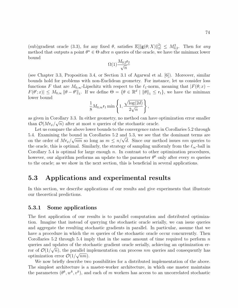


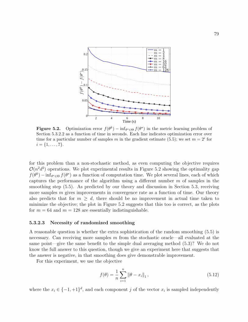


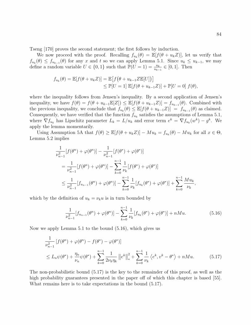

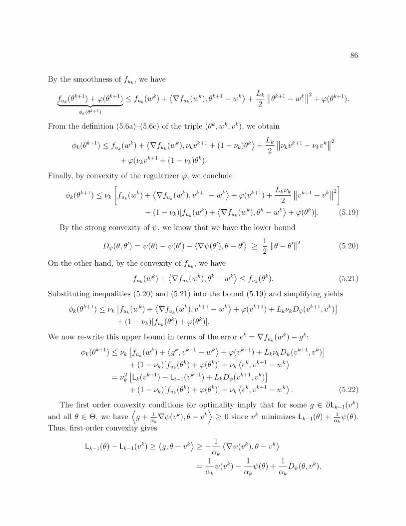


![Statistical guarantees for deep ReLU networks [1cm] · Imposing a statistical model Iassume (training) data are generated from a given statistical model Iimposed model can be simpler](https://static.documents.pub/doc/80x56/5f0e2ab87e708231d43dedfa/statistical-guarantees-for-deep-relu-networks-1cm-imposing-a-statistical-model.jpg)


