37
Multiple Path Pruning, Iterative Deepening and IDA* Alan Mackworth UBC CS 322 – Search 7 January 23, 2013 Textbook § 3.7.1-3.7.3
Multiple Path Pruning, Iterative Deepening and IDA*
Alan Mackworth
UBC CS 322 – Search 7
January 23, 2013
Textbook § 3.7.1-3.7.3
Lecture Overview
• Some clarifications & multiple path pruning
• Recap and more detail: Iterative Deepening and IDA*
2
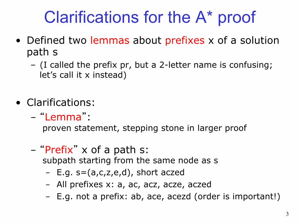
Clarifications for the A* proof • Defined two lemmas about prefixes x of a solution
path s – (I called the prefix pr, but a 2-letter name is confusing;
let’s call it x instead)
• Clarifications: - “Lemma”:
proven statement, stepping stone in larger proof
- “Prefix” x of a path s: subpath starting from the same node as s - E.g. s=(a,c,z,e,d), short aczed - All prefixes x: a, ac, acz, acze, aczed - E.g. not a prefix: ab, ace, acezd (order is important!)
3
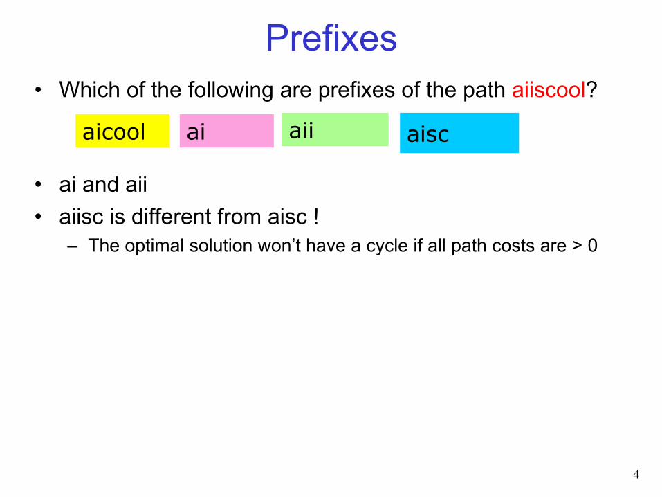
Prefixes • Which of the following are prefixes of the path aiiscool?
• ai and aii • aiisc is different from aisc !
– The optimal solution won’t have a cycle if all path costs are > 0
4
aisc aicool aii ai
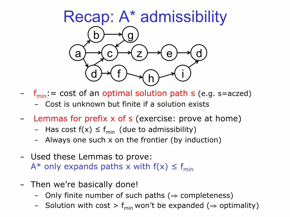
- fmin:= cost of an optimal solution path s (e.g. s=aczed) - Cost is unknown but finite if a solution exists
- Lemmas for prefix x of s (exercise: prove at home) - Has cost f(x) ≤ fmin (due to admissibility) - Always one such x on the frontier (by induction)
- Used these Lemmas to prove: A* only expands paths x with f(x) ≤ fmin
- Then we’re basically done! - Only finite number of such paths (⇒ completeness) - Solution with cost > fmin won’t be expanded (⇒ optimality)
Recap: A* admissibility
a c z e d
d f
b g
h i
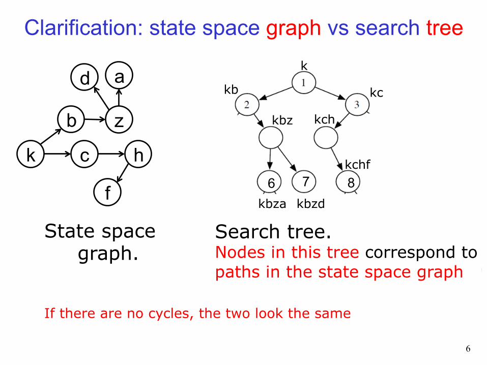
Clarification: state space graph vs search tree
6
k c
b z
h
akb kc
kbz
d
f kbza kbzd
kch
k
State space graph. If there are no cycles, the two look the same
Search tree. Nodes in this tree correspond to paths in the state space graph
kchfy
4 5
6 7 8
Clarification: state space graph vs search tree
7
k c
b z
h
akb kc
kbz
d
f kbza kbzd
kch
k
State space graph.
Search tree.
kchf
4 5
6 7 8
7
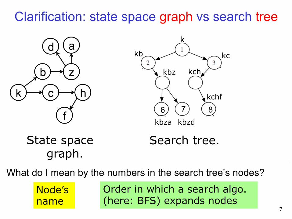
What do I mean by the numbers in the search tree’s nodes?
Node’s name
Order in which a search algo. (here: BFS) expands nodes
Clarification: state space graph vs search tree
8
k c
b z
h
akb kc
kbk kbz
d
f
kbkb kbkc
kbza kbzd
kch
kchf
kckb kckc
kck
k
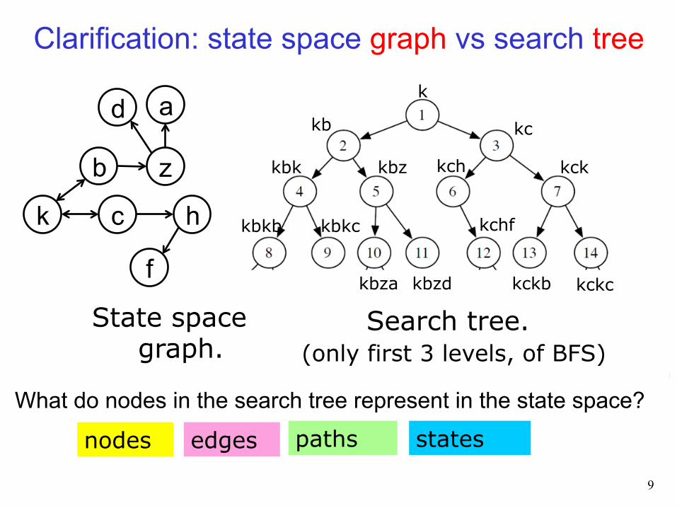
State space graph.
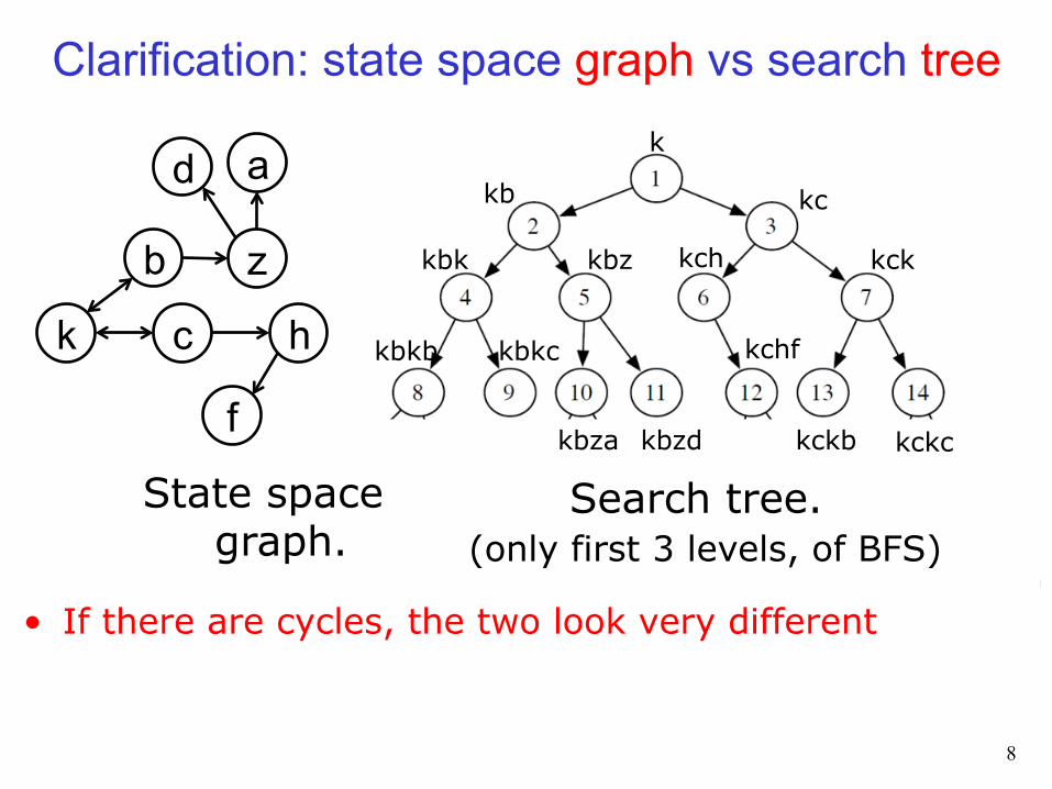
Search tree. (only first 3 levels, of BFS)
• If there are cycles, the two look very different
Clarification: state space graph vs search tree
9
k c
b z
h
akb kc
kbk kbz
d
f
kbkb kbkc
kbza kbzd
kch
kchf
kckb kckc
kck
k
State space graph.
Search tree. (only first 3 levels, of BFS)
What do nodes in the search tree represent in the state space?
states nodes paths edges

Clarification: state space graph vs search tree
10
k c
b z
h
akb kc
kbk kbz
d
f
kbkb kbkc
kbza kbzd
kch
kchf
kckb kckc
kck
k
State space graph.
Search tree. (only first 3 levels, of BFS)
What do edges in the search tree represent in the state space?
states nodes paths edges
Clarification: state space graph vs search tree
11
k c
b z
h
akb kc
kbk kbz
d
z
kbkb kbkc
kbza kbzd
kch
kchz
kckb kckc
kck
k
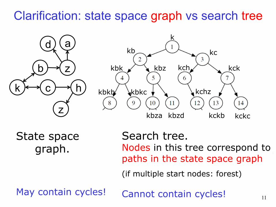
State space graph. May contain cycles!
Search tree. Nodes in this tree correspond to paths in the state space graph
(if multiple start nodes: forest)
Cannot contain cycles!
Clarification: state space graph vs search tree
12
k c
b z
h
akb kc
kbk kbz
d
z
kbkb kbkc
kbza kbzd
kch
kchz
kckb kckc
kck
k
State space graph.
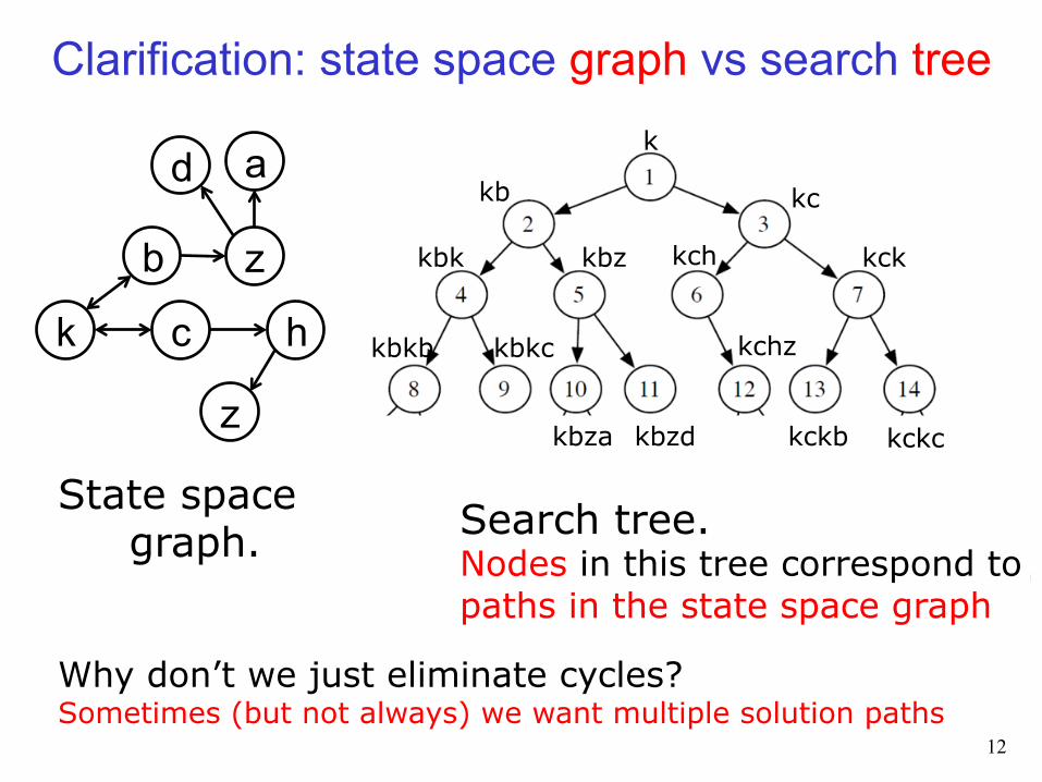
Why don’t we just eliminate cycles? Sometimes (but not always) we want multiple solution paths
Search tree. Nodes in this tree correspond to paths in the state space graph
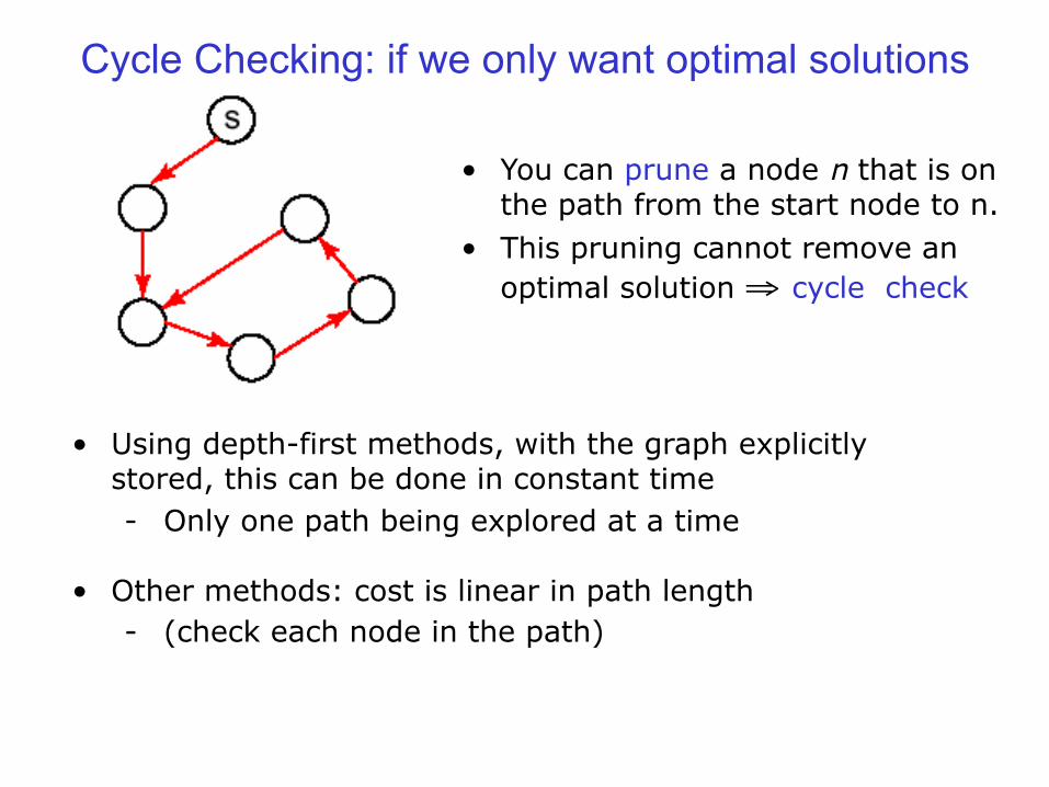
• Using depth-first methods, with the graph explicitly stored, this can be done in constant time - Only one path being explored at a time
• Other methods: cost is linear in path length
- (check each node in the path)
Cycle Checking: if we only want optimal solutions
• You can prune a node n that is on the path from the start node to n.
• This pruning cannot remove an optimal solution ⇒ cycle check
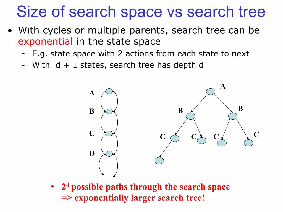
• With cycles or multiple parents, search tree can be exponential in the state space - E.g. state space with 2 actions from each state to next - With d + 1 states, search tree has depth d
Size of search space vs search tree
A
B
C
D
A
B B
C C C C
• 2d possible paths through the search space => exponentially larger search tree!
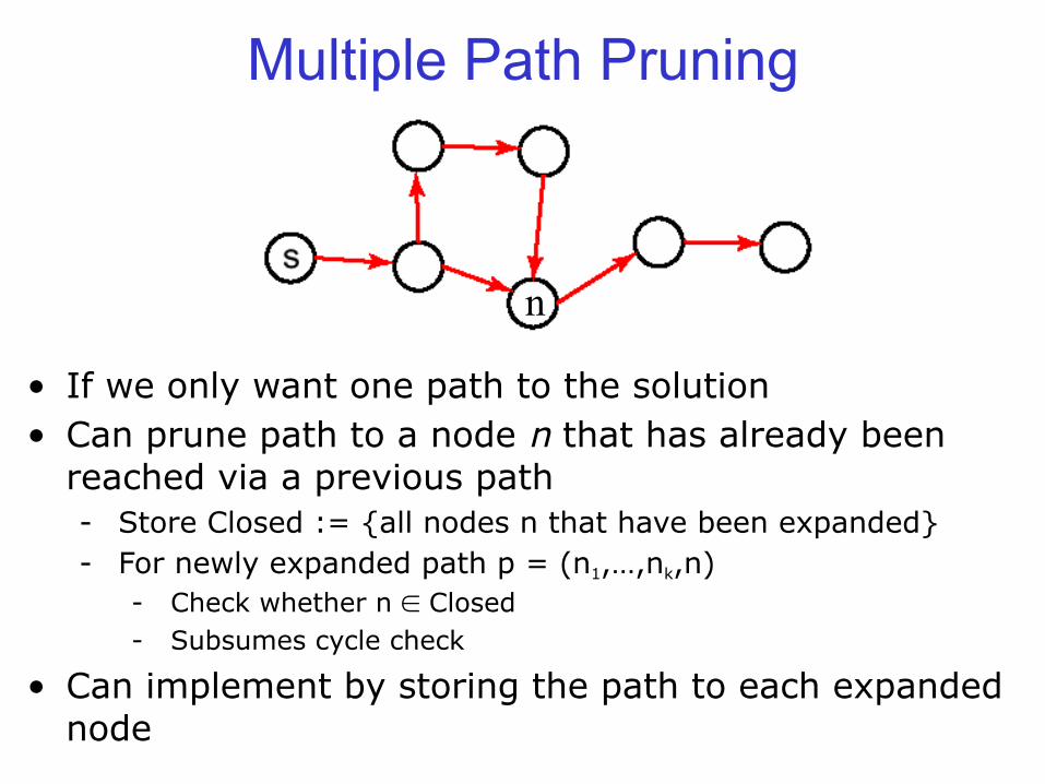
• If we only want one path to the solution • Can prune path to a node n that has already been
reached via a previous path - Store Closed := {all nodes n that have been expanded} - For newly expanded path p = (n1,…,nk,n)
- Check whether n ∈ Closed - Subsumes cycle check
• Can implement by storing the path to each expanded node
Multiple Path Pruning
n

Multiple-Path Pruning & Optimal Solutions
• Problem: what if a subsequent path to n is shorter than the first path to n, and we want an optimal solution ?
• Can remove all paths from the frontier that use the longer path: these can’t be optimal.
2 2
1 1 1
Multiple-Path Pruning & Optimal Solutions
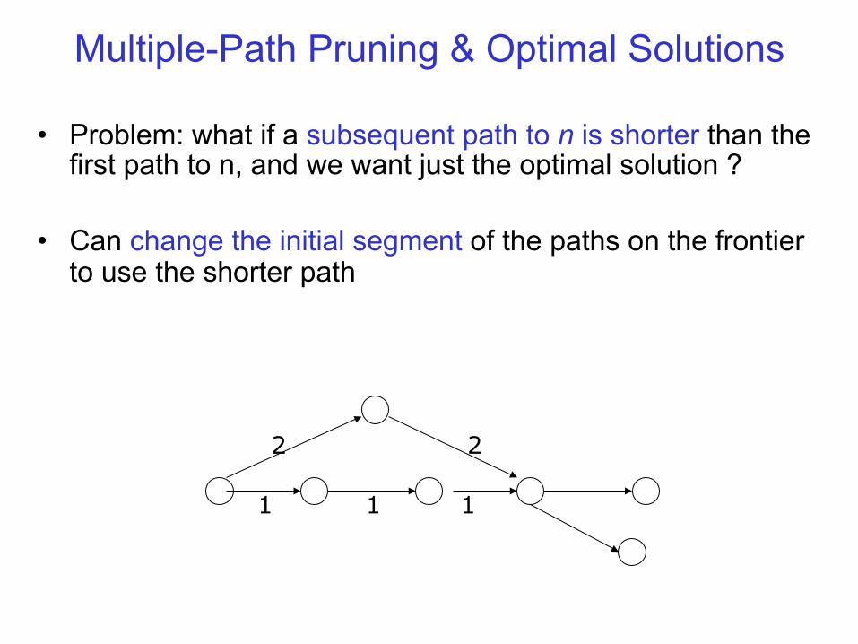
• Problem: what if a subsequent path to n is shorter than the first path to n, and we want just the optimal solution ?
• Can change the initial segment of the paths on the frontier to use the shorter path
2 2
1 1 1
Multiple-Path Pruning & Optimal Solutions
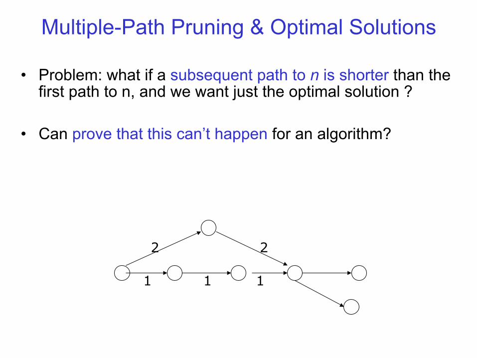
• Problem: what if a subsequent path to n is shorter than the first path to n, and we want just the optimal solution ?
• Can prove that this can’t happen for an algorithm?
2 2
1 1 1
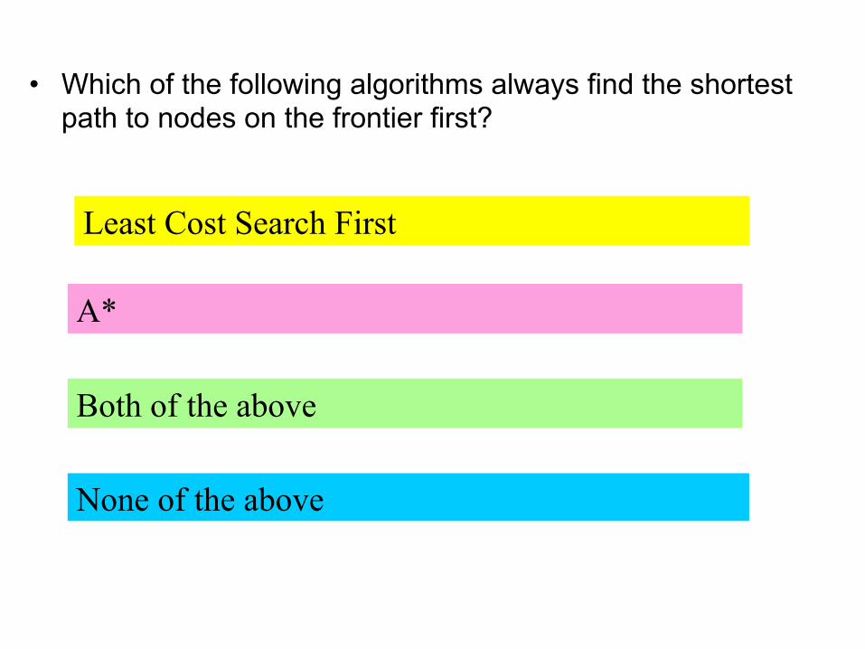
• Which of the following algorithms always find the shortest path to nodes on the frontier first?
None of the above
Least Cost Search First
Both of the above
A*
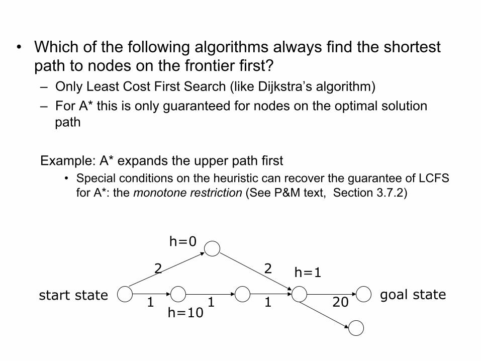
• Which of the following algorithms always find the shortest path to nodes on the frontier first? – Only Least Cost First Search (like Dijkstra’s algorithm) – For A* this is only guaranteed for nodes on the optimal solution
path
Example: A* expands the upper path first • Special conditions on the heuristic can recover the guarantee of LCFS
for A*: the monotone restriction (See P&M text, Section 3.7.2)
goal state h=10
h=0
h=1 2 2
1 1 1 20 start state
Summary: pruning • Sometimes we don’t want pruning
– Actually want multiple solutions (including non-optimal ones)
• Search tree can be exponentially larger than search space – So pruning is often important
• In DFS-type search algorithms – We can do cheap cycle checks: O(1)
• BFS-type search algorithms are memory-heavy already – We can store the path to each expanded node and do multiple path
pruning
21
Lecture Overview
• Some clarifications & multiple path pruning
• Recap and more detail: Iterative Deepening and IDA*
22
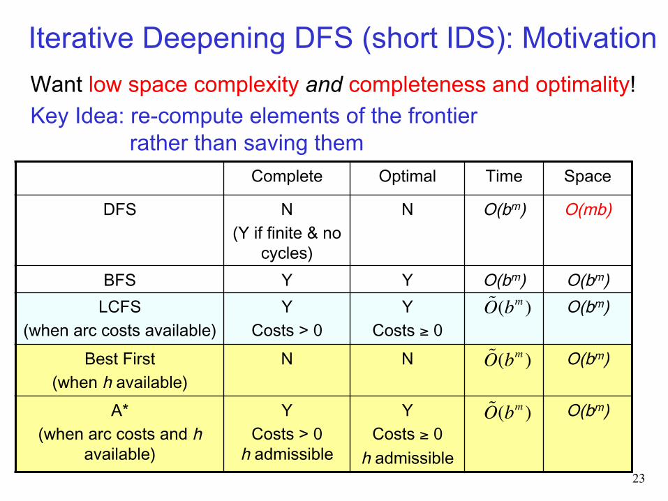
Want low space complexity and completeness and optimality! Key Idea: re-compute elements of the frontier
rather than saving them
23
Iterative Deepening DFS (short IDS): Motivation
Complete Optimal Time Space
DFS N (Y if finite & no
cycles)
N O(bm) O(mb)
BFS Y Y O(bm) O(bm) LCFS
(when arc costs available) Y
Costs > 0 Y
Costs ≥ 0 O(bm)
Best First
(when h available) N N O(bm)
A* (when arc costs and h
available)
Y Costs > 0h admissible
Y Costs ≥ 0 h admissible
O(bm)
O(bm )
O(bm )
O(bm )
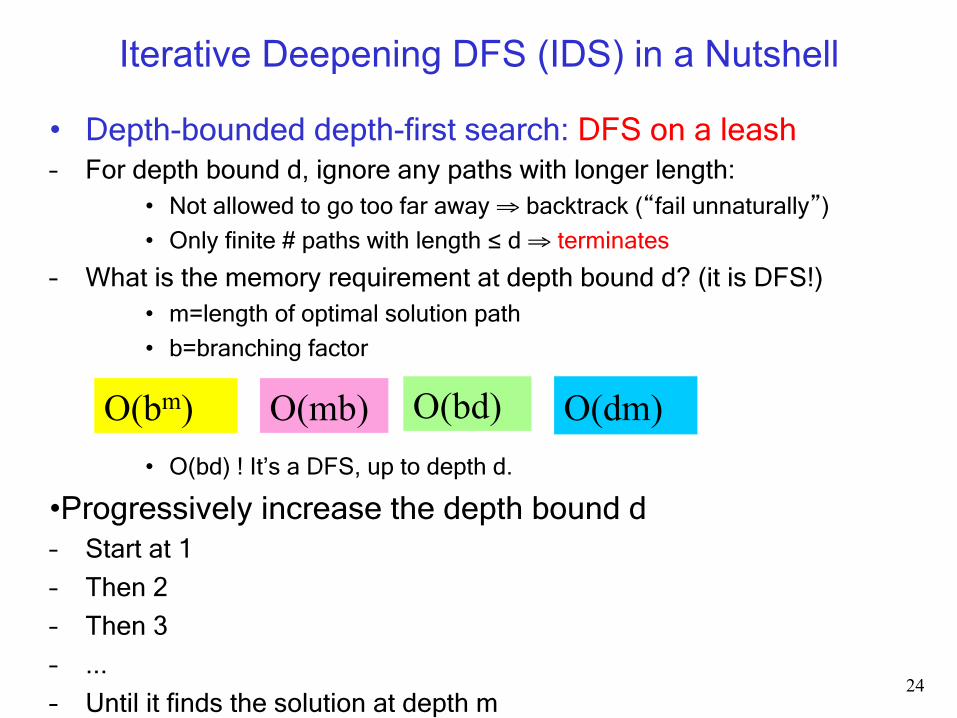
Iterative Deepening DFS (IDS) in a Nutshell
• Depth-bounded depth-first search: DFS on a leash – For depth bound d, ignore any paths with longer length:
• Not allowed to go too far away ⇒ backtrack (“fail unnaturally”)
• Only finite # paths with length ≤ d ⇒ terminates
– What is the memory requirement at depth bound d? (it is DFS!) • m=length of optimal solution path
• b=branching factor
• O(bd) ! It’s a DFS, up to depth d.
• Progressively increase the depth bound d – Start at 1
– Then 2
– Then 3
– ...
– Until it finds the solution at depth m 24
O(dm) O(bm) O(bd) O(mb)
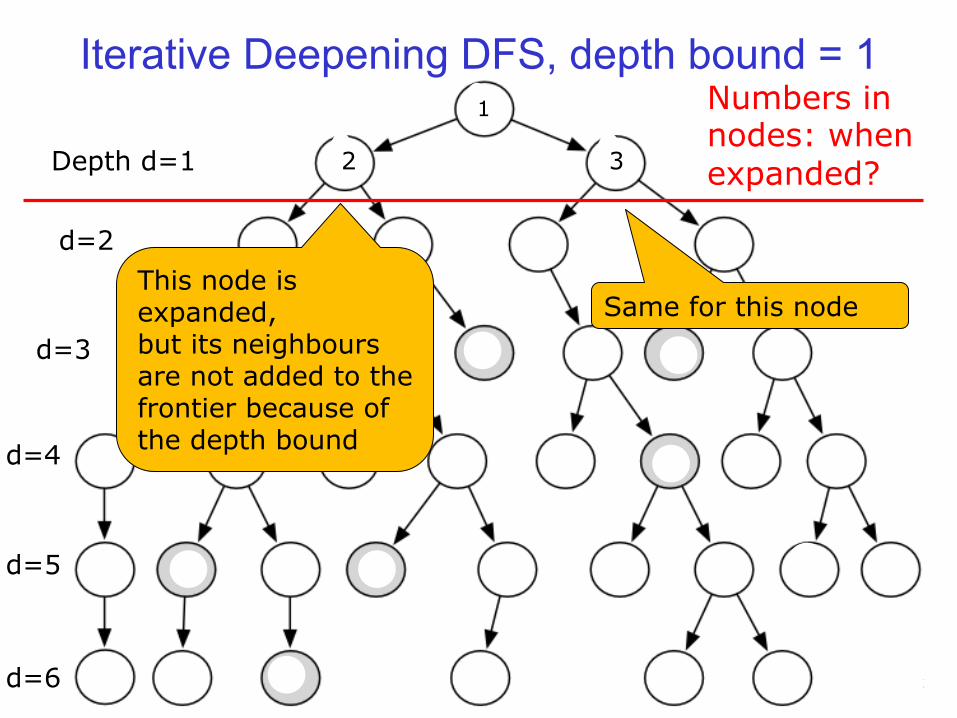
Iterative Deepening DFS, depth bound = 1
25
Example Depth d=1
d=2
d=3
d=4
d=5
d=6
3
This node is expanded, but its neighbours are not added to the frontier because of the depth bound
Same for this node
Numbers in nodes: when expanded? 2
1
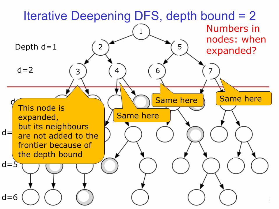
Iterative Deepening DFS, depth bound = 2
26
Example Depth d=1
d=2
d=3
d=4
d=5
d=6
2 5
3 4 6 7
Numbers in nodes: when expanded?
This node is expanded, but its neighbours are not added to the frontier because of the depth bound
Same here
Same here Same here
2
1
3 4
5
6 7
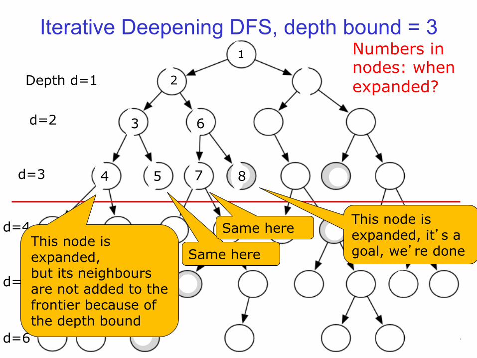
Iterative Deepening DFS, depth bound = 3
27
Example Depth d=1
d=2
d=3
d=4
d=5
d=6
2
Numbers in nodes: when expanded?
3
4 5
6
7 8
1
This node is expanded, but its neighbours are not added to the frontier because of the depth bound
Same here
Same here This node is expanded, it’s a goal, we’re done
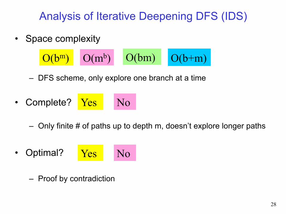
Analysis of Iterative Deepening DFS (IDS)
• Space complexity
– DFS scheme, only explore one branch at a time
• Complete?
– Only finite # of paths up to depth m, doesn’t explore longer paths
• Optimal?
– Proof by contradiction
28
O(b+m) O(bm) O(bm) O(mb)
Yes No
Yes No
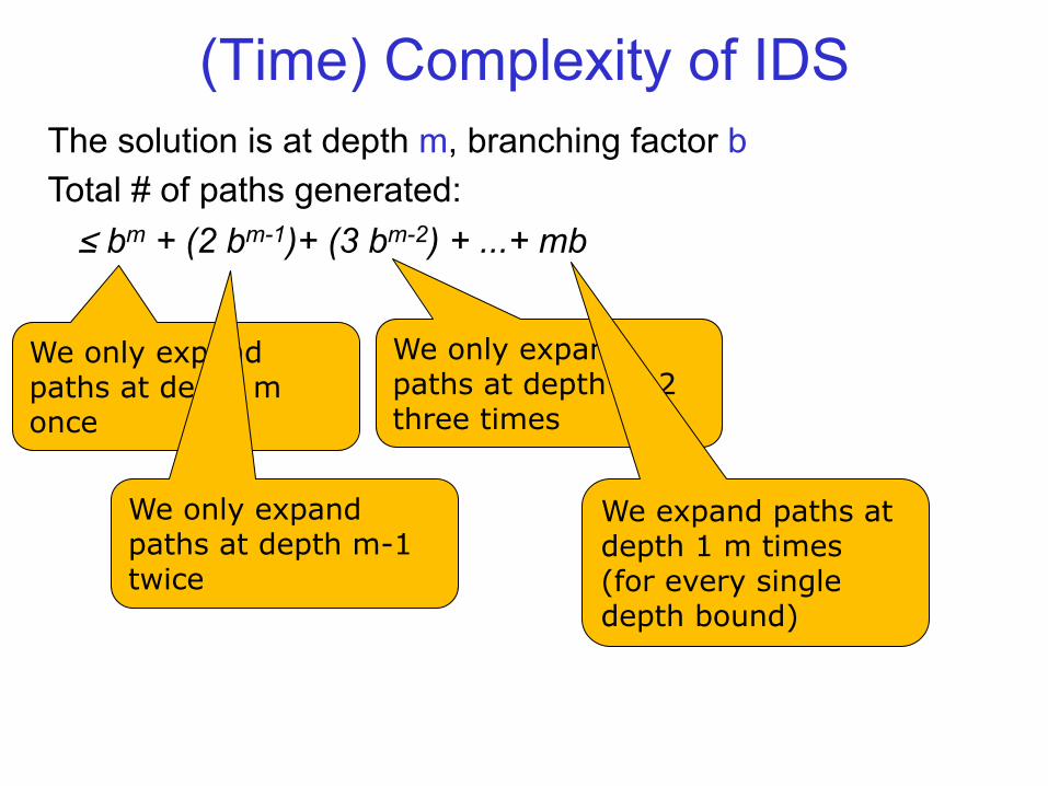
The solution is at depth m, branching factor b Total # of paths generated: ≤ bm + (2 bm-1)+ (3 bm-2) + ...+ mb
(Time) Complexity of IDS
We only expand paths at depth m once
We only expand paths at depth m-1 twice
We only expand paths at depth m-2 three times
We expand paths at depth 1 m times (for every single depth bound)

(Time) Complexity of IDS
)( mbO∈
))(()(1
11
1
1 ∑∑=
−−
=
− ==m
i
imm
i
im bibibb
rr
i
i
−=∑
∞
= 11
0 Geometric progression: for |r|<1:
20
1
0 )1(1r
irrdrd
i
i
i
i
−==∑∑
∞
=
−∞
=
))((0
11∑∞
=
−−≤i
im bib2
111
⎟⎠
⎞⎜⎝
⎛−
=−b
bm2
1⎟⎠
⎞⎜⎝
⎛−
=bbbm
If b > 1
From there on, it’s just math: Total # paths generated by IDS ≤ bm + (2 bm-1)+ (3 bm-2) + ...+ mb = bm (1 b0 + 2 b-1 + 3 b-2 + ...+ m b1-m )
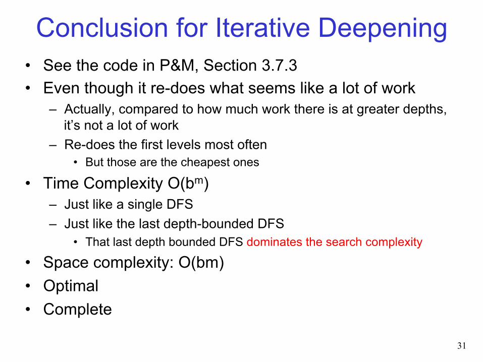
Conclusion for Iterative Deepening • See the code in P&M, Section 3.7.3 • Even though it re-does what seems like a lot of work
– Actually, compared to how much work there is at greater depths, it’s not a lot of work
– Re-does the first levels most often • But those are the cheapest ones
• Time Complexity O(bm) – Just like a single DFS – Just like the last depth-bounded DFS
• That last depth bounded DFS dominates the search complexity
• Space complexity: O(bm) • Optimal • Complete
31
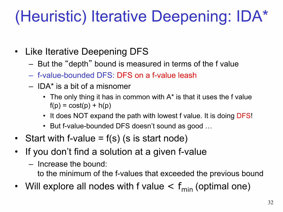
(Heuristic) Iterative Deepening: IDA* • Like Iterative Deepening DFS
– But the “depth” bound is measured in terms of the f value – f-value-bounded DFS: DFS on a f-value leash – IDA* is a bit of a misnomer
• The only thing it has in common with A* is that it uses the f value f(p) = cost(p) + h(p)
• It does NOT expand the path with lowest f value. It is doing DFS! • But f-value-bounded DFS doesn’t sound as good …
• Start with f-value = f(s) (s is start node) • If you don’t find a solution at a given f-value
– Increase the bound: to the minimum of the f-values that exceeded the previous bound
• Will explore all nodes with f value < fmin (optimal one) 32
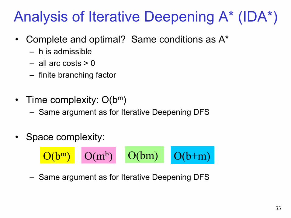
Analysis of Iterative Deepening A* (IDA*) • Complete and optimal? Same conditions as A*
– h is admissible – all arc costs > 0 – finite branching factor
• Time complexity: O(bm) – Same argument as for Iterative Deepening DFS
• Space complexity:
– Same argument as for Iterative Deepening DFS
33
O(b+m) O(bm) O(bm) O(mb)
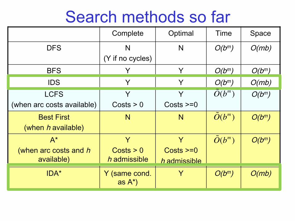
Search methods so far Complete Optimal Time Space
DFS N (Y if no cycles)
N O(bm) O(mb)
BFS Y Y O(bm) O(bm) IDS Y Y O(bm) O(mb)
LCFS (when arc costs available)
Y Costs > 0
Y Costs >=0
O(bm)
Best First (when h available)
N N O(bm)
A* (when arc costs and h
available)
Y Costs > 0h admissible
Y Costs >=0 h admissible
O(bm)
IDA* Y (same cond. as A*)
Y O(bm)
O(mb)
O(bm )
O(bm )
O(bm )
• Define/read/write/trace/debug different search algorithms - In more detail today: Iterative Deepening,
Iterative Deepening A*
• Apply basic properties of search algorithms: – completeness, optimality, time and space complexity
Announcements:
– Practice exercises are out on home page. • Heuristic search • Please use them! (Only takes 5 min. if you understood things…)
– Assignment 1 is out: see Connect
35
Learning Goals for today’s class
Learning Goals for search • Identify real world examples that make use of deterministic,
goal-driven search agents • Assess the size of the search space of a given search
problem. • Implement the generic solution to a search problem. • Apply basic properties of search algorithms:
- completeness, optimality, time and space complexity • Select the most appropriate search algorithms for specific
problems. • Define/read/write/trace/debug different search algorithms • Construct heuristic functions for specific search problems • Formally prove A* optimality. • Define optimally efficient

Coming up: Constraint Satisfaction Problems
• Read chapter 4
• Get busy with assignment 1
37


