Engineering Costs and Production Economics, 16 ( 1989) 245-256 Elsevier Science Publishers B.V., Amsterdam -Printed in The Netherlands 245 MULTIPLE PRODUCT INVENTORY POLICIES WITH UNIT LOAD AND STORAGE SPACE CONSIDERATIONS Susan Schall and Jeya Chandra Department of Industrial and Management Systems Engineering, The Pennsylvania State University, University Park, PA 16802 (U.S.A.) ABSTRACT In this paper the appropriate unit load for Load (EUL) method is revised to include mul- each product in a multi-product inventory sys- tiple container types and the Equal Order Inter- tern is determined and used to calculate the best val (EOI) method is extended to consider unit policy given limited storage space. An inventory loads andjinite replenishment rates. The meth- system with constant demand and replenish- ods are compared using total cost and average ments rates is considered. The Economic Unit space utilization as the criteria. INTRODUCTION Within the total production system there are thousands of manufacturers producing goods for millions of customers. The major difficulty in this system is that customers do not demand the products at the same rate that producers produce them. Customers want the product only when they need it; producers want to maintain a uniform production rate. As a re- sult of this difference, the customer and/or producer must maintain a supply of the prod- uct. This raises the question: How much in- ventory should be kept on hand and what are the storage requirements? A production manager faced with the above question must minimize the order cost while minimizing the amount of space required. Space used for storage costs money and pre- vents the space from being used for a more productive purpose. Often the amount of space available is restricted by the physical layout of the plant. As a result, the production manager would like to utilize the space as much as pos- sible. The problem is further complicated by the fact that few manufacturing and storage fa- cilities deal with a single type of part. The parts are often of many different shapes, sizes, and weights. The parts may also be stored and transported in a variety of containers. Ideally, one would like to have all of the parts, regard- less of their characteristics, stored in the same size and type of container. This makes trans- portation and storage much easier. Due to weight and volume constraints, however, a container that is good for one part may not be appropriate for another part. The type of stor- age space needed then will depend on the type and size of the containers chosen and the max- imum expected inventory of each item. Most inventory models developed to date fail to take into account the physical characteris- tics of the parts and their containers, and the space available. Tanchoco et al. [ 1 ] included the concept of the unit load into Wilson’s sin- gle product EOQ model and named it the Eco- 0167-188X/89/$03.50 0 1989 Elsevier Science Publishers B.V.
Transcript
Engineering Costs and Production Economics, 16 ( 1989) 245-256 Elsevier Science Publishers B.V., Amsterdam -Printed in The Netherlands
245
MULTIPLE PRODUCT INVENTORY POLICIES WITH UNIT LOAD AND STORAGE SPACE CONSIDERATIONS
Susan Schall and Jeya Chandra Department of Industrial and Management Systems Engineering, The Pennsylvania State University, University Park, PA
16802 (U.S.A.)
ABSTRACT
In this paper the appropriate unit load for Load (EUL) method is revised to include mul- each product in a multi-product inventory sys- tiple container types and the Equal Order Inter- tern is determined and used to calculate the best val (EOI) method is extended to consider unit policy given limited storage space. An inventory loads andjinite replenishment rates. The meth- system with constant demand and replenish- ods are compared using total cost and average ments rates is considered. The Economic Unit space utilization as the criteria.
INTRODUCTION
Within the total production system there are thousands of manufacturers producing goods for millions of customers. The major difficulty in this system is that customers do not demand the products at the same rate that producers produce them. Customers want the product only when they need it; producers want to maintain a uniform production rate. As a re- sult of this difference, the customer and/or producer must maintain a supply of the prod- uct. This raises the question: How much in- ventory should be kept on hand and what are the storage requirements?
A production manager faced with the above question must minimize the order cost while minimizing the amount of space required. Space used for storage costs money and pre- vents the space from being used for a more productive purpose. Often the amount of space available is restricted by the physical layout of the plant. As a result, the production manager
would like to utilize the space as much as pos- sible. The problem is further complicated by the fact that few manufacturing and storage fa- cilities deal with a single type of part. The parts are often of many different shapes, sizes, and weights. The parts may also be stored and transported in a variety of containers. Ideally, one would like to have all of the parts, regard- less of their characteristics, stored in the same size and type of container. This makes trans- portation and storage much easier. Due to weight and volume constraints, however, a container that is good for one part may not be appropriate for another part. The type of stor- age space needed then will depend on the type and size of the containers chosen and the max- imum expected inventory of each item.
Most inventory models developed to date fail to take into account the physical characteris- tics of the parts and their containers, and the space available. Tanchoco et al. [ 1 ] included the concept of the unit load into Wilson’s sin- gle product EOQ model and named it the Eco-
nomic Unit Load (EUL) model. In a later ar- ticle, Tanchoco, et al. [ 21 expanded the model to a multi-product inventory system. They, however, assumed that all of the products could and would be stored in only one size/type of container and did not attempt to maximize the utilization of the available storage space. Page and Paul [ 3 ] attempted to maximize the space utilization by adjusting the order intervals of the products. They, however, did not include the concept of the unit load in their model (known as the Equal Order Inventory or EOI model ) .
In this paper, a method of determining the appropriate container type for each product in a multi-product inventory system will be given. First, the EUL model with just one type con- tainer developed by Tanchoco et al. [ 3 ] will be modified to include multiple types of con- tainers. Then, the EOI model developed by page and Paul [ 31 with infinite replenishment rate and no consideration for unit load will be extended to situations with finite replenish- ment rates and unit loads. An example will be given and the results in term of total cost and space utilization compared.
ASSUMPTIONS AND NOTATION
The model developed in this paper makes the following assumptions: 1. Shortage is not allowed. 2. A given product is stored in only one type of
container. 3. Block stacking (storage of unit loads in
stacks within storage rows [ 41 is used to store the products. Block stacking is used when a large quantity of a few products are stored and stacking is permissible. It is used primarily for food, beverage, appliance and paper storage to achieve high space utiliza- tion at a low cost.
4. A stack contains only one product. 5 Products are not replenished at a constant
rate. 6. Containers are transported one at a time.
7. Demand rate is constant and continuous. The following notation will be used through-
out this paper:
m n
Cl/
c3j
cmj
5 Pi
Imax,
Aj A
1 I’ [ l-
Number of products Number of different containers Carrying cost for product j per unit
time, [$l/[Tl Replenishment cost for product j per
order, [$l/[Tl Material handling cost per move for product j, [ $ ] / [move]
Demand for product j per unit time Production for product j per unit time,
Pj> rj Order quantity of product j Number of units of product j in se- lected container, unit load Maximum inventory or productj Area required by product j at Imax, Available area Value rounded up to nearest integer Truncation to integer value
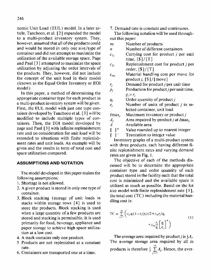
Inventory graphs of a multi-product system with three products, each having different ti- nite replenishment rates and varying demand rates are given in Fig. 1.
The objective of each of the methods dis- cussed will be to determine the appropriate container type and order quantity of each product stored in the facility such that the total cost is minimized and the available space is utilized as much as possible. Based on the lot size model with finite replenishment rate [ 5 1,
the total cost (TC) including the material han- dling cost is:
TC = ? c,,q,( 1 -r,lp,)12+c~lr,lq, ,=I (1)
The average area required by productj is fAj.
The average storage area required by all m
products is therefore f f AI. Hence, the aver- /=1
247
Product 1
Product 3
time
Fig. 1. Inventory graphs of multi-product system with finite replenishment rates and varying demand rates.
age space utilization in terms of floor space may be calculated as:
Utilization= 4 f AJA ,=1
(2)
DETERMINATION OF UNIT LOAD
The first item that must be determined for each product is the size of the unit load. In his book, Materials Handling System Design, Ap- ple [ 61 defines a unit load as “a single item, a number of items, or bulk material so arranged or restrained that the mass can be picked up and moved between two locations as a single object”. A unit load may take the form of a container, bin, pallet, or any other carrying unit. The size/type of container determines the number of items that can be moved and stored as a single unit.
The container chosen will depend on the weight and volume characteristics of the prod- uct along with the dimensions of the product.
The volume constraint can be expressed in terms of the number of items that can fit into a given container:
where: e; maximum number of product j in con-
tainer i due to the volume constraint k$ fill ratio or packing factor of productj in
container i; the ratio between the total volume occupied by product j and the total volume of container i; 0 c k; d 1 .O
*i width of container i 1, length of container i hi height of container i
vj unit volume of product j Similarly, the weight constraint can be ex-
pressed in terms of the weight of the product and the capacity of the material handling device:
(4)
248
where:
et maximum number of product j in con- tainer i due to the weight constraint
K” rated weight capacity of material han- dling method
IV dead weight of container i
WJ unit weight of product j It can be seen from the above equations that
the analyst must have a list of possible con- tainer sizes that can be used. This information can be obtained by surveying the present stor- age facility and by contacting storage con- tainer suppliers. Once the formation is ob- tained, it can be used to calculate e; and e; for each combination of i and j. To choose the proper container for product j, let elj= min{e’;, el;} since to choose otherwise would violate one or both constraints. Then let
e,= [max,,, i{ej,}] for all j= 1, 2, . . . . m
This allows both the volume and weight con- straints to be satisfied while at the same time minimizes the number of containers and hence the number of moves required to transport a given amount of product j. Once e,, j= 1, 2, . . . . m, is determined, the number of units per unit load is fixed. If all but one container drops out of consideration, the problems reduces to the EUL model described by Tanchoco et al. [ 1 ]
and can be solved as such (see Appendix A). Otherwise, the combination of the container sizes will affect the final solution. In the next section, the basic EUL model with just one type of container will be modified to consider mul- tiple types of containers.
MODIFIED EUL SOLUTION METHODOLOGY
The first step in the EUL model after the de- termination of the container sizes is the calcu- lation of the initial order quantity for each of the products and the maximum space required to store them. The initial order quantity is sim-
ply the optimal EOQ for the unit loads:
J %c, 1 qy= ~ cl, Cl-q/p,)
q,=e,Iq,“le,l+ (6)
Imax, = [ 4, ( 1 - r,lp, 1 I + (7)
The space required must then be compared
order quantity adjusted
(5)
to the available space. The storage constraint may be expressed in terms of the number of stacks of each container type that will lit within the available space:
,c, +‘,c, 6 GA (8)
where: n $ = number of stacks of product j in container i, lizlength of container i, wi=width of container i,
(9)
where: kh = available stacking height, and h,= height of the container selected to store product j.
Due to the shape of the containers it is pos- sible that constraint (8) is met but that the shape of the available storage space may not accommodate the required number of stacks. For our purposes this will be assumed negligible.
The problem may be unconstrained - there may be enough storage space available to store all the products. In that case the analyst has found a solution that will minimize the total cost. The space may not be fully utilized, how- ever. In most cases, though, this will not hap- pen. The method given here will assume that the problem is constrained.
When the storage constraint is not satisfied, the order quantity of one or more products must be reduced by at least one stack. The product(s) chosen must minimize the in- crease in the total cost of the system. The pro- cess is iterative in nature, reducing the system by one stack at a time until the storage con-
straint is satisfied. Unlike the EUL method, the number of iterations needed to satisfy the stor- age constraint is dependent on the sizes of the containers.
Solve the problem as follows: 1.
2.
3.
4.
5.
6.
Compare the results of the initial calcula- tions to the storage constraint. If the storage constraint is met + GOT0 5. Calculate the change in total cost for each product for a reduction in q by one stack. Choose product j which has the minimum increase in cost. Reduce the number of stacks appropriately and recalculate Imax, and q,, where:
Imax,=n;e, (10)
q,=Imax,l(l-5/p,) (11)
Calculate the storage requirement with the new order quantity and compare to the stor- age constraint. Repeat steps 2 and 3 until the storage con- straint is met. Calculate the storage requirement for each product and container type and the average space utilization. STOP An example problem is included later to il-
lustrate the use of this procedure.
EOI METHODOLOGY
The maximum space utilization possible by the EUL method is 50%. The reasoning for this is that at certain points in time all m products will simultaneously reach their maximum in- ventory which must not require more than the maximum available floor space. The EOI model developed by Page and Paul [ 3 ] is an alternative to the EUL method in which the m products are not permitted to reach their max- imum inventories at the same time. This is achieved by staggering the replenishments of the products and assigning the same cycle time to each of the products (see Appendix B). Their model, which considered infinite replen-
249
ishment rates without unit loads, will be ex- panded in this section to include finite replen- ishment rates and unit loads. As will be shown shortly, the introduction of finite replenish- ment rates and unit load constraints will intro- duce considerable computational difficulties. Thus a heuristic procedure will be used to de- termine a policy which results in a better utili- zation of space than the EUL model while minimizing the total cost of the system. The method of determining the appropriate unit load as described earlier will be used.
The inventory graphs of a three-product sys- tem with staggered replenishments and equal cycle times (t) for each product are given in Fig. 2. Let us also assume that the products are numbered in the same sequence in which they are replenished. The time interval between the start of replenishment of productj and the start of the replenishment of product (j+ 1) will be denotedbyt,+,,j=1,2 ,..., m-l andthetime interval between the start of replenishment of product m and product 1 will be denoted by t,. It can be seen from Fig. 2 that:
,$, t,=t (12)
The inventory policy now reduces to that of finding the values oft,, j= 1,2, . . . . m (and hence t ) such that the available space is utilized each time a product reaches its maximum inven- tory level.
As there are m unknown independent deci- sion variables (tj, j= 1, 2, . . . . m), m equations are needed. These equations can be formu- lated by relating the total space required each time a product reaches its maximum inven- tory to the total available space. Let Invj,k be the inventory level of the product k when productj reaches its maximum inventory level and let Aj,k be the area required to store the quantity Invj,k in the warehouse. The relation- ship between Invj,k and A,,k is:
r[&hl +i+
A,.k = l,w,, j&=1,2 ,..., m (13)
250
Product 1
time
time
Fig. 2. Inventory graphs with staggered replenishment and equal cycle times.
The m equations needed to find the values oft,& 1, 2, . ..) m can now be written as:
? A,,, <A, k=l
j= 1, 2, . . . . m (14)
or
l,w,<A, j=l,2, . . . . m (15)
Invj,k, however, must be written as functions of the unknown variables tj, j = 1, 2, . . . . m be- fore the system of equations can be solved.
From the finite replenishment rate EOQ model [ 5 1, the maximum inventory of prod- uctj, Inv,,, can be expressed as:
lnv,,,=q,(l-r,lp,), j=l, 2, . . . . m (16)
where:
4/ = 5 t (Ii
and t is the common cycle time (replenish- ment period) that is equal to the sum of the tj, j=l,2 m. , -0.3
The inventory levels of products 2 and 3 at the point in time when product 1 reaches its maximum inventory level can be found using the vertical line AA in Figure 2. Using eqn. (16), Inv,,l is simply:
tnvl,,=q,(l--r,lp,) (18)
Inv, ,2 is the height CD (in Fig. 2 ) which de- pends on the slope of line XY and the time in- terval XD. As line XY is the replenishment line, its slope is (pz- y2). As tz, which is the time interval between the starting of the replenish-
251
ments of products 1 and 2, is less than q,/p, in the figure, the time interval XD is ( q1 /p, - t2). Hence CD is (ql/pl-tZ)x (p2-rz). On the other hand, if t2 > q1 /p,, then the line AA inter- sects the demand line YZ, the slope of which is r2. the inventory level of product 2 at the time of interest is therefore ( t2-ql/pl ) x r2. Com- bining these two results, Inv1,2 may be written as:
(t,+,+t,+z+...t,+t,+...+tk), j>k forj=l,2 ,..., m-l andk=l,2 ,..., m
(23)
and
Sum,,k=t, +tZ+...+tk, forj=m,
k= 1, 2, . . . . (m- 1) (24)
Using eqns. (22), (23), and (24), the m equations in ( 15 ) may now be written in terms oft,,j=l,2, . ..) m. It should be noted that the values Of tj,j= 1, 1, . . . . m in eqns. (22), (23), and (24) are unknown as is the value of qj This introduces a problem in the solution of eqn. ( 15 ), primarily due to the presence of terms with [ ] +. Optimal closed form solutions can
not be developed. Instead, a heuristic proce- dure developed by the authors will be suggested.
Heuristic
Upon examination of eqns. (22), (23)) and (24)) it can be seen that there is one term with only one t, in each equation. More specifically, for equation j, IIlVjj+ 1 contains only tj+, for j= 1, 2, . ..) m - 1 and for equation m, Inv,, ,
contains only tl. The heuristic procedure will utilize this property of the equations and use it to iteratively determine the values of tQ, 1= 1, 2 , a**> m until successive values of tp differ by some prespecilied E, or until the total cost per unit time and the space utilization reach some desired values.
Starting values oft and tp, I= 1, 2, . . . . m are needed to begin the procedure. One candidate for the starting value oft is the optimum value of the common cycle time as obtained without consideration of the constraints imposed by the unit loads or space availability. The optimum value is obtained by differentiating the total cost equation given in eqn. (25) and setting the derivative equal to zero.
TC= f (c,,q,(t -r,lp,)/2+c,,lt) (25) ,=I
The optimum cycle time t* is given in eqn. (26)
? c3, +J, J=’
C %(l -r,lp,) (26)
,=I 2
Candidates for the starting values of tp are simply tp =t*/m, II= 1, 2, . . . . m.
Arrange and number the products in de- creasing order of the ratio of the demand rate to the replenishment rate, rj/pj, j= 1, 2, . . . . m. The heuristic can now be described in terms of the following steps: 1. Set t equal to the optimum common cycle
time as determined by eqn. (26).
252
2. Set tl=t2=...=tm=t*/m. 3. Set j= 1 and g= 2. 4. Using term j of eqn. ( 15) and the current
valuesoftandtp,II=1,2,...,m,findthesum
1 A,k kig a. If C A,,k<A -+ GOT0 5.
k+g b. If x Aj,k> A + GOT0 6.
kf-g c. If x A,,+4 -+ GOT0 7,
k#S 5. Determine the differences / C Aj,k-A I.
k#g
Find the value of tg using the difference and Ar,k. -+ GOT0 8. Set t=t- At, where At is a small prespeci- fied value. a. If t> 0 - GOT0 2. b. It t-=z ~0, the system may not have a fea-
the average space utilization, and the maximum space utilized when each prod- uct reaches its maximum level of inven- tory. If satisfactory, GOT0 9. Otherwise, GOT0 3.
b. Ifj<m, then setj=j+ f. and g=g+ 1 (or g= I if g+ 1 > m), GOT0 4.
9. STOP. An example will be given in the next section
to illustrate the use of this heuristic.
EXAMPLE PROBLEM
The example problem discussed in this sec- tion is a modification of the example included in the EUL article by Tanchoco et al. [ 11.
The problem consists of five products and three containers. The product characteristics are shown in Table 1 and the characteristics of the available containers are shown in Table 2. The inventory costs and storage constraints are as follows: A = 4000 in.2
Area required=3924 in.2, total cost=$22,072.93, average utilization =49.05%.
Kh= 36 in. KW= 550 lb K; =0.70 for all isj cg= $0.1 S/unit/yr, for all j
csj= $20/s& up, for allj Cmj= $4.6O/move, for all j
A computer program was written in BASIC on the IBM-PC to perform the EUL calcula- tions and a summary report was obtained. Ta- bles C-l-C-4 in Appendix C show the inter- mediate results for e;, e$, eg and e,. The initial
EOI Set I $22,205.66 3744 64.32% 15% increase in utilization
EOI Set II $22,178.81 4068 74.25% space exceeded EOI Set III $22,166.70 4176 76.05% space exceeded
and final values and the resulting costs are listed in Table 3. Sample iteration results are also given in Tables C-5 and C-6 in Appendix C.
The procedure was repeated using Tancho- co’s original EUL model with just one con- tainer type. The results of the calculations are shown in Table 4. Given these results, con- tainer 3 would have been chosen at a cost of
$22,703.28, an increase of $630.35 from the modified multiple container method, and a decrease in space utilization of 0.45%. The use of two containers, therefore, can result in de- creased costs and increased space utilization. If material handling costs vary by container type or are increased due to the need to handle multiple container types, this may not be true. These costs should be taken into consideration when making the final decision.
A computer program written in BASIC on the IBM-PC was used to perform the calcula- tions of the EOI heuristic. Some resulting so- lution sets are given in Table 5. Intermediate calculations are given in Table C-7 in Appen- dix C. In the first solution set, the total space utilized by all products when each product reaches its maximum inventory level is less than the available space. The average space utilized is 64.32% and the total cost is $22,205.66 per year. In comparison to the pre- vious EUL model, this is a 15.3% increase in space utilization and less than a 1% increase in cost. In the other two solution sets, the storage space required when a product reaches maxi- mum inventory is slightly greater than the space available. As the amount of excess space required is less than 5% of the available space, it may be possible to use some addition space near by or to temporarily allow stacks to con- tain more than one type of product, thus re- sulting in an overall improvement in space uti- lization and a decrease in total cost. The results are compared in Table 6.
CONCLUSIONS
A storage facility may contain products of many different shapes, sizes, and weights. These differences may dictate the use of sev- eral container types. A method of determining the best container for a particular product given volume and weight constraints was presented in this paper. The container size determined the unit load size and was used together with the demand and production rates to determine
254
the initial order quantities and storage require- ments. Two previous methods, the EUL method developed by Tanchoco et al. [ 1,2] and the EOI method developed by Page and Paul [ 3 ] were then modified to determine the appropriate order quantities using multiple containers within the same storage space. The EUL method originally proposed by Tanchoco et al. considered block stacking but did not al- low the selection of more than one container type. The Page and Paul EOI model did not include containers at all and assumed an infi- nite replenishment rate. An example was given to demonstrate the two modified methods. In the example used, the EUL model with multi- ple container types was found to be slightly better than the EUL model with only one con- tainer type, but did not maximize the space utilization. As mentioned earlier, the addi- tional costs due to use of multiple types of con- tainers should be taken into consideration be- fore making the final decision. The EOI model using a heuristic developed by the authors had slightly greater costs compared to the EUL model but much improved space utilization. As the EOI model staggers replenishment, the uti- lization should be greater than the EUL model. Therefore, the EOI model can be used to deter- mine the order quantities and cycle times needed to stagger replenishment in order to improve space utilization, when feasible. In real life applications, the user should find the optimal inventory policy after taking all the relevant costs into account.
Many companies in the 1980s are imple- menting and/or using Just-in-Time (JIT) in- ventory policies to reduce their inventories and
hence the amount of warehouse or in-process space no longer becomes a constraint. But, the
implementation of JIT and its effect do not oc- cur overnight; it is usually a process of evolu-
tion requiring Total Quality Control and em- ployee training in addition to process modification. The modified EUL and EOI
methods presented in this paper can still be used during implementation of JIT. The re-
sults can serve as guidelines for the intermedi-
ate storage space reduction goals desired by the company.
REFERENCES
Tanchoco, J.M., Davis, R.P. and Wysk, R.A., 1980. Eco- nomic order quantities based on unit load and material handling considerations. Decision Sci., 11 (3 ), 5 14-52 1.
Tanchoco, J.M., Davis, R.P., Egbelu, P.J. and Wysk, R.A., 1983. Economic unit loads for multi-product inventory- systems with limited storage space. Mat. Flow, 1: 14 l- 148.
Page, E. and Paul, R.J., 1987. Multi-product inventory situ- ations with one restriction. Oper. Res. Q., 27 (4): 8 16- 833.
Tompkins, J.A. and White, A., 1984. Facilities Planning. John Wiley & Sons, New York.
Naddor, E., 1966. Inventory Systems. Robert E. Krieger Pub- lishing Company, Malabar, FL.
Apple, J.M., 1972. Material Handling System Design. Ron- ald Press, New York.
(Accepted December 8, 1987)
APPENDIX A
EUL solution methodology
The EUL solution method developed by Tanchoco et al. [ 2 ] for a multi-product inven- tory system is a follows: 1. Calculate the optimum order quantity (qj)
for each product, j= 1, . . . . m, without con- sideration of the storage space constraint.
4,=J(2r,c~,,lc,,)(ll(l-r,/p,)) (A-1 1
2. Determine the number of unit loads re- quired for each product using container i: +
(A-2)
where ej is determined using eqns. (3 ) and (4).
3. Adjust the order quantity to obtain evenly distributed unit loads:
[ 1 +
e:,= -5 NUL 111
(A-3)
qj=ekNyL (A-4)
4. Determine whether or not the storage space constraint is violated.
l,w, 5 N;<A (A-5 1 ,=I
where N;= [‘m=,l&l+ +
[k”lh,l- 1 = number of stacks of productj in container i
(A-6)
5. If the storage space is not violated, go to Step 8. Otherwise, reduce the number of unit loads of productj by one stack of unit loads. Let ATC’ represent the change in total cost associated with product j by reducing the number of unit loads by one stack.
6. Choose the product with the minimum ATCj, decrement the number of stored units by one stack. Adjust Zmaxj and qj appropriately.
255
7. Repeat Steps 4-6 until the storage space constraint is met.
8. Repeat Steps 2-7 for each container type. 9. Choose the container that minimizes the to-
tal cost.
APPENDIX B
EOI solution methodology
1.
2.
3.
Determine the common order interval t, by differentiating the total cost equation with respect to t:
a aTC
if hilt+ 112 f c&(1 -r,lp,) ,=I ,=I 1
-= at at (B-1 1
2 f 6,
t=J* ,=I (B-2)
C c,( 1 -r,lp,)r, ,=I
Number the products in the sequence in which they will be replenished.
Determine the replenishment points for the m products such that the storage space is fully utilized upon replenishment of prod- uct j: