Multiple Regression Analysis with Qualitative Information ...web.hku.hk/~pingyu/0701/Ch07_Dummy...

Multiple Regression Analysis with Qualitative Information:Binary (or Dummy) Variables

(Section 7.1-7.4)

Ping Yu

School of Economics and FinanceThe University of Hong Kong

Ping Yu (HKU) Dummy Variables 1 / 28

Describing Qualitative Information




Quantitative and Qualitative Information

Quantitative Variables: hourly wage, years of education, college GPA, amount ofair pollution, firm sales, number of arrests, etc., where the magnitude of variableconveys useful information.

Qualitative Variable: gender, race, industry (manufacturing, retail, finance, etc.),region (South, North, West, etc.), rating grade (A, B, C, D, F, etc), etc.

A way to incorporate qualitative information is to use dummy variables.

A dummy variable is also called a binary variable or a zero-one variable.

Dummy variables may appear as the dependent or as independent variables.

We consider only independent dummy variables.


A Single Dummy Independent Variable




Example: A Simple Wage Equation

Supposewage = β 0+ δ 0female+β 1educ+u,

where

female =�

1,0,

if the person is a woman,if the person is a man,

is a dummy variable.

δ 0 is the wage gain/loss if the person is a woman rather than a man (holding otherthings fixed).

Alternative interpretation of δ 0:

δ 0 = E [wagejfemale = 1,educ]�E [wagejfemale = 0,educ]

= β 0+ δ 0+β 1educ� (β 0+β 1educ) ,

i.e. the difference in mean wage between men and women with the same level ofeducation. [figure here]

Note that the mean wage difference is the same at all levels of education, i.e., themean wage equations for men and women are parallel.



Figure: Graph of wage = β 0+ δ 0female+β 1educ for δ 0 < 0



Dummy Variable Trap

The modelwage = β 0+ γ0male+ δ 0female+β 1educ+u

cannot be estimated due to perfect collinearity.

Why? There is an exact relationship among the independent variables:1=male+ female.

When using dummy variables, one category always has to be omitted:

wage = β 0+ δ 0female+β 1educ+u,

where men is the base group or benchmark group, i.e., the group with the dummyequal to zero/used for comparison, or

wage = β 0+ γ0male+β 1educ+u,

where women is the base group (or category).

Alternatively, one could omit the intercept,

wage = γ0male+ δ 0female+β 1educ+u.



Disadvantage Without Intercept

More difficult to test for differences between the parameters:

H0 : γ0 = δ 0,

and the t statistic is

t =bγ� bδ

se�bγ� bδ� ,

but se�bγ� bδ� is not available from the output of STATA (as discussed in chapter

4).

The R-squared formula is valid only if the regression contains an intercept: Recallthat

R2 = 1� SSRSST

,SST =∑ni=1 (yi �y)2 ,

where y is bβ 0 in the regression

y = β 0+u,

so SST can be treated as the SSR for the restricted regression ofy = β 0+β 1x1+ � � �+β k xk +u with β 1 = � � �= β k = 0.



Example: Hourly Wage Equation with Intercept Shift

The fitted wage equation is

\wage = �1.57�1.81female+ .572educ+ .025exper + .141tenure

(.72) (.26) (.049) (.012) (.021)

n = 526,R2 = .364

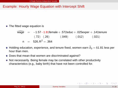
Holding education, experience, and tenure fixed, women earn bδ 0 = $1.81 less perhour than men.

Does that mean that women are discriminated against?

Not necessarily. Being female may be correlated with other productivitycharacteristics (e.g., baby birth) that have not been controlled for.



continue

Let’s compare means of subpopulations described by dummies:

\wage = 7.10�2.51female

(.21) (.30)

n = 526,R2 = .116 (< .364 as expected)

Not holding other factors constant, women earn $2.51 per hour less than men, i.e.the difference between the mean wage of men and that of women is $2.51.

Discussion:- It can easily be tested whether difference in means is significant,

jt j=��2.51.30

��= j�8.37j> 1.96.

- The wage difference between men and women is larger if no other things arecontrolled for; i.e. part of the difference is due to differences in education,experience and tenure between men and women.- When more factors (such as baby birth) are controlled for, then we expect bδ 0would be even smaller (until insignificance?).



Example: Effects of Training Grants on Hours of Training

The fitted regression line is

\hrsemp = 46.67+26.25grant� .98log(sales)�6.07log(employ)

(43.41)(5.59) (3.54) (3.88)

n = 105,R2 = .237

wherehrsemp = hours training per employee, at the firm levelgrant = dummy indicating whether firm received training grantemploy = number of employees

This is an example of program evaluation:- treatment group (= grant receivers) vs. control group (= no grant).- tgrant = 4.70> 1.96, but is the effect of treatment on the outcome of interestcausal? The answer depends on whether E [ujgrant ] = 0. It might be that to getgrants, some firms give more training to their employees.



a: Using Dummy Explanatory Variables in Equations for log(y)

Example (Housing Price Regression): The fitted regression line is

\log(price) = �1.35+ .168log(lotsize)+ .707log(sqrft)

(.65) (.038) (.093)

+.027bdrms+.054colonial

(.029) (.045)

n = 88,R2 = .649

wherecolonial = dummy for the colonial style [figure here]

Now,∂ log (price)

∂colonial=

∂price/price∂colonial

= 5.4%,

As the dummy for colonial style changes from 0 to 1, the house price increases by5.4 percentage points.



American Colonial Architecture

American colonial architecture includes several building design styles associatedwith the colonial period of the United States, including First Period English(late-medieval), French Colonial, Spanish Colonial, Dutch Colonial and Georgian.These styles are associated with the houses, churches and government buildingsof the period from about 1600 through the 19th century.

- From Wiki

Figure: Corwin House, Salem, Massachusetts, built about 1660, First Period English


Using Dummy Variables for Multiple Categories





1) Define membership in each category by a dummy variable;

2) Leave out one category (which becomes the base category).

Example (Log Hourly Wage Equation): The fitted regression line is

\log (wage) = �.321+.213marrmale�.198marrfem+

(.100)(.055) (.0058)

�.110singfem+ .079educ+ .027exper � .00054exper2

(.056) (.007) (.005) (.00011)

+.029tenure� .00053tenure2

(.007) (.00023)

n = 526,R2 = .461

Holding other things fixed, married women earn 19.8% less than single men (= thebase category); similarly, married men earn 21.3% more and single women earn11.0% (< 19.8%) less than single men. [economic intuition here]



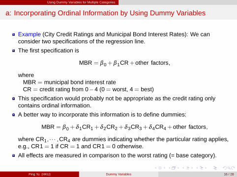
a: Incorporating Ordinal Information by Using Dummy Variables

Example (City Credit Ratings and Municipal Bond Interest Rates): We canconsider two specifications of the regression line.

The first specification is

MBR = β 0+β 1CR+other factors,

whereMBR = municipal bond interest rateCR = credit rating from 0�4 (0= worst, 4= best)

This specification would probably not be appropriate as the credit rating onlycontains ordinal information.

A better way to incorporate this information is to define dummies:

MBR = β 0+ δ 1CR1+ δ 2CR2+ δ 3CR3+ δ 4CR4+other factors,

where CR1, � � � ,CR4 are dummies indicating whether the particular rating applies,e.g., CR1= 1 if CR = 1 and CR1= 0 otherwise.

All effects are measured in comparison to the worst rating (= base category).



Difference Between These Two Specifications

Specification 1:

CR = 0=)MBR = β 0,

CR = 1=)MBR = β 0+β 1,

CR = 2=)MBR = β 0+2β 1,

CR = 3=)MBR = β 0+3β 1,

CR = 4=)MBR = β 0+4β 1,

where the increase in MBR for each rating improvement is the same - β 1.

Specification 2:

CR = 0=)MBR = β 0,

CR = 1=)MBR = β 0+ δ 1,

CR = 2=)MBR = β 0+ δ 2,

CR = 3=)MBR = β 0+ δ 3,

CR = 4=)MBR = β 0+ δ 4,

where the increase in MBR for each rating improvement can be different due tothe arbitrariness of δ 1, � � � ,δ 4.


Interactions Involving Dummy Variables




a: Interactions among Dummy Variables

Reconsider the female and marital status effect on log(wage) by adding thefemale �married interaction term:

\log (wage) = �.321� .110female+ .213married�.301female �married + � � �(.100) (.056) (.055) (.072)

marrmale: setting married = 1 and female = 0, we get bδ 2 = .213 as before.

marrfem: setting married = 1 and female = 1, we getbδ 1+bδ 2+

bδ 3 = �.110+ .213� .301= �.198 as before.

singfem: setting married = 0 and female = 1, we get bδ 1 = �.110 as before.

So these two specifications are equivalent: four categories are generated.

(*) What is the meaning of the coefficient of female �married , bδ 3?

(E [log (wage) jfemale = 1,married = 1]�E [log (wage) jfemale = 1,married = 0])

� (E [log (wage) jfemale = 0,married = 1]�E [log (wage) jfemale = 0,married = 0])

= [(δ 1+ δ 2+ δ 3)�δ 1]� [δ 2]

= difference (in gender) in difference (in marriage)

= difference (in marriage) in difference (in gender)



b: Allowing for Different Slopes

Consider the model

log (wage) = β 0+ δ 0female+β 1educ+ δ 1female �educ+u.

where

β 0 = intercept of men, β 1 = slope of men,

β 0+ δ 0 = intercept of women, β 1+ δ 1 = slope of women.

Interacting both the intercept and the slope with the female dummy enables one tomodel completely independent wage equations for men and women. [figure here]

Interesting Hypotheses:H0 : δ 1 = 0,

i.e., the return to education is the same for men and women, and

H0 : δ 0 = δ 1 = 0,

i.e., the whole wage equation is the same for men and women.



Figure: (a) δ 0 < 0,δ 1 < 0; (b) δ 0 < 0,δ 1 > 0



Example: Log Hourly Wage Equation

The fitted regression line is

\log (wage) = .389�.227female+ .082educ

(.119)(.168) (.008)

�.0056female �educ+ .029exper � .00058exper2

(.0131) (.005) (.00011)

+.032tenure� .00059tenure2

(.007) (.00024)

n = 526,R2 = .441

jtfemale�educ j=��.0056.0131

��= j�.43j< 1.96: No evidence against hypothesis that the

return to education is the same for men and women.jtfemalej=

��.227.168

��= j�1.35j< 1.96: Does this mean that there is no significant

evidence of lower pay for women at the same levels of educ, exper , and tenure?No: this is only the effect for educ = 0 since

∂ log (wage)∂ female

= �.227� .0056educ.



To answer the question one has to recenter the interaction term, e.g., aroundeduc = 12.5 (= average education) to have female � (educ�12.5):∂ log(wage)

∂ female = bδ 0+bδ 1 (educ�12.5) with new bδ 0 = �.297

0 12.5

0.162

0.389

1.117

1.414

malefemale

Figure: The New new bδ 0 = �.227+12.5� (�.0056) = �.297<�.227



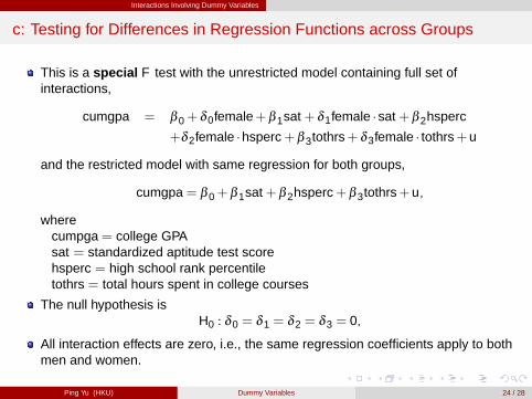
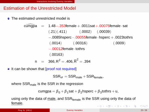
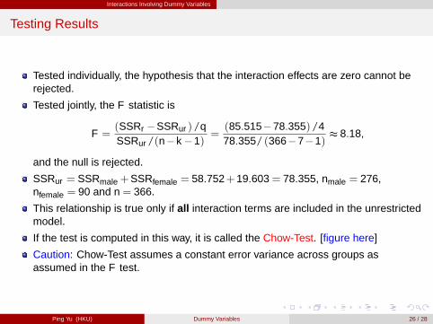
c: Testing for Differences in Regression Functions across Groups

This is a special F test with the unrestricted model containing full set ofinteractions,

cumgpa = β 0+ δ 0female+β 1sat+ δ 1female �sat+β 2hsperc

+δ 2female �hsperc+β 3tothrs+ δ 3female � tothrs+u

and the restricted model with same regression for both groups,

cumgpa= β 0+β 1sat+β 2hsperc+β 3tothrs+u,

wherecumpga= college GPAsat = standardized aptitude test scorehsperc = high school rank percentiletothrs = total hours spent in college courses

The null hypothesis isH0 : δ 0 = δ 1 = δ 2 = δ 3 = 0,

All interaction effects are zero, i.e., the same regression coefficients apply to bothmen and women.



Estimation of the Unrestricted Model

The estimated unrestricted model is

\cumgpa = 1.48�.353female+ .0011sat+.00075female �sat

(.21)(.411) (.0002) (.00039)

�.0085hsperc�.00055female �hsperc+ .0023tothrs

(.0014) (.00316) (.0009)

�.00012female � tothrs

(.00163)

n = 366,R2 = .406,R2= .394

It can be shown that [proof not required]

SSRur = SSRmale+SSRfemale,

where SSRmale is the SSR in the regression

cumgpa= β 0+β 1sat+β 2hsperc+β 3tothrs+u,

using only the data of male, and SSRfemale is the SSR using only the data offemale.



Testing Results

Tested individually, the hypothesis that the interaction effects are zero cannot berejected.

Tested jointly, the F statistic is

F =(SSRr �SSRur )/qSSRur /(n�k �1)

=(85.515�78.355)/478.355/ (366�7�1)

t 8.18,

and the null is rejected.

SSRur = SSRmale+SSRfemale = 58.752+19.603= 78.355, nmale = 276,nfemale = 90 and n = 366.

This relationship is true only if all interaction terms are included in the unrestrictedmodel.

If the test is computed in this way, it is called the Chow-Test. [figure here]

Caution: Chow-Test assumes a constant error variance across groups asassumed in the F test.



Gregory C. Chow (1929-), Princeton

Chow, G.C., 1960, Tests of Equality Between Sets of Coefficients in Two LinearRegressions, Econometrica, 28, 591-605.



Applications of the Chow-Test

Time Series: Structural Change Cross Section: Male vs. Female

Figure: Restricted and Unrestricted Models in the Chow Test

You must pass the Chow test to pass this course!


Date post:	21-May-2019
Category:	Documents
Upload:	duongminh
View:	217 times
Download:	0 times

Multiple Regression Analysis with Qualitative Information ...web.hku.hk/~pingyu/0701/Ch07_Dummy...

Documents