22
Lecture 15 1 Econ 140 Econ 140 Multiple Regression Applications Lecture 15
| Date post: | 31-Dec-2015 |
| Category: |
Documents |
| Upload: | jelani-underwood |
| View: | 15 times |
| Download: | 1 times |

Lecture 15 1
Econ 140Econ 140
Multiple Regression Applications
Lecture 15

Lecture 15 2
Econ 140Econ 140Today’s plan
• Relationship between R2 and the F-test.
• Restricted least squares and testing for the imposition of a linear restriction in the model

Lecture 15 3
Econ 140Econ 140R2
• We know
R2 Explained S of STotal S of S
• We can rewrite this as
Rb x y b x y
y2 1 1 2 2
2
^ ^
• Remember:
– If R2 = 1, the model explains all of the variation in Y
– If R2 = 0, the model explains none of the variation in Y
Lecture 15 4
Econ 140Econ 140R2 (2)
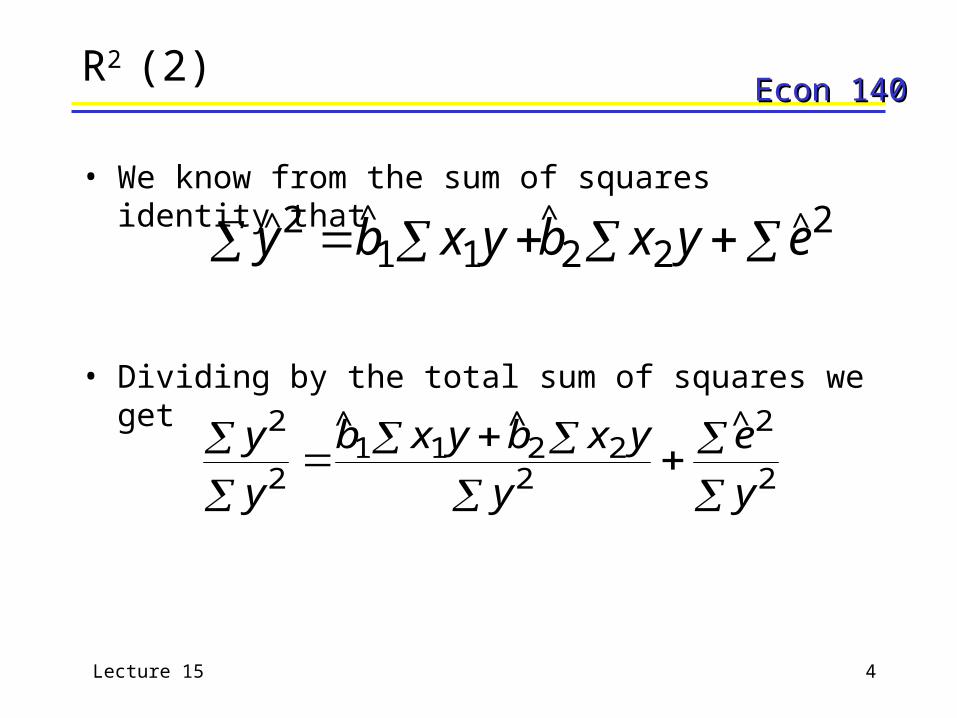
• We know from the sum of squares identity that
• Dividing by the total sum of squares we get
y b x y b x y e21 1 2 2
2 ^ ^ ^ ^
y
y
b x y b x y
y
e
y
2
21 1 2 2
2
2
2
^ ^ ^
Lecture 15 5
Econ 140Econ 140R2 (3)
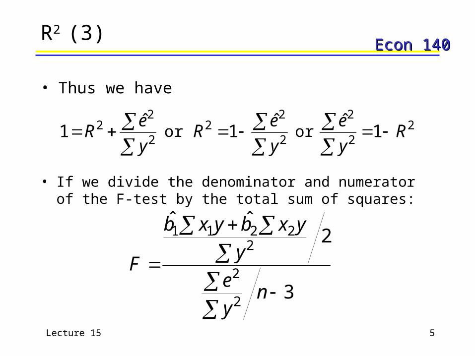
• Thus we have
2
22 ˆ
1y
eR
2
22 ˆ
1y
eR 2
2
2
1ˆ
Ry
e or or
• If we divide the denominator and numerator of the F-test by the total sum of squares:
3
2ˆˆ
2
2
22211
ny
e
y
yxbyxb
F

Lecture 15 6
Econ 140Econ 140F-stat in terms of R2
• Even if you’re not given the residual sum of squares, you can compute the F-statistic:
3)1(
22
2
nR
RF
• Recalling our LINEST (from L13.xls) output, we can substitute R2 = 0.188
– We would reject the null at a 5% significance level and accept the null at the 1% significance level
82.333188.01
2188.0
F

Lecture 15 7
Econ 140Econ 140Relationship between R2 & F
• When R2 = 0 there is no relationship between the Y and X variables
– This can be written as Y = a
– In this instance, we accept the null and F = 0
• When R2 = 1, all variation in Y is explained by the X variables
– The F statistic approaches infinity as the denominator would equal zero
– In this instance, we always reject the null

Lecture 15 8
Econ 140Econ 140Restricted Least Squares
• Imposing a linear restriction in a regression model and re-examining the relationship between R2 and the F-test.
• In restricted least squares we want to test a restriction such as
1:0 H
Where our model is
eKLaY lnlnln
• We can write = 1 - and substitute it into the model equation so that:
(lnY - lnK) = a + (lnL - lnK) + e

Lecture 15 9
Econ 140Econ 140Restricted Least Squares (2)
• We can rewrite our equation as: G = a +Z + e*
Where: G = (lnY - lnK) and Z = (lnL - lnK)
• The model with G as the dependent variable will be our restricted model – the restricted model is the equation we will estimate under the
assumption that the null hypothesis is true

Lecture 15 10
Econ 140Econ 140Restricted Least Squares (3)
• How do we test one model against another?
• We take the unrestricted and restricted forms and test them using an F-test
• The F statistic will be
kne
qeeF
2
2*2
ˆ
ˆˆ
– * refers to the restricted model
– q is the number of constraints
– in this case the number of constraints = 1 ( + = 1)
– n - k is the df of the unrestricted model

Lecture 15 11
Econ 140Econ 140Testing linear restrictions
• We wish to test the linear restriction imposed in the Cobb-Douglas log-linear model:
• Test for constant returns to scale, or the restriction:
H0: + = 1
• We will use L14.xls to test this restriction - worked out in L15.xls
eKLaY lnlnln

Lecture 15 12
Econ 140Econ 140Testing linear restrictions (2)
• The unrestricted regression equation estimated from the data is:
030.0 026.0 )185.0(
ln447.0ln674.0488.0ˆln eKLY
• Note the t-ratios for the coefficients:
: 0.674/0.026 = 26.01
: 0.447/0.030 = 14.98– compared to a t-value of around 2 for a 5% significance level, both & are very precisely determined
coefficients

Lecture 15 13
Econ 140Econ 140Testing linear restrictions (3)
– adding up the regression coefficients, we have:0.674 +0.447 = 1.121
– how do we test whether or not this sum is statistically different from 1?
• First, we rewrite the restriction: = 1- • Our restricted model is:
(lnY - lnK) = a + (lnL - lnK) + e
or
G = a +Z + e*
Lecture 15 14
Econ 140Econ 140Testing linear restrictions (4)
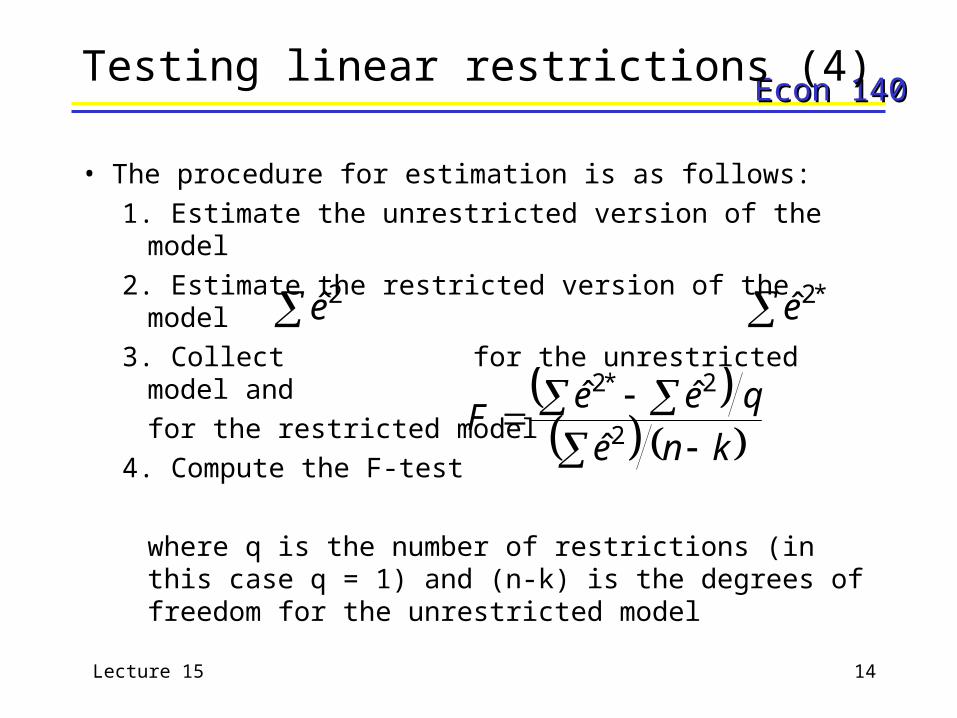
• The procedure for estimation is as follows:
1. Estimate the unrestricted version of the model
2. Estimate the restricted version of the model
3. Collect for the unrestricted model and
for the restricted model
4. Compute the F-test
where q is the number of restrictions (in this case q = 1) and (n-k) is the degrees of freedom for the unrestricted model
2e *2e
kne
qeeF
2
2*2
ˆ
ˆˆ

Lecture 15 15
Econ 140Econ 140Testing linear restrictions (5)
• On L15.xls we find a sample n = 32 and an estimated unrestricted model giving us the following information:
351.ˆ
996.0
030.0 026.0 )185.0(
ln447.0ln674.0488.0ˆln
2
2
e
R
eKLY

Lecture 15 16
Econ 140Econ 140Testing linear restrictions (7)
• The restricted model gives us the following information:
228.1ˆ
871.0R
(0.048) 1.061
679.0061.1ˆ
*2
2
e
ZG
• We can use this information to compute our F statistic:
F* = [(1.228 - 0.351)/1]/(0.359/29) = 72.47

Lecture 15 17
Econ 140Econ 140Testing linear restrictions (8)
• The F table value at a 5% significance level is:
F0.05,1,29 = 4.17
– Since F* > F0.05,1,29 we will reject the null hypothesis that there are constant returns to scale
• NOTE: the dependent variables for the restricted and unrestricted models are different
– dependent variable in unrestricted version: lnY
– dependent variable in restricted version: (lnY-lnK)
Lecture 15 18
Econ 140Econ 140Testing linear restrictions (9)
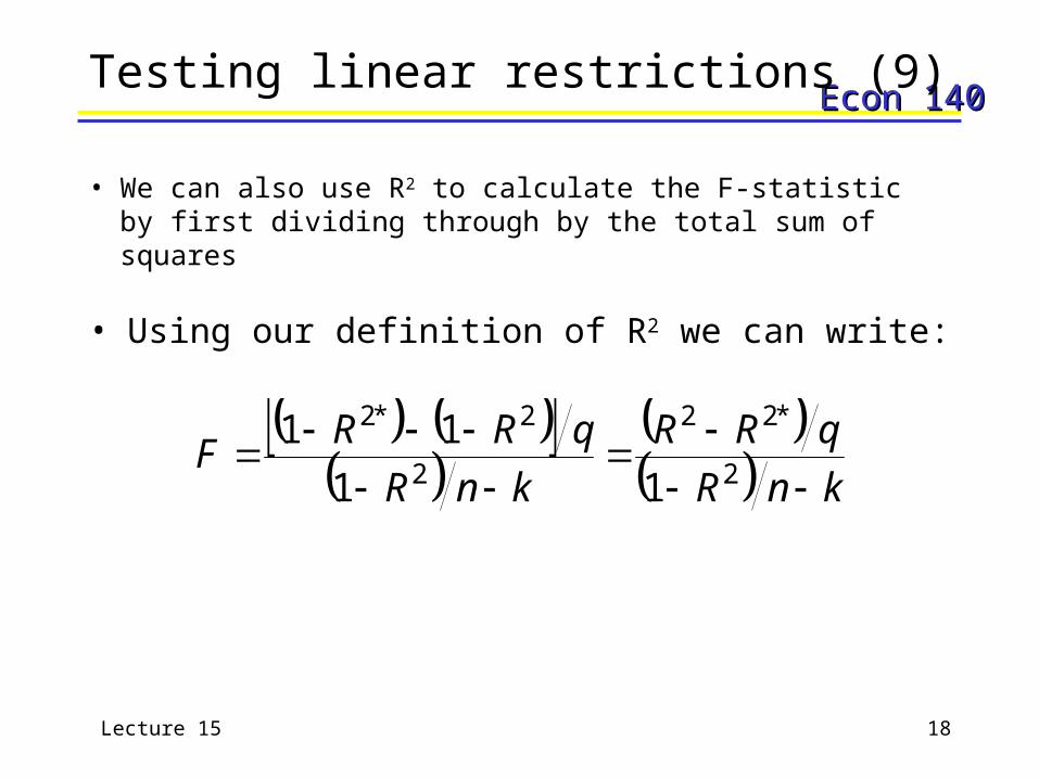
• We can also use R2 to calculate the F-statistic by first dividing through by the total sum of squares
• Using our definition of R2 we can write:
knR
qRR
knR
qRRF
2
*22
2
2*2
11
11

Lecture 15 19
Econ 140Econ 140Testing linear restrictions (10)
• NOTE: we cannot simply use the R2 from the unrestricted model since it has a different dependent variable
– What we need to do is take the expectation E(G|L,K)
• We need our unrestricted model to have the dependent variable G, or:
– Where G = (lnY - lnK)
– We can test this because we know that + - 1 = 0.121 since + = 1
– estimating this unrestricted model will give us the unrestricted R2
eKZaG ln1

Lecture 15 20
Econ 140Econ 140Testing linear restrictions (11)
• From L15.xls we have :
R2* = 0.871
R2 = 0.963
• Our computed F-statistic will be
47.72
0013.0
092.0
29963.01
1871.0963.0
F

Lecture 15 21
Econ 140Econ 140Testing linear restrictions (12)
• On L15.xls we have 32 observations of output, employment, and capital– The spreadsheet has regression output for the restricted and unrestricted models– The R2 and sum of squares are in bold type– F-tests on the restriction are on the bottom of the sheet
• We find that Excel gives us an F-statistic of 72.4665– The F table value at a 5% significance level is 4.1830– The probability that we would accept the null given this F-statistic is very small
Lecture 15 22
Econ 140Econ 140Testing linear restrictions (13)
• From this we can conclude that we have a model where there are increasing returns to scale. • We don’t know the true value, but we can reject the restriction that there are constant returns
to scale.


