Multiple stable reference points in oyster populations ...fishbull.noaa.gov/1072/powell2.pdf · 133...

133

All federal fisheries, and some state fisheries, are managed under biologi-cal reference-point guidelines under which a specific yearly allocation or quota is advised to constrain fishing mortality (e.g., Wallace et al.1). The biological reference-point approach for federal fisheries mandated by the Magnuson-Stevens Fishery Conser-vation and Management Act (Anony-mous, 1996) requires management of fish populations at a biomass that provides maximum sustainable yield. In this system, sophisticated survey, analytical, and modeling procedures are used to identify selected biological reference points, such as the target biomass, Bmsy, and the carrying capac-ity, K. Fishing mortality is then set in relation to reference point goals. Normally, Bmsy is defined in relation to carrying capacity, the biomass present without fishing, where natu-ral mortality balances recruitment (e.g., May et al., 1978; Johnson, 1994; Mangel and Tier, 1994; Rice, 2001). This stable point is characterized by a population for which most animals are adults, where natural mortality rates are low, and where recruitment is limited by compensatory processes such as resource limitation constrain-ing fecundity. Bmsy is most commonly defined as K

2, based on the well-known

Schaefer model that stipulates the

guiding premise that surplus pro-duction is highest at K

2 (Hilborn and Walters [1992]; see Restrepo et al. [1998] for more details on the federal management system).

The raison d’être for reference-point–based management is the de-velopment of equilibria between re-cruitment (and growth) and mortality at target host densities (the archetype being Bmsy). Unfortunately, for man-aging oyster populations, obstacles ex-ist in meeting this objective because oyster populations do not appear to be inherently equilibrious, particularly those subjected to MSX, a disease caused by the protozoan Haplospo-ridium nelsoni, or Dermo, a disease caused by the protozoan Perkinsus marinus. Time series of oyster abun-dance typically show wide interan-nual variations, mediated in no small measure by year-to-year differences in natural mortality rate, although overfishing has also been an impor-tant contributing agent (e.g., Mann et al., 1991; Rothschild et al., 1994; Burreson and Ragone Calvo, 1996; Ragone Calvo et al., 2001; Jordan et

Multiple stable reference points in oyster populations: implications for reference point-based management

Eric N. Powell (contact author)1

John M. Klinck2

Kathryn A. Ashton-Alcox1

John N. Kraeuter1

Email address for contact author: [email protected] Haskin Shellfish Research Laboratory Rutgers University 6959 Miller Ave. Port Norris, New Jersey 083492 Center for Coastal Physical Oceanography Crittenton Hall Old Dominion University Norfolk, Virginia 23529

Manuscript submitted 29 November 2007.Manuscript accepted 9 September 2008.Fish. Bull. 107:133–147 (2009).

The views and opinions expressed or implied in this article are those of the author and do not necessarily reflect the position of the National Marine Fisheries Service, NOAA.

Abstract—In the second of two com-panion articles, a 54-year time series for the oyster population in the New Jersey waters of Delaware Bay is analyzed to examine how the pres-ence of multiple stable states affects reference-point–based management. Multiple stable states are described by four types of reference points. Type I is the carrying capacity for the stable state: each has associ-ated with it a type-II reference point wherein surplus production reaches a local maximum. Type-II reference points are separated by an intermedi-ate surplus production low (type III). Two stable states establish a type-IV reference point, a point-of-no-return that impedes recovery to the higher stable state. The type-II to type-III differential in surplus production is a measure of the difficulty of rebuild-ing the population and the sensitivity of the population to collapse at high abundance. Surplus production pro-jections show that the abundances defining the four types of reference points are relatively stable over a wide range of uncertainties in recruitment and mortality rates. The surplus pro-duction values associated with type-II and type-III reference points are much more uncertain. Thus, biomass goals are more easily established than fishing mortality rates for oyster populations.

1 Wallace, R. K., W. Hosking, and S. T. Szedlmayer. 1994. Fisheries manage-ment for fishermen: A manual for help-ing fishermen understand the federal management process. NOAA MASG P-94-012, 56 p.

134 Fishery Bulletin 107(2)

Table 1The bed groups (by location: upbay and downbay) and subgroups (by mortality rate) for the eastern oyster (Crassostrea virginica) collected on twenty beds in Delaware Bay, as shown in Figure 1. Mortality rate divides each of the primary groups, themselves being divided by location, a surrogate for upbay-downbay vari-ations in dredge efficiency and fishery-area management regulations.

Bed group/subgroup Bed name

Upbay group Low mortality Round Island, Upper Arnolds,

Arnolds

Medium mortality Upper Middle, Middle, Sea Breeze, Cohansey, Ship John

Downbay group Medium mortality Shell Rock

High mortality Bennies Sand, Bennies, New Beds, Hog Shoal, Hawk’s Nest, Strawberry, Vexton, Ledge, Egg Island, Nantuxent Point, Beadons

al., 2002; Powell et al., 2008). In the first of two com-panion contributions, we described the case for oyster populations in Delaware Bay. A 54-year time series documents two regime shifts, circa-1970 and circa-1985, with intervening and succeeding intervals having the attributes of alternate stable states (sensu Gray, 1977; Peterson, 1984; Knowlton, 2004). Within these periods are substantial population excursions produced by vary-ing rates of recruitment and natural mortality, but the alternate stable states are demarcated by even larger excursions in abundance. Moreover, these periods of relative stability delineated by regime shifts are per-sistent and transcend a range of climatic conditions (Soniat et al., in press).

Population dynamics of the Delaware Bay oyster pop-ulation is not solely a function of disease, but stable-point abundances are at least partially a byproduct of disease, and disease has played a role in regime shifts (Powell et al., 2008). The classic view of carrying ca-pacity fails when disease accounts for a substantial fraction of natural mortality and this compromises an estimate of Bmsy. Some have attempted to redefine car-rying capacity in diseased populations in relation to the abundance (population density in classic disease models, e.g., Kermack and McKendrick [1991], Hethcote and van den Driessche [1995]) at which each diseased animal will produce, in its lifetime, a single infection event (e.g., Heesterbeek and Roberts, 1995; Swinton and Anderson, 1995). This abundance is always below, usually well below, the original K. When abundance rises above this level, the influence of disease increases, as does the chance of epizootic mortality. This increase restrains population abundance below the predisease K (e.g., Kermack and McKendrick, 1991; Hasiboder et al., 1992; Godfray and Briggs, 1995; Frank, 1996). This approach is not well tailored to diseases such as MSX and Dermo for which environment is a potent modu-lator of effect and in which rapid transmission rates are not requiring of host-to-host contact. Furthermore, the existence of multiple apparently stable states and regime shifts imply that the standard Schaefer model, from which such basic biological references points as Bmsy are derived, also does not provide the appropriate framework for managing oyster populations because this model has only a single stable state.

These ratiocinations lead to three salient questions pertinent to developing management goals for oyster stocks: 1) Can reference points be defined that consis-tently permit fishing without jeopardizing the sustain-ability of the stock? 2) Must management goals be set within the context of each of several multiple stable states? 3) How does regime change affect the usefulness of reference points and can management goals be set to increase the probability of regime shift to a preferred stable state? In this contribution, we use the case of the Delaware Bay oyster stock in New Jersey waters to examine these questions. In a companion contribution, we describe the long-term survey time series and the relationships of broodstock abundance with recruitment and mortality (Powell et al., 2009). In this contribu-

tion, we develop a surplus production model to relate these relationships with stock performance over a range of abundances. Following discussion of the results of simulations with this model, we consider the basis for an MSY-based management system for oyster popula-tions and the implications of multiple stable states in the decision-making process.

Model formulations and statistics

Powell et al. (2008, 2009) have provided an overview of the oyster populations in Delaware Bay during the 1953–2006 time period. Analyses of the Delaware Bay oyster resource of New Jersey routinely reveal a divi-sion between the upbay group of eight beds (Round Island, Upper Arnolds, Arnolds, Upper Middle, Middle, Sea Breeze, Cohansey, and Ship John [Fig. 1]) and the downbay group of twelve beds (Shell Rock, Bennies Sand, Bennies, New Beds, Nantuxent Point, Hog Shoal, Hawk’s Nest, Strawberry, Vexton, Beadons, Egg Island, and Ledge). Salinity, natural mortality rate, and growth rate are higher downbay. Dredge efficiencies are signifi-cantly higher downbay (Powell et al., 2002, 2007). Both regions can be subdivided on the basis of natural mortal-ity rate and productivity. In the upbay group, natural mortality rates and growth rates are significantly lower for the upper three beds, Round Island, Upper Arnolds and Arnolds, than for the remaining beds. Henceforth these two groups will be termed the low-mortality and medium-mortality beds (Table 1). In the downbay group, growth rates and mortality rates are lower for Shell Rock, leading to its designation as a medium-mortality bed; the reminder are high-mortality beds (Table 1).

135Powell et al.: Multiple stable reference points in oyster populations

Figure 1The twenty natural oyster beds of the eastern oyster (Crassostrea virginica) in the New Jersey waters of Delaware Bay may be characterized in terms of high-quality (dark shade) and medium-quality (light shade) grids. The term “quality” refers to a relative differential in long-term average oyster abundance (Powell et al, 2008). The footprints for the Middle bed (upper portion of figure) and the beds downbay from it, exceptNew Beds, Egg Island, and Ledge, were updated with data from surveys in 2005 and 2006. The footprints for the remaining beds were based on historical definitions.

Throughout this contribution, we will refer to these bay regions where necessary, but in general, we will model the entire stock. In the following section, we summarize the biological relationships identified by Powell et al. (2009) without further discussion.

Natural mortality fractions were obtained from box counts (bc) under the assumption that

N N Noysterst boxest liveoysterst−= +

1, (1)

where N = the number of individuals.

Hence,

Φbcboxest

boxest liveoysterst

N

N N=

+, (2)

where Φbc = the fraction of the individuals alive at the end of year t that died during the next year.


The fraction dead determined from box counts is re-lated to the natural mortality rate mbc as

mtbc

e bc= −−log ( )

,1 Φ

3)

where t = time.

Boxes do not adequately measure the mortality of juvenile animals. The fraction dying not recorded by box counts, Φ0, is obtained by difference:

ΦΦ Φ

01 1 1 1

1 1=

− − − −+

− − − −

− −

( ) ( )N N R N N

N Rt t t bc t f t

t t,, (4)

where Φf = the fraction taken by the fishery; R = the number of recruits into the population;

and the first parenthetical term on the right-hand side represents the difference in abun-dance between two consecutive surveys.

The two natural mortality rates, mbc (Eq. 3) and m0 (Eq. 5), are additive (sensu Hassell et al., 1982; Holmes, 1982), as the method for estimation includes the box counts as an input (Eq. 2) in contrast to fishing mortal-ity that can be compensatory under certain fishing sea-son scenarios (Klinck et al., 2001). Φ0 varied randomly over the time series with a 54-year mean of 0.274 and a 54-year median of 0.311 (Powell et al., 2008). The mortality rate can be obtained from Φ0 as

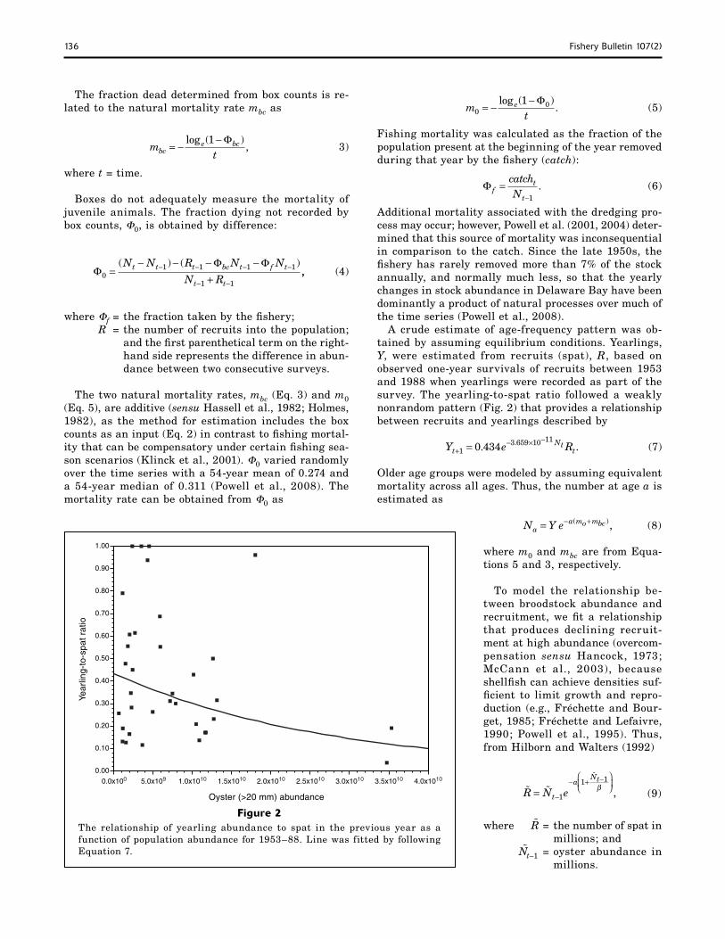
Figure 2The relationship of yearling abundance to spat in the previous year as a function of population abundance for 1953–88. Line was fitted by following Equation 7.

0.00

0.10

0.20

0.30

0.40

0.50

0.60

0.70

0.80

0.90

1.00

0.0x100 5.0x109 1.0x1010 1.5x1010 2.0x1010 2.5x1010 3.0x1010 3.5x1010 4.0x1010

Year

ling-

to-s

pat r

atio

Oyster (>20 mm) abundance

mt

e0

01= −

−log ( ).

Φ (5)

Fishing mortality was calculated as the fraction of the population present at the beginning of the year removed during that year by the fishery (catch):

Φ ft

t

catchN

=−1

. (6)

Additional mortality associated with the dredging pro-cess may occur; however, Powell et al. (2001, 2004) deter-mined that this source of mortality was inconsequential in comparison to the catch. Since the late 1950s, the fishery has rarely removed more than 7% of the stock annually, and normally much less, so that the yearly changes in stock abundance in Delaware Bay have been dominantly a product of natural processes over much of the time series (Powell et al., 2008).

A crude estimate of age-frequency pattern was ob-tained by assuming equilibrium conditions. Yearlings, Y, were estimated from recruits (spat), R, based on observed one-year survivals of recruits between 1953 and 1988 when yearlings were recorded as part of the survey. The yearling-to-spat ratio followed a weakly nonrandom pattern (Fig. 2) that provides a relationship between recruits and yearlings described by

Y e RtNt

t+− × −

=13 659 10 11

0 434. .. (7)

Older age groups were modeled by assuming equivalent mortality across all ages. Thus, the number at age a is estimated as

N Y eaa mo mbc= − +( ), (8)

where m0 and mbc are from Equa-tions 5 and 3, respectively.

To model the relationship be-tween broodstock abundance and recruitment, we fit a relationship that produces declining recruit-ment at high abundance (overcom-pensation sensu Hancock, 1973; McCann et al., 2003), because shellfish can achieve densities suf-ficient to limit growth and repro-duction (e.g., Fréchette and Bour-get, 1985; Fréchette and Lefaivre, 1990; Powell et al., 1995). Thus, from Hilborn and Walters (1992)

R N et

aNt

= −

− + −

1

1 1β , (9)

where R = the number of spat in millions; and

Nt–1 = oyster abundance in millions.


The recruitment rate Γt(Nt–1) is calculated as

Γt t

e

aNt

N

e

( )

log

−

− + −

=

+

1

1 1

1 β

tt. (10)

We compared the results of Equation 10 to that obtained for a best-fit linear regression with zero intercept. The linear relationship is

R Nt t= −0 493 1. . (11)

Note that the linear fit travels through the recruitment values at low abundance slightly below that traversed by the Ricker curve (Fig. 8 in Powell et al., 2009). Powell et al. (2009) provide caveats concerning the use of a single broodstock–recruitment curve for the population over the entire 54-yr time series. The dispersion of the stock over the four bay regions exerts limitations on the ambit of stock performance at any specific time.

Powell et al. (2009) develop an admittedly ad hoc em-pirical relationship to describe the relationship between box-count mortality and abundance:

Φbct e t

t t

Nt

N

N N e

= + +( ) −

+

−

− −

−− −

ω κ ρ

ϕ χ

log

1

1 1

1 ψψ

υ

)(

2

2 2

,

(12)

where ω =0.055, κ=0.03, ρ=1.0, ϕ=0.0025, χ=0.1, ψ=2.2, and υ= 0.8, with N expressed as billions of animals.

The specific mortality rate, mbc(N), is calculated with Equation 3. Equation 12 has the unique property of eliciting both depensatory and compensatory trends at low abundance. Powell et al. (2009) provide caveats concerning the use of the broodstock–mortality curve. The dispersion of the stock over the four bay regions exerts limitations on the ambit of stock performance at any specific time. At abundances greater than 4 × 109, mortality was low. The fraction dying each year aver-aged 9.6 % for these nonepizootic years, a nonepizootic year being defined for convenience as a year in which the fraction dying is less than 20%. However, of the 32 years with abundances less than 3 × 109, of which 14 were epizootic years, only one had a fractional mortal-ity between 0.15 and 0.20. Accordingly, two divergent outcomes exist over a range of low abundances. In some years, the fraction dying approximates the long-term mean for high-abundance years, about 9.6%. In other years, epizootic mortalities occur. The likelihood of these two divergent outcomes is substantively affected by the dispersion of the stock (Powell et al., 2009).

Surplus production S is calculated as the difference between additions to the population through recruit-ment and debits through mortality. The two processes are structurally uncoupled in time, however. First, mor-tality occurs differentially in time in relation to recruit-ment. Second, the method of data collection results in a time-integrated value of mortality, but a year ending value for recruitment, inasmuch as the death of recruits between settlement and the time of observation is not recognized as a component of the mortality term (see Keough and Downes, 1982; Powell et al., 1984; Caffey, 1985). Consequently, in the absence of fishing,

S N e t N et tt

tmbct m t t

= −( ) − −

− −

− +( )1 1

01 1Γ , (13)

which reduces to the familiar equation

S N e Rt tmbct mot t

t= +−− +( )

1 , (14)

where t = the time increment between observations of recruitment.

Note that the subscript t–1 is used for the stock abun-dance value N because the stock survey occurs at the end of the year preceding the year for which surplus production is forecast and for which recruitment is mea-sured.

Modeling of population dynamics—results of simulations and discussion

In the absence of fishing, the population increases when surplus production St is positive (Eq. 14). The popula-tion decreases when St is negative. Abundances where St is zero offer potential biological reference points, as do cases where St is maximal. Carrying capacity is an example of the former. In this case, mortality and recruitment balance and St=0. Surplus produc-tion declines as abundance nears carrying capacity and, therefore, the rate of change should be negative, but relatively constant; thus, dS

dN<0 and d S

dN

2

2~0. We will refer to reference points characterized by St=0, dSdN <0 and d S

dN

2

2~0 as type-I reference points (Fig. 3). Bmsy is defined to be a maximum in surplus production. Sur-plus production declines as abundance declines below or rises above this point. Hence, St>0, dS

dN=0 and d S

dN

2

2 <0. We will refer to maxima in surplus production as type-II reference points (Fig. 3). Because the time series under analysis is configured in terms of abundance rather than biomass, the designation Nmsy, rather than Bmsy, will be used hereafter.

We present hereafter a series of simulations of the Delaware Bay oyster stock designed to examine the change in surplus production with abundance. We first consider a population for which recruitment rate fol-lows Equation 9, a compensatory curve, with a 54-yr average unrecorded mortality rate (Eq. 5), and with the box-count mortality rate described by Equation 12.


Figure 3The trajectories of surplus production for cases detailed in Figures 4–7, with the locations of the four types of reference point indicated. Note that a type-IV reference point and two type-I reference points exist in only one case, Figure 7.

-0.8

-0.6

-0.4

-0.2

0.0

0.2

0.4

0.6

0.8

1.0

0 2 4 6 8 10 12

Figure 4

Figure 5

Figure 6

Figure 7

Zero rate of change

Type I

Type III

Type II Type II

Type IV

Type I

Sur

plus

pro

duct

ion

(bill

ions

)

Abundance (billions)

These relationships are depicted in Figures 7 and 10 of Powell et al. (2009). The trajectory for surplus pro-duction under these constraints is compared in Figure 3 and detailed in Figure 4. Recruitment rate rises as abundance declines (Fig. 4). This is anticipated from the compensation inherent in the relationship between broodstock and recruitment. The box-count mortal-ity rate shows a maximum somewhat above an abun-dance of 2 × 109 (Fig. 4). These relationships define a trend between surplus production and abundance that is divergent from the normal Schaefer curve (Ricker, 1975; Hilborn and Walters, 1992; Haddon, 2001; Zabel, 2003), as expected. The single type-I reference point is at N=9.3 × 109. This is an estimate of carrying capac-ity, K. Typically a single type-II reference point would exist, Nmsy, at about K

2, but in this case two maxima

in surplus production exist, one higher, NHmsy, than

the other, NLmsy. NH

msy is at N=4.86 × 109. This is the abundance classically interpreted as Nmsy, and, indeed, surplus production is maximal at this point and the value is approximately K

2 . The second type-II reference point occurs at N=1.43 × 109. Unlike the simple Schaefer curve depicted in Hilborn and Walters (1992), Haddon (2001), and Zabel (2003), a local minimum in surplus production exists between these two type-II surplus production maxima, at N=2.57 × 109. In this case, sur-plus production remains above zero, St>0. An increase in abundance above this level and a decrease in abun-dance below this level both increase surplus produc-tion. This reference point, herein designated type III,

always occurs between two maxima in surplus produc-tion and is characterized by dS

dN=0 and d S

dN

2

2> 0 (Table 2). The unusual nature of the surplus production curve in Figure 4, that yields the local minimum in surplus production and a secondary surplus production peak at a lower abundance, is produced by the depensatory and compensatory segments of the box-count mortality relationship established by the relationship between the occurrence of epizootics and abundance in the Delaware Bay oyster stock.

Figures 5–7 show three alternative trajectories for the change in surplus production with abundance in the Delaware Bay oyster stock obtained by small modi-fications of the parameters governing recruitment and mortality. The first is obtained by using the 54-yr me-dian unrecorded mortality rate, rather than the 54-yr mean rate. The median is distinctly higher. Again, the surplus production trajectory includes one type-I, two type-II, and one type-III reference points (Figs. 3 and 5). The abundance associated with the four refer-ence points remains unchanged, although the surplus production values associated with the type-II maxima and type-III minimum are lower than in the preceding case (Table 2).

The second alternative is obtained after a perusal of Figure 10 in Powell et al. (2009) that shows that the mortality rate for stock abundances frequented by epi-zootics often falls below the curve provided by Equation 12. This is a function of stock dispersion that modulates the likelihood of epizootic mortality rates (Powell et al.,

2009). In fact, on the average, box-count mortality rate reaches epizo-otic levels only half the time. Thus, Figures 3 and 6 show the trend in surplus production when epizoot-ics are assumed to occur only half the time, and box-count mortality rate is expressed as the average of a year with an epizootic and a year without one. The type-III reference point is nearer the NL

msy value in this surplus production trajectory, so that the valley between NL

msy and NH

msy is something more than a shoulder on the surplus production curve. Thus, the value of the sur-plus production maxima, averaged over a number of years, is strongly influenced by the frequency and in-tensity of epizootics (Table 2).

The final alternative addresses the uncertainty that exists in the shape of the broodstock–recruit-ment curve at low abundance. Linearizing the curve at low abun-dance (Eq. 11) yields a surplus production trajectory depicted in Figure 8 of Powell et al. (2009). The relationship is unique in gen-erating a second type-I reference


point, at N=1.93 × 109. This is a multiple-stable-point system with two carrying capacities, one at KH and one at KL. Note that the lower surplus production maximum is closer to KL than expected by the Schaefer relationship: NL

msy>K2 (Fig.

7). This representation of oyster population dynamics also gener-ates a type-IV reference point at N=3.03 × 109. Type IV, like type I, is characterized by St=0 and d S

dN

2

2 ~ 0, but in this case dS

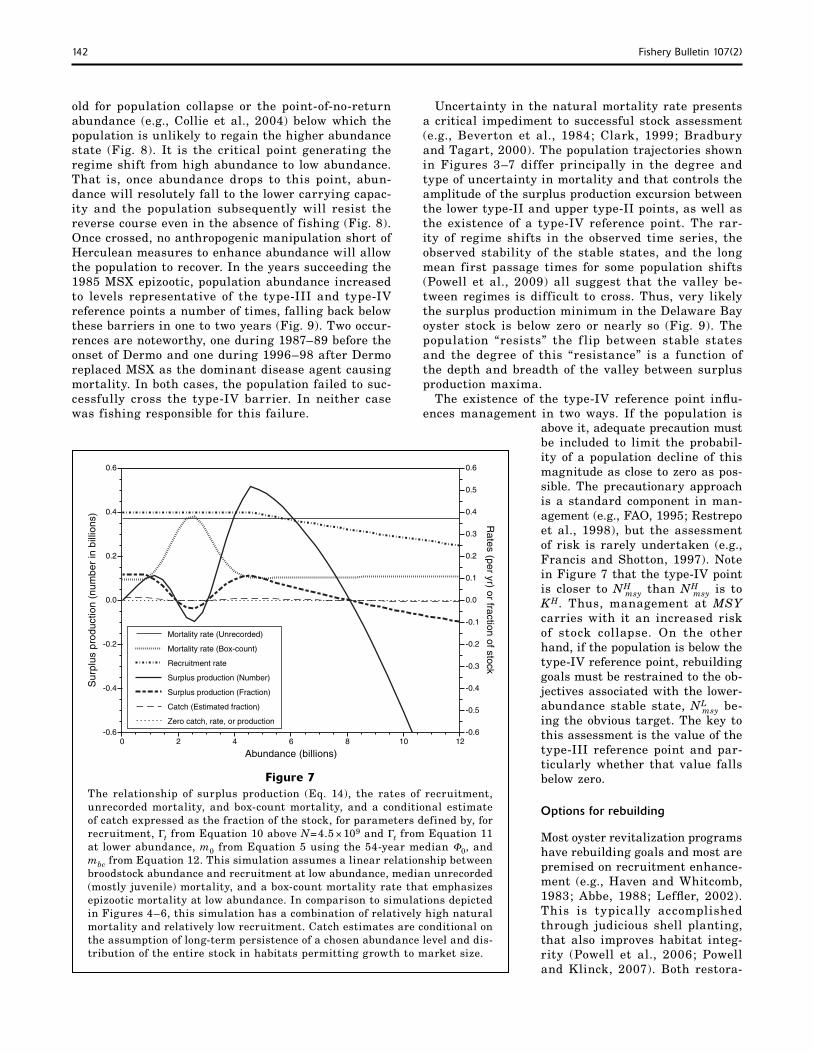
dN >0 (Table 2). Figure 8 presents a stylized version of the surplus production trajectory of Figure 7. Note that the type-I reference points are points of con-vergence. Abundance rising above this value will produce negative surplus production and a return to the abundance level and vice ver-sa for a decline in abundance. On the other hand, type-IV reference points are divergences or points of population instability. They mark thresholds for population collapse. The divergence that is the type-IV reference point is maintained by the competing rates of box-count mortality and recruitment that switch in dominance at this point (Fig. 8). A population reaching a type-IV reference point as abun-dance declines will see a rapid fur-ther decline. Once below this point, the likelihood becomes very low that the population can cross the gulf and re-acquire its high-abundance trajectory.

Reference-point–based management

Carrying capacity Perusal of the time series suggests that population abundances above about 12 × 109 are unstable. The analyses provided using Equation 14 return this same expectation, that carrying capacity is about 9.3 × 109. This explains the stability of population abundance during the 1970s as the population was at or near carrying capacity (Fig. 9). Abundance rose above this point a number of times between 1970 and 1985, but higher abundances were not sustainable. Interest-ingly, this carrying capacity is a carrying capacity for a population enzootic for MSX disease. The natural mortality rate during the 1970s is not much different from the few measures that exist for the time frame pre-1957 and the pre-MSX years are not outliers on the broodstock-recruitment diagram. So, MSX was not a significant agent of mortality during this period. Hence, predisease carrying capacity for which no empirical quantitative record exists is likely to have been similar to abundances during the 1970s, with the observed dif-

Figure 4The relationship of surplus production (Eq. 14), the rates of recruitment, unrecorded mortality, box-count mortality, and a conditional estimate of catch expressed as the fraction of the stock, for parameters defined by, for recruit-ment, Γt from Equation 10, m0 from Equation 5 using the 54-year average Φ0, and mbc from Equation 12. This simulation assumes compensation in the broodstock–recruitment curve, average unrecorded (mostly juvenile) mortal-ity, and a box-count mortality rate that emphasizes epizootic mortality at low abundance. Catch estimates are conditional on the assumption of long-term persistence of a chosen abundance level and distribution of the entire stock in habitats permitting growth to market size.

-0.6

-0.4

-0.2

0.0

0.2

0.4

0.6

0.8

-0.6

-0.5

-0.4

-0.3

-0.2

-0.1

0.0

0.1

0.2

0.3

0.4

0.5

0.6

0.7

0.8

0 2 4 6 8 10 12

Mortality rate (Unrecorded)

Mortality rate (Box-count)

Recruitment rate

Surplus production (Number)

Surplus production (Fraction)

Catch (Estimated fraction)

Zero catch, rate, or production

Sur

plus

pro

duct

ion

(num

ber

in b

illio

ns)


Rates (per yr) or fraction of stock

Table 2The surplus production values associated with the types I, II, III, and where applicable, IV reference points depicted in the referenced figures and the defining characteris-tics of each reference point type. Surplus production is expressed in billions of oysters. NA=not applicable.

Type I Type IV Carrying Type Type Type Point Figure capacity II III II of nonumber (K) NH

msy Smin NLmsy return

Surplus production 4 0.0 0.665 0.167 0.319 NA 5 0.0 0.511 0.103 0.275 NA 6 0.0 0.519 0.297 0.318 NA 7 0.0 0.511 –0.094 0.112 0.0

S dSdN d S

dN

2

2

Defining characteristics Type I =0 <0 ~0 Type II >0 =0 <0 Type III >0 or <0 =0 >0 Type IV =0 >0 ~0


Figure 5The relationship of surplus production (Eq. 14), the rates of recruitment, unrecorded mortality, and box-count mortality, and a conditional estimate of catch expressed as the fraction of the stock, for parameters defined by, for recruitment, Γt from Equation 10, m0 from Equation 5 using the 54-year median Φ0, and mbc from Equation 12. This simulation assumes compensation in the broodstock–recruitment curve, median unrecorded (mostly juvenile) mortality, and a box-count mortality rate that emphasizes epizootic mortality at low abundance. This simulation differs from the simulation in Figure 4 in a higher level of unrecorded mortality. Catch estimates are conditional on the assumption of long-term persistence of a chosen abundance level and distribu-tion of the entire stock in habitats permitting growth to market size.

-0.6

-0.4

-0.2

0.0

0.2

0.4

0.6

-0.6

-0.5

-0.4

-0.3

-0.2

-0.1

0.0

0.1

0.2

0.3

0.4

0.5

0.6

0 2 4 6 8 10 12



Recruitment rate





Sur

plus

pro

duct

ion

(num

ber

in b

illio

ns)



ferential in abundance in the 1950s primarily a result of the higher fishing mortality rates during that time.

Carrying capacity is defined by a set of criteria that are normally thought to be unique (Table 2). Inter-estingly, in Delaware Bay oyster populations, a sec-ond type-I reference point may exist, depending on the presence of a reference point of type IV, as considered subsequently. This type-I reference point, if present, is at 1.93 × 109, nearly a factor of 5 lower in abundance than the classic carrying capacity. However, this value is also similar to the abundance observed during the low-abundance phase of the population (Fig. 9), an out-come anticipated of a population with multiple stable points (Gray, 1977; Peterson, 1984) in which community compositions are theorized to resolve themselves into preferred states that can be exchanged only through triggering mechanisms capable of overcoming the iner-tia of the individual states. Soniat et al. (1998) argued that inertia is an important attribute of oyster popula-tion dynamics and that this inertia minimizes the in-fluence of short-term environmental shifts. The 54-year time series of Delaware Bay supports the importance of inertia and suggests some reasons for how population dynamics are internally stabilized.

Both recruitment and mortality have abundance-de-pendent rates. The high-abundance regime is inherently stable. Mean first passage times (sensu Rothschild and Mullen, 1985; Redner, 2001; Rothschild et al., 2005) for transitions to the alternate stable state typically exceed 6 yr (Powell et al., 2009). Given a population at high abundance: that population will tend to maintain itself because high abundance, on the average, gener-ates higher recruitment, and also, on the average, is associated with lower rates of natural mortality. Thus, high abundances have a strong internal self-sustain-ing mechanism. However, the 1970–85 period occurred prior to the onset of Dermo disease in Delaware Bay. Whether a high abundance state is sustainable under any environmental conditions with Dermo as the prin-cipal agent of mortality is unknown.

The low-abundance regime is stable only if the sur-plus production minimum separating the two maxima is negative. The differential between the two carrying capacities, KH and KL, is a factor of 4.82. Powell et al. (2009) discuss the tendency for the Delaware Bay oyster population to contract to a habitat of refuge on the me-dium-mortality beds (Table 1) as abundance falls. This occurs due to the gradient in natural mortality that

increasingly penalizes the popula-tion downestuary. The differential in bed area between the entire bay and the medium-mortality beds is a factor of 2.46 excluding the two lowermost and least produc-tive beds, Egg Island and Ledge, or 2.70 including them. Thus, habitat area, though likely a contributor to the differential in the two car-rying capacities, does not explain adequately the differential between KL and KH, and this agrees with the observation (Figure 5 in Powell et al., 2009) that contracted and dispersed population distributions both prevailed for extended periods during the low-abundance regime.

Surplus production targets Bever-ton et al. (1984) distinguish between short-term catch forecasts used to generate a yearly TAL and long-term strategic assessments used to set abundance goals. The constant-abundance reference point imple-mented with the model of Klinck et al. (2001) is particularly useful in maintaining a population close to an abundance target and has been used for short-term catch forecasts but does not lend itself to long-term strategic assessments. The purpose of this study was to develop refer-ence points that might be used to set abundance goals.


Figure 6The relationship of surplus production (Eq. 14), the rates of recruitment, unrecorded mortality, and box-count mortality, and a conditional estimate of catch expressed as the fraction of the stock, for parameters defined by, for recruitment, Γt from Equation 10, m0 from Equation 5 using the 54-year median Φ0, and mbc from Equation 12. This simulation assumes compensation in the broodstock–recruitment curve, median unrecorded (mostly juvenile) mortal-ity, but a box-count mortality rate that de-emphasizes epizootic mortality at low abundance. Epizootics are assumed to occur in half of the years when abundance is in the correct range, in comparison to the simulations shown in Figures 4 and 5. Surplus production as plotted is the average of an epizootic and a nonepizootic year. Catch estimates are conditional on the assumption of long-term persistence of a chosen abundance level and distribution of the entire stock in habitats permitting growth to market size.

-0.6

-0.4

-0.2

0.0

0.2

0.4

0.6

-0.6

-0.5

-0.4

-0.3

-0.2

-0.1

0.0

0.1

0.2

0.3

0.4

0.5

0.6

0 2 4 6 8 10 12



Recruitment rate





Sur

plus

pro

duct

ion

(num

ber

in b

illio

ns)



Four types of reference points are elucidated. Each of them marks critical spots in the ambit of oyster population dynamics that must be included in a successful management plan. If the oyster population in Delaware Bay has two distinct regimes, minimally, two sets of reference points ex-ist. It is a critical corollary of the multiple-stable-state theorem that such should be the case. Modern fisheries management scientists, although cognizant of the impor-tance of regime shifts, have not yet inculcated the concept of mul-tiple stable states into manage-ment philosophy and, consequent-ly, continue to focus solely on the highest abundance state.

Maximum sustainable yield gen- erally is considered to occur at half carrying capacity. For the high-abundance regime, NH

msy occurs at almost precisely K H

2 (Figs. 3–7),

as expected from standard fisher-ies theory (Haddon, 2001; Zabel et al., 2003). For the low-abundance regime, NL

msy occurs at a value dis-tinctly above K L

2; thus the lower

surplus production dome is dis-tinctly skewed. Some portion of this skewness may be inadequate extrapolation of the population dynamics to abundances below 0.8 × 109 that have not yet been observed. Either NH

msy or NLmsy

might be chosen as abundance goals. NH

msy yields the highest surplus production and, consequently, the highest fishery yield, and, all else being equal, would be the desirable goal for re-building oyster abundance above present-day levels. Over the 54-year time series for Delaware Bay, the abundance level has been near carrying capacity for about one-third of the years and well below NH

msy for most of the remaining years (Fig. 9). Thus, historical observations provide credence for the viability of this abundance goal.

However, an alternative exists, NLmsy. This second

type-II reference point exists at lower abundance and maximizes fishery yield in the low-abundance regime (Fig. 9). The population has been near this level for about two-thirds of the years since 1953 and, for most of this time, this population dynamic has been little inf luenced by fishing mortality. Thus, a substantive choice exists in managing the Delaware Bay oyster stock. Is it a viable choice to seek through management to transition the population to the high-abundance state and thereby rebuild the population to the higher NH

msy target?

The impact of type-III and type-IV reference points

The two other reference points become important at this juncture. The type-III reference point describes the valley between the two surplus production maxima. If negative, two stable states exist, asso-ciated with the lower and higher maxima in sur-plus production (e.g., Fig. 7). If positive, one stable state exists. The other lower maximum in surplus production is a quasi-stable state (e.g., Figs. 4–6). Surrounding the surplus production minimum is a region in which unwise harvest goals could create a region of negative surplus production and establish through overharvesting the second and lower stable state. Thus, this reference point is a measure of the relative degree of impedance present in the popula-tion dynamics to transiting to the higher stable state. This impedence exists naturally and is a rebuilding obstacle for management. This impedance can be deepened by inappropriate harvest goals.

If the minimum in surplus production is below zero, the type-IV reference point above it marks the thresh-


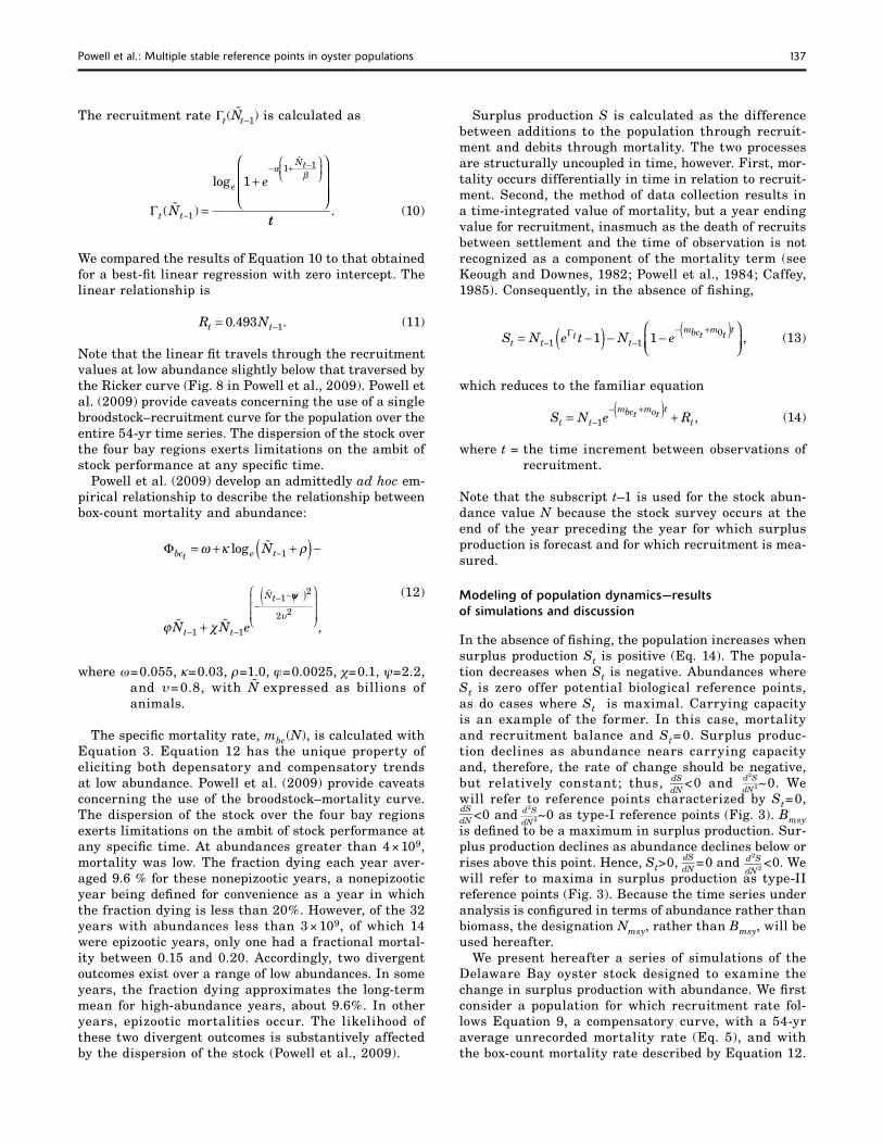
Figure 7The relationship of surplus production (Eq. 14), the rates of recruitment, unrecorded mortality, and box-count mortality, and a conditional estimate of catch expressed as the fraction of the stock, for parameters defined by, for recruitment, Γt from Equation 10 above N=4.5 × 109 and Γt from Equation 11 at lower abundance, m0 from Equation 5 using the 54-year median Φ0, and mbc from Equation 12. This simulation assumes a linear relationship between broodstock abundance and recruitment at low abundance, median unrecorded (mostly juvenile) mortality, and a box-count mortality rate that emphasizes epizootic mortality at low abundance. In comparison to simulations depicted in Figures 4–6, this simulation has a combination of relatively high natural mortality and relatively low recruitment. Catch estimates are conditional on the assumption of long-term persistence of a chosen abundance level and dis-tribution of the entire stock in habitats permitting growth to market size.

-0.6

-0.4

-0.2

0.0

0.2

0.4

0.6

-0.6

-0.5

-0.4

-0.3

-0.2

-0.1

0.0

0.1

0.2

0.3

0.4

0.5

0.6

0 2 4 6 8 10 12



Recruitment rate





Sur

plus

pro

duct

ion

(num

ber

in b

illio

ns)



old for population collapse or the point-of-no-return abundance (e.g., Collie et al., 2004) below which the population is unlikely to regain the higher abundance state (Fig. 8). It is the critical point generating the regime shift from high abundance to low abundance. That is, once abundance drops to this point, abun-dance will resolutely fall to the lower carrying capac-ity and the population subsequently will resist the reverse course even in the absence of fishing (Fig. 8). Once crossed, no anthropogenic manipulation short of Herculean measures to enhance abundance will allow the population to recover. In the years succeeding the 1985 MSX epizootic, population abundance increased to levels representative of the type-III and type-IV reference points a number of times, falling back below these barriers in one to two years (Fig. 9). Two occur-rences are noteworthy, one during 1987–89 before the onset of Dermo and one during 1996–98 after Dermo replaced MSX as the dominant disease agent causing mortality. In both cases, the population failed to suc-cessfully cross the type-IV barrier. In neither case was fishing responsible for this failure.

Uncertainty in the natural mortality rate presents a critical impediment to successful stock assessment (e.g., Beverton et al., 1984; Clark, 1999; Bradbury and Tagart, 2000). The population trajectories shown in Figures 3–7 differ principally in the degree and type of uncertainty in mortality and that controls the amplitude of the surplus production excursion between the lower type-II and upper type-II points, as well as the existence of a type-IV reference point. The rar-ity of regime shifts in the observed time series, the observed stability of the stable states, and the long mean first passage times for some population shifts (Powell et al., 2009) all suggest that the valley be-tween regimes is difficult to cross. Thus, very likely the surplus production minimum in the Delaware Bay oyster stock is below zero or nearly so (Fig. 9). The population “resists” the f lip between stable states and the degree of this “resistance” is a function of the depth and breadth of the valley between surplus production maxima.

The existence of the type-IV reference point influ-ences management in two ways. If the population is

above it, adequate precaution must be included to limit the probabil-ity of a population decline of this magnitude as close to zero as pos-sible. The precautionary approach is a standard component in man-agement (e.g., FAO, 1995; Restrepo et al., 1998), but the assessment of risk is rarely undertaken (e.g., Francis and Shotton, 1997). Note in Figure 7 that the type-IV point is closer to NH

msy than NHmsy is to

KH. Thus, management at MSY carries with it an increased risk of stock collapse. On the other hand, if the population is below the type-IV reference point, rebuilding goals must be restrained to the ob-jectives associated with the lower-abundance stable state, NL

msy be-ing the obvious target. The key to this assessment is the value of the type-III reference point and par-ticularly whether that value falls below zero.

Options for rebuilding

Most oyster revitalization programs have rebuilding goals and most are premised on recruitment enhance-ment (e.g., Haven and Whitcomb, 1983; Abbe, 1988; Leffler, 2002). This is typically accomplished through judicious shell planting, that also improves habitat integ-rity (Powell et al., 2006; Powell and Klinck, 2007). Both restora-


tion goals and methods have received consider-able attention (e.g., Breitburg et al., 2000; Mann, 2000).

Restoration goals are dramatically impacted by the location of type-II reference points in relation to stock abundance. Type II is the goal under MSY management objectives, and by the presence of type IV and the differential between types II and III. The difference between type II and type III affects 1) the ease of transition from one sta-ble point to another and 2) the impact on fishery yield during the transition. As the differential increases, from the example in the surplus pro-duction trajectory of Figure 6 to that in Figure 7 for instance, the limitation on fishery yield during the transition must increase. The obvious incon-gruity will be an observed increase in abundance of marketable stock during times of decreased al-location necessitated by the transitory limitation on surplus production coincident with the type-III reference point. This apparent inequity will likely exacerbate the natural adversarial relationship that exists between regulator and industry. The frequently complex relationship between economics and biology in fisheries management is well known (Lipton and Strand, 1992; Mackinson et al., 1997;

Figure 8The relationship of the primary trends in population abun-dance and surplus production associated with the bimodal surplus production trajectory depicted in Figure 7 in which the minimum in surplus production is negative. When surplus production is positive, the population abundance increases. The opposite trend occurs when surplus production is negative. The type-I reference point, the carrying capacity, is a conver-gence. Trends in surplus production and population abundance converge at this point. The type-IV reference point, the point of no return, is a divergence. Trends in surplus production and population abundance diverge at this point.

Sur

plus

pro

duct

ion

Population size

Neg

ativ

eP

ositi

ve0

Type 1

Type IV Type I

Imeson et al., 2002). Thus several questions come to the fore. Can rebuilding to NH

msy be accomplished? This depends on the existence of type IV. Does one try to re-build to NH

msy? This depends on the willingness of the f ishery and management to forgo catch yields during times of increasingly high abundance, possibly for an extended period, so that the population shifts to the higher regime.

Regime shifts of long-term stability almost cer-tainly come with a type-IV reference point. In this case, even the closure of the fishery will not gener-ate enough surplus pro-duction to rebuild past the type-III low. Recognizing the existence of such a bar-rier is critical. Presumably, a massive recruitment en-hancement program could be implemented to artifi-cially affect a regime shift. Patience may be the better alternative, using the Nmsy value of the present regime as the management goal

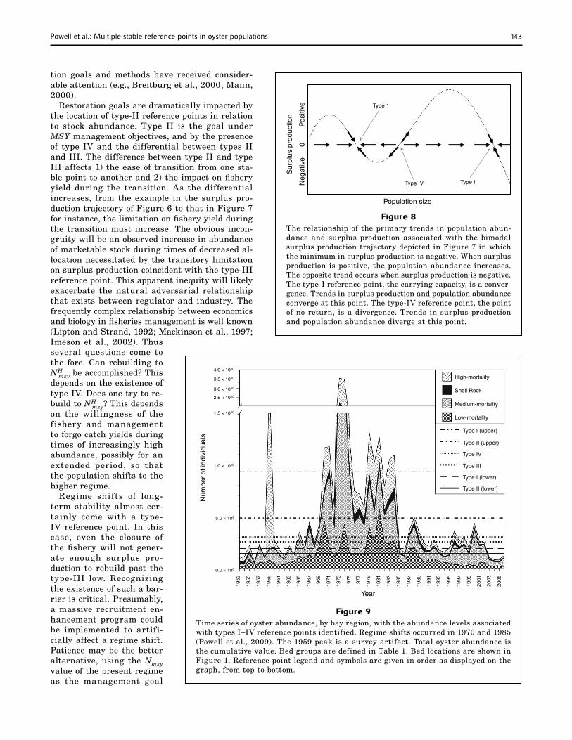
Figure 9Time series of oyster abundance, by bay region, with the abundance levels associated with types I–IV reference points identified. Regime shifts occurred in 1970 and 1985 (Powell et al., 2009). The 1959 peak is a survey artifact. Total oyster abundance is the cumulative value. Bed groups are defined in Table 1. Bed locations are shown in Figure 1. Reference point legend and symbols are given in order as displayed on the graph, from top to bottom.

Year

Num

ber

of in

divi

dual

s

High-mortality

Shell Rock

Medium-mortality

Low-mortality

Type I (upper)

Type II (upper)

Type IV

Type III

Type I (lower)

Type II (lower)

4.0 × 1010

3.5 × 1010

3.0 × 1010

2.5 × 1010

1.5 × 1010

1.0 × 1010

5.0 × 109

0.0 × 100

1953

1955

1957

1959

1961

1963

1965

1967

1969

1971

1973

1975

1977

1979

1981

1983

1985

1987

1989

1991

1993

1995

1997

1999

2001

2003

2005


while awaiting the rare sequence of events generating a natural transition to the alternate stable state.

Harvest goals

Included in Figures 4–7 is an estimated allowable catch as a fraction of the stock. The values of surplus produc-tion given in Figures 4–7 are expressed in numbers, perforce as they are the data source from which the underlying biological relationships are derived. The estimate is provided with some trepidation because the present model does not take into account the differential in growth across the salinity gradient and therefore tends to overestimate the number of animals of market size in the population as a whole. Moreover, the model assumes absolute constancy in the relationship of brood-stock to recruitment. Thus, the model may overestimate the fraction of the stock available for harvest in any given year. The formulation of Klinck et al. (2001) is a preferred option to obtain fishery allocations. Finally, the model consistently predicts a higher harvestable fraction at low abundance than at high abundance. An abettor in this trend may be the reliance of setting larvae more and more on the shell resource at low abundance than on the standing crop of living individuals. However, some portion of this outcome is likely due to an inability to accurately extrapolate the primary biological relation-ships below 0.8 × 109 animals. Such low abundances have not been observed and therefore the extrapolation is likely to be increasingly in error at lower and lower abundances. We do not give complete credence, therefore, to the proportional increase in harvestable fraction at low abundance indicated by the surplus production tra-jectories depicted in Figures 4–7.

From Figure 3 we observe that the range of abun-dances assigned to the various reference points varies little among simulations describing a range of assump-tions about natural mortality and recruitment rate. By contrast, the range of surplus production is pro-digious. Thus, an abundance goal distinguishing an overfished from a sustainable stock, e.g., Nmsy, is well constrained, whereas an overfishing definition, e.g., fmsy, is very poorly delimited. Clearly any successful approach to management must minimize the chance that the added mortality by fishing overcomes the in-ertia militating against abundance decline. Further, the uncertainty of the level of surplus production at its minimum and maxima (Fig. 5) necessitates precau-tion as the increased mortality from fishing may be sufficient to stabilize a quasi-stable state at low abun-dance. Both require, for oysters, that fishing mortality be maintained at a small percentage of the natural mortality rate, thereby permitting the inertia of the system to guard against an abundance decline and reducing the chance that a rare population expansion might be prematurely terminated. Even at Nmsy, fishing mortality rate is likely not to exceed 5–10% of the stock (Figs. 4–7). The history of the Delaware Bay fishery provides strong corroboration that removals exceed-ing 15% are not sustainable (Powell et al., 2008) and

offers strong evidence that removals below 5% of the stock limit the long-term impact of disease epizootics on abundance. Direct application of the Klinck et al. (2001) model in Delaware Bay has routinely returned values in the range of 1–3%. In addition, Powell and Klinck (2007) discuss the impact of fishing on the shell resource and the degradation of the shell beds upon which the population depends for its existence. That analysis independently argues for fishing mortality rates distinctly below the predisease mortality rate, at approximatly 10%.

It is noteworthy that allowable fishing mortality rates <10% of the stock are more similar to the mortality rates of the longest-lived bivalves, such as geoducks and ocean quahogs (e.g., Bradbury and Tagart, 2000; NEFSC2), than other species with life spans of the same order as the oyster, emphasizing the fact that oysters in the Mid-Atlantic region are much more akin in their population dynamics to long-lived k-selected species than to short lived r-selected ones.3 Low recruitment significantly restricts the ambit of the oyster’s popula-tion dynamics and significantly constrains allowable fishing mortality rates over a wide range of abundance values. A perusal of the broodstock-recruitment curve (Fig. 7 in Powell et al., 2009) shows that recruitment rate typically falls within the range of 0.25 to 1 spat per adult animal per year. Both this recruitment level and the <10%-per-year natural mortality rate is consistent with theoretical predisease generation times that likely exceeded 10 years (Mann and Powell, 2007) and the fact that reproduction continues to be consistent with an animal characterized by longer generation times.

Conclusions

The oyster population in Delaware Bay exhibits a popu-lation dynamics that is not normally described in com-mercial species. One reason is the presence of distinct and dynamically stable multiple stable points delimited by temporally rapid regime shifts. The result of this complexity is a series of reference points identified by the trajectory of surplus production, which departs dramati-cally from the simple Schaefer curve (e.g., Zabel et al., 2003). We define four reference point types in terms of surplus production, its derivative, and the rate of change of this derivative (Table 2). In Delaware Bay, the surplus production trajectory likely manifests two stable points and the carrying capacities associated with them and these agree relatively well with the observed stable

2 NEFSC (Northeast Fisheries Science Center). 2001. 33rd northeast regional stock assessment workshop (33rd SAW): Stock assessment review committee (SARC) consensus summary of assessments. NMFS NEFSC Ref. Doc. 01-18, 281 p.

3 Gulf of Mexico conditions with rapid growth (Ingle and Dawson, 1952; Butler, 1953; Hayes and Menzel, 1981) and multiple spawns per year (Hopkins, 1954; Hayes and Menzel, 1981; Choi et al., 1993, 1994) are examples of C. virginica under more r-selected conditions.


states in the population time series (Fig. 9). For each of these type-I reference points, a maximum in surplus production also exists. The presence of two stable states assures a type-III reference point that is a measure of the ease of transition between the two stable states and provides information on the likelihood that management can artificially impose a transition. In Delaware Bay, the type-III surplus production value may be negative. In this case, a type-IV reference point exists, a point-of-no-return. If the type-III reference point is positive, a quasi-stable state exists at low abundance that can be stabilized by overfishing. The existence of a positive type-III reference point imposes a particular conundrum to management in that rebuilding requires a reduction in fishery yield as abundance increases over a substan-tive abundance range.

The simulations show the uncertainty imposed by the limitations on accurate knowledge of the biological relationships. One noteworthy observation is that the location of the reference points undefined by a specific surplus production value (e.g., St=0), namely types II and III, are relatively stable in position with respect to population abundance over a wide range of uncertain-ties in recruitment and mortality rates (Table 2). The surplus production values associated with these refer-ence points are much more uncertain (Table 2). Thus, location is much better known than scale. As recom-mended by Beverton et al. (1984), different models are likely to be needed for short-term catch forecasts and estimation of abundance goals.

We describe reference points in the context of multiple stable states. The simplicity of the Bmsy–K couple so emphasized in fisheries management fails when mul-tiple stable states exist. That they may often exist is now well considered, although not yet inculcated into the oracle of fisheries management. Multiple stable points assure 1) that a type-III reference point exists, 2) that this point will impede the attainment of impru-dently formulated rebuilding goals, 3) that a type-IV point-of-no-return may exist that establishes a barrier to rebuilding, as well as imposing the conditions at high abundance necessary for stock collapse, and 4) that a carrying capacity may exist at abundances well below historically high abundances and well below the simplistic promulgation of Bmsy as half the carrying capacity established by the higher stable state. Use of the latter may impose impossible requirements for re-building a stock because the promulgated goal exceeds the carrying capacity for the controlling regime.

Acknowledgments

We recognize the many people who contributed over the years to the collection of the 54 years of survey data analyzed in this report, with particular recognition of the contributions by H. Haskin, D. Kunkle, and B. Richards. We appreciate the many suggestions on con-tent provided by S. Ford and D. Bushek. The study was funded by an appropriation from the State of New Jersey

to the Haskin Shellfish Research Laboratory, Rutgers University, and authorized by the Oyster Industry Sci-ence Steering Committee, a standing committee of the Delaware Bay Section of the Shell Fisheries Council of New Jersey.

Literature cited

Abbe, G. R. 1988. Population structure of the American oyster,

Crassostrea virginica, on an oyster bar in central Chesa-peake Bay: Changes associated with shell planting and increased recruitment. J. Shellfish Res. 7:33–40.

Anonymous. 1996. Magnuson-Stevens Fishery Conservation and Man-

agement Act. NOAA Tech. Memo. NMFS-F/SPO-23, 121 p.

Beverton, R. J. H., J. G. Cooke, J. B. Csirke, R. W. Doyle, G. Hempel, S. J. Holt, A. D. MacCall, D. J. Policansky, J. Roughgarden, J. G. Shepherd, M. P. Sissenwine, and P. H. Wiebe.

1984. Dynamics of single species group report. In Exploi-tation of marine communities (R. M. May, ed.), p. 13–58. Dahlem Konferenzen, Springer-Verlag, Berlin.

Bradbury, A., and J. V. Tagart.2000. Modeling geoduck, Panopea abrupta (Conrad, 1849)

population dynamics II. Natural mortality and equilib-rium yield. J. Shellfish Res. 19:63–70.

Breitburg, D. L., L. D. Coen, M. W. Luckenbach, R. Mann, M. Posey, and J. A. Wesson.

2000. Oyster reef restoration: Convergence of harvest and conservation strategies. J. Shellfish Res. 19:371–377.

Burreson, E. M., and L. M. Ragone Calvo 1996. Epizootiology of Perkinsus marinus disease of oys-

ters in Chesapeake Bay, with emphasis on data since 1985. J. Shellfish Res. 15:17–34.

Butler, P. A. 1953. Oyster growth as affected by latitudinal tempera-

ture gradients. Commer. Fish Rev. 15:7–12.Caffey, H. M.

1985. Spatial and temporal variation in settlement and recruitment of intertidal barnacles. Ecol. Monogr. 55:313–332.

Choi, K-S., D. H. Lewis, E. N. Powell, and S. M. Ray. 1993. Quantitative measurement of reproductive

output in the American oyster, Crassostrea virginica (Gmelin), using an enzyme-linked immunosorbent assay (ELISA). Aquacult. Fish. Manag. 24:299–322.

Choi, K-S., E. N. Powell, D. H. Lewis, and S. M. Ray. 1994. Instantaneous reproductive effort in female Ameri-

can oysters, Crassostrea virginica, measured by a new immunoprecipitation assay. Biol. Bull. (Woods Hole) 186:41–61.

Clark, W. G. 1999. Effects of an erroneous natural mortality rate

on a simple age-structured stock assessment. Can. J. Fish. Aquat. Sci. 56:1721–1731.

Collie, J. S., K. Richardson, and J. H. Steele. 2004. Regime shifts: Can ecological theory illuminate

the mechanisms? Prog. Oceanogr. 60:281–302.FAO (Food and Agriculture Organization of the United Nations).

1995. Technical consultation on the precautionary approach to capture fisheries. Precautionary approach


to f isheries. Part 1: Guidelines on the precaution-ary approach to capture fisheries and species intro-ductions. FAO Fisheries Tech. Pap. no. 350, part A, 52 p. FAO, Rome.

Francis, R. I. C. C., and R. Shotton. 1997. “Risk” in fisheries management: A review. Can.

J. Fish. Aquat. Sci. 54:1699–1715.Frank, S. A.

1996. Models of parasite virulence. Q. Rev. Biol. 71:37–78.

Fréchette, M., and E. Bourget. 1985. Food-limited growth of Mytilus edulis L. in relation

to the benthic boundary layer. Can. J. Fish. Aquat. Sci. 42:1166–1170.

Fréchette, M., and D. Lefaivre. 1990. Discriminating between food and space limita-

tion in benthic suspension feeders using self-thinning relationships. Mar. Ecol. Prog. Ser. 65:15–23.

Godfray, H. C. J., and C. J. Briggs. 1995. The population dynamics of pathogens that control

insect outbreaks. J. Theor. Biol. 176:125–136.Gray, J. S.

1977. The stability of benthic ecosystems. Helgol. Wiss. Meeresunters. 30:427–444.

Haddon, M. 2001. Modelling and quantitative methods in fisheries,

406 p. Chapman and Hall, Boca Raton, FL.Hancock, D. A.

1973. The relationship between stock and recruitment in exploited invertebrates. Rapp. P-v. Réun Cons. Int. Explor. Mer 164:113–131.

Hasiboder, G., C. Dye, and J. Carpenter.1992. Mathematical modelling and theory for esti-

mating the base reproduction number of canine leishmaniasis. Parasitology 105:43–53.

Hassell, M. P., R. C. Anderson, J. E. Cohen, B. Cujetanovic, A. P. Dobson, D. E. Gill, J. C. Holmes, R. M. May, T. McKeown, and M. S. Pereira.

1982. Impact of infectious diseases on host populations. In Population biology of infectious diseases (R. M. Anderson, and R. M. May, eds.), p. 15–35. Dahlem Konferenzen, Springer-Verlag, New York, NY.

Haven, D. S., and J. P. Whitcomb. 1983. The origin and extent of oyster reefs in the James

River, Virginia. J. Shellfish Res. 3:141–151.Hayes, P. F., and R. W. Menzel.

1981. The reproductive cycle of early setting Crassostrea virginica (Gmelin) in the northern Gulf of Mexico, and its implications for population recruitment. Biol. Bull. (Woods Hole) 160:80–88.

Heesterbeek, J. A. P., and H. G. Roberts. 1995. Mathematical models for microparasites of

wildlife. In Ecology of infectious diseases in natural populations (B. T. Grenfell, and A. P. Dobson, eds.), p. 90–122. Cambridge Univ. Press, Cambridge, UK.

Hethcote, H. W., and P. van den Driessche. 1995. An SIS epidemic model with variable population

size and a delay. J. Math. Biol. 34:177–194.Hilborn, R., and C. J. Walters.

1992. Quantitative fisheries stock assessment. Choice, dynamics and uncertainty, 570 p. Chapman and Hall, New York, NY.

Holmes, J. C. 1982. Impact of infectious disease agents on the population

growth and geographical distributions of animals. In Population biology of infectious diseases (R. M. Anderson,

and R. M. May, eds.), p. 37–51. Dahlem Konferenzen, Springer-Verlag, New York, NY.

Hopkins, S. H. 1954. Oyster setting on the Gulf coast. Proc. Natl.

Shellfish. Assoc. 45:52–55.Imeson, R. J., J. C. J. M. van den Bergh, and J. Hoekstra.

2002. Integrated models of fisheries management and policy. Environ. Model. Assess. 7:259–271.

Ingle, R. M., and C. E. Dawson Jr. 1950. Variation in salinity and its relation to the Florida

oyster. Part One: Salinity variations in Apalachicola Bay. Proc. Natl. Shellfish. Assoc. p. 6–19.

Johnson, L. 1994. Pattern and process in ecological systems: A step

in the development of a general ecological theory. Can. J. Fish. Aquat. Sci. 51:226–246.

Jordan, S. J., K. N. Greenhawk, C. B. McCollough, J. Vanisko, and M. L. Homer

2002. Oyster biomass, abundance, and harvest in north-ern Chesapeake Bay: Trends and forecasts. J. Shellfish Res. 21:733–741.

Keough, M. J., and B. J. Downes. 1982. Recruitment of marine invertebrates: The role of

active larval choices and early mortality. Oecologia (Berl.) 54:348–352.

Kermack, W. O., and A. G. McKendrick. 1991. Contributions to the mathematical theory of epi-

demics—I. Bull. Math. Biol. 53:33–55.Klinck, J. M., E. N. Powell, J. N. Kraeuter, S. E. Ford, and K. A.

Ashton-Alcox. 2001. A fisheries model for managing the oyster fish-

ery during times of disease. J. Shellfish Res. 20:977–989.

Knowlton, N.2004. Multiple “stable” states and the conservation of

marine ecosystems. Prog. Oceanogr. 60:387–396.Leffler, M.

2002. Crisis and controversy. Does the bay need a new oyster? Chesapeake Quart. 1:2–9.

Lipton, D. W., and I. E. Strand. 1992. Effect of stock size and regulations on fishing indus-

try cost and structure: The surf clam industry. Am. J. Agr. Econ. 74:197–208.

Mackinson, S., U. R. Sumaila, and T. J. Pitcher. 1997. Bioeconomics and catchability: Fish and fishers

behaviour during stock collapse. Fish. Res. 31:11–17.

Mangel, M., and C. Tier. 1994. Four facts every conservation biologist should know

about persistence. Ecology 75:607–614.Mann, R.

2000. Restoring the oyster reef communities in the Chesapeake Bay: A commentary. J. Shellfish Res. 19:335–339.

Mann, R., E. M. Burreson, and P. K. Baker. 1991. The decline of the Virginia oyster f ishery in

Chesapeake Bay: Considerations for the introduction of a non-endemic species, Crassostrea gigas (Thunberg, 1793). J. Shellfish Res. 10:379–388.

Mann, R., and E. N. Powell. 2007. Why oyster restoration goals in the Chesapeake Bay

are not and probably cannot be achieved. J. Shellfish Res. 26:905–917.

May, R. M., J. R. Beddington, J. W. Horwood, and J. G. Shepherd. 1978. Exploiting natural populations in an uncertain

world. Math. Biosci. 42:219–252.


McCann, K. S., L. W. Botsford, and A. Hasting.2003. Differential response of marine populations to cli-

mate forcing. Can. J. Fish. Aquat. Sci. 60:971–985.Peterson, C. H.

1984. Does a rigorous criterion for environmental identity preclude the existence of multiple stable points? Am. Nat. 124:127–133.

Powell, E. N., and K. A. Ashton-Alcox. 2004. A comparison between a suction dredge and a tra-

ditional oyster dredge in the transplantation of oysters in Delaware Bay. J. Shellfish Res. 23:803–823.

Powell, E. N., K. A. Ashton-Alcox, S. E. Banta, and A. J. Bonner.

2001. Impact of repeated dredging on a Delaware Bay oyster reef. J. Shellfish Res. 20:961–975.

Powell, E. N., K. A. Ashton-Alcox, J. A. Dobarro, M. Cummings, and S. E. Banta.

2002. The inherent efficiency of oyster dredges in survey mode. J. Shellfish Res. 21:691–695.

Powell, E. N., K. A. Ashton-Alcox, and J. N. Kraeuter.2007. Reevaluation of eastern oyster dredge efficiency

in survey mode: Application in stock assessment. N. Am. J. Fish. Manag. 27:492–511.

Powell, E. N., K. A. Ashton-Alcox, J. N. Kraeuter, S. E. Ford, and D. Bushek.

2008. Long-term trends in oyster population dynam-ics in Delaware Bay: Regime shifts and response to disease. J. Shellfish Res. 27:729–755.

Powell, E. N., H. Cummins, R. J. Stanton Jr., and G. Staff.1984. Estimation of the size of molluscan larval settle-

ment using the death assemblage. Estuarine Coastal Shelf Sci. 18:367–384.

Powell, E. N., and J. M. Klinck.2007. Is oyster shell a sustainable estuarine resource? J.

Shellfish Res. 26:181–194.Powell, E. N., J. M. Klinck, K. A. Ashton-Alcox, J. N. Kraeuter.

2009. Multiple stable reference points in oyster popu-lations: biological relationships for the eastern oyster (Crassostrea virginica) in Delaware Bay. Fish. Bull. 107:109–132.

Powell, E. N., J. M. Klinck, E. E. Hofmann, E. A. Wilson-Ormond, and M. S. Ellis.

1995. Modeling oyster populations. V. Declining phyto-plankton stocks and the population dynamics of Ameri-can oyster (Crassostrea virginica) populations. Fish. Res. 24:199–222.

Powell, E. N., J. N. Kraeuter, and K. A. Ashton-Alcox.2006. How long does oyster shell last on an oyster

reef? Estuarine Coastal Shelf Sci. 69:531–542.Ragone Calvo, L. M., R. L. Wetzel, and E. M. Burreson

2001. Development and verification of a model for the

population dynamics of the protistan parasite, Per-kinsus marinus, within its host, the eastern oyster, Crassostrea virginica, in Chesapeake Bay. J. Shellfish Res. 20:231–241.

Redner, S. 2001. A guide to first-passage processes, 312 p. Cam-

bridge Univ. Press, Cambridge, U.K.Restrepo, V. R., G. G. Thompson, P. M. Mace, W. K. Gabriel, L. L.

Low, A. D. MacCall, R. D. Methot, J. E. Powers, B. L. Taylor, P. R. Wade, and J. F. Witzig.

1998. Technical guidance on the use of precautionary approaches to implementing National Standard 1 of the Magnuson/Stevens Fishery Conservation and Man-agement Act. NOAA Tech. Memo. NMFS-F/SPO-31, 54 p.

Rice, J. 2001. Implications of variability on many time scales for

scientific advice on sustainable management of living marine resources. Prog. Oceanogr. 49:189–209.

Ricker, W. E. 1975. Computation and interpretation of biological sta-

tistics of fish populations. Bull. Fish. Res. Board Can. 191:1–382.

Rothschild, B. J., J. S. Ault, P. Goulletquer, and M. Héral 1994. Decline of the Chesapeake Bay oyster populations:

A century of habitat destruction and overfishing. Mar. Ecol. Prog. Ser. 111:29–39.

Rothschild, B. J., C. Chen, and R. G. Lough. 2 0 0 5 . M a n a g i n g f i sh s t o ck s u nder c l i m at e

uncertainty. ICES J. Mar. Sci. 62:1531–1541.Rothschild, B. J., and A. J. Mullen.

1985. The information content of stock-and-recruitment data and non-parametric classification. J. Cons. Int. Explor. Mer. 42:116–124.

Soniat, T. M., E. N. Powell, E. E. Hofmann, and J. M. Klinck.1998. Understanding the success and failure of oyster

populations: The importance of sampled variables and sample timing. J. Shellfish Res. 17:1149–1165.

Soniat, T. M., E. N. Powell, J. M. Klinck, and E. E. Hofmann. In press. Understanding the success and failure of oyster

populations: Climatic cycles and Perkinsus marinus. Int. J. Earth Sci.

Swinton, J., and R. M. Anderson. 1995. Model frameworks for plant-pathogen inter-

actions. In Ecology of infectious diseases in natural populations (B. T. Grenfell, and A. P. Dobson, eds.), p. 280–294. Cambridge Univ. Press, Cambridge, U.K.

Zabel, R. W., C. J. Harvey, S. L. Katz, T. P. Good, and P. S. Levin.

2003. Ecologically sustainable yield. Am. Sci. 91:150–157.

Date post:	29-Jul-2018
Category:	Documents
Upload:	phamthien
View:	214 times
Download:	0 times

Multiple stable reference points in oyster populations ...fishbull.noaa.gov/1072/powell2.pdf · 133...

Documents