Multiscale Computation for Incompressible Flow and Transport Problems Thomas Y. Hou Applied Mathematics, Caltech Collaborators: Y. Efenidev (TAMU), V. Ginting (Colorado), T. Strinopolous (Caltech), Danping Yang (ShandongUniv.), H. Ran (Caltech) Multiscale Computation for Incompressible Flow and Transport Problems – p.1/66
Transcript
Multiscale Computation for Incompressible Flow andTransport Problems
Thomas Y. Hou
Applied Mathematics, Caltech
Collaborators: Y. Efenidev (TAMU), V. Ginting (Colorado),
T. Strinopolous (Caltech), Danping Yang (Shandong Univ.), H. Ran (Caltech)
Multiscale Computation for Incompressible Flow and Transport Problems – p.1/66
Introduction
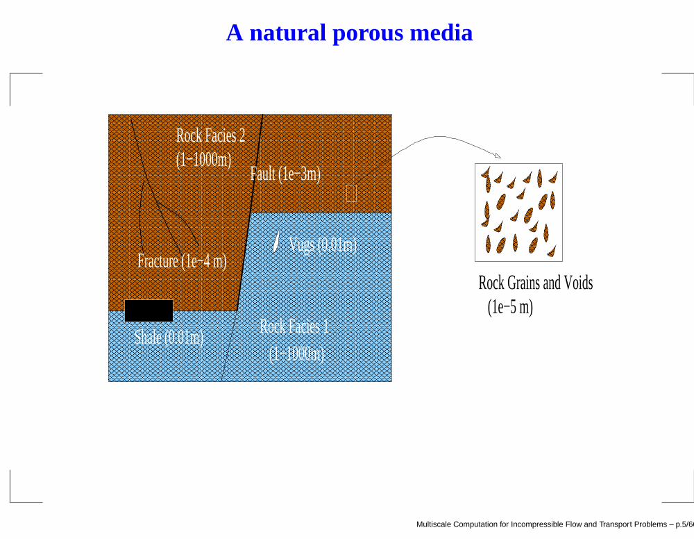
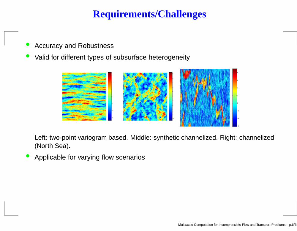
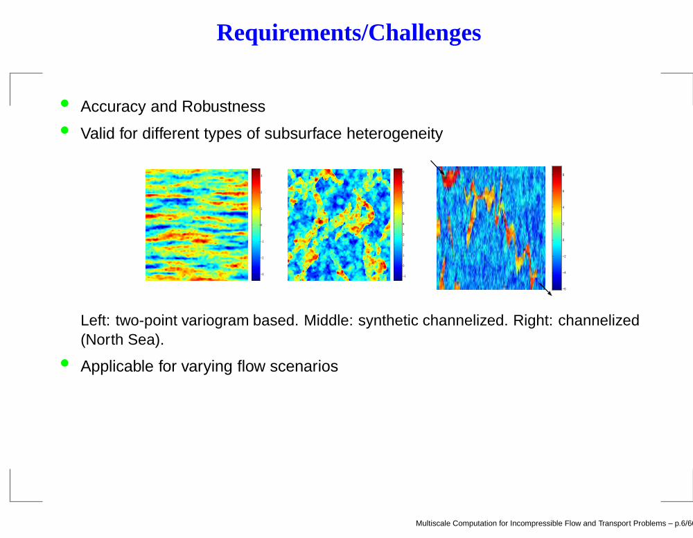
• Subsurface flows and transport are affected by heterogeneities at multiple scales(pore scale, core scale, field scale).
• Because of wide range of scales direct numerical simulations are not affordable.
• Upscaling of flow and transport parameters is commonly used in practice.
• Multiscale approaches are developed as an alternative to perform upscaling in thesolution space.
Multiscale Computation for Incompressible Flow and Transport Problems – p.2/66
Outline
• Multiscale finite element methods (MsFEM) as a subgrid modeling technique;
• Applications of multiscale finite element methods to porous media flows;
• Upscaling of two-phase flow in flow-based coordinate system;
• Multiscale computation for the Navier-Stokes equations;
Multiscale Computation for Incompressible Flow and Transport Problems – p.3/66
Darcy’s law and permeability
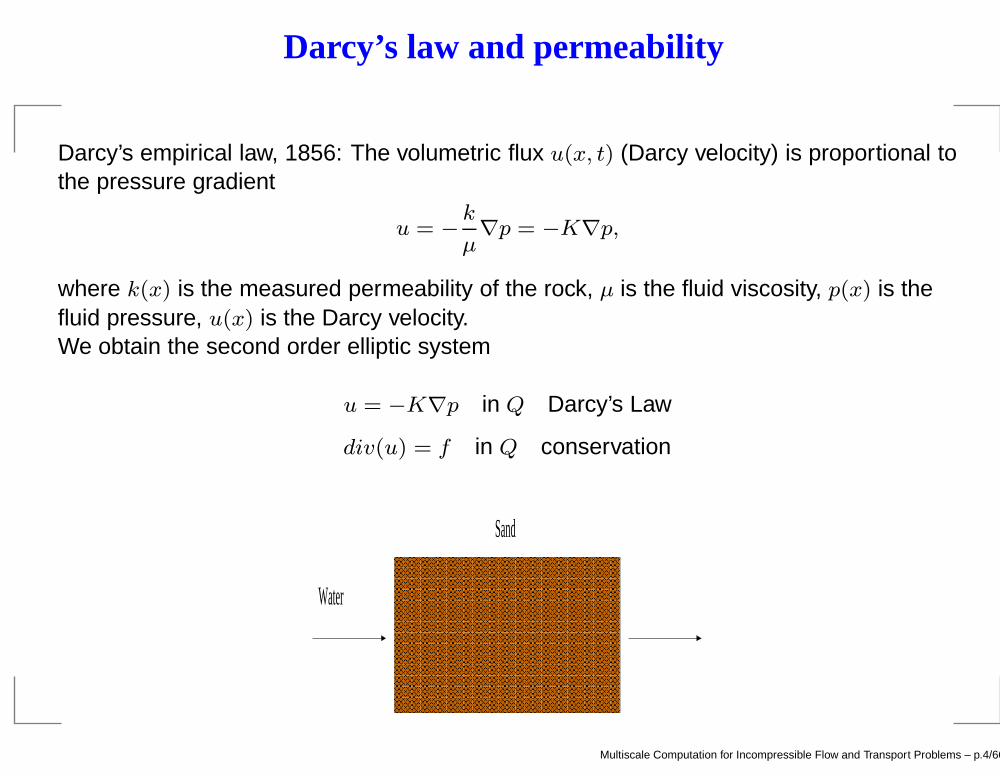
Darcy’s empirical law, 1856: The volumetric flux u(x, t) (Darcy velocity) is proportional tothe pressure gradient
u = −k
µ∇p = −K∇p,
where k(x) is the measured permeability of the rock, µ is the fluid viscosity, p(x) is thefluid pressure, u(x) is the Darcy velocity.We obtain the second order elliptic system
Multiscale Computation for Incompressible Flow and Transport Problems – p.6/66
Multiscale Finite Element Methods
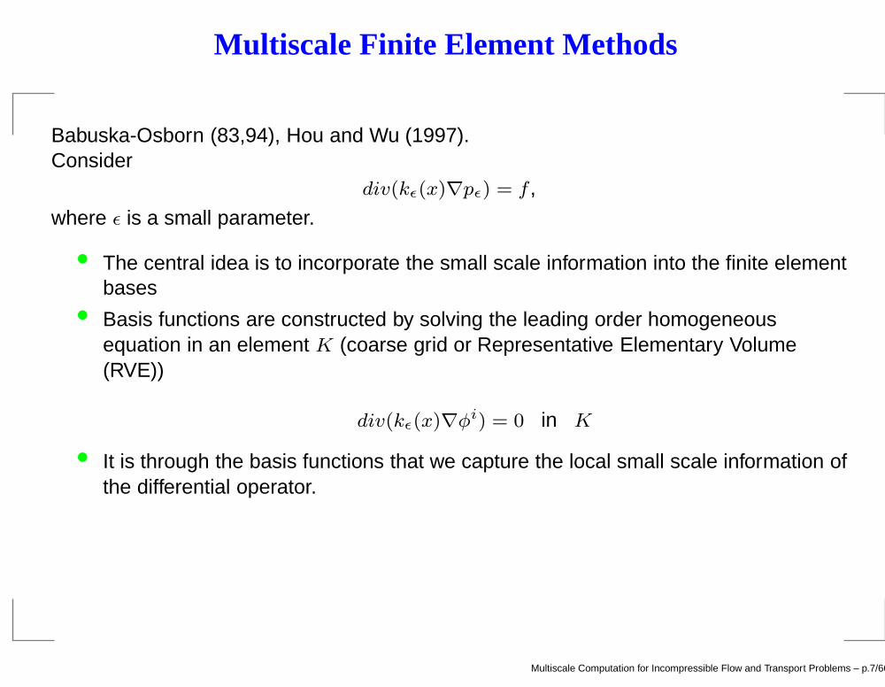
Babuska-Osborn (83,94), Hou and Wu (1997).Consider
div(kǫ(x)∇pǫ) = f ,
where ǫ is a small parameter.
• The central idea is to incorporate the small scale information into the finite elementbases
• Basis functions are constructed by solving the leading order homogeneousequation in an element K (coarse grid or Representative Elementary Volume(RVE))
div(kǫ(x)∇φi) = 0 in K
• It is through the basis functions that we capture the local small scale information ofthe differential operator.
Multiscale Computation for Incompressible Flow and Transport Problems – p.7/66
Multiscale Finite Element Methods
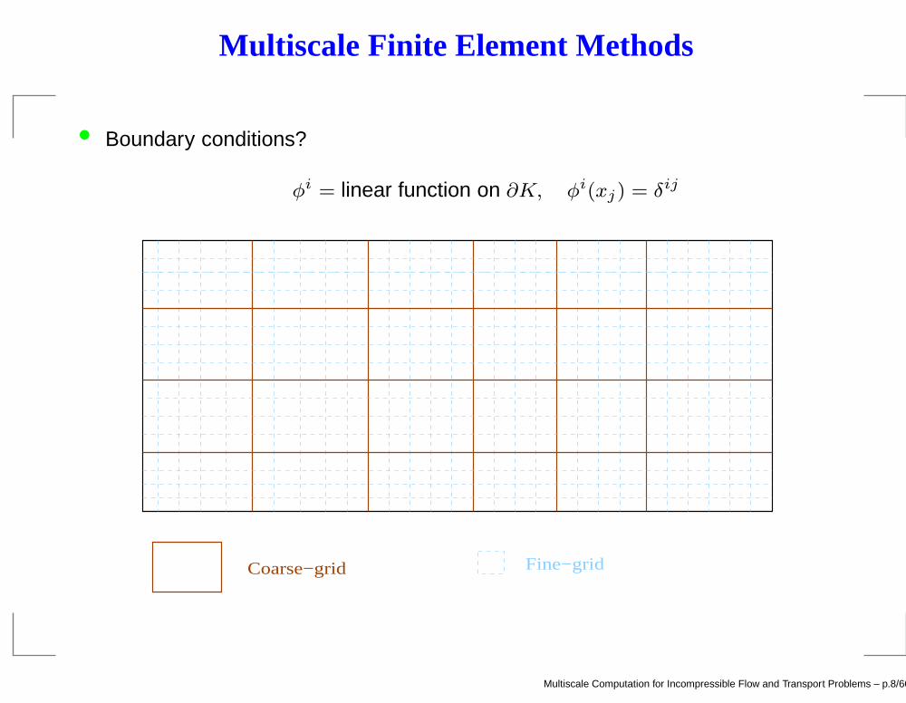
• Boundary conditions?
φi = linear function on ∂K, φi(xj) = δij
Coarse−grid Fine−grid
Multiscale Computation for Incompressible Flow and Transport Problems – p.8/66
Basis functions
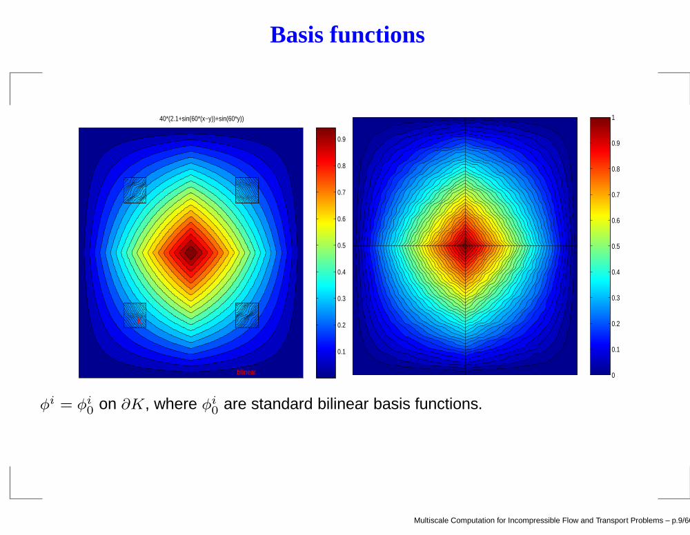
40*(2.1+sin(60*(x−y))+sin(60*y))
0.1
0.2
0.3
0.4
0.5
0.6
0.7
0.8
0.9
K
bilinear 0
0.1
0.2
0.3
0.4
0.5
0.6
0.7
0.8
0.9
1
φi = φi0 on ∂K, where φi
0 are standard bilinear basis functions.
Multiscale Computation for Incompressible Flow and Transport Problems – p.9/66
Multiscale Finite Element Methods
• Except for the multiscale basis functions, MsFEM is the same as the traditionalFEM (finite element method). Find ph
ǫ ∈ V h = {φi} such that
k(phǫ , v
h) = f(vh) ∀vh ∈ V h,
where
k(u, v) =
Z
Qkǫ
ij(x)∂u
∂xi
∂v
∂xjdx, f(v) =
Z
Qfvdx
• The coupling of the small scales is through the variational formulation
• Solution has the form pǫ ≈ p0(x) + ǫNk(x/ǫ) ∂∂xk
p0(x), if k(x/ǫ) is periodic.
• If standard finite element method is used (linear basis functions):
‖pǫ − phǫ ‖H1(Q) ≤ Chα‖pǫ‖H1+α(Q) = O(
hα
ǫα).
Thus, h≪ ǫ, which is not affordable in practice.
Multiscale Computation for Incompressible Flow and Transport Problems – p.10/66
Relation to other approaches
Subgrid modeling (by I. Babuska, T. Hughes, G. Allaire, T. Arbogast, and others)Subgrid stabilization (by F. Brezzi, L Franco, J.L. Guermond, T. Hughes, A. Russo, andothers).
• Multiscale finite element methods (Hou and Wu, Allaire and Brizzi, ...)• Multiscale finite volume methods (Jenny, Lee and Tchelepi)
• Multiscale finite element methods based on two-scale convergence (C. Schwab,...)
• Variational multiscale method and residual free bubble methods (T. Hughes, F.Brezzi, T. Arbogast, G. Sangalli,...)
• Partition of Unity Methods (Babuska, Osborn, Fish, ...)
• Wavelet based homogenization (Dorobantu, Engquist,...)
• Heterogeneous multiscale methods (E and Engquist ...)
Multiscale Computation for Incompressible Flow and Transport Problems – p.11/66
Convergence property of MsFEM
Consider kǫ(x) = k(x/ǫ), where k(y) is periodic in y.h - computational mesh size.Theorem Denote ph
ǫ the numerical solution obtained by MsFEM, and pǫ the solution of theoriginal problem. Then,If h >> ǫ,
‖pǫ − phǫ ‖1,Q ≤ C(h+
rǫ
h)
• This theorem shows that MsFEM converges to the correct solution as ǫ→ 0
• The ratio ǫ/h reflects two intrinsic scales. We call ǫ/h the resonance error
• The theorem shows that there is a scale resonance when h ≈ ǫ. Numericalexperiments confirm the scale resonance.
Multiscale Computation for Incompressible Flow and Transport Problems – p.12/66
Resonance errors
• For problems with scale separation, we can choose h≫ ǫ in order to avoid theresonance, but for problems with continuous spectrum of scales, we cannot avoidthis resonance.
• To demonstrate the influence of the boundary condition of the basis function onthe overall accuracy of the method we perform multiscale expansion of φi
• Multiscale expansion of φi
φi = φ0(x) + ǫφ1(x, x/ǫ) + ǫθǫ + . . . ,
• φ1(x, x/ǫ) = Nk(x/ǫ) ∂∂xk
φ0, where Nk(x/ǫ) is a periodic function which depends
on k(x/ǫ).
• θǫ satisfies
div(kǫ∇θǫ) = 0 in K, θiǫ = −φ1(x, x/ǫ) + (φi − φ0)/ǫ on ∂K
• Oscillations near the boundaries (in ǫ vicinity) of θiǫ lead to the resonance error
Multiscale Computation for Incompressible Flow and Transport Problems – p.13/66
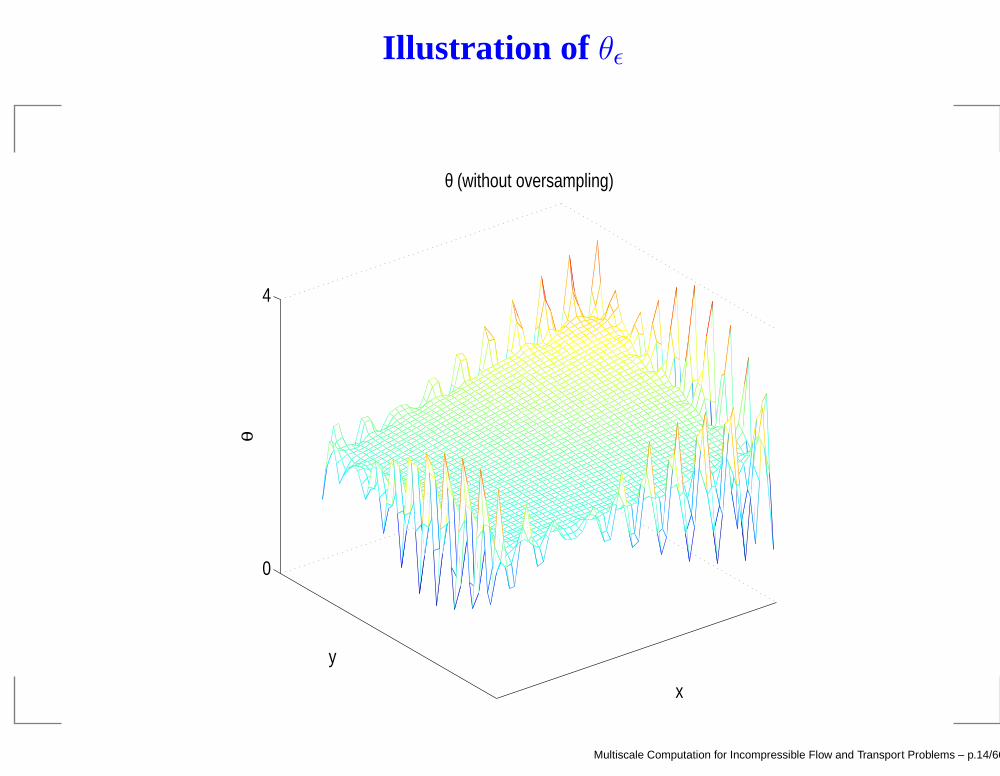
Illustration of θǫ
0
4
x
θ (without oversampling)
y
θ
Multiscale Computation for Incompressible Flow and Transport Problems – p.14/66
Oversampling technique
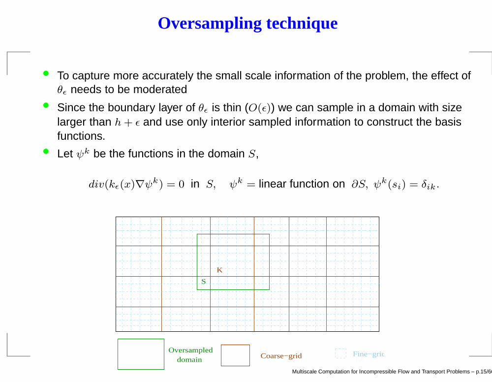
• To capture more accurately the small scale information of the problem, the effect ofθǫ needs to be moderated
• Since the boundary layer of θǫ is thin (O(ǫ)) we can sample in a domain with sizelarger than h+ ǫ and use only interior sampled information to construct the basisfunctions.
• Let ψk be the functions in the domain S,
div(kǫ(x)∇ψk) = 0 in S, ψk = linear function on ∂S, ψk(si) = δik.
Fine−gridCoarse−gridOversampled domain
S
K
Multiscale Computation for Incompressible Flow and Transport Problems – p.15/66
Oversampling technique
• The base functions in a domain K ⊂ S constructed as
φi|K =X
cijψj |K , φi(xk) = δik
• The method is non-conforming.
• The derivation of the convergence rate uses the homogenization methodcombined with the techniques of non-conforming finite element method (Efendievet al., SIAM Num. Anal. 1999)
• By a correct choice of the boundary condition of the basis functions we can reducethe effects of the boundary layer in θ.
Multiscale Computation for Incompressible Flow and Transport Problems – p.16/66
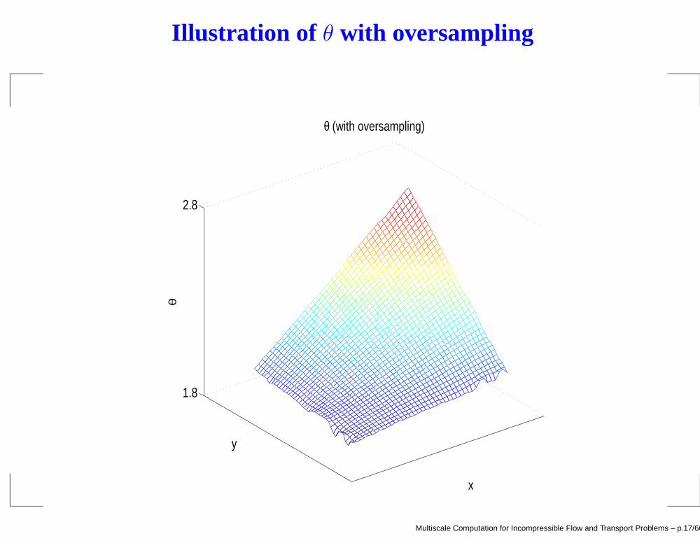
Illustration of θ with oversampling
1.8
2.8
x
θ (with oversampling)
y
θ
Multiscale Computation for Incompressible Flow and Transport Problems – p.17/66
Multiscale Computation for Incompressible Flow and Transport Problems – p.18/66
MsFEM for problems with scale separation
For periodic problems or problems with scale separation, multiscale finite elementmethods can take an advantage of scale separation. Local problems can be solved inRVE
div(k∇φi) = 0
φi = φi0 on ∂ RV E.
Basis functions can be also approximated
φi = φi0 +Nǫ · ∇φi
0,
where φ0i is linear basis functions and N is the periodic solution of auxiliary problem in
ǫ-size period−div(kǫ(x)(∇N + I)) = 0.
(cf. Durlofsky 1981, etc.).Note, the above procedure works when “homogenization by periodization” is applicable(e.g., random homogeneous case).
Multiscale Computation for Incompressible Flow and Transport Problems – p.19/66
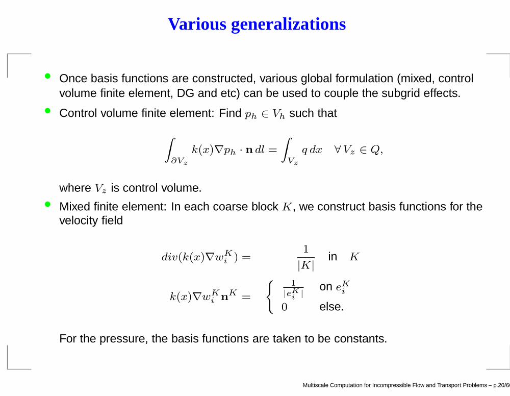
Various generalizations
• Once basis functions are constructed, various global formulation (mixed, controlvolume finite element, DG and etc) can be used to couple the subgrid effects.
• Control volume finite element: Find ph ∈ Vh such that
Z
∂Vz
k(x)∇ph · n dl =
Z
Vz
q dx ∀Vz ∈ Q,
where Vz is control volume.• Mixed finite element: In each coarse block K, we construct basis functions for the
velocity field
div(k(x)∇wKi ) =
1
|K|in K
k(x)∇wKi n
K =
(1
|eKi
|on eK
i
0 else.
For the pressure, the basis functions are taken to be constants.
Multiscale Computation for Incompressible Flow and Transport Problems – p.20/66
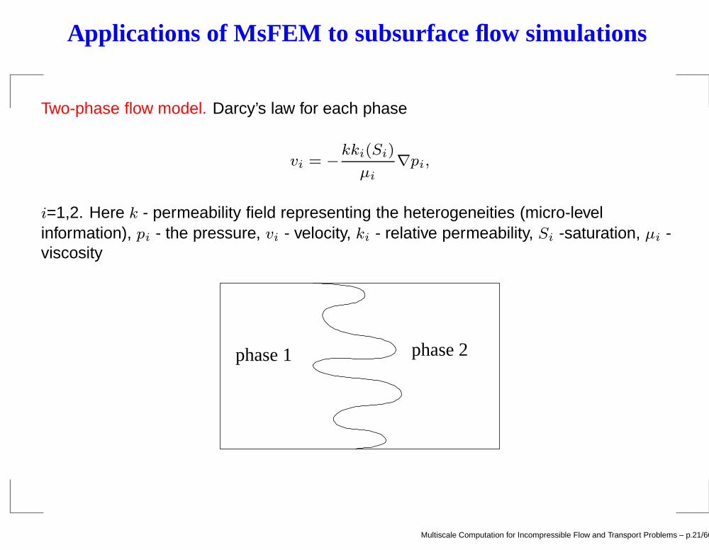
Applications of MsFEM to subsurface flow simulations
Two-phase flow model. Darcy’s law for each phase
vi = −kki(Si)
µi∇pi,
i=1,2. Here k - permeability field representing the heterogeneities (micro-levelinformation), pi - the pressure, vi - velocity, ki - relative permeability, Si -saturation, µi -viscosity
phase 1 phase 2
Multiscale Computation for Incompressible Flow and Transport Problems – p.21/66
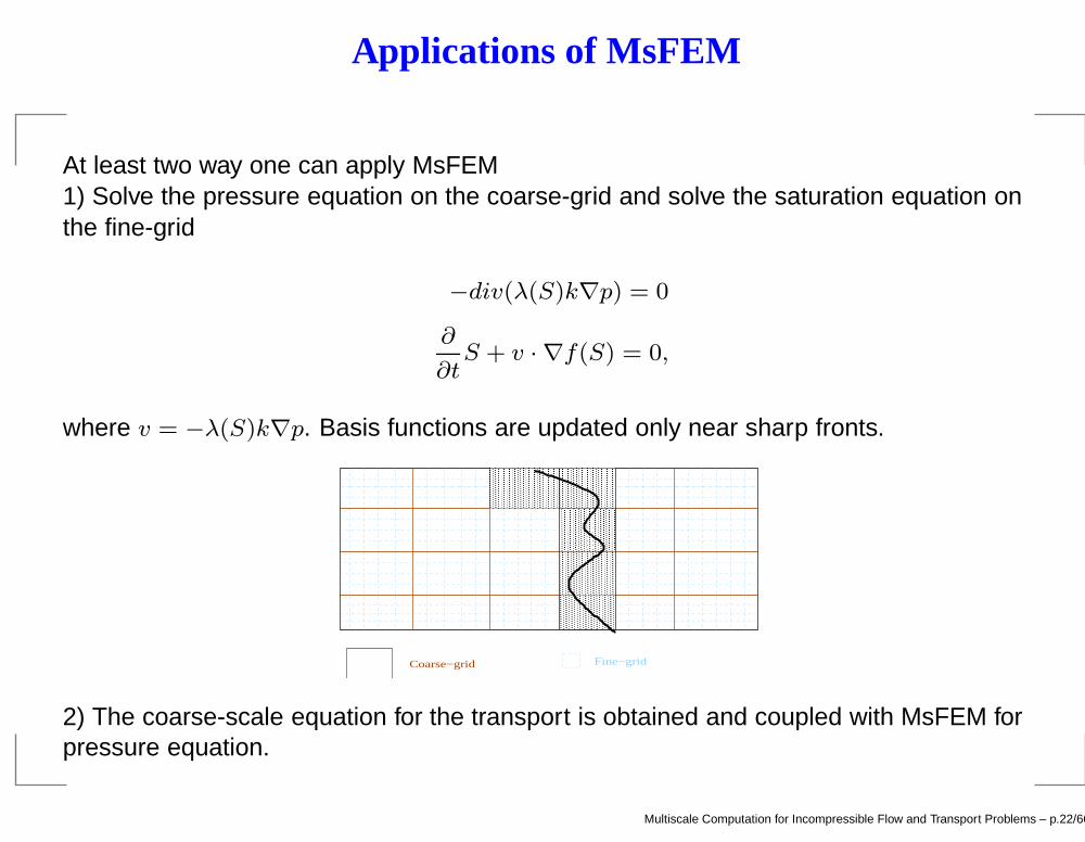
Applications of MsFEM
At least two way one can apply MsFEM1) Solve the pressure equation on the coarse-grid and solve the saturation equation onthe fine-grid
−div(λ(S)k∇p) = 0
∂
∂tS + v · ∇f(S) = 0,
where v = −λ(S)k∇p. Basis functions are updated only near sharp fronts.
2) The coarse-scale equation for the transport is obtained and coupled with MsFEM forpressure equation.
Multiscale Computation for Incompressible Flow and Transport Problems – p.22/66
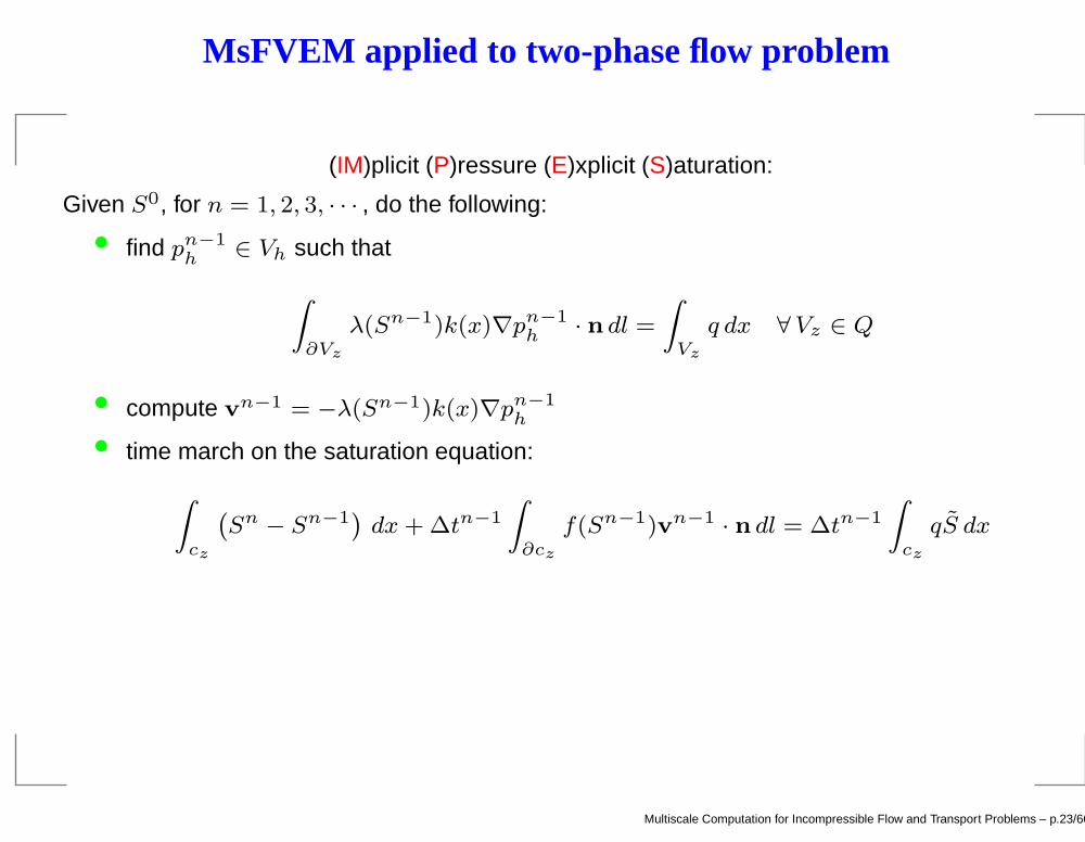
MsFVEM applied to two-phase flow problem
(IM)plicit (P)ressure (E)xplicit (S)aturation:
Given S0, for n = 1, 2, 3, · · · , do the following:
• find pn−1h ∈ Vh such that
Z
∂Vz
λ(Sn−1)k(x)∇pn−1h · n dl =
Z
Vz
q dx ∀Vz ∈ Q
• compute vn−1 = −λ(Sn−1)k(x)∇pn−1h
• time march on the saturation equation:
Z
cz
`Sn − Sn−1
´dx+ ∆tn−1
Z
∂cz
f(Sn−1)vn−1 · n dl = ∆tn−1
Z
cz
qS dx
Multiscale Computation for Incompressible Flow and Transport Problems – p.23/66
Numerical Setting
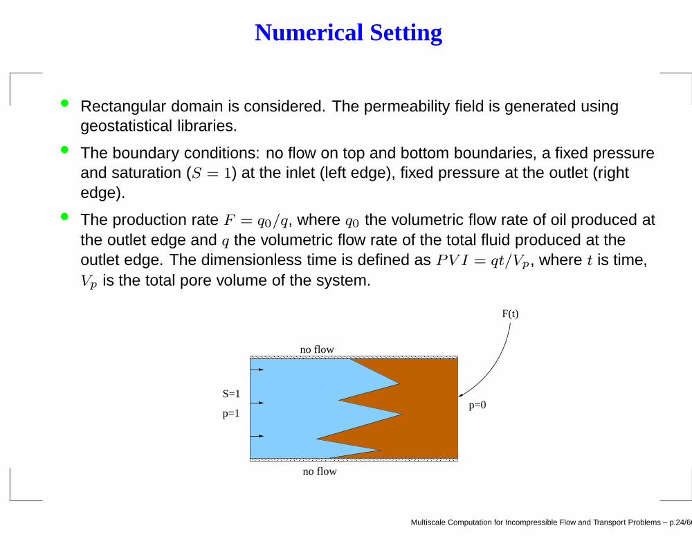
• Rectangular domain is considered. The permeability field is generated usinggeostatistical libraries.
• The boundary conditions: no flow on top and bottom boundaries, a fixed pressureand saturation (S = 1) at the inlet (left edge), fixed pressure at the outlet (rightedge).
• The production rate F = q0/q, where q0 the volumetric flow rate of oil produced atthe outlet edge and q the volumetric flow rate of the total fluid produced at theoutlet edge. The dimensionless time is defined as PV I = qt/Vp, where t is time,Vp is the total pore volume of the system.
������������������������������������������������
������������������������������������������������
no flow
no flow
S=1
p=1p=0
F(t)
Multiscale Computation for Incompressible Flow and Transport Problems – p.24/66
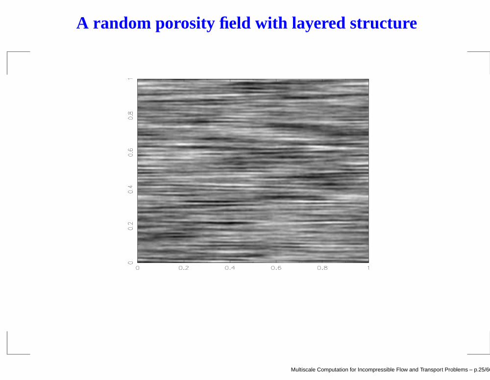
A random porosity field with layered structure
Multiscale Computation for Incompressible Flow and Transport Problems – p.25/66
Recovery of fine scale velocity
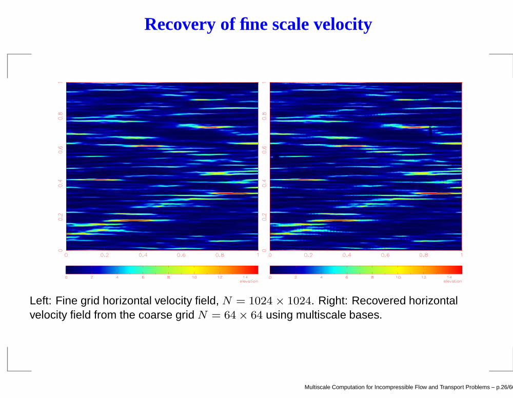
Left: Fine grid horizontal velocity field, N = 1024 × 1024. Right: Recovered horizontalvelocity field from the coarse grid N = 64 × 64 using multiscale bases.
Multiscale Computation for Incompressible Flow and Transport Problems – p.26/66
Recovery of fine scale saturation
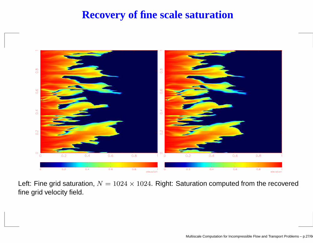
Left: Fine grid saturation, N = 1024 × 1024. Right: Saturation computed from the recoveredfine grid velocity field.
Multiscale Computation for Incompressible Flow and Transport Problems – p.27/66
Fractional flow and total flow curves
0 0.5 1 1.5 20
0.1
0.2
0.3
0.4
0.5
0.6
0.7
0.8
0.9
1
PVI
F
finemodified MsFVMstandard MsFVM
0 0.5 1 1.5 2
3
4
5
6
7
8
9
10
11
PVI
Q
finemodified MsFVMstandard MsFVM
Fractional flow and total flow for a realization of permeability field with exponential variogramand lx = 0.4, lz = 0.02, σ = 1.5.
Multiscale Computation for Incompressible Flow and Transport Problems – p.28/66
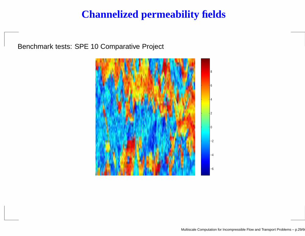
Channelized permeability fields
Benchmark tests: SPE 10 Comparative Project
−6
−4
−2
0
2
4
6
8
Multiscale Computation for Incompressible Flow and Transport Problems – p.29/66
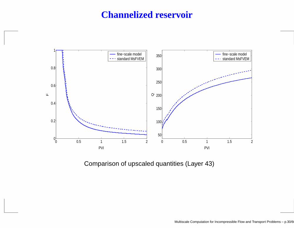
Channelized reservoir
0 0.5 1 1.5 20
0.2
0.4
0.6
0.8
1
PVI
F
fine−scale modelstandard MsFVEM
0 0.5 1 1.5 2
50
100
150
200
250
300
350
PVIQ
fine−scale modelstandard MsFVEM
Comparison of upscaled quantities (Layer 43)
Multiscale Computation for Incompressible Flow and Transport Problems – p.30/66
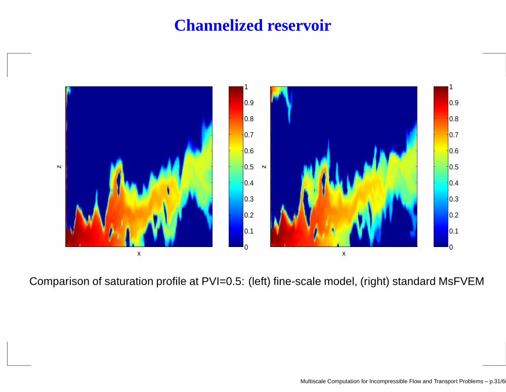
Channelized reservoir
x
z
0
0.1
0.2
0.3
0.4
0.5
0.6
0.7
0.8
0.9
1
xz
0
0.1
0.2
0.3
0.4
0.5
0.6
0.7
0.8
0.9
1
Comparison of saturation profile at PVI=0.5: (left) fine-scale model, (right) standard MsFVEM
Multiscale Computation for Incompressible Flow and Transport Problems – p.31/66
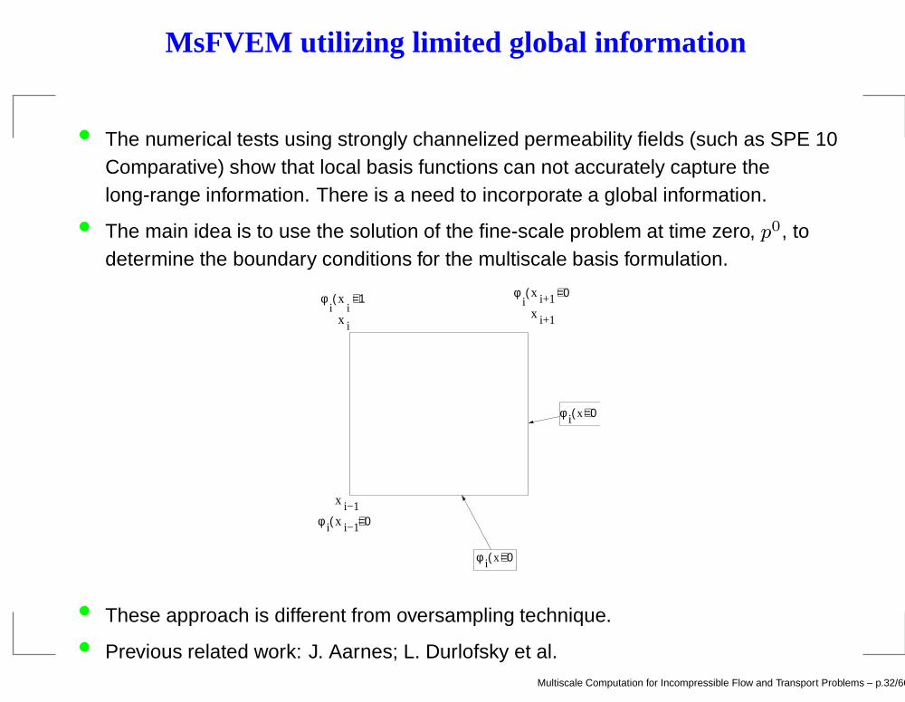
MsFVEM utilizing limited global information
• The numerical tests using strongly channelized permeability fields (such as SPE 10Comparative) show that local basis functions can not accurately capture thelong-range information. There is a need to incorporate a global information.
• The main idea is to use the solution of the fine-scale problem at time zero, p0, todetermine the boundary conditions for the multiscale basis formulation.
x
x
xi
i−1
i+1
x i−1
i+1xxi
φ (
φ (
φ ()=1 )=0
)=0
i
i
i
φ ( )=0
φ ( )=0
i
x
x
i
• These approach is different from oversampling technique.
• Previous related work: J. Aarnes; L. Durlofsky et al.Multiscale Computation for Incompressible Flow and Transport Problems – p.32/66
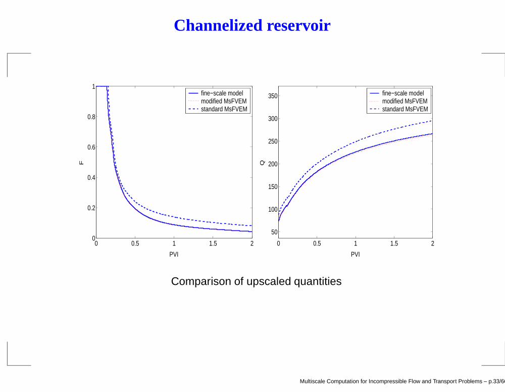
Channelized reservoir
0 0.5 1 1.5 20
0.2
0.4
0.6
0.8
1
PVI
F
fine−scale modelmodified MsFVEMstandard MsFVEM
0 0.5 1 1.5 2
50
100
150
200
250
300
350
PVIQ
fine−scale modelmodified MsFVEMstandard MsFVEM
Comparison of upscaled quantities
Multiscale Computation for Incompressible Flow and Transport Problems – p.33/66
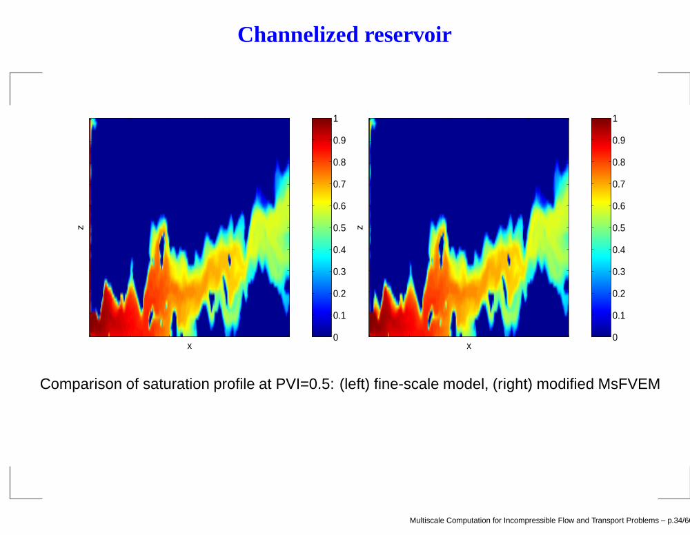
Channelized reservoir
x
z
0
0.1
0.2
0.3
0.4
0.5
0.6
0.7
0.8
0.9
1
xz
0
0.1
0.2
0.3
0.4
0.5
0.6
0.7
0.8
0.9
1
Comparison of saturation profile at PVI=0.5: (left) fine-scale model, (right) modified MsFVEM
Multiscale Computation for Incompressible Flow and Transport Problems – p.34/66
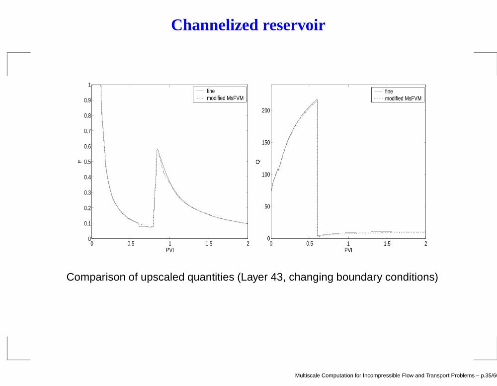
Channelized reservoir
0 0.5 1 1.5 20
0.1
0.2
0.3
0.4
0.5
0.6
0.7
0.8
0.9
1
PVI
F
finemodified MsFVM
0 0.5 1 1.5 20
50
100
150
200
PVIQ
finemodified MsFVM
Comparison of upscaled quantities (Layer 43, changing boundary conditions)
Multiscale Computation for Incompressible Flow and Transport Problems – p.35/66
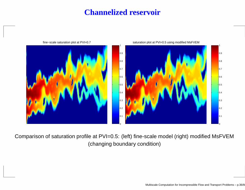
Channelized reservoir
fine−scale saturation plot at PVI=0.7
0
0.1
0.2
0.3
0.4
0.5
0.6
0.7
0.8
0.9
1saturation plot at PVI=0.5 using modified MsFVEM
0
0.1
0.2
0.3
0.4
0.5
0.6
0.7
0.8
0.9
1
Comparison of saturation profile at PVI=0.5: (left) fine-scale model (right) modified MsFVEM(changing boundary condition)
Multiscale Computation for Incompressible Flow and Transport Problems – p.36/66
Brief Analysis
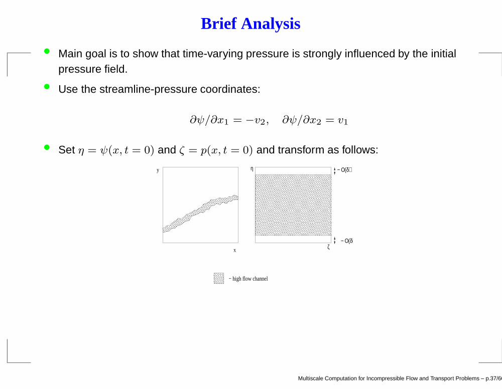
• Main goal is to show that time-varying pressure is strongly influenced by the initialpressure field.
• Use the streamline-pressure coordinates:
∂ψ/∂x1 = −v2, ∂ψ/∂x2 = v1
• Set η = ψ(x, t = 0) and ζ = p(x, t = 0) and transform as follows:
Multiscale Computation for Incompressible Flow and Transport Problems – p.39/66
Extensions
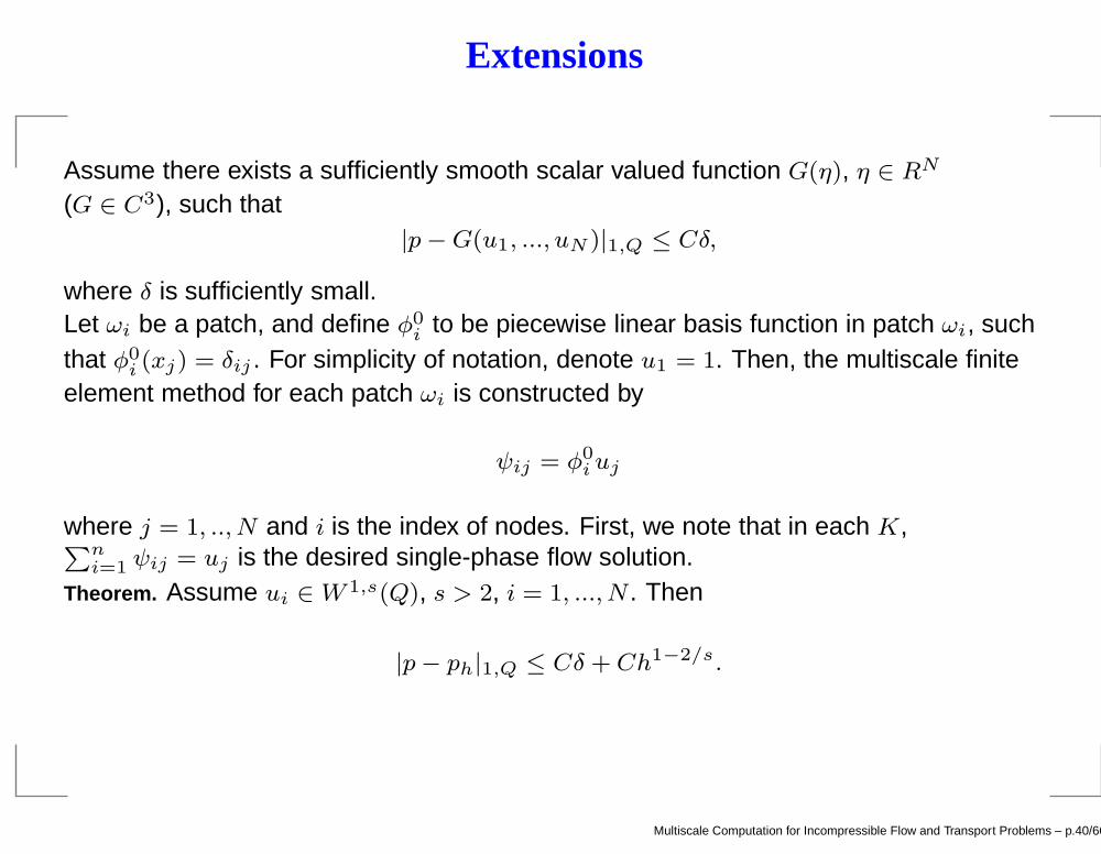
Assume there exists a sufficiently smooth scalar valued function G(η), η ∈ RN
(G ∈ C3), such that|p−G(u1, ..., uN )|1,Q ≤ Cδ,
where δ is sufficiently small.Let ωi be a patch, and define φ0
i to be piecewise linear basis function in patch ωi, suchthat φ0
i (xj) = δij . For simplicity of notation, denote u1 = 1. Then, the multiscale finiteelement method for each patch ωi is constructed by
ψij = φ0i uj
where j = 1, ..,N and i is the index of nodes. First, we note that in each K,Pni=1 ψij = uj is the desired single-phase flow solution.
Theorem. Assume ui ∈W 1,s(Q), s > 2, i = 1, ...,N . Then
|p− ph|1,Q ≤ Cδ + Ch1−2/s.
Multiscale Computation for Incompressible Flow and Transport Problems – p.40/66
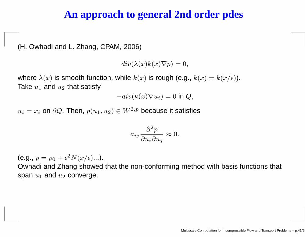
An approach to general 2nd order pdes
(H. Owhadi and L. Zhang, CPAM, 2006)
div(λ(x)k(x)∇p) = 0,
where λ(x) is smooth function, while k(x) is rough (e.g., k(x) = k(x/ǫ)).Take u1 and u2 that satisfy
−div(k(x)∇ui) = 0 in Q,
ui = xi on ∂Q. Then, p(u1, u2) ∈W 2,p because it satisfies
aij∂2p
∂ui∂uj≈ 0.
(e.g., p = p0 + ǫ2N(x/ǫ)...).Owhadi and Zhang showed that the non-conforming method with basis functions thatspan u1 and u2 converge.
Multiscale Computation for Incompressible Flow and Transport Problems – p.41/66
Two-phase flow equations in flow-based coor.
∂
∂ψ
„k2λ(S)
∂P
∂ψ
«+
∂
∂p
„λ(S)
∂P
∂p
«= 0.
∂S
∂t+ (v · ∇ψ)
∂f(S)
∂ψ+ (v · ∇p)
∂f(S)
∂p= 0.
Consider λ(S) = 1. Homogenization of hyperbolic equations.
Sǫt + vǫ
0f(Sǫ)p = 0
S(p, ψ, t = 0) = S0,
vǫ0(p) = v0(p,
p
ǫ).
Multiscale Computation for Incompressible Flow and Transport Problems – p.42/66
Homogenization of transport
Then, for each ψ, it can be shown that Sǫ(p, ψ, t) → S(p, ψ, t) in L1((0, 1) × (0, T )),where S satisfies
St + v0f(S)p = 0,
where v0 is harmonic average of vǫ0, i.e.,
1
vǫ0
→1
v0weak ∗ in L∞(0, 1).
Theorem.
‖Sǫ − S‖n ≤ Gǫ1/n.
Note. S can be considered as an upscaled Sǫ along streamlines. Can we averageacross streamlines?
Multiscale Computation for Incompressible Flow and Transport Problems – p.43/66
Numerical results
−3
−2
−1
0
1
2
3
−1
0
1
2
3
4
5
6
7
8
9
−4
−2
0
2
4
6
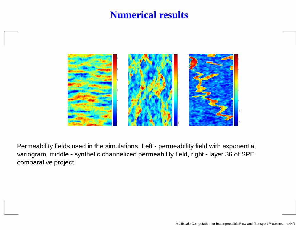
8
Permeability fields used in the simulations. Left - permeability field with exponentialvariogram, middle - synthetic channelized permeability field, right - layer 36 of SPEcomparative project
Multiscale Computation for Incompressible Flow and Transport Problems – p.44/66
Numerical results
0.1
0.2
0.3
0.4
0.5
0.6
0.7
0.8
0.9
0.1
0.2
0.3
0.4
0.5
0.6
0.7
0.8
0.9
0.1
0.2
0.3
0.4
0.5
0.6
0.7
0.8
0.9
0.1
0.2
0.3
0.4
0.5
0.6
0.7
0.8
0.9
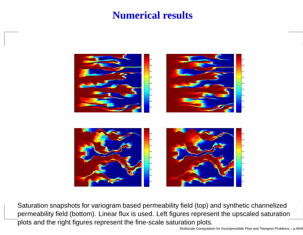
Saturation snapshots for variogram based permeability field (top) and synthetic channelizedpermeability field (bottom). Linear flux is used. Left figures represent the upscaled saturationplots and the right figures represent the fine-scale saturation plots.
Multiscale Computation for Incompressible Flow and Transport Problems – p.45/66
Numerical results
0.1
0.2
0.3
0.4
0.5
0.6
0.7
0.8
0.9
0.1
0.2
0.3
0.4
0.5
0.6
0.7
0.8
0.9
0.1
0.2
0.3
0.4
0.5
0.6
0.7
0.8
0.9
0.1
0.2
0.3
0.4
0.5
0.6
0.7
0.8
0.9
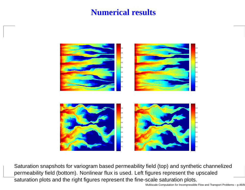
Saturation snapshots for variogram based permeability field (top) and synthetic channelizedpermeability field (bottom). Nonlinear flux is used. Left figures represent the upscaledsaturation plots and the right figures represent the fine-scale saturation plots.
Multiscale Computation for Incompressible Flow and Transport Problems – p.46/66
Numerical results
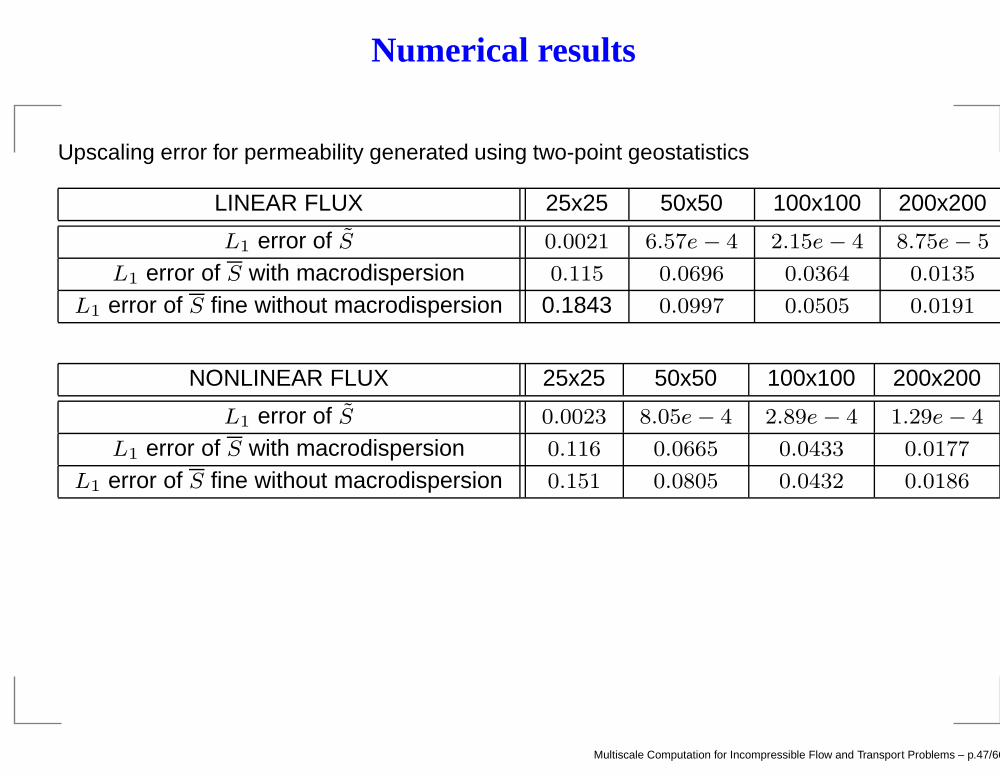
Upscaling error for permeability generated using two-point geostatistics
LINEAR FLUX 25x25 50x50 100x100 200x200
L1 error of S 0.0021 6.57e− 4 2.15e− 4 8.75e− 5
L1 error of S with macrodispersion 0.115 0.0696 0.0364 0.0135
L1 error of S fine without macrodispersion 0.1843 0.0997 0.0505 0.0191
NONLINEAR FLUX 25x25 50x50 100x100 200x200
L1 error of S 0.0023 8.05e− 4 2.89e− 4 1.29e− 4
L1 error of S with macrodispersion 0.116 0.0665 0.0433 0.0177
L1 error of S fine without macrodispersion 0.151 0.0805 0.0432 0.0186
Multiscale Computation for Incompressible Flow and Transport Problems – p.47/66
Numerical results
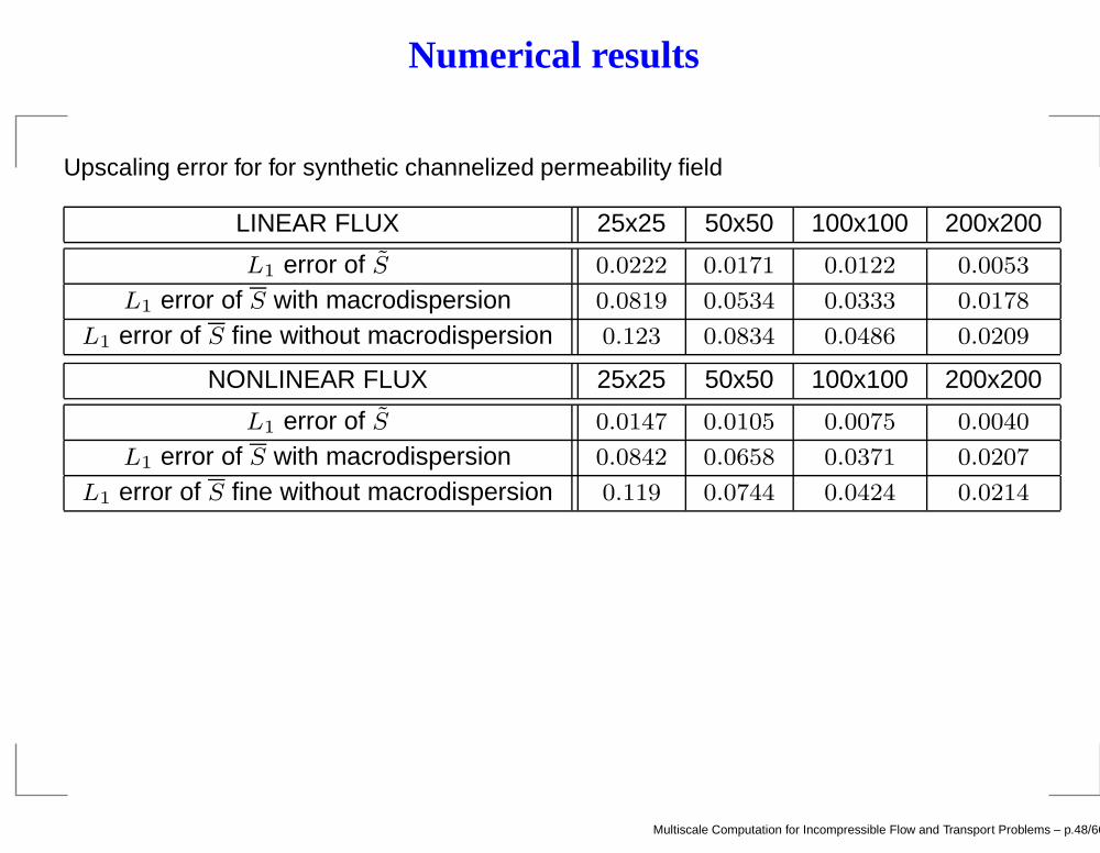
Upscaling error for for synthetic channelized permeability field
LINEAR FLUX 25x25 50x50 100x100 200x200
L1 error of S 0.0222 0.0171 0.0122 0.0053
L1 error of S with macrodispersion 0.0819 0.0534 0.0333 0.0178
L1 error of S fine without macrodispersion 0.123 0.0834 0.0486 0.0209
NONLINEAR FLUX 25x25 50x50 100x100 200x200
L1 error of S 0.0147 0.0105 0.0075 0.0040
L1 error of S with macrodispersion 0.0842 0.0658 0.0371 0.0207
L1 error of S fine without macrodispersion 0.119 0.0744 0.0424 0.0214
Multiscale Computation for Incompressible Flow and Transport Problems – p.48/66
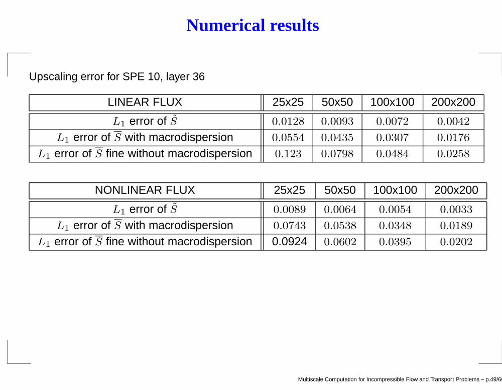
Numerical results
Upscaling error for SPE 10, layer 36
LINEAR FLUX 25x25 50x50 100x100 200x200
L1 error of S 0.0128 0.0093 0.0072 0.0042
L1 error of S with macrodispersion 0.0554 0.0435 0.0307 0.0176
L1 error of S fine without macrodispersion 0.123 0.0798 0.0484 0.0258
NONLINEAR FLUX 25x25 50x50 100x100 200x200
L1 error of S 0.0089 0.0064 0.0054 0.0033
L1 error of S with macrodispersion 0.0743 0.0538 0.0348 0.0189
L1 error of S fine without macrodispersion 0.0924 0.0602 0.0395 0.0202
Multiscale Computation for Incompressible Flow and Transport Problems – p.49/66
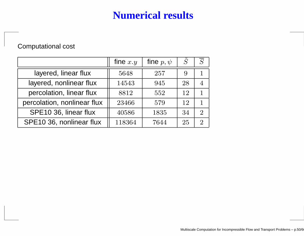
Numerical results
Computational cost
fine x.y fine p, ψ S S
layered, linear flux 5648 257 9 1
layered, nonlinear flux 14543 945 28 4
percolation, linear flux 8812 552 12 1
percolation, nonlinear flux 23466 579 12 1
SPE10 36, linear flux 40586 1835 34 2
SPE10 36, nonlinear flux 118364 7644 25 2
Multiscale Computation for Incompressible Flow and Transport Problems – p.50/66
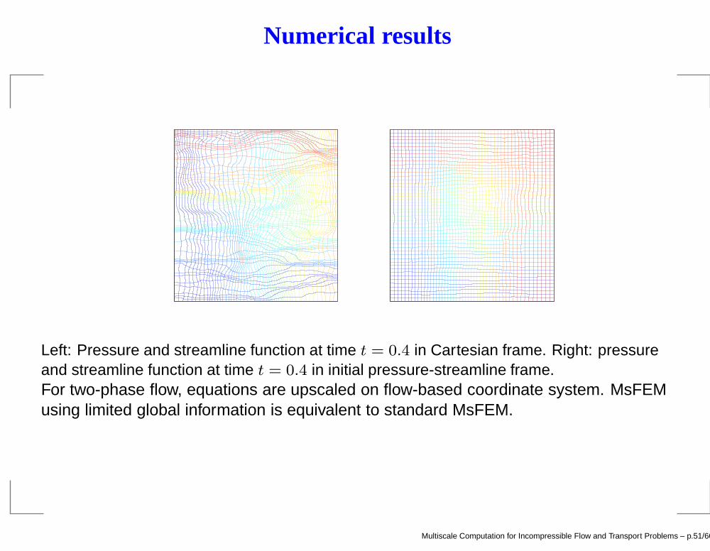
Numerical results
Left: Pressure and streamline function at time t = 0.4 in Cartesian frame. Right: pressureand streamline function at time t = 0.4 in initial pressure-streamline frame.For two-phase flow, equations are upscaled on flow-based coordinate system. MsFEMusing limited global information is equivalent to standard MsFEM.
Multiscale Computation for Incompressible Flow and Transport Problems – p.51/66
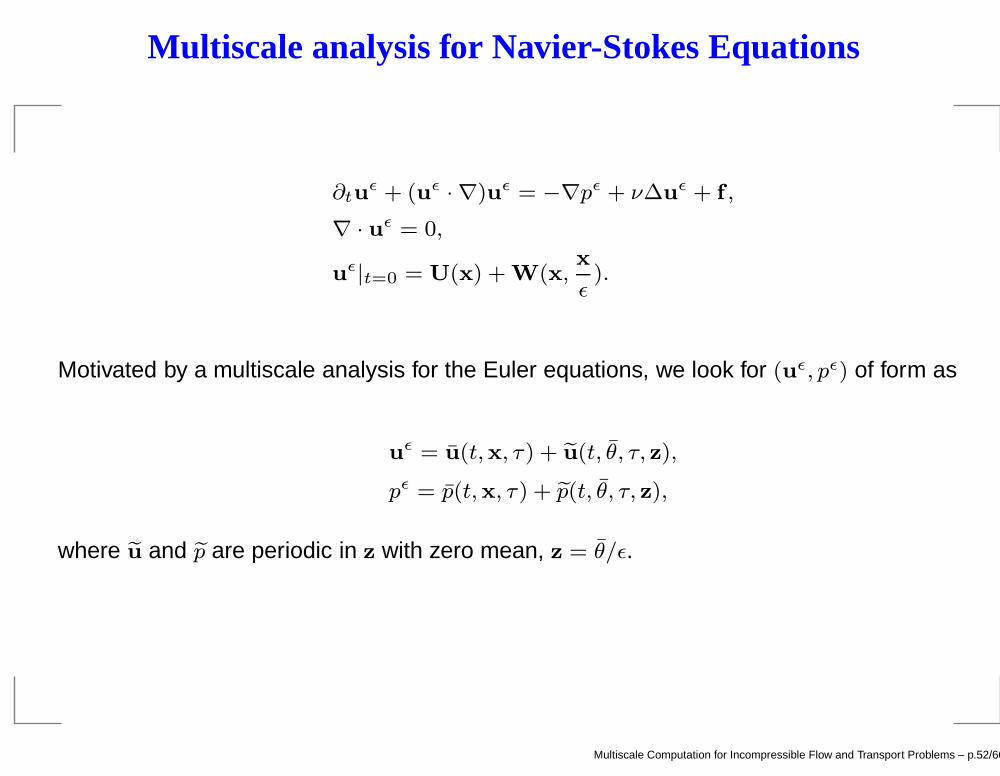
Multiscale analysis for Navier-Stokes Equations
∂tuǫ + (uǫ · ∇)uǫ = −∇pǫ + ν∆u
ǫ + f ,
∇ · uǫ = 0,
uǫ|t=0 = U(x) + W(x,
x
ǫ).
Motivated by a multiscale analysis for the Euler equations, we look for (uǫ, pǫ) of form as
uǫ = u(t,x, τ) + eu(t, θ, τ, z),
pǫ = p(t,x, τ) + ep(t, θ, τ, z),
where eu and ep are periodic in z with zero mean, z = θ/ǫ.
Multiscale Computation for Incompressible Flow and Transport Problems – p.52/66
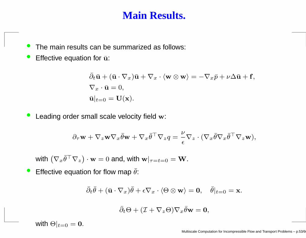
Main Results.
• The main results can be summarized as follows:• Effective equation for u:
∂tu + (u · ∇x)u + ∇x · 〈w ⊗ w〉 = −∇xp+ ν∆u + f ,
∇x · u = 0,
u|t=0 = U(x).
• Leading order small scale velocity field w:
∂τw + ∇zw∇xθw + ∇xθ⊤∇zq =
ν
ǫ∇z · (∇xθ∇xθ
⊤∇zw),
with`∇xθ⊤∇z
´· w = 0 and, with w|τ=t=0 = W.
• Effective equation for flow map θ:
∂tθ + (u · ∇x)θ + ǫ∇x · 〈Θ ⊗ w〉 = 0, θ|t=0 = x.
∂tΘ + (I + ∇zΘ)∇xθw = 0,
with Θ|t=0 = 0.Multiscale Computation for Incompressible Flow and Transport Problems – p.53/66
Numerical Experiments for 2D NSE
We use direct numerical simulation (DNS) to check the accuracy of our multiscaleanalysis. In computation, we choose ν = 10−4.
The DNS is performed using 512 by 512 mesh. The multiscale computations use 64 by64 on the coarse grid, and 32 by 32 for the subgrid.
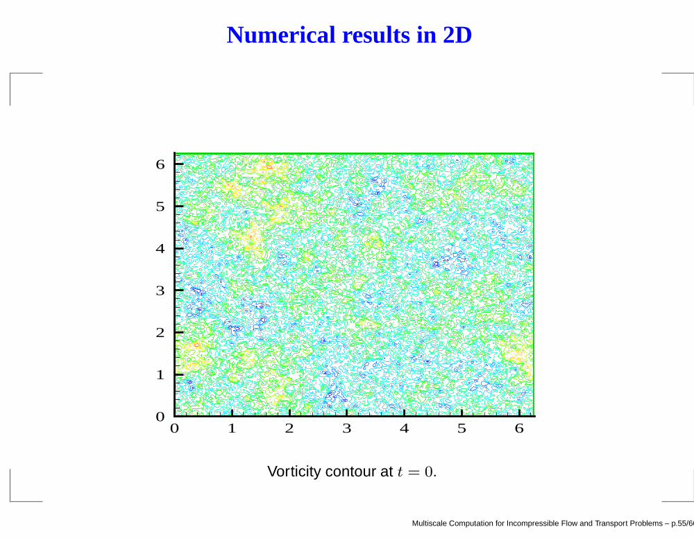
The initial vorticity is generated in Fourier space, satisfying bωk ≈ O(|k|−1) with randomphases.
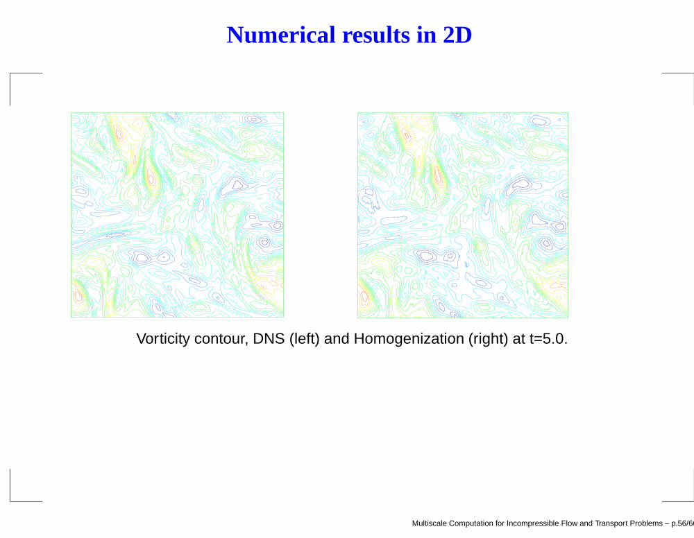
Our main objective is to test how accuate we can capture the inverse cascade of 2Dturbulence.
Multiscale Computation for Incompressible Flow and Transport Problems – p.54/66
Numerical results in 2D
0 1 2 3 4 5 60
1
2
3
4
5
6
Vorticity contour at t = 0.
Multiscale Computation for Incompressible Flow and Transport Problems – p.55/66
Numerical results in 2D
Vorticity contour, DNS (left) and Homogenization (right) at t=5.0.
Multiscale Computation for Incompressible Flow and Transport Problems – p.56/66
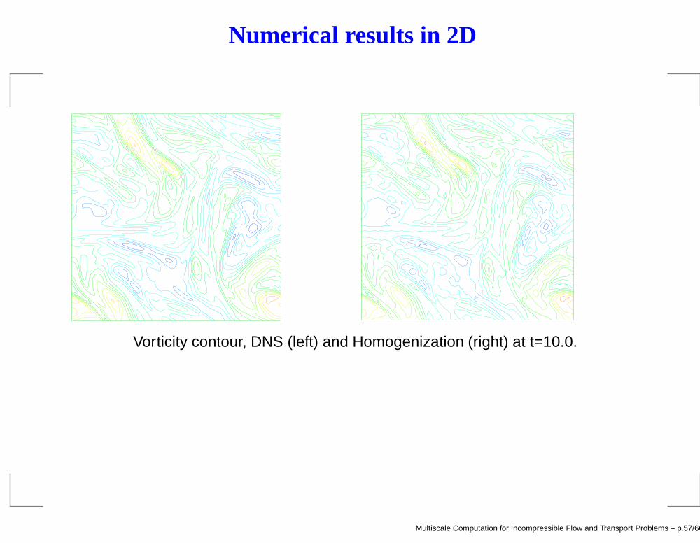
Numerical results in 2D
Vorticity contour, DNS (left) and Homogenization (right) at t=10.0.
Multiscale Computation for Incompressible Flow and Transport Problems – p.57/66
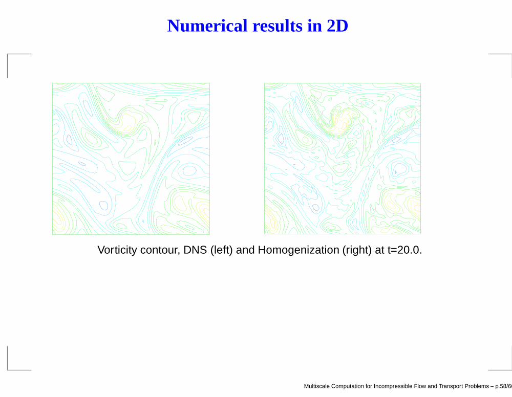
Numerical results in 2D
Vorticity contour, DNS (left) and Homogenization (right) at t=20.0.
Multiscale Computation for Incompressible Flow and Transport Problems – p.58/66
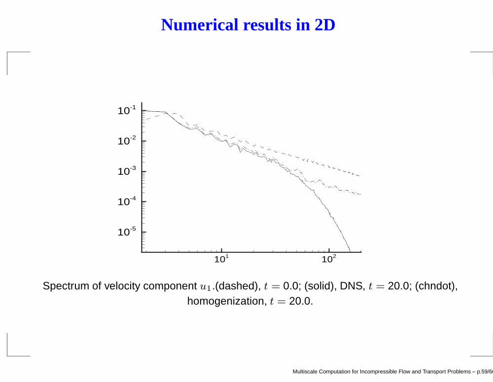
Numerical results in 2D
101 102
10-5
10-4
10-3
10-2
10-1
Spectrum of velocity component u1.(dashed), t = 0.0; (solid), DNS, t = 20.0; (chndot),homogenization, t = 20.0.
Multiscale Computation for Incompressible Flow and Transport Problems – p.59/66
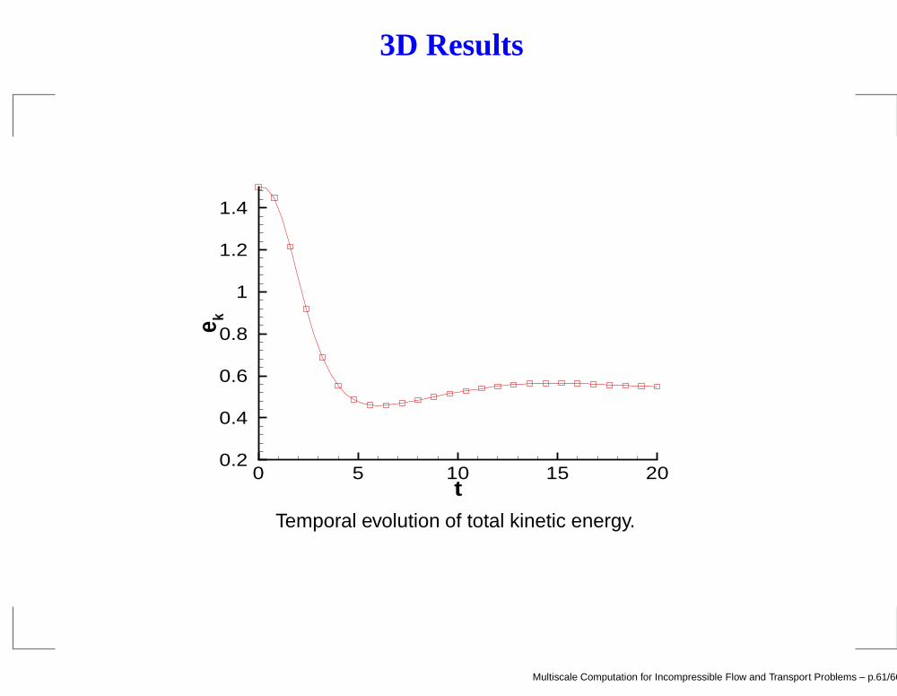
Numerical Experiments for 3D forced NSE
DNS is performed using 5123 mesh in a periodic box to check accuracy of the multiscalemethod.
The Taylor Reynolds number is 223 in our computation (equvilent viscosity is 0.0005).
The specific form of the forcing is given by
fk =δ
N
ukpuku
∗k
(-12)
N is the number of wave modes that are forced.
The above form of forcing ensures that the energy injection rate,Pf · u , is a constant
which is equal to δ. We chose δ = 0.1 for all of our runs.
Multiscale Computation for Incompressible Flow and Transport Problems – p.60/66
3D Results
t
e k
0 5 10 15 200.2
0.4
0.6
0.8
1
1.2
1.4
Temporal evolution of total kinetic energy.
Multiscale Computation for Incompressible Flow and Transport Problems – p.61/66
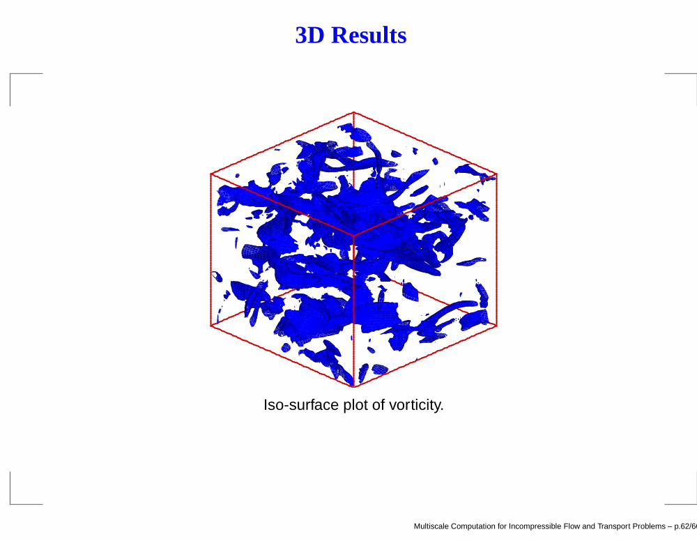
3D Results
Iso-surface plot of vorticity.
Multiscale Computation for Incompressible Flow and Transport Problems – p.62/66
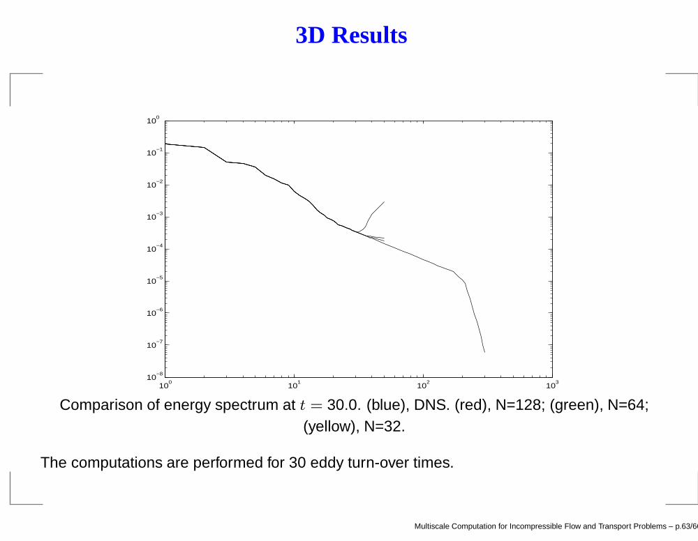
3D Results
100
101
102
103
10−8
10−7
10−6
10−5
10−4
10−3
10−2
10−1
100
Comparison of energy spectrum at t = 30.0. (blue), DNS. (red), N=128; (green), N=64;(yellow), N=32.
The computations are performed for 30 eddy turn-over times.
Multiscale Computation for Incompressible Flow and Transport Problems – p.63/66
3D Results
0 0.1 0.2 0.3 0.4 0.5 0.6 0.7 0.8 0.9 10
0.5
1
1.5
2
2.5
3
3.5
4
0 0.1 0.2 0.3 0.4 0.5 0.6 0.7 0.8 0.9 10.5
1
1.5
2
2.5
3
3.5
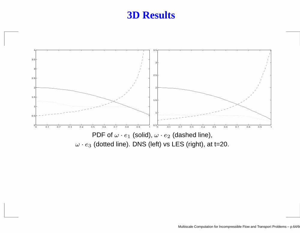
PDF of ω · e1 (solid), ω · e2 (dashed line),ω · e3 (dotted line). DNS (left) vs LES (right), at t=20.
Multiscale Computation for Incompressible Flow and Transport Problems – p.64/66
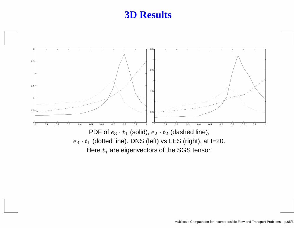
3D Results
0 0.1 0.2 0.3 0.4 0.5 0.6 0.7 0.8 0.9 10
0.5
1
1.5
2
2.5
3
0 0.1 0.2 0.3 0.4 0.5 0.6 0.7 0.8 0.9 10
0.5
1
1.5
2
2.5
3
3.5
PDF of e3 · t1 (solid), e2 · t2 (dashed line),e3 · t1 (dotted line). DNS (left) vs LES (right), at t=20.
Here tj are eigenvectors of the SGS tensor.
Multiscale Computation for Incompressible Flow and Transport Problems – p.65/66
Conclusions
• Multiscale finite element methods provide an effective multiscale computationalmethod for flow and transport in heterogeneous porous media.
• Resonance error can be effectively removed by the over-sampling technique.
• Long range scale interaction can be captured by incorporating limited globalinformation into the multiscale bases.
• Flow-based adaptive coordinates offer a natural physical coordinate to capture thelong range interaction in a channelized media.
• The hybrid Eulerian-Lagrangian coordinates offer a natural multiscale frame tocapture the nonlinear nonlocal scale interactions for the Navier-Stokes equations.
Multiscale Computation for Incompressible Flow and Transport Problems – p.66/66