65
MULTISCALE COMPUTATION: From Fast Solvers To Systematic Upscaling A. Brandt The Weizmann Institute of Science UCLA www.wisdom.weizmann.ac.il/ ~achi
| Date post: | 22-Dec-2015 |
| Category: |
Documents |
| View: | 213 times |
| Download: | 0 times |

MULTISCALE COMPUTATION:
From Fast SolversTo Systematic Upscaling
A. BrandtThe Weizmann Institute of ScienceUCLA
www.wisdom.weizmann.ac.il/~achi
Major scaling bottlenecks:computing
Elementary particles (QCD)
Schrödinger equationmoleculescondensed matter
Molecular dynamicsprotein folding, fluids, materials
Turbulence, weather, combustion,…
Inverse problemsda, control, medical imaging
Vision, recognition

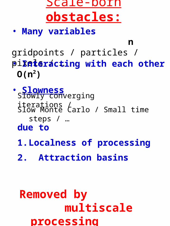
Scale-born obstacles:
• Many variables n gridpoints / particles / pixels / …
• Interacting with each other O(n2)
• Slowness
Slow Monte Carlo / Small time steps / …Slowly converging iterations /
due to
1. Localness of processing
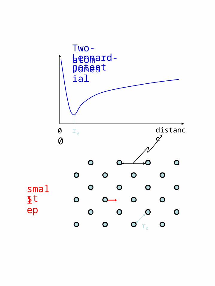
0
0r0 distance
Two-atomLennard-Jonespotential
r0
small step
small step
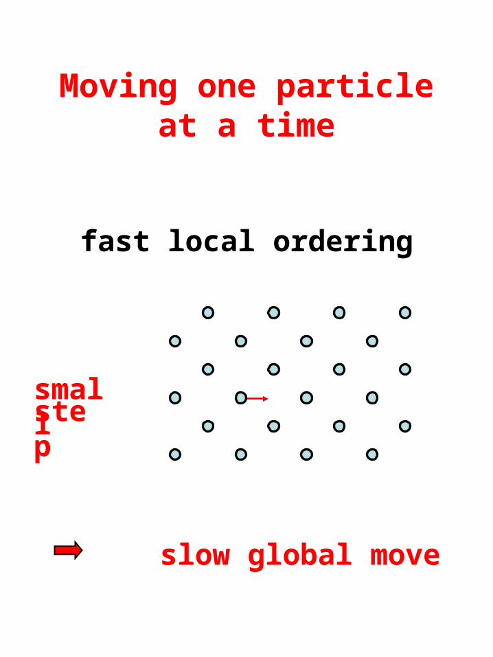
Moving one particle at a time
fast local ordering
slow global move

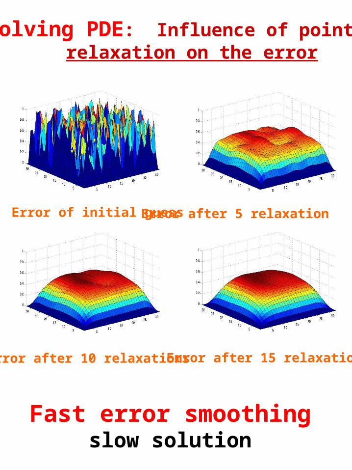
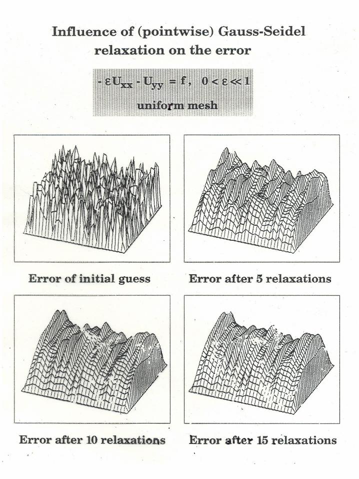
Solving PDE: Influence of pointwiserelaxation on the error
Error of initial guess Error after 5 relaxation sweeps
Error after 10 relaxations Error after 15 relaxations
Fast error smoothingslow solution

Scale-born obstacles:
• Many variables n gridpoints / particles / pixels / …
• Interacting with each other O(n2)
• Slowness
Slow Monte Carlo / Small time steps / …Slowly converging iterations /
due to
1. Localness of processing
2. Attraction basins
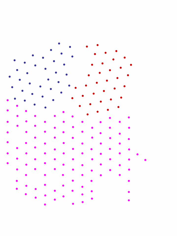
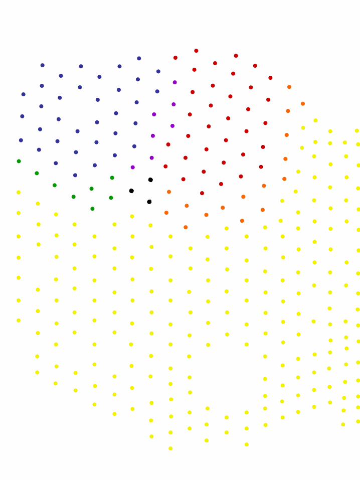
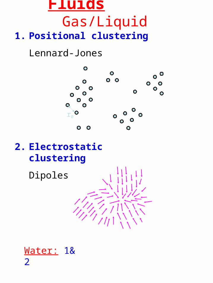
Fluids Gas/Liquid
1. Positional clustering
Lennard-Jones
r0
2. Electrostatic clustering
Dipoles
Water: 1& 2
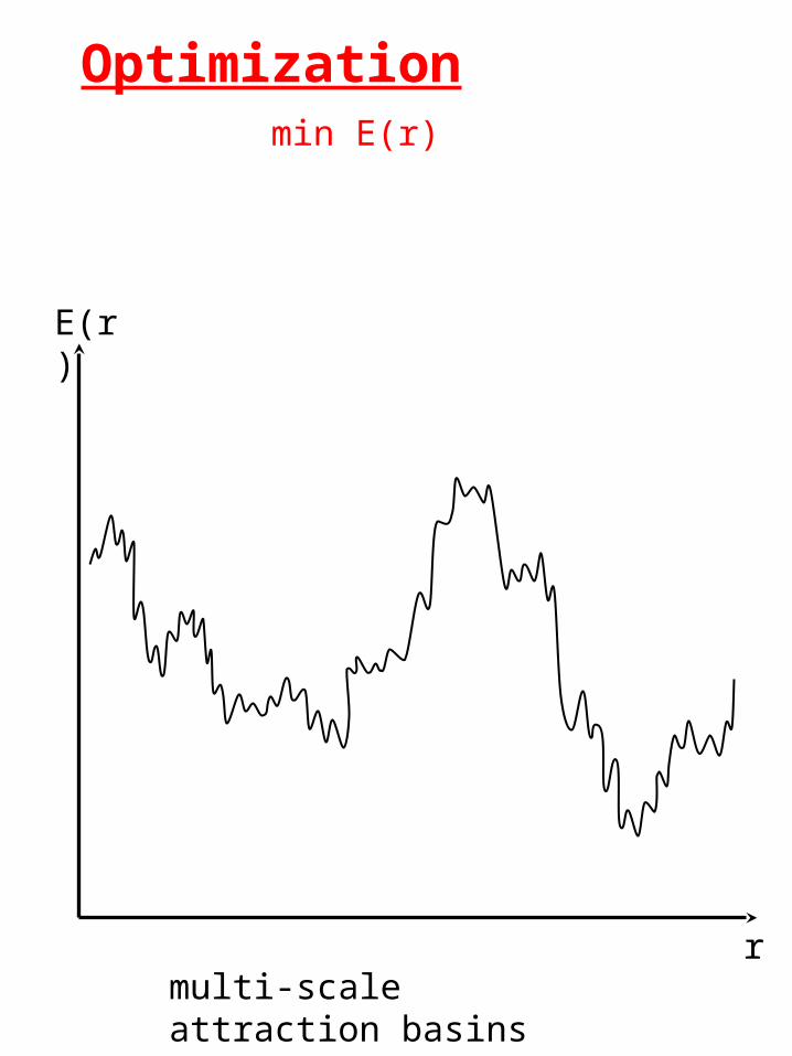
r
E(r)
Optimization min E(r)
multi-scale attraction basins

Macromolecule
+ Lennard-Jones
~104 Monte Carlo passes
for one T Gi transition
G1 G2T
Dihedral potential
+ Electrostatic

Potential Energy
S rr ,126
NBji ij
ij
ij
ij BALennard-Jones
S r
NB , j i ij
qqji Electrostatic
Bond length strain
Bond angle strain
)(1SV
DA,,,
ιjκlnijkl ncos ljki
torsion
DHA
HBAH,D, HA
HA
HA
HA 4
1210
S r
D
r
Ccos
hydrogen bond
rk
)r,...,r,r( n21E
2
,
)rr(S
S N
ijijj i
ij
2
,,
)(SKBA
ijkijk kji
ijk coscos
ijkl
ri
rjrl
rij ijk
Scale-born obstacles:
• Many variables n gridpoints / particles / pixels / …
• Interacting with each other O(n2)
• Slowness
Slow Monte Carlo / Small time steps / …Slowly converging iterations /
due to
1. Localness of processing
2. Attraction basins
Removed by multiscale processing

Solving PDE: Influence of pointwiserelaxation on the error
Error of initial guess Error after 5 relaxation sweeps
Error after 10 relaxations Error after 15 relaxations
Fast error smoothingslow solution
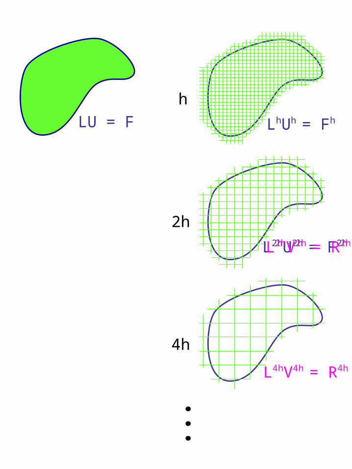
LU = F
h
2h
4h
LhUh = Fh
L2hU2h = F2h
L4hV4h = R4h
L2hV2h = R2h
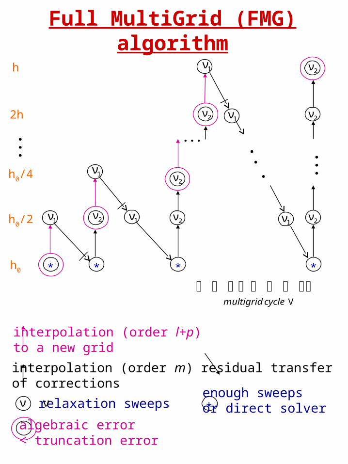
interpolation (order l+p)to a new grid
interpolation (order m)of corrections
relaxation sweeps
algebraic error< truncation error
residual transfer
ν νenough sweepsor direct solver*
**
1ν
1ν
1ν2ν
*
2ν
2ν
2ν
Full MultiGrid (FMG) algorithm
..
.
*
1ν
1ν
1ν
2ν
2ν
2ν
Vcyclemultigrid
h0
h0/2
h0/4
2h
h

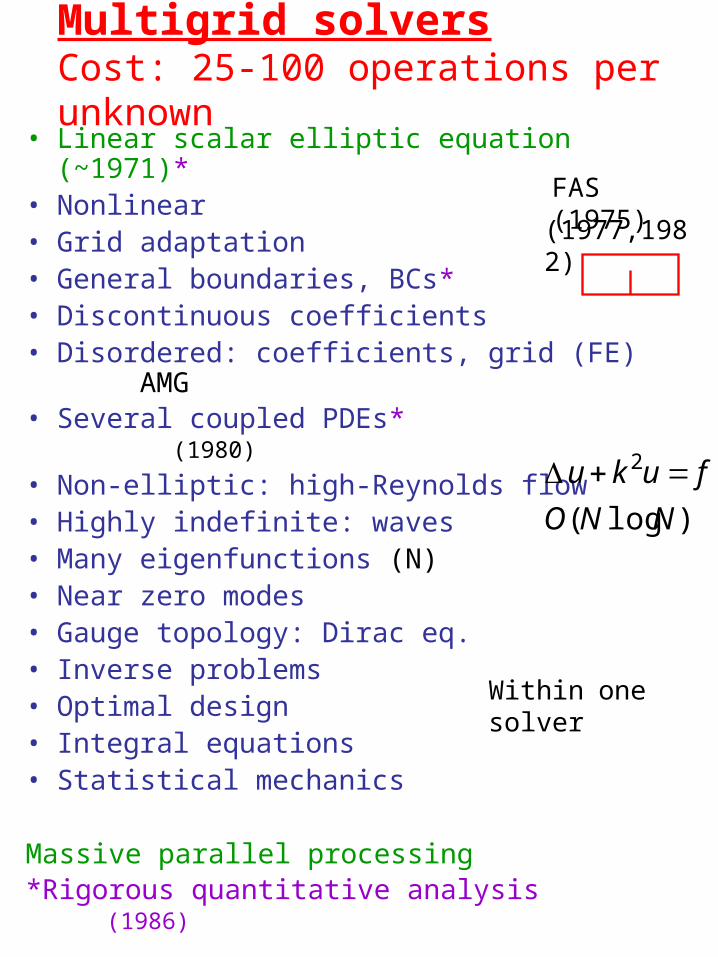
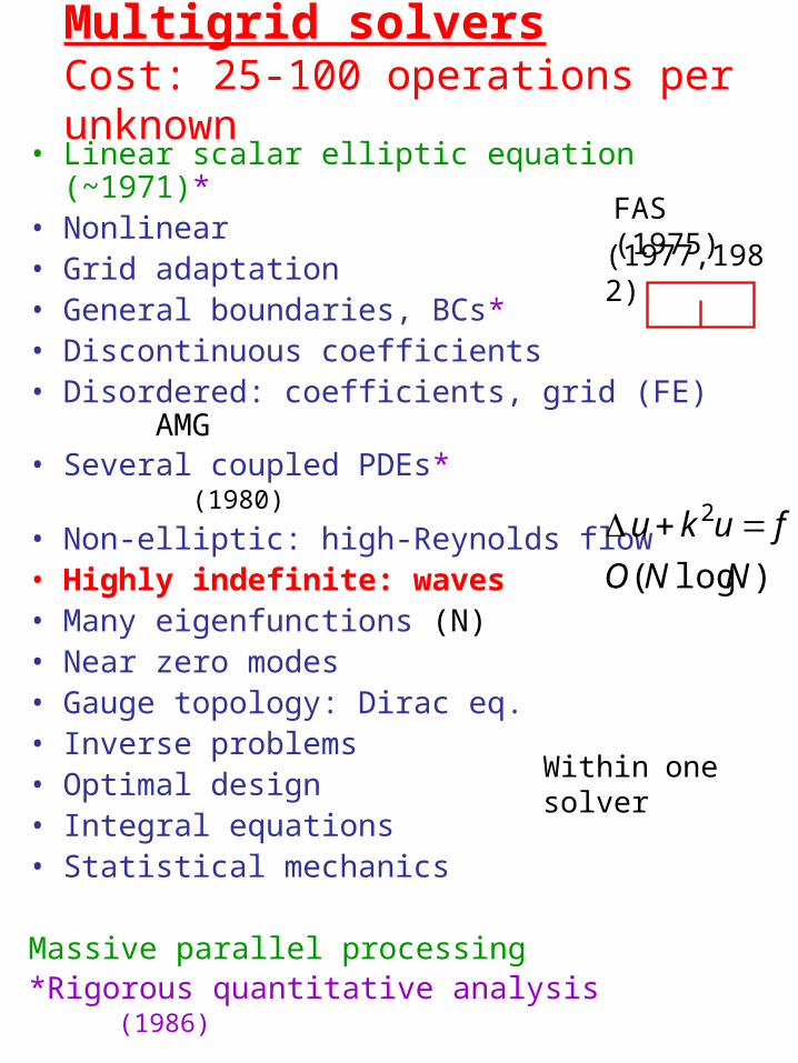
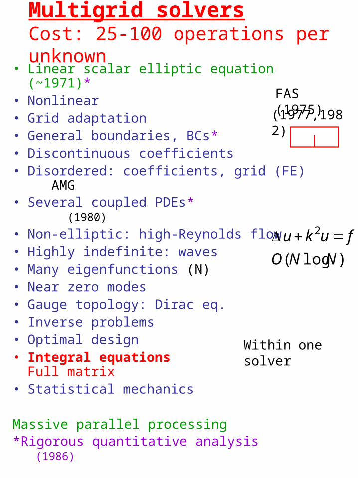
Multigrid solversCost: 25-100 operations per unknown
• Linear scalar elliptic equation (~1971)
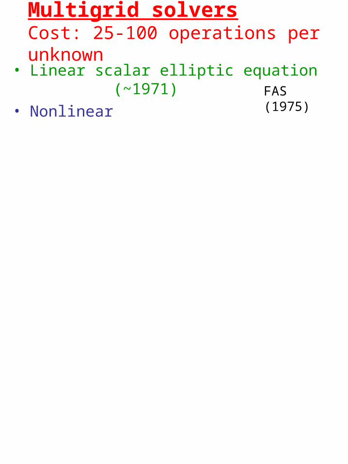
Multigrid solversCost: 25-100 operations per unknown
• Linear scalar elliptic equation (~1971)• Nonlinear FAS (1975)

LU = F
h
2h
4h
LhUh = Fh
L4hU4h = F4h
h2
h4
Fine-to-coarse defect correction
L2hV2h = R2hU2h = Uh,approximate +V2h L2hU2h = F2h
Multigrid solversCost: 25-100 operations per unknown
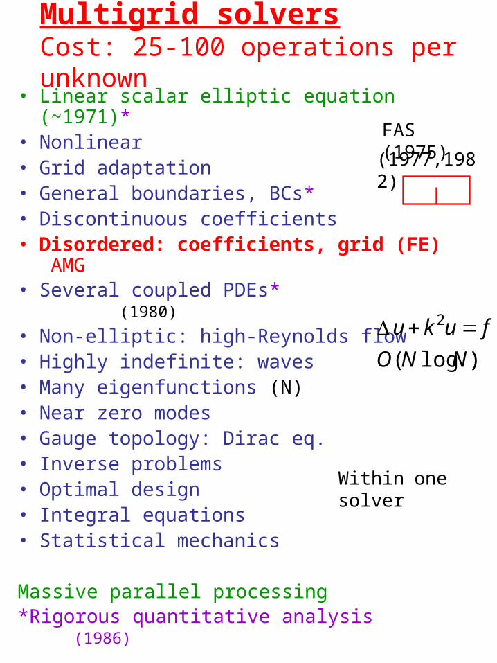
• Linear scalar elliptic equation (~1971)*• Nonlinear• Grid adaptation• General boundaries, BCs*• Discontinuous coefficients• Disordered: coefficients, grid (FE) AMG• Several coupled PDEs* (1980)
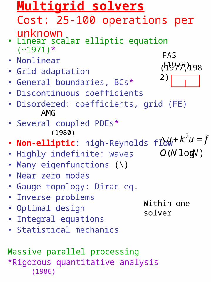
• Non-elliptic: high-Reynolds flow• Highly indefinite: waves• Many eigenfunctions (N)• Near zero modes• Gauge topology: Dirac eq.• Inverse problems• Optimal design• Integral equations• Statistical mechanics
Massive parallel processing*Rigorous quantitative analysis
(1986)
FAS (1975)
Within one solver
)log(
2
NNO
fuku
(1977,1982)

Multigrid solversCost: 25-100 operations per unknown
• Linear scalar elliptic equation (~1971)*• Nonlinear• Grid adaptation• General boundaries, BCs*• Discontinuous coefficients• Disordered: coefficients, grid (FE) AMG• Several coupled PDEs*
(1980)
• Non-elliptic: high-Reynolds flow• Highly indefinite: waves• Many eigenfunctions (N)• Near zero modes• Gauge topology: Dirac eq.• Inverse problems• Optimal design• Integral equations• Statistical mechanics
Massive parallel processing*Rigorous quantitative analysis
(1986)
FAS (1975)
Within one solver
)log(
2
NNO
fuku
(1977,1982)

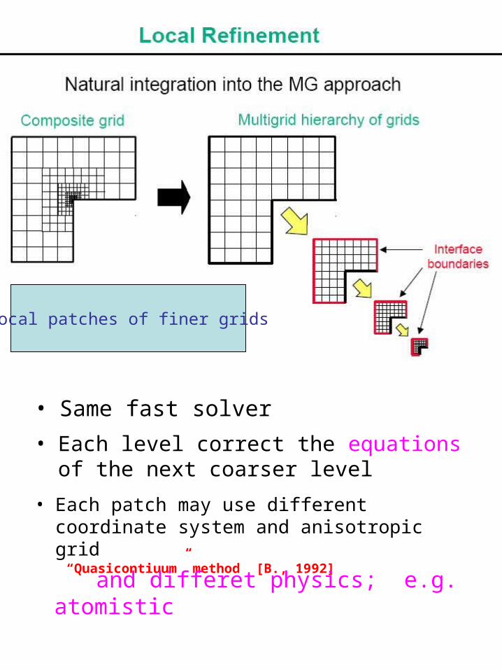
• Same fast solver
Local patches of finer grids
• Each level correct the equations of the next coarser level
• Each patch may use different coordinate system and anisotropic grid
“Quasicontiuum” method [B., 1992]
• Each patch may use different coordinate system and anisotropic grid and different
physics; e.g. Atomistic
and differet physics; e.g. atomistic
Multigrid solversCost: 25-100 operations per unknown
• Linear scalar elliptic equation (~1971)*• Nonlinear• Grid adaptation• General boundaries, BCs*• Discontinuous coefficients• Disordered: coefficients, grid (FE) AMG• Several coupled PDEs* (1980)
• Non-elliptic: high-Reynolds flow• Highly indefinite: waves• Many eigenfunctions (N)• Near zero modes• Gauge topology: Dirac eq.• Inverse problems• Optimal design• Integral equations• Statistical mechanics
Massive parallel processing*Rigorous quantitative analysis
(1986)
FAS (1975)
Within one solver
)log(
2
NNO
fuku
(1977,1982)
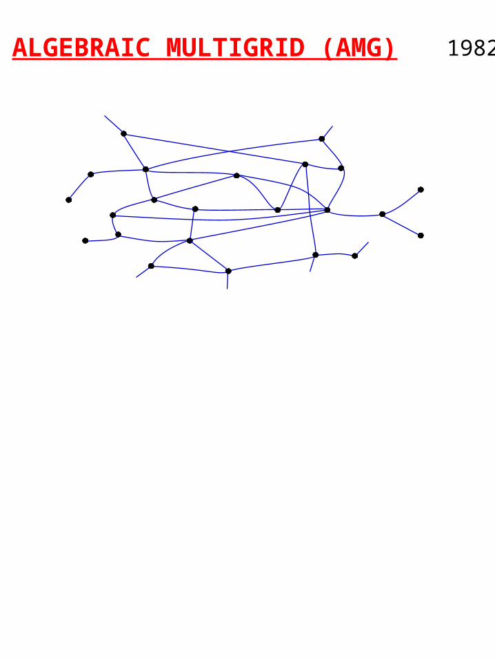
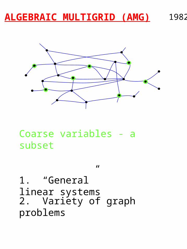
ALGEBRAIC MULTIGRID (AMG) 1982
ALGEBRAIC MULTIGRID (AMG) 1982
Coarse variables - a subset
1. “General” linear systems
2. Variety of graph problems
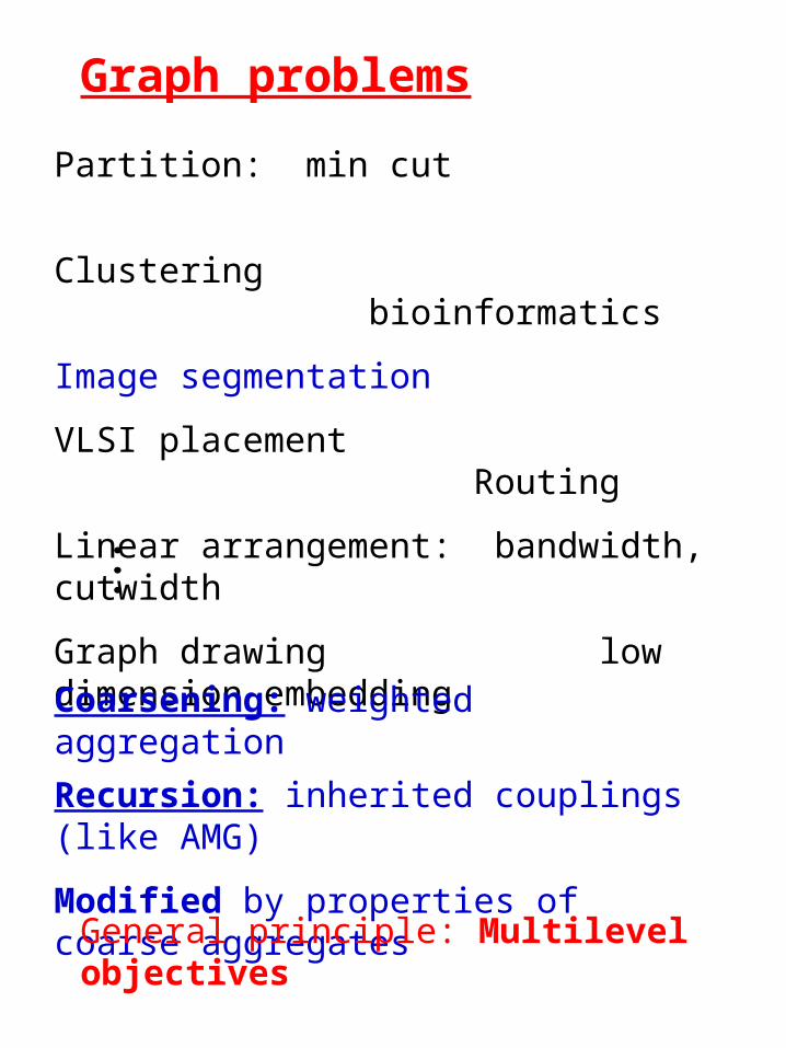
Graph problems
Partition: min cut
Clustering bioinformatics
Image segmentation
VLSI placement Routing
Linear arrangement: bandwidth, cutwidth
Graph drawing low dimension embedding
Coarsening: weighted aggregation
Recursion: inherited couplings (like AMG)
Modified by properties of coarse aggregates
General principle: Multilevel objectives
Multigrid solversCost: 25-100 operations per unknown
• Linear scalar elliptic equation (~1971)*• Nonlinear• Grid adaptation• General boundaries, BCs*• Discontinuous coefficients• Disordered: coefficients, grid (FE) AMG• Several coupled PDEs* (1980)
• Non-elliptic: high-Reynolds flow• Highly indefinite: waves• Many eigenfunctions (N)• Near zero modes• Gauge topology: Dirac eq.• Inverse problems• Optimal design• Integral equations• Statistical mechanics
Massive parallel processing*Rigorous quantitative analysis
(1986)
FAS (1975)
Within one solver
)log(
2
NNO
fuku
(1977,1982)

2h
h
2wavelength
Non-local components:
eix, ≈ ±kSlow to converge in local processing
The error after relaxationv(x) = A1(x) eikx + A2(x) e-ikx
A1(x), A2(x) smooth
Ar(x) are represented on coarser grids:
A1 + 2 i k A1′ = f1 = rh(x) e-ikx
1D Wave Equation: u”+k2u=f
k
8,8)
1,1)
2,2)3,3)
4,4)
5,5)
6,6)7,7)O(H)
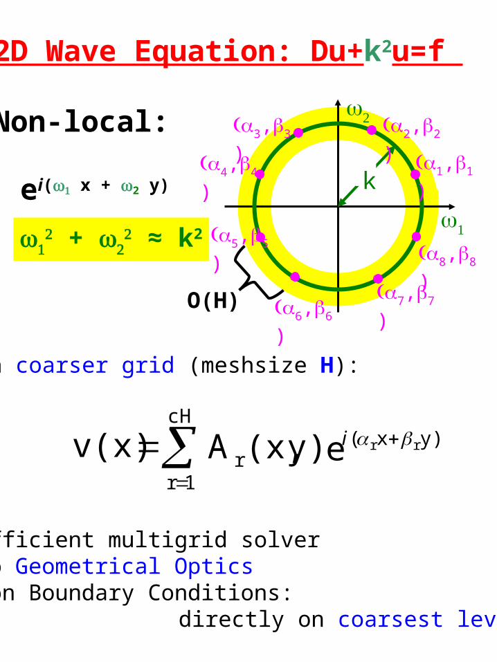
2D Wave Equation: Du+k2u=f
Non-local:
ei( x + 2 y)
+
≈ k2
On coarser grid (meshsize H):
Fully efficient multigrid solverTends to Geometrical OpticsRadiation Boundary Conditions: directly on coarsest level
cH
1r
v(x) y)(x,A ry)x( rre i
Σr = 1
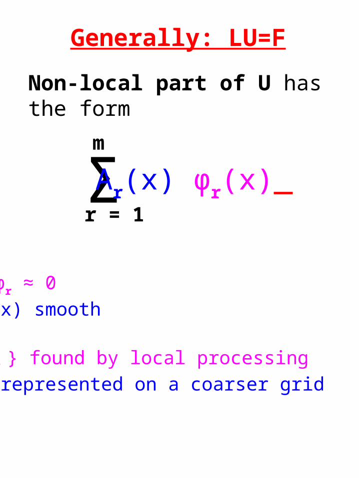
m
Ar(x) φr(x)
Generally: LU=F
Non-local part of U has the form
L φr ≈ 0
Ar(x) smooth
{φr } found by local processing
Ar represented on a coarser grid
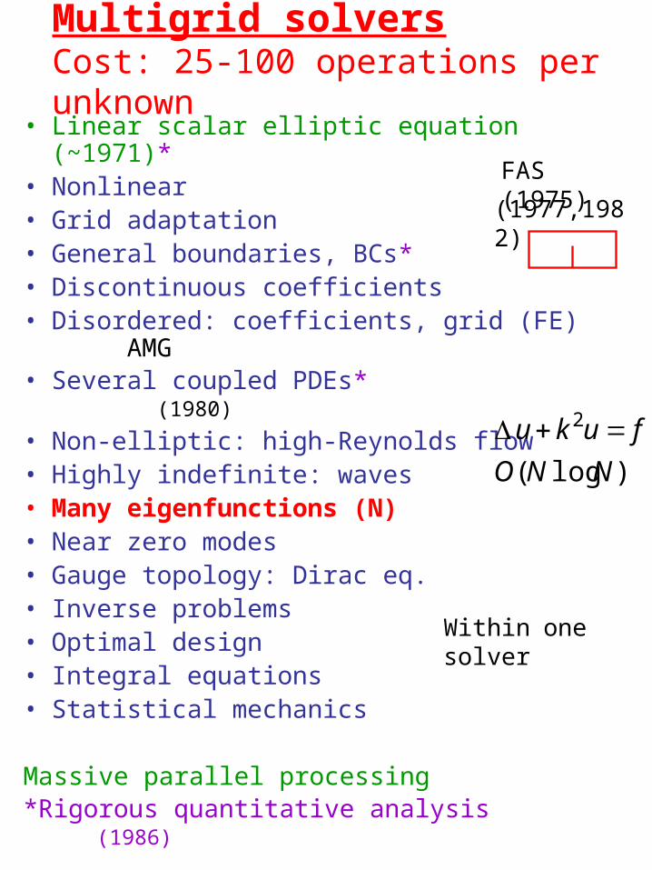
Multigrid solversCost: 25-100 operations per unknown
• Linear scalar elliptic equation (~1971)*• Nonlinear• Grid adaptation• General boundaries, BCs*• Discontinuous coefficients• Disordered: coefficients, grid (FE) AMG• Several coupled PDEs* (1980)
• Non-elliptic: high-Reynolds flow• Highly indefinite: waves• Many eigenfunctions (N)• Near zero modes• Gauge topology: Dirac eq.• Inverse problems• Optimal design• Integral equations• Statistical mechanics
Massive parallel processing*Rigorous quantitative analysis
(1986)
FAS (1975)
Within one solver
)log(
2
NNO
fuku
(1977,1982)
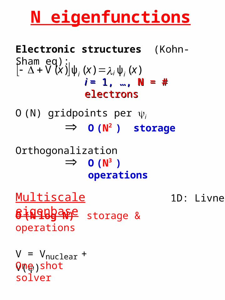
N eigenfunctions
Electronic structures (Kohn-Sham eq):
)(ψ)(ψ)(V xxx iii i i = 1, …, = 1, …, NN = # electrons= # electrons
O (N) gridpoints per i
O (N2 ) storage
Orthogonalization O (N3 ) operations
O (N log N) storage & operations
Multiscale eigenbase 1D: Livne
V = Vnuclear + V()One shot solver
Multigrid solversCost: 25-100 operations per unknown
• Linear scalar elliptic equation (~1971)*• Nonlinear• Grid adaptation• General boundaries, BCs*• Discontinuous coefficients• Disordered: coefficients, grid (FE) AMG• Several coupled PDEs* (1980)
• Non-elliptic: high-Reynolds flow• Highly indefinite: waves• Many eigenfunctions (N)• Near zero modes• Gauge topology: Dirac eq.• Inverse problems• Optimal design• Integral equations Full matrix• Statistical mechanics
Massive parallel processing*Rigorous quantitative analysis
(1986)
FAS (1975)
Within one solver
)log(
2
NNO
fuku
(1977,1982)
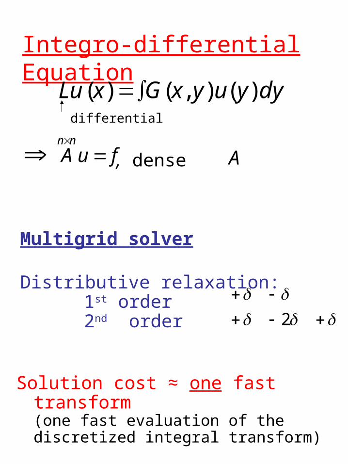
Integro-differential Equation
differential
, dense
2
dyyuyxGxLu )(),()(
fuAnn
A
Multigrid solver
Distributive relaxation:1st order2nd order
Solution cost ≈ one fast transform(one fast evaluation of the discretized integral transform)
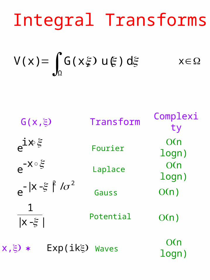
Integral Transforms
Ω
d )u( G(x, V(x) 'x
|-x|
1
/|-x|-e
x-e
ixe
22
G(x, Transform
Fourier
Laplace
Gauss
Potential
Complexity
n logn)
n logn)
n)
n)
G(x,Exp(ik Waves n logn)
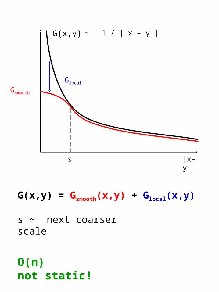
Glocal
G(x,y)
Gsmooth
s |x-y|
G(x,y) = Gsmooth(x,y) + Glocal(x,y)
s ~ next coarser scale
~ 1 / | x – y |
O(n) not static!

Multigrid solversCost: 25-100 operations per unknown
• Linear scalar elliptic equation (~1971)*• Nonlinear• Grid adaptation• General boundaries, BCs*• Discontinuous coefficients• Disordered: coefficients, grid (FE) AMG• Several coupled PDEs*
(1980)
• Non-elliptic: high-Reynolds flow• Highly indefinite: waves• Many eigenfunctions (N)• Near zero modes• Gauge topology: Dirac eq.• Inverse problems• Optimal design• Integral equations• Statistical mechanics Monte-Carlo
Massive parallel processing*Rigorous quantitative analysis
(1986)
FAS (1975)
Within one solver
)log(
2
NNO
fuku
(1977,1982)
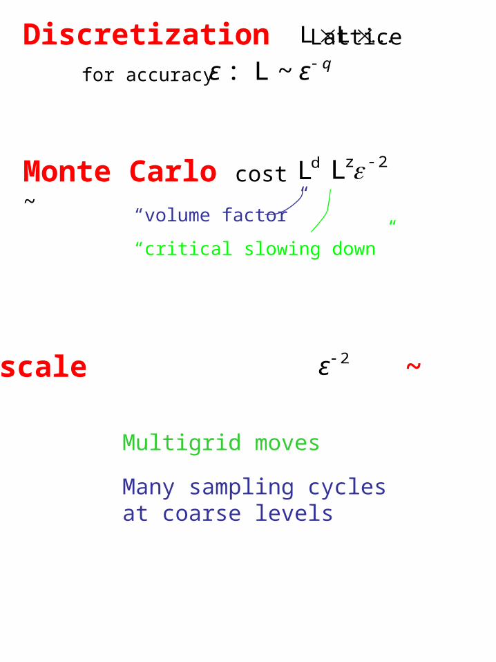
Discretization Lattice LL
for accuracy :ε qε ~L
Monte Carlo cost ~dL
“volume factor”
“critical slowing down”
Multiscale ~ 2ε
Multigrid moves
2zL
Many sampling cyclesat coarse levels
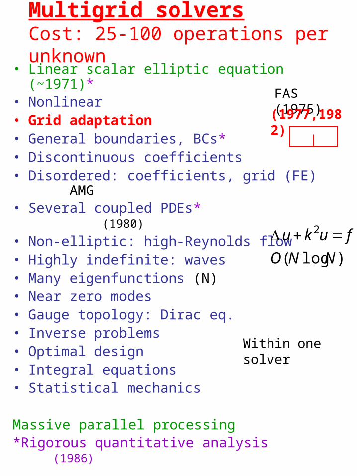
Multigrid solversCost: 25-100 operations per unknown
• Linear scalar elliptic equation (~1971)*• Nonlinear• Grid adaptation• General boundaries, BCs*• Discontinuous coefficients• Disordered: coefficients, grid (FE) AMG• Several coupled PDEs*
(1980)
• Non-elliptic: high-Reynolds flow• Highly indefinite: waves• Many eigenfunctions (N)• Near zero modes• Gauge topology: Dirac eq.• Inverse problems• Optimal design• Integral equations• Statistical mechanics
Massive parallel processing*Rigorous quantitative analysis
(1986)
FAS (1975)
Within one solver
)log(
2
NNO
fuku
(1977,1982)
• Same fast solver
Local patches of finer grids
• Each level correct the equations of the next coarser level
• Each patch may use different coordinate system and anisotropic grid
“Quasicontiuum” method [B., 1992]
• Each patch may use different coordinate system and anisotropic grid and different
physics; e.g. Atomistic
and differet physics; e.g. atomistic
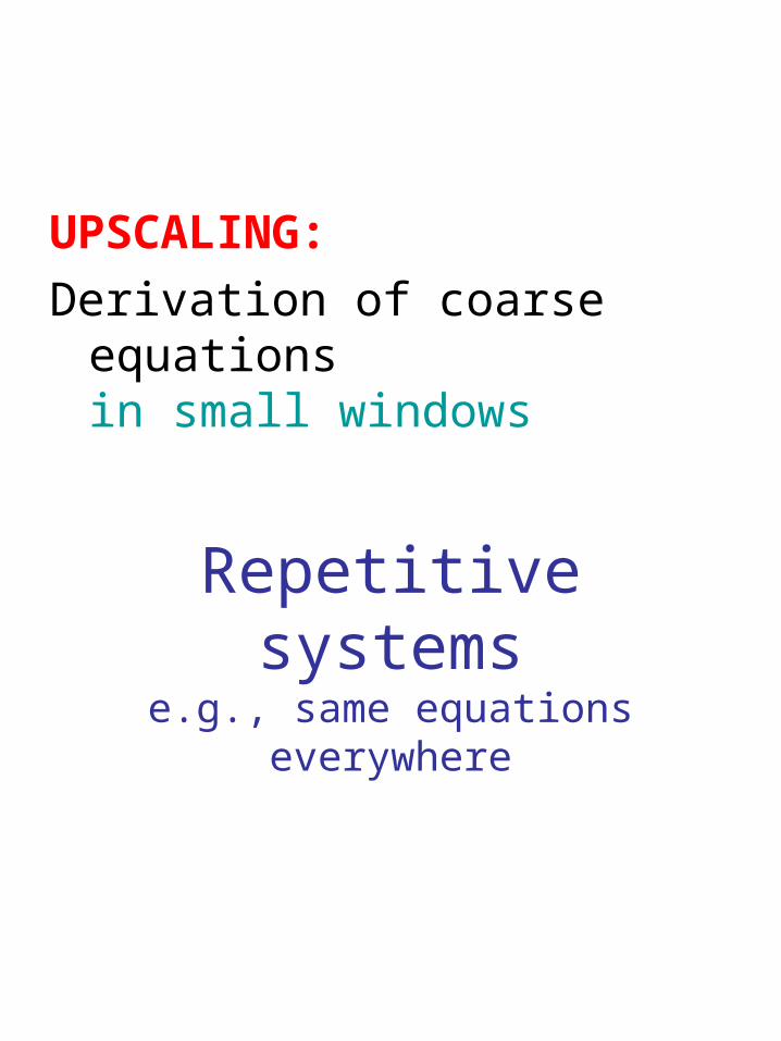
Repetitive systemse.g., same equations everywhere
UPSCALING:
Derivation of coarse equationsin small windows

Scale-born obstacles:
• Many variables n gridpoints / particles / pixels / …
• Interacting with each other O(n2)
• Slowness
Slow Monte Carlo / Small time steps / …Slowly converging iterations /
due to
1. Localness of processing
2. Attraction basins
Removed by multiscale processing

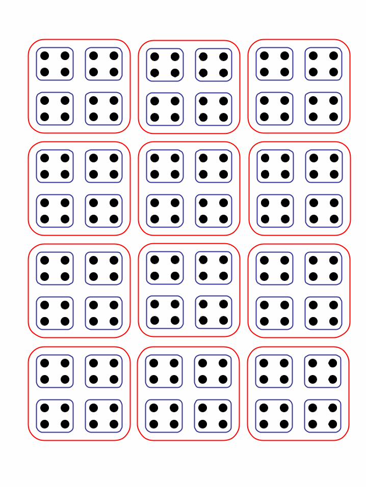
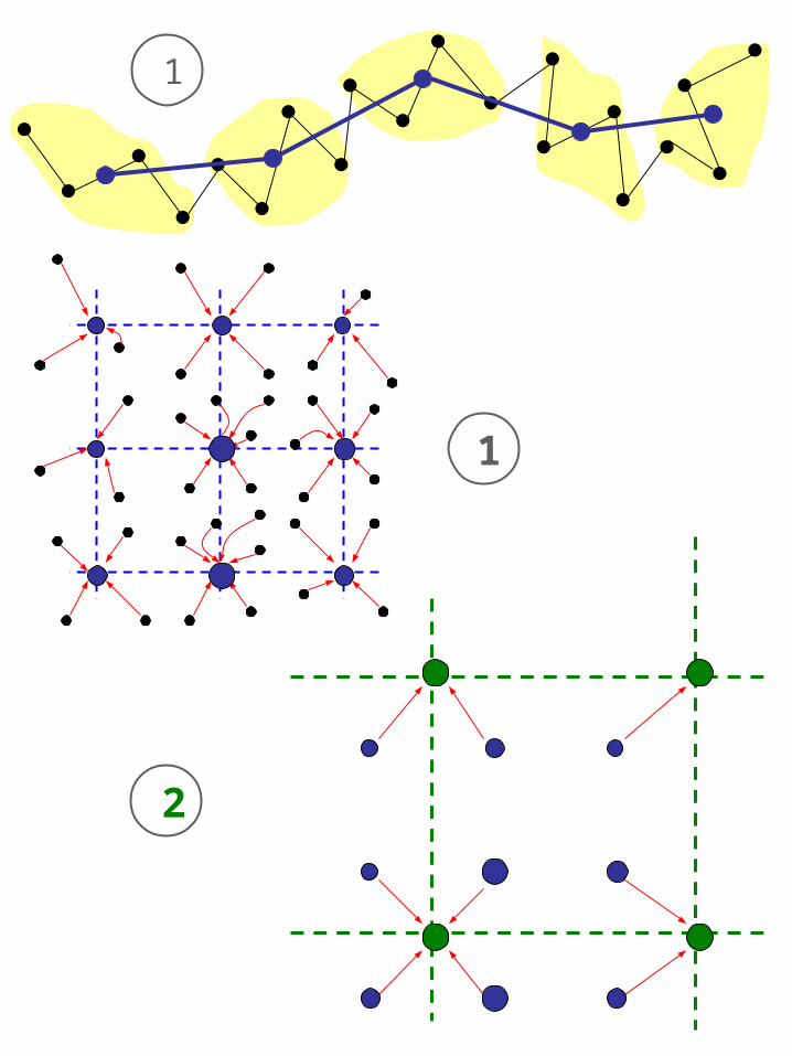
Systematic Upscaling
1. Choosing coarse variables
2. Constructing coarse-level operational rules
equations
Hamiltonian


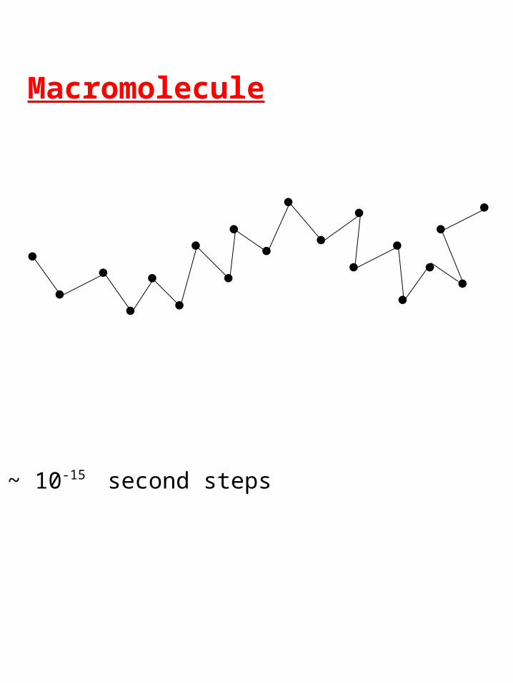
Macromolecule
~ 10-15 second steps
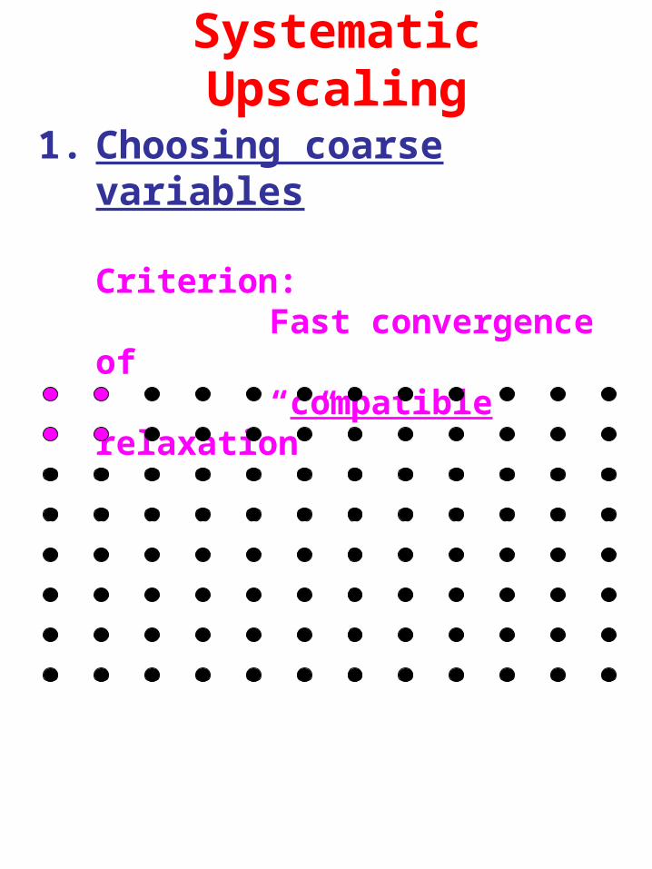
Systematic Upscaling
1. Choosing coarse variables
Criterion: Fast convergence of “compatible
relaxation”
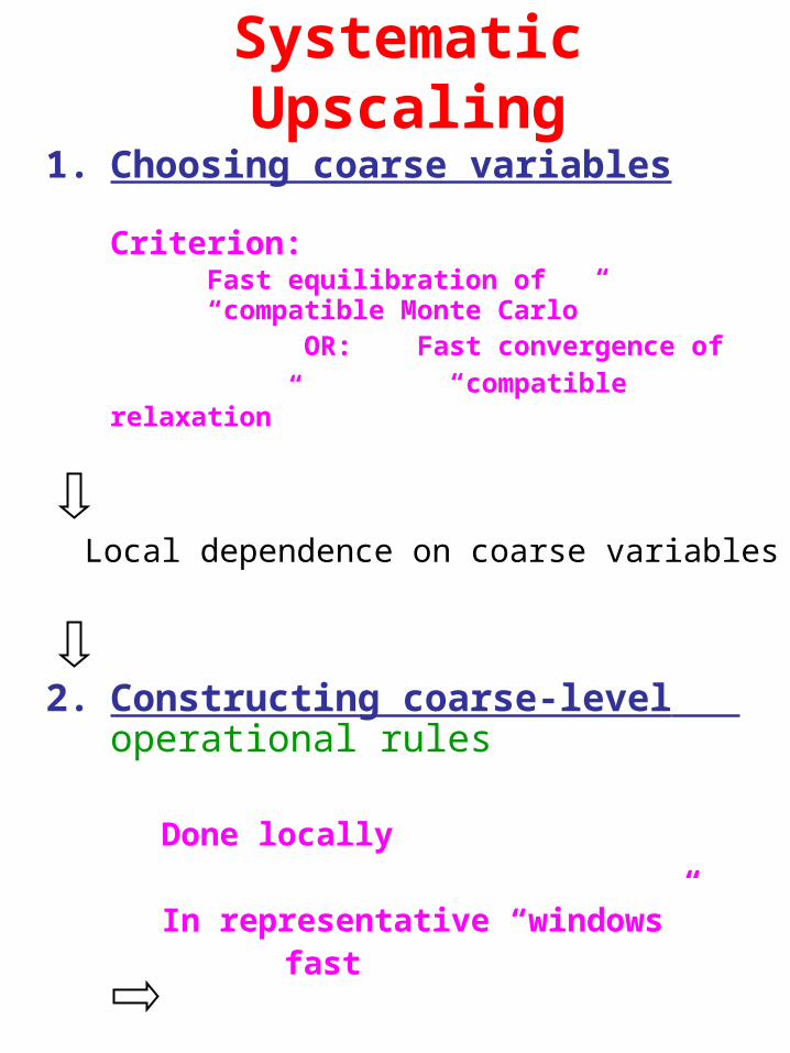
Systematic Upscaling
1. Choosing coarse variables
Criterion: Fast equilibration of “compatible Monte Carlo”
OR: Fast convergence of
“compatible relaxation”
Local dependence on coarse variables
2. Constructing coarse-level operational rules
Done locally
In representative “windows” fast
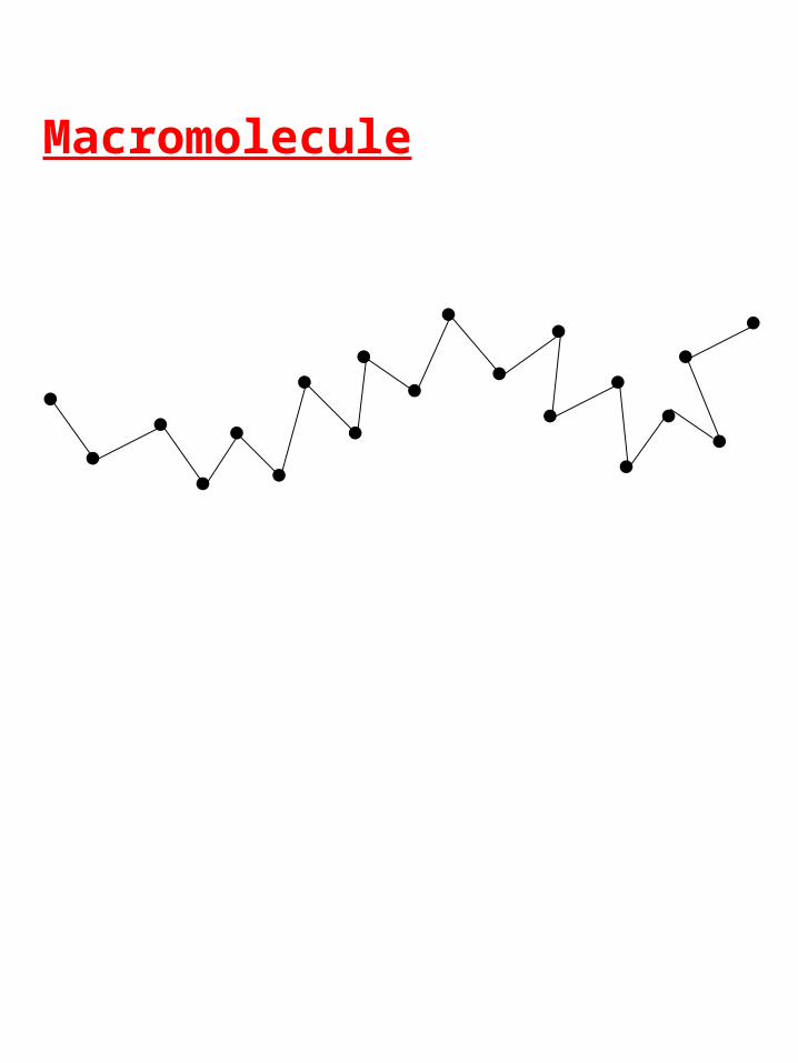
Macromolecule
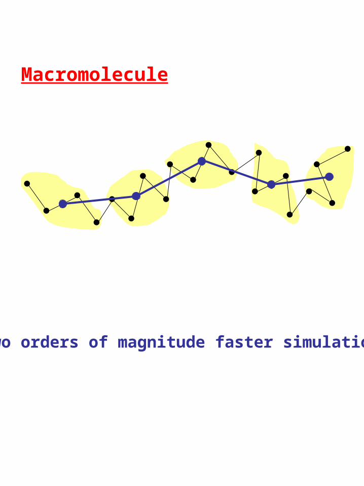
Macromolecule
Two orders of magnitude faster simulation
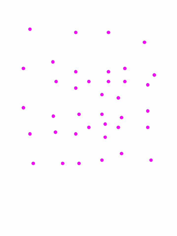
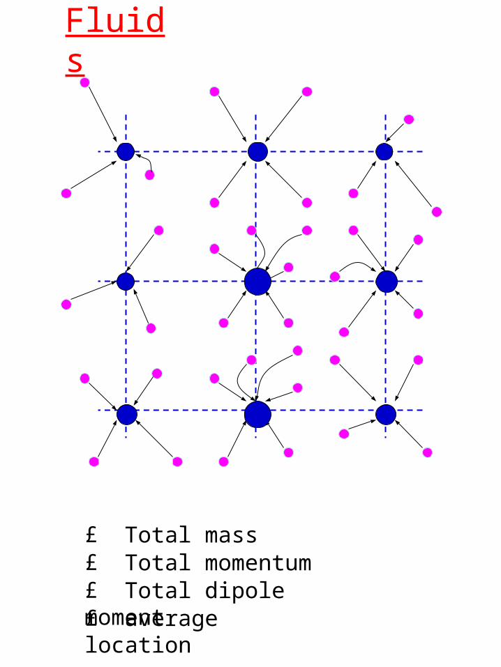
Fluids
£ Total mass£ Total momentum£ Total dipole moment£ average location
1
1
2
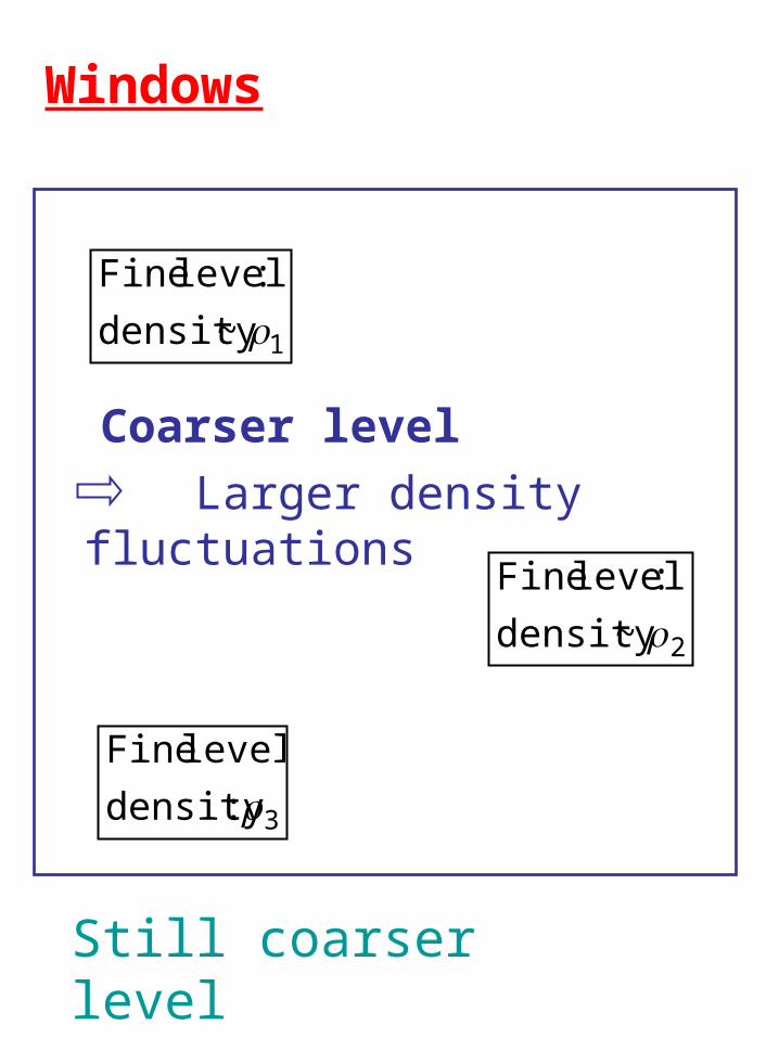
Windows
Coarser level
Larger density fluctuations
Still coarser level
1~density
:level Fine
2~density
:level Fine
3:density
level Fine

Fluids
Total mass:
)(xmSumming
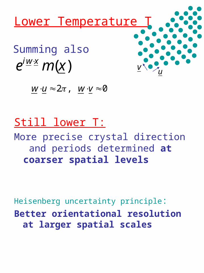
Lower Temperature T
Summing also
0 ,2 vwuw
)(xme xwi v
u
Still lower T:More precise crystal direction and
periods determined at coarser spatial levels
Heisenberg uncertainty principle:
Better orientational resolution at larger spatial scales
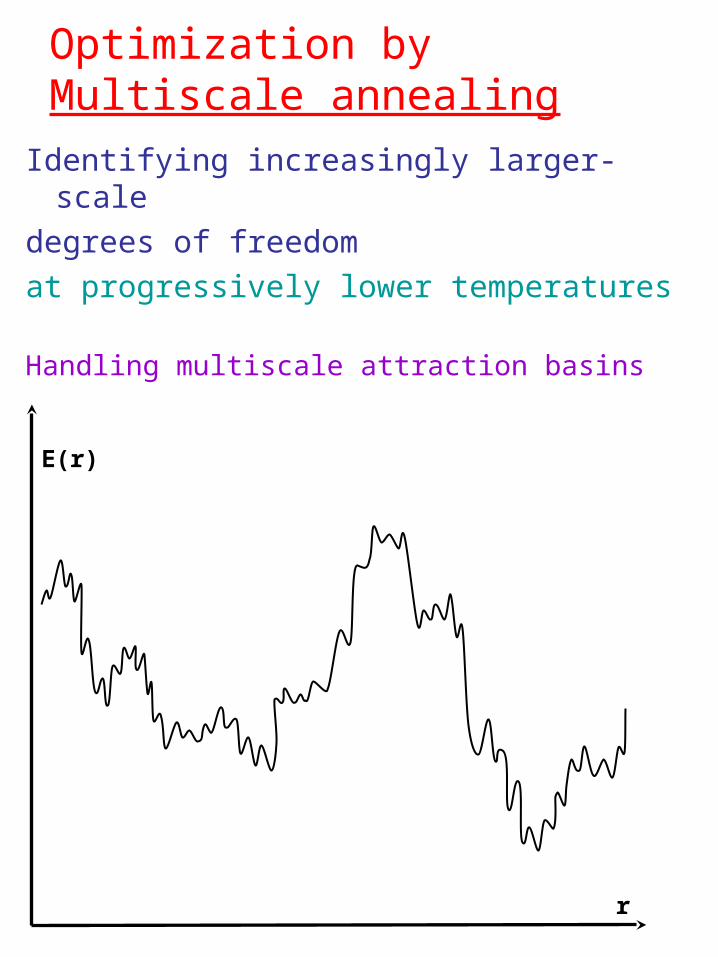
Optimization byMultiscale annealing
Identifying increasingly larger-scale
degrees of freedom
at progressively lower temperatures
Handling multiscale attraction basins
E(r)
r

Systematic Upscaling
Rigorous computational methodology to derivefrom physical laws at microscopic (e.g., atomistic) level
governing equations at increasingly larger scales.
Scales are increased gradually (e.g., doubled at each level)
with interscale feedbacks, yielding:
• Inexpensive computation : needed only in some small “windows” at each scale.
• No need to sum long-range interactions
Applicable to fluids, solids, macromolecules, electronic structures, elementary particles, turbulence, …
• Efficient transitions between meta-stable configurations.

Upscaling Projects• QCD (elementary particles):
Renormalization multigrid Ron
BAMG solver of Dirac eqs. Livne, Livshits Fast update of , det Rozantsev
• (3n +1) dimensional Schrödinger eq. Filinov
Real-time Feynmann path integrals Zlochin
multiscale electronic-density functional
• DFT electronic structures Livne, Livshits
molecular dynamics
• Molecular dynamics:
Fluids Ilyin, Suwain, Makedonska
Polymers, proteins Bai, Klug
Micromechanical structures Ghoniem defects, dislocations, grains
• Navier Stokes Turbulence McWilliams
Dinar, Diskin
1MfxM
M

THANK YOU


