Multiscale Heat, Air and Moisture Modelling and Simulation

31

Multiscale Heat, Air and Moisture Modelling and Simulation

A.W.M. van Schijndel Eindhoven University of Technology

Netherlands

1. Introduction

1.1 Background

It is widely accepted that simulation can have a major impact on the design and evaluation of building and systems performances. Also, the modelling and simulation of whole building heat, air and moisture (further-on called HAM) responses in relation to human comfort, energy and durability are relevant. IEA Annex 41 (2005) focuses on a holistic approach of HAM transfer between the outside, the enclosure, the indoor air and the heating, ventilation and air-conditioning (HVAC) systems. Therefore integrated HAM models capable of covering all these issues are sought-after. There is no single simulation tool that covers all of the issues (Augenbroe (2002)). One option is the external coupling of tools (Hensen et al. (2004); Djunaedy (2005)). Recent developments in general modelling and simulation tools give rise to another option: the use of a single computational environment. Important requirements for such a simulation environment are: a) A lot of existing HAM models are based on Ordinary Differential Equations (ODEs) or Partial Differential Equations (PDEs). Therefore it should be relative easy to implement and couple such models in the simulation environment. b) The modelling and simulation results should be reproducible and accessible. This means that the relation between mathematical model and numerical model should be clear and people in the scientific community should have access to models c) For practical use, a whole building model, capable of simulation the building response, should also be present. MatLab (including toolboxes) (2008) has become the standard tool for scientific computations. The aim of this chapter is to investigate whether the MatLab simulation environment, including SimuLink & Comsol, is capable of meeting all requirements.

1.2 HAM models

Over the past years hundreds of tools are developed (Crawley et al. (2005)). The aim of this Section is not to obtain an exhaustive list of HAM models, but to obtain a representative group of HAM models that will be used in the next Section for identifying common HAM related modelling problems. The work in this chapter is related to: (1) Annex 41 (2005), (2) building energy programs, (3) modelling and simulation techniques; (4) Matlab/SimuLink related tools. For each of the four items, a summary of involved HAM models is presented

www.intechopen.com

Recent Advances in Modelling and Simulation

608

now. First, in 2005, 14 different tools were used in an Annex 41 common exercise (2005) about simulating the dynamic interaction between the indoor climate of a room and the HAM response of the enclosure. All tools model the indoor air and the enclosure. Six HAM models are stand-alone simulation tools and have promising capabilities for simulating HVAC systems: Bsim (2008), IBPT (2008), IDA-ICE (2008), TRNSYS (2008), EnergyPlus (2008), and HAMLab (2008). The latter is presented in this chapter. Second, the energy related software tools at the Energy Tools website U.S. Department of Energy U.S (2008) has been used for several comparison studies. A recent overview is provided by Crawley et al. (2005). Furthermore, Schwab et al. (2004) used the same website for a study on programs that might simulate whole building HAM transfer. The criteria were based on: moisture storage in building materials, calculate indoor climate, moisture exchange in HVAC system, access to source code. Three tools met all criteria: Bsim (2008), TRNSYS (2008) and EnergyPlus (2008). These tools are already mentioned. Third, Gough (1999) reviews tools with the focus on new techniques for building and HVAC system modelling. In this study four simulation techniques were investigated. Proved techniques related with HAM modelling are the equation-based method techniques such as Neutral Model Format and IDA solver, which are included in IDA-ICE (2008) and TRNSYS (2008). The other mentioned techniques of Gough (1999) are simulation environments with limited HAM modelling capabilities for building simulation. Fourth, Riederer (2005) provides a recent overview of Matlab/SimuLink based tools for building and HVAC simulation. The tools who are most related with the work in this chapter are discussed now. SIMBAD (2008) provides HVAC models and related utilities to perform dynamic simulation of HVAC plants and controllers. The toolbox focuses on thermal processes with limited capabilities for moisture transport simulation. In addition to this work, this chapter presents how models that include moisture transport, can be simulated in SimuLink. The International Building Physics Toolbox (IBPT) (2008) is constructed for the thermal system analysis in building physics. The tool capabilities also include 1D HAM transport in building constructions and multi-zonal HAM calculations. (Sasic Kalagasidis (2004)). All models including the 1D HAM transport in building constructions are implemented using the standard block library of SimuLink. The developers notice the possibility to couple to other codes / procedures for 2D and 3D HAM calculations. In addition to this work, this chapter shows how this can be done using Comsol.

1.3 Common modelling problems

All HAM tools mentioned in previous Sections, face at least one limitation that cannot be solved by the tool itself. Either a problem occurs at the integration of HVAC systems models into whole building models, or a problem occurs at the integration of 2D and 3D geometry based models (for example airflow and HAM response of constructions) into whole building models. The first problem, a time scale problem, is caused by the difference in time constants between HVAC components and controllers (order of seconds) and building response (order of hours). This can cause inaccurate results and long simulation duration times (Gouda et al. (2003) and Felsman et al. (2002)). The second problem, a lumped/distributed parameters problem, is caused by the lack of lumped parameter tools to include internal 2D, 3D finite element method (FEM) capabilities (Sahlin et al. (2004)).

www.intechopen.com


609

1.4 Objectives and outline of this chapter

The key question is whether a single simulation environment is suitable for solving both the above-mentioned multi physics modelling problems concerning different time scales and lumped/distributed parameters. Our method was, first to develop, implement and validate the following modelling facilities into the simulation environment SimuLink: 1. a whole building (global) modelling facility, for the simulation of the indoor climate and

energy amounts; 2. an ordinary differential equation (ODE) solving facility, for the accurate simulation of

HVAC systems and controllers; 3. a partial differential equation (PDE) solving facility, for the simulation of 2D/3D HAM responses of building constructions and 2D internal/external airflow. The second step was to evaluate our results with regard to the key question. The outline of this chapter is as follows. Sections 2 through 4 present the integration of models into SimuLink, including validation results, concerning respectively: a whole building model (Section 2), ODE based models of HVAC and primary systems (Section 3) and PDE based models of: indoor airflow, HAM transport in constructions and external airflow/driving rain (Section 4). Finally, in Section 5, the results are discussed. At the appendix, technical details of the implementation of the models are given. This additional information provides the relation between mathematical model and code. Furthermore, it can be used as a guideline for the development of new HAM models.

2. Whole building model

Our whole building model originates from the thermal indoor climate model (ELAN) which was already published in 1987 (de Wit et al. (1988)). Separately a model for simulating the indoor air humidity (AHUM) was developed. In 1992 the two models were combined (WAVO) and programmed in the MATLAB environment (van Schijndel & de Wit (1999)). Since that time, the model has constantly been improved using newest techniques provided by recent MATLAB versions. Currently, the hourly-based model is named HAMBase, which is capable to simulate the indoor temperature, the indoor air humidity and energy use for heating and cooling of a multi-zone building. The physics of this model is extensively described by de Wit (2006). The main modeling considerations are summarized below. The HAMBase model uses an integrated sphere approach. It reduces the radiant temperatures to only one node. This has the advantage that also complicated geometries can easily be modeled. In figure 1, the thermal network is shown.

Lxa

Tx Ta

ΣΦ xy

Ca

ΣΦ ab

Φ cv-h

cvΦ

r/h

rΦ r+hcvΦ

r/hr

Figure 1. The room model as a thermal network

www.intechopen.com


610

Ta is the air temperature and Tx is a combination of air and radiant temperature. Tx is needed to calculate transmission heat losses with a combined surface coefficient. hr and hcv are the surface weighted mean surface heat transfer coefficients for convection and radiation. Φr and Φcv are respectively the radiant and convective part of the total heat input consisting of heating or cooling, casual gains and solar gains1. For each heat source a convection factor can be given. For air heating the factor is 1 and for radiators 0.5. The factor for solar radiation depends on the window system and the amount of radiation falling on furniture. Ca is the heat capacity of the air. Lxa is a coupling coefficient (Wit et al. 1988):

⎟⎟⎠⎞⎜⎜⎝

⎛+=

r

cvcvtxa

h

hhAL 1 (1)

∑Φab is the heat loss by air entering the zone with an air temperature Tb. At is the total area. In case of ventilation Tb is the outdoor air temperature. ∑Φxy is transmission heat loss through the envelope part y. For external envelope parts Ty is the sol-air temperature for the particular construction including the effect of atmospheric radiation. The admittance for a particular frequency can be represented by a network of a thermal resistance (1/Lx) and capacitance (Cx) because the phase shift of Yx can never be larger than π/2. To cover the relevant set of frequencies (period 1 to 24 hours) two parallel branches of such a network are used giving the correct admittance's for cyclic variations with a period of 24 hours and of 1 hour. This means that the heat flow Φxx(tot) is modeled with a second order differential equation. For air from outside the room with temperature Tb a loss coefficient Lv is introduced. The model is summarized in figure 2

Lxa

Lx2

Lx1

CaCx2Cx1

Τb

ΔΦxy

Φp1

Φg1

Tx Ta

Φp2 Φg2

TyLvLyx

Figure 2. The thermal model for one zone

In a similar way a model for the air humidity is made. Only vapour transport is modeled, the hygroscopic curve is linearized between RH 20% and 80%. The vapour permeability is

1 Please note that the model presented in figure 1 is a result of a delta-star transformation.

www.intechopen.com


611

assumed to be constant. The main differences are: a) there is only one room node (the vapour pressure) and b) the moisture storage in walls and furniture, carpets etc is dependent on the relative humidity and temperature.

2.1 Integration and the time scale problem

It is obvious that the hourly based approach of HAMBase is not accurate enough if we want to integrate building systems with its relative small time scales (order seconds). Our major recent improvement is the development of a so called hybrid model that consists of both a continuous part with a variable time step as well as a discrete part with a time step of one hour. We adapted our HAMBase model by splitting the energy and vapor flows into two parts. First, a discrete part was developed for modelling the transmittance through walls. Second, a continuous part was developed for the rest (admittance, ventilation, sources, etc.). We implemented this approach by using so-called S-Functions for SIMULINK (see also the Appendix). This new model, named HAMBASE_S to avoid confusion, is able to simulate complicated HVAC installations and controls simultaneously with the building. We summarize the main advantages: a. The dynamics of the building systems where small time scales play an important role

(for example on/off switching) are accurately simulated. b. The model becomes time efficient as the discrete part uses 1-hour time steps. A yearly

based simulation takes less than 3 minutes on a Pentium 3.4 GHz, 2GB computer. c. The moisture (vapor) transport model of HAMBase is also included. With this feature,

the (de-) humidification of HVAC systems can also be simulated.

2.2 Verification

2.2.1 Standard test (thermal)

The Bestest (ASHRAE, (2001)) is a structured approach to evaluate the performance of building performance simulation tools. The evaluation is performed by comparing results of the tested tool relative to results by reference tools. The procedure requires simulating a number of predefined and hierarchal ordered cases. Firstly, a set of qualification cases have to be modelled and simulated. If the tool passes all qualification cases the tool is considered to perform Bestest compliant. In case of compliance failure the procedure suggests considering diagnostic cases to isolate its cause. Diagnostic cases are directly associated with the qualification cases (Judkoff and Neymark 1995). The first qualification case, case 600 (see figure 3) was used for the performance comparison.

Figure 3. Bestest Case Geometry

www.intechopen.com


612

The thermal part of HAMBase has been subjected to a standard method of test (Bestest ASHRAE, (2001)) with satisfactory results. For further details, see Table 1.

CASE NR. SIMULATION OF MODEL RESULT MIN.TEST MAX. TEST

600ff mean indoor temperature [oC] 25.1 24.2 25.9

600ff min. indoor temperature [oC] -17.9 -18.8 -15.6

600ff max. indoor temperature [oC] 64.0 64.9 69.5

900ff mean indoor temperature [oC] 25.1 24.5 25.9

900ff min. indoor temperature [oC] -5.1 -6.4 -1.6

900ff max. indoor temperature [oC] 43.5 41.8 44.8

600 annual sensible heating [MWh] 4.9 4.3 5.7

600 annual sensible cooling [MWh] 6.5 6.1 8.0

600 peak heating [kW] 4.0 3.4 4.4

600 peak sensible cooling [kW] 5.9 6.0 6.6

900 annual sensible heating [MWh] 1.7 1.2 2.0

900 annual sensible cooling [MWh] 2.6 2.1 3.4

900 peak heating [kW] 3.5 2.9 3.9

Table 1. Comparison of the room model with some cases of the standard test

2.2.2 Parameter sensitivity test (thermal)

The Bestest case 600 is used to study uncertainties by Hopfe et al. (2007). Uncertainties have been assigned to 48 input parameters describing the physical properties of the case and its operation. The input parameters used are exactly the same for three tools, IESVE, VA114

www.intechopen.com


613

and HAMBase. The model parameters are normally distributed using a fixed standard deviation of 5% for all variables. A standard deviation of 5% does not represent a realistic parameter uncertainty but defines a common base for the tool performance comparison. For each input parameter 200 samples were generated by latin hypercube sampling. The prototypes were deployed to generate simulation input files from the sample matrix and run the simulations. Figure 4 shows the parameter sensitivities for the annual sensible heating (case 600) produced by the four tools.

2.0000

2.5000

3.0000

3.5000

4.0000

4.5000

5.0000

5.5000

6.0000

6.5000

1 6

11

16

21

26

31

36

41

46

51

56

61

66

71

76

81

86

91

96

Number of simulations

An

nu

al h

eati

ng

[ M

Wh

]

IES LEA VA114 HAMBase

Figure 4. Parameter sensitivity test for four building energy simulation tools

Figure 4 shows a very good agreement between the IESVE and HAMBase tools. This is remarkable because both tools have quite different modeling approaches. We may conclude both modeling approaches give similar results for the considered case studies.

2.2.3 Annex 41 test (hygric)

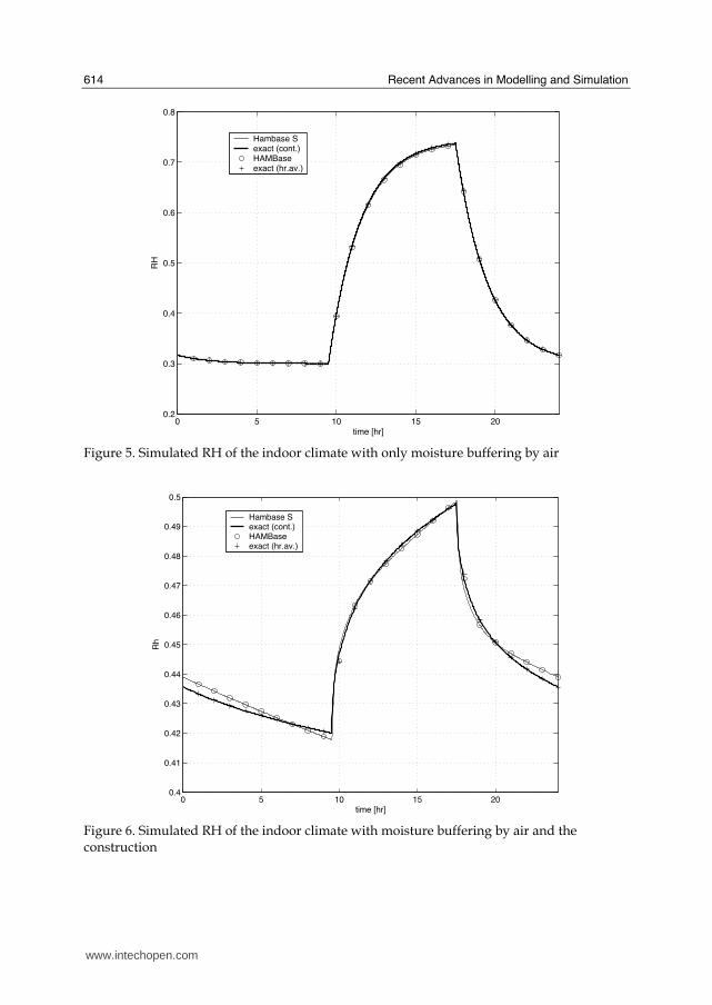
The hygric parts of both HAMBase and HAMBase_S have been subjected to a new benchmark case developed by the IEA Annex 41 (2005). The geometry is identical to the Bestest (ASHRAE standard (2001)). Further test conditions are as follows: (1) there is only one 1D construction type with linear properties; (2) the exposure is completely isothermal; (3) the outside relative humidity (RH) is 30%; (4) there are no windows; (5) the internal gains equal 500g/hour; (6) the ventilation rate is 0.5 ach. Bednar & Hagentoft (2005) provide the analytical solution of this benchmark. Figure 5 and 6 show the results of the two benchmarks representing moisture buffering by air alone and by combined air and the construction.

www.intechopen.com


614

0 5 10 15 200.2

0.3

0.4

0.5

0.6

0.7

0.8

time [hr]

RHHambase Sexact (cont.)HAMBaseexact (hr.av.)

Figure 5. Simulated RH of the indoor climate with only moisture buffering by air

0 5 10 15 200.4

0.41

0.42

0.43

0.44

0.45

0.46

0.47

0.48

0.49

0.5

time [hr]

Rh

Hambase Sexact (cont.)HAMBaseexact (hr.av.)

Figure 6. Simulated RH of the indoor climate with moisture buffering by air and the construction

www.intechopen.com


615

Both figures provide four results: the hourly and continuous analytical solution of Bednar & Hagentoft (2005), the hourly based HAMBase solution and the continuous HAMBase_S solution. The results show a good agreement between all solutions.

2.3 Validation

The intention of the following study, developed within the Annex 41, was to retrieve an experimental based and well defined benchmark for evaluating the involved HAM models. The experiment comprehends two real and almost identical rooms, which are located at the outdoor testing site of the Fraunhofer-Institute of building physics in Holzkirchen. During the winter of 2005-2006, tests were carried out. The walls and the ceiling of the test room were fully covered with aluminum foil. In the reference room 50 m2 of the walls was not covered with aluminum providing more buffering capacity of the walls compared to the test room. The air temperature in both rooms was kept between 19.8 and 20.2 oC. The next results are presented: the measured and simulated RH in the reference room (figure 7) and heating power to the reference room (figure 8).

Figure 7. The measured and simulated RH in the reference room

www.intechopen.com


616

Figure 8. The measured and simulated heating power in the reference room

The results of the test room are similar to the reference room and are therefore left out. The results from figure 7 and 8 show a good agreement between measured and simulated results. We may conclude that our approach of discrete/continuous modelling provide accurate results within acceptable simulation duration times and thus providing us a good solution to the mentioned time scale problem.

3. ODE based modelling

Often, mathematical models of HVAC and primary systems and controllers can be expressed as a system of Ordinary Differential Equations (ODEs). In this Section we present the integration of ODE based models into SimuLink and thus providing a coupling between building and systems.

3.1 Integration

A complete case study on how to integrate a model described by a system of ODEs into SimuLink is now exemplarily shown for a heat pump model. We start with a mathematical model of the heat pump, based on first principles, in the form of ODEs:

www.intechopen.com


617

⎢⎢⎢⎢⎢⎢⎢

⎣

⎡

⋅−−−⋅⋅=

⋅+−⋅⋅=

⋅+⋅−⋅+⋅

+⋅+⋅⋅=

hpvoutvinwvinvout

v

hpcoutcinwcincout

c

voutvincoutcin

coutcin

E1)(COP)T(TcFdt

dTC

ECOP)T(TcFdt

dTC

)T0.5T(0.5)T0.5T(0.5

273.15T0.5T0.5kCOP

(2)

Where T is temperature [oC], COP Coefficient of Performance [-], k heat pump efficiency [-], cw specific heat capacity of water [J/kgK], C heat capacity of the water and pipes in the heat pump [J/K], t time[s], F mass flow [kg/s], Ehp heat pump electric power supply [W]. Subscript c means water at the condenser, v water at the evaporator, in, incoming, out, outgoing. The second step is to define the input-output definition of the model. The final step is to implement the mathematical model into a S-Function, a programmatic description of a dynamic system. The technical details of the last two steps are presented in the Appendix. The importance of these details is that the relation between mathematical model and implemented model is clear and it is very useful for developers who want to create their own ODE based models. It should be mentioned that the time scale problem seems less relevant in case of ODE based models because there are special designed solvers for this case. So-called stiff solvers can handle such a problem accurately and time efficient. On the other hand, simulating controllers for example (rapid) on/off switching can generate small time steps during simulation. Although accurate results are obtained in this case, it could still lead to relative long simulation duration times.

3.2 Validation

At a test site of the Eindhoven University, a configuration with a heat pump, an energy roof and a thermal energy storage has been investigated with a focus on the convective heat recovery from ambient air. Also one of the goals of this project was to evaluate the modelling approach of previous Section applied to respectively a heat pump, an energy roof and a thermal energy storage. From this work, published in van Schijndel & de Wit (2003c), we show the validation results of the heat pump which are presented in figure 9. In this figure the measured and simulated water temperatures of the outgoing flows at the condenser and evaporator are compared and show a good agreement. The other components: energy roof and thermal energy storage were validated with similar results. We may conclude that the presented ODE based modelling approach provide accurate results. In general it is expected that systems modeled as a system of ODEs can be relative easy and accurately simulated using the presented modelling approach.

www.intechopen.com


618

Figure 9. The measured and simulated water temperature of the evaporator (top) and condenser (bottom)

4. PDE based modelling

HAM responses of building constructions and internal/external airflow can be modeled and simulated with Comsol (formerly FemLab) (2008). This is an environment for modelling scientific and engineering applications based on partial differential equations (PDEs). Comsol [Comsol 2006] is a toolbox which solves systems of coupled PDEs (up to 32 independent variables). The specified PDEs may be non-linear and time dependent and act on a 1D, 2D or 3D geometry. The PDEs and boundary values can be represented by two forms. The coefficient form is as follows2

Ω=+∇+−+∇⋅∇−∂

∂infuauuuc

t

uda βγα )( (3a)

Ω∂−=+−+∇⋅ onguquucn λγα )( (3b)

2 * The symbols provided by the Comsol modeling guides are also used here.

www.intechopen.com


619

Ω∂= onruh (3c)

The first equation (3.1a) is satisfied inside the domain Ω and the second (3.1b) (generalized Neumann boundary) and third (3.1c) (Dirichlet boundary) equations are both satisfied on the boundary of the domain Ω. n is the outward unit normal and is calculated internally. λ is an unknown vector-valued function called the Lagrange multiplier. This multiplier is also calculated internally and will only be used in the case of mixed boundary conditions. The coefficients da , c, α , ß, , a, f, g, q and r are scalars, vectors, matrices or tensors. Their components can be functions of the space, time and the solution u. For a stationary system in coefficient form da = 0. Often c is called the diffusion coefficient, α and ß are convection coefficients, a is the absorption coefficient and and f are source terms. The second form of the PDEs and boundary conditions is the general form:

ΩinFΓt

uda =⋅∇+

∂

∂ (4a)

ΩonλGΓn ∂+=⋅− (4b)

Ωon0R ∂= (4c)

The coefficients Γ and F can be functions of space, time, the solution u and its gradient. The components of G and R can be functions of space, time, and the solution u. Given the geometry, an initial finite element mesh is automatically generated by triangulation of the domain. The mesh is used for discretisation of the PDE problem and can be modified to improve accuracy. The geometry, PDEs and boundary conditions are defined by a set of fields similarly to the structure in the language C. A graphical user interface is used to simplify the input of these data. For solving purposes Comsol contains specific solvers (like static, dynamic, linear, non-linear solvers) for specific PDE problems.

4.1 HAM models and validation

In (Comsol 2006) examples are already present which show the accuracy and reliability of Comsol. However there are no validations for typical building physics problems. Specific for validating building physics simulations in Comsol, this Section deals with two (very different) time dependent non-linear problems. Each problem is solved and compared with measured data.

4.1.1 1D Moisture transport in a porous material

The water absorption in an initially dry brick cylinder (length 24-mm) is studied. All sides except the bottom are sealed. This side is submerged in water at t=0 sec. The PDE and boundary conditions for this problem are:

www.intechopen.com


620

0.024xon0x

θ0,xon0.27θ

0.024,x0onθ))(D(θt

θ

==∂

∂

==

<<∇⋅∇=∂

∂

(5)

The coefficient form (3) is used. The results of measured water absorption of several brick materials based on (Brocken 1998) are shown in figure 10, left hand side. The moisture profiles are shown versus lambda (lambda is defined by the position divided by the square root of the time). For each material the diffusivity as a function of the moisture content is given [Brocken 1998] and used to simulate the corresponding profiles.

Figure 10. Measured and simulated moisture content profiles versus lambda of the 1D moisture transport problem. Left hand side: Measured moisture contents, Right hand side: Simulated moisture contents

The simulation results in figure 10, right hand side, are compared with the measured profiles3.

3 Such a comparison is used to gain confidence in the model and simulation tool.

www.intechopen.com


621

4.1.2 2D Airflow in a room

This example from Sinha (2000) deals with the velocity and temperature distribution in a room heated by a warm air stream. In figure 11 the geometry and boundary conditions are presented.

Figure 11. The geometry and boundary conditions for the 2D-airflow problem The problem is modelled by 2D incompressible flow using the Boussinesq approximation with constant properties for the Reynolds and Grasshof numbers. U-momentum equation

ux

p

y

vu

x

uu

t

u 2

Re

1)()(∇+

∂

∂−

∂

∂−

∂

∂−=

∂

∂

V-momentum equation

TGr

vy

p

y

vv

x

uv

t

v2

2

ReRe

1)()(+∇+

∂

∂−

∂

∂−

∂

∂−=

∂

∂

Continuty equation (6)

0=∂

∂+

∂

∂

y

v

x

u

Energy equation

Ty

vT

x

uT

t

T 2

PrRe

1)()(∇+

∂

∂−

∂

∂−=

∂

∂

The general form (4a-c) is used for this type of non-linear problem. In (Sinha 2000) the problem is solved and validated with measurements for several combinations of Re and Gr. In figure 12 these results are presented.

The boundary conditions are: At the left, right, top and bottom walls: u=0, v=0, T=0. At the inlet: u=1, v=0, T=1. At the outlet : Neuman conditions for u,v and T

www.intechopen.com


622

0 0.5 1 1.5 2 2.50

0.5

1

1.5

2

2.5

3

0.

0.1

0.2

0.2

0.3

0.3

0.4

0.4

0.5

0.5

0.6

0.6

0.7

0.7

0.8

0.8 0.9

0 0.5 1 1.5 2 2.50

0.5

1

1.5

2

2.5

3 0.1

0.1

0.2

0.2

0.3

0.3

0.4

0.4

0.4

0.5

0.5

0.6

0.6

0.7

0.7

0.8

0.8

0.9

0.9

0 0.5 1 1.5 2 2.50

0.5

1

1.5

2

2.5

3

0

0.1

0

0.2

0

0.3

0.

0.4

0.4

0.5

0.5

0.5

0.6

0.6

0.6 0.7

0.7

0.7

0.7

0.8

0.8

0.9

0.9

Figure 12. Dimensionless temperature contours comparison of the validated simulation results of [Sinha 2000] (left hand side) with the Comsol results (right hand side) for the 2D-airflow problem

www.intechopen.com


623

The left-hand side shows the results obtained by (Sinha 2000) and the right side show the corresponding Comsol results. The verification results are satisfactory.

4.1.3 2D wind surrounding a building and driving rain

In addition to the above mentioned models, a new developed model concerning driving rain is presented now. The model is verified by another benchmark case of the mentioned IEA Annex 41 (2005), on boundary conditions. The benchmark covers for several building geometries: (a) Simulated wind velocity profiles around buildings; (b) Simulated raindrop trajectories; (c) Simulated wind-driving-rain coefficients on the building facades. The solution of (a) is obtained by using the standard k-epsilon turbulence model of Comsol. Figure 13 shows the simulated wind profile around the lower building.

Figure 13. The wind velocity profile: absolute value of the velocity [m/s] for each coordinate x, y [m]

The solution of (b) is obtained from the equation of motion of a raindrop (Gunn & Kinzer (1949)), moving in a wind-flow field characterized by a velocity vector v:

2

2

)(Re),(dt

rd

dt

drvCdfg =−⋅+ (7)

where g is gravity, f is a function dependent on Re (Reynolds number) and Cd (drag coefficient), v is wind velocity, t is time and r is the position of raindrop. Equation 2 is solved with the ODE solver of MatLab providing raindrop trajectories. The result for the low building benchmark case is shown in figure 14.

www.intechopen.com


624

Figure 14. The raindrop trajectories

The solution of (c) is obtained from the locations of raindrops hitting the building façade. The preliminary results are in good agreement with the results obtained by a reference solution. This is shown in figure 15.

Figure 15. Wind-driven rain coefficient at the centre of the building (reference solution: 3D CFD, our solution: 2D CFD)

www.intechopen.com


625

4.1.4 Full 3D HAM modeling study

This Section demonstrates the integration of a 3D HAM model of a roof/wall construction into a whole building model. The geometry of the building is identical to one in [ASHRAE 2001]. HAMBase SimuLink is used as whole building model. Figure 16 shows the input/output structure of the integrated model.

Figure 16. Input/output structure of the SimuLink model

The output (air temperature and RH) of this model and climate data are used as input for the Comsol model of a 3D roof/wall construction. The output of the Comsol model (heat and moisture flow) is connected to the input of the building model. The Comsol model is similar to the model presented in Section 3.4. Figure 17 and 18 demonstrate the 3D temperature and vapour distributions at a specific time.

Figure 17. The temperature distribution: temperature [oC] for each coordinate x, y, z [m]

www.intechopen.com


626

Figure 18. The vapour pressure distribution: vapour pressure [Pa] for each coordinate x, y, z [m]

The integrated model is capable of simulating the indoor climate and construction details within reasonable simulation time: 1 year simulation, takes about 12 hours of computation time (Pentium 4, 500MB)

4.1.5 Discussion on reliability

The test cases in this Section show that Comsol is very reliable even for a highly non-linear problem such as convective airflow. Furthermore, for all the simulation results presented in this chapter, the default mesh generation and solver are used. So good results can be obtained without a deep understanding of the gridding and solving techniques. The simulation times (based on processor Pentium 3, 500 MHz) ranged from fast (order ~seconds) for linear problems such as the 2D thermal bridge example, medium (order ~minutes) for non linear problems in the coefficient form such as the 1D moisture transport example to high (order ~hours) for highly non linear problems in the general form such as the airflow problem.

4.2 Integration and the lumped/distributed parameter problem

A second new development concerns the integration of a distributed parameter model and lumped parameter model in SimuLink. In this case study, the 2D airflow model of van Schijndel is implemented using the discrete part of an S-function. After each time step (in this case 1 sec) the solution is exported. Dependent on the controller, different boundary values can be applied. Furthermore, the airflow at the inlet is now controlled by an on/off controller with hysteresis (Relay) of SimuLink. The sensor temperature (lumped parameter) is calculated as mean of a several air temperature nodes (distributed parameter). If the temperature of the sensor above 20.5 oC the air temperature at the inlet is 17 oC if the air temperature is below 19.5 oC the inlet temperature is 22 oC. Initially the inlet temperature is 18 oC. Figure 19 gives an overview of the results.

www.intechopen.com


627

Figure19. Part A, The SimuLink model including the S-function of the Comsol model and controller (Relay), Part B, the temperature of the sensor (-) and the output of the on/off controller (+) versus time, Part C, the air temperature distribution at 8 sec. (hot air is blown in) and Part D, the air temperature distribution at 10 sec. (cold air is blown in) (o = sensor position)

Again the technical details are provided at the Appendix. From figure 19, it is clear that the controller has a great impact on the indoor airflow dynamics and temperature distribution. Many researchers perhaps overlook this phenomenon because most of the time, quasi steady airflow is assumed. This also shows the need of integrated models as presented here. Furthermore, we compared the amount of computational time used for solving the airflow problem to the rest of processes including calculation of the lumped parameter and the on/off controller. It turned out (as expected) that in this case most of the time (>98%) was consumed for solving exclusively the airflow problem.

www.intechopen.com


628

5. Conclusion

It is concluded that the presented simulation environment Matlab/SimuLink/Comsol is capable of solving a large range of integrated HAM problems. Furthermore, it seems promising in accurately solving modelling problems that are caused by the presence of different time scales and/or lumped/distributed parameters. However, there are some limitations: (1) some specific solvers such as time-dependent k-epsilon turbulence solvers are not available yet. This means that, for example, time dependent 3D airflow around buildings cannot be integrated without external coupling; (2) Although it is possible to construct a full 3D integrated HAM model of the indoor air and all constructions in the simulation environment, the simulation duration time would probably be far too long to be of any practical use; (3) The modelling of radiation is not included in this research. The main benefits of our modelling approach are: (1) it takes advantage of the facilities of the well maintained Matlab/SimuLink and Comsol simulation environment such as the state-of-art ODE/PDE solvers, controllers library, graphical capabilities etc; (2) all presented models in this chapter are public domain; (3) although not explicitly shown in this chapter, compared to other HAM models, it is relative easy to integrate new models that are based on ODEs and/or PDEs. (4) the simulation facilitates open source modelling and if desired, models can be compiled into stand-alone (web) applications.

6. References & tools

Augenbroe, G. (2002). Trends in building simulation, Building and Environment 37, pp.891-902

ASHRAE (2001). Standard method of test for the evaluation of building energy analysis computer programs, standard 140-2001.

Bednar, T. & C.E. Hagentoft. (2005). Analytical solution for moisture buffering effect; Validation exercises for simulation tools. Nordic Symposium on Building Physics, Reykjavik 13-15 June 2005 pp. 625-632

Brocken, H., 1998, Moisture transport in brick masonry, Ph.D. thesis, Eindhoven University of Technology

Clarke J.A. (2001). Domain integration in building simulation, Building and Environment 33, pp. 303-308

Crawley, D.B., Hand, J.W. Kummert, M. & Griffith B. (2005). Contrasting the capabilities of building performance simulation programs, 9TH IBPSA Conf. Montreal pp 231- 238

Djunaedy, E. (2005) External coupling between building energy simulation and computational fluid dynamics. PhD thesis, Technische Universiteit Eindhoven

Felsmann C., Knabe G., Werdin H. (2002). Simulation of domestic heating systems by integration of TRNSYS in a MATLAB/SIMULINK model, Proc. 6TH Int. Conference System Simulation in Buildings Liege, December 16-18

Gouda M.M., Underwood C.P., Danaher S. (2003). Modelling the robustness properties of HVAC plant under feedback control, Building Serv. Eng. Res. Techn. 24,4 pp. 271-280

Gough M.A. (1999). A review of new techniques in building energy and environmental modelling, No. BREA-42. Garston, Watford, UK: Building Research Establishment.

Gunn, R. & G.D. Kinzer (1949). The terminal velocity of fall for water droplets in stagnant air. Journal of Meteorology 6 pp. 243-248

www.intechopen.com


629

Hagentoft C.E. and 13 other authors. (2002). HAMSTAD – Final Report,, Report R-02:8, Chalmers Univ. of Tech., Sweden

Hensen, E. Djunaedy, M. Radosevic, A. Yahiaoui. (2004), Building performance simulation for better design: some issues and solutions, 21TH PLEA Conference Eindhoven, pp.1185-1190

Christina Hopfe, Christian Struck1, Petr Kotek, Jos van Schijndel1, Jan Hensen and Wim Plokker (2007) uncertainty analysis for building performance simulation; a comparison of four tools Proceedings: Building Simulation 2007

IEA Annex 41 (2005). http://www.ecbcs.org/annexes/annex41.htm Judkoff, R. and Neymark, J. (1995). International energy agency building energy simulation

test (BESTEST) and diagnostic method, National Renewable Energy Laboratory, Golden, CO.

Kunzel H.M., (1996). IEA Annex 24 HAMTIE, Final Report – Task 1 Rieder P. (2005) MatLab/SimuLink for building and HVAC simulation – state of art. 9TH Int.

IBPSA Conference Montreal 2005, pp1019-1026 Sasic Kalagasidis, (2004) HAM-Tools; An Integrated Simulation Tool for Heat, Air and

Moisture Transfer Analyses in Building Physics, PhD thesis, Chalmers Univ. of Techn.

Sahlin P. Eriksson L., Grozman P., Johnson H., Shapovalov A. Vuolle M.( 2004). Whole-building simulation with symbolic DAE equations and general purpose solvers. Building and Environment 39, pp. 949-958.

Schellen, H.L. (2002), Heating Monumental Churches, Indoor Climate and Preservation of Cultural heritage; PhD thesis, Eindhoven University of Technology.

Schijndel, A.W.M. van & Wit, M.H. de, (1999), A building physics toolbox in MatLab, 7TH Symposium on Building Physics in the Nordic Countries Goteborg, pp81-88

Schijndel A.W.M. van (2003a). Modeling and solving building physics problems with FemLab, Building and Environment 38, pp 319-327

Schijndel A.W.M. van, Schellen, H.L., Neilen D. (2003b). Optimal setpoint operation of the climate control of a monumental church, 2ND international conf. on research in building physics, Leuven, Sept. 14-18 2003, pp. 777-784

Schijndel A.W.M. van, Wit M.H. de (2003c). Advanced simulation of building systems and control with SimuLink, 8TH IBPSA Conference Eindhoven. pp. 1185-1192

Schijndel, A.W.M. van (2003d). Integrated building physics simulations with FemLab/SimuLink /Matlab, 8TH Int. IBPSA Conference, Eindhoven, pp. 1177-1184

Schijndel A.W.M. van 2004. Advanced use of HAMLab on CE1, Annex 41 preliminary chapter TUE Oct 2004 Chapter A41-T1-NL-04-5, available in 2008.

Schijndel A.W.M. van, Schellen H.L. (2005). Application of an integrated indoor climate & HVAC model for the indoor climate design of a museum, submitted for the 7TH symposium on building physics in the Nordic Countries, 13-15 June 2005, Iceland

Schijndel A.W.M. van (2007), Integrated Heat Air and Moisture Modeling and Simulation, PhD thesis, Eindhoven University of Technology, ISBN: 90-6814-604-1, 200 pages

Schwab M. and Simonson C.J. 2004. Review of building energy simulation tools that include moisture storage in building materials and HVAC systems, Annex 41 preliminary chapter A41-T2-C-04-6, available in 2008.

Sinha S.L. 2000. Numerical simulation of two-dimensional room air flow with and without buoyancy, Energy and Buildings 32 pp121-129

www.intechopen.com


630

U.S. Department of Energy, 2008 http://www.eere.energy.gov/ Wit M.H. de ,H.H. Driessen 1988, ELAN A Computer Model for Building Energy Design.

Building and Environment, Vol.23,4, pp. 285-289 Wit, M.H. de, 2006, HAMBase, Heat, Air and Moisture Model for Building and Systems

Evaluation, Bouwstenen 100, ISBN 90-6814-601-7 Eindhoven University of Technology

BSIM 2008. http://www.bsim.dk/ COMSOL 2008. http://www.comsol.com/ Energyplus 2008. http://www.eere.energy.gov/ Fluent 2008. http://www.fluent.com/ HAMLab 2008. http://sts.bwk.tue.nl/hamlab/ IES VE 2008 http://www.iesve.com IBPT 2008. http://www.ibpt.org/http://www.iesve.com IDA ICE 2008. http://www.equa.se/ice/intro.html Matlab 2008. http://www.mathworks.com/ SIMBAD 2008. http://software.cstb.fr/ TRNSYS 2008. http://sel.me.wisc.edu/trnsys/ VABI 2008 http://www.vabi.nl/

7. Appendix

In the appendix, technical details of the implementation of the models are given. This additional information provides the relation between mathematical model and code needed to reproduce our results. A complete example how to model a system of ODEs with an S-function of SimuLink is shown for the heat pump model. The first step is to define the input-output definition of the model. This is presented in Table 2.

Name Input (u) / Output (y)

Description

Tvin u(1) Incoming water temperature at the evaporator [oC]

Fvin u(2) Incoming mass flow at the evaporator [kg/s]

Tcin u(3) Incoming water temperature at the condenser [oC]

Fcin u(4) Incoming mass flow at the condenser [kg/s]

Ehp u(5) Power of electrical supply [W]

k u(6) efficiency [-]

Tvout y(1) Outgoing water temperature at the evaporator [oC]

Tcout y(2) Outgoing water temperature at the condenser [oC]

COP y(3) Coefficient Of Performance [-]

Table 2. The input-output definition of the heat pump model

The second step is to formulate a mathematical model by a system of ODEs. This is done using (1). The third step is to implement the mathematical model into a S-function, a programmatic description of a dynamic system. Details about this subject can be found in MatLab 2008. Figure 20 shows the corresponding SimuLink model. Figure 21 provides the complete program code.

www.intechopen.com


631

Figure 20. The input-output structure in SimuLink

Figure 21. The contents of the S-Function for the heat pump model

The main part of program code (with comments) to integrate an airflow model into SimuLink using a S-functions is provided in figure 22.

function [sys,x0,str,ts] = wpsfun2(t,x,u,flag) %WPSFUN2 Heat pump %u(1)=Tvin [oC], u(2)=Fvin [kg/s], u(3)=Tcin [oC], %u(4)=Fcin [kg/s], u(5)=Ehp [W], u(6)=k [-] %y(1)=Tvout [oC] (=x(1)), y(2)=Tcout [oC] (=x(2)) %y(3)=COP switch flag … end

function [sys,x0,str,ts]=mdlInitializeSizes sizes.NumContStates = 2; % Number of Cont. states sizes.NumDiscStates = 0; % Number of Disc. states sizes.NumOutputs = 3; % Number of Outputs sizes.NumInputs = 6; % Number of Inputs x0 = [10; 10]; % Initial values

function sys=mdlDerivatives(t,x,u) Tvm=(u(1)+x(1))/2; Tcm=(u(3)+x(2))/2; COP=u(6)*(273.15+Tcm)/(Tcm-Tvm); Cc=200000;Cv=200000;cv=4200;cc=4200; xdot(1)=(1/Cv)*(u(2)*cv*(u(1)-x(1))-(COP-1)*u(5)); xdot(2)=(1/Cc)*(u(4)*cc*(u(3)-x(2))+COP*u(5)); sys = [xdot(1); xdot(2)];

function sys=mdlOutputs(t,x,u) Tvm=(u(1)+x(1))/2; Tcm=(u(3)+x(2))/2; COP=u(6)*(273.15+Tcm)/(Tcm-Tvm); sys = [x(1); x(2); COP];

www.intechopen.com


632

Figure 22. Example of the implementation of a Comsol model in the discrete section of a S-function of SimuLink

function [sys,x0,str,ts] = dsfun(t,x,u,flag) % t: time; x = state vector ; u = input vector; % flag = control parameter by SimuLink global OutT Outsol % specify variable 'fem': the Comsol model geomtry, mesh, % PDE coefficents and boundary conditions switch flag, case 0, [sys,x0,str,ts] = mdlInitializeSizes(fem,tstap,u0);% Initialization % case 2, sys = mdlUpdate(t,x,u,fem,tstap); %update discrete part case 3, sys = mdlOutputs(t,x,u,fem,tstap); %produce output case 9, sys = []; %terminate end %end dsfunc function [sys,x0,str,ts] = mdlInitializeSizes(fem,tstap,u0) global OutT Outsol % calculated the next values needed for SimuLink % calculated initial values for time OutT(1) and % initial values for solution Outsol(1) % x0 are all values of the temperature on the mesh OutT(1)=0; Outsol(1)=x0; function sys = mdlUpdate(t,x,u,fem,tstap) global OutT Outsol if u(1)>0.5 % if dimensionless Temperature of sensor > 0.5 then fem.bnd.r= '-u1'; '-u2' ;0 ; '0-u4' ... %boundary value cold air else fem.bnd.r= '-u1'; '-u2' ;0 ; '1-u4' ... % bounadry value hot air end tijd=[t; t+tstap/2; t+tstap]; %calculate simulatetime for Comsol model fem.sol=femtime(fem,'atol',.1,.1,Inf,.1,'ode','fldae',... 'sd','on','report','on','tlist',tijd,'init',x); %simulate airflow OutT=[OutT (t+tstap)]; % update time Outsol=[Outsol fem.sol.u(:,ntijd)]; % update solution function sys = mdlOutputs(t,x,u,fem,tstap) global OutT Outsol Points=[69 84 101 167 188 211 259 261]; % location of sensor in mesh sys=mean(x(Points)); % output

www.intechopen.com

Modelling and SimulationEdited by Giuseppe Petrone and Giuliano Cammarata

ISBN 978-3-902613-25-7Hard cover, 688 pagesPublisher I-Tech Education and PublishingPublished online 01, June, 2008Published in print edition June, 2008

InTech EuropeUniversity Campus STeP Ri Slavka Krautzeka 83/A 51000 Rijeka, Croatia Phone: +385 (51) 770 447 Fax: +385 (51) 686 166www.intechopen.com

InTech ChinaUnit 405, Office Block, Hotel Equatorial Shanghai No.65, Yan An Road (West), Shanghai, 200040, China

Phone: +86-21-62489820 Fax: +86-21-62489821

This book collects original and innovative research studies concerning modeling and simulation of physicalsystems in a very wide range of applications, encompassing micro-electro-mechanical systems, measurementinstrumentations, catalytic reactors, biomechanical applications, biological and chemical sensors,magnetosensitive materials, silicon photonic devices, electronic devices, optical fibers, electro-microfluidicsystems, composite materials, fuel cells, indoor air-conditioning systems, active magnetic levitation systemsand more. Some of the most recent numerical techniques, as well as some of the software among the mostaccurate and sophisticated in treating complex systems, are applied in order to exhaustively contribute inknowledge advances.

How to referenceIn order to correctly reference this scholarly work, feel free to copy and paste the following:

A.W.M. van Schijndel (2008). Multiscale Heat, Air and Moisture Modelling and Simulation, Modelling andSimulation, Giuseppe Petrone and Giuliano Cammarata (Ed.), ISBN: 978-3-902613-25-7, InTech, Availablefrom:http://www.intechopen.com/books/modelling_and_simulation/multiscale_heat__air_and_moisture_modelling_and_simulation

© 2008 The Author(s). Licensee IntechOpen. This chapter is distributedunder the terms of the Creative Commons Attribution-NonCommercial-ShareAlike-3.0 License, which permits use, distribution and reproduction fornon-commercial purposes, provided the original is properly cited andderivative works building on this content are distributed under the samelicense.

https://creativecommons.org/licenses/by-nc-sa/3.0/

Date post:	11-Feb-2022
Category:	Documents
Upload:	others
View:	9 times
Download:	0 times

Multiscale Heat, Air and Moisture Modelling and Simulation

Documents