Multiscale inference for multivariate deconvolution

Konstantin Eckle, Nicolai Bissantz, Holger Dette

Ruhr-Universitat Bochum

Fakultat fur Mathematik

44780 Bochum, Germany

Abstract

In this paper we provide new methodology for inference of the geometric features of

a multivariate density in deconvolution. Our approach is based on multiscale tests to

detect significant directional derivatives of the unknown density at arbitrary points in

arbitrary directions. The multiscale method is used to identify regions of monotonicity

and to construct a general procedure for the detection of modes of the multivariate den-

sity. Moreover, as an important application a significance test for the presence of a local

maximum at a pre-specified point is proposed. The performance of the new methods is in-

vestigated from a theoretical point of view and the finite sample properties are illustrated

by means of a small simulation study.

Keywords and Phrases: deconvolution, modes, multivariate density, multiple tests, Gaussian

approximation

AMS Subject Classification: 62G07, 62G10, 62G20

1 Introduction

In many applications such as in biological, medical imaging or signal detection only indirect ob-

servations are available for statistical inference, and these problems are called inverse problems

in the (statistical) literature. In the case of medical imaging, a well-known example is Positron

Emission Tomography. Here, the connection between the ’true’ image and the observations

involves the Radon transform [see, for example, Cavalier (2000)]. Other typical examples are

the reconstruction of biological or astronomical images, where the connection between the true

image and the observable image is - at least in a first approximation - given by convolution-type

operators [see, for example, Adorf (1995) or Bertero et al. (2009)]. Whereas in these models the

data is in general described in a regression framework, similar (de-)convolution problems arise

1

in density estimation from indirect observations [see Diggle and Hall (1993) for an early refer-

ence]. The corresponding (multivariate) statistical model for density deconvolution is defined

by

Yi = Zi + εi, i = 1, . . . , n, (1.1)

where (Z1, ε1), . . . , (Zn, εn) ∈ Rd×Rd are independent identically distributed random variables

and the noise terms ε1, . . . , εn are are also independent the of the random variables Z1, . . . , Zn.

We assume that the density fε of the errors εi is known and are interested in properties of the

density f of the random variables Zi based on the sample {Y1, . . . , Yn}. In terms of densities,

model (1.1) can be rewritten as

g = f ∗ fε,

where g denotes the density of Y1. Density estimators can be constructed and investigated

similarly to the regression case (see the references in the next paragraph), and in this paper we

are interested in describing qualitative features of the density f using the sample {Y1, . . . , Yn}.In particular we will develop a method for simultaneous detection of regions of monotonicity of

the density f at a controlled level and construct a procedure for the detection of the modes of

f . To our best knowledge multivariate problems of this type have not been investigated so far

in the literature.

On the other hand there exists a wide range of literature concerning statistical inference in the

univariate deconvolution model. A Fourier-based estimate of the density f using a damping

factor for large frequencies was introduced in Diggle and Hall (1993), whereas Pensky and

Vidakovic (1999) estimate f with a wavelet-based deconvolution density estimator [see also van

Es et al. (1998) for a nonparametric estimator for the corresponding distribution function or

Butucea and Matias (2005) for a plug-in estimator of f based on estimation of a scale parameter

for the noise level]. Bissantz et al. (2007) develop confidence bands for deconvolution kernel

density estimators, while minimax rates for this estimation problem can be found in Carroll

and Hall (1988) and Fan (1991). Romano (1988) and Grund and Hall (1995) point out that the

detection of regions of monotonicity and of the modes of a density is a more complex problem

and Fan (1991) shows that the minimax rate for estimating the derivative over a Holder-β-class

(β ≥ 2) in the univariate setting d = 1 is given by n−(β−1)/(2β+2r+1), where r > 0 denotes

the order of polynomial decay of the Fourier transform of the error density fε. Balabdaoui

et al. (2010) develop a test for the number of modes of a univariate density and Meister (2009)

proposes a local test for monotonicity for a fixed interval. More recently Schmidt-Hieber et al.

(2013) discuss multiscale tests for qualitative features of a univariate density which provide

uniform confidence statements about shape constraints such as local monotonicity properties.

Little research has been done regarding multivariate deconvolution problems. Recent references

for density estimation are e.g. Comte and Lacour (2013) using kernel density estimators and

Sarkar et al. (2015) for a Bayesian approach in the case of an unknown error distribution with

2

replicated proxies available. Hypothesis testing in deconvolution is investigated in Holzmann

et al. (2007) and Bissantz and Holzmann (2008).

In the present paper we will develop a multiscale method for simultaneous identification of

regions of monotonicity of the multivariate density f in the deconvolution model (1.1). Our

approach is based on simultaneous local tests of the directional derivatives of the density f for

a significant deviation from zero for “various” directions and locations. In Section 2 we present

a Fourier based method for the construction of local tests, which will be used for the inference

about the monotonicity properties of the density f . Roughly speaking, we propose a multiscale

test investigating the sign of the derivatives of the density f in different locations and directions

and on different scales. Section 3 is devoted to asymptotic properties, which can be used to

obtain a multiscale test for simultaneous confidence statements about the density. Moreover,

we also propose a method for the detection and localization of the modes. The finite sample

properties of the method are discussed in Section 4 and all proofs are deferred to Sections 5

and 6, while Section 7 contains two technical results.

2 Multiscale inference in multivariate deconvolution

Let ∂s denote the directional derivative in the direction of s ∈ Sd−1 = {s ∈ Rd | ‖s‖ = 1} and

φ : Rd → R≥0 be a sufficiently smooth kernel (i.e. ‖φ‖L1(Rd) = 1) with compact support in

[−1, 1]d. Define

φt,h(.) = h−dφ(.−th

)for t ∈ [0, 1]d, h > 0.

For the description of the local monotonicity properties of the function f we introduce the

integral

−∫Rd

∂sf(x)φt,h(x) dx. (2.1)

If this expression is, say, negative, we can conclude that the derivative of f in direction s has

to be strictly larger than zero on a subset of positive Lebesgue measure of the cube [t1−h, t1 +

h]× . . .× [td − h, td + h].

Statistical inference regarding the monotonicity properties of f can then be performed by testing

simultaneously several hypotheses of the form

Hsj ,tj ,hj0,incr : −

∫Rd

∂sjf(x)φtj ,hj(x) dx ≥ 0 versus Hsj ,tj ,hj1,incr : −

∫Rd

∂sjf(x)φtj ,hj(x) dx < 0 (2.2)

and

Hsj ,tj ,hj0,decr : −

∫Rd

∂sjf(x)φtj ,hj(x) dx ≤ 0 versus Hsj ,tj ,hj1,decr : −

∫Rd

∂sjf(x)φtj ,hj(x) dx > 0 , (2.3)

where (s1, t1, h1), . . . , (sp, tp, hp) are given triples of directions, locations and scaling factors.

3

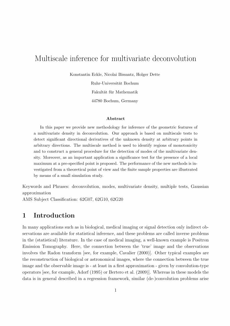
Figure 1: Example of a global map for monotonicity of a bivariate density.

This method allows for a global understanding of the shape of the density f . A particular

feature of the proposed method consists in the fact that by conducting formal statistical tests

the multiple level can be controlled (see Theorem 3.2).

For example, simultaneous tests for hypotheses of the form (2.2) and (2.3) can be used to

obtain a graphical representation of the local monotonicity behavior of the density as displayed

in Figure 1 for a bivariate density. The displayed map is based on tests for the hypotheses

(2.2) for a fixed scale h0 and different locations and directions (s1, t1), . . . , (sp, tp) (here taken

as the vertices of an equidistant grid and four equidistant directions on S1). Note that we

are investigating here a symmetric set of triples, that is, for every location tj both the triple

(sj, tj, h0) and (−sj, tj, h0) are considered. Thus, as Hsj ,tj ,h00,incr = H−s

j ,tj ,h00,decr , it is sufficient to

investigate only hypotheses of the form (2.2) in this setting. The figure shows the results of the

tests for the different hypotheses in (2.2). An arrow in a direction sj at a location tj represents

a rejection of the corresponding hypothesis Hsj ,tj ,h00,incr and provides therefore an indication of a

positive directional derivative of f in direction sj at the location tj. For a detailed description

of the settings used to provide Figure 1 and an analysis of the results we refer to Section 4.2.

If one is interested in specific shape constraints of the density, say in a test for a mode (local

maximum) at a given point x0, inference can be conducted investigating the hypotheses

Hsj ,tj ,h00,decr versus Hsj ,tj ,h0

1,decr (2.4)

for different pairs (t1, s1), . . . , (tp, sp), where t1, . . . , tp are points in a neighborhood of x0 on the

lines {x0 +λsj|λ > 0} (j = 1, . . . , p), respectively (of course, on could additionally use different

scales here).

4

Throughout this paper we will assume that all partial derivatives ∂sf of the density f are

uniformly bounded, such that the estimated quantity (2.1) is bounded by a constant which

does not depend on the triple (s, t, h). Using integration by parts, Plancherel’s identity and the

convolution theorem, we get

−∫Rd

∂sf(x)φt,h(x) dx =

∫Rd

f(x)∂sφt,h(x) dx (2.5)

=1

(2π)d

∫Rd

F (f)(y)F (∂sφt,h)(y) dy

=1

(2π)d

∫Rd

F (g)(y)

(F (∂sφt,h)

F (fε)

)(y) dy

=

∫Rd

g(x)F−1

(F (∂sφt,h)

F (fε)

)(x) dx.

Here,

F (f)(y) =

∫Rd

e−iy.xf(x) dx,

F−1(f)(x) =1

(2π)d

∫Rd

eix.yf(y) dy(x, y ∈ Rd

)denote the Fourier transform and its inverse, respectively, z is the complex conjugate of z ∈ Cand x.y stands for the standard inner product of x, y ∈ Rd.

For the construction of tests for the hypotheses in (2.2) and (2.3) we define the statistic

T ns,t,h =1

n

n∑i=1

Fs,t,h(Yi), (2.6)

where

Fs,t,h(Yi) = F−1(F (∂sφt,h)

F (fε)

)(Yi). (2.7)

Because (by (2.5))

E(T ns,t,h) = −∫Rd

∂sf(x)φt,h(x) dx,

it follows that T ns,t,h is a reasonable estimate of the quantity defined in (2.1), and hence the

statistics T ns,t,h define the main tool to study qualitative features of the density f . Inference on

local monotonicity of the density f will then be based on tests rejecting the hypotheses Hs,t,h0,incr

for small values of the corresponding statistic T ns,t,h and rejecting Hs,t,h0,decr for large values of T ns,t,h

for several directions s ∈ Sd−1, locations t ∈ [0, 1]d and scales h > 0. The multiple level of these

tests can be controlled by investigating the (asymptotic) maximum of appropriately normalized

statistics T ns,t,h calculated over a certain set of locations, directions and scales.

5

3 Asymptotic properties

In this section we investigate the asymptotic properties of a statistic which can be used to

control the multiple level of the tests introduced in Section 2. To be precise, we consider the

finite subset

Tn :={

(sj, tj, hj) | j = 1, . . . , p}⊆ Sd−1 × [0, 1]d × [hmin, hmax]

of cardinality p ≤ nK for the calculation of the maximum of appropriately standardized statistics

T ns,t,h, where K > 1 and for some ε > 0

hmin & n−1/d+ε and hmax = o((log(n) log log(n))−1). (3.1)

Throughout this paper we will make frequent use of multi-index notation, where α = (α1, . . . , αd) ∈Nd

0 denotes a multi-index (written in bold), |α| = α1 + . . .+αd its “length”, and for a sufficiently

smooth function f : Rd → R and a multi-index α we denote by

∂αf(x) =∂|α|

∂xα11 · . . . · ∂x

αdd

f(x)

its partial derivative.

Recall the definition of Fs,t,h in (2.7), to simplify the notation define for a point (sj, tj, hj) ∈ Tn

Fj = Fsj ,tj ,hj (3.2)

and consider the random variables

X(1)j =

√log(eh−dj )

log log(eeh−dj )

( hd/2+r+1j√ngn(tj)Vj

∣∣∣ n∑i=1

Fj(Yi)− nE(Fj(Y1))∣∣∣−√2 log(h−dj )

), (3.3)

where gn is a density estimator of g satisfying

‖g − gn‖∞ = o(log(n)−1) almost surely (3.4)

(for example a kernel density estimator as considered in Gine and Guillou (2002)) and

Vj = hd/2+r+1j ‖Fsj ,tj ,hj‖L2(Rd). (3.5)

The quantity Vj is well-defined under the assumptions presented below (see Lemma 5.2 for

details).

Note that the boundary of the hypotheses Hsj ,tj ,hj0,incr and H

sj ,tj ,hj0,decr in (2.2) and (2.3) is defined by∫

Rd ∂sjf(x)φtj ,hj(x) dx = 0 and in this case we have

1√nX

(1)j =

√log(eh−dj )

log log(eeh−dj )

( hd/2+r+1j√gn(tj)Vj

∣∣T nsj ,tj ,hj ∣∣−√

2 log(h−dj )√n

).

Consequently, we will investigate the asymptotic properties of max1≤j≤p X(1)j in the following

discussion. For this purpose we make the following assumptions.

6

Assumption 1. Assume that the density g is Lipschitz continuous and locally bounded from

below, i.e.

g(x) ≥ c > 0 for all x ∈ [0, 1]d.

Assumption 2. We assume a polynomial decay of the Fourier transform of the error density

fε, i.e. that there exist constants r > 0 for d ≥ 2 resp. r > 12

for d = 1 and 0 < Cu < Co such

that

Cu(1 + ‖y‖2

)−r/2 ≤ |F (fε)(y)| ≤ Co(1 + ‖y‖2

)−r/2.

Furthermore, let

d(d+1)/2e∑j=1

(1 + ‖y‖2)j/2∣∣∣ ∂j∂yjl

F (fε)(y)∣∣∣ ≤ Co(1 + ‖y‖2)−r/2

for all l = 1, . . . , d.

Note that as a direct consequence of Assumption 1 g is bounded from above and that there

exists a constant δ > 0 such that g(x) ≥ c2> 0 for all x ∈ [−δ, 1 + δ]d. Assumption 2 can be

seen as a multivariate generalization of the classical assumptions on the decay of the Fourier

transform of the error density in the ordinary smooth case (see e.g. Schmidt-Hieber et al.

(2013), Assumption 2). We also note that this assumption defines a mildly ill-posed situation

(see Bissantz and Holzmann (2008)). The next assumptions refer to the kernel φ and are

required for some technical arguments.

Assumption 3. Let ‖∂sφ‖L2(Rd) 6= 0 for all s ∈ Sd−1 and assume that ∂βφ exists in [−1, 1]d

and is continuous for all |β| ≤ dr+ 2e, where r is the constant from Assumption 2. We assume

further that for some δ > 0 the inequality∫Rd

(1 + ‖y‖2

)r+(d+δ)/2∣∣∣ ∂m∂yml

F (∂ekφ)(y)∣∣∣2 dy <∞

holds for all k, l = 1, . . . , d and m = 0, . . . , d(d+ 1)/2e, where ek, k = 1, . . . , d, denotes the kth

unit vector of Rd.

As ∣∣∣ ∂m∂yml

F (∂sφ)(y)∣∣∣2 =

∣∣∣ d∑k=1

sk∂m

∂ymlF (∂ekφ)(y)

∣∣∣2 ≤ C

d∑k=1

∣∣∣ ∂m∂yml

F (∂ekφ)(y)∣∣∣2

for all s ∈ Sd−1 and some constant C > 0 that only depends on d, Assumption 3 yields a

uniform upper bound for the integral∫Rd

(1 + ‖y‖2

)r+(d+δ)/2∣∣∣ ∂m∂yml

F (∂sφ)(y)∣∣∣2 dy

7

for all s ∈ Sd−1.

Recall the definition of X(1)j in (3.3) and define the vector X(1) = (X

(1)1 , . . . , X

(1)p )>. Our

first main result provides a uniform approximation of the probabilities P(X(1) ∈ A) by the

probabilities P(X ∈ A) for every half-open hyperrectangle A, where the components of the

vector X = (X1, . . . , Xp)> are defined by

Xj =

√log(eh−dj )

log log(eeh−dj )

(hd/2+r+1j

|∫Rd Fj(x) dBx|

Vj−√

2 log(h−dj ))

(3.6)

(j = 1, . . . , p), and (Bx)x∈Rd is a standard d-variate Brownian motion.

Theorem 3.1. Let A denote the set A := {(−∞, a1]× . . .× (−∞, ap] | a1, . . . , ap ∈ R}. Then,

supA∈A

∣∣P(X(1) ∈ A)− P

(X ∈ A

)∣∣ = o(1) for n→∞. (3.7)

Furthermore, the random variable max1≤j≤p Xj is almost surely bounded uniformly with respect

to n.

Theorem 3.1 will be used to control the multiple level of statistical tests for the hypotheses of

the form (2.2) and (2.3). To this end, let α ∈ (0, 1) and denote by κn(α) the smallest number

such that

P(

max1≤j≤p

Xj ≤ κn(α))≥ 1− α. (3.8)

By Theorem 3.1, κn(α) is bounded uniformly with respect to n and α. The jth hypothesis in

(2.2) is rejected, whenever

n−1

n∑i=1

Fj(Yi) < −κjn(α), (3.9)

where

κjn(α) =

√gn(tj)Vj√

nh−d/2−r−1j

( log log(eeh−dj )√log(eh−dj )

κn(α) +√

2 log(h−dj )). (3.10)

Similarly, the jth hypothesis in (2.3) is rejected, whenever

n−1

n∑i=1

Fj(Yi) > κjn(α). (3.11)

Theorem 3.2. Assume that the tests (3.9) and (3.11) for the hypotheses (2.2) and (2.3) are

performed simultaneously for j = 1, . . . , p. The probability of at least one false rejection of any

of the tests is asymptotically at most α, that is

P(∃j ∈ {1, . . . , p} : n−1|

n∑i=1

Fj(Yi)| > κjn(α))≤ α + o(1)

for n→∞.

8

Next we introduce a method for the detection and localization of the modes of the density. The

main idea is to conduct the local tests for modality proposed in (2.4) for a set of candidate

modes which does not assume any prior knowledge about the density. To be precise, we assume

the following condition on the set Tn: for any fixed h and s the set {t : (s, t, h) ∈ Tn} is

an equidistant grid in [0, 1]d with grid width h. Furthermore, for any fixed t and h the set

{s : (s, t, h) ∈ Tn} is a grid in Sd−1 with grid width converging to zero with increasing sample

size.

This grid is now used as follows to check if a point x0 ∈ (0, 1)d is a mode of f . Let T x0

n ⊂ Tn be

the set of all triples (s, t, h) ∈ Tn such that ch ≥ ‖x0− t‖ ≥ 2√dh for some c > 2

√d sufficiently

large and angle(x0 − t, s) → 0 for n → ∞. By the condition on Tn defined above, the set

T x0

n is nonempty for sufficiently large n. We now use the local tests (3.11) for the hypotheses

(2.4) and decide for a mode at the point x0 if the null hypotheses in (2.4) are rejected for all

triples in T x0

n . Note that by choosing the test locations as the vertices of an equidistant grid

no prior knowledge about the location of x0 has to be assumed. Theorem 3.3 below states that

the procedure detects all modes of the density with asymptotic probability one as n→∞.

Theorem 3.3. Let x0 ∈ (0, 1)d denote an arbitrary mode of the density f and assume that

there exist functions gx0 : Rd → R, fx0 : R→ R such that the density f has a representation of

the form

f(x) ≡ (1 + gx0(x))fx0(‖x− x0‖) (3.12)

(in a neighborhood of x0), gx0 is differentiable in a neighborhood of the point x0 such that

gx0(x) = o(1) and 〈∇gx0(x), e〉 = o(‖x − x0‖) if x → x0 for all e ∈ Rd with ‖e‖ = 1. In

addition, let fx0 be differentiable in a neighborhood of the point 0 with f ′x0(h) ≤ −ch(1 + o(1))

for h→ 0.

If the set {(s, t, h) ∈ Tn : h ≥ C log(n)1/(d+2r+4)n−1/(d+2r+4)

}for some C > 0 sufficiently large is nonempty, then the procedure described in the previous

paragraph detects the mode x0 with asymptotic probability one as n→∞.

The method to detect the modes of the density proposed in Theorem 3.3 proceeds in two steps:

the verification of the presence of a mode with asymptotic probability one in the asymptotic

regime presented above and its localization at the rate n−1/(d+2r+4) (up to some logarithmic

factor) given by the grid width.

4 Finite sample properties

In this section we illustrate the finite sample properties of the proposed multiscale inference.

The performance of the test for modality at a given point x0 (see the hypotheses in (2.4)) and

9

the dependence of its power on the bandwidth and the error variance is investigated. We also

illustrate how simultaneous tests for hypotheses of the form (2.2) and (2.3) can be used to

obtain a graphical representation of the local monotonicity properties of the density.

We consider two-dimensional densities, i.e. d = 2. The density fε of the errors in model (1.1) is

given by a symmetric bivariate Laplacian with scale parameter σ > 0 which is defined through

its characteristic function

F (fε)(y1, y2) =1

1 + 12σ2(y2

1 + y22)

(4.1)

for (y1, y2) ∈ R2 (cf. Kotz et al. (2001), Chapter 5). This means that r = 2 and straightforward

calculations show that

Fs,t,h(x1, x2) = F−1(

F (∂sφt,h)

F (fε)

)(x1, x2) =

(∂s −

σ2

2

(∂2e1∂s + ∂2

e2∂s))φt,h(x1, x2) (4.2)

for (x1, x2) ∈ R2. The test function is chosen as

φ(x1, x2) = c2(1− x41)(1− x4

2)1{|x1| ≤ 1, |x2| ≤ 1

},

where c2 defines the normalization constant, that is

c2 =∥∥(1− x4

1)(1− x42)1{|x1| ≤ 1, |x2| ≤ 1

}∥∥−1

L1(Rd)

(note that φ is smooth within its support). Moreover, the integration by parts formula gives

−∫R2

∂sf(x)φt,h(x) dx =

∫R2

f(x)∂sφt,h(x) dx

as φ vanishes on the boundary of its support. Finally, by the representation (4.2) we find that

the deconvolution kernel possesses all properties that are used for the proof of Theorem 3.1 and

therefore Theorem 3.1 is also satisfied for the function φ.

Throughout this section the nominal level is fixed as α = 0.05.

4.1 A local test for modality

In this section we investigate the performance of a local test for the existence of a mode

(more precisely a local maximum) at a given location x0 which is defined by testing several

hypotheses of the form (2.4) simultaneously. Moreover, the influence of the choice of the

different parameters on the power of the test is also investigated. To be precise, we conduct

four tests for the hypotheses (2.4) with a fixed bandwidth h = h0. The postulated mode is given

by the point x0 = (0, 0)> and the four directions and locations are chosen as s1 = t1 = (1, 0)>,

10

Figure 2: Illustration of the four local tests for monotonicity used to define the test (4.3) for

h0 = 0.5. The crosshatched squares display the support of the functions Fsj ,tj ,h0, j = 1, . . . , 4,

and the arrows the directional vectors sj, j = 1, . . . , 4.

s2 = t2 = (0, 1)>, s3 = t3 = (−1, 0)> and s4 = t4 = (0,−1)>. We conclude that f has a local

maximum at the point x0 = (0, 0)>, whenever all hypotheses

Hsj ,tj ,h00,decr , j = 1, . . . , 4,

are rejected, that is

T nsj ,tj ,h0 > κjn(α) for all j = 1, . . . , 4, (4.3)

where κjn(α) is defined by (3.10). An illustration of the considered situation is provided in

Figure 2. The quantiles κn(0.05) defined in (3.8) are derived by 1000 simulation runs based on

normal distributed random vectors. In Table 1 we display the normalized quantiles√nκ1

n(0.05)

for the sample sizes n = 500, 1000, 4000 observations and h0 = 0.5. Here, the value of the

parameter of the Laplacian error density has been chosen as σ = 0.075.

n√nκ1

n(0.05)

500 0.039

1000 0.044

4000 0.041

Table 1: Simulated quantiles√nκ1

n(0.05) of the test (4.3). The density fε is defined in (4.1).

The approximation of the level of the test for a mode at the point x0 defined by (4.3) is

investigated using a uniform distribution on the square [−2.5, 2.5]2 for the density f . For power

considerations we sample the Zi in model (1.1) from a standard normal distribution. The

results are displayed in the left part of Table 2. By its construction, the multiscale method is

11

rather conservative but nevertheless it is able to detect the mode with increasing sample size.

In order to obtain a better approximation of the nominal level we propose a calibrated version

of the test, where the quantiles are chosen such that the test keeps its nominal level α = 0.05.

Note that this calibration does not require any knowledge about the unknown density f . The

simulated rejection probabilities are presented in the right part of Table 2 for the parameters

h0 = 0.5 and σ = 0.075. We find that the calibrated test performs very well.

n level power level (cal.) power (cal.)

500 0.3 39.4 4.2 74.7

1000 0.1 71.1 4.0 93.3

4000 0.4 99.9 3.1 100

Table 2: Simulated level and power of the test (4.3) for a mode at the point x0 = (0, 0)> of a 2-

dimensional density. The random variables Zi in model (1.1) are standard normal distributed.

Second and third column: test defined by (4.3); fourth and fifth column: test defined by (4.3),

where the quantiles κjn(α) are replaced by calibrated quantiles.

Next we fix the number of observations, that is n = 1000, the value of the parameter σ = 0.075

and vary the bandwidth h0 to investigate its influence on the power of the test (4.3). Recall

that by the proposed choice of a Laplacian error density, the deconvolution kernel has compact

support in [−1, 1]2. Hence, by dividing the bandwidth by 2 a fourth of the area is considered

and (roughly) a fourth of the number of observations is used for the local test. Thus, we observe

a decrease in power of the test for decreasing values of bandwidths which is illustrated in Table

3.

h0 level power level (cal.) power (cal.)

0.3 0.5 7.8 4.6 35.3

0.4 0.2 29.6 4.5 71.7

0.5 0.1 71.7 4.0 93.3

0.6 0.2 95.3 4.8 99.5

Table 3: Dependence of the power of the test (4.3) for a mode at the point x0 = (0, 0)> on the

bandwidth in the situation of Table 2 where the number of observations is fixed to n = 1000.

Second and third column: test defined by (4.3); fourth and fifth column: test defined by (4.3),

where the quantiles κjn(α) are replaced by calibrated quantiles.

We also investigate the influence of the scale parameter σ on the power of the test (4.3). To

this end, we fix the bandwidth as h0 = 0.5 and the number of observations as n = 1000 and

vary the value of σ. The results are shown in Table 4 and we observe that an increase in the

12

value of σ decreases the power of the test. On the other hand the power of the tests is very

stable for small values of σ.

σ level power level (cal.) power (cal.)

0.0 (direct setting) 0.4 77.7 4.7 94.1

0.075 0.1 71.7 4.0 93.3

0.15 0.2 71.1 3.6 92.8

0.3 0.4 62.3 3.8 87.2

1.0 0.3 31.4 4.5 59.4

Table 4: Dependence of the power of the test (4.3) for a mode at the point x0 = (0, 0)> on

the scale parameter in the situation considered in Table 2 where the number of observations is

fixed to n = 1000. Second and third column: test defined by (4.3); fourth and fifth column: test

defined by (4.3), where the quantiles κjn(α) are replaced by calibrated quantiles.

Next we investigate the influence of the shape of the modal region on the power of the test

(4.3). To this end, we fix the values of h0 = 0.5 and σ = 0.075 and use normal distributed

random variables Zi with mean zero and non-diagonal covariance matrices

Σ1 =(

0 0.5−1 1.5

)and Σ2 =

(−0.5 1−2 2.5

). (4.4)

The simulated rejection probabilities are presented in Table 5 and show that the absolute values

of the eigenvalues of the covariance matrix have an influence on the power of the test. In the case

of N (0,Σ1)-distributed random variables Zi (eigenvalues 0.5 and 1) the test performs better as

for standard normal observations (with both eigenvalues equal to one). In the case of N (0,Σ2)-

distributed random variables Zi (eigenvalues 0.5 and 1.5) the test performs slightly worse than

in the first case but still better as for standard normal observations due to the eigenvalue with

absolute value smaller than one. We note again the superiority of the calibrated test.

We also investigate the influence of a (slight) misspecification of the position of the candidate

mode on the power of the test (4.3) in the situation considered in Table 2 with candidate mode

x0 = (0.2, 0.2)>. The results are presented in Table 6. We find that the slight misspecification

of the position of the candidate mode affects the power of the method only slightly.

Finally we consider a bimodal density and conduct simultaneously local tests for modality based

on the hypotheses (2.4) for the candidate modes x1 = (0, 0)> and x2 = (3, 0)>. We conduct eight

tests for the hypotheses (2.4) for a fixed bandwidth h = h0 = 0.5 with s1 = s5 = t1 = (1, 0)>,

s2 = s6 = t2 = (0, 1)>, s3 = s7 = t3 = (−1, 0)>, s4 = s8 = t4 = (0,−1)> and t5 = (4, 0)>,

t6 = (3, 1)>, t7 = (2, 0)>, t8 = (3,−1)> and conclude that f has a local maximum in x1 = (0, 0)>

13

Σ1 Σ2

n power power (cal.) power power (cal.)

500 78.5 94.7 72.6 92.6

1000 96.7 99.3 96.5 98.9

4000 100 100 100 100

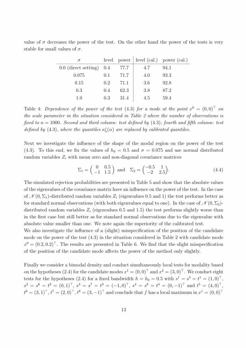
Table 5: Dependence of the power of the test (4.3) for a mode at the point x0 = (0, 0)> on

the shape of the modal region. The random variables Zi are centered normal distributed with

covariance matrices Σ1 and Σ2 given in (4.4). Second and fourth column: test defined by (4.3);

third and fifth column: test defined by (4.3), where the quantiles κjn(α) are replaced by calibrated

quantiles.

x0 = (0.2, 0.2)>

n power power (cal.)

500 34.9 70.8

1000 70.1 89.3

4000 99.9 100

Table 6: Influence of a misspecification of the mode on the power of the test (4.3) for a mode

at the point x0 = (0.2, 0.2)>. The random variables Zi in model (1.1) are standard normal

distributed and therefore the true mode is given by (0, 0)>. Second column: test defined by

(4.3); third column: test defined by (4.3), where the quantiles κjn(α) are replaced by calibrated

quantiles.

whenever all hypotheses

Hsj ,tj ,h00,decr , j = 1, . . . , 4,

are rejected, that is

T nsj ,tj ,h0 > κjn(α) for all j = 1, . . . , 4 (4.5)

and that f has a local maximum in x2 = (3, 0)> whenever all hypotheses

Hsj ,tj ,h00,decr , j = 5, . . . , 8,

are rejected, that is

T nsj ,tj ,h0 > κjn(α) for all j = 5, . . . , 8, (4.6)

where the quantile κjn(α) is defined by (3.10). An illustration of the considered scales is provided

in Figure 3. For the investigation of the approximation of the nominal level we consider a

uniform distribution on the rectangle [−2.5, 5.5]×[−2.5, 2.5] for the density f . The scaling factor

in the Laplace density is given by σ = 0.075. For power investigations we consider two bimodal

densities given by a uniform mixture of a standard normal distribution and a N ((3, 0)>, I)

14

Figure 3: Illustration of the eight local tests for monotonicity used to create the tests (4.5) and

(4.6). The crosshatched squares display the support of the functions Fsj ,tj ,h0, j = 1, . . . , 8, and

the arrows the directional vectors sj, j = 1, . . . , 8.

distribution (symmetric) and a uniform mixture of a N ((0.0)>, 1.2I) and a N ((3.2, 0.1)>, 0.8I)

distribution (asymmetric). The results for the calibrated version of the test are given in Table

7.

Symmetric Asymmetric

n level power x1 power x2 power x1 power x2

500 5.3 34.6 33.0 23.6 48.5

1000 5.2 48.7 49.9 39.0 72.9

4000 4.2 84.4 81.7 76.1 97.1

Table 7: Simulated level and power of the tests (4.5) and (4.6) for a mode at the points

x1 = (0, 0)> and x2 = (3, 0)>, where the quantiles κjn(α) are replaced by calibrated quan-

tiles. The random variables Zi in model (1.1) are given by a uniform mixture of a standard

normal distribution and a N ((3, 0)>, I) distribution (symmetric) and a uniform mixture of a

N ((0.0)>, 1.2I) and a N ((3.2, 0.1)>, 0.8I) distribution (asymmetric).

We observe that in the symmetric case the test detects both modes with (roughly) the same

power, whereas in the asymmetric case the mode with smaller variance (even though there is a

slight misspecification of its position) is detected more often.

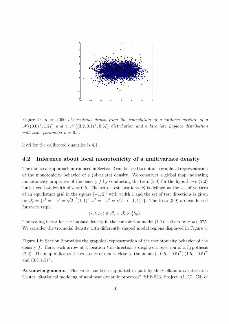
A scatter plot of n = 4000 observations from the convolution of the asymmetric bimodal density

and a bivariate Laplace distribution with scale parameter σ = 0.5 is given in Figure 4. Here,

a look at the scatter plot does not give a hint on the number of modes of the distribution.

However, the test (4.5), where the quantiles κjn(α) are replaced by calibrated quantiles, is still

able to detect a mode at (0, 0)> in 48.4 percent of the repetitions and the test (4.6) with

calibrated quantiles detects a mode in (3, 0)> in 81.4 percent of the repetitions. The simulated

15

Figure 4: n = 4000 observations drawn from the convolution of a uniform mixture of a

N ((0.0)>, 1.2I) and a N ((3.2, 0.1)>, 0.8I) distribution and a bivariate Laplace distribution

with scale parameter σ = 0.5.

level for the calibrated quantiles is 4.1.

4.2 Inference about local monotonicity of a multivariate density

The multiscale approach introduced in Section 2 can be used to obtain a graphical representation

of the monotonicity behavior of a (bivariate) density. We construct a global map indicating

monotonicity properties of the density f by conducting the tests (3.9) for the hypotheses (2.2)

for a fixed bandwidth of h = 0.5. The set of test locations Tt is defined as the set of vertices

of an equidistant grid in the square [−1, 2]2 with width 1 and the set of test directions is given

by Ts = {s1 = −s3 =√

2−1

(1, 1)>, s2 = −s4 =√

2−1

(−1, 1)>}. The tests (3.9) are conducted

for every triple

(s, t, h0) ∈ Ts ×Tt × {h0}.

The scaling factor for the Laplace density in the convolution model (1.1) is given by σ = 0.075.

We consider the tri-modal density with differently shaped modal regions displayed in Figure 5.

Figure 1 in Section 2 provides the graphical representation of the monotonicity behavior of the

density f . Here, each arrow at a location t in direction s displays a rejection of a hypothesis

(2.2). The map indicates the existence of modes close to the points (−0.5,−0.5)>, (1.5,−0.5)>

and (0.5, 1.5)>.

Acknowledgements. This work has been supported in part by the Collaborative Research

Center “Statistical modeling of nonlinear dynamic processes” (SFB 823, Project A1, C1, C4) of

16

Figure 5: The density of a (uniform) mixture of a N ((−0.4,−0.57)>, 0.2I),

N ((1.5,−0.6)>, 0.25I) and N ((0.45, 1.6)>, 0.5I) distribution.

the German Research Foundation (DFG). The authors would like to thank Martina Stein, who

typed parts of this manuscript with considerable technical expertise.

References

Adler, R. and Taylor, J. (2007). Random Fields and Geometry. Springer Monographs in Mathematics.

Springer New York.

Adorf, H. M. (1995). Hubble space telescope image restoration in its fourth year. Inverse Problems,

11(4):639.

Balabdaoui, F., Bissantz, K., Bissantz, N., and Holzmann, H. (2010). Demonstrating single and multi-

ple currents through the e. coli-SecYEG-pore: testing for the number of modes of noisy observations.

J. Amer. Statist. Assoc., 105(489):136–146.

Bertero, M., Boccacci, P., Desidera, G., and Vicidomini, G. (2009). Image deblurring with Poisson

data: from cells to galaxies. Inverse Problems, 25(12):123006, 26.

Bissantz, N., Dumbgen, L., Holzmann, H., and Munk, A. (2007). Non-parametric confidence bands in

deconvolution density estimation. J. Roy. Statist. Soc. Ser. B, 69(3):483–506.

Bissantz, N. and Holzmann, H. (2008). Statistical inference for inverse problems. Inverse Problems,

24(3):034009, 17.

Butucea, C. and Matias, C. (2005). Minimax estimation of the noise level and of the deconvolution

density in a semiparametric convolution model. Bernoulli, 11(2):309–340.

17

Carroll, R. J. and Hall, P. (1988). Optimal rates of convergence for deconvolving a density. J. Amer.

Statist. Assoc., 83(404):1184–1186.

Cavalier, L. (2000). Efficient estimation of a density in a problem of tomography. Ann. Statist.,

28(2):630–647.

Chernozhukov, V., Chetverikov, D., and Kato, K. (2016). Central limit theorems and bootstrap in

high dimensions. Preprint, arXiv:1412.3661.

Comte, F. and Lacour, C. (2013). Anisotropic adaptive kernel deconvolution. Ann. Inst. Henri

Poincare Probab. Stat., 49(2):569–609.

Diggle, P. J. and Hall, P. (1993). A Fourier approach to nonparametric deconvolution of a density

estimate. J. Roy. Statist. Soc. Ser. B, 55(2):523–531.

Dumbgen, L. and Spokoiny, V. G. (2001). Multiscale testing of qualitative hypotheses. Ann. Statist.,

29(1):124–152.

Eckle, K., Bissantz, N., Dette, H., Proksch, K., and Einecke, S. (2016). Multiscale inference for a

multivariate density with applications to x-ray astronomy. Preprint, arXiv:1412.3661.

Fan, J. (1991). On the optimal rates of convergence for nonparametric deconvolution problems. Ann.

Statist., 19(3):1257–1272.

Gine, E. and Guillou, A. (2002). Rates of strong uniform consistency for multivariate kernel density

estimators. Ann. Inst. H. Poincare Probab. Statist., 38(6):907–921. En l’honneur de J. Bretagnolle,

D. Dacunha-Castelle, I. Ibragimov.

Grund, B. and Hall, P. (1995). On the minimisation of Lp error in mode estimation. Annals of

Statistics, 23:2264–2284.

Holzmann, H., Bissantz, N., and Munk, A. (2007). Density testing in a contaminated sample. J.

Multivariate Anal., 98(1):57–75.

Khoshnevisan, D. (2002). Multiparameter Processes: An Introduction to Random Fields. Monographs

in Mathematics. Springer.

Kotz, S., Kozubowski, T. J., and Podgorski, K. (2001). Symmetric Multivariate Laplace Distribution.

Birkhauser Boston, Boston, MA.

Meister, A. (2009). On testing for local monotonicity in deconvolution problems. Statist. Probab. Lett.,

79(3):312–319.

Pensky, M. and Vidakovic, B. (1999). Adaptive wavelet estimator for nonparametric density decon-

volution. Ann. Statist., 27(6):2033–2053.

Romano, J. (1988). On weak convergence and optimality of kernel density estimates of the mode.

Annals of Statistics, 16:629–647.

Sarkar, A., Pati, D., Mallick, B. K., and Carroll, R. J. (2015). Bayesian semiparametric multivariate

density deconvolution. Preprint, arXiv:1404.6462.

Schmidt-Hieber, J., Munk, A., and Dumbgen, L. (2013). Multiscale methods for shape constraints in

deconvolution: confidence statements for qualitative features. Ann. Statist., 41(3):1299–1328.

van Es, B., Jongbloed, G., and van Zuijlen, M. (1998). Isotonic inverse estimators for nonparametric

deconvolution. Ann. Statist., 26(6):2395–2406.

18

5 Proof of Theorem 3.1

We split the proof of Theorem 3.1 in three parts. The first part is dedicated to several auxiliary

results involving the deconvolution kernel Fs,t,h. In the second part of the proof we show the

approximation (3.7). Finally we conclude by proving the boundedness of the limit distribution

in the third part.

Throughout this section the symbols . and & mean less or equal and greater or equal, res-

pectively, up to a multiplicative constant independent of n and (s, t, h), and the symbol |as,t,h| �|bs,t,h| means that |as,t,h/bs,t,h| is bounded from above and below by positive constants.

5.1 Auxiliary results

We begin with some basic transformations of the deconvolution kernel Fs,t,h. Recall that

Fs,t,h(.) = F−1(F (∂sφt,h)

F (fε)

)(.) = h−d−1F−1

(∫Rd e

−iy.x(∂sφ)((x− t)/h) dx

F (fε)(y)

)(.)

by definition of the kernel φt,h and the Fourier transform. A substitution in the inner integral

shows that

Fs,t,h(.) = h−1F−1(e−iy.tF (∂sφ)(hy)

F (fε)(y)

)(.). (5.1)

By the definition of the inverse Fourier transform and a substitution in the outer integral, we

obtain

Fs,t,h(x) =h−1

(2π)d

∫Rd

eix.ye−iy.tF (∂sφ)(hy)

F (fε)(y)dy =

h−d−1

(2π)d

∫Rd

eiy.x−th

F (∂sφ)(y)

F (fε)(y/h)dy. (5.2)

Furthermore, as ∂sφ =∑d

k=1 sk∂ekφ, where ek, k = 1, . . . , d, denotes the kth unit vector of Rd,

we have

F (∂sφ)(y) =d∑

k=1

skiykF (φ)(y),

where i denotes the imaginary unit. The following lemma presents some immediate conse-

quences of the Assumptions 2 and 3 made in Section 3.

Lemma 5.1. Let l ∈ {1, . . . , d}, m ≥ 2 and m = d(d+ 1)/me. It holds

(i) Ss =

∫Rd

(1 + ‖y‖2

)r/2∣∣F (∂sφ)(y)∣∣ dy <∞ uniformly with respect to s;

(ii)

∫Rd

∣∣∣ ∂m∂yml

( F (∂sφ)(y)

F (fε)(y/h)

)∣∣∣ dy . h−r.

19

Proof of Lemma 5.1:

(i): An application of Cauchy-Schwartz’s inequality yields for any δ > 0

Ss =

∫Rd

(1 + ‖y‖2

)r/2+(d+δ)/4(1 + ‖y‖2

)−(d+δ)/4∣∣F (∂sφ)(y)∣∣ dy

≤(∫

Rd

(1 + ‖y‖2

)r+(d+δ)/2∣∣F (∂sφ)(y)∣∣2 dy

)1/2∥∥(1 + ‖y‖2)−(d+δ)/4∥∥

L2(Rd).

By Assumption 3, there exists a constant δ > 0 such that the latter integral is bounded uni-

formly with respect to s. Hence, the assertion follows from the integrability of the function

(1 + ‖y‖2)−(d+δ)/2.

(ii): By Leibniz’s rule we have

∣∣∣ ∂m∂yml

( F (∂sφ)(y)

F (fε)(y/h)

)∣∣∣ . m∑k=0

∣∣∣ ∂m−k∂ym−kl

F (∂sφ)(y)∂k

∂ykl

1

F (fε)(y/h)

∣∣∣.Moreover, from Lemma 7.2 it follows that∣∣∣ ∂k

∂ykl

1

F (fε)(y/h)

∣∣∣ . ∑(m1,...,mk)∈Mk

1

|F (fε)(y/h)|m1+...+mk+1h−k

k∏j=1

∣∣∣( ∂j∂yjl

F (fε))

(y/h)∣∣∣mj

,

where Mk is the set of all k-tuples of non-negative integers satisfying∑k

j=1 jmj = k. Assump-

tion 2 in Section 3 yields the estimates∣∣∣ ∂j∂yjl

F (fε)(y)∣∣∣ . (1 + ‖y‖2

)−(r+j)/2and

1

|F (fε)(y)|.(1 + ‖y‖2

)r/2.

Thus, as∑k

j=1 jmj = k for some (m1, . . . ,mk) ∈Mk, we find

∣∣∣ ∂k∂ykl

1

F (fε)(y/h)

∣∣∣ . h−k∑

(m1,...,mk)∈Mk

(1 + ‖ y

h‖2)(m1+...+mk+1)r/2

k∏j=1

(1 + ‖ y

h‖2)−mj(r+j)/2

. h−k∑

(m1,...,mk)∈Mk

(1 + ‖ y

h‖2)(m1+...+mk+1)r/2(

1 + ‖ yh‖2)−(m1+...+mk)r/2−k/2

. h−k(1 + ‖ y

h‖2)(r−k)/2

.

Hence, ∣∣∣ ∂m∂yml

( F (∂sφ)(y)

F (fε)(y/h)

)∣∣∣ . m∑k=0

h−k∣∣∣ ∂m−k∂ym−kl

F (∂sφ)(y)∣∣∣(1 + ‖ y

h‖2)(r−k)/2

.

In the case r ≥ k, the claim is now a direct consequence of the estimate

h−k(1 + ‖ y

h‖2)(r−k)/2

. h−r(1 + ‖y‖2)(r−k)/2,

20

similar arguments as given in proof of (i) and Assumption 3.

If r < k we divide the integration area into the ball B1(0) and its complement. For the integral

h−k∫B1(0)C

∣∣∣ ∂m−k∂ym−kl

F (∂sφ)(y)∣∣∣(1 + ‖ y

h‖2)(r−k)/2

dy

we have h−k(1+‖ y

h‖2)(r−k)/2

. h−r. Therefore, we can bound the integral over the complement

of the unit ball by the integral over Rd and proceed similarly to the first case. It remains to

consider the integral over the ball B1(0). To this end, notice that

h−k(1 + ‖ y

h‖2)(r−k)/2 ≤ h−r‖y‖r−k.

Hence, by the boundedness of ∂m−k

∂ym−kl

F (∂sφ) (which follows from the compactness of the support

of φ) it remains to show that the integral∫B1(0)

‖y‖r−k dy .∫ 1

0

ρd−1+r−k dρ

is bounded, where we used a polar coordinate transform to obtain the inequality. As k ≤d(d+ 1)/2e and r > 0, the integral on the right hand side is obviously finite.

Part (i) of the following lemma shows that the constants V1, . . . , Vp defined in (3.5) are uniformly

bounded from above and below.

Lemma 5.2. It holds

(i) ‖Fs,t,h‖L2(Rd) � h−d/2−r−1;

(ii)∥∥Fs,t,h‖x− t‖∥∥L2(Rd)

. h−d/2−r;

(iii) ‖Fs,t,hFs′,t′,h′‖L1(Rd) . (hh′)−d/2−r−1;

(iv)∥∥Fs,t,hFs′,t′,h′‖x− t‖‖x− t′‖∥∥L1(Rd)

. (hh′)−d/2−r.

Proof of Lemma 5.2:

(i): Using Plancherel’s theorem and the representation (5.1), we obtain

‖Fs,t,h‖2L2(Rd) � h−2

∥∥∥e−iy.tF (∂sφ)(h.)

F (fε)(.)

∥∥∥2

L2(Rd)= h−2

∫Rd

∣∣∣F (∂sφ)(hy)

F (fε)(y)

∣∣∣2 dy. (5.3)

It now follows from Assumption 2 and a substitution that

‖Fs,t,h‖2L2(Rd) . h−d−2r−2

∫Rd

(1 + ‖y‖2)r

∣∣F (∂sφ)(y)∣∣2 dy,

21

and the latter integral is bounded by Assumption 3 which concludes the proof of the upper

bound.

For the lower bound we find from (5.3) and Assumption 2 that

‖Fs,t,h‖2L2(Rd) & h−2

∫Rd

(1 + ‖y‖2

)r∣∣F (∂sφ)(hy)∣∣2 dy

& h−d−2

∫Rd

(1 + ‖ y

h‖2)r∣∣F (∂sφ)(y)

∣∣2 dy & h−d−2r−2

∫Ba(0)C

∣∣F (∂sφ)(y)∣∣2 dy

for any constant a > 0. Moreover,∫Ba(0)C

∣∣F (∂sφ)(y)∣∣2 dy =

∫Rd

∣∣F (∂sφ)(y)∣∣2 dy −

∫Ba(0)

∣∣F (∂sφ)(y)∣∣2 dy & ‖∂sφ‖2

L2(Rd)

for a sufficiently small radius a by the integrability of |F (∂sφ)|2 (Assumption 3) and Plancherel’s

theorem. Furthermore, the mapping s 7→ ‖∂sφ‖L2(Rd) is continuous such that by Assumption 3

‖∂sφ‖L2(Rd) ≥ c > 0 for a constant c that does not depend on s.

(ii): The representation (5.2) and a substitution in the integral for the variable x show

∥∥Fs,t,h‖x− t‖∥∥2

L2(Rd)=

h−d

(2π)2d

∫Rd

‖x‖2∣∣∣ ∫

Rd

eiy.xF (∂sφ)(y)

F (fε)(y/h)dy∣∣∣2 dx.

As ‖x‖2 = x21 + . . .+ x2

d, the differentiation rule for Fourier transforms yields

∥∥Fs,t,h‖x− t‖∥∥2

L2(Rd)=

h−d

(2π)2d

d∑k=1

∫Rd

∣∣∣ ∫Rd

eiy.x∂

∂yk

( F (∂sφ)(y)

F (fε)(y/h)

)dy∣∣∣2 dx

= h−dd∑

k=1

∥∥∥F−1( ∂

∂yk

( F (∂sφ)(y)

F (fε)(y/h)

))∥∥∥2

L2(Rd)

� h−dd∑

k=1

∥∥∥ ∂

∂yk

( F (∂sφ)(y)

F (fε)(y/h)

)∥∥∥2

L2(Rd),

where the last identity follows from Plancherel’s theorem. We now proceed similarly as in the

proof of Lemma 5.1 (ii) and note that

∂

∂yk

F (∂sφ)(y)

F (fε)(y/h)=

∂

∂ykF (∂sφ)(y)

1

F (fε)(y/h)− F (∂sφ)(y)(

F (fε)(y/h))2

∂

∂yk

(F (fε)(y/h)

).

An application of the Assumptions 2 and 3 shows∥∥∥ ∂

∂ykF (∂sφ)(y)

1

F (fε)(y/h)

∥∥∥2

L2(Rd). h−2r

∫Rd

∣∣∣ ∂∂yk

F (∂sφ)(y)∣∣∣2(1 + ‖y‖2

)rdy . h−2r.

22

Moreover, by Assumption 2, we have∥∥∥ F (∂sφ)(y)(F (fε)(y/h)

)2

∂

∂yk

(F (fε)(y/h)

)∥∥∥2

L2(Rd). h−2

∫Rd

∣∣F (∂sφ)(y)∣∣2(1 + ‖ y

h‖2)r−1

dy.

This concludes the proof for r ≥ 1. For r < 1 we split up the area of integration into the ball

B1(0) and its complement and find the required result for the integration over the complement

using similar arguments as in the proof of Lemma 5.1 (ii). For the integral over the unit ball

we also follow the line of arguments presented in the proof of Lemma 5.1 (ii) which yields the

required result provided that the integral on the right hand side of the inequality∫B1(0)

‖y‖2r−2 dy .∫ 1

0

ρd−1+2r−2 dρ

exists. This is the case for all r > 0 if d ≥ 2 and all r > 12

in the case d = 1.

(iii) and (iv): These are direct consequences of Holder’s inequality and (i) resp. (ii).

The following Lemma will be used in the second part of the proof of Theorem 3.1.

Lemma 5.3. For 1 ≤ j, k ≤ p and m ≥ 2 we have for the function Fj = Fsj ,tj ,hj defined in

(3.2)

(i) |Fj(x)| . h−d−r−1j for all x ∈ Rd;

(ii) E(|Fj(Y1)|m) . h−(m−1)d−mr−mj .

Proof of Lemma 5.3:

(i): Using the representation (5.2) and Assumption 2 it follows that

|Fj(x)| . h−d−1j

∫Rd

∣∣∣ F (∂sjφ)(y)

F (fε)(y/hj)

∣∣∣ dy . h−d−r−1j

∫Rd

(1+‖y‖2

)r/2∣∣F (∂sjφ)(y)∣∣ dy = h−d−r−1

j Ssj .

The claim follows from the uniform boundedness of Ssj shown in Lemma 5.1 (i).

(ii): Using the representation (5.2), the boundedness of the density g and a substitution we get∫Rd

∣∣Fj(x)∣∣mg(x) dx . h−md−mj

∫Rd

∣∣∣ ∫Rd

eiy.x−tj

hjF (∂sjφ)(y)

F (fε)(y/hj)dy∣∣∣m dx

= h−(m−1)d−mj

∫Rd

∣∣∣ ∫Rd

eix.yF (∂sjφ)(y)

F (fε)(y/hj)dy∣∣∣m dx.

23

The proof will be completed showing the estimate∫Rd

∣∣∣ ∫Rd

eix.yF (∂sjφ)(y)

F (fε)(y/hj)dy∣∣∣m dx . h−mrj .

For this purpose we decompose the domain of integration for the variable x in two parts: the

cube [−δ, δ]d for some δ > 0 and its complement. For the integral with respect to the cube

we use the upper bound∫Rd

∣∣ F (∂sjφ)(y)

F (fε)(y/hj)

∣∣ dy . h−rj provided in the proof of (i) which yields the

required result.

For the integral with respect to ([−δ, δ]d)C note that∫([−δ,δ]d)C

∣∣∣ ∫Rd

eix.yF (∂sjφ)(y)

F (fε)(y/hj)dy∣∣∣m dx ≤

d∑k=1

d∑l=1

∫Ak,l

∣∣∣ ∫Rd

eix.yF (∂sjφ)(y)

F (fε)(y/hj)dy∣∣∣m dx ,

where the sets Ak,l are defined by

Ak,l ={x ∈ Rd | |xk| > δ, |xl| ≥ |xl′| for all l′ 6= l

}.

Now m = d(d+ 1)/me fold integration by parts yields∣∣∣ ∫Rd

eix.yF (∂sjφ)(y)

F (fε)(y/hj)dy∣∣∣m =

1

|xl|mm∣∣∣ ∫

Rd

eix.y∂m

∂yml

( F (∂sjφ)(y)

F (fε)(y/hj)

)dy∣∣∣m,

provided that ∂m

∂yml

( F (∂sjφ)(y)

F (fε)(y/hj)

)∈ L1(Rd), which holds by Lemma 5.1 (ii). A further application

of Lemma 5.1 (ii) shows that∫Ak,l

∣∣∣ ∫Rd

eix.yF (∂sjφ)(y)

F (fε)(y/hj)dy∣∣∣m dx . h−mrj

∫[−δ,δ]C

|xl|d−1

|xl|d+1dxl,

as |xl′| ≤ |xl| for all l′ 6= l and |xl| > δ in Ak,l.

5.2 Proof of the approximation (3.7)

For the consideration of the absolute values we introduce the set

T ′n := Tn ∪ {(−s, t, h) | (s, t, h) ∈ Tn} =: {(sj, tj, hj) | j = 1, . . . , 2p}

and denote by A ′ the set of all hyperrectangles in R2p of the form

A = {w ∈ R2p | aj ≤ wj ≤ bj for all 1 ≤ j ≤ 2p}

for some −∞ ≤ aj ≤ bj ≤ ∞ (1 ≤ j ≤ 2p).

24

We will show below in Section 5.2.1 that the random vectors Xi = (Xi,1, . . . , Xi,2p)> ∈ R2p,

i = 1, . . . , n, with

Xi,j = hd/2+r+1j

(Fj(Yi)− E(Fj(Y1))

)(i = 1, . . . , n, j = 1, . . . , 2p)

fulfill

supA∈A ′

∣∣∣P( 1√n

n∑i=1

Xi ∈ A)− P

( 1√n

n∑i=1

Y ′i ∈ A)∣∣∣ . (h−dmin log7(n)

n

)1/6

+(h−dmin log3(n)

n1−2/q

)1/3

(5.4)

for any q > 0, where Y ′1 , . . . , Y′n are independent random vectors, Y ′i = (Y ′i,1, . . . , Y

′i,2p)

> ∼N (0,E(XiX

>i )), i = 1, . . . , n. Note that we have

1√n

n∑i=1

Y ′i ∼ N(0,E(X1X>1 )),

where

E(X1X>1 ) =

((hjhk)

d/2+r+1(E(Fj(Y1)Fk(Y1))− E(Fj(Y1))E(Fk(Y1))

))1≤j,k≤2p

,

as the random variables X1, . . . , Xn are i.i.d. and Y ′1 , . . . , Y′n are independent.

Introduce a Gaussian process (B(Φ))Φ∈L∞(Rd) indexed by L∞(Rd) as a process whose mean and

covariance functions are 0 and∫Rd

Φ1(x)Φ2(x)g(x) dx−∫Rd

Φ1(x)g(x) dx

∫Rd

Φ2(x)g(x) dx, (5.5)

respectively. Hence, there exists a version of B(Φ) such that

1√n

n∑i=1

Y ′i =(hd/2+r+11 B(F1), . . . , h

d/2+r+12p B(F2p)

)>.

To derive an alternative representation of the process B recall the definition of the isonormal

process (B(Φ))Φ∈L2(Rd) as a Gaussian process whose mean and covariance functions are 0 and∫Rd Φ1(x)Φ2(x) dx, respectively (see, e.g. Khoshnevisan (2002), Section 5.1). In particular,

note that (B(1A))A∈B(Rd) defines white noise, where B(Rd) denotes the Borel-σ-field on Rd.

Throughout this paper, we will use the notation B(Φ) =∫Rd Φ(x) dBx.

There exists a version of the isonormal process such that B(Φ) = B(Φ√g)−

∫Rd Φ(x)g(x) dxB(

√g)

for Φ ∈ L∞(Rd) (one proves easily that (B(Φ√g) −

∫Rd Φ(x)g(x) dxB(

√g))Φ∈L∞(Rd) defines a

Gaussian process with the covariance kernel (5.5)). Thus,

max1≤j≤2p

∣∣B(Fj)−B(Fj√g)∣∣ = max

1≤j≤2p

∣∣∣ ∫Rd

Fj(x)g(x) dxB(√g)∣∣∣.

25

From (2.5) we have∣∣∣ ∫Rd

Fj(x)g(x)dx∣∣∣ = |E[Fj(Y1)]| =

∣∣∣ ∫Rd

∂sf(x)φt,h(x)dx∣∣∣ = O(1) (5.6)

uniformly with respect to s, t, h (by assumption). Furthermore,

B(√g) ∼ N(0,

∫Rd

g(x) dx) ∼ N(0, 1),

which implies that

E(

max1≤j≤2p

hd/2+r+1j

∣∣B(Fj)−B(Fj√g)∣∣) . hd/2+r+1

max .

An application of Markov’s inequality finally proves

max1≤j≤2p

hd/2+r+1j

∣∣B(Fj)−B(Fj√g)∣∣ = OP(| log(hmax)|1/2hd/2+r+1

max ). (5.7)

Here, we have investigated convergence in probability w.r.t. the sup-norm. However, standard

arguments show that this implies the convergence which is investigated in Theorem 3.1.

In a second step we find that the normalization with cj := (√g(tj)Vj)

−1, j = 1, . . . , 2p, has no

influence on the convergence as translation and multiplication preserve the interval structure.

More precisely, for any set A = [a1, b1]× . . .× [a2p, b2p] ∈ A ′ we have{(cjh

d/2+r+1j B(Fj

√g))2p

j=1∈ A

}={(hd/2+r+1j B(Fj

√g))2p

j=1∈ [c−1

1 a1, c−11 b1]× . . .× [c−1

2p a2p, c−12p b2p]

},

(5.8)

where [c−11 a1, c

−11 b1]× . . .× [c−1

2p a2p, c−12p b2p] still defines an element of the set A ′. A similar result

holds for the normalization of the test statistic.

In a third step we show in Section 5.2.2 that the normalization with the density estimator yields

to a distribution-free limit process. We firstly assume that the density g is known and prove

max1≤j≤2p

∣∣∣hd/2+r+1j

B(Fj√g)√

g(tj)Vj− hd/2+r+1

j

B(Fj)

Vj

∣∣∣ = OP(√

hmax log(n) log log(n))

= oP(1). (5.9)

Hence, by the consideration of the symmetric set T ′n it follows from (5.4), (5.7) and (5.9) that

supA∈A

∣∣∣P(( 1√ng(tj)Vj

|n∑i=1

Xi,j|)pj=1∈ A

)− P

((hd/2+r+1j

|B(Fj)|Vj

)pj=1∈ A

)∣∣∣ = o(1), (5.10)

as for any real valued random variable X and any a ∈ R it holds

{|X| ∈ (−∞, a]} = {X ∈ (−∞, a]} ∩ {−X ∈ (−∞, a]}.

26

Next we insert the bandwidth normalization terms. To this end, we introduce the notation

w(h) =

√log(eh−d)

log log(eeh−d), w(h) =

√2 log(h−d)

and write wj = w(hj), wj = w(hj). Similar arguments as in (5.8) show that the insertion of the

bandwidth correction terms has no influence on the convergence. Thus recalling the definition

of Xj = wj(hd/2+r+1j

|B(Fj)|Vj− wj

)in (3.6) we obtain from (5.10)

supA∈A

∣∣∣P((wj( 1√ng(tj)Vj

|n∑i=1

Xi,j| − wj))p

j=1∈ A

)− P

(X ∈ A

)∣∣∣ = o(1), (5.11)

and it remains to replace the true density by its estimator. For this purpose we show that

max1≤j≤p

∣∣∣wj( 1√ng(tj)Vj

|n∑i=1

Xi,j| − wj)− X(1)

j

∣∣∣ = OP

( 1

log log(n)

),

where X(1)j is defined in (3.3). Note that

wj1√nVj|

n∑i=1

Xi,j|∣∣∣ 1√

g(tj)− 1√

gn(tj)

∣∣∣ . wj1√

ng(tj)Vj|

n∑i=1

Xi,j|‖g − gn‖∞

almost surely by the boundedness from below of g (and therefore of gn almost surely). A null

addition of the term wj shows that the latter is equal to

wj

( 1√ng(tj)Vj

|n∑i=1

Xi,j| − wj)‖g − gn‖∞ + wjwj‖g − gn‖∞.

The claim follows now from the convergence of(wj(

1√ng(tj)Vj

|∑n

i=1Xi,j| − wj))pj=1

proven in

(5.11) and the a.s. boundedness of the maximum of the limiting process proven in Section 5.3

below. Note that we used the fact that

h 7→ log(eh−d)

log log(eeh−d)

is decreasing in a neighborhood of 0 (cf. Schmidt-Hieber et al. (2013), Lemma B.11).

5.2.1 Proof of (5.4)

The proof of (5.4) mainly relies on Proposition 2.1 in Chernozhukov et al. (2016). The result

is stated as follows.

27

Theorem 5.4. Let X1, . . . , Xn be independent random vectors in R2p with E(Xi,j) = 0 and

E(X2i,j) < ∞ for i = 1, . . . , n, j = 1, . . . , 2p. Moreover, let Y ′1 , . . . , Y

′n be independent random

vectors in R2p with Y ′i ∼ N(0,E(XiX>i )), i = 1, . . . , n. Let b, q > 0 be some constants and let

Bn ≥ 1 be a sequence of constants, possibly growing to infinity as n → ∞. Assume that the

following conditions are satisfied:

(i) n−1∑n

i=1 E(X2i,j) ≥ b for all 1 ≤ j ≤ 2p;

(ii) n−1∑n

i=1 E(|Xi,j|2+k) ≤ Bkn for all 1 ≤ j ≤ 2p and k = 1, 2;

(iii) E((

max1≤j≤2p |Xi,j|/Bn

)q) ≤ 2 for all i = 1, . . . , n.

Then,

supA∈A ′

∣∣∣P( 1√n

n∑i=1

Xi ∈ A)− P

( 1√n

n∑i=1

Y ′i ∈ A)∣∣∣ ≤ C(D(1)

n +D(2)n,q),

where the sequences D(1)n and D

(2)n,q are given by

D(1)n =

(B2n log7(2pn)

n

)1/6

, D(2)n,q =

(B2n log3(2pn)

n1−2/q

)1/3

and the constant C depends only on b and q.

For an application of Theorem 5.4 we have to verify the condition (i) and to find an appropriate

sequence Bn for conditions (ii) and (iii). For a proof of condition (i) notice that

E(X21,j) = hd+2r+2

j E((Fj(Y1))2

)− hd+2r+2

j

(E(Fj(Y1))

)2& hd+2r+2

j

(E((Fj(Y1))2

)− 1),

where we used (5.6) in the inequality. Moreover, as the density of g is bounded from below

(Assumption 1) we have

hd+2r+2j E

((Fj(Y1))2

)= hd+2r+2

j

∫Rd

(Fj(x))2g(x) dx

& hd+2r+2j

∫[−δ,1+δ]d

(Fj(x))2 dx

= hd+2r+2j

∫Rd

(Fj(x))2 dx− hd+2r+2j

∫([−δ,1+δ]d)C

(Fj(x))2 dx.

In Lemma 5.2 (i) we have proven that ‖Fj‖2L2(Rd)

& h−d−2r−2j , and using the representation

(5.2) we obtain∫([−δ,1+δ]d)C

(Fj(x))2 dx . h−2d−2j

∫([−δ,1+δ]d)C

∣∣∣ ∫Rd

eiy.x−tj

hjF (∂sjφ)(y)

F (fε)(y/hj)dy∣∣∣2 dx.

28

Moreover, [−tj1− δ,−tj1 + 1 + δ]× . . .× [−tjd− δ,−t

jd + 1 + δ] ⊇ [−δ, δ]d and a substitution show∫

([−δ,1+δ]d)C

∣∣∣ ∫Rd

eiy.x−tj

hjF (∂sjφ)(y)

F (fε)(y/hj)dy∣∣∣2 dx ≤

∫([−δ,δ]d)C

∣∣∣ ∫Rd

eiy. x

hjF (∂sjφ)(y)

F (fε)(y/hj)dy∣∣∣2 dx.

We now follow the line of arguments presented in the proof of Lemma 5.3 (ii) for m = 2 and

note that by conducting integration by parts we get an additional factor hd+1j . Hence,∫

([−δ,1+δ]d)C(Fj(x))2 dx . h−d−2r−1

j . (5.12)

This concludes the proof of condition (i) as E(X21,j) & 1− hj − hd+2r+2

j and hj ≤ hmax → 0 for

n→∞.

For a proof of condition (ii) note that by part (ii) of Lemma 5.3 it follows that

h(2+k)(d/2+r+1)j E(|Fj(Y1)|2+k) . h

−kd/2j for k = 1, 2,

and therefore Bn can be chosen proportional to h−d/2min .

An application of Lemma 5.3 (i) yields

|Xi,j| . h−d/2j

and therefore condition (iii) of Theorem 5.4 holds for any q > 0 for the choice of Bn = ch−d/2min ,

provided that the constant is chosen sufficiently large.

Hence, Theorem 5.4 proves (recall that p ≤ nK)

supA∈A ′

∣∣∣P( 1√n

n∑i=1

Xi ∈ A)− P

( 1√n

n∑i=1

Y ′i ∈ A)∣∣∣ . (h−dmin log7(n)

n

)1/6

+(h−dmin log3(n)

n1−2/q

)1/3

for any q > 0, which proves (5.4).

5.2.2 Proof of (5.9)

Define

Rj := hd/2+r+1j

∫Rd

Fj(x)(√

g(x)−√g(tj)

)dBx, (5.13)

then the assertion follows from the statement

max1≤j≤2p

|Rj| = OP(√

hmax log(n) log log(n)).

29

Here, we used the fact that the constants V1, . . . , V2p are bounded uniformly from below (cf.

Lemma 5.2). For this purpose, we will make use of a Slepian-type result. Note that for all

δ > 0

E(R2j

)= hd+2r+2

j

∫[−δ,1+δ]d

(Fj(x)

(√g(x)−

√g(tj)

))2dx

+ hd+2r+2j

∫([−δ,1+δ]d)C

(Fj(x)

(√g(x)−

√g(tj)

))2dx.

(5.14)

For the first integral on the right hand side of (5.14) we use the Lipschitz continuity of g

(Assumption 1) and find

hd+2r+2j

∫[−δ,1+δ]d

(Fj(x)

(√g(x)−

√g(tj)

))2dx . hd+2r+2

j

∫[−δ,1+δ]d

(Fj(x)‖x− tj‖ 1

2√ξ

)2

dx

for some ξ satisfying |ξ− g(tj)| ≤ |g(x)− g(tj)|. If δ > 0 is sufficiently small, then g is bounded

from below on [−δ, 1 + δ]d (see the remark following Assumption 1), and Lemma 5.2 (ii) shows

that an upper bound of this term (up to some constant) is given by

hd+2r+2j

∫Rd

(Fj(x))2‖x− tj‖2 dx . h2max.

The second integral on the right hand side of (5.14) is bounded by hmax which follows from

(5.12) and the boundedness of g (Assumption 1). Summarizing, we obtain

E(R2j ) . hmax.

Moreover, we can show by similar calculations as presented above and an application of Lemma

5.2 (iv) that

|E(RjRk

)| = (hjhk)

d/2+r+1∣∣∣ ∫

Rd

Fj(x)(√

g(x)−√g(tj)

)Fk(x)

(√g(x)−

√g(tk)

)dx∣∣∣ . hmax.

Introducing the random variables

Rj := hd/2+r+2j

∫Rd

Fj(x) dBx,

we obtain from Lemma 5.2 (i) and (iii)

E(R2j

). h2

max,E(RjRk

). h2

max.

Hence,

max1≤j,k≤2p

∣∣∣E((Rj −Rk)2)− E

((Rj − Rk)

2)∣∣∣ . hmax,

30

and Theorem 2.2.5 in Adler and Taylor (2007) yields

E(

max1≤j≤2p

Rj

)= E

(max

1≤j≤2pRj

)+O

(√hmax log(n)

).

Note that by the symmetry of the set T ′n with respect to the direction we have E(max1≤j≤2pRj) =

E(max1≤j≤2p |Rj|) and E(max1≤j≤2p Rj) = E(max1≤j≤2p |Rj|), and we can consider expectations

of positive random variables here.

For an upper bound of E(max1≤j≤2p Rj) we use the a.s. asymptotic boundedness of

max1≤j≤2p

√log(eh−dj )

log log(eeh−dj )

(h−1j

Rj

Vj−√

2 log(h−dj ))

shown in Section 5.3 below, which implies

E(

max1≤j≤2p

Rj

)= O

(√log(n)hmax

)and therefore E(max1≤j≤2pRj) = O(

√hmax log(n)). This proves (5.9) by an application of

Markov’s inequality.

5.3 Boundedness of the approximating statistic

In order to prove that the approximating statistic max1≤j≤p Xj considered in Theorem 3.1 is

almost surely bounded uniformly with respect to n ∈ N we note that for all p ∈ N

max1≤j≤p

Xj ≤ B,

where the random variable B is defined by

B := sup(s,t,h)∈Sd−1×[0,1]d×(0,1]

√log(eh−d)

log log(eeh−d)

(hd/2+r+1 |

∫Rd Fs,t,h(x) dBx|

Vs,t,h−√

2 log(h−d)),

where the constant Vs,t,h = hd/2+r+1‖Fs,t,h‖L2(Rd). B does not depend on n and we show below

that B is almost surely bounded. We will make use of the following result (Theorem 6.1 and

Remark 1, Dumbgen and Spokoiny (2001)).

Theorem 5.5. Let X be a stochastic process on a pseudometric space (T , ρ) with continuous

sample paths. Suppose that the following three conditions are satisfied.

(i) There is a function σ : T → (0, 1] and a constant K ≥ 1 such that

P(X(a) > σ(a)η

)≤ K exp(−η2/2) for all η > 0 and a ∈ T .

Moreover,

σ(b)2 ≤ σ(a)2 + ρ(a, b)2 for all a, b ∈ T .

31

(ii) For some constants L,M ≥ 1,

P(|X(a)−X(b)| > ρ(a, b)η

)≤ L exp(−η2/M) for all η > 0 and a, b ∈ T .

(iii) For some constants A,B, V > 0,

N((δu)1/2, {a ∈ T : σ(a)2 ≤ δ}

)≤ Au−Bδ−V for all u, δ ∈ (0, 1],

where N(ε,T ′) denotes the packing number of the set T ′ ⊆ T .

Then, the random variable

supa∈T

( |X(a)|/σ(a)− (2 log(1/σ(a)2))1/2

(log(e/σ(a)2))−1/2 log log(ee/σ(a)2)

)is finite almost surely.

For the application of Theorem 5.5 we introduce the pseudometric space (T , ρ), where T =

Sd−1 × [0, 1]d × (0, 1] and

ρ((s1, t1, h1), (s2, t2, h2)) =(‖s1 − s2‖2

1 + ‖t1 − t2‖+ |hd1 − hd2|)1/2

for (s1, t1, h1), (s2, t2, h2) ∈ T . Moreover, for (s, t, h) ∈ T define σ(s, t, h) = hd/2,

X(s, t, h) = σ(s, t, h)hd/2+r+1

Vs,t,h

∫Rd

Fs,t,h(x) dBx =hd+r+1

Vs,t,h

∫Rd

Fs,t,h(x) dBx.

In the following, we prove that the process X fulfills the conditions of Theorem 5.5.

(i): We have by definition of σ and ρ that

σ(b)2 ≤ σ(a)2 + ρ(a, b)2 for all a, b ∈ T .

Furthermore, it holds

P(X(s, t, h) > σ(h)η

)≤ exp(−η2/2)

as X(s, t, h)/σ(h) corresponds in distribution to a normal distributed random variable with

mean zero and variance one by definition of Vs,t,h.

(ii): By definition, X(s1, t1, h1) − X(s2, t2, h2) corresponds in distribution to a normal dis-

tributed random variable with mean zero and variance∥∥∥ hd+r+11

Vs1,t1,h1Fs1,t1,h1 −

hd+r+12

Vs2,t2,h2Fs2,t2,h2

∥∥∥2

L2(Rd).

32

W.l.o.g. we assume in the following h1 ≤ h2 and note that condition (ii) (with L = 2) follows

from the inequality∥∥∥ hd+r+11

Vs1,t1,h1Fs1,t1,h1 −

hd+r+12

Vs2,t2,h2Fs2,t2,h2

∥∥∥L2(Rd)

.∥∥hd+r+1

1 Fs1,t1,h1 − hd+r+12 Fs2,t2,h2

∥∥L2(Rd)

+ hd/21 |Vs1,t1,h1 − Vs2,t2,h2 |

. ρ((s1, t1, h1), (s2, t2, h2))

(5.15)

for (s1, t1, h1), (s2, t2, h2) ∈ Sd−1 × [0, 1]d × (0, 1]. In the first inequality we used the fact that

Vs1,t1,h1 is uniformly bounded from below and∥∥hd+r+1

1 Fs1,t1,h1∥∥L2(Rd)

. hd/21 as shown in Lemma

5.2 (i).

In a proof of the second inequality in (5.15) we note that by application of the triangle inequality

hd/21 |Vs1,t1,h1 − Vs2,t2,h2| = h

d/21

∣∣‖hd/2+r+11 Fs1,t1,h1‖L2(Rd) − ‖h

d/2+r+12 Fs2,t2,h2‖L2(Rd)

∣∣≤ h

d/21 ‖h

d/2+r+11 Fs1,t1,h1 − h

d/2+r+12 Fs2,t2,h2‖L2(Rd)

≤ hd+r+11 ‖Fs1,t1,h1 − Fs2,t2,h2‖L2(Rd) + ‖Fs2,t2,h2‖L2(Rd)

∣∣hd+r+11 − hd/21 h

d/2+r+12

∣∣.In Lemma 5.2 (i) we have proven ‖Fs2,t2,h2‖L2(Rd) . h

−d/2−r−12 , which implies

hd/21 |Vs1,t1,h1 − Vs2,t2,h2| . hd+r+1

1 ‖Fs1,t1,h1 − Fs2,t2,h2‖L2(Rd) +∣∣ hd+r+1

1

hd/2+r+12

− hd/21

∣∣ (5.16)

. hd+r+11 ‖Fs1,t1,h1 − Fs2,t2,h2‖L2(Rd) + |hd/21 − hd/22 |.

Moreover, we find by another application of the inequality ‖Fs2,t2,h2‖L2(Rd) . h−d/2−r−12

‖hd+r+11 Fs1,t1,h1 − hd+r+1

2 Fs2,t2,h2‖L2(Rd) ≤ hd+r+11 ‖Fs1,t1,h1 − Fs2,t2,h2‖L2(Rd)

+ ‖Fs2,t2,h2‖L2(Rd)|hd+r+11 − hd+r+1

2 | (5.17)

. hd+r+11 ‖Fs1,t1,h1 − Fs2,t2,h2‖L2(Rd) +

∣∣ hd+r+11

hd/2+r+12

− hd/22

∣∣. hd+r+1

1 ‖Fs1,t1,h1 − Fs2,t2,h2‖L2(Rd) + |hd/21 − hd/22 |.

Hence, observing (5.16) and (5.17) the inequality (5.15) follows from

hd+r+11 ‖Fs1,t1,h1 − Fs2,t2,h2‖L2(Rd) + |hd/21 − hd/22 | . ρ((s1, t1, h1), (s2, t2, h2)). (5.18)

For a proof of this inequality we use Plancherel’s theorem which yields

‖Fs1,t1,h1 − Fs2,t2,h2‖2L2(Rd) .

∫Rd

(1 + ‖y‖2)r

∣∣∣F(h−d1 ∂s1φ(.−t1h1

)− h−d2 ∂s2φ

(.−t2h2

))(y)∣∣∣2 dy.

The integrand on the right hand side can be estimated as follows∣∣∣F(h−d1 ∂s1φ(.−t1h1

)− h−d2 ∂s2φ

(.−t2h2

))(y)∣∣∣2 . ∣∣∣F(h−d1 ∂s1φ

(.−t1h1

)− h−d1 ∂s2φ

(.−t1h1

))(y)∣∣∣2

+∣∣∣F(h−d1 ∂s2φ

(.−t1h1

)− h−d2 ∂s2φ

(.−t2h2

))(y)∣∣∣2,

33

and we obtain

‖Fs1,t1,h1 − Fs2,t2,h2‖2L2(Rd)

.∫Rd

(1 + ‖y‖2

)r∣∣∣ d∑k=1

{s1kF(h−d1 ∂ekφ

(.−t1h1

))(y)− s2

kF(h−d1 ∂ekφ

(.−t1h1

))(y)}∣∣∣2 dy

+

∫Rd

(1 + ‖y‖2

)r∣∣∣F(h−d1 ∂s2φ(.−t1h1

)− h−d2 ∂s2φ

(.−t2h2

))(y)∣∣∣2 dy,

where ek denotes the kth unit vector of Rd (k = 1, . . . , d). By a substitution it follows that∣∣∣F(h−d1 ∂ekφ(.−t1h1

))(y)∣∣∣ = h−1

1

∣∣F (∂ekφ)(h1y)∣∣,

which gives

‖Fs1,t1,h1 − Fs2,t2,h2‖2L2(Rd)

.h−d−2r−21 ‖s1 − s2‖2

1

∫Rd

(1 + ‖y‖2

)r∣∣F (∂ekφ)(y)∣∣2 dy

+

∫Rd

(1 + ‖y‖2

)r∣∣∣F(h−d1 ∂s2φ(.−t1h1

))(y)−F

(h−d1 ∂s2φ

(.−t2h1

))(y)∣∣∣2 dy

+

∫Rd

(1 + ‖y‖2

)r∣∣∣F(h−d1 ∂s2φ(.−t2h1

)− h−d2 ∂s2φ

(.−t2h2

))(y)∣∣∣2 dy.

(5.19)

Here, we used another substitution and the triangle inequality. For an upper bound for the first

term on the right hand side of (5.19), note that by Assumption 3∫Rd(1+‖y‖2)r|F (∂ekφ)(y)|2 dy

is finite. Furthermore, a substitution within the Fourier transform shows that the second term

of the right hand side of (5.19) is not greater than∫Rd

(1 + ‖y‖2

)r∣∣e−iy.t1 − e−iy.t2∣∣2∣∣∣F(h−d1 ∂s2φ(.h1

))(y)∣∣∣2 dy.

By an application of Euler’s formula, cos(x) ≥ 1 − x for all x ≥ 0 and Cauchy-Schwartz’s

inequality, we find∣∣e−iy.t1 − e−iy.t2∣∣2 =∣∣1− e−iy.(t1−t2)

∣∣2 . (1 + ‖y‖2)1/2‖t1 − t2‖.

Therefore, two substitutions and Assumption 3 show that the second term on the right hand

side of (5.19) is bounded from above (up to some constant) by

‖t1 − t2‖∫Rd

(1 + ‖y‖2

)r+1/2∣∣∣F(h−d1 ∂s2φ

(.h1

))(y)∣∣∣2 dy . h−d−2r−3

1 ‖t1 − t2‖.

It remains to consider the third term on the right hand side of (5.19). Plancherel’s theorem,

the rule for the Fourier transform of a derivative and a substitution show that the third term

34

on the right hand side of (5.19) can be bounded by∑|α|≤dr+1e

∥∥∥∂α(h−d1 φ(.h1

)− h−d2 φ

(.h2

))∥∥∥2

L2(Rd)(5.20)

.∑

|α|≤dr+1e

{1

h2d+2|α|1

∥∥(∂αφ)(.h1

)− (∂αφ)

(.h2

)∥∥2

L2(Rd)+∥∥(∂αφ)

(.h2

)∥∥2

L2(Rd)

∣∣ 1

h2d+2|α|1

− 1

h2d+2|α|2

∣∣},where we have used Assumption 3. From the estimate ‖(∂αφ)( .

h2)‖2L2(Rd)

. hd2 we obtain that

the second term on the right hand side of (5.20) is bounded from above (up to some constant)

by

hd2∣∣ 1

h2d+2|α|1

− 1

h2d+2|α|2

∣∣ . h−2d−2r−21

∣∣hd1 − hd2∣∣for all |α| ≤ dr+ 1e. The first term on the right hand side of (5.20) can be bounded by Lemma

7.1 using Assumption 3, that is

1

h2d+2|α|1

∥∥(∂αφ)(.h1

)− (∂αφ)

(.h2

)∥∥2

L2(Rd). h−2d−2r−2

1

∣∣hd1 − hd2∣∣for all |α| ≤ dr+ 1e, which proves that the right hand side of (5.20) is not greater (up to some

constant) than h−2d−2r−21

∣∣hd1 − hd2∣∣.Hence,

‖Fs1,t1,h1 − Fs2,t2,h2‖2L2(Rd) . h−d−2r−2

1 ‖s1 − s2‖21 + h−d−2r−3

1 ‖t1 − t2‖+ h−2d−2r−21

∣∣hd1 − hd2∣∣proves (5.18) and concludes the proof of (ii).

(iii): Let N(ε,T ′) ≡ N(ε,T ′, ρ) denote the covering number of the set T ′ ⊆ T and note that

covering and packing numbers are equivalent in the sense that

N(2ε,T ′) ≤ N(ε,T ′) ≤ N(ε,T ′).

Hence, it suffices to find an upper bound for the cardinality of a well-chosen covering subset

T ′ ⊂ Sd−1 × [0, 1]d × {h ∈ (0, 1] : hd ≤ δ} that fulfills the following condition:

For any (s1, t1, h1) ∈ Sd−1 × [0, 1]d × {h ∈ (0, 1] : hd ≤ δ} there exists (s2, t2, h2) ∈ T ′ with

ρ2((s1, t1, h1), (s2, t2, h2)) ≤ δu. It is easy to see that such a set is given by

T ′ = T ′1 ×T ′

2 ×T ′3 , (5.21)

where T ′1 is a covering subset of Sd−1 with respect to

√ε = (δu)1/2√

3and T ′

2 , T ′3 are covering

subsets of [0, 1]d, {h ∈ (0, 1] : hd ≤ δ}, respectively, with respect to ε = δu3

. Here, the metrics

under consideration are (s2, s1) 7→ ‖s2 − s1‖1, (t2, t1) 7→ ‖t2 − t1‖ and (h2, h1) 7→ |hd2 − hd1|.Again, we make use of the equivalence of packing and covering numbers and determine in the

following upper bounds for the packing numbers of Sd−1 and [0, 1]d.

35

We begin with the determination of an upper bound for the packing number N(√ε, Sd−1)

w.r.t. ‖ . ‖1 for ε > 0. Note that by the equivalence of all norms in Rd, the packing number

N(√ε, Sd−1) w.r.t. ‖ . ‖ is of the same order in ε. We will therefore consider the latter.

Let T ′1 be any subset of Sd−1 such that ‖s2−s1‖ >

√ε for all s2, s1 ∈ T ′

1 , s2 6= s1. By definition

of T ′1 , the open balls B√ε

2

(s2) and B√ε2

(s1) are disjoint for all s2, s1 ∈ T ′1 , s

2 6= s1. Furthermore,

every ball B√ε2

(s), s ∈ T ′1 , is contained in the annulus around the zero point with radii 1 +

√ε

2

and 1−√ε

2. Recall that the volume of this annulus is of the order (1 +

√ε

2)d − (1−

√ε

2)d.

A simple volume argument gives

#T ′1 .√ε−d((

1 +√ε

2

)d − (1− √ε2

)d). ε(−d+1)/2.

It is a well-known fact that the packing number of [0, 1]d w.r.t. ‖ . ‖ fulfills N(ε, [0, 1]d) . ε−d.

Hence, it remains to consider the covering number N(ε, (0, δ1/d]) w.r.t. the metric (h2, h1) 7→|hd2 − hd1|. Observe that the distance between adjacent points in the set T ′

3 :={

(jε)1/d, j =

1, . . . , b δεc}

is equal to ε. As a consequence, N(ε, (0, δ1/d]) . δε.

From (5.21) and the results presented above we deduce

N((δu)

12 , {a ∈ T : σ(a)2 ≤ δ}

). u

−3d−12 δ

−3d+12 .

It remains to prove the continuity of the sample paths of X. For this purpose, we will make

use of Theorem 1.3.5 in Adler and Taylor (2007).

Define a further semimetric d on T by

d((s1, t1, h1), (s2, t2, h2)) =(E((X(s1, t1, h1)−X(s2, t2, h2))2)

)1/2

and the log-entropy H(ε) = log(N(ε,T , d)). Then, Theorem 1.3.5 in Adler and Taylor (2007)

states that X has a.s. continuous sample paths with respect to the semimetric d if∫ diam(T )/2

0

H1/2(ε) dε <∞,

where diam(T ) = sup(s1,t1,h1),(s2,t2,h2)∈T d((s1, t1, h1), (s2, t2, h2)). However, by the definition of

X, we have that

d((s1, t1, h1), (s2, t2, h2)) = ‖V −1s1,t1,h1

hd+r+11 Fs1,t1,h1 − V −1

s2,t2,h2hd+r+1

2 Fs2,t2,h2‖L2(Rd)

. ρ((s1, t1, h1), (s2, t2, h2)),

where the latter inequality has been proven in (ii). Hence, similar arguments as presented in (iii)

show that N(ε,T , d) . ε−a for some a > 0, which concludes the proof of the a.s. continuity of

the sample paths of X w.r.t. d and implies the a.s. continuity of the sample paths of X w.r.t. ρ.

36

6 Proofs of Theorems 3.2 and 3.3

Proof of Theorem 3.2: Denote by q the probability of at least one false rejection among all

tests (3.9) and (3.11). Using Theorem 3.1, we further deduce from (3.8)

q = 1− P(n−1|

n∑i=1

Fj(Yi)| ≤ κjn(α) for all j = 1, . . . , p)

= 1− P(X

(1)j ≤ κn(α) for all j = 1, . . . , p

)= 1− P

(Xj ≤ κn(α) for all j = 1, . . . , p

)+ o(1) ≤ α + o(1)

for n→∞.

Proof of Theorem 3.3: We begin deriving a criterion for the simultaneous rejection of the

hypotheses (2.3) on a given set of scales. To this end, let 0 < (αn)n∈N < 1 be an arbitrary null

sequence and J ⊆ {1, . . . , p} be the set of all indices where the inequality

E(Fj(Y1)) = −∫Rd

∂sjf(x)φtj ,hj(x) dx > 2κjn(αn) (6.1)

is satisfied. An application of Theorem 3.1 shows that the probability of simultaneous rejection

of the Null Hypotheses for all tests in (3.11) indexed by J (where α is replaced by αn) is

asymptotically equal to one, i.e.

q := P(n−1

n∑i=1

Fj(Yi) > κjn(αn) for all j ∈ J)≥ 1− αn + o(1) = 1− o(1).

Indeed,

q ≥ P(n−1

n∑i=1

Fj(Yi)− E(Fj(Y1)) ≥ −κjn(αn) for all j ∈ J)

≥ P(∣∣∣n−1

n∑i=1

Fj(Yi)− E(Fj(Y1))∣∣∣ ≤ κjn(αn) for all j ∈ J

)≥ 1− αn + o(1)

by similar arguments as presented in the proof of Theorem 3.2.

Now let x0 ∈ (0, 1)d be a mode of f and (s, t, h) ∈ T x0

n , i.e. ch ≥ ‖x0 − t‖ ≥ 2√dh for some

c > 2√d and angle(x0− t, s)→ 0 for n→∞. Following the line of arguments presented in the

proof of Theorem 3.3 in Eckle et al. (2016), one can prove that, under the given assumptions,

∂sf(x) . −h for all x ∈ suppφt,h. Hence,

−∫Rd

φt,h(x)∂sf(x) dx & h.

37

As κn(αn) is uniformly bounded by Theorem 3.1, we find that

h−d/2−r−1

√n

( log log(eeh−d)√log(eh−d)

κn(αn) +√

2 log(h−d)).h−d/2−r−1

√n

√log(h−d).

For a proof of (6.1) it remains to find a condition on h such that

hd/2+r+2 &1√n

√log(h−d),

which holds for h ≥ C log(n)1/(d+2r+4)n−1/(d+2r+4) for some C > 0 sufficiently large.

7 Two technical results

Lemma 7.1. Let Φ : Rd → R be continuously differentiable with compact support. Then,∥∥Φ(.h1

)− Φ

(.h2

)∥∥2

L2(Rd).∣∣hd1 − hd2∣∣

for all h1, h2 ∈ (0, 1].

Proof of Lemma 7.1: W.l.o.g. we assume in the following that h1 ≤ h2 and obtain∫Rd

(Φ(xh1

)− Φ

(xh2

))2

dx

=

∫Rd

Φ2(xh1

)dx+

∫Rd

Φ2(xh2

)dx− 2

∫Rd

Φ(xh1

)Φ(xh2

)dx

=hd1

∫Rd

Φ2(x) dx+ hd2

∫Rd

Φ2(x) dx− 2hd1

∫Rd

Φ(x)Φ(h1h2x)

dx.

(7.1)

Observe that

Φ(h1h2x)

= Φ(x) +(− 1 + h1

h2

)x.∇Φ(ξ)

for some ξ on the line that connects x and h1h2x. Hence, the term in (7.1) is bounded by(

hd2 − hd1) ∫

Rd

Φ2(x) dx+ 2hd1∣∣1− h1

h2

∣∣ supy∈ suppΦ

‖∇Φ(y)‖∫Rd

|Φ(x)|‖x‖ dx

.(hd2 − hd1

)+ hd1 −

hd+11

h2

. hd2 − hd1.

Lemma 7.2 (Faa di Brunos formula). Let k ∈ N and assume that h1, h2 : R→ R are sufficiently

smooth functions. Then,

dk

dxkh1(h2(x)) =

∑(m1,...,mk)∈Mk

k!

m1!...mk!h

(m1+...+mk)1 (h2(x))

k∏j=1

(h

(j)2 (x)

j!

)mj

(7.2)

for every x ∈ R, where Mk is the set of all k-tuples of non-negative integers satisfying∑k

j=1 jmj =

k.

38