Multiscale method for the calculation of effective dielectricproperties

Ricardo Miguel Costa Mimoso

Thesis to obtain the Master of Science Degree in

Mechanical Engineering

Supervisors: Professor José Carlos Fernandes PereiraProfessor José Manuel Chaves Pereira

Examination Committee

Chairperson: Professor Viriato Sergio de Almeida SemiãoSupervisor: Professor José Carlos Fernandes PereiraMembers of the Committee: Professor Afonso Manuel dos Santos Barbosa

July 2014

ii

Acknowledgments

I would like to start by thanking my supervisors Professor Jose Carlos Fernandes Pereira and Professor

Jose Manuel Chaves Pereira for their orientation, advises, availability and specially their courage for

trying new fields of knowledge.

I thank the support from the team of Laboratory of Simulation in Energy and Fluids (LASEF) of Instituto

Superior Tecnico (IST) dealing with the project DAPhNE, for their help and availability for brainstorming

that allowed the construction of this thesis.

I would also like to acknowledge Professor Afonso Barbosa, Professor Antonio Topa and Professor

Carlos Fernandes of the Instituto de Telecomunicacoes for comments and explanations made during

the work.

I would like to thank my parents for always supporting me and my friends at IST for their companionship

throughout the course.

Last but not least, I would like to dedicate this thesis to my girlfriend, Carolina Moreira, for her uncondi-

tional support, for always believing in me and for her rare understanding of minds.

iii

iv

Resumo

Este trabalho apresenta um novo metodo computacional para o calculo das propriedades electro-

magneticas e termicas efectivas de um material heterogeneo, usando as suas propriedades microscopicas

e a sua estrutura. Este metodo pretende garantir que a energia electrica absorvida e dissipada pelo

material heterogeneo e a mesma com o uso das propriedades efectivas calculadas. O uso de condicoes

de fronteira periodicas numa amostra cubica periodica foi testado para verificar a homogeneizacao do

material. Um procedimento iterativo que corrige a permitividade inicialmente obtida apresenta uma boa

distribuicao do campo electrico do material efectivo comparativamente ao campo electrico da mistura

original. Com os campos resultantes das simulacoes efectuadas foi feita uma clara interpretacao dos

efeitos existentes na passagem de uma onda plana pela microestrutura de um material dielectrico.

Palavras-chave: Propriedades dielectricas efectivas, Permitividade complexa, Aquecimento por mi-

croondas, Material heterogeneo, Homogeneizacao

v

vi

Abstract

This work presents a new computational method for the calculation of the effective electromagnetic and

thermal properties of a heterogeneous material using its microscopic properties and structure. This

method aims to guarantee that the electric energy stored and dissipated by the heterogeneous material

is the same with the use of the calculated effective properties. The use of periodic boundary conditions

with a periodic cubic sample was tested to check the homogenization of the material. An iterative pro-

cedure that corrects the initial obtained permittivity gives a good electric field distribution to the effective

material in comparison with the electric field of the real mixture. An interpretation of the resulting fields

from the performed simulations was made considering the existing effects in the passage of a plane

wave throughout the micro-structure of a dielectric material.

Keywords: Effective dielectric properties, Complex permittivity, Microwave heating, Heterogeneous

material, Homogenization

vii

viii

Contents

Acknowledgments . . . . . . . . . . . . . . . . . . . . . . . . . . . . . . . . . . . . . . . . . . . iii

Resumo . . . . . . . . . . . . . . . . . . . . . . . . . . . . . . . . . . . . . . . . . . . . . . . . . v

Abstract . . . . . . . . . . . . . . . . . . . . . . . . . . . . . . . . . . . . . . . . . . . . . . . . . vii

List of Tables . . . . . . . . . . . . . . . . . . . . . . . . . . . . . . . . . . . . . . . . . . . . . . xi

List of Figures . . . . . . . . . . . . . . . . . . . . . . . . . . . . . . . . . . . . . . . . . . . . . xiii

Nomenclature . . . . . . . . . . . . . . . . . . . . . . . . . . . . . . . . . . . . . . . . . . . . . . xvii

Glossary . . . . . . . . . . . . . . . . . . . . . . . . . . . . . . . . . . . . . . . . . . . . . . . . xx

1 Introduction 1

1.1 Motivation . . . . . . . . . . . . . . . . . . . . . . . . . . . . . . . . . . . . . . . . . . . . . 1

1.2 Literature Review . . . . . . . . . . . . . . . . . . . . . . . . . . . . . . . . . . . . . . . . . 2

1.2.1 Energy based approach . . . . . . . . . . . . . . . . . . . . . . . . . . . . . . . . . 3

1.2.2 Internal field based approach . . . . . . . . . . . . . . . . . . . . . . . . . . . . . . 3

1.2.3 Scattering based approach . . . . . . . . . . . . . . . . . . . . . . . . . . . . . . . 4

1.2.4 Other contributions . . . . . . . . . . . . . . . . . . . . . . . . . . . . . . . . . . . . 4

1.3 Objectives and contributions . . . . . . . . . . . . . . . . . . . . . . . . . . . . . . . . . . . 5

1.4 Dissertation outline . . . . . . . . . . . . . . . . . . . . . . . . . . . . . . . . . . . . . . . . 5

2 Background 7

2.1 Maxwell’s equations . . . . . . . . . . . . . . . . . . . . . . . . . . . . . . . . . . . . . . . 7

2.2 Complex permittivity . . . . . . . . . . . . . . . . . . . . . . . . . . . . . . . . . . . . . . . 9

2.2.1 Frequency dependence . . . . . . . . . . . . . . . . . . . . . . . . . . . . . . . . . 9

2.2.2 Temperature dependence . . . . . . . . . . . . . . . . . . . . . . . . . . . . . . . . 9

2.3 Poynting theorem . . . . . . . . . . . . . . . . . . . . . . . . . . . . . . . . . . . . . . . . . 10

2.4 The heat equation . . . . . . . . . . . . . . . . . . . . . . . . . . . . . . . . . . . . . . . . 12

2.5 Numerical simulations with COMSOL . . . . . . . . . . . . . . . . . . . . . . . . . . . . . 13

3 Model 15

3.1 Homogenization procedure . . . . . . . . . . . . . . . . . . . . . . . . . . . . . . . . . . . 15

3.1.1 Effective Density . . . . . . . . . . . . . . . . . . . . . . . . . . . . . . . . . . . . . 16

3.1.2 Effective Specific Heat Capacity . . . . . . . . . . . . . . . . . . . . . . . . . . . . 17

ix

3.1.3 Effective Thermal Conductivity . . . . . . . . . . . . . . . . . . . . . . . . . . . . . 17

3.1.4 Effective Electric Conductivity . . . . . . . . . . . . . . . . . . . . . . . . . . . . . . 18

3.1.5 Effective Complex Permittivity . . . . . . . . . . . . . . . . . . . . . . . . . . . . . . 18

4 Results 23

4.1 Convergence of the simulations and of the iterative process . . . . . . . . . . . . . . . . . 23

4.2 Case studies and tests . . . . . . . . . . . . . . . . . . . . . . . . . . . . . . . . . . . . . . 24

4.3 Comparison between different models . . . . . . . . . . . . . . . . . . . . . . . . . . . . . 27

5 Conclusions 31

5.1 Achievements . . . . . . . . . . . . . . . . . . . . . . . . . . . . . . . . . . . . . . . . . . . 31

5.2 Future Work . . . . . . . . . . . . . . . . . . . . . . . . . . . . . . . . . . . . . . . . . . . . 32

Bibliography 36

A Vector calculus 37

A.1 Vector identities . . . . . . . . . . . . . . . . . . . . . . . . . . . . . . . . . . . . . . . . . . 37

x

List of Tables

4.1 Properties of quartz, air and of the effective material. . . . . . . . . . . . . . . . . . . . . . 24

4.2 Results for test of homogenization quality. . . . . . . . . . . . . . . . . . . . . . . . . . . . 27

4.3 Results from microwave heating simulations . . . . . . . . . . . . . . . . . . . . . . . . . . 28

xi

xii

List of Figures

2.1 Frequency dependence of permittivity. . . . . . . . . . . . . . . . . . . . . . . . . . . . . . 10

2.2 Increase in dielectric constant and loss factor for Mullite with temperature. . . . . . . . . . 10

2.3 Coupling between the Maxwell’s equation and heat equation. . . . . . . . . . . . . . . . . 13

3.1 Periodic cubic sample of a powder. . . . . . . . . . . . . . . . . . . . . . . . . . . . . . . . 16

3.2 Thermal isosurfaces and local heat flux vectors inside the sample of the effective thermal

conductivity simulation. . . . . . . . . . . . . . . . . . . . . . . . . . . . . . . . . . . . . . 17

3.3 Diagram of the calculation of effective complex permittivity. . . . . . . . . . . . . . . . . . 19

3.4 Schematic of the plane wave model. . . . . . . . . . . . . . . . . . . . . . . . . . . . . . . 20

3.5 3D plot of a plane wave passing through the effective material. . . . . . . . . . . . . . . . 21

3.6 Convergence of the permittivity values . . . . . . . . . . . . . . . . . . . . . . . . . . . . . 22

4.1 Line where the convergence of the electric field is observed. . . . . . . . . . . . . . . . . 23

4.2 Convergence of the electric field norm curve inside the sample. . . . . . . . . . . . . . . . 24

4.3 Power flow, electric and magnetic field norm through the cells with the heterogeneous

material. . . . . . . . . . . . . . . . . . . . . . . . . . . . . . . . . . . . . . . . . . . . . . . 25

4.4 Effect of the evolution of permittivity on the electric and magnetic fields . . . . . . . . . . . 26

4.5 Schematic of the cavity model . . . . . . . . . . . . . . . . . . . . . . . . . . . . . . . . . . 27

4.6 Electric field inside the sample using different effective permittivities . . . . . . . . . . . . 29

xiii

xiv

Nomenclature

Acronyms

BIE Boundary Integral Equations

CCP Cubic Closed Packed

CST Computer Simulation Technology

EM Electromagnetic

FDM Finite Difference Method

FDTD Finite Difference Time Domain

FEM Finite Element Method

FVM Finite Volume Method

HFSS High Frequency Structural Simulator

MC Monte Carlo

MoM Method of Moments

TE Transverse Electric

TEM Transverse Electromagnetic

TM Transverse Magnetic

Constants

ε0 Permittivity in vacuum, 8.85× 10−12F/m

µ0 Permeability in vacuum, 4π × 10−7H/m

Greek symbols

α Thermal diffusivity (m2/s)

ε Permittivity (F/m)

ε′r Dielectric constant

xv

ε′′r Loss factor

κ Thermal conductivity (W/(m ·K))

µ Permeability (H/m)

ω Wave angular frequency (rad/s)

φ Diameter (m)

ρ Density (kg/m3)

ρq Charge density (C/m3)

σ Electrical conductivity (S/m)

Math operators

∗ Complex conjugate

∆ Difference operator

∂∂t Derivative with respect to time

∇· Divergence operator

∇× Rotational operator

∇ Gradient operator

∇2 Laplace operator

j Imaginary number

Re() Real part of a complex variable

Roman symbols

~A Magnetic vector potential (V · s ·m−1)

~B Magnetic flux density (T or Wb/m2)

c Size of the sample (m)

cp Specific heat capacity (J/(kg ·K))

~D Electric flux density (C/m2)

~E Electric field (V/m)

e Neper number

fV Volume fraction of the inclusions

~H Magnetic field (A/m)

~J Electric current density (A/m2)

xvi

k0 Wave number in free space (m−1)

m Mass (kg)

~P Polarization (C/m2)

Q Heat generation (W/m3)

q Heat flux (W/m2)

T Temperature (K or oC)

t Time (s)

~U Arbitrary complex vector field

V Volume (m3)

Ve Electric potential (V)

W Mean density of energy (J/m3)

Wthe Thermal energy (J/K)

x, y, z Cartesian component of the position (m)

Subscripts

e Electric

eff Effective

em Electromagnetic

host Host medium of the heterogeneous material

inc Inclusions of the heterogeneous material

m Magnetic

ml Magnetic losses

r Relative value

rh Resistive heating

t Total material

the Thermal

Superscripts

’ Real part of a complex

” Imaginary part of a complex

(i) Iterative step i

xvii

xviii

Glossary

BIE Boundary Integral Equations are partial differ-

ential equations which have been formulated

as integral equations (i.e. in boundary integral

form).

Dipolar relaxation Loss mechanism existent in a dielectric ma-

terial at microwave frequencies that is due to

the re-orientation of permanent dipoles in their

structure.

FDM Finite Difference Method is a numerical method

for approximating the solutions to differential

equations using finite difference equations to

approximate derivatives.

FEM Finite Element Method is a numerical technique

for finding approximate solutions to boundary

value problems for differential equations.

FVM Finite Volume Method is a discretization tech-

nique for partial differential equations that uses

a volume integral formulation of the problem

with a finite partitioning set of volumes to dis-

cretize the equations.

Homogenization Process leading to the macroscopic characteri-

zation of a heterogeneous material with fewer

parameters than those needed for a full de-

scription of the original object, making possible

to approximate the material as a homogeneous

or uniform in composition.

Metamaterials Artificial materials that acquire their proper-

ties not from their composition, but from their

exactingly-designed structures.

xix

Percolation threshold Threshold found in dielectric-conductor com-

posites when the volume concentration of the

conductive inclusions is increased to the point

were the dielectric composite becomes con-

ductive.

Quasi-static approximation The electromagnetic fields are assumed to vary

slowly, so that the retardation effects can be ne-

glected. This approximation is valid when the

geometry under study is considerably smaller

than the wavelength.

xx

Chapter 1

Introduction

In this chapter a motivation for this thesis is presented in Sec. 1.1 followed by the literature review,

Sec. 1.2. The literature review was focused on the extraction of the permittivity using numerical methods

which is the main subject of this work. Next, the objectives and contributions are stated together with the

advantages that this work can bring to microwave heating, in Sec. 1.3. Finally, an outline to the thesis is

presented in Sec. 1.4.

1.1 Motivation

The use of microwave energy for processing products and materials is a growing industry that has been

successfully applied and commercialized in many low-temperature (<500 C) applications, such as rub-

ber pretreatment and vulcanization, food processing, wood curing, textiles, polymers and biochemistry

[1]. In the past two decades, a great deal of research effort has been made in high-temperature applica-

tions (>500 C) that involves ceramics, composites and metals. The development of these applications

is a promise of a ecology-friendly, time-saving technology for processing a variety of materials at lower

costs. In this sense, the cross-disciplinary science and technology field of electromagnetic heating could

be one of the future prerequisites of a mechanical engineer. This is not a new vision since, for example,

Metaxas [2] in 1996 defended a unified approach where electromagnetism, heat and mass transfer are

studied together.

In microwave heating, a very important parameter is skin depth because it measures the penetration

of electromagnetic waves inside a material, i.e., the distance from the surface that waves penetrate

before the amplitude of the fields decay to an amount of 1/e. The skin depth decreases with increasing

frequency of the wave inside any lossy material [3], so when using microwaves, for most materials, this

distance is very small (e.g. in the micrometer scale for most metals [4]). Due to the fact that microwaves

have a high frequency and that microwave heating is a volumetric phenomenon, for a block of bulk

material, heating will be very slow because dissipation only occurs within the distance of skin depth from

1

the surface.

Industrial microwave heating applications require very often transformation of the material to powder.

In this way, for the same volume of the mentioned block filled with powder of the same material, it will

promote microwaves to penetrate the complete volume and dissipation will occur in the entire volume.

This is of interest to several industries and particularly for glass, ceramic and cement that are energy

intensive processes [5].

The use of powders instead of bulk materials changes the macroscopic properties of the material being

heated. This calls for the modelling of the materials’ electromagnetic properties. Microscopic properties

are intrinsic to the material and are independent of the size of the material. On the other hand, macro-

scopic properties are also related to geometrical structures and sizes. Such properties are extrinsic

and describe the performance of the material. The development of a multiscale method that calculates

electromagnetic macroscopic properties using microscopic properties will allow for the modelling of a

wide range of materials for microwave heating.

The extent of the importance of modelling electromagnetic properties isn’t limited to microwave heating

of powders. Any heterogeneous medium that is seen by an electromagnetic wave as a homogeneous

medium (the wavelength is much larger than the materials’ inhomogeneities) requires the modelling of

its macroscopic properties. This results in an infinite number of applications in completely different areas

that goes from production of ceramics [6], to radar absorbers and electromagnetic shields made of filled

polymers [7], to modelling biological cells for the dielectric spectroscopy of the human skin [8], to remote

sensing [9], to the development of metamaterials [10] and so on.

1.2 Literature Review

The most challenging and investigated electromagnetic property is the effective complex permittivity

due to its vast range of applications. Initially only theoretical models existed for the prediction of the

effective permittivity, the resulting mixing-laws were improved over time with the aid of experimental

results and new models. Nevertheless, their use and generality were always very limited. In the mid

90’s, computational electromagnetics approaches started being used for this purpose, which allowed a

greater development in the field and the development of models that are able to follow larger ranges

of experimental values. When using numerical methods, the electric and magnetic fields resulting from

an external field that propagates through a material are calculated using discretized electromagnetic

equations and the structure of the material. Once the average internal electric and magnetic fields are

obtained from the calculated fields, the dielectric properties can be extracted. There are three different

techniques to extract the effective dielectric properties [11]: the energy based approach, the internal

field based approach and the scattering based approach.

2

1.2.1 Energy based approach

In the works of different authors ( [12], [13] and [14]), Finite Element Method (FEM) and Boundary Inte-

gral Equations (BIE) were used with a quasi-static simulation of a parallel-plate capacitor, in which the

real permittivity, ε′, was extracted from the electrostatic energy of the entire composite and the imag-

inary part of the permittivity, ε′′, from the dielectric losses. Boudida et al. [15] provided comparisons

with the percolation theory using the same methods. The capacitor simulation can also be done with

an harmonically oscillating potential difference as showed in [16]. With the method of the mentioned

article, the generation of the random medium was improved using the Monte Carlo (MC) method in [17].

A comparison of the two above mentioned articles with theoretical models is done in the works of [18]

and [19]. Also through the electrostatic field energy, the static effective permittivity was determined [9]

using a Finite Difference Method (FDM) in an 3-D dielectric mixture and periodic boundary conditions

were used to simulate an infinitely long mixture. The simulation of composites with high concentration of

inclusions, which involves interconnected inclusions, is performed with FEM using the commercial soft-

ware ANSYS [20] and COMSOL Multiphysics [21, 22]. Studies of crossed dielectric cylinders in contact

immersed in a dielectric host medium [23] as well as particle-gas mixtures with particle clusters [24]

were also performed using the last referred software.

1.2.2 Internal field based approach

The internal field based approach consists in calculating the averaged electric flux density (displace-

ment) and electric field in the sample and then using the respective constitutive law to obtain the effective

permittivity. Using this technique, Calame et al. [25] obtained the electrostatic field solution with FDM

and describing porous ceramics with fractal-geometry boundaries. A comparison of this approach with

porous alumina experimental results was done in the work of Gershon et al. [26]. The simulations done

within this approach usually use as well a parallel plate capacitor to obtain the fields. The connection of

the potential onto the boundaries of the unit cell using periodic Born-Von Karman condition was tested

by Peon-Fernandez et al. [27]. In a quasi-static approximation, frequency variations of the computed ef-

fective complex permittivity are discussed and compared with experimental data in [28]. These authors

performed the numerical simulations using both FEM and Finite Volume Method (FVM). The compu-

tation cost of solving the electrostatic problem using a FEM code can be decreased by the use of an

averaging method where the same simulated sample is solved three times with orthogonal field direc-

tions. This helps to minimize the artificial anisotropy that results from the pseudorandomness inherent

in the limited computational domains and was used by Sihvola and co-authors [29, 30]. A numerical

investigation reporting the effective permittivity of two-phase graded composite materials [31] and het-

erostructures made of multilayered particles [32] was performed also using the internal field approach

with the FEM COMSOL Multiphysics software.

A different homogenization approach shows that an integral representation establishes that the micro-

scopic electric field can be written in terms of the induced microscopic currents and of the macroscopic

3

electric field. This integral equation is then discretized and numerically solved using the Method of Mo-

ments (MoM) [33] and using Finite-Difference-Time-Domain (FDTD) method [34]. The calculated current

density and electric fields were then used to extract the effective properties of metamaterials. Instead

of using a capacitor model for generating the fields, Wu et al. [11] used a propagating signal with an

incidence angle with the composite material surrounded by perfect matched layer boundary condition

to truncate the simulation domain in one direction and with periodic boundary condition on the other

direction using the FDTD method.

1.2.3 Scattering based approach

The scattering based approach determines the effective permittivity of a mixture by calculating the re-

flection or/and transmission of a wave passing through a sample. Using the reflection, Karkkainen et al.

[35] put the sample in a TEM waveguide and solved the fields by the FDTD method. Being this a

time-domain method, the reflected voltage is obtained as a function of time. The resulting time series

is Fourier transformed to frequency domain and only the lowest frequency points of the transformation

were used to determine effective permittivity, obtaining in this way a quasi-static solution. Metamaterials

is one of the areas were the calculation of effective permittivity is of major importance. Weiland et al.

[36] calculated it with the transmission and reflection coefficients, or S-parameters, using the commer-

cial code CST Microwave Studio, which is based on a finite integration technique with perfect boundary

approximation. Originally developed independently as a frequency domain approach, this technique can

be regarded as a generalization of the FDTD method. Using the same software and approach, Galek

et al. [37] extracted the effective permittivity and permeability of a metallic powder using periodically ar-

ranged sherical particles in a cubic close packed (CCP) structure. The commercial FEM software High

Frequency Structure Simulator 8 was used in the work of Liu et al. [38] to compute the complex trans-

mission coefficient resulting from a plane wave illuminating a planar composite with conductive fibers

to obtain the complex effective permittivity. A comparison with other numerical schemes can also be

found in the mentioned article. An inversion process using a rectification algorithm was employed [39]

to correctly obtain the effective permittivity from the scattering parameters of a mixture using the FDTD

software EMPIRE XCcel. This article used cubes instead of spheres in order to increase the volume

fraction of a mixture without having interconnected inclusions, which allows higher permittivity values

closer to that of metallic particles permittivities. A comparison between the unit cell free space ap-

proach (TEM mode) and the waveguide approach (TE10 mode) as well as a comparison between CST

Microwave Studio and Ansys HFSS can be found in the work of T. Gupta and Biswas [40].

1.2.4 Other contributions

In the work of Tuncer and Sauers [41], images were implemented into a FEM code as checkerboards

structures composed of two media to estimate various material and system parameters. The advantage

4

of this approach is that one can just use optical, scanning and transmission images as well as computer

tomography structures to describe a mixture and obtain the effective properties of materials.

1.3 Objectives and contributions

The main goal of this work is to develop an homogenization approach using a periodic sample of a

mixture that extracts the effective properties of any material with a complex microscale structure. When

considering the propagation of a microwave in heterogeneous media, in order for the material to ap-

pear homogeneous to the probing wave, the wave must not resolve the individual scatterers of its in-

homogeneities [12]. For that reason, the developed approach must use a sample much smaller than

the wavelength, nonetheless it does not necessarily use the quasi-static approximation. This could be

seen as an advantage of the homogenization because, when using the quasi-static approximation, the

polarisabilities and local fields are calculated from the properties of the Laplace equation and this ne-

glects the coupling effects of time-variation of the electric and magnetic fields. This means that the

wave-propagation properties of the fields are excluded from the treatment when using the quasi-static

approach [42].

For the calculation of complex permittivity an iterative method using a energy based approach was build

up. This method may be called an inverse engineering exercise because it uses the electromagnetic

fields of the real mixture obtained from a computer simulation to get the effective properties by comparing

the fields of the real mixture with the fields of the effective material where, in an direct method, properties

are extracted directly from the simulation of the real mixture.

The computer simulations were performed with COMSOL Multiphysics software with the aid of the Mat-

lab environment. COMSOL was the chosen software to make the electromagnetic simulations due to

its vast documentation which allowed the development of this method, and to its capability to deal with

coupled problems which allowed the comparison of different samples heating rate.

The successive modelling of material properties using the developed method can be seen as an impor-

tant tool in microwave heating. It will allow:

• Optimization of the material structure for the fastest heating possible;

• Study of the introduction of other high loss materials (susceptors) in the material to be heated;

• Optimization of a cavity for a specific material once it is modelled.

1.4 Dissertation outline

The content of this manuscript is divided in five chapters. Chapter 2 introduces the fundamental equa-

tions and concepts essential to the computational procedure used in the next chapter.

5

Chapter 3 presents the created method and used model for the calculation of all the effective properties

needed to model microwave heating.

Chapter 4 shows the obtained results using this method, some of its perks and limitations and a com-

parison between different models.

The concluding remarks can be found in Chapter 5 as well as future directions for continuing the devel-

opment and understanding of this method.

6

Chapter 2

Background

Chapter 2 aims to familiarize the reader with the physics of electromagnetism pointing out the funda-

mental equations, Sec. 2.1. The understanding of the complex permittivity meaning and dependences

is of major relevance to this work and can be found in Sec. 2.2. An energy study of electromagnetism is

given in Sec. 2.3. The heat transfer physics needed for the study of microwave heating are presented in

Sec. 2.4. A brief description of the numerical simulations equations and their coupling can be found in

Sec. 2.5.

2.1 Maxwell’s equations

The electromagnetic theory is based in the four Maxwell equations. The electric and magnetic Gauss’s

law, Faraday’s law of induction and Maxwell-Ampre’s law which can be found ordered below:

∇ · ~D = ρq (2.1a)

∇ · ~B = 0 (2.1b)

∇× ~E = −∂~B

∂t(2.1c)

∇× ~H = ~J +∂ ~D

∂t(2.1d)

where ~D is the electric displacement or electric flux density (C/m2), ρq is the charge density (C/m3), ~B

is the magnetic flux density (T or Wb/m2), ~E is the electric field (V/m), ~H is the magnetic field (A/m), ~J

is the electric current density (A/m2) and t is time (s). These describe how electric and magnetic fields

are generated and altered by each other and by charges and currents.

Another fundamental equation can be derived by algebraic manipulation of the Maxwell’s equations

using the vector identity (A.2) to the magnetic field, ∇ · (∇ × ~H) = 0. Substituting Eq. (2.1d) into

this identidy and combining it with Eq. (2.1a) the continuity equation is obtained, which represents the

7

conservation of electric energy,

∇ · ~J = −∂ρq∂t

(2.2)

In some situations it can be useful to formulate problems in terms of the magnetic vector potential, ~A

(V · s ·m−1) and the electric potential, Ve (V). With this, some numerical techniques may be applied

more directly as will be seen in Section 3.1.4. The relations between the fields and the potentials are

the following:

~B = ∇× ~A (2.3)

~E = −∇Ve − ∂ ~A∂t (2.4)

The above equations are valid for an arbitrary time dependence, but this work will involve vectorial fields

having harmonic time dependence. In this case, phasor notation is very convenient and so all field

quantities will be assumed to be complex vectors with an implied ejωt time dependence. Therefore,

temporal variation of an arbitrary complex vector field ~U can be written as

∂ ~U

∂t=∂( ~U0e

jωt)

∂t= ~U0

∂(ejωt)

∂t= jω ~U0e

jωt = jω~U (2.5)

where ~U0 is a time independent vector, j is the imaginary number and ω is the wave angular frequency.

According to this, Maxwell’s equations can be rewritten as

∇ · ~D = ρq (2.6a)

∇ · ~B = 0 (2.6b)

∇× ~E = −jω ~B (2.6c)

∇× ~H = ~J + jω ~D (2.6d)

When electromagnetic fields exist in a material medium, the field vectors relate to each other by the

following constitutive laws,

~D = ε0 ~E + ~P (2.7)

~B = µ ~H (2.8)

~J = σ ~E (2.9)

where ε0 is the permittivity in vacuum, ~P is the polarization (C/m2), µ is the permeability (H/m) and σ is

the electrical conductivity (S/m). Equation (2.9) is Ohm’s law in vectorial form.

8

2.2 Complex permittivity

Over certain frequency ranges, due to atomic and molecular processes involved in the macroscopic

response of a medium to an electromagnetic field, there appears relatively strong damping forces that

give rise to a delay between ~P and ~E (a phase shift between ~P and ~E), and consequently between

~E and ~D, and to a loss of electromagnetic energy as heat in overcoming damping forces [43]. At

macroscopic level this effect is analytically expressed by means of a complex permittivity, ε, as

ε = ε′ − jε′′ = ε0(ε′r − jε′′r ) (2.10)

The electric field interacts with the material in two ways: storing energy and dissipating energy. The

ability of a material to store electric energy from the electric field is described by the real part of the

permittivity ε′r. It is called dielectric constant and it is responsible for the phase shift in the electric field.

The ability of a material to dissipate electric energy from the electric field is described by the imaginary

part of the permittivity ε′′r . It is called loss factor and it is responsible for losses of electric energy which is

transformed into heat [44]. Both ε′r and ε′′r are dimensionless parameters. An analogous demonstration

can be made for the permeability.

2.2.1 Frequency dependence

It is important to emphasise that the behaviour of the permittivity is highly frequency dependent as can

be seen in Fig. 2.1. Different responses from the material to the electric field exist for different frequency

ranges which correspond to different physical phenomena. Ionic conduction, dipolar relaxation, atomic

polarization and electronic polarization are the main mechanisms that contribute to the permittivity of a

dielectric material. In the low frequency range, ε′′ is dominated by the influence of ion conductivity. The

variation of permittivity in the microwave range is mainly caused by dipolar relaxation and the absorption

peaks in the infrared region and above is mainly due to atomic and electronic polarizations [44].

2.2.2 Temperature dependence

Also of great importance to processing materials with microwave heating is the thermal runaway or the

uncontrolled rate of rise of temperature brought about by the positive slope of the ε′′ in function of T

response. Most materials are highly non-linear in this sense, which means that they increase their loss

factor with temperature, some with much stronger increase than others [46]. As an example, Fig. 2.2

shows the increase in loss factor, as well as the dielectric constant, for Mullite.

Generally, the rate of the increase of temperature of an elemental volume is proportional to ωε′′E20 , as

will be seen in the next section, while heat is conducted away at a rate proportional to α∇2T , where α is

the thermal diffusivity (m2/s). An equilibrium temperature could be found if the energy input is equal to

the rate of heat loss. However, for a material which exhibits the behaviour showed in Fig. 2.2, the rate of

9

Figure 2.1: Frequency dependence of permittivity for a hypothetical dielectric (Ramo et al. [45]).

Figure 2.2: Increase in dielectric constant and loss factor for Mullite (a ceramic) with temperature.Source: Mehdizadeh [46].

energy input far exceeds the rate of loss. Therefore, after an initial absorption of the microwave energy,

the temperature increase will cause ε′′ to increase, which in turn results in further temperature rise and

so on [2]. The unstable nature of thermal runaway causes sharp increases of temperature known as hot

spots [46], which could cause catastrophic degradation of the process material.

2.3 Poynting theorem

For a better understanding of the physics of electromagnetism it is convenient to express the Maxwell

equations under an energy form. Using complex conjugate properties, if a conjugate is applied to both

10

sides of Maxwell-Ampre’s law, Eq. (2.6d), the following is obtained

(∇× ~H)∗ = ( ~J + jω ~D)∗ (2.11)

∇× ~H∗

= ~J∗− jω ~D

∗(2.12)

Faraday’s law, Eq. (2.6c), and Maxwell-Ampre’s law in its complex conjugate form, Eq. (2.12), developed

in terms of the electric and magnetic fields can be written as

∇× ~E = −jωµ ~H (2.13)

∇× ~H∗

= σ ~E∗− jωε~E

∗(2.14)

Performing a scalar multiplication of the Eq. (2.13) by ~H∗

and of Eq. (2.14) by ~E, and subtracting the

results, we get

~H∗· ∇ × ~E − ~E · ∇ × ~H

∗= −jωµ ~H · ~H

∗+ jωε~E · ~E

∗− σ ~E · ~E

∗(2.15)

taking into account that ~H · ~H∗

= H20 and ~E · ~E

∗= E2

0 , with H0 and E0 being the amplitude of the two

harmonic fields, and using the vector calculus identity, Eq. (A.3),

∇ · (~E × ~H∗) = ~H

∗· ∇ × ~E − ~E · ∇ × ~H

∗(2.16)

Eq. (2.15) can then be rewritten as

∇ · (~E × ~H∗) = −jω(µH2

0 − εE20)− σE2

0 (2.17)

The left side of Eq. (2.17) represents the flux of power associated with electromagnetic waves, i.e.,

waves entering and exiting an infinitesimal control volume. Dividing the previous equation by 2, using

the complex form of permittivity and permeability and rearranging, we get

− 2jω(Wm −We) = ∇ · (1

2~E × ~H

∗) + (σ − ωε′′)E

20

2+ ωµ′′

H20

2(2.18)

The terms Wm and We represent, respectively, the mean density of the magnetic and electric energy

(J/m3), and are equal to

Wm = µ′H2

0

4(2.19)

We = ε′E2

0

4(2.20)

while the term (σ + ωε′′)E2

0

2+ ωµ′′

H20

2is the mean power transformed into heat (W/m3), since the

mean value of the square of a sine or cosine function is 1/2. Equation (2.18) is known as the complex

Poynting theorem in its differential form. This equation allows us to quantify each energy term. However,

11

because of the complex nature of this equation, care must be taken to interpret results derived within

this notation [47]. For instance, the signs in this equation are not consistent with signs of the complex

Poynting theorem without the conjugate in Maxwell-Ampre’s law

− 2jω(1

4µ′ ~H · ~H +

1

4ε′ ~E · ~E) = ∇ · (1

2~E × ~H) +

1

2(σ + ωε′′)~E · ~E +

1

2ωµ′′ ~H · ~H (2.21)

which gives the right interpretation of the energy terms, but because ~H · ~H 6= H20 doesn’t allow to

quantify the individual terms in a simple form.

The terms in equations (2.18) and (2.21) have units of power per volume (W/m3), so these equations

represent the electromagnetic energy conservation law. The terms Wm and We are inside a time deriva-

tive under the form deduced in Eq. (2.5), which means that, in a steady case, the energy conservation

law results in

Wm −We = 0 (2.22)

If electromagnetic resonance is found inside a cavity, the exchange of energy happens between the

energy stored in the electric field and magnetic field, much like in a mechanical resonator, such as a

pendulum, where an exchange of stored energy exists between the potential energy and the kinetic

energy for every cycle. The remaining terms in the electromagnetic energy conservation law represent

the mean net income of electromagnetic energy, ∇·(1

2~E× ~H

∗), that can be seen as an input of height in

the pendulum, and the dissipation of electromagnetic energy, (σ+ωε′′)E2

0

2+ωµ′′

H20

2, which corresponds

to friction in the pendulum analogy.

2.4 The heat equation

The heat transfer phenomenon, existent in microwave heating, is given by the heat equation

ρcp∂T

∂t−∇ · κ∇T = Qem (2.23)

where ρ is the density (kg/m3), cp is the specific heat capacity (J/(kg ·K)), T is the temperature (K or

C), κ is the thermal conductivity (W/(m ·K)) and Qem is the heat generation term (W/m3). In our case,

it represents the power dissipated by Joule effect and electromagnetic power dissipated per unit volume.

This term is equal to the mean power transformed into heat obtained in Eq. (2.18) with the correct signs

Qem = (σ + ωε′′)E2

0

2+ ωµ′′

H20

2(2.24)

and represents the coupling of Maxwell’s equations with the heat equation. Another way to represent

the heat generation term is

Qem = Qrh +Qml =1

2Re( ~J · ~E

∗) +

1

2Re(jω ~B · ~H

∗) (2.25)

12

where ~J = σeff ~E, with σeff = σ + ωε′′.

2.5 Numerical simulations with COMSOL

The numerical simulations done in this work were all performed with COMSOL Multiphysics v4.4. This

finite element software solves coupled systems of partial differential equations in domains with complex

geometries using unstructured meshes. From the manipulation of the Maxwell’s equations the Helmholtz

equation in the frequency domain can be obtained. This equation is used to calculate the electromag-

netic (EM) field using time harmonic sources.

∇× µ−1r (∇× ~E)− k20ε′r ~E + k20j(ε′′r +

σ

ωε0)~E = 0 (2.26)

where the wave number in free space is defined as

k0 = ω√ε0µ0 (2.27)

In order to describe microwave heating, Eq. (2.26) has to be coupled with Eq. (2.23). This is done as is

showed in Fig. 2.3, the EM field is calculated with the Helmholtz equation and with this the heat source

can be calculated, Eq. (2.24), and the heat equation solved. Once the temperature field is obtained,

all the temperature dependent properties are calculated before the Helmholtz equation is solved again.

This process is repeated until the solution is obtained. The non-linear nature of the material’s dielectric

properties, explained in Section 2.2.2, makes this iterative process essential to obtain a realistic solution.

Figure 2.3: Multi-physical coupling in microwave heating process. Source: Zhao et al. [48].

13

14

Chapter 3

Model

A description of the homogenization modelling procedure and its assumptions can be found in the intro-

duction of Sec. 3.1. A detailed description of the calculation of each effective property can be found in

the remaining Subsections: density Sec. 3.1.1; specific heat capacity Sec. 3.1.2; thermal conductivity

Sec. 3.1.3; electric conductivity Sec. 3.1.4; and finally, the main subject, complex permittivity Sec. 3.1.5.

3.1 Homogenization procedure

For the effective properties of an inhomogeneous material to be obtained it is necessary that an homog-

enization approach is established. For that, we use a periodic cubic sample that must be considered

representative of the material being studied. An example of a sample can be found in Fig. 3.1. As

explained in Sec. 1.3, because electromagnetic properties are being calculated, in order to the inhomo-

geneities of the material to be considered, it is necessary that they are smaller than the wavelength of

the field under operation [9]. Considering that the sample is being irradiated by microwaves at a fre-

quency of 2.45 GHz, which corresponds to a wavelength of 12.24 cm, the sample will have less than 1

cm in each characteristic dimension.

The homogenization used in this work consists in characterizing the macroscopic response of a het-

erogeneous material with effective properties. The relevant effective properties that must be calculated

in order to completely characterize a material’s electromagnetic and thermal behaviour are the electric

conductivity, σeff , complex permittivity, εeff , permeability, µeff , density, ρeff , specific heat capacity,

cpeffand thermal conductivity, κeff . The thermal effective properties are also being calculated in this

work in order to be able to make multi-physics simulations of microwave heating.

To generate a starting point to the developed method, several assumptions were made. In this method

it is assumed that:

• The sample is representative of the material;

15

Figure 3.1: Periodic cubic sample of 2 mm spheres in an CCP arrangement. For periodicity to berespected in all three directions, opposite faces of the cube must be equal.

• The material is isotropic;

• The microscopic properties of the materials inside the sample are known;

• The relative permeability is equal to 1 (µeff = µ0);

• The structure of the mixture is known.

The next subsections are dedicated to the calculation of each effective parameter.

3.1.1 Effective Density

From the law of conservation of mass, it is known that the total mass of the mixture is equal to the sum

of the mass of the inclusions and the host medium,

mt = minc +mhost (3.1)

ρeffVt = ρincVinc + ρhostVhost (3.2)

with this the effective density is obtained,

ρeff = ρincfV + ρhost(1− fV ) (3.3)

where fV is the volume fraction of the inclusions,

fV =VincVt

(3.4)

16

3.1.2 Effective Specific Heat Capacity

In an analogous way to that used in Sec. 3.1.1, from the law of conservation of energy it is known that

the thermal energy inside the material is equal to the sum of the thermal energy inside the inclusions

and inside the host medium,

Wthet = Wtheinc+Wthehost

(3.5)

ρeffVtcpeff= ρincVinccpinc + ρhostVhostcphost

. (3.6)

With this, the effective specific heat capacity is obtained as expressed by Eq. (3.7).

cpeff=ρincρeff

fV cpinc+ρhostρeff

(1− fV )cphost(3.7)

3.1.3 Effective Thermal Conductivity

To obtain κeff a numerical approach was chosen. It was performed a computer simulation that allows

the calculation of the average heat flux, q (W/m2), throughout a sample with a prescribed temperature

difference on opposite faces and adiabatic boundary conditions on the other faces. An example of

such simulation can be found in Fig. 3.2 where the thermal isosurfaces and local heat flux vectors are

represented.

Figure 3.2: 3D plot of the solution of the FEM simulation of the heat equation in a steady case. Differentprescribed temperatures were used on the ±z limits and adiabatic boundary conditions were used in thex- and y- direction. The coloured surfaces are thermal isosurfaces and the arrows are the local heat fluxvectors. For this sample the solution converged for 613,053 elements.

This simulation solved the heat equation, Eq. 2.23, in steady case without heat generation, using as a

17

geometry the periodic cubic sample of the heterogeneous material in the FEM COMSOL Multiphysics

software. The steady-state heat equation is Laplace equation.

Using a tetrahedral mesh the number of elements was increased until the average heat flux on oppo-

site faces perpendicular to the z-direction converged to the same value. This was the chosen criteria

because the average heat flux has to be the same in all perpendicular surfaces to the direction of the im-

posed temperature difference, z-direction, due to the adiabatic boundary conditions on the other limits.

When this criteria is respected, the obtained average heat flux is used in Fourier’s law,

~q = −κ∇T (3.8)

to extract the effective thermal conductivity using

κeff =qc

∆T(3.9)

where c is the size of the sample (m) and ∆T is the temperature difference (K) of the prescribed tem-

perature in the opposite walls.

3.1.4 Effective Electric Conductivity

Using an electric analogous to the thermal simulation performed above, σeff can be obtained. In this

way, the average electric current density, J (A/m2), is calculated throughout a sample with a pre-

scribed electric potential difference on opposite faces and electric insulation boundary conditions on

the other faces. This simulation solved the continuity equation, Eq. (2.2), in terms of the electric poten-

tial, Eq. (2.4), in steady case, which also results in Laplace’s equation. COMSOL Multiphysics software

was also used in this simulation.

In a similar way to Section 3.1.3, the simulation was considered converged when the average electric

current density on opposite perpendicular surfaces to the direction of the imposed electrical potential

difference was the same. With this average electric current density and using Ohm’s law in vectorial

form, Eq. (2.9), the effective electric conductivity is obtained with

σeff =Jc

∆Ve(3.10)

where ∆Ve is the electrical potential difference (V) of the prescribed electrical potential in the opposite

walls.

3.1.5 Effective Complex Permittivity

The behaviour of the EM fields created by the interaction with the mixture should be similar to the fields

of a sample (with the same size) of a bulk material with the effective properties of the mixture. Based

18

on this idea, a method was developed to calculate the effective complex permittivity of a mixture using

an iterative rectification algorithm. The diagram explaining the iterative procedure, Fig. 3.3, and the

algorithm with the used equations can be found in the following:

Figure 3.3: Iterative procedure to obtain the effective complex permittivity.

1. Prepare the FE Simulation of a plane wave inside the sample with the mixture;

(a) Obtain the EM field solution;

(b) Calculate W (1)e , Q(1)

em and |~E|(1);

(c) Calculate initial (1) complex permittivity and σeff as stated in Sec. 3.1.4 and go to 2.;

i.

ε′r(1)

=4W

(1)e

ε0

(|~E|(1)

)2 (3.11)

ii.

ε′′r(1)

=2Q

(1)em

ε0ω(|~E|(1)

)2 −σeffε0ω

(3.12)

2. Prepare the FE Simulation of a plane wave inside the sample with the bulk material;

19

(a) Solve the EM field solution;

(b) Calculate W (i)e , Q(i)

em and |~E|(i);

(c) Calculate ∆W(i)e = W

(1)e −W (i)

e and ∆Q(i)em = Q

(1)em −Q(i)

em;

(d) Calculate the increments in the dielectric constant and loss factor;

i.

∆ε′r(i)

=4∆W

(i)e

ε0

(|~E|(i)

)2 (3.13)

ii.

∆ε′′r(i)

=2∆Q

(i)em

ε0ω(|~E|(i)

)2 −σeffε0ω

(3.14)

(e) Calculate:

i.

ε′r(i+1)

= ε′r(i)

+ ∆ε′r(i) (3.15)

ii.

ε′′r(i+1)

= ε′′r(i)

+ ∆ε′′r(i) (3.16)

(f) Verify if ∆ε′r(i) ≤ Criteria and ∆ε′′r

(i) ≤ Criteria;

i. If not true go to 2. and use ε′r(i+1) and ε′′r

(i+1) in the complex permittivity;

ii. If true go to 3.;

3. Establish the effective complex permittivity as εeff = ε0(ε′r(i+1) − jε′′r

(i+1))

Figure 3.4: Model of the sample used in the simulations with COMSOL. Ports are at the ±z-limits andperiodic boundary conditions are applied in the x- and y-direction. In this example, the mixture containsthree unit cells of quartz particles arranged in the CCP structure.

20

The FE simulation of the mixture and of the bulk material is done, for example, using a model geometry

similar to Fig. 3.4, and the methodology consists in exciting the periodic sample with a plane wave with

the direction of propagation along the z-axis, the electric field polarized in the y-direction and with the

magnetic field polarized in the x-direction. A representation of the plane wave can be found in Fig. 3.5.

This model structure represents a plane wave passing through a material with an infinite extent in the

x- and y- directions, the space outside the material represents free space. To emit the wave, a port

boundary condition is applied in the −z limit of the domain and, on the other side, another port is used

which is turned off. This results in a face with non-reflecting properties. To simulate the infinite extent of

the material, periodic boundary conditions are used in x- and y- limits and the cell is repeated at least 3

times in the z-direction.

Figure 3.5: 3D plot of a plane wave passing through the effective material. The local power flow isrepresented with gray arrows and has the direction of propagation along the z-axis. The electric fieldis represented with red arrows and is polarized in the y-direction and the magnetic field is representedwith blue arrows and is polarized in the x-direction.

In order to retrieve an estimate of the dielectric constant, ε′r, and the loss factor, ε′′r , two parameters that

contain the mentioned properties need to be calculated from the EM field solution inside the samples.

The two parameters that contain this properties are the mean density of the electric energy, We, and

the mean power transformed into heat, Qem, respectively. The chosen parameters are related to the

definition of ε′r and ε′′r presented in Sec. 2.2, and this gives a physical character to this approach. So

calculating We, Qem and the electric field norm, |~E|, inside the cells and using Eq. (3.11) and (3.12),

the estimates of ε′r and ε′′r are obtained. After this, a new FE simulation is done substituting the cells

containing the mixture with bulk cells containing the obtained effective properties and estimates. From

the solution fields, new parameters (We, Qem and |~E|) for the bulk cells are obtained and they are

different from the ones obtained with the mixture. Using the difference betweenWe andQem, to calculate

the increments of ε′r and ε′′r with Eq. (3.13) and Eq. (3.14), new estimates can be obtained with Eq. (3.15)

and Eq. (3.16). Repeating the last FE simulation with the new estimates until they converge results

in an effective complex permittivity that guaranties that the same electric energy will be stored and

21

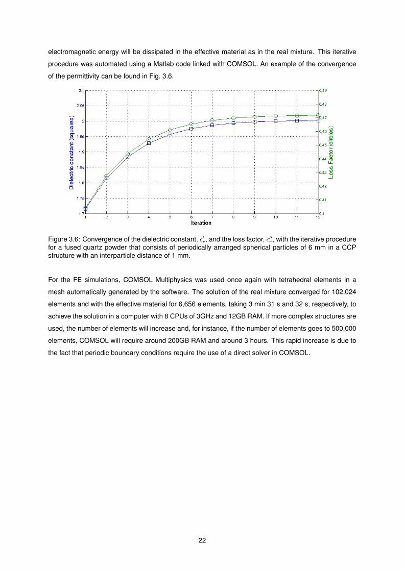
electromagnetic energy will be dissipated in the effective material as in the real mixture. This iterative

procedure was automated using a Matlab code linked with COMSOL. An example of the convergence

of the permittivity can be found in Fig. 3.6.

Figure 3.6: Convergence of the dielectric constant, ε′r, and the loss factor, ε′′r , with the iterative procedurefor a fused quartz powder that consists of periodically arranged spherical particles of 6 mm in a CCPstructure with an interparticle distance of 1 mm.

For the FE simulations, COMSOL Multiphysics was used once again with tetrahedral elements in a

mesh automatically generated by the software. The solution of the real mixture converged for 102,024

elements and with the effective material for 6,656 elements, taking 3 min 31 s and 32 s, respectively, to

achieve the solution in a computer with 8 CPUs of 3GHz and 12GB RAM. If more complex structures are

used, the number of elements will increase and, for instance, if the number of elements goes to 500,000

elements, COMSOL will require around 200GB RAM and around 3 hours. This rapid increase is due to

the fact that periodic boundary conditions require the use of a direct solver in COMSOL.

22

Chapter 4

Results

The results obtained with the developed method and model are presented in this chapter. First, the

convergence procedures used for the numerical simulations and for the iterative process are presented

in Sec. 4.1. In Sec. 4.2, the tested materials are described, the resulting properties showed, an inter-

pretation of the results is given and the consistency of the created method is put to the test. To show

the electromagnetic and thermal behaviour of the extracted properties, a comparison between different

models is given in Sec. 4.3.

4.1 Convergence of the simulations and of the iterative process

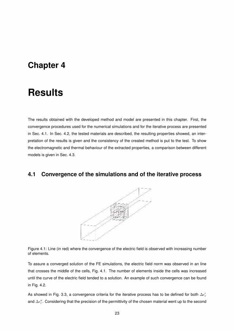
Figure 4.1: Line (in red) where the convergence of the electric field is observed with increasing numberof elements.

To assure a converged solution of the FE simulations, the electric field norm was observed in an line

that crosses the middle of the cells, Fig. 4.1. The number of elements inside the cells was increased

until the curve of the electric field tended to a solution. An example of such convergence can be found

in Fig. 4.2.

As showed in Fig. 3.3, a convergence criteria for the iterative process has to be defined for both ∆ε′r

and ∆ε′′r . Considering that the precision of the permittivity of the chosen material went up to the second

23

Figure 4.2: Convergence of the electric field norm curve inside the line showed in Fig. 4.1.

decimal value, the increments have to be lower then 0.001 for the permittivity value to be considered

converged. This was the chosen criteria. The number of iterations for both ε′r and ε′′r to converge for the

case study detailed in the next section was 12 iterations, as can be seen in Fig. 3.6.

4.2 Case studies and tests

The simulations were conducted for a fused quartz powder that consists of periodically arranged spher-

ical particles of diameter φ = 6mm in a CCP structure with an interparticle distance of 1 mm and for

φ = 2mm with an interparticle distance of 0.33 mm. This material was chosen for being a dielectric

(σ ≈ 0), for not responding to the magnetic field (µ = µ0) and for having a complex permittivity at room

temperature, εr(25C) = 3.78 − j2.27 [49], constituting a simple case study. The host material in the

mixture is air. The material’s microscopic properties and the resulting effective properties which have

been calculated according to Chapter 3 for the φ = 6mm material can be found in Tab. 4.1 .

Properties: Quartz (25C) Air (25C) Effective materialε′r 3.78 1 2.00ε′′r 2.27 0 0.47µr 1 1 1σ[S/m] 1× 10−12 3× 10−15 3× 10−15

ρ[kg/m3] 2600.0 1.1839 1176.89cp[J/(kg ·K] 820.00 1005.0 820.11κ[W/(m ·K)] 3.00 0.024 0.089

Table 4.1: Properties of quartz, air and of the effective material with periodically arranged sphericalparticles of diameter φ = 6mm in a CCP structure with an interparticle distance of 1 mm

The effective complex permittivity obtained for φ = 6mm was εr = 2.00− j0.47. Taking into account that

the simulated mixture is a pure dielectric, which means that the waves penetrate the entire material, and

that the host of the mixture has a εr = 1, the value obtained is an expected value. The same can be said

24

for the results from the simulation of the same structure with spheres of φ = 2mm and an interparticle

distance of 0.33 mm where the obtained effective permittivity was εr = 1.99− j0.46. The results are so

close to each other because the volume fraction of inclusions was kept constant. All the above results

were obtained for three cells repeated in the z-direction as showed in Fig. 3.4 and Fig. 3.5.

Figure 4.3: Power flow (green line), electric (blue line) and magnetic field norm (red line) in a line withz-direction that passes through the middle of the three cells with the heterogeneous material.

For interpretation purposes, Fig. 4.3 shows the power flow, electric and magnetic field norm in a line

that passes through the middle of the three cells with the heterogeneous material. It can be seen that

the electric field oscillates sharply inside the cells (between z = 47mm and z = 77mm), which is due

to the induction mechanisms and existing reflections in the interfaces between the two material, quartz

and air. Between the emitting port (z = 0mm) and the beginning of the cells, smoother oscillations exist

due to the resonance frequency obtained from the interacting incoming waves with the waves reflected

by the cells. After the cells, both electric and magnetic fields take a constant value. This is due to the

non-reflective boundary in the end of the domain, so no reflections exist after the wave passes through

the cells and the constant fields represent a plane wave travelling through space. The emitted power

flow is constant before and after the cells, the difference between those values represent the total power

dissipated to heat Qem in the material. The oscillations in the power flow are due to the oscillations in

the electric field as it is known from Eq. 2.24 that it has a quadratic dependence of the electric field. In

the magnetic field, there are no oscillations inside the material for there is no absorption and dissipation

of the magnetic field. Nevertheless, it can be observed slight discontinuities in the material interfaces.

The improvement of the effective permittivity throughout the iterative process is clearly showed in Fig. 4.4,

where the electric and magnetic fields of the effective materials tend to the shape of the fields of the

mixture. The existing oscillations in the mixture fields relative to effective fields are due to the interfaces

between two media inside the mixture as it was commented previously.

To test the quality of the effective permittivity, a series of runs were made to see if a good homogenization

was performed with the selected sample. Considering that, in fact, the chosen periodic cubic sample

25

(a)

(b)

Figure 4.4: Effect of the evolution of permittivity on the electric, Fig. 4.4(a), and magnetic fields,Fig. 4.4(b), of the effective material in a line that passes through the middle of the cells with the z-direction. The arrows represent the tendency of the evolution throughout the iterative process. Thedashed dark blue lines represent the fields of the mixture.

is representative of a material, the obtained effective permittivity should not vary when the size of the

sample is increased. Indeed, when the number of cells in the direction of the propagation of the wave

was increased, a maximum variation of 1.5% in ε′r and 6.5% in ε′′r was found. The results of this test are

presented in Tab. 4.2 in the all cells columns for the φ = 6mm and φ = 2mm materials. If the cells are

collocated in different positions relative to the wave, the exact same values are obtained. To check if the

periodic boundary conditions were describing well the material, an increase of the number of cells in the

26

φ = 6mm φ = 2mmall cells 1 cell all cells 1 cell

N of cells ε′r ε′′r ε′r ε′′r ε′r ε′′r ε′r ε′′r1 1.97 0.49 1.97 0.49 1.99 0.49 1.99 0.493 2.00 0.47 1.72 0.39 1.99 0.46 1.97 0.455 1.97 0.46 1.99 0.45 1.98 0.46 1.95 0.447 1.99 0.46 1.98 0.45 1.99 0.46 1.87 0.429 1.97 0.45 1.64 0.37 2.00 0.46 1.60 0.36

Table 4.2: Results for test of checking the effect of increasing the number of cells in the extractedpermittivity for φ = 6mm and φ = 2mm materials. all cells stands for We and Qem measured in all theexisting cells and 1 cell stands for We and Qem measured only in the middle cell.

x- and y- directions was tested, resulting in the same value of the effective permittivity. In all the above

mentioned results, We andQem were measured in all the existing cells in the domain. If we only measure

in one cell and study the effect of increasing number of neighbour cells, effects of relative positioning

of the cell to the wave inside the cells (the wavelength inside a material is different from outside the

material) will make the permittivity values oscillate up to 26%. For this reason, this last approach is not

recommended. The results of this test are presented in Tab. 4.2 in the 1 cell columns.

4.3 Comparison between different models

Microwave heating of the characterized samples were simulated in the single mode (TE10) cavity in

order to compare the heating profiles of the mixture with the effective material. The cavity boundaries

consist of one port in the -z limit and perfect electric conductors in the rest of the walls. The cubic sample

was positioned in the peak of the electric field as can be seen in Fig. 4.5.

Figure 4.5: Electric field norm distribution inside the cavity with a sample with effective properties. Thefigure uses a coloured plot in a plane that intercepts the sample to show the electric field intensity. Thecubic sample is located inside the cavity in the peak of the electric field norm, red region.

Despite the fact that the boundary conditions around the sample inside the cavity do not represent the

infinite extent of the material, which makes this model unsuitable for an homogenization procedure,

the developed method can still be performed with this model and a permittivity can be obtained. The

27

advantage of using this model instead of the plane wave model is that it is closer to the case of a

real sample being heated inside a microwave oven and using the created method can guarantee that

the mixture will have the same We and Qem as the effective mixture. To compare the electromagnetic

and heating behaviour of the mixture with the sample with the effective properties, simulations were

performed using the cavity of Fig. 4.5 and a sample of 1 cm3 with:

• The mixture with φ = 2mm spheres;

• The bulk material with effective properties obtained with the plane wave model;

• The bulk material with effective properties obtained with the cavity model.

In Tab. 4.3, it can be verified that the cavity model gives closer We and Qem to the mixture; however, the

rest of the parameters have very proximate values.

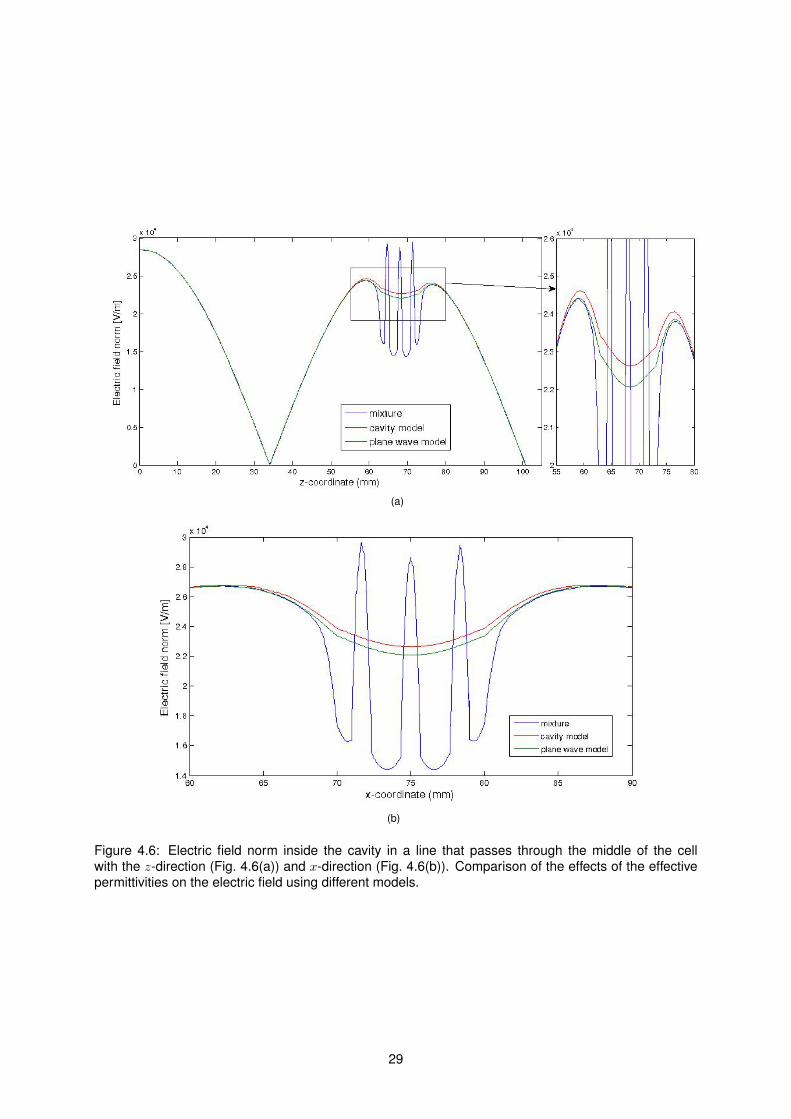
If one looks at the electric fields inside the cavity and the samples an interesting result can be found.

The electric field norm curve near and inside the sample of the plane wave model follows the mixture

curve much better than the cavity model. Such result can be observed in Fig. 4.6. This shows the quality

of the homogenization performed with the plane wave model.

Model: Mixture Plane wave Cavityε′reff

- 1.99 1.88ε′′reff

- 0.46 0.45We[J/m

3] 2.0827e-3 2.1065e-3 2.0818e-3Qe[W/m3] 1.5257e7 1.4859e7 1.5250e7HR [C/s] 15.2 15.4 15.8S11 [dB] 0.0668 0.0650 0.0667

Table 4.3: Results of the electromagnetic and heating response of the different models. HR stands forHeating Rate.

28

(a)

(b)

Figure 4.6: Electric field norm inside the cavity in a line that passes through the middle of the cellwith the z-direction (Fig. 4.6(a)) and x-direction (Fig. 4.6(b)). Comparison of the effects of the effectivepermittivities on the electric field using different models.

29

30

Chapter 5

Conclusions

This thesis presents a new energy based method for characterization of the effective dielectric properties

of a heterogeneous material. With the material’s properties and their micro-structure, all the effective

macro-properties needed for the modelling of microwave heating can be obtained. The method was

demonstrated for a powder consisting of spherical inclusions in a CCP structure.

This method uses an iterative procedure to improve the estimates of the effective complex permittivity

based on the stored electric energy and dissipated electromagnetic energy. With a Matlab code, the

FE simulations performed in COMSOL were carried out automatically in order to make the iterative

process faster and less wearing. The FE simulations needed to extract the permittivity only include the

electromagnetic waves physics. The simulations done to compare the different model geometries also

used the heat transfer physics. Simulations with multiphysics are more computationally expensive.

An interpretation of the resulting fields from the performed simulations was made considering the existing

effects in the passage of a plane wave throughout the micro-structure of a dielectric material.

5.1 Achievements

On the modelling side, a periodic cubic sample being irradiated by microwaves surrounded of periodic

boundary conditions allows the extraction of a consistent effective permittivity. The improvement of the

effective permittivity throughout the iterative procedure results in electromagnetic fields closer to the

ones of the heterogeneous material. The permittivity obtained using this model enables the effective

material to get a smooth electric field very close to the one of the real mixture, while respecting the

thermal response and the ability of the material to store and dissipate electric energy.

31

5.2 Future Work

Although the present results seem promising, it is clear that new tests in inhomogeneous materials

should be carried out with the present methodology. Comparison with existing theoretical models and

available experimental results will allow a greater understanding of the method. Adapting the method

to also obtain the effective permeability of magnetic sensitive materials in an analogous way to the

permittivity, will allow the increase of the range of applications. Special interest lays in the use of this

method to study the introduction of susceptors in materials for microwave heating applications.

32

Bibliography

[1] D. Agrawal, J. Cheng, H. Peng, L. Hurt, and K. Cherian. Microwave energy applied to processing

of high-temperature materials. American Ceramic Society Bulletin, 87(3):39, 2008.

[2] A.C. Metaxas. Foundations of electroheat: a unified approach. Wiley, 1996. ISBN 9780471956440.

[3] D.M. Pozar. Microwave Engineering, 3Rd Ed. Wiley India Pvt. Limited, 2009. ISBN 9788126510498.

[4] S. Chandrasekaran, T. Basak, and S. Ramanathan. Experimental and theoretical investigation on

microwave melting of metals. Journal of Materials Processing Technology, 211(3):482 – 487, 2011.

ISSN 0924-0136.

[5] D.E. Clark, D.C. Folz, C.E. Folgar, and M.M. Mahmoud. Microwave Solutions for Ceramic Engi-

neers. Wiley, 2005. ISBN 9781574982244.

[6] Y.V. Bykov, K.I. Rybakov, and V.E. Semenov. High-temperature microwave processing of materials.

Journal of Physics D: Applied Physics, 34(13):R55, 2001.

[7] C. Brosseau, P. Queffelec, and P. Talbot. Microwave characterization of filled polymers. Journal of

Applied Physics, 89(8):4532–4540, 2001.

[8] S. Huclova, D. Erni, and J. Frohlich. Modelling effective dielectric properties of materials containing

diverse types of biological cells. Journal of Physics D: Applied Physics, 43(36):365405, 2010.

[9] K. Karkkainen, A. Sihvola, and K. Nikoskinen. Analysis of a three-dimensional dielectric mixture

with finite difference method. Geoscience and Remote Sensing, IEEE Transactions on, 39(5):

1013–1018, May 2001. ISSN 0196-2892. doi: 10.1109/36.921419.

[10] A. Alu. First-principles homogenization theory for periodic metamaterials. Physical Review B, 84

(7):075153, 2011.

[11] D. Wu, J. Chen, and C. Liu. Numerical evaluation of effective dielectric properties of three-

dimensional composite materials with arbitrary inclusions using a finite-difference time-domain

method. Journal of Applied Physics, 102(2):024107–024107–8, Jul 2007. ISSN 0021-8979. doi:

10.1063/1.2756089.

[12] B. Sareni, L. Krahenbuhl, A. Beroual, and C. Brosseau. Complex effective permittivity of a lossy

composite material. Journal of applied physics, 80(8):4560–4565, 1996.

33

[13] B. Sareni, L. Krahenbuhl, A. Beroual, and C. Brosseau. Ab Initio simulation approach for calculating

the effective dielectric constant of composite materials. Journal of electrostatics, 40:489–494, 1997.

[14] C. Brosseau and A. Beroual. Computational electromagnetics and the rational design of new di-

electric heterostructures. Progress in Materials Science, 48(5):373–456, 2003.

[15] A. Boudida, A. Beroual, and C. Brosseau. Permittivity of lossy composite materials. Journal of

applied physics, 83(1):425–431, 1998.

[16] I. Krakovsky and V. Myroshnychenko. Modeling dielectric properties of composites by finite-element

method. Journal of applied physics, 92(11):6743–6748, 2002.

[17] C. Brosseau. A finite-element simulation study of the complex effective permittivity of two-phase

random composite materials. In COMSOL Multiphysics Users Conference 2005, 2005.

[18] V. Myroshnychenko and C. Brosseau. Finite-element method for calculation of the effective permit-

tivity of random inhomogeneous media. Physical Review E, 71(1):016701, 2005.

[19] V. Myroshnychenko and C. Brosseau. Finite-element modeling method for the prediction of the

complex effective permittivity of two-phase random statistically isotropic heterostructures. Journal

of applied physics, 97(4):044101, 2005.

[20] Y. Cheng, X. Chen, K. Wu, S. Wu, Y. Chen, and Y. Meng. Modeling and simulation for effective

permittivity of two-phase disordered composites. Journal of Applied Physics, 103(3):034111, 2008.

[21] V. Myroshnychenko and C. Brosseau. Effective complex permittivity and continuum percolation

analysis of two-phase composite media. Dielectrics and Electrical Insulation, IEEE Transactions

on, 16(4):1209–1222, 2009.

[22] V. Myroshnychenko and C. Brosseau. Analysis of the effective permittivity in percolative composites

using finite element calculations. Physica B: Condensed Matter, 405(14):3046–3049, 2010.

[23] N. Jebbor and S. Bri. Effective permittivity of periodic composite materials: Numerical modeling by

the finite element method. Journal of Electrostatics, 70(4):393–399, 2012.

[24] L. Xu, C. Liu, Z. Cao, and X. Li. Particle size influence on effective permittivity of particle–gas

mixture with particle clusters. Particuology, 11(2):216–224, 2013.

[25] J.P. Calame, A. Birman, Y. Carmel, D. Gershon, B. Levush, A.A. Sorokin, V.E. Semenov, D. Dadon,

L.P. Martin, and M. Rosen. A dielectric mixing law for porous ceramics based on fractal boundaries.

Journal of applied physics, 80(7):3992–4000, 1996.

[26] D. Gershon, J.P. Calame, and A. Birnboim. Complex permittivity measurements and mixing laws of

porous alumina. Journal of Applied Physics, 89(12):8117–8120, 2001.

[27] J. Peon-Fernandez, J. Martın-Herrero, N. Banerji, and T.P. Iglesias. Numerical study of effective

permittivity in composite systems. Applied surface science, 226(1):78–82, 2004.

34

[28] Y.V. Serdyuk, A.D. Podoltsev, and S.M. Gubanski. Numerical simulations of dielectric properties of

composite material with periodic structure. Journal of electrostatics, 63(11):1073–1091, 2005.

[29] L. Jylha, J. Honkamo, H. Jantunen, and A. Sihvola. Microstructure-based numerical modeling

method for effective permittivity of ceramic/polymer composites. Journal of applied physics, 97(10):

104104, 2005.

[30] L. Jylha and A.H. Sihvola. Numerical modeling of disordered mixture using pseudorandom simula-

tions. Geoscience and Remote Sensing, IEEE Transactions on, 43(1):59–64, 2005.

[31] A. Mejdoubi and C. Brosseau. Controllable effective complex permittivity of functionally graded

composite materials: A numerical investigation. Journal of Applied Physics, 102(9):094105, 2007.

[32] C. Fourn, S. Lasquellec, and C. Brosseau. Finite-element modeling method for the study of di-

electric relaxation at high frequencies of heterostructures made of multilayered particle. Journal of

Applied Physics, 102(12):124107, 2007.

[33] M.G. Silveirinha. Metamaterial homogenization approach with application to the characterization of

microstructured composites with negative parameters. Physical Review B, 75(11):115104, 2007.

[34] J.T. Costa, M.G. Silveirinha, and S.I. Maslovski. Finite-difference frequency-domain method for the

extraction of effective parameters of metamaterials. Physical Review B, 80(23):235124, 2009.

[35] K.K. Karkkainen, A.H. Sihvola, and K.I. Nikoskinen. Effective permittivity of mixtures: Numerical

validation by the fdtd method. Geoscience and Remote Sensing, IEEE Transactions on, 38(3):

1303–1308, 2000.

[36] T. Weiland, R. Schuhmann, R.B. Greegor, C.G. Parazzoli, A.M. Vetter, D.R. Smith, D.C. Vier, and

S. Schultz. Ab initio numerical simulation of left-handed metamaterials: Comparison of calculations

and experiments. Journal of Applied Physics, 90(10):5419–5424, 2001.

[37] T. Galek, K. Porath, E. Burkel, and U. van Rienen. Extraction of effective permittivity and perme-

ability of metallic powders in the microwave range. Modelling and Simulation in Materials Science

and Engineering, 18(2):025015, 2010.

[38] L. Liu, S.M. Matitsine, Y.B. Gan, and K.N. Rozanov. Effective permittivity of planar composites with

randomly or periodically distributed conducting fibers. Journal of applied physics, 98(6):063512,

2005.

[39] C.C. Njoku, W.G. Whittow, and J.C. Vardaxoglou. Effective permittivity of heterogeneous substrates

with cubes in a 3-d lattice. Antennas and Wireless Propagation Letters, IEEE, 10:1480–1483, 2011.

[40] M. J. Akhtar T. Gupta and A. Biswas. A unit cell approach to model and characterize the metal

powders and metal-dielectric composites at microwave frequencies. Progress In Electromagnetics

Research B, 49(2):363–387, 2013.

[41] E. Tuncer and I. Sauers. Effective dielectric properties of binary dielectric mixtures on checker-

35

boards. In Electrical Insulation and Dielectric Phenomena (CEIDP), 2012 Annual Report Confer-

ence on, pages 633–636. IEEE, 2012.

[42] A.H. Sihvola and Institution of Electrical Engineers. Electromagnetic Mixing Formulas and Applica-

tions. IEE Publication Series. Institution of Electrical Engineers, 1999. ISBN 9780852967720.

[43] R. G. Martın. Electromagnetic field theory for physicists and engineers: Fundamentals and Appli-

cations. 2006.

[44] L. Chen. Microwave electronics: measurement and materials characterization. John Wiley, 2004.

ISBN 9780470844922.

[45] S. Ramo, J. R. Whinnery, and T. Van Duzer. Fields and Waves in Communication Electronics. Wiley,

1994. ISBN 9780471585510.

[46] M. Mehdizadeh. Microwave/RF Applicators and Probes for Material Heating, Sensing, and Plasma

Generation: A Design Guide. Elsevier Science, 2009. ISBN 9780815519867.

[47] B. Thide. Electromagnetic Field Theory. Dover Publications, Incorporated, 2011. ISBN

9780486477732.

[48] X. Zhao, L. Yan, and K. Huang. Review of numerical simulation of microwave heating process.

Advances in Induction and Microwave Heating of Mineral and Organic Materials, pages 27–48,

2011.

[49] A.R. Von Hippel. Dielectric materials and applications. Artech House microwave library. Artech

House, 1954. ISBN 9780890068052.

36

Appendix A

Vector calculus

Some definitions and vector identities are listed in the section below.

A.1 Vector identities

∇× (∇φ) = 0 (A.1)

∇ · (∇× ~U) = 0 (A.2)

∇ · ( ~A× ~B) = ~B · ∇ × ~A− ~A · ∇ × ~B (A.3)

37

38