ALGORITHM REFINEMENT FOR FLUCTUATINGHYDRODYNAMICS∗
SARAH A. WILLIAMS† , JOHN B. BELL‡ , AND ALEJANDRO L. GARCIA§
Abstract. This paper introduces an adaptive mesh and algorithm refinement method for fluc-tuating hydrodynamics. This particle-continuum hybrid simulates the dynamics of a compressiblefluid with thermal fluctuations. The particle algorithm is direct simulation Monte Carlo (DSMC),a molecular-level scheme based on the Boltzmann equation. The continuum algorithm is based onthe Landau–Lifshitz Navier–Stokes (LLNS) equations, which incorporate thermal fluctuations intomacroscopic hydrodynamics by using stochastic fluxes. It uses a recently developed solver for theLLNS equations based on third-order Runge–Kutta. We present numerical tests of systems in andout of equilibrium, including time-dependent systems, and demonstrate dynamic adaptive refinementby the computation of a moving shock wave. Mean system behavior and second moment statisticsof our simulations match theoretical values and benchmarks well. We find that particular attentionshould be paid to the spectrum of the flux at the interface between the particle and continuummethods, specifically for the nonhydrodynamic (kinetic) time scales.
Key words. stochastic Navier–Stokes equations, multiscale hybrid algorithm, computationalfluid dynamics, direct simulation Monte Carlo, adaptive mesh refinement
1. Introduction. Adaptive mesh refinement (AMR) is often employed in com-putational fluid dynamics (CFD) simulations to improve efficiency and/or accuracy:a fine mesh is applied in regions where high resolution is required for accuracy, anda coarser mesh is applied elsewhere to moderate computational cost. For dynamicproblems, the area that is a candidate for mesh refinement may change over time,so methods have been developed to adaptively identify the refinement target area ateach time step (e.g., [9, 8, 5]).
However, at the smallest scales, on the order of a molecular mean free path,continuum assumptions may not hold, so CFD approaches do not accurately modelthe relevant physics. In such a regime, adaptive mesh and algorithm refinement(AMAR) improves on AMR by introducing a more physically accurate particle methodto replace the continuum solver on the finest mesh. An improved simulation doesnot result from continued refinement of the mesh but rather from “refinement” ofthe algorithm, i.e., switching from the continuum model to a particle simulation.Introduced in [26], AMAR has proved to be a useful paradigm for multiscale fluidmodeling. In this paper, we describe AMAR for fluctuating hydrodynamics.
Random thermal fluctuations occur in fluids at microscopic scales (considerBrownian motion), and these microscopic fluctuations can lead to macroscopic sys-
∗Received by the editors July 3, 2007; accepted for publication (in revised form) October 24,2007; published electronically February 1, 2008. This work was supported in part by the AppliedMathematics Program of the DOE Office of Mathematics, Information, and Computational Sciencesunder the U.S. Department of Energy under contract DE-AC02-05CH11231.
http://www.siam.org/journals/mms/6-4/69618.html†Department of Mathematics, University of North Carolina at Chapel Hill, Phillips Hall CB 3250,
Chapel Hill, NC 27599 ([email protected]).‡Center for Computational Sciences and Engineering, Lawrence Berkeley National Laboratory, 1
Cyclotron Road, MS 50A-1148, Berkeley, CA 94720 ([email protected]).§Department of Physics, San Jose State University, 1 Washington Square, San Jose, CA 95192
ALGORITHM REFINEMENT FOR FLUCTUATING HYDRODYNAMICS 1257
tem effects. The correct treatment of fluctuations is especially important for sto-chastic nonlinear systems, such as those undergoing phase transitions, nucleation,noise-driven instabilities, and combustive ignition. In these and related applications,nonlinearities can exponentially amplify the influence of the fluctuations. As an ex-ample, consider the classical Rayleigh–Taylor problem and the related Richtmyer–Meshkov instability that are prototypical problems for the study of turbulent mixing.A heavy fluid sits above a light fluid, and spontaneous microscopic fluctuation at theinterface between the fluids leads to turbulent mixing throughout the domain. Kadauand coworkers have recently studied the development of this turbulence at the atomicscale [35, 36]. That group’s atomistic simulations indicate that thermal fluctuationsare an important driver of the behavior of complex flows, certainly at the smallestscales and perhaps at all scales. For example, in stochastic atomistic simulations ofRayleigh–Taylor, and in laboratory experiments, spikes of the heavy fluid that projectinto the light fluid can break off to form isolated droplets; this phenomenon cannot bereproduced accurately by deterministic continuum models. However, the physical andtemporal domain on which this type of atomistic simulation is computationally feasibleis extremely limited (less than a billion atoms per nanosecond) given current algo-rithms and near-term computational power. Other examples in which spontaneousfluctuations play a key role include the breakup of droplets in nanojets [47, 20, 37],Brownian molecular motors [33, 50, 18, 45], exothermic reactions [49, 41], such as incombustion and explosive detonation, and reaction fronts [46]. The goal of AMARfor fluctuating hydrodynamics is to effectively enhance the computing power availablefor investigations of these types of phenomena.
Hadjiconstantinou reviewed theoretical and numerical approaches to challengesarising from the breakdown of the Navier–Stokes description at small scale and (withWijesinghe) described a variety of particle-continuum methods for multiscale hydro-dynamics [55, 32]. The work presented here is the latest effort in a line of work that hasfocused on building AMAR hybrids for flows of increasing sophistication. A hybridcoupling Navier–Stokes and direct simulation Monte Carlo (DSMC) was developedin [26], with several of the technical issues necessary for implementation extended in[56]. Stochastic hybrid methods were developed in [2] (mass diffusion), [3] (the “trainmodel” for momentum diffusion), and [6] (Burgers’s equation). Other recent workon coupling particle and continuum methods includes [53] (DSMC and Navier–Stokesfor aerospace applications), [30, 17] (molecular dynamics and isothermal fluctuatinghydrodynamics for polymer simulations), and [39] (an adaptive refinement approachbased on a direct numerical solution of the Boltzmann transport equation and kineticcontinuum schemes).
The AMAR approach is characterized by several design principles. In contrastto other algorithm refinement approaches (see, e.g., [16]), in AMAR (as in AMR) thesolution of the macroscopic model is maintained over the entire domain. A refinementcriterion is used to estimate where the improved representation of the particle methodis required. That region, which can change dynamically, is then “covered” with aparticle patch. In this hierarchical representation, upon synchronization the particlesolution replaces the continuum solution in the regions covered by the molecularpatches.
Given their complexity, the implementations of hybrid codes benefit greatly frommodularization (e.g., see [53]). Another fundamental tenet of the AMAR approach toparticle-continuum hybridization is that the coupling of the two algorithms is com-pletely encapsulated in several “hand-shaking” routines. Taken as a unit, the particlemethod plus these modular routines perform exactly the same function as any fine
grid in a single-algorithm AMR method. The encapsulated coupling routines performthe following functions: continuum data is used to generate particles that flow into theparticle region; flux across the boundaries of the particle region is recorded and usedto correct neighboring continuum values; cell-averaged data from the particle gridreplaces data on the underlying continuum grid; continuum data is used to generateparticles to initialize new particle regions identified by the refinement criterion.
Implementation details are given in the next two sections of the paper. Our con-tinuum approach for fluctuating hydrodynamics is an explicit finite volume method forsolving the Landau–Lifshitz Navier–Stokes (LLNS) equations for compressible fluidflow (see section 2.1) and, as noted above, the particle method is DSMC (see sec-tion 2.2). Hybrid coupling details are discussed in section 3. Numerical resultsfor problems with a static refinement region are presented in section 4 for a va-riety of steady-state and time-dependent problems with the flow restricted to onespatial dimension. (Forthcoming work will illustrate this construction extended totwo- and three-dimensional systems.) Details of adaptive refinement are discussedin section 4.5, including numerical results for an adaptive refinement shock-trackingproblem. We conclude, in section 5, with a discussion of future work.
2. Components of the hybrid.
2.1. Continuum approach. The continuum model and solver discussed in thissection was introduced in [7], and the reader is referred to that paper for furtherdetails of the method and measurements of its performance.
To incorporate thermal fluctuations into macroscopic hydrodynamics, Landauand Lifshitz introduced an extended form of the Navier–Stokes equations by addingstochastic flux terms [40]. The LLNS equations have been derived by a variety ofapproaches (see [40, 12, 21, 38, 13]), and while they were originally developed forequilibrium fluctuations, validity of the LLNS equations for nonequilibrium systemshas been derived [48] and verified in molecular simulations [29, 42, 44].
The LLNS equations may be written as
(1) ∂U/∂t + ∇ · F = ∇ · D + ∇ · S,where
U =
⎛⎝ ρ
JE
⎞⎠
is the vector of conserved quantities (density of mass, momentum, and energy).The hyperbolic flux is given by
F =
⎛⎝ ρv
ρvv + P I(E + P )v
⎞⎠ ,
and the diffusive flux is given by
D =
⎛⎝ 0
ττ · v + κ∇T
⎞⎠ ,
where v is the fluid velocity, P is the pressure, T is the temperature, and τ =η(∇v + ∇vT − 2
3I∇ · v) is the stress tensor. Here η and κ are coefficients of vis-cosity and thermal conductivity, respectively, where we have assumed that the bulkviscosity is zero.
ALGORITHM REFINEMENT FOR FLUCTUATING HYDRODYNAMICS 1259
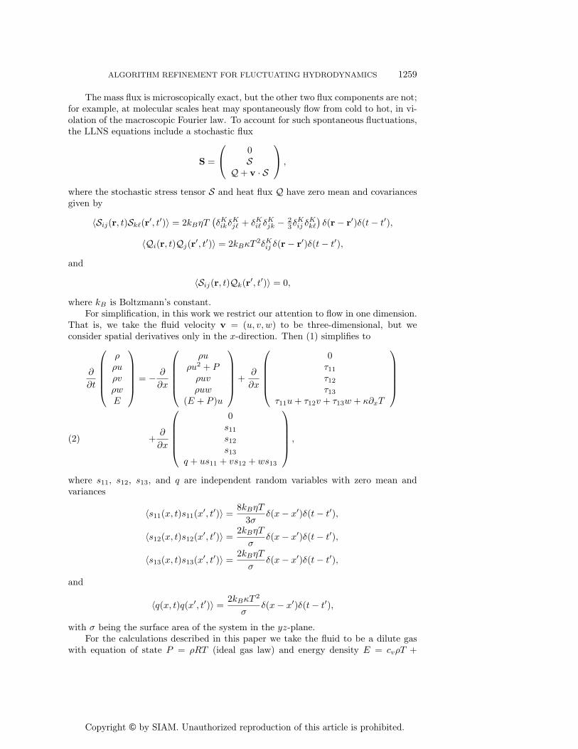
The mass flux is microscopically exact, but the other two flux components are not;for example, at molecular scales heat may spontaneously flow from cold to hot, in vi-olation of the macroscopic Fourier law. To account for such spontaneous fluctuations,the LLNS equations include a stochastic flux
S =
⎛⎝ 0
SQ + v · S
⎞⎠ ,
where the stochastic stress tensor S and heat flux Q have zero mean and covariancesgiven by
〈Sij(r, t)Sk�(r′, t′)〉 = 2kBηT
(δKikδ
Kj� + δKi� δ
Kjk − 2
3δKij δ
Kk�
)δ(r − r′)δ(t− t′),
〈Qi(r, t)Qj(r′, t′)〉 = 2kBκT
2δKij δ(r − r′)δ(t− t′),
and
〈Sij(r, t)Qk(r′, t′)〉 = 0,
where kB is Boltzmann’s constant.For simplification, in this work we restrict our attention to flow in one dimension.
That is, we take the fluid velocity v = (u, v, w) to be three-dimensional, but weconsider spatial derivatives only in the x-direction. Then (1) simplifies to
∂
∂t
⎛⎜⎜⎜⎜⎝
ρρuρvρwE
⎞⎟⎟⎟⎟⎠ = − ∂
∂x
⎛⎜⎜⎜⎜⎝
ρuρu2 + Pρuvρuw
(E + P )u
⎞⎟⎟⎟⎟⎠ +
∂
∂x
⎛⎜⎜⎜⎜⎝
0τ11τ12τ13
τ11u + τ12v + τ13w + κ∂xT
⎞⎟⎟⎟⎟⎠
+∂
∂x
⎛⎜⎜⎜⎜⎝
0s11
s12
s13
q + us11 + vs12 + ws13
⎞⎟⎟⎟⎟⎠ ,(2)
where s11, s12, s13, and q are independent random variables with zero mean andvariances
〈s11(x, t)s11(x′, t′)〉 =
8kBηT
3σδ(x− x′)δ(t− t′),
〈s12(x, t)s12(x′, t′)〉 =
2kBηT
σδ(x− x′)δ(t− t′),
〈s13(x, t)s13(x′, t′)〉 =
2kBηT
σδ(x− x′)δ(t− t′),
and
〈q(x, t)q(x′, t′)〉 =2kBκT
2
σδ(x− x′)δ(t− t′),
with σ being the surface area of the system in the yz-plane.For the calculations described in this paper we take the fluid to be a dilute gas
with equation of state P = ρRT (ideal gas law) and energy density E = cvρT +
2 +v2 +w2). The transport coefficients are only functions of temperature; specif-
ically we take them as η = η0
√T and κ = κ0
√T , where the constants η0 and κ0 are
chosen to match the viscosity and thermal conductivity of a hard sphere gas. We alsohave gas constant R = kB/m and cv = R
γ−1 , where m is the mass of a particle and
the ratio of specific heats is taken to be γ = 53 , that is, a monatomic gas. Note that
generalizations of fluid parameters are straightforward, and the choice of a monatomichard sphere gas is for convenience in matching parameters in the PDE with those ofDSMC simulations (see section 2.2).
The principal difficulty in solving (2) arises because there is no stochastic forcingterm in the mass conservation equation. Accurately capturing density fluctuationsrequires that the fluctuations be preserved in computing the mass flux. Another keyobservation is that the representation of fluctuations in CFD schemes is also sensi-tive to the time step, with extremely small time steps leading to improved results.This suggests that temporal accuracy also plays a significant role in capturing fluctu-ations. Based on these observations, a discretization aimed specifically at capturingfluctuations in the LLNS equations has been developed [7]. The method is based ona third-order, total variation diminishing (TVD) Runge–Kutta temporal integrator(RK3) [31, 51] combined with a centered discretization of hyperbolic and diffusivefluxes.
The RK3 discretization can be written in the following three-stage form:
Un+1/3j = Un
j − Δt
Δx(Fn
j+1/2 −Fnj−1/2),
Un+2/3j =
3
4Un
j +1
4U
n+1/3j − 1
4
(Δt
Δx
)(Fn+1/3
j+1/2 −Fn+1/3j−1/2 ),
Un+1j =
1
3Un
j +2
3U
n+2/3j − 2
3
(Δt
Δx
)(Fn+2/3
j+1/2 −Fn+2/3j−1/2 ),
where Fm = F(Um) − D(Um) − S̃(Um) and S̃ =√
2S. The diffusive terms Dare discretized with standard second-order finite difference approximations. In theapproximation to the stochastic stress tensor, S̃j+1/2, the terms are computed as
smn =
√kB
ΔtVc
(1 + 1
3δKmn
)(ηj+1Tj+1 + ηjTj) �j+1/2,
where Vc = σΔx is the volume of a cell and the �’s are independent Gaussian dis-tributed random values with zero mean and unit variance. Similarly, the discretizedstochastic heat flux is evaluated as
ALGORITHM REFINEMENT FOR FLUCTUATING HYDRODYNAMICS 1261
The variance in the stochastic flux at j + 1/2 is given by
〈(SΣj+1/2)
2〉 =
⟨(1
6(S̃n
j+1/2) +1
6(S̃
n+1/3j+1/2 ) +
2
3(S̃
n+2/3j+1/2 )
)2⟩
=
(1
6
)2
〈(S̃nj+1/2)
2〉 +
(1
6
)2
〈(S̃n+1/3j+1/2 )2〉 +
(2
3
)2
〈(S̃n+2/3j+1/2 )2〉.
Neglecting the multiplicity in the noise, we obtain the desired result that 〈(SΣ)2〉 =12 〈(S̃)2〉 = 〈(S)2〉; that is, taking S̃ =
√2S corrects for the reduction of the stochastic
flux variance due to the three-stage averaging of the fluxes. However, this treatmentdoes not directly affect the fluctuations in density, since the component of S in thecontinuity equation is zero. The density fluctuations are controlled by the spatialdiscretization. To compensate for the suppression of density fluctuations due to thetemporal averaging, we interpolate the momentum J = ρu (and the other conservedquantities) from cell-centered values:
(3) Jj+1/2 = α1(Jj + Jj+1) − α2(Jj−1 + Jj+2),
where
α1 = (√
7 + 1)/4 and α2 = (√
7 − 1)/4.
Then in the case in which J is statistically stationary and constant in space we haveexactly Jj+1/2 = J and 〈δJ2
j+1/2〉 = 2〈δJ2〉, as desired; the interpolation is consis-tent and compensates for the variance-reducing effect of the multistage Runge–Kuttaalgorithm.
The stochastic flux in our numerical schemes for the LLNS equations is a multi-plicative noise since we take variance to be a function of instantaneous temperature.In [7] we tested the importance of the multiplicity of the noise by repeating the equilib-rium runs taking the temperature fixed in the stochastic fluxes and found no differencein the results. While this might not be the case for extreme conditions, at that pointthe hydrodynamic assumptions implicit in the construction of LLNS PDEs wouldlikely also break down; this is yet another reason for using algorithm refinement.
2.2. Particle approach. The particle method used here is the direct simulationMonte Carlo (DSMC) algorithm, a well-known method for computing gas dynamicsat the molecular scale; see [1, 23] for pedagogical expositions on DSMC, [11] for acomplete reference, and [54] for a proof of the method’s equivalence to the Boltzmannequation (in the limit that N → ∞ while ρ is constant). As in molecular dynamics,the state of the system in DSMC is given by the positions and velocities of particles.In each time step, the particles are first moved as if they did not interact with eachother. After moving the particles and imposing any boundary conditions, collisionsare evaluated by a stochastic process, conserving momentum and energy and selectingthe postcollision angles from their kinetic theory distributions.
While DSMC is a stochastic algorithm, the statistical variation of the physicalquantities has nothing to do with the “Monte Carlo” portion of the method. Equilib-rium fluctuations are correctly simulated by DSMC in the same fashion as in molec-ular dynamics simulations, specifically by the fact that both algorithms produce thecorrect density of states for the appropriate equilibrium ensembles. For example, fora dilute gas the velocity distribution of the particles is the Maxwell–Boltzmann dis-tribution, and the positions are uniformly distributed. For finite particle number the
DSMC method is closely related to the Kac master equation [34] and the Boltzmann–Langevin equation [12]. For both equilibrium and nonequilibrium problems DSMCyields the physical spectra of spontaneous thermal fluctuations, as confirmed by ex-cellent agreement with fluctuating hydrodynamic theory [27, 42, 29] and moleculardynamics simulations [43, 44].
In this work the simulated physical system is a dilute monatomic hard-spheregas. For engineering applications more realistic molecular models are regularly usedin DSMC; for such a case the construction presented here would be modified onlyby adjusting the functional form of the transport coefficients and including internaldegrees of freedom in the total energy. Our simulation geometry is a rectangular vol-ume with periodic boundary conditions in the y- and z-directions. In the x-direction,Dirichlet (or “particle reservoir”) boundary conditions are used to couple the DSMCdomain to the continuum domain of our hybrid method. These interface conditionsare described in the next section.
3. Hybrid implementation. The fundamental goal of the algorithm refine-ment hybrid is to represent the fluid dynamics with the low-cost continuum modeleverywhere except in a localized region where higher-fidelity particle representationis required. In this section, we assume that a fixed refinement region is identifieda priori. Additional considerations necessary for dynamic refinement are discussed insection 4.5.
The coupling between the particle and continuum regions uses the analogue ofconstructs used in developing hierarchical mesh refinement algorithms. The contin-uum method is applied to the entire computational domain, and a particle region,or patch, is overlaid in refinement regions. For simplicity, in this discussion we willassume that there is a single refined patch. Generalization of the approach to includemultiple patches (e.g., [56]) is fairly straightforward.
����
����
����
��������
��������
������
������
������
������
3b3a
2a
2b1
Fig. 1. Schematic representation of the coupling mechanisms of the hybrid algorithm. 1.Advance continuum solution. 2. Advance DSMC solution (2a), using continuum data in reservoirboundaries (2b). 3. Reflux (3a) to correct continuum solution near interface (3b).
Integration on the hierarchy is a three-step process, as depicted in Figure 1. First,we integrate the continuum algorithm from tn to tn+1, i.e., for a continuum step Δt.Next, the particle simulation is advanced to time tn+1. Continuum data at the edge ofthe particle patch provides reservoir boundary conditions for the particle method. Theimplementation of reservoir boundary conditions for DSMC is described in [26]. As inthat paper, particles that enter the particle patch have velocities drawn from the eitherthe Maxwell–Boltzmann distribution or the Chapman–Enskog distribution. While theChapman–Enskog distribution is preferred in deterministic hybrids (see [26]), we findthat in the stochastic hybrid the Maxwell–Boltzmann distribution sometimes yieldsbetter results for the second moment statistics (see sections 4.1 and 4.3). WhileChapman–Enskog yields slightly more accurate results for time-dependent problems,where we focus on the mean behavior of the system (see sections 4.4 and 4.5), one mustrecall that the derivation of the LLNS equations is based on the assumption of local
ALGORITHM REFINEMENT FOR FLUCTUATING HYDRODYNAMICS 1263
equilibrium (e.g., gradients do not appear in the amplitudes of the stochastic fluxes).When particle velocities in the reservoir cells are generated from the Chapman–
Enskog distribution, the gradients of fluid velocity and temperature must be estimatedin those cells. Furthermore, we also account for density gradients and generate theparticle positions in the reservoir cells accordingly (see the appendix). However, sincethe fluctuating continuum model generates steep local gradients, even at equilibrium,we use a regional gradient estimate to represent underlying gradient trends. Theregional gradient D(ξ) is implemented as
(4) D(ξ)j =1
SΔx
[1
S
S∑i=1
ξj+i −1
S
S∑i=1
ξj−(i−1)
],
where ξ is one of the conserved quantities and S indicates the width of the gradientstencil (we use S = 6). Because the Chapman–Enksog distribution is derived from aperturbation expansion in dimensionless gradient, we use slope-limiting to bound thebreakdown parameter (see [25] for details).
In general, DSMC uses smaller space and time increments than the continuummethod. Spatial refinement is accomplished by dividing the DSMC patch into anynumber of smaller cells at the collision stage of the algorithm. For simplicity, weassume that an integer number of time steps elapse on the particle patch for everycontinuum time step. The old and new continuum states, Un
j and Un+1j , are retained
until all the intermediate particle time steps are complete, and the continuum datais interpolated in time to provide appropriate boundary data at each particle methodtime step. An alternative version of the DSMC algorithm allows the time steps to beevent-driven [19], but here we use time increments of fixed size.
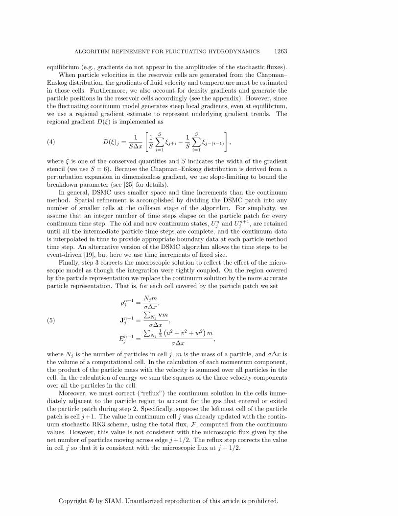
Finally, step 3 corrects the macroscopic solution to reflect the effect of the micro-scopic model as though the integration were tightly coupled. On the region coveredby the particle representation we replace the continuum solution by the more accurateparticle representation. That is, for each cell covered by the particle patch we set
ρn+1j =
Njm
σΔx,
Jn+1j =
∑Nj
vm
σΔx,(5)
En+1j =
∑Nj
12
(u2 + v2 + w2
)m
σΔx,
where Nj is the number of particles in cell j, m is the mass of a particle, and σΔx isthe volume of a computational cell. In the calculation of each momentum component,the product of the particle mass with the velocity is summed over all particles in thecell. In the calculation of energy we sum the squares of the three velocity componentsover all the particles in the cell.
Moreover, we must correct (“reflux”) the continuum solution in the cells imme-diately adjacent to the particle region to account for the gas that entered or exitedthe particle patch during step 2. Specifically, suppose the leftmost cell of the particlepatch is cell j+1. The value in continuum cell j was already updated with the contin-uum stochastic RK3 scheme, using the total flux, F , computed from the continuumvalues. However, this value is not consistent with the microscopic flux given by thenet number of particles moving across edge j+1/2. The reflux step corrects the valuein cell j so that it is consistent with the microscopic flux at j + 1/2.
To perform the refluxing correction we monitor the number of particles, N→j+1/2
and N←j+1/2, that move into and out of the particle region, respectively, across the
continuum/particle interface at edge j + 1/2. We then correct the continuum solu-tion as
(6) U′n+1j = Un+1
j +Δt
Δx(FΣ
j+1/2 −FPj+1/2),
where the prime indicates the value after the refluxing update. The net particle flux is
(7) FPj+1/2 =
m
σΔt
⎛⎝ N→
j+1/2 −N←j+1/2∑→
i vi −∑←
i vi12
∑→i |vi|2 − 1
2
∑←i |vi|2
⎞⎠ ,
where∑→
i and∑←
i are sums over particles crossing the interface from left to rightand right to left, respectively.
This update effectively replaces the continuum flux component of the update toUn+1j on edge j+1/2 by the flux of particles with their associated momentum through
the edge. An analogous refluxing step occurs in the cell adjacent to the right-handboundary of the particle region. Finally, note that this synchronization procedureguarantees conservation. The technical details of refluxing in higher dimensions (e.g.,the treatment of corners) are discussed in Garcia et al. [26].
4. Numerical results. This section presents a series of computational exam-ples, of progressively increasing sophistication, that demonstrate the accuracy andeffectiveness of the algorithm refinement hybrid. First we examine an equilibriumsystem, then several nonequilibrium examples, concluding with a demonstration ofadaptive refinement.
In our testing we compare three numerical schemes: the stochastic scheme basedon three-stage Runge–Kutta for the LLNS equations discussed in section 2.1 (stoch.PDE only) and two algorithm refinement hybrids as described in section 3. Thefirst hybrid couples DSMC and stochastic RK3 (stoch. hybrid). The second hybridis similar but without a stochastic flux in the LLNS equations; that is, it uses adeterministic version of RK3 (deter. hybrid). In some of the tests the results fromthese schemes are compared with data from a pure DSMC calculation.
The parameters used in the various numerical tests were selected, when possible,to be the same as in [7] to allow for comparison. In that paper it was establishedthat the stochastic RK3 method had a linear convergence of variances in both Δxand Δt and was accurate to within a few percentage points for parameters used here.Furthermore, simulation parameters were chosen to be typical for a DSMC simulation.For example, the time step and cell size truncation errors in DSMC dictate that anaccurate simulation requires these to be a fraction of a mean collision time and a meanfree path, respectively [11]. The cell volume was selected such that the amplitude ofthe fluctuations was significant (with a standard deviation of about 10% of the mean)while remaining within the range of validity of fluctuating hydrodynamics.
In principle, the continuum grid of an AMAR hybrid may have as many hier-archical levels as necessary, and there may be many disjoint and/or linked DSMCpatches. For simplicity, here we will consider a single DSMC region embedded withina single-level continuum grid. Furthermore, in the following numerical examples weuse equal mesh spacing, Δx, and time step size, Δt, in both the continuum and par-ticle methods. The straightforward adjustments necessary for implementing a DSMCgrid with smaller Δx and Δt are presented in section 3.
Number of computational cells 40Cell length (Δx) 3.13 × 10⁻⁶
Time step (Δt) 1.0 × 10⁻¹²
4.1. Equilibrium system: State variables. First, we consider a system ina periodic domain with zero bulk flow and uniform mean energy and mass density.Parameters for this equilibrium system are given in Table 1. Results from this firsttest problem are depicted in Figures 2–5. For both algorithm refinement hybrids, theparticle patch is fixed at the center of the domain, covering cells 15–24, indicated inthe figures by vertical dotted black lines. For this equilibrium problem the particles inthe patches used to provide boundary reservoirs for DSMC have velocities generatedfrom the Maxwell–Boltzmann distribution. In each simulation the system is initializednear the final state and is allowed to relax for 5 × 10⁶ time steps. Statistics are thengathered over 107 time steps. Note that in these first tests we confirmed that all threeschemes conserve total density, momentum, and energy; recall that the hybrids areconservative due to the “refluxing” step.1
First, we examine mass density; results from the various numerical schemes areshown in Figure 2. The first panel shows the mean of mass density at each spatiallocation, 〈ρi〉, and the second panel shows the variance, 〈δρ2
i 〉 = 〈(ρi − 〈ρi〉)2〉. Thethird panel shows the center-point correlation, 〈δρiδρj=20〉, that is, the covariance ofδρi with the value at the center of the domain (j = 20). These three quantities areestimated from samples as
〈ρi〉 =1
Ns
Ns∑n=1
ρni ,
〈δρ2i 〉 =
(1
Ns
Ns∑n=1
(ρni )2
)− 〈ρi〉2,
〈δρiδρ20〉 =
(1
Ns
Ns∑n=1
ρni ρn20
)− 〈ρi〉〈ρ20〉,
1When the grids move dynamically, this exact conservation is lost because of quantization effectsassociated with initialization of a particle distribution from continuum data.
Fig. 2. Mean, variance, and center-point correlation of mass density versus spatial location fora system at equilibrium. Vertical dotted lines depict the boundaries of the particle region for bothhybrids. Note that, for clarity, the correlation value at i = j = 20 is omitted from the plot.
where Ns = 107 is the number of samples and i = 1, . . . , 40. Similar statistics for x-momentum, y-momentum, and energy are displayed in Figures 3 and 5; the statisticsfor z-momentum are similar to those for y-momentum and are omitted here. Weconsider only these conserved mechanical variables because the continuum schemeis based on them, they are easily measured in molecular simulations, and hydrody-namic variables, such as pressure and temperature, are directly obtained from thesemechanical variables [24].
We obtain the correct mean values for all three schemes, with the continuummethod exhibiting some numerical oscillations, most notably in the x-momentum.For the most part, the correct variance values are also obtained by the two stochasticschemes. In fact, the stochastic continuum method used here was developed in [7]with the particular goal of correctly reproducing the variances of conserved quantities.Nevertheless, some localized errors in variance introduced by the stochastic hybridalgorithm are evident in these figures. At the left and right boundaries of the particlepatch, there is a peak error in the variance of about 23% for mass density and 14% forenergy. These discrepancies are discussed in detail in section 4.2.
Figures 2–5 also illustrate the effect on fluctuations when the hybrid’s continuumPDE scheme does not include a stochastic flux. Clearly, the variances drop to near zeroinside the deterministic continuum regions, left and right of the particle patch. Moresignificantly, the variances within the patch are also damped. Even more interestingis the appearance of a large correlation of fluctuations in the particle region of the
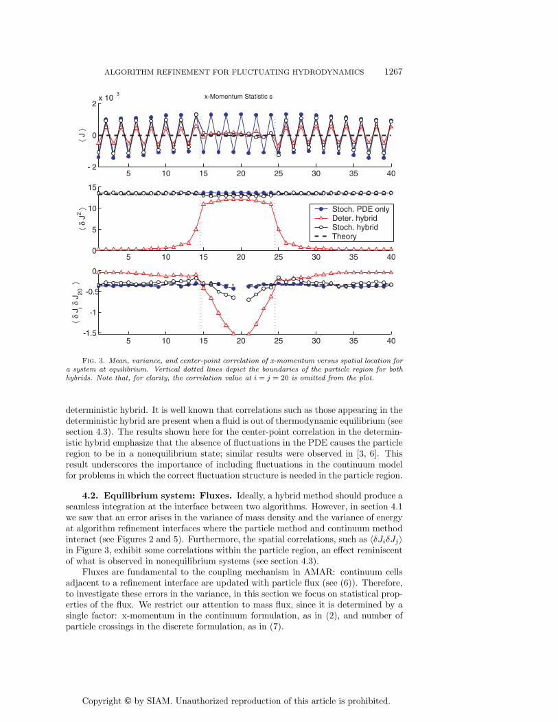
Fig. 3. Mean, variance, and center-point correlation of x-momentum versus spatial location fora system at equilibrium. Vertical dotted lines depict the boundaries of the particle region for bothhybrids. Note that, for clarity, the correlation value at i = j = 20 is omitted from the plot.
deterministic hybrid. It is well known that correlations such as those appearing in thedeterministic hybrid are present when a fluid is out of thermodynamic equilibrium (seesection 4.3). The results shown here for the center-point correlation in the determin-istic hybrid emphasize that the absence of fluctuations in the PDE causes the particleregion to be in a nonequilibrium state; similar results were observed in [3, 6]. Thisresult underscores the importance of including fluctuations in the continuum modelfor problems in which the correct fluctuation structure is needed in the particle region.
4.2. Equilibrium system: Fluxes. Ideally, a hybrid method should produce aseamless integration at the interface between two algorithms. However, in section 4.1we saw that an error arises in the variance of mass density and the variance of energyat algorithm refinement interfaces where the particle method and continuum methodinteract (see Figures 2 and 5). Furthermore, the spatial correlations, such as 〈δJiδJj〉in Figure 3, exhibit some correlations within the particle region, an effect reminiscentof what is observed in nonequilibrium systems (see section 4.3).
Fluxes are fundamental to the coupling mechanism in AMAR: continuum cellsadjacent to a refinement interface are updated with particle flux (see (6)). Therefore,to investigate these errors in the variance, in this section we focus on statistical prop-erties of the flux. We restrict our attention to mass flux, since it is determined by asingle factor: x-momentum in the continuum formulation, as in (2), and number ofparticle crossings in the discrete formulation, as in (7).
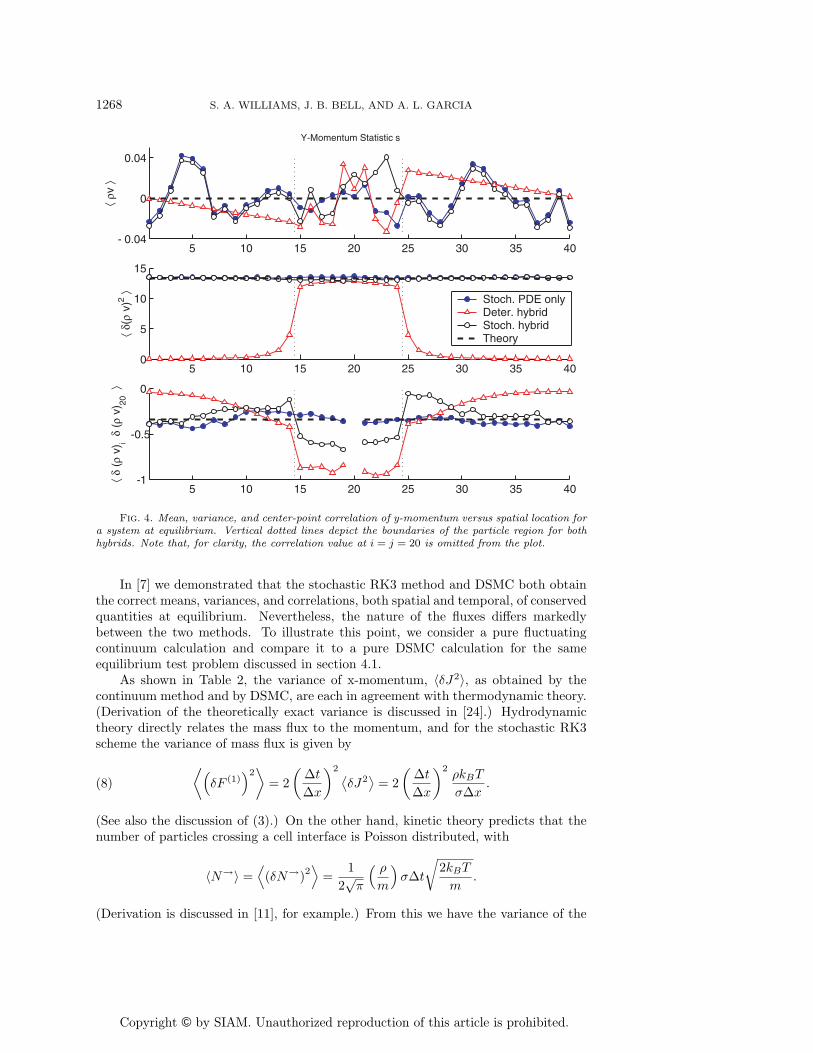
Fig. 4. Mean, variance, and center-point correlation of y-momentum versus spatial location fora system at equilibrium. Vertical dotted lines depict the boundaries of the particle region for bothhybrids. Note that, for clarity, the correlation value at i = j = 20 is omitted from the plot.
In [7] we demonstrated that the stochastic RK3 method and DSMC both obtainthe correct means, variances, and correlations, both spatial and temporal, of conservedquantities at equilibrium. Nevertheless, the nature of the fluxes differs markedlybetween the two methods. To illustrate this point, we consider a pure fluctuatingcontinuum calculation and compare it to a pure DSMC calculation for the sameequilibrium test problem discussed in section 4.1.
As shown in Table 2, the variance of x-momentum, 〈δJ2〉, as obtained by thecontinuum method and by DSMC, are each in agreement with thermodynamic theory.(Derivation of the theoretically exact variance is discussed in [24].) Hydrodynamictheory directly relates the mass flux to the momentum, and for the stochastic RK3scheme the variance of mass flux is given by
(8)
⟨(δF (1)
)2⟩
= 2
(Δt
Δx
)2 ⟨δJ2
⟩= 2
(Δt
Δx
)2ρkBT
σΔx.
(See also the discussion of (3).) On the other hand, kinetic theory predicts that thenumber of particles crossing a cell interface is Poisson distributed, with
〈N→〉 =⟨(δN→)
2⟩
=1
2√π
( ρ
m
)σΔt
√2kBT
m.
(Derivation is discussed in [11], for example.) From this we have the variance of the
Fig. 5. Mean, variance, and center-point correlation of energy versus spatial location for asystem at equilibrium. Vertical dotted lines depict the boundaries of the particle region for bothhybrids. Note that, for clarity, the correlation value at i = j = 20 is omitted from the plot.
Table 2
Variance of x-momentum and of mass flux at equilibrium.
〈δJ2〉 〈δF (1)2 〉Stoch. PDEonly
DSMC Stoch. PDEonly
DSMC
Computed value 13.62 13.21 2.84E-12 1.44E-10Thermodynamic theory 13.34 13.34Hydrodynamic theory 2.72E-12Kinetic theory 1.46E-10Percentage error 2.1% -1.0% 4.3% -1.8%
mass flux given by⟨(δF (1)
)2⟩
=m2
(σΔx)2
⟨δ (N→ −N←)
2⟩
=2m2
(σΔx)2
⟨(δN→)
2⟩
=mρ√π σ
Δt
Δx2
√2kBT
m.(9)
Comparing (8) and (9), one finds that the hydrodynamic and kinetic theory expres-sions match when the Courant number, C = cΔt/Δx, is order one, yet for the runspresented here C ≈ 10−2 (see Table 1).
From Table 2, we see that the variance of the mass flux for the continuum methodis in good agreement with the hydrodynamic theory (see (8)), and the corresponding
Values at t’ = 0 are not shown.DSMC value: 1.4365e−10PDE value: 2.8412e−12
DSMCStoch. PDE only
Fig. 6. Time correlations of mass flux for the particle method (DSMC) and the PDE method.
DSMC result is in good agreement with kinetic theory (see (9)). Yet, the two variancesof mass flux differ by over two orders of magnitude. To understand the nature of thisdiscrepancy, we investigate the time correlation of the mass flux.
To estimate the time correlation of mass flux for a timeshift of t′, we calcu-late 〈δF (1)(t)δF (1)(t + t′)〉 in each of the 40 computational cells from approximately105 data samples. The average value of each time correlation over the 40 computa-tional cells is displayed in Figure 6 for stochastic RK3 and for DSMC. Time correlationdata is displayed in units of mean free collision time (tm).
In Figure 6 we see that the mass flux for DSMC decorrelates immediately, whereasthe continuum mass flux decorrelates after approximately one half of one mean freecollision time. Note that for all the simulation results presented here, the stochasticPDE and the DSMC use the same time step, and that time step is over two ordersof magnitude smaller than tm. The origin of the discrepancy in Table 2 is nowclear. The hydrodynamic formulation is accurate only at hydrodynamic time scales,that is, at time scales that are large compared to tm. Further investigations (notpresented here) indicate that when the two methods are run using a significantlylarger time step, the variance and time correlations of the mass flux are in generalagreement between the two methods. However, at large time step, the truncationerror for the PDE scheme negatively affects the results for other quantities, e.g., thevariance in conserved quantities. Given that the statistical properties of the fluxesdiffer between hydrodynamic scales and molecular (kinetic) scales, it is not surprising
ALGORITHM REFINEMENT FOR FLUCTUATING HYDRODYNAMICS 1271
5 10 15 20 25 30 35 40−2.5
−2
−1.5
−1
−0.5
0
0.5
1
1.5
x 10−5
⟨ δ ρ
i δ J
20 ⟩
DSMCStoch. PDE only
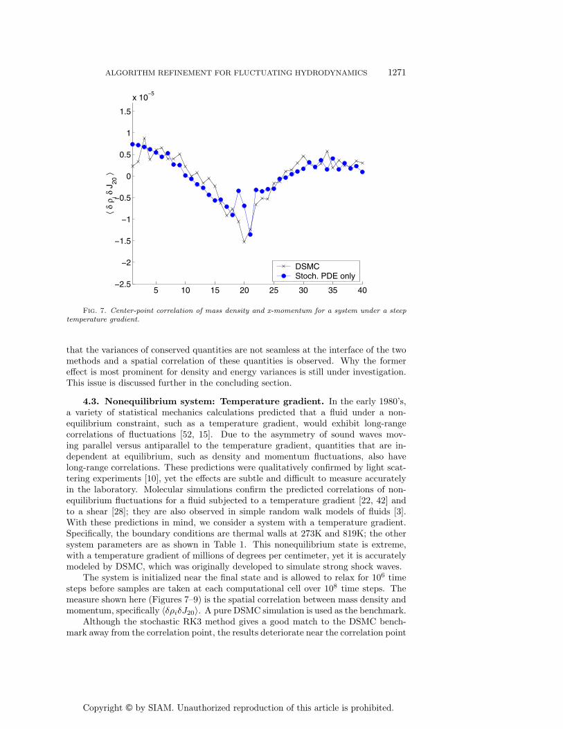
Fig. 7. Center-point correlation of mass density and x-momentum for a system under a steeptemperature gradient.
that the variances of conserved quantities are not seamless at the interface of the twomethods and a spatial correlation of these quantities is observed. Why the formereffect is most prominent for density and energy variances is still under investigation.This issue is discussed further in the concluding section.
4.3. Nonequilibrium system: Temperature gradient. In the early 1980’s,a variety of statistical mechanics calculations predicted that a fluid under a non-equilibrium constraint, such as a temperature gradient, would exhibit long-rangecorrelations of fluctuations [52, 15]. Due to the asymmetry of sound waves mov-ing parallel versus antiparallel to the temperature gradient, quantities that are in-dependent at equilibrium, such as density and momentum fluctuations, also havelong-range correlations. These predictions were qualitatively confirmed by light scat-tering experiments [10], yet the effects are subtle and difficult to measure accuratelyin the laboratory. Molecular simulations confirm the predicted correlations of non-equilibrium fluctuations for a fluid subjected to a temperature gradient [22, 42] andto a shear [28]; they are also observed in simple random walk models of fluids [3].With these predictions in mind, we consider a system with a temperature gradient.Specifically, the boundary conditions are thermal walls at 273K and 819K; the othersystem parameters are as shown in Table 1. This nonequilibrium state is extreme,with a temperature gradient of millions of degrees per centimeter, yet it is accuratelymodeled by DSMC, which was originally developed to simulate strong shock waves.
The system is initialized near the final state and is allowed to relax for 106 timesteps before samples are taken at each computational cell over 108 time steps. Themeasure shown here (Figures 7–9) is the spatial correlation between mass density andmomentum, specifically 〈δρiδJ20〉. A pure DSMC simulation is used as the benchmark.
Although the stochastic RK3 method gives a good match to the DSMC bench-mark away from the correlation point, the results deteriorate near the correlation point
Fig. 8. Center-point correlation of mass density and x-momentum for a system under a steeptemperature gradient. Vertical dotted lines depict the boundaries of the particle region for the hybridmethod.
5 10 15 20 25 30 35 40 -2.5
-2
-1.5
-1
-0.5
0
0.5
1
1.5
x 10- 5
⟨ δ ρ
i δ J
20 ⟩
DSMCDeter. hybridRefinement region
Fig. 9. Center-point correlation of mass density and x-momentum for a system under a steeptemperature gradient. Vertical dotted lines depict the boundaries of the particle region for the hybridmethod.
(Figure 7). In the stochastic hybrid method, a particle patch is placed around theregion of difficulty, and the results are significantly improved in that region (Figure 8).Given that theoretical results often make predictions for the near–center-point
correlations (e.g., 〈δρiδJj〉 ∝ ∇T for i ≈ j), making it the region of interest, thestochastic hybrid method outperforms the pure continuum method in this nonequi-librium test case. Finally, in Figure 9 we consider the hybrid that couples deterministicRK3 with DSMC. Again, DSMC is employed in a single patch at the center of thedomain. However, with fluctuations suppressed in the remainder of the domain, theoverall results suffer. Strikingly, the results suffer not only in the continuum regionbut also within the particle region.
4.4. Nonequilibrium system: Strong moving shock. In this time-depen-dent problem, we consider a Mach 2 shock traveling through a domain that includes astatic refinement region. The objective of this example is to test how well the hybridperforms when a strong nonlinear wave crosses the interface between continuum andparticle regions. Dirichlet boundary conditions are used at the domain boundaries;values for the left-hand state (LHS) and right-hand state (RHS) are given in Table 3.
The mass density profile depicted by the dark line is an average profile from anensemble of 2000 stochastic hybrid runs. Results from an ensemble of 2000 purestochastic PDE simulations of the traveling wave, without a particle patch, are shownfor comparison. The first panel of Figure 10 also includes the mass density profilefrom a single stochastic hybrid simulation, illustrating the relative magnitude of thethermal fluctuations. At time t0, before the shock enters the particle region, theensemble-averaged data is smooth. At time t1, a spurious reflected wave is formed atthe interface on the left-hand side of the particle patch. This spurious acoustic waveis damped as it propagates leftward, vanishing by time t4. Another small error effectis seen as the shock exits the particle patch, at time t5, but it is barely discernible bytime t7. In summary, we observe a relatively local and short-lived error that indicatesan impedance mismatch between the continuum and particle regions, as shown inFigure 10. This mismatch is likely due to the linear approximation of the shear stressand heat flux in the Navier–Stokes equations, which is not accurate for the steepgradients of a strong shock. More complicated expressions for the dissipative fluxeshave been derived (e.g., Burnett equations [14]), but for a variety of reasons, such asdifficulties in treating boundary conditions, they are not in common use in CFD.
A well-known feature of CFD solvers is the artificial steepening of viscous shockprofiles; it is also well established that DSMC predicts shock profiles accurately [11, 4].At times t2 through t6, we see a steepness discrepancy between the ensemble hybridprofile and the ensemble PDE-only profile. Within the particle patch, the DSMCalgorithm correctly resolves a more shallow profile. This example demonstrates therobustness and stability of the treatment of the interface between the particle regionand the continuum solver.
Ensemble of stochastic PDE runsEnsemble of stochastic hybrid runsSingle stochastic hybrid run
t1
t2
t3
t4
t5
t6
t7
10 20 30 40 50 60 70
t8
Fig. 10. Mass density profiles for a viscous shock wave traveling through a fixed refinementregion (indicated by vertical dotted lines). The time elapsed between each panel is 300Δt; see Table 3for system parameters.
ALGORITHM REFINEMENT FOR FLUCTUATING HYDRODYNAMICS 1275
t0
Ensemble of stochastic PDE runsEnsemble of stochastic hybrid runsSingle stochastic hybrid run
t1
t2
25 50 75 100 125
t3
Fig. 11. Mass density profiles for a viscous shock wave, demonstrating AMR: The refinementregion, indicated by vertical dotted lines, is determined dynamically at runtime. The time elapsedbetween each panel is 1200Δt; see Table 3 for system parameters.
Finally, in this example, the Chapman–Enskog distribution was used to initializevelocities of particles that enter the refinement region from the continuum region. Thisapproach was found to result in a somewhat reduced impedance mismatch comparedto the Maxwell–Boltzmann distribution.
4.5. Adaptive refinement. The final numerical test demonstrates the adaptiverefinement capability of our hybrid algorithm. As in section 4.4, a strong travelingshock (Mach 2) moves through a domain with Dirichlet boundary conditions; systemparameters are given in Table 3. Here, though, the location of a particle patch isdetermined dynamically by identifying cells in which the gradient of pressure exceedsa given tolerance; the particle patch is shown in Figure 11 by vertical dotted lines.
Large scale gradients in pressure provide an effective criterion for identifying thepresence of a shock wave. Since the fluctuations produce steep localized gradientsnearly everywhere, a regional gradient measure, D(P ), is employed to detect thesestrong gradients. This is implemented as
D(P )j =1
SΔx
[1
S
S∑i=1
Pj+i −1
S
S∑i=1
Pj−(i−1)
],
where S indicates the width of the gradient stencil (we use S = 6). For an equilibriumsystem, the expected variance of D(P ) is estimated by
where ρ0, T0, and P0 are the reference mass density, temperature, and pressure forthe system and Nc is the number of particles in a cell at reference conditions. (Thisvariance can be found using the ideal gas law and expressions derived in [24].) Notethat using a wide stencil limits the variation even when Nc is small (and, consequently,fluctuations are large). We select cells j for refinement where D(P )j exceeds theequilibrium value, namely zero, by three standard deviations. The resulting particlepatch is extended by a buffer of four cells on each side.
In this implementation, we re-evaluate the location of the particle patch every100 time steps. When the extent of the refinement region changes, some continuumcells may be added to the DSMC patch, some DSMC cells may become continuumcells, and some DSMC cells may remain in the refinement patch. For continuumcells that are added to the DSMC patch, particles are initialized from the underlyingcontinuum data, as in the case of a static patch. For DSMC cells that should no longerbe included in the refinement patch, particle data is averaged onto the continuum grid,as in (5), then discarded. For those DSMC cells that remain in the particle patch,the particle data is retained.
The mass density profile depicted by the dark line is an average profile from anensemble of 2000 stochastic hybrid runs. The first panel of Figure 11 also includesthe mass density profile from a single stochastic hybrid simulation, illustrating therelative magnitude of the thermal fluctuations. Results from an ensemble of 2000pure stochastic PDE simulations of the traveling wave, without a particle patch, arealso shown for comparison. As in Figure 10, we show that a more shallow profile iscaptured by the DSMC representation of the viscous shock (i.e., by the hybrid thatuses DSMC in the vicinity of the shock) versus the artificially steep profile producedby the PDE-only system.
5. Conclusions and further work. We have constructed a hybrid algorithmthat couples a DSMC molecular simulation with a new numerical solver for the LLNSequations for fluctuating compressible flow. The algorithm allows the particle methodto be used locally to approximate the solution while modeling the system using themean field equations in the remainder of the domain. In tests of the method we havedemonstrated that it is necessary to include the effect of fluctuations, represented asa stochastic flux, in the mean field equations to ensure that the hybrid preserved keyproperties of the system. As expected, not representing fluctuations in the continuumregime leads to a decay in the variance of the solution that penetrates into the particleregion. Somewhat more surprising is that the failure to include fluctuations was shownto introduce spurious correlations of fluctuations in equilibrium simulations.
The coupling of the particle and continuum algorithms presented here is notentirely seamless for the variance and correlations of conserved quantities. The mis-match appears to be primarily caused by the inability of the continuum stochasticPDE to reproduce the temporal spectrum of the particle fluxes at kinetic time scales.This is not so much a failure of the methodology as much as a fundamental differencebetween molecular and hydrodynamic scales. With this caveat, one still finds thatusing a stochastic PDE in an AMAR hybrid yields significantly better fidelity in thefluctuation variances and correlations, making it useful for applications such as thosedescribed in the introduction.
There are several directions that we plan to pursue in future work. As a first step,we plan to extend the methodology to two- and three-dimensional hybrids. The keyalgorithmic steps developed here extend naturally to multiple dimensions. For moregeneral applications, an overall approach needs to be implemented to support particle
ALGORITHM REFINEMENT FOR FLUCTUATING HYDRODYNAMICS 1277
regions defined by a union of nonoverlapping patches. Another area of development isto include additional physical effects in both the continuum and particle models. Asa first step in this direction, it is straightforward to include the capability to modeldifferent species. This provides the necessary functionality needed to study Rayleigh–Taylor instabilities and other mixing phenomena. A longer term goal along theselines would be to include chemical reactions within the model to enable the studyof ignition phenomena. Finally, we note that the results presented here suggest anumber of potential improvements to the core methodology. Of particular interestin this area would be approaches to the fluctuating continuum equations that canaccurately capture fluctuations while taking a larger time step. This would not onlyimprove the efficiency of the methodology, it would also enable the continuum solverto take time steps at hydrodynamic time scales which should serve to improve thequality of coupling between continuum and particle regions.
Appendix. Random placement of particles with a density gradient.Consider the problem of selecting a random position for a particle within a rectangularcell. The density in the cell varies linearly with ρ0 being the density at the center(which is also the mean density). For a cell with dimensions Δx, Δy, and Δz, takingthe origin at the corner of the cell we have
where ax = ∂ρ/∂x. The probability that a particle has position component x is
P (x) =
∫ Δy
0dy
∫ Δz
0dz ρ(x, y, z)
ρ0ΔxΔyΔz=
1 + γx(x/Δx− 12 )
Δx,
where γx ≡ Δxax/ρ0. It will be more convenient to work in the dimensionless variableX = x/Δx. Since P (x) dx = P (X) dX,
P (X) = 1 + γx
(X − 1
2
).
By the method of inversion [23] one may generate random values from this distribu-tion by
X = γ−1x
[(γx/2 − 1) +
[(γx/2 − 1)2 + 2γxR
]1/2],
where R is a random value uniformly distributed in [0, 1]. The reader is cautionedthat the above is susceptible to round-off error for γx ≈ 0 (i.e., small gradient case).Note that in that limit,
X ≈ R1 − γx/2
,
from which we recover the expected result that X = R when γx = 0.The selection of the y component of the position is complicated by the fact that
it is not independent of the x component. The conditional probability of the y com-ponent of position is
Fortunately, after selecting X the selection of Y is simple; Y is generated in the sameway as X but with γy/P (X) in place of γx.
Finally, to select the z component of the position the procedure is similar to
P (Z|X,Y ) = 1 +γz
P (X,Y )
(Z − 1
2
),
where P (X,Y ) = P (X|Y )P (Y ) = 1 + γx(X − 12 ) + γy(Y − 1
2 ). Again, the z com-ponent can be generated in the same way as the x component but with γz/P (X,Y )replacing γx.
REFERENCES
[1] F. J. Alexander and A. L. Garcia, The direct simulation Monte Carlo method, Computersin Physics, 11 (1997), pp. 588–593.
[2] F. J. Alexander, A. L. Garcia, and D. M. Tartakovsky, Algorithm refinement for sto-chastic partial differential equations: I. Linear diffusion, J. Comput. Phys., 182 (2002),pp. 47–66.
[3] F. J. Alexander, A. L. Garcia, and D. M. Tartakovsky, Algorithm refinement for stochas-tic partial differential equations: II. Correlated systems, J. Comput. Phys., 207 (2005), pp.769–787.
[4] H. Alsmeyer, Density profiles in argon and nitrogen shock waves measured by the absorptionof an electron beam, J. Fluid Mech., 74 (1976), pp. 497–513.
[5] J. B. Bell, M. Berger, J. Saltzman, and M. Welcome, Three-dimensional adaptive meshrefinement for hyperbolic conservation law, SIAM J. Sci. Comput., 15 (1994), pp. 127–138.
[6] J. B. Bell, J. Foo, and A. Garcia, Algorithm refinement for the stochastic Burgers’ equation,J. Comput. Phys., 223 (2007), pp. 451–468.
[7] J. B. Bell, A. L. Garcia, and S. A. Williams, Numerical methods for the stochastic Landau-Lifshitz Navier-Stokes equations, Phys. Rev. E (3), 76 (2007), 016708.
[8] M. Berger and P. Colella, Local adaptive mesh refinement for shock hydrodynamics, J.Comput. Phys., 82 (1989), pp. 64–84.
[9] M. Berger and J. Oliger, Adaptive mesh refinement for hyperbolic partial differential equa-tions, J. Comput. Phys., 53 (1984), pp. 484–512.
[10] D. Beysens, Y. Garrabos, and G. Zalczer, Experimental evidence for Brillouin asymmetryinduced by a temperature gradient, Phys. Rev. Lett., 45 (1980), pp. 403–406.
[11] G. A. Bird, Molecular Gas Dynamics and the Direct Simulation of Gas Flows, Clarendon,Oxford, UK, 1994.
[12] M. Bixon and R. Zwanzig, Boltzmann-Langevin equation and hydrodynamic fluctuations,Phys. Rev., 187 (1969), pp. 267–272.
[14] S. Chapman and T. G. Cowling, The Mathematical Theory of Non-Uniform Gases, Cam-bridge University Press, Cambridge, UK, 1991.
[15] J. M. Ortiz de Zarate and J. V. Sengers, Hydrodynamic Fluctuations in Fluids and FluidMixtures, Elsevier Science, Amsterdam, 2007.
[16] R. Delgado-Buscalioni and P. V. Coveney, Continuum-particle hybrid coupling for mass,momentum, and energy transfers in unsteady fluid flow, Phys. Rev. E (3), 67 (2003),046704.
[17] R. Delgado-Buscalioni and G. De Fabritiis, Embedding molecular dynamics within fluc-tuating hydrodynamics in multiscale simulations of liquids, Phys. Rev. E (3), 76 (2007),036709.
[18] C. Van den Broeck, R. Kawai, and P. Meurs, Exorcising a Maxwell demon, Phys. Rev.Lett., 93 (2004), 090601.
[19] A. Donev, A. L. Garcia, and B. J. Alder, Stochastic event-driven molecular dynamics, J.Comput. Phys., 227 (2007), pp. 2644–2665.
ALGORITHM REFINEMENT FOR FLUCTUATING HYDRODYNAMICS 1279
[20] J. Eggers, Dynamics of liquid nanojets, Phys. Rev. Lett., 89 (2002), 084502.[21] R. F. Fox and G. E. Uhlenbeck, Contributions to non-equilibrium thermodynamics. I. Theory
of hydrodynamical fluctuations, Phys. Fluids, 13 (1970), pp. 1893–1902.[22] A. L. Garcia, Nonequilibrium fluctuations studied by a rarefied gas simulation, Phys. Rev. A,
34 (1986), pp. 1454–1457.[23] A. L. Garcia, Numerical Methods for Physics, 2nd ed., Prentice Hall, Englewood Cliffs, NJ,
2000.[24] A. L. Garcia, Estimating hydrodynamic quantities in the presence of microscopic fluctuations,
Commun. Appl. Math. Comput. Sci., 1 (2006), pp. 53–78.[25] A. L. Garcia and B. J. Alder, Generation of the Chapman-Enskog distribution, J. Comput.
Phys., 140 (1998), pp. 66–70.[26] A. L. Garcia, J. B. Bell, W. Y. Crutchfield, and B. J. Alder, Adaptive mesh and algo-
rithm refinement using direct simulation Monte Carlo, J. Comput. Phys., 154 (1999), pp.134–155.
[27] A. L. Garcia, M. Malek-Mansour, G. Lie, and E. Clementi, Numerical integration of thefluctuating hydrodynamic equations, J. Statist. Phys., 47 (1987), p. 209.
[28] A. L. Garcia, M. Malek-Mansour, G. C. Lie, M. Mareschal, and E. Clementi, Hydro-dynamic fluctuations in a dilute gas under shear, Phys. Rev. A, 36 (1987), pp. 4348–4355.
[29] A. L. Garcia and C. Penland, Fluctuating hydrodynamics and principal oscillation patternanalysis, J. Statist. Phys., 64 (1991), pp. 1121–1132.
[30] G. Giupponi, G. De Fabritiis, and P. V. Coveney, Hybrid method coupling fluctuatinghydrodynamics and molecular dynamics for the simulation of macromolecules, J. ChemicalPhysics, 126 (2007), 154903.
[31] S. Gottleib and C. Shu, Total variation diminishing Runge-Kutta schemes, Math. Comp.,67 (1998), pp. 73–85.
[32] N. G. Hadjiconstantinou, Discussion of recent developments in hybrid atomistic-continuummethods for multiscale hydrodynamics, Bull. Polish Acad. Sci. Tech. Sci., 53 (2005), pp.335–342.
[33] R. D. Astumian and P. Hanggi, Brownian motors, Physics Today, 55 (2002), pp. 33–39.[34] M. Kac, Foundations of kinetic theory, in Proceedings of the 3rd Berkeley Symposium on
Math. Statist. Probab. Vol. 3, J. Neyman, ed., University of California Press, Berkeley,CA, 1954, pp. 171–197.
[35] K. Kadau, T. C. Germann, N. G. Hadjiconstantinou, P. S. Lomdahl, G. Dimonte, B. L.
Holian, and B. J. Alder, Nanohydrodynamics simulations: An atomistic view of theRayleigh-Taylor instability, Proc. Natl. Acad. Sci. USA, 101 (2004), pp. 5851–5855.
[36] K. Kadau, C. Rosenblatt, J. L. Barber, T. C. Germann, Z. Huang, P. Carls, and B. J.
Alder, The importance of fluctuations in fluid mixing, Proc. Natl. Acad. Sci. USA, 104(2007), pp. 7741–7745.
[37] W. Kang and U. Landman, Universality crossover of the pinch-off shape profiles of collapsingliquid nanobridges in vacuum and gaseous environments, Phys. Rev. Lett., 98 (2007),064504.
[38] G. E. Kelly and M. B. Lewis, Hydrodynamic fluctuations, Phys. Fluids, 14 (1971), pp. 1925–1931.
[39] V. I. Kolobov, R. R. Arslanbekov, V. V. Aristov, A. A. Frolova, and S. A. Zabe-
lok, Unified solver for rarefied and continuum flows with adaptive mesh and algorithmrefinement, J. Comput. Phys., 223 (2007), pp. 589–608.
[40] L. D. Landau and E. M. Lifshitz, Fluid Mechanics, Course of Theoretical Physics 6, Perga-mon, London, 1959.
[41] A. Lemarchand and B. Nowakowski, Fluctuation-induced and nonequilibrium-induced bifur-cations in a thermochemical system, Molecular Simulation, 30 (2004), pp. 773–780.
[42] M. Malek-Mansour, A. L. Garcia, G. C. Lie, and E. Clementi, Fluctuating hydrodynamicsin a dilute gas, Phys. Rev. Lett., 58 (1987), pp. 874–877.
[43] M. Malek-Mansour, A. L. Garcia, J. W. Turner, and M. Mareschal, On the scatteringfunction of simple fluids in finite systems, J. Statist. Phys., 52 (1988), pp. 295–309.
[44] M. Mareschal, M. Malek-Mansour, G. Sonnino, and E. Kestemont, Dynamic structurefactor in a nonequilibrium fluid: A molecular-dynamics approach, Phys. Rev. A, 45 (1992),pp. 7180–7183.
[45] P. Meurs, C. Van den Broeck, and A. L. Garcia, Rectification of thermal fluctuations inideal gases, Phys. Rev. E (3), 70 (2004), 051109.
[46] E. Moro, Hybrid method for simulating front propagation in reaction-diffusion systems, Phys.Rev. E (3), 69 (2004), 060101.
[47] M. Moseler and U. Landman, Formation, stability, and breakup of nanojets, Science, 289(2000), pp. 1165–1169.
[48] P. Espanol, Stochastic differential equations for non-linear hydrodynamics, Phys. A, 248(1998), pp. 77–96.
[49] B. Nowakowski and A. Lemarchand, Sensitivity of explosion to departure from partial equi-librium, Phys. Rev. E, 68 (2003), 031105.
[50] G. Oster, Brownian ratchets: Darwin’s motors, Nature, 417 (2002), p. 25.[51] J. Qiu and C.-W. Shu, Runge–Kutta discontinuous Galerkin method using WENO limiters,
SIAM J. Sci. Comput., 26 (2005), pp. 907–929.[52] R. Schmitz, Fluctuations in nonequilibrium fluids, Phys. Rep., 171 (1988), pp. 1–58.[53] T. E. Schwarzentruber, L. C. Scalabrin, and I. D. Boyd, A modular particle-continuum
numerical method for hypersonic non-equilibrium gas flows, J. Comput. Phys., 225 (2007),pp. 1159–1174.
[54] W. Wagner, A convergence proof for Bird’s direct simulation Monte Carlo method for theBoltzmann equation, J. Statist. Phys., 66 (1992), pp. 1011–1044.
[55] H. S. Wijesinghe and N. G. Hadjiconstantinou, Discussion of hybrid atomistic-continuummethods for multiscale hydrodynamics, Internat. J. Multiscale Computational Engineering,2 (2004), pp. 189–202.
[56] H. S. Wijesinghe, R. Hornung, A. L. Garcia, and N. G. Hadjiconstantinou, Three-dimensional hybrid continuum-atomistic simulations for multiscale hydrodynamics, J. Flu-ids Eng., 126 (2004), pp. 768–777.