83
i Mohammad Abdullah Abu Diyan MULTI-SCALE VEGETATION CLASSIFICATION USING EARTH OBSERVATION DATA OF THE SUNDARBAN MANGROVE FOREST, BANGLADESH
i
Mohammad Abdullah Abu Diyan
MULTI-SCALE VEGETATION CLASSIFICATION USING EARTH OBSERVATION DATA OF THE SUNDARBAN MANGROVE FOREST, BANGLADESH

ii
MULTI-SCALE VEGETATION CLASSIFICATION USING EARTH OBSERVATION DATA OF THE SUNDARBAN MANGROVE
FOREST, BANGLADESH
Dissertation supervised by
Professor Mário Caetano, PhD
Instituto Superior de Estatística e Gestão de Informação
Universidade Nova de Lisboa
Lisboa, Portugal
Dissertation co- supervised by
Professor Fernando Bação, PhD.
Instituto Superior de Estatística e Gestão de Informação
Universidade Nova de Lisboa
Lisboa, Portugal
Professor Filiberto Pla, PhD. Departamento de Lenguajes y Sistemas Informáticos
University Jaume I,
Castellón, Spain.
February 2011

iii
ACKNOWLEDGEMENT
I am greatly indebted to my supervisor Prof. Mário Caetano for inspiring me to venture into
the realm of remote sensing, for his support and encouragement, and for his excellent
guidance throughout my research. I would also like to thank Prof. Fernando Bação and Prof.
Filiberto Pla for their co-supervision of this study. I would also like to thank Prof. Marco
Painho for this valuable comments and suggestions during the thesis progress meetings,
and for always looking out for us throughout the MSc program.
I am very grateful to Joel Dinis from Instituto Geográfico Português (IGP) for helping
throughout my research and keeping me motivated. I would like to thank Dr. Mariam
Akhter, Assistant Conservator of Forests in Bangladesh, for sharing her experience of
previous remote sensing research in Sundarban. I am indebted to Dr. Adam Barlow, Wildlife
Consultant of Sundarban Tiger Project, for providing the vegetation data of the Sundarban.
I would also like to thank Dr. Gerturd and Helmut Denzau for their help during the literature
review, and for their constant encouragement.
I would also like to express my heartfelt gratitude to all my classmates from the Geo-Tech
MSc. Program (especially the Lisboa group), who have made the last 18 months of my life
the most memorable ones. I am grateful to the Erasmus Mundus program, for selecting me
for this study program. I would also like to thank Dr. Christoph Brox and Prof. Werner Kuhn
for their support and help during the study program. I am grateful to all the teaching staff
of ISEGI and IFGI for sharing their knowledge and motivating me. I am grateful to all the
supporting staff of IFGI and ISEGI for their help, and especially to Maria do Carmo, Olivia
Fernandes, and Paulo Sousa.
I am grateful to João Brito for the wonderful accommodation in Lisboa; to Hasan Mansur
for showing me that there is a different world that exists and thus making me what I am
today; to all my Sundarban friends; to my parents for letting me pursuing my dreams.
Last, but most importantly, to my dearest Sanjana Islam, for always being there for me.

iv
MULTI-SCALE VEGETATION CLASSIFICATION USING EARTH OBSERVATION DATA OF THE SUNDARBAN MANGROVE
FOREST, BANGLADESH
ABSTRACT
This study investigates the potential of using very high resolution (VHR) QuickBird data to
conduct vegetation classification of the Sundarban mangrove forest in Bangladesh and
compares the results with Landsat TM data. Previous studies of vegetation classification in
Sundarban involved Landsat images using pixel-based methods. In this study, both pixel-
based and object-based methods were used and results were compared to suggest the
preferred method that may be used in Sundarban. A hybrid object-based classification
method was also developed to simplify the computationally demanding object-based
classification, and to provide a greater flexibility during the classification process in absence
of extensive ground validation data. The relation between NDVI (Normalized Difference
Vegetation Index) and canopy cover was tested in the study area to develop a method to
classify canopy cover type using NDVI value. The classification process was also designed
with three levels of thematic details to see how different thematic scales affect the analysis
results using data of different spatial resolutions. The results show that the classification
accuracy using QuickBird data stays higher than that of Landsat TM data. The difference of
classification accuracy between QuickBird and Landsat TM remains low when thematic
details are low, but becomes progressively pronounced when thematic details are higher.
However, at the highest level of thematic details, the classification was not possible to
conduct due to a lack of appropriate ground validation data. NDVI values were found to be
highly correlated to the canopy cover, and it was possible to classify canopy cover types
using NDVI. In absence of ground validation data, it was not possible to conclusively remark
on which method (pixel or object-based) is more feasible for vegetation classification in the
Sundarban forest. It was found that object-based methods are more suited for the VHR
data.

v
KEYWORDS
Landsat TM
NDVI
Object-Based Classification
Pixel-Based Classification
Quickbird
Scale
Sundarban Reserved Forest
Thematic Details
Vegetation Classification

vi
ACRONYMS
ANN Artificial Neural Network
DT Decision Tree
EO Earth Observation
ETM Enhanced Thematic Mapper
FD Forest Department
GLCF Global Land Cover Facility
IR Infrared
J-M Jeffries- Matusita Index
MLC Maximum Likelihood Classification
NDVI Normalized Difference Vegetation Index
NIR Near Infrared
NN Nearest Neighbor
Radar Radio Detection and Ranging
RMS Root mean Square
RS Remote Sensing
SRF Sundarban Reserved Forest
TM Thematic Mapper
UNESCO United Nations Educational, Scientific And Cultural Organization
USGS United States Geological Survey
VHR Very High Resolution

vii
TABLE OF CONTENTS ACKNOWLEDGEMENT ............................................................................................................. iii
ABSTRACT .................................................................................................................................iv
KEYWORDS ............................................................................................................................... v
ACRONYMS ...............................................................................................................................vi
TABLE OF CONTENTS ............................................................................................................... vii
INDEX OF TABLES ..................................................................................................................... x
INDEX OF FIGURES ................................................................................................................... xi
1. Introduction ..................................................................................................................... 1
1.1 Research objectives.................................................................................................. 1
1.2 Significance and scope of the study ......................................................................... 1
1.3 Null hypotheses ........................................................................................................ 3
1.4 Research questions .................................................................................................. 3
2. Literature review .............................................................................................................. 4
2.1 Summary .................................................................................................................. 4
2.2 Study area ................................................................................................................ 4
2.3 Vegetation mapping ................................................................................................. 6
2.3.1 Remote sensing sensors as source of data ...................................................... 6
2.3.2 Image preprocessing ........................................................................................ 9
2.3.3 Classification techniques .................................................................................. 9
2.3.4 Accuracy assessment ..................................................................................... 11
2.4 Mangrove ............................................................................................................... 11
2.4.1 Mangrove classification using remote sensing .............................................. 11
2.4.2 Mangrove classification using high spatial resolution satellite image ........... 14
2.4.3 Previous remote sensing studies in Sundarban ............................................. 14
3. Data and Methods.......................................................................................................... 16
3.1 Data ........................................................................................................................ 16
3.1.1 Landsat TM ..................................................................................................... 16
3.1.2 QuickBird ........................................................................................................ 17
3.1.3 Vector Map ..................................................................................................... 17
3.2 Software used for the study ................................................................................... 19
3.3 Methods ................................................................................................................. 19
3.3.1 Pre-processing ................................................................................................ 20

viii
3.3.2 Exploratory analysis ....................................................................................... 21
3.3.3 Classification .................................................................................................. 21
3.3.4 Measuring canopy closure ............................................................................. 28
3.3.5 Accuracy assessment ..................................................................................... 29
4. Results ............................................................................................................................ 31
4.1 Pre processing and exploratory analysis: ............................................................... 31
4.2 Pixel-based classification........................................................................................ 33
4.2.1 Level I classification ........................................................................................ 33
4.2.2 Level II classification ....................................................................................... 33
4.2.3 Level III Classification ..................................................................................... 38
4.2.4 Significance of the Infrared bands ................................................................. 39
4.3 Object-based classification .................................................................................... 39
4.3.1 Scale level ....................................................................................................... 39
4.3.2 Level I classification ........................................................................................ 41
4.3.3 Level II classification ....................................................................................... 41
4.3.4 Hybrid classification ....................................................................................... 41
4.3.5 Level III ........................................................................................................... 42
4.4 Area measurements of the classes ........................................................................ 43
4.5 Canopy closure measurement ............................................................................... 43
5. Discussion ....................................................................................................................... 45
5.1 Discussion on research questions .......................................................................... 50
5.2 Discussion on null hypotheses ............................................................................... 50
6. Conclusion ...................................................................................................................... 51
6.1 Limitations .............................................................................................................. 52
6.2 Recommendation for future studies ...................................................................... 52
Bibliographic Reference ......................................................................................................... 53
Appendices ............................................................................................................................. 57
A.1 Mean pixel values at different spectral bands for thematic classes ...................... 58
A.2 Visual interpretation consistency test results ........................................................ 60
A.3 Influence of NDVI in pair-wise separability result .................................................. 62
A.4 Separability results of QuickBird image at different scale levels ........................... 63
A.5 Separability results of Landsat image at different scale levels .............................. 67
A.6 Number of objects produced during segmentation at different scale .................. 71

ix
A.7 Class Area comparison between hybrid method and vegetation map .................. 72

x
INDEX OF TABLES
Table 1: Main features of image products from the different sensors (Xie et al., 2008). ...................... 8
Table 2: Conditions used to create the vegetation classes ................................................................... 18
Table 3: Overall accuracy results at level I pixel-based classification. The values provided are in
percentage. ........................................................................................................................................... 33
Table 4: Error matrix of Landsat TM classification using random samples (pixel to pixel) ................... 35
Table 5: Error matrix of Landsat TM classification using random samples (3x3 cluster) ...................... 36
Table 6: Error matrix of Landsat TM classification using stratified random samples (pixel to pixel) ... 36
Table 7: Error matrix of QuickBird classification using random samples (pixel to pixel) ...................... 37
Table 8: Error matrix of QuickBird classification using random samples (5x5 cluster) ......................... 37
Table 9: Error matrix of QuickBird classification using stratified random samples (pixel to pixel) ....... 38
Table 10: Relation between scale level, average object size, and number of object created by image
segmentation ........................................................................................................................................ 40
Table 11: Overall accuracy results at level I object-based classification (values provided are in
percentage) ........................................................................................................................................... 41
Table 12: Area of each class (value in km2) derived through classification process at level I ............... 43
Table 13: Area of each class (value in km2) derived through classification process at level II .............. 43
Table a1: Result of pair-wise separability of the thematic classes using Landsat TM image with and
without NDVI as a synthetic band ......................................................................................................... 62
Table a2: Result of pair-wise separability of the thematic classes using QuickBird image with and
without NDVI as a synthetic band ......................................................................................................... 62
Table a3: Pair-wise separability results of the thematic classes using QuickBird image at different
scale levels ............................................................................................................................................ 63
Table a4: Pair-wise separability results of Landsat TM image at different scale levels ........................ 67
Table a5: Class area comparison between hybrid method and vegetation map (vector) .................... 72
xi
INDEX OF FIGURES
Figure 1: Map of the study area .............................................................................................................. 4
Figure 2: Pattern of vegetation zonation at the study area (Ellison, Mukherjee & Karim 2000) ............ 6
Figure 3: Typical spectral signatures of photosynthetically active and non-photosynthetically active
vegetation (Beeri et al., 2007) ................................................................................................................ 7
Figure 4: Map of mangroves distribution around the world (Mangrove, 2009) ................................... 12
Figure 5: Process path of the methodology .......................................................................................... 19
Figure 6: Pre-processing workflow ........................................................................................................ 20
Figure 7: Workflow of the exploratory analysis .................................................................................... 21
Figure 8: Diagram of the different classification levels applied ............................................................ 22
Figure 9 : Flowchart of the pixel-based classification process .............................................................. 23
Figure 10: Workflow used for the object-based classification .............................................................. 28
Figure 11: Accuracy assessment flowchart ........................................................................................... 30
Figure 12: Clockwise from top left - study area mask created from QuickBird image showed in Google
Earth; masked QuickBird image; masked Landsat TM image; and clipped vegetation shape file. ....... 31
Figure 13: Maps of the pixel-based classification results ...................................................................... 34
Figure 14: Pair-wise separability of vegetation results at different scale level of QuickBird image with
texture added as synthetic band ........................................................................................................... 40
Figure 15: Maps showing results using hybrid classification ................................................................ 42
Figure 16: Relation between the canopy closure and NDVI values of the study area in a scatter plot . 44
Figure 17: Map of the three canopy classes based on NDVI value ....................................................... 44
Figure 18: Comparison of the accuracy results at level I ....................................................................... 45
Figure 19: Comparison of the accuracy results at level II ...................................................................... 46
Figure a1: Mean pixel values of the thematic classes across the spectral bands and NDVI (band 7) of
Landsat TM image of the study area .................................................................................................... 58
Figure a2: Mean pixel values of the thematic classes across the spectral bands of QuickBird image of
the study area ....................................................................................................................................... 59
Figure a3: Mean pixel values of the thematic classes across the spectral bands and NDVI (band 5) of
QuickBird image of the study area........................................................................................................ 59
Figure a4: Mean pixel value of the training samples of the species Gewa (Excoecaria agallocha) of the
study area in QuickBird image .............................................................................................................. 60
Figure a5: Mean pixel value of the samples of the species Gewa (Excoecaria agallocha) of the test
area in QuickBird image situated north of the study area .................................................................... 61
Figure a6: Mean pixel value of the samples of the species Gewa (Excoecaria agallocha) of the test
area in QuickBird image situated in the eastern part of the Sundarban forest. ................................... 61
Figure a7: Separability of Water and Bare ground from the vegetation when QuickBird image was
used ....................................................................................................................................................... 65
Figure a8: Pair-wise separability of the vegetation species when QuickBird image was used ............. 65
Figure a9: Pair-wise separability results of the vegetation species showing the differences when
texture co-occurrence was added to QuickBird image during the analysis .......................................... 66
Figure a10: Separability of Water and Bare ground from the vegetation when Landsat TM image was
used ....................................................................................................................................................... 69
Figure a11: Pair-wise separability of the vegetation species when Landsat TM image was used ...... 70
Figure a12: Number of polygons created during segmentation process at different scale level .......... 71

1
1. Introduction
The Sundarban mangrove forest is the largest continuous block of mangrove forest in the
world, located in south-western Bangladesh and in south-eastern India (Hussain and Karim,
1994). The Sundarban Reserved Forest (SRF), as known officially in Bangladesh (Forest
Department 2008), has been declared a UNESCO World Heritage site for its unique
ecosystem, and as a RAMSAR site for its importance as an internationally significant
wetland (RAMSAR, 2007, UNESCO, 1997). The forest is particularly vulnerable to the
impacts of climate change as rising sea levels threaten to inundate its unique mangrove
ecosystem (IPCC, 2002). Climate change is also expected to cause a sharp rise in soil and
water salinity in the SRF (Agrawala et al., 2003). Since SRF’s natural vegetation regeneration
is dependent on the salinity regime, climate change will change the vegetation
composition, even if the forest avoids complete destruction (Ahmed et al., 1998). However,
very little has been done to set up a continuous monitoring system to study vegetation
change over time in the SRF (Akhter 2006). Previous forest inventories have been extensive
and expensive, but accessibility issues and lack of funding have restricted the updating of
forest vegetation maps after 1995 (Idem).
This research proposes to find a feasible method for the classification of vegetation in the
SRF by comparing classification results of two different earth observation (EO) satellite data
of multiple scales, to help continuous monitoring of the forest.
1.1 Research objectives
� Classify vegetation using two different EO satellite data of the study site in SRF.
� Compare the results using accuracy assessment to determine the best classification
method for SRF.
� Assess the influence of scale of the data on object based classification
1.2 Significance and scope of the study
Aerial photographs have been used for many years to successfully classify mangroves with
high accuracy, and also to separate different species of vegetation within one stand (Blasco
et al., 2005). However, in recent years remote sensing (RS) data has emerged as a practical
solution over aerial photos for various researches on mangrove, as RS data is effective,

2
accurate, and cost-effective. RS data has been used to monitor deforestation and
aquaculture activities in and around mangrove areas for environmental sensitivity analyses,
for resource inventory and mapping purposes in many parts of the world (Green et al.,
1998). It will be particularly useful to have a monitoring system based on RS method for
SRF, as among many other constraints, regular field work inside the forest may turn
potentially life threatening in the presence of infamous man eating tigers (Akhter, 2006).
People are frequently attacked by tigers inside the forest, and as many as 175 people are
estimated to die from tiger attacks each year (Neumann-Denzau and Denzau, 2010).
Most of the vegetation inventories of Sundarban have been based on aerial photos. The last
official forest inventory was conducted in 1995 using aerial photos and a digital database
was created based on the inventory results. However, no updates were made following the
completion of the digital data base (Akhter 2006). Iftekhar and Islam (2002) had studied the
change of vegetation of SRF over time using older forest survey data, but their study period
ended in 1995. Giri et al. (2007) used Landsat and QuickBird scenes with a focus on
monitoring the overall mangrove deforestation change over time, but not to classify the
vegetation. A preliminary literature review revealed that only Akhter (2006) attempted to
create a monitoring model of vegetation change in Sundarban using RS data (Landsat ETM+
of 2000 and Landsat TM of 1989) to classify the vegetation. However, none has attempted
to use very high resolution optical RS images to classify vegetation in the SRF.
Two studies using very high resolution (VHR) satellite image to develop methods for
classifying mangroves were found during the literature review. Wang, Sousa and Gong
(2004) conducted a classification of the mangroves in the Caribbean coast of Panama with
91% accuracy, and the other one was conducted by Kanniah et al. (2007) in Malaysia with
82% accuracy. Everitt et al. (2009) followed methods developed by Wang, Sousa and Gong,
and reproduced average accuracy of 90% mapping Black Mangroves in Texas. In
comparison to the mangrove mapping efforts using VHR satellite image, Akhter’s (2006)
study in SRF with Landsat TM produced an average accuracy of 77%.
The proposed research will examine the drawbacks and the benefits of using commercial
VHR satellite data and the freely available EO data available in the public domain, by
comparing vegetation classification results and the accuracy of the results. Both pixel-based

3
and object-based methods were used for the vegetation classification purpose. According
to Bian (2007), not all environmental phenomena is best represented with object oriented
representation. Bian (2007) and Couclelis (1992) both suggested that the identification of
objects depend on the scale of the data model. Therefore this research also aimed to
compare the accuracy of the classification results of the object-oriented methods with the
pixel-based classification methods using EO satellite data of different resolutions; to see
how scale of data influences the outcome of object oriented classification.
1.3 Null hypotheses
1. All methods are equally accurate to classify the vegetation of Sundarban reserved
forest (SRF)
2. EO data of SRF with different scales will produce vegetation classification results of
same accuracy
1.4 Research questions
1. What is a better classification method for classifying the mangrove species in SRF,
pixel-based or object-based?
2. Does the use of VHR EO product help to achieve results with higher accuracy?
3. What is the extent of thematic details possible to attain for vegetation maps of the
study area using different EO data?

4
2. Literature review
2.1 Summary
Considering the limited time available for the study and the vast amount of literature
available on remote sensing, the literature review was mostly focused on the study area,
and remote sensing activities relevant to the mangrove ecosystem. A short introduction to
the availability of remote sensing data, and the analysis process for vegetation mapping
was included for the benefit of the reader. No previous record of research using very high
resolution RS image and object-based algorithm to classify the vegetation of Sundarban
forest was found during the literature review. Therefore, it is likely that this study is the first
attempt at classifying vegetation in the Sundarban forest using very high resolution RS data
using object-based classification.
2.2 Study area
The study area of this research is located in the western part of the Sundarban Reserved
Forest, adjacent to the international border between Bangladesh and India.
Figure 1: Map of the study area
The study area is bordered by Raimangal River (which is part of the international border) to
the west, and Malancha River is very close of the eastern border of the study area.
Notabeki forest office is at the southern most part of the study area, and Firingi Gang river
5
is at the northern part of the study area. The Jamuna River and Atharobeki Khal flows
through the study area (Akhter et al., 2002).
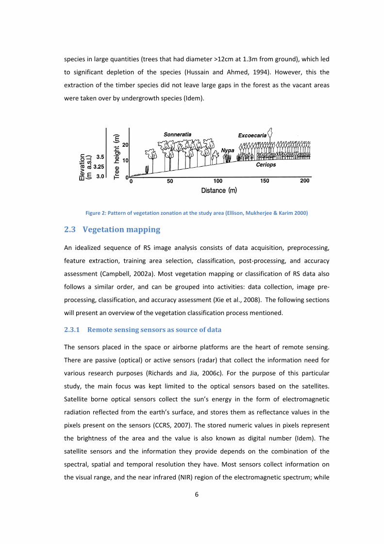
The flora of Sundarban is mostly characterized by the abundance of four species, Heritiera
fomes (Sundri), Excoecaria agallocha (Gewa), Ceripos decandra (Goran), and Sonneratia
apetala (Keora) (Karim, 1994); and the latter three are found in the study area. From the
published vegetation map published by the Forest Department of Bangladesh (Akhter et al.,
2002)it was observed that Goran and Gewa are the dominating vegetation species, and two
small patches of Keora exists in the north eastern part of the study area. Goran and Gewa
were found to form large areas of mixed vegetation in the study area. Goran and Gewa
were also found to form mono-specific zones. Karim (1994) classified Korea and Gewa as
trees, and Goran as shrub or small tree.
Karim (1994) suggested that Sundarban is dominated by evergreen trees that has mostly
heterogeneous structures and compositions. In some areas mono-specific vegetation stand
are found when very specific habitat requirements are met. Karim (1994) also divided the
Sundarbans into three salinity zones, and the western part of Sundarban including the
study area is in the 'Polyhaline Zone' or area of high salinity. This salinity zone is dominated
by Gewa and Goran species with height less than 11 meters. Karim (1994) also
characterized western Sundarban into mudflats and back-swamps. Mudflats occur next to
the water ways and are more diverse than the back-swamps, but in both case Goran is the
main species that forms the undergrowth. The mudflats may contain zones of single species
including Keora and Goran, whereas the back-swamps consists of mixed species areas
mostly with Gewa forming the canopy and Goran forming the understory. The back-swamp
ranges from well stratified vegetation to very sparse vegetation areas.
Ellison et al. (2000) also confirmed that zonation of mangrove vegetation in Sundarban is
found only for a small number of species including Goran and Keora. Gewa species exhibits
moderate zonation patterns and is only associated to gradients of salinity. It was also
suggested that the three dominant species has a gradient of occurrence closely dependant
on salinity.
To combat degradation of the forest resources the government of Bangladesh has place a
moratorium on timber extraction since 1989 (Hussain and Ahmed, 1994, Akhter, 2006).
Before 1989, the timber was extracted for various purpose including extraction of the Gewa
6
species in large quantities (trees that had diameter >12cm at 1.3m from ground), which led
to significant depletion of the species (Hussain and Ahmed, 1994). However, this the
extraction of the timber species did not leave large gaps in the forest as the vacant areas
were taken over by undergrowth species (Idem).
Figure 2: Pattern of vegetation zonation at the study area (Ellison, Mukherjee & Karim 2000)
2.3 Vegetation mapping
An idealized sequence of RS image analysis consists of data acquisition, preprocessing,
feature extraction, training area selection, classification, post-processing, and accuracy
assessment (Campbell, 2002a). Most vegetation mapping or classification of RS data also
follows a similar order, and can be grouped into activities: data collection, image pre-
processing, classification, and accuracy assessment (Xie et al., 2008). The following sections
will present an overview of the vegetation classification process mentioned.
2.3.1 Remote sensing sensors as source of data
The sensors placed in the space or airborne platforms are the heart of remote sensing.
There are passive (optical) or active sensors (radar) that collect the information need for
various research purposes (Richards and Jia, 2006c). For the purpose of this particular
study, the main focus was kept limited to the optical sensors based on the satellites.
Satellite borne optical sensors collect the sun’s energy in the form of electromagnetic
radiation reflected from the earth’s surface, and stores them as reflectance values in the
pixels present on the sensors (CCRS, 2007). The stored numeric values in pixels represent
the brightness of the area and the value is also known as digital number (Idem). The
satellite sensors and the information they provide depends on the combination of the
spectral, spatial and temporal resolution they have. Most sensors collect information on
the visual range, and the near infrared (NIR) region of the electromagnetic spectrum; while

7
others include these range and more, such as the middle infrared or thermal region. The
temporal resolution can vary from few minute to weeks depending on the orbit of the
satellite (Landgrebe, 2003, CCRS, 2007). Most satellites used for vegetation mapping are on
sun-synchronous orbit where the revisit time of the same place on the earth’s surface
ranges from 2-16 days (Xie et al., 2008).
Since different objects reflect sun’s energy uniquely or have unique spectral features, they
can be identified using remote sensing imagery. Vegetation in particular reflects less in the
visible range but the reflection increases dramatically in the NIR region. This feature is
largely utilized in vegetation mapping by differencing the radiances in the red and near-
infrared regions. The radiances in these regions are incorporated into the spectral
vegetation indices (VI) that are closely related to the fraction of radiation intercepted by
the photosynthetically active parts of trees (Campbell, 2002c).
Figure 3: Typical spectral signatures of photosynthetically active and non-photosynthetically active vegetation
(Beeri et al., 2007)
Selection of the appropriate RS sensors for vegetation mapping is very important as sensors
have different spatial, temporal, spectral and radiometric characteristics. The selection of
sensors is largely determined by four related factors: (i) the mapping objective
(scale/resolution, accuracy), (ii) the cost of images, (iii) the weather conditions (especially
atmospheric conditions) and (iv) the technical issues for image interpretation (pre-
processing, quality)(Xie et al., 2008).
Xie et al., (2008) provide a good summary of the satellites used for various vegetation
mapping worldwide over the years, and are presented in the following table.

8
Sensors Features Vegetation mapping applications
Landsat
TM
Medium to coarse spatial resolution with
multispectral data (120 m for thermal infrared band
and 30 m for multispectral bands) from Landsat 4 and
5 (1982 to present). Each scene covers an area of 185
x 185 km. Temporal resolution is 16 days.
Regional scale mapping, usually
capable of mapping vegetation at
community level.
Landsat
ETM+
Medium to coarse spatial resolution with
multispectral data (15 m for panchromatic band, 60m
for thermal infrared and 30m for multispectral
bands) (1999 to present). Each scene covers an area
of 185 km x 185 km. Temporal resolution is 16 days.
Regional scale mapping, usually
capable of mapping vegetation at
community level or some dominant
species can be possibly discriminated.
SPOT A full range of medium spatial resolutions from 20 m
down to 2.5 m, and SPOT VGT with coarse spatial
resolution of 1 km. Each scene covers 60 x 60 km for
HRV/HRVIR/HRG and 1000 x 1000 km (or 2000 3
2000 km) for VGT. SPOT 1, 2,3, 4 and 5 were
launched in the year of 1986, 1990, 1993, 1998 and
2002, respectively. SPOT 1 and 3 are not providing
data now.
Regional scale usually capable of
mapping vegetation at community
level or species level or
global/national/regional scale (from
VGT) mapping land cover types (i.e.
urban area, classes of vegetation,
water area, etc.).
MODIS Low spatial resolution (250–1000 m) and
multispectral data from the Terra Satellite (2000 to
present) and Aqua Satellite (2002 to present). Revisit
interval is around 1–2 days. Suitable for vegetation
mapping at a large scale. The swath is 2330 km (cross
track) by 10 km (along track at nadir).
Mapping at global, continental or
national scale. Suitable for mapping
land cover types (i.e. urban area,
classes of vegetation, water area, etc.).
AVHRR 1-km GSD with multispectral data from the NOAA
satellite series (1980 to present). The approximate
scene size is 2400 x 6400 km
Mapping at global, continental or
national scale. Suitable for mapping
land cover types (i.e. urban area,
classes of vegetation, water area, etc.).
IKONOS It collects high-resolution imagery at 1 m
(panchromatic) and 4 m (multispectral bands,
including red, green, blue and near infrared)
resolution. The revisit rate is 3–5 days (off-nadir).The
single scene is 11 x 11 km.
Local to regional scale vegetation
mapping at species or community level
or can be used to validate other
classification result.
QuickBird High resolution (2.4–0.6 m) and panchromatic and
multispectral imagery from a constellation of
spacecraft. Single scene area is 16.5 x 16.5 km. Revisit
frequency is around 1–3.5 days depending on
latitude.
Local to regional scale vegetation
mapping at species or community level
or can be used to validate other
classification result.
ASTER
Medium spatial resolution (15–90 m) image with 14
spectral bands from the Terra Satellite (2000 to
present). Visible to near-infrared bands have a spatial
resolution of 15 m, 30 m for short wave infrared
bands and 90 m for thermal infrared bands.
Regional to national scale vegetation
mapping at species or community level.
Hyperion
It collects hyper-spectral image with 220 bands
ranging from visible to short wave infrared. The
spatial resolution is 30 m. Data available since 2003.
At regional scale capable of mapping
vegetation at community level or
species level.
Table 1: Main features of image products from the different sensors (Xie et al., 2008).

9
2.3.2 Image preprocessing
This step is intended to make correction to the sensor-specific and platform-specific
radiometric and geometric distortions of data. Geometric correction refers to the
registration of the image to the ground by using proper coordinates to avoid the distortion
created the shape the earth’s surface (CCRS, 2007). The outcome of the geometric
correction is expected to be within +/- 1 pixel of the true location of the image, which is
achieved by using ground control points most notable in the image (Richards and Jia,
2006a).
Radiometric correction is the prerequisite for any change detection study carried out using
satellite images, since atmospheric condition, angle of the sun, seasonality etc. can have a
significant effect on the images (CCRS, 2007). There are many methods of radiometric
correction but all has the main objective of improving the fidelity of the brightness values
encoded in the satellite image or otherwise ‘restore’ the pixel with corrected value. Since
the exactly correction needed is difficult to know, analysts need to decide on how much
correction measures to be applied to an image(Campbell, 2002d).
2.3.3 Classification techniques
Common classification processes can be broadly grouped into two categories; i) un-
supervised classification and ii) supervised classification (CCRS, 2007, Campbell, 2002a)
Unsupervised methods are based on the values encoded in each pixel in the several
spectral bands of the satellite image, and require no prior knowledge on landscape for
classification (Campbell, 2002b). Unsupervised classifications uses clustering algorithm to
convert raw satellite images into multiple classes to provide useful information (Richards
and Jia, 2006b). ISODATA and K-means are probably the two most common unsupervised
clustering algorithms used for creating thematic maps from satellite imageries and are
found widely in image processing software packages(Xie et al., 2008).
Supervised classifications on the other hand can be defined as a process where pixels of
known classes or identity are used for classifying the pixels of unknown classes or identity
(Campbell, 2002b). The samples of the known identity are taken from training areas or
training fields (Idem). The underlying assumption of this process is that sufficient known
pixels for each class of interest are available so that representative signatures can be
developed for those classes (Richards and Jia, 2006b). The selection of appropriate training
10
areas depends on the analyst's familiarity with the study area and knowledge of the actual
surface cover types present in the image. Therefore, the analyst is said to be "supervising"
the categorization of a set of specific classes (CCRS, 2007). There are many supervised
classification methods available. Some examples may include, Parallepiped classification,
Minimun Distance classification, Maximum Likelyhood classification (MLC), Bayes’s
classification etc. (Campbell, 2002b), and MLC is probably the most commonly used
supervised classification technique (Xie et al., 2008). Apart from the supervised and
unsupervised classification techniques mentioned above there are many other methods
such as artificial neural network (ANN), decision tree (DT), fuzzy logic approaches,
supervised and unsupervised spectral angle classifiers, textural classification, non-
parametric classifier that are available today for use (Richards and Jia, 2006b, Campbell,
2002b).
ANN, DT, fuzzy logic approach methods each has their own advantages and disadvantages.
ANN is very useful as it can be applied to almost any form of data and can achieve 15%
greater accuracy than the MLC, but has been criticized for its black-box approach that
makes interpretation of the analytical process very difficult. Fuzzy logic approaches has
been found useful in mixed forest class areas, and DT has found to perform better that MLC
and ANN in multi-spectral imagery, but not in the case when hyper-spectral images were
used(Xie et al., 2008).
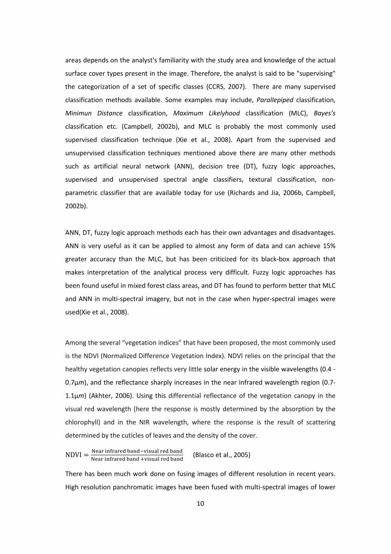
Among the several “vegetation indices” that have been proposed, the most commonly used
is the NDVI (Normalized Difference Vegetation Index). NDVI relies on the principal that the
healthy vegetation canopies reflects very little solar energy in the visible wavelengths (0.4 -
0.7μm), and the reflectance sharply increases in the near infrared wavelength region (0.7-
1.1μm) (Akhter, 2006). Using this differential reflectance of the vegetation canopy in the
visual red wavelength (here the response is mostly determined by the absorption by the
chlorophyll) and in the NIR wavelength, where the response is the result of scattering
determined by the cuticles of leaves and the density of the cover.
NDVI = ����� ������������������������� �������������������� (Blasco et al., 2005)
There has been much work done on fusing images of different resolution in recent years.
High resolution panchromatic images have been fused with multi-spectral images of lower

11
resolution, and it has been found to be a good technique for vegetation classification. There
are many others classifiers that exist today including approaches that combine multiple
methods to classify vegetation from a single satellite image. Researcher are still working on
creating better performing classification, as there are still no super-classification methods
that can be applied universally (Xie et al., 2008).
2.3.4 Accuracy assessment
Of the cartographic and classification accuracy assessment (Goodchild, 1994), vegetation
mapping is mostly concerned with the latter. The most widely used and accepted accuracy
assessment of thematic accuracy is the error matrix(Congalton and Green, 2009a). Error
matrix describes the fitness between the derived classes and the reference data using
overall class performance or kappa statistics. Individual class performance can also be
derived using confusion matrix if required (Idem).
2.4 Mangrove
Tomlinson (1995)defines mangrove as the tropical trees that are restricted to intertidal and
adjacent communities and also notes that the word “mangrove” has been frequently used
to refer to the community of the plants or the intertidal ecosystem. Mangrove forests cover
at least 14 million hectares in world (Kanniah et al., 2007) and acts as a very important
costal resource. Mangrove forests are important throughout the tropics as fishing areas,
nursery areas for the juveniles of many commercial fish and crustacean species, wildlife
reserves, plays important roles in coastal protection and water quality for recreation, used
as human habitation and aquaculture, and mangrove vegetation is harvested directly as
feed supplement and for timber products (Green et al., 1998).
2.4.1 Mangrove classification using remote sensing
The application of remote sensing methods to the study of mangroves roughly started
during 1970’s in larger mangrove forests especially in the Sundarban mangrove forest of
the Gangetic deltas. The first atlas of the mangroves was compiled in 1997, and the first
world wide inventory of the mangroves was carried out by the European Community in
2000 using remote sensing techniques (Blasco et al., 2005).
The location restriction of the mangroves near tropics, and the presence of water or wet
soil underneath the trees help mangroves to be identified easily, by using the remote

12
sensing. Since they are mostly present in the tropics, mangroves essentially have evergreen
canopies, thus use of NDVI is common to detect mangroves. Jensen et al., (1991) found that
NDVI is correlated to canopy closure (r=0.91) of mangroves, which can also be used to
measure mangrove density. Visual interpretation and temporal RS data series had also
been used interpreting features of mangroves. Apart from the classifiers, a combination
approach of blending images from optical and radar sensors were also applied to some of
the studies on mangrove. Particular use of Synthetic Aperture Radar (SAR) has shown good
potential in classifying mangroves according to height classes and based on homogeneity,
but at the same time, it should be mentioned that it is harder to obtain vegetation data
from the SAR images than the images obtained by optical sensors. Nevertheless, radar
sensors are a good option for areas that stay under cloud cover during most of the year
(Green et al., 1998).
Figure 4: Map of mangroves distribution around the world (Mangrove, 2009)
Aerial photographs have been used for many years to successfully classify mangroves with
high accuracy. Aerial photographs have also been successfully used by experts to separate
different species of trees within one stand (Blasco et al., 2005). The use of RS data provides
an advantageous solution to the task of studying mangrove areas effectively, and to
monitor changes over time accurately, rapidly, and cost-effectively. RS data has been used
to monitor deforestation and aquaculture activity around sensitive mangrove areas, in
environmental sensitivity analyses and for resource inventory and mapping purposes of the
mangroves. The results achieved in mangrove classification, however, are dependent on
the RS sensors that have been used for the particular study. It has also been said that the

13
result accuracy in the mangrove classification is also a function of the expert knowledge
and the ancillary data available at hand (Green et al., 1998). Green et al.,(1998) also
compared different methods of classifying mangroves, and found that LANDSAT TM was
the most efficient in separating non-mangroves from the mangroves.
Assessing the available literature Blasco et al. (2005) divided the mangrove classification
results into seven most useful physiognomic classes that have so far have been successfully
identified using RS data. A brief description of the classes follows:
Dense natural mangroves: is the most important class in a mangrove forest, and are often
located in protected areas. Dense mangroves consist of diverse species compositions, and
the ground coverage often exceeds 80%.
Degraded mangroves: is the forest area with a ground coverage of about 50–80% by trees
and shrubs. The spectral signal of this class integrates the response of chlorophyll elements
from the tree canopies and water-soaked soils beneath.
Fragmented mangroves: is the area where trees have ground coverage of about 25–50%.
The spectral signature of this class is primarily determined by the moist soils underneath
the trees, although the response of the green vegetation remains noticeable.
Leafless mangroves: as mangroves are usually evergreen trees, a strong absorption in the
NIR band (0.70–0.95 m) is thus considered abnormal, and indicates absences of tree foliage.
This kind of leaf shedding occurrence may be induced either by mass mortality of mangrove
trees (that occurred in Gambia, Côte d’Ivoire, etc.) or by unexplained diseases (virus,
insects, etc.).
Mangrove deforestation areas or clear felled mangroves: opening in mangrove forest
canopy caused by exploitation and clear felling can be detected from RS data easily. The
openings have corresponding pixels of water at high tide or by crusts of sodium chloride
deposits during the dry season at low tide.
Mangrove converted to other uses: The most conspicuous impacts on mangrove
ecosystems caused by anthropogenic activities is their conversion to shrimp ponds
(Thailand, Ecuador, Viet Nam, Indonesia, Bangladesh etc.) or to agriculture (mainly paddy
fields in Asia and West Africa). The mangroves converted to other uses can be easily
identified using time series data. The spectral signature of irrigated crops, mainly paddy
fields and sugarcanes, are very different from mangroves (strong absorption in the NIR

14
band). A lot of studies have been conducted to detect the mangroves conversion into other
uses using RS data.
Restored mangroves and afforestation areas: mangrove restoration sites or afforestation
activities often correspond to recently accreted intertidal zones or islands with dense
vegetation. Monitoring of such areas has been at the mouth of the Ganges (Bangladesh)
using RS, where the rate of survival and growth of Sonneratia apetala has been found to be
starkly different from one island to another. Dense vegetation with only one planted
species have a high photosynthetic activity that causes high absorption of photons and low
response in the wavelength 0.6–0.7 m, which make them easier to identify.
2.4.2 Mangrove classification using high spatial resolution satellite image
In recent years, researches have been undertaken to classify mangrove vegetation using
visual interpretation (Dahdouh-Guebas et al., 2004), pixel-based (Kanniah et al., 2007), and
object-based classification (Wang et al., 2004). Wang et al. (2004) also compared mangrove
classification results of pixel-based and object-based methods and proposed a hybrid
classification method based on their work in Panama.
Dahdouh-Guebas et al. (2004) were able to visually distinguish mangrove species from the
same genus using a pan-sharpened false colour composite IKONOS image of their study
area in Sri Lanka. Kanniah et al. (2007) conducted pixel-based classification of mangrove
species using an IKONOS image in Malaysia with 82% overall accuracy. Wang et al. (2004)
conducted their study of the mangroves in the Caribbean coast of Panama using IKONOS
image; and produced results of 89% accuracy using Maximum Likelihood classifier (pixel-
based), 80.4% accuracy using Nearest Neighbour (object-based method), and 91.4% overall
accuracy using a combined method. Everitt et al., (2009) followed methods developed by
Wang et al., and reproduced an average accuracy of 90% mapping Black Mangroves in
Texas.
2.4.3 Previous remote sensing studies in Sundarban
Like many other places, most of the inventories of Sundarban have been based on aerial
photos. The last official forest inventory was conducted in 1995 using aerial photos and a
digital database was created based on the inventory results. However, no updates were
made following the completion of the digital data base (Akhter 2006). The first forest
inventory result involving aerial photos was published in 1960 and the second one in 1985
15
(Chowdhury and Ahmed, 1994). Iftekhar and Islam (2002) had studied the change of
vegetation of SRF over time using forest inventory data, but their study did not involve in
new remote sensing data collection. Islam et al. (1997) studied the change of the
vegetation of Sundarban using aerial photographs, Landsat TM image of 1990 and other
ancillary data. Syed et al. (2001) conducted a research combining Landsat TM and Radar
data to detect the edge of the fragmented mangroves in the Sundarban. Akhter (2006)
attempted to create a monitoring model of vegetation change in Sundarban using RS data
(Landsat ETM+ of 2000 and Landsat TM of 1989) to classify the vegetation. Her study
involved only north-eastern part of the Sundarban forest, and the study achieved an overall
accuracy of 78% when eight classes were used during classification using Landsat TM image
with MLC. Emch and Peterson (2006) conducted another study using the same data as
Akhter (2006) to produce forest cover maps for further change detection study. They
selected training data from the 1985 inventory derived map and MLC to classify the Landsat
images. Their study area encompassed most of the Sundarban forest area of Bangladesh. In
addition to the MLC, they also used NDVI transformation of the images in a sub-pixel
assessment to assess density change of the forested area. Another unpublished MSc.
dissertation (Alam, 2008)was found to used the same data as Emch and Peterson, and
Akhter, to classify the vegetation species of the same study area as of Akhter. Giri et al.,
(2007) used Landsat and QuickBird scenes with a focus on monitoring the overall mangrove
deforestation change over time, but not to classify the vegetation.
However, during the literature review, no research work has been found describing the use
of very high resolution optical RS images (such as IKONOS or QuickBird) or object-based
algorithms to classify vegetation in the SRF.

16
3. Data and Methods
3.1 Data
Several QuickBird scenes of the Sundarban area are available in the public domain and can
be obtained from the website of the Global Landcover Facility (GLF). One of such image
covering the study area was used for vegetation classification. A subset of Landsat TM
image covering the study area was also used for the classification purpose. Landsat images
are available from the U.S. Geological Survey (USGS) free of cost. Digital forest map in
vector format prepared in 1997 by Bangladesh Forest Department from previous forest
inventory data using 1:15000 scale aerial photographs (Akhter 2006) was used as a ground-
truthing source. Further details of these three data types are provided in the following
sections.
3.1.1 Landsat TM
The Landsat TM scene was obtained from the internet using the 'Glovis' tool of USGS
(USGS, 2002). The Landsat TM scene was captured on the 04 Nov 2004, and the path of the
satellite was 134 and the start and end row was 45. Landsat TM has seven bands with 30m
pixel size or spatial resolution (band 6 has 120m pixel size) with 8-Bit radiometric
resolution; 16 days revisit time; and single images that cover an area of 170x185 km2 each
(USGS, 2009). The range that each band covers in electromagnetic spectrum is given in the
following:
o Band 1 Visible (0.45 – 0.52 µm)
o Band 2 Visible (0.52 – 0.60 µm)
o Band 3 Visible (0.63 – 0.69 µm)
o Band 4 Near-Infrared (0.76 – 0.90 µm)
o Band 5 Near-Infrared (1.55 – 1.75 µm)
o Band 6 Thermal (10.40 – 12.50 µm)
o Band 7 Mid-Infrared (2.08 – 2.35 µm) (USGS, 2004)
The downloaded image comes with a standard terrain correction (Level 1T) that provides
systematic radiometric and geometric correction using ground control points from the
Global land Survey 2005 (USGS, 1999). The Landsat TM image have a 50m positional RMS
error (USGS, 1999). The metadata that came with the image file suggests that the image

17
was in GeoTIFF format, in Universal Transverse Mercator (UTM) projection system and falls
in zone 45 north. During the acquisition the sun azimuth was 146.4 and the sun elevation
was 46.38, and the scene had 2% cloud cover present.
3.1.2 QuickBird
The QuickBird image was downloaded free of charge from the Global Land Cover Facility
website (DigitalGlobe, 2004). A QuickBird image provides a resolution of 61 cm in
panchromatic band and 2.4m in four channel multi-spectral band at nadir with 11-Bit
radiometric resolution. Revisit period of QuickBird satellite is three to seven days and a
single image covers an area of 16.5km x 16.5 km or in stripes up to 115km x 16.5 km.
QuickBird scene in multispectral image covers the following area in electromagnetic
spectrum:
o Band 1 Blue (0.45 – 0.52 µm)
o Band 2 Green (0.52 – 0.60 µm)
o Band 3 Red (0.63 – 0.69 µm)
o Band 4 Near-Infrared (0.76 – 0.90 µm),
and the panchromatic band cover a range of 0.445 - 0.9 µm. Standard QuickBird image
provides positional accuracy within 23 meters even without Geometric correction using
ground control points (DigitalGlobe, 2010). Metadata accompanying the QuickBird scene
suggests that the image is acquired on 02 Dec 2004, and projected to UTM in 45 north
zone. Sun azimuth during acquisition was 156.4 and sun elevation was 42.4, and the image
was acquired with an off-nadir angle of 5.9. Due to the fact that the image was captured
off-nadir the pixel size of the multispectral bands was 2.8m and the panchromatic band has
a pixel size of 0.70m. Consulting the QuickBird product guide it was revealed that the
downloaded product was their standard product which suggests that it was terrain
corrected using a coarse DEM, radiometric and sensor correction has also been applied to
the product. The QuickBird product came in a zipped format that contained the metadata,
multispectral (MS) image, and panchromatic image separately.
3.1.3 Vector Map
A digital vegetation map of the SRF in vector form (Shape file) will be used for the ground
verification purpose. The vector map was created by Forest Department (FD) of Bangladesh

18
under the FRMP project during 1996-98. The source data was pan-chromatic aerial
photographs of 1:15000 scale taken in 1995. A forest vegetation map was created using
stereoscopic interpretation of the aerial photographs and ground based field surveys of the
same year. This map was then digitized to create the digital database of vegetation
inventory of SRF and to create the digital vector map in shape file format of the vegetation
species (Akhter, 2006).
Inspection of the vegetation shape file revealed 22 attributes, of which five is relevant to
the present study, namely 'Vegetation Type', 'Mixture', 'Area', 'Height', and 'Closure'. There
are three species of flora found for the study are, which are 'Goran' or Ceriops decandra,
'Gewa' or Excoecaria agallocha, and 'Keora' or Sonneratia apetala, that makes up all the
vegetation type combinations. The vegetation types found are, Goran, Goran-Gewa, Gewa,
Gewa mathal (coppice), Gewa-Goran, Keora, grass and bare ground. The classification
method was adopted from the earlier inventory made during 1985 (Akhter, 2006).
Following table summarizes the relevant classification rule utilized by Chaffey, Miller &
Sandom (1985).
Vegetation types
Composition by species (%)
Goran Gewa Keora
Goran >=75
Goran-Gewa 50-75 25-50
Gewa >=75
Gewa-Goran 25-50 50-75
Keora
>=90
Table 2: Conditions used to create the vegetation classes
The shape file also contain record of scattered species located within the polygons of the
above mentioned vegetation types, under the attribute name 'Mixture'. The scattered
species found within the study areas are: Baen (Avicennia alba/marina/officinalis) , Dhundal
(Xylocarpus granatum), Passur (Xylocarpus mekongensis) , and Keora (Sonneratia apetala).
The scattered species are found in combination of Baen and Dhundal, Passur or Dhundal, or
as a single species in case of Keora. However, 92% of the study area does not contain any
scattered species.

19
The 'Height' attribute divides the polygons in five classes. For water body the class is not
available or 'NA', and then there are height classes less than five meters (<5m), in between
five to ten meters (<10m=>5m), in between ten to fifteen meters (<15m=>10m), and lastly
greater than fifteen meters (=>15m).
The 'Closure' attributes divides the areas depending on the vegetation canopy cover
present in each polygon. The closure classes are 'a' (=>70%), 'b' (<70%=>30%), 'c'
(<30%=>10%), and 'n.a.' or not available.
3.2 Software used for the study
Four software were used mostly during the research. Arcgis 9.3.1 was used for all kinds of
GIS analysis, ENVI 4.7 was used for remote sensing analysis (ENVI Zoom for imgae
segmentation and classification of objects), Microsoft Office 2007 suite was used for
drafting the dissertation and for spreadsheet necessities, and Google Earth has been used
for carrying out visual inspection of the study area in absence of any field visit.
3.3 Methods
As described in the research objective (section 1.1, p 1) the aim of this research is to
compare different data and classification methods to suggest the most effective
combination. The following workflow (figure 3) was adopted to carry out the analysis of the
satellite data.
Figure 5: Process path of the methodology
Images were first pre-processed, inspected for anomalies, training and testing samples
were created during the classification phase including classifying the images. After the
classification, the results were verified using confusion matrix in accuracy assessment steps.
Verified results of different methods were then compared to identify the most appropriate
method for the study area. Further descriptions of the methods used are detailed in the
following sections.
20
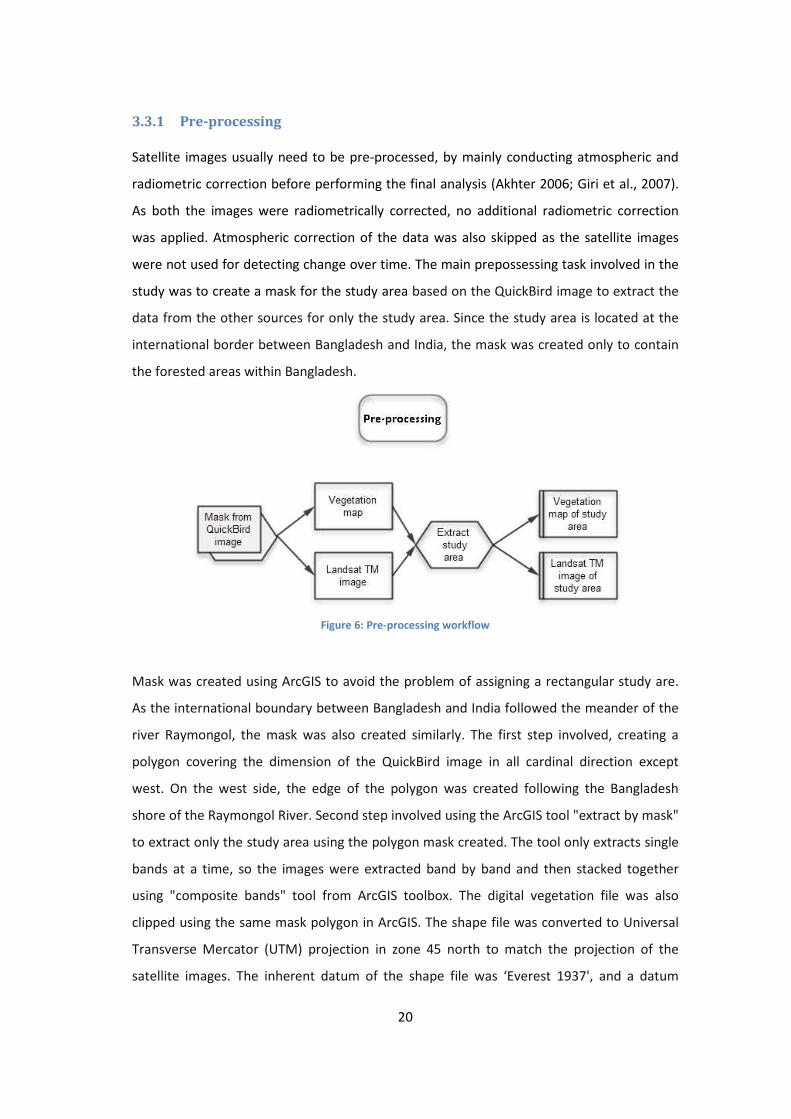
3.3.1 Pre-processing
Satellite images usually need to be pre-processed, by mainly conducting atmospheric and
radiometric correction before performing the final analysis (Akhter 2006; Giri et al., 2007).
As both the images were radiometrically corrected, no additional radiometric correction
was applied. Atmospheric correction of the data was also skipped as the satellite images
were not used for detecting change over time. The main prepossessing task involved in the
study was to create a mask for the study area based on the QuickBird image to extract the
data from the other sources for only the study area. Since the study area is located at the
international border between Bangladesh and India, the mask was created only to contain
the forested areas within Bangladesh.
Figure 6: Pre-processing workflow
Mask was created using ArcGIS to avoid the problem of assigning a rectangular study are.
As the international boundary between Bangladesh and India followed the meander of the
river Raymongol, the mask was also created similarly. The first step involved, creating a
polygon covering the dimension of the QuickBird image in all cardinal direction except
west. On the west side, the edge of the polygon was created following the Bangladesh
shore of the Raymongol River. Second step involved using the ArcGIS tool "extract by mask"
to extract only the study area using the polygon mask created. The tool only extracts single
bands at a time, so the images were extracted band by band and then stacked together
using "composite bands" tool from ArcGIS toolbox. The digital vegetation file was also
clipped using the same mask polygon in ArcGIS. The shape file was converted to Universal
Transverse Mercator (UTM) projection in zone 45 north to match the projection of the
satellite images. The inherent datum of the shape file was ‘Everest 1937', and a datum
21
projection was required to convert it to the datum WGS84. The inherent 'Everest 1937' has
the same properties as the 'Kalianpur_1937' inbuilt in ArcGIS program, therefore the
following parameters were used for datum transformation (Δx=282, Δy=726, Δz=254) as
suggested in the geographic transformation documentation provided with the ArcGIS
program. Nine ground control points were created using the QuickBird image the
vegetation was spatially adjusted to match the image using 'rubbersheet ' transformation.
The Landsat TM image was also geo-registered with the QuickBird image so that all data
had the same geo-reference.
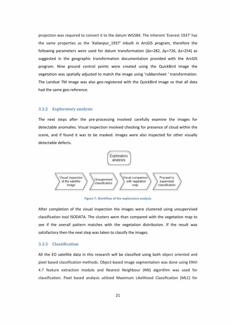
3.3.2 Exploratory analysis
The next steps after the pre-processing involved carefully examine the images for
detectable anomalies. Visual inspection involved checking for presence of cloud within the
scene, and if found it was to be masked. Images were also inspected for other visually
detectable defects.
Figure 7: Workflow of the exploratory analysis
After completion of the visual inspection the images were clustered using unsupervised
classification tool ISODATA. The clusters were than compared with the vegetation map to
see if the overall pattern matches with the vegetation distribution. If the result was
satisfactory then the next step was taken to classify the images.
3.3.3 Classification
All the EO satellite data in this research will be classified using both object oriented and
pixel based classification methods. Object-based image segmentation was done using ENVI
4.7 feature extraction module and Nearest Neighbour (NN) algorithm was used for
classification. Pixel based analysis utilized Maximum Likelihood Classification (MLC) for
22
supervised classification following the success of earlier studies (Akhter, 2006; Green et al.,
1998).
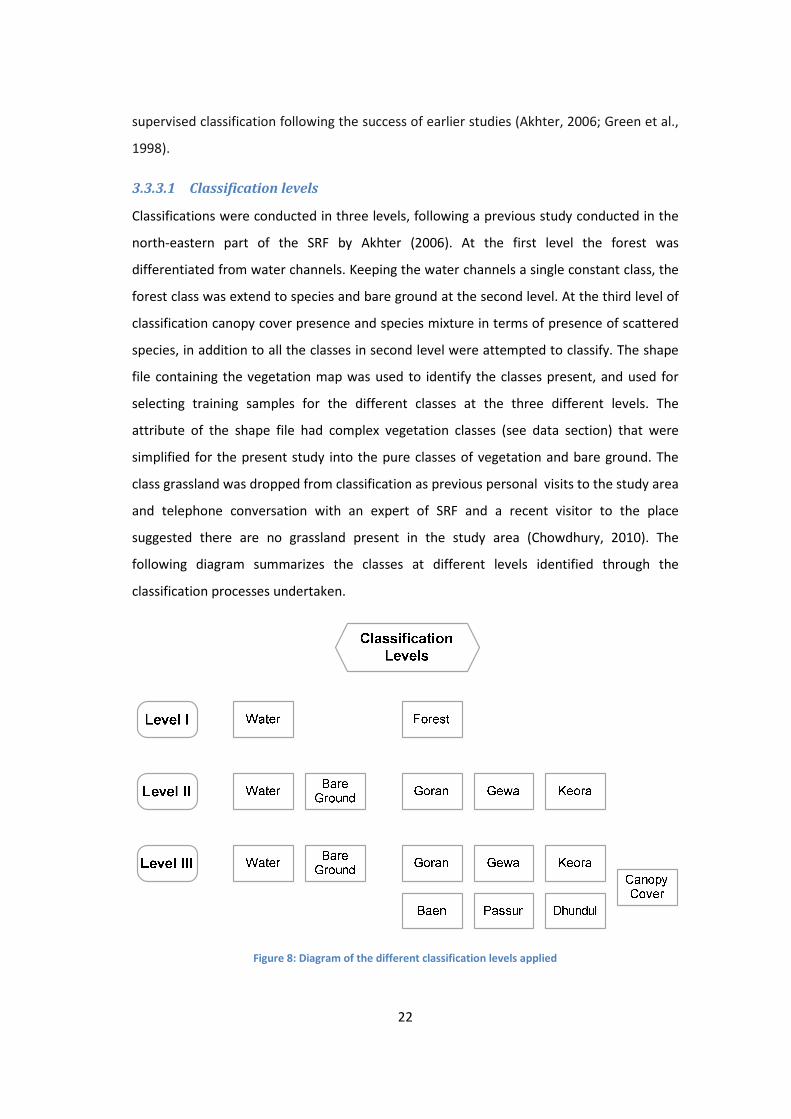
3.3.3.1 Classification levels
Classifications were conducted in three levels, following a previous study conducted in the
north-eastern part of the SRF by Akhter (2006). At the first level the forest was
differentiated from water channels. Keeping the water channels a single constant class, the
forest class was extend to species and bare ground at the second level. At the third level of
classification canopy cover presence and species mixture in terms of presence of scattered
species, in addition to all the classes in second level were attempted to classify. The shape
file containing the vegetation map was used to identify the classes present, and used for
selecting training samples for the different classes at the three different levels. The
attribute of the shape file had complex vegetation classes (see data section) that were
simplified for the present study into the pure classes of vegetation and bare ground. The
class grassland was dropped from classification as previous personal visits to the study area
and telephone conversation with an expert of SRF and a recent visitor to the place
suggested there are no grassland present in the study area (Chowdhury, 2010). The
following diagram summarizes the classes at different levels identified through the
classification processes undertaken.
Figure 8: Diagram of the different classification levels applied
23
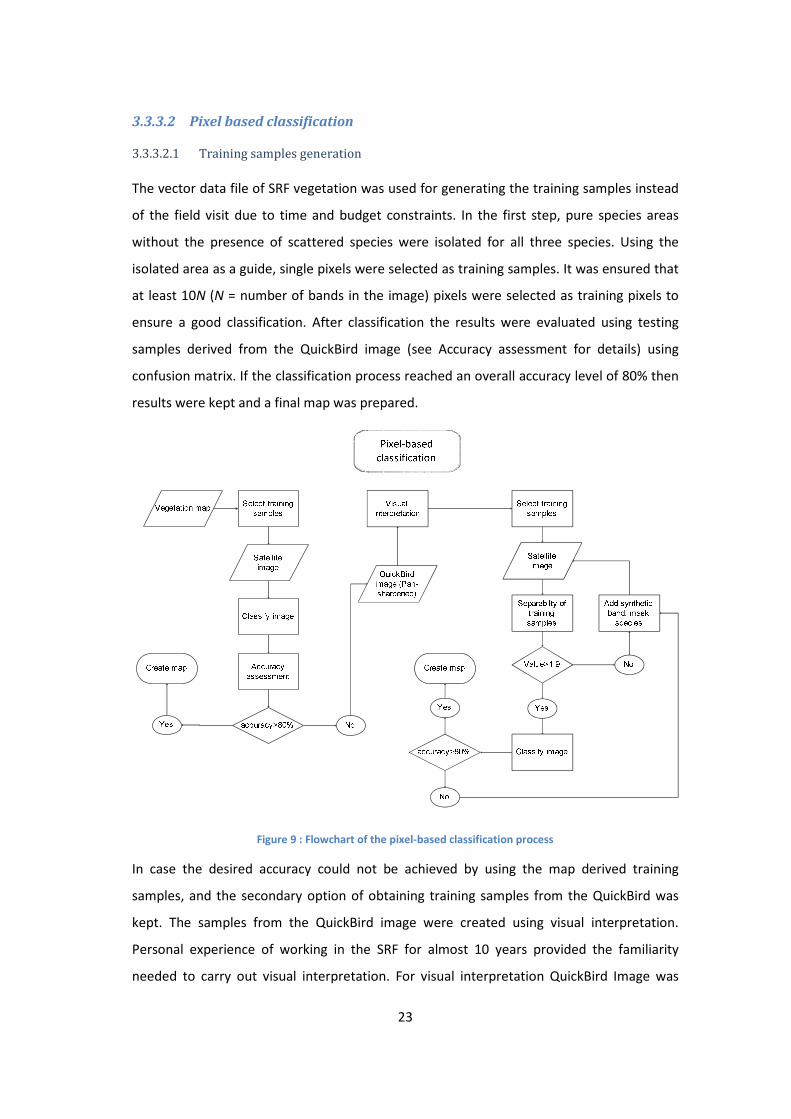
3.3.3.2 Pixel based classification
3.3.3.2.1 Training samples generation
The vector data file of SRF vegetation was used for generating the training samples instead
of the field visit due to time and budget constraints. In the first step, pure species areas
without the presence of scattered species were isolated for all three species. Using the
isolated area as a guide, single pixels were selected as training samples. It was ensured that
at least 10N (N = number of bands in the image) pixels were selected as training pixels to
ensure a good classification. After classification the results were evaluated using testing
samples derived from the QuickBird image (see Accuracy assessment for details) using
confusion matrix. If the classification process reached an overall accuracy level of 80% then
results were kept and a final map was prepared.
Figure 9 : Flowchart of the pixel-based classification process
In case the desired accuracy could not be achieved by using the map derived training
samples, and the secondary option of obtaining training samples from the QuickBird was
kept. The samples from the QuickBird image were created using visual interpretation.
Personal experience of working in the SRF for almost 10 years provided the familiarity
needed to carry out visual interpretation. For visual interpretation QuickBird Image was
24
pan-sharpened using ENVI 4.7's image sharpening tool. The HSV conversion method was
implemented as it provided best results for interpretation judged visually through trial and
error. The vegetation shape file was used as ancillary data for the visual interpretation.
To ensure the consistency of the vegetation interpretation, the species Gewa was identified
in two other QuickBird scenes (available at GLCF) ; one was from the eastern part of the SRF
and another from the western part of the SRF. At each time the attempt was made to pick
30 samples of Gewa from each QuickBird image within five minutes. The samples where
then used to create signature profiles using mean DN value and compared to the signature
generated from the study site to see whether interpretation was consistent.
The selected samples were then tested for their spectral separability using the Jeffries-
Matusita (J-M) index. The index values ranges from 0 to 2, where values between 0 to 1
represents very poor separability, values from 1 to 1.9 represents poor separability, values
above 1.9 to 2 represents good separability. The samples were tested pair-wise for their
separability in J-M index and were kept if values were above 1.9 (Angerer and Marcolongo,
2005, Richards and Jia, 2006a).
After the completion of collecting training samples the image was classified and the result
was assessed for accuracy. If results were satisfactory then the results were kept and the
final map was produced. However, unsatisfactory result meant continuation of
classification, creating more training samples, or masking vegetation that was spectrally
difficult to separate.
3.3.3.2.2 Significance of the middle infrared bands
Since the classification results were compared between Landsat TM and QuickBird
products, the significance of the middle infrared bands (band 5 and band 7) of Landsat TM
product needed to be measured. The QuickBird product does not include these two bands,
and therefore the impact that these two bands make were measured. To measure the
significance, classification of the Landsat TM image was conducted using only the bands
similar to QuickBird (Band 1-4 and NDVI). The results of classification using all bands and
NDVI of Landsat TM versus only Band 1—4 and NDVI were then evaluated and compared.
25
3.3.3.2.3 NDVI
Akhter (2006) found that inclusion of NDVI as a synthetic band with the existing bands
improves mangrove classification in Sundarban. Therefore, NDVI image was computed and
added to the both Landsat TM and QuickBird image for classification. The NDVI band was
converted from floating data to 8 bit for Landsat TM, and 11 bit for Quickbird image to
match their radiometric resolution.
NDVI values were also used to calculate the percentage cover of the canopy as Jensen et
al., (1991) found that the NDVI values are strongly related to the amount of canopy closure
(r=0.91).
3.3.3.3 Object-based classification
Object-based classification was performed using ENVI Zoom software. The software
performs image segmentation based on spatial, spectral, and texture characteristics of
multi-spectral or panchromatic image. The ENVI Zoom uses an edge-based segmentation
algorithm that only requires one input parameter 'Scale Level' (value ranges 0 to 100). The
segmentation algorithm yields multi-scale segmentation results from finer to coarser
segmentation, by suppressing weak edges to different levels (ENVI, 2008). The ENVI user
manual (2008) also mentions that choosing a high 'Scale Level' causes fewer segments to be
defined, and choosing a low 'Scale Level' causes more segments to be defined. The manual
suggests choosing the highest 'Scale Level' that delineates the boundaries of features as
well as possible. To identify the highest scale that delineates between the class at
classification level II, and objective approach was followed that was introduced by Wang et
al. (2004). The image was segmented from the starting 'Scale Level’ value of 5. The
segmented image was then intersected with the training samples used during the pixel-
based classification. The intersection selected the objects where the pixels samples fell, and
then the objects were separated and treated as training samples. Using the objects as
samples, pair-wise separability was computed using the J-M index. If the value was higher
than 1.9, then the samples were kept, and they were used for supervised classification
using the Nearest Neighbor (NN) algorithm inbuilt in ENVI. In case the separability was less
than 1.9, the 'Scale Level' was increased at an interval of 5, and continued till the process
yielded usable training sample for the object-based classification. If the process failed to
select appropriate training samples, then a hybrid object-based classification was carried.

26
At classification level I the highest scale was selected visually by observing result at the
preview window of the feature extraction process at ENVI, instead of exporting the results
at each scale level. It was assumed that with false color composite image it will possible to
visually separate water from forest areas.
To find possible influence of the scale level on classification of the vegetation, the average
size of objects was also calculated along with the highest scale level test. A 1 km2 area was
selected to reduce computational demand, avoiding large water channels. All objects at
each scale level that had their centroids within that square were selected for calculating the
mean area size per object. The maximum and minimum size of object at each scale level
was also calculated. Only QuickBird image was used for this study.
3.3.3.3.1 Hybrid object-based classification
In addition to the method introduced earlier to select the appropriate 'Scale Level' Wang,
Sousa and Gong (2004) also adopted a integrated classification method of using both pixel-
based and object-based classification by combining MLC and NN algorithms. They used the
object-based method to separate vegetation where accuracy was low using MLC. However,
for this study, a hybrid method of classification was developed by using the extracted
object from the segmented image, and combining the results from pixel-based method with
the objects, instead of using the methods separately. The procedure of the method is
detailed in the following section.
In first step the image was segmented and the results were exported as vector objects
using the ENVI feature extraction workflow. The segmentation process involves setting
appropriate 'Scale Level', and then merging the segments to form larger objects to reduce
over segmentation issue. The merge option in ENVI is developed based on the Lambda-
Schedule algorithm created by Robinson, Redding and Crisp (2002). The algorithm
iteratively merges adjacent segments based on a combination of spectral and spatial
information. Merging proceeds if the algorithm finds a pair of adjacent regions, i and j, such
that the merging cost ti,j is less than a defined threshold lambda value:
27
��,� =
|O�| ∗ �O��|O�| + �O��
∗ !� − !� #
lenght *∂,O�, O�-.
Where:
O� is region i of the image
|O�| is the area of region i
!� is the average value in region i
!� is the average value in region j
!� − !� is the Euclidean distance between the spectral values of regions i and j
lenght *∂,O�, O�-. is the length of the common boundary of O� and O�.
The scale level was set at the optimum from the results described in the earlier section.
Merge level was set at optimum visually as the ENVI feature extraction module provides an
interactive preview.
In the second step, the exported objects were used with the Hawth's tool to produce
'thematic raster summary' from the previously classified image using MLC. The outcome
had each object containing counts of each raster theme from the classified image stored in
a DBF file format. The dbf file was opened in Microsoft Excel 2007, and a majority class and
a class column was added to the DBF file. At the majority column using the 'Index' and
nested ‘MAX’ formula of MS Excel, the class having the majority pixel count was identified.
The other class column contained the thematic class derived by using nested 'if ' formula
with the same conditions used for creating the vegetation classes in the vegetation
database created by FD (see Table 2). Three more conditions: class = water>90, and class =
bare ground>75, class=mixed (if none of the conditions were met) were added to the rule.
Then the dbf file was joined with the shape file containing the exported objects, and final
maps were created using the majority and classes based on rules.
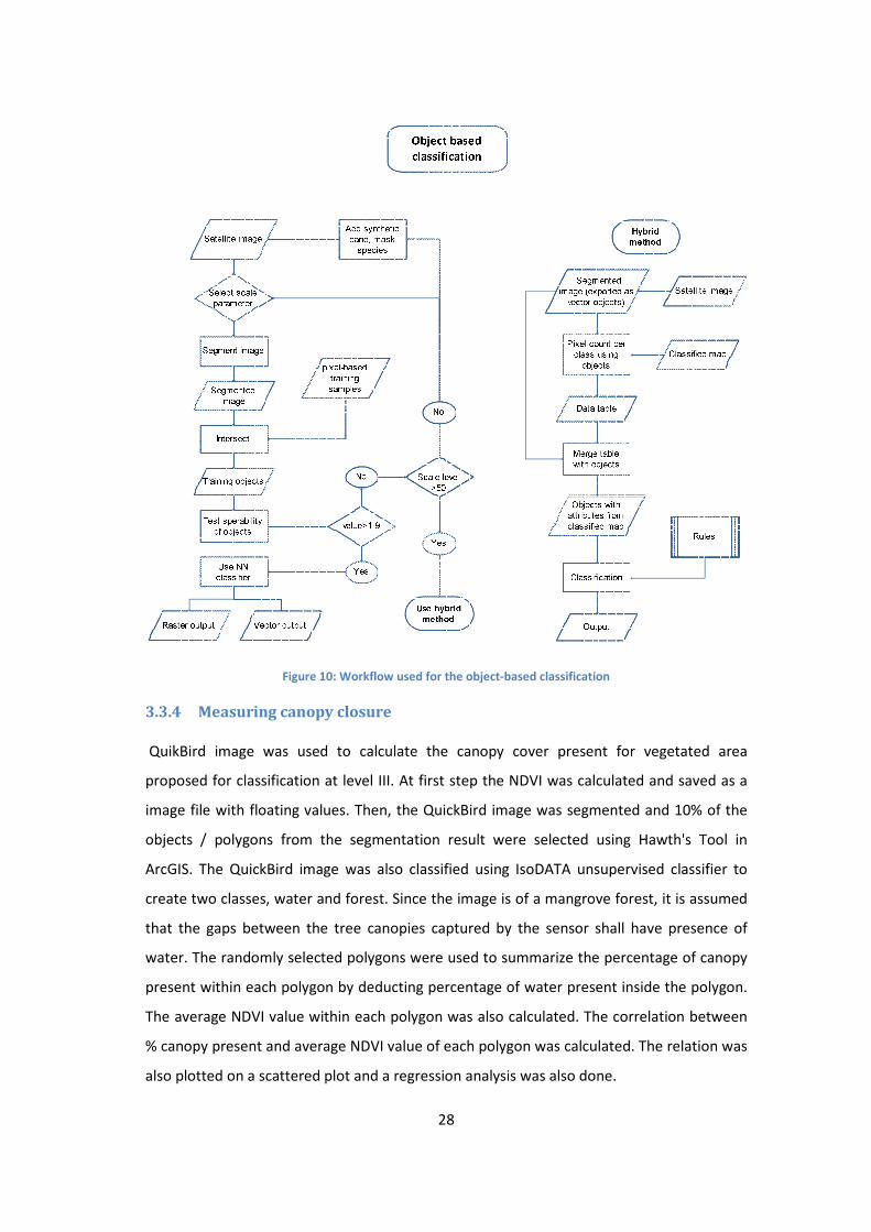
28
Figure 10: Workflow used for the object-based classification
3.3.4 Measuring canopy closure
QuikBird image was used to calculate the canopy cover present for vegetated area
proposed for classification at level III. At first step the NDVI was calculated and saved as a
image file with floating values. Then, the QuickBird image was segmented and 10% of the
objects / polygons from the segmentation result were selected using Hawth's Tool in
ArcGIS. The QuickBird image was also classified using IsoDATA unsupervised classifier to
create two classes, water and forest. Since the image is of a mangrove forest, it is assumed
that the gaps between the tree canopies captured by the sensor shall have presence of
water. The randomly selected polygons were used to summarize the percentage of canopy
present within each polygon by deducting percentage of water present inside the polygon.
The average NDVI value within each polygon was also calculated. The correlation between
% canopy present and average NDVI value of each polygon was calculated. The relation was
also plotted on a scattered plot and a regression analysis was also done.

29
A separate visual analysis was also conducted to evaluate the relation between NDVI values
and the canopy cover in the study area. Three canopy class, 'Low', 'Medium', and 'High' was
visually identified and 30 samples were selected from the 10% randomly selected polygons
described earlier. As a guiding rule, low canopy were selected if a polygon contained less
than 30% tree cover, medium canopy was considered if the polygon had more than 30%
canopy but less than 80%, and high canopy was considered to have more than 80% cover in
a polygon.
3.3.5 Accuracy assessment
Results of the classification was assessed using error matrix, as it is a very effective way to
assess accuracy of classification results of remotely sensed data(Congalton and Green,
2009a). Two different kinds of test samples were used, random test samples and stratified
random test samples.
200 random samples were created using ArcGIS and their class were visually interpreted
from QuickBird image. For level I classification, they were labeled only to water and forest,
and for level II and III it was labeled according to the classes used.
To generate the stratified random samples 1000 points were randomly generated. 50
points for each class were selected from the The QuickBird image according to the
classification level to meet the minimum requirement(Congalton and Green, 2009b) . If
sufficient number of samples was not possible to ensure for a class from the 1000 random
points, 1000 new points were created to collect rest required. To avoid having samples in
close proximity, polygons created from segmenting the QuickBird image (scale level 25 and
merge level 98 used with ENVI to produce segments) were overlaid on the image, and only
one sample per polygon was allowed.
The randomly collected and the stratified randomly collected test samples were used for a
pixel to pixel accuracy assessment. However, Russell & Green (2009b) suggest to use 3x3
pixel cluster for validating products derived from Landsat images, and 5x5 pixel cluster for
products made from VHR satellite image, such as QuickBird, to compensate for the
positional inaccuracy. Since the Landsat image was registered based on the QuickBird
image, and they have very different pixel size, it may have introduced unintentional
positional inaccuracy. Moreover labeling the randomly generated image was carried out
rigidly without consideration of the surroundings. It was expected that randomly generated

30
points may fall on boundary of two thematic classes, and only one class was to be assigned
in those clases. Therefore, the random 200 points were also used for creating 3x3 and 5x5
grids to assess the classification results of Landsat TM and QuickBird image respectively.
Apart from the location, it was expected that the random samples may not have sufficient
amount of test samples per thematic class; therefore stratified random test samples were
also collected.
Since the ground verification is carried out using visual interpretation by the analyst
without having an option for further validation, or having test samples from field visit, all
three types of test samples (see p29) were used in the study to assess accuracy. Using
three types of test samples would provide a range of the accuracy estimate for each
classification result, instead of a single value; therefore will provide a better picture for the
reader. However, it is was thought that the accuracy assessment results from the random
cluster and stratified random would provide a better result than the random pixel to pixel
assessment due to strict way labels were to assign to the random 200 points.
The three test sample selection process is summarized in the following Figure 11.
Figure 11: Accuracy assessment flowchart
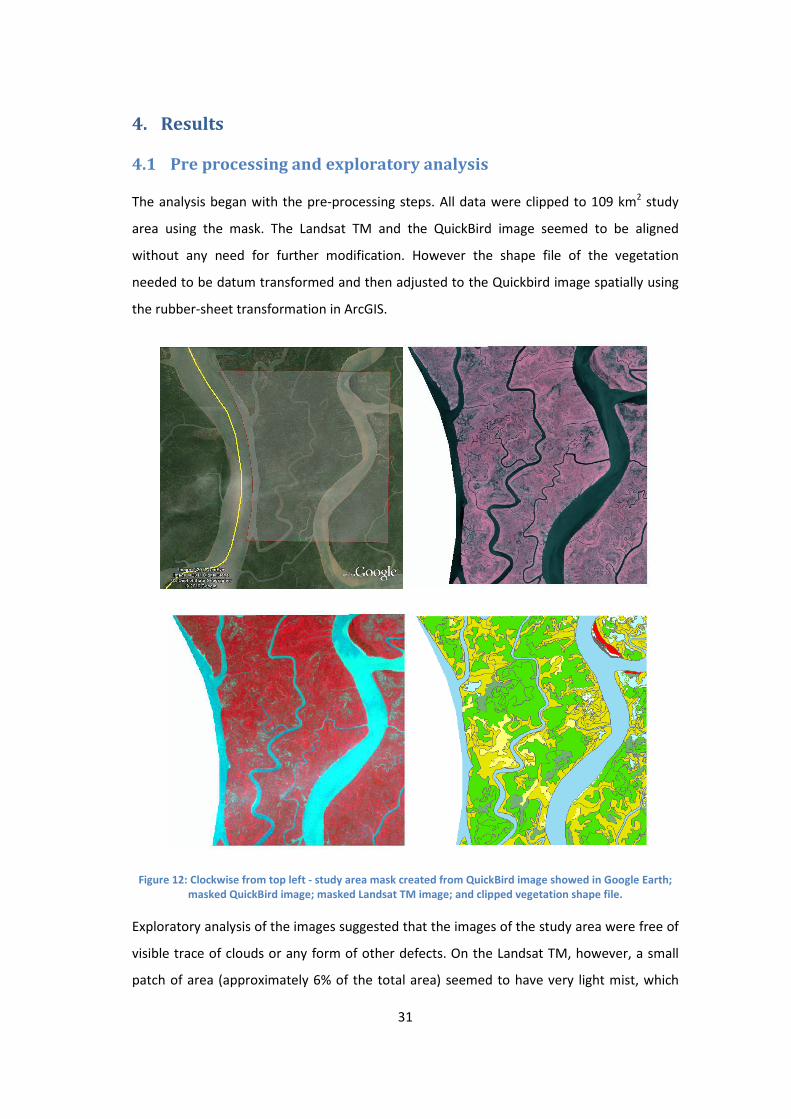
31
4. Results
4.1 Pre processing and exploratory analysis
The analysis began with the pre-processing steps. All data were clipped to 109 km2 study
area using the mask. The Landsat TM and the QuickBird image seemed to be aligned
without any need for further modification. However the shape file of the vegetation
needed to be datum transformed and then adjusted to the Quickbird image spatially using
the rubber-sheet transformation in ArcGIS.
Figure 12: Clockwise from top left - study area mask created from QuickBird image showed in Google Earth;
masked QuickBird image; masked Landsat TM image; and clipped vegetation shape file.
Exploratory analysis of the images suggested that the images of the study area were free of
visible trace of clouds or any form of other defects. On the Landsat TM, however, a small
patch of area (approximately 6% of the total area) seemed to have very light mist, which

32
was almost non-distinguishable. No additional treatment was applied as unsupervised
clustering results suggested that the presence of mist had no major impact on clustering
results. Visual inspection suggested that the QuickBird image was most likely acquired
during high tide, as there was visible presence of water inside most of the forested area
with low canopy cover. Due to presence of water inside the forest area, it was expected
that there would be confusion between bare ground and water classes during classification.
Landast TM image on the other hand was thought to be acquired during low tide due to the
presence of bare ground in areas not seen on QuickBird image. Large patches of vegetation
zones were easily identified on both Landsat TM and QuickBird image visually. Visual
inspection also indicated that the study area might be mostly dominated by Goran species,
and small patches of Gewa and Keora also exist. There were a lot of scattered trees seen
inside Goran dominated areas on QuickBird, and areas were classified as mixed areas on
the existing vegetation map. However, it was felt that the dominance of Goran was more
prominent than the vegetation map suggested.
The unsupervised classification was carried out with ISODATA algorithm to produce a total
of 35 classes. The Landsat TM results from unsupervised clustering showed close
resemblance to the species formation then that of the vegetation shape file. However, this
was only evident when Landsat TM was used without NDVI as an additional band. The
inclusion of NDVI caused a "salt and pepper" effect to the results.
The higher spatial resolution of the QuickBird image also resulted in a "salt and pepper"
outcome when put through the ISODATA clustering. The visual identification of the
QuickBird image was on the other hand easier for recognizing the existing vegetation
patterns and compare with the existing vegetation shape file.
During the exploratory analysis it was found that the vegetation map of FD was generalized
and in some areas the classes and attributes assigned to them did not match well with the
pan-sharpened image visual interpretation. In some places, when pure Gewa areas on the
vegetation map were overlaid on the QuickBird image, it was found that there were other
vegetation species besides Gewa. Some areas on the vegetation map labeled as Gewa were
seen to have a lot of bare ground, which could have been separated from the vegetated
areas.
33
4.2 Pixel-based classification
4.2.1 Level I classification
The level I classification was carried out with the training samples collected from the
vegetation shape file. The following table summarizes the accuracy results for both Landsat
TM and QuickBird image at level I classification using MLC classifier. All accuracy results
were above 90%. It was found that only the class 'water' was misclassified at level I. The
accuracy achieved was marginally higher when QuickBird image was used than that of
Landsat TM image.
Assessment using random testing samples provided lowest accuracy when used in pixel to
pixel evaluation for both the images; and when random test samples were used in clusters,
it produced the highest accuracy. Visual inspection aided by the pan-sharpened QuickBird
image suggested that test samples very close to the forest edge, and samples in very
narrow creeks caused misclassification of water into forest, for both image types.
Landsat TM QuickBird
Random Random
3x3 cluster Stratified Random
Random
Random
5x5 cluster Stratified Random
93.5 96.5 95.33 97.5 99.5 98.5
Table 3: Overall accuracy results at level I pixel-based classification. The values provided are in percentage.
4.2.2 Level II classification
The accuracy of classification result at level II was lower than the result of level I, and more
importantly varied much more across the different evaluation methods applied. It is also
important to note that the training samples created from vegetation shape file failed to
provide desired result in terms of accuracy. As a result new samples were obtained from
the pan-sharpened through visual interpretation. The samples were tested for spectral
separability, and was changed until all pair-wise separability yielded a score higher than 1.9
in the J-M index.
The first trial of classification was run with Landast TM image with the training samples
derived from the vegetation shape file. The overall accuracy of the classification was
51.75%, using the random test sample. An inquiry was made to find what caused the drastic
reduction of accuracy of the classification. It was found that the several pairs of classes
were spectrally very poorly separated; for example Gewa-Goran (0.72), bare ground-Goran
(1.7), and Gewa-bare ground (1.87) in the J-M index. These three classes comprised of
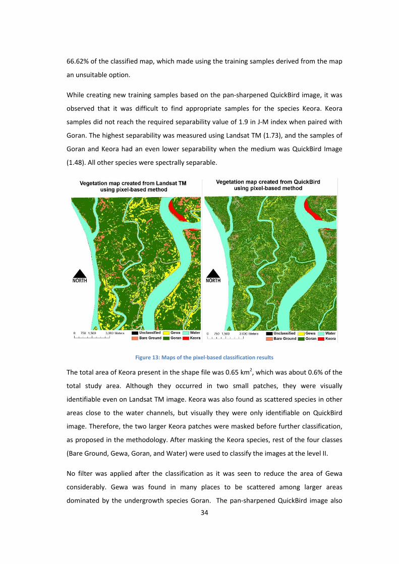
34
66.62% of the classified map, which made using the training samples derived from the map
an unsuitable option.
While creating new training samples based on the pan-sharpened QuickBird image, it was
observed that it was difficult to find appropriate samples for the species Keora. Keora
samples did not reach the required separability value of 1.9 in J-M index when paired with
Goran. The highest separability was measured using Landsat TM (1.73), and the samples of
Goran and Keora had an even lower separability when the medium was QuickBird Image
(1.48). All other species were spectrally separable.
Figure 13: Maps of the pixel-based classification results
The total area of Keora present in the shape file was 0.65 km2, which was about 0.6% of the
total study area. Although they occurred in two small patches, they were visually
identifiable even on Landsat TM image. Keora was also found as scattered species in other
areas close to the water channels, but visually they were only identifiable on QuickBird
image. Therefore, the two larger Keora patches were masked before further classification,
as proposed in the methodology. After masking the Keora species, rest of the four classes
(Bare Ground, Gewa, Goran, and Water) were used to classify the images at the level II.
No filter was applied after the classification as it was seen to reduce the area of Gewa
considerably. Gewa was found in many places to be scattered among larger areas
dominated by the undergrowth species Goran. The pan-sharpened QuickBird image also
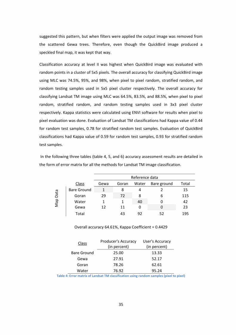
35
suggested this pattern, but when filters were applied the output image was removed from
the scattered Gewa trees. Therefore, even though the QuickBird image produced a
speckled final map, it was kept that way.
Classification accuracy at level II was highest when QuickBird image was evaluated with
random points in a cluster of 5x5 pixels. The overall accuracy for classifying QuickBird image
using MLC was 74.5%, 95%, and 98%, when pixel to pixel random, stratified random, and
random testing samples used in 5x5 pixel cluster respectively. The overall accuracy for
classifying Landsat TM image using MLC was 64.5%, 83.5%, and 88.5%, when pixel to pixel
random, stratified random, and random testing samples used in 3x3 pixel cluster
respectively. Kappa statistics were calculated using ENVI software for results when pixel to
pixel evaluation was done. Evaluation of Landsat TM classifications had Kappa value of 0.44
for random test samples, 0.78 for stratified random test samples. Evaluation of QuickBird
classifications had Kappa value of 0.59 for random test samples, 0.93 for stratified random
test samples.
In the following three tables (table 4, 5, and 6) accuracy assessment results are detailed in
the form of error matrix for all the methods for Landsat TM image classification.
Reference data
Ma
p D
ata
Class Gewa Goran Water Bare ground Total
Bare Ground 1 8 4 2 15
Goran 29 72 8 6 115
Water 1 1 40 0 42
Gewa 12 11 0 0 23
Total
43 92 52 195
Overall accuracy 64.61%, Kappa Coefficient = 0.4429
Class Producer's Accuracy
(in percent)
User's Accuracy
(in percent)
Bare Ground 25.00 13.33
Gewa 27.91 52.17
Goran 78.26 62.61
Water 76.92 95.24 Table 4: Error matrix of Landsat TM classification using random samples (pixel to pixel)

36
Reference data
Class Bare Ground Gewa Goran Water Total
Ma
p D
ata
Bare Ground 5 1 1 1 8
Gewa 0 31 0 1 32
Goran 3 11 92 5 111
Water 0 0 0 45 45
Total 8 43 93 52 196
Overall accuracy 88.26%
Class Producer's Accuracy
(in percent)
User's Accuracy
(in percent)
Bare Ground 62.50 62.50
Gewa 72.09 96.88
Goran 98.92 82.88
Water 86.54 100.00
Table 5: Error matrix of Landsat TM classification using random samples (3x3 cluster)
Reference data
Class Bare Ground Gewa Goran Water Total
Ma
p D
ata
Bare Ground 36 0 2 3 41
Gewa 0 44 3 0 47
Goran 14 6 45 5 70
Water 0 0 0 42 42
Total 50 50 50 50 200
Overall accuracy 83.05%, Kappa Coefficient = 0.7800
Class Producer's Accuracy
(in percent)
User's Accuracy
(in percent)
Bare Ground 72.00 87.80
Gewa 88.00 93.62
Goran 90.00 64.29
Water 84.00 100.00
Table 6: Error matrix of Landsat TM classification using stratified random samples (pixel to pixel)
In the following three tables (table 7, 8, and 9) accuracy assessment results are detailed in
the form of error matrix for QuickBird image classification.

37
Reference data
Class Bare Ground Gewa Goran Water Total
Ma
p D
ata
Bare Ground 4 0 5 2 11
Gewa 0 11 5 0 16
Goran 0 32 82 1 115
Water 4 0 1 49 54
Total 8 43 93 52 196
Overall accuracy 74.49%, Kappa Coefficient = 0.5940
Class Producer's Accuracy
(in percent)
User's Accuracy
(in percent)
Bare Ground 50.00 36.36
Gewa 25.58 68.75
Goran 88.17 71.30
Water 94.23 90.74
Table 7: Error matrix of QuickBird classification using random samples (pixel to pixel)
Reference data
Class Bare Ground Gewa Goran Water Total
Ma
p D
ata
Bare Ground 8 0 0 0 8
Gewa 0 39 0 0 39
Goran 0 4 93 0 97
Water 0 0 0 52 52
Total 8 43 93 52 196
Overall accuracy 97.96%
Class Producer's Accuracy
(in percent)
User's Accuracy
(in percent)
Bare Ground 100 100
Gewa 90.69 100
Goran 100 95.87
Water 100 100
Table 8: Error matrix of QuickBird classification using random samples (5x5 cluster)
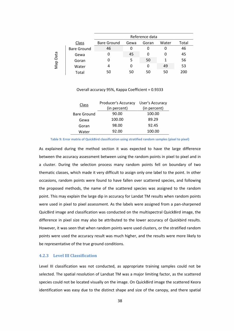
38
Reference data
Class Bare Ground Gewa Goran Water Total
Ma
p D
ata
Bare Ground 46 0 0 0 46
Gewa 0 45 0 0 45
Goran 0 5 50 1 56
Water 4 0 0 49 53
Total 50 50 50 50 200
Overall accuracy 95%, Kappa Coefficient = 0.9333
Class Producer's Accuracy
(in percent)
User's Accuracy
(in percent)
Bare Ground 90.00 100.00
Gewa 100.00 89.29
Goran 98.00 92.45
Water 92.00 100.00
Table 9: Error matrix of QuickBird classification using stratified random samples (pixel to pixel)
As explained during the method section it was expected to have the large difference
between the accuracy assessment between using the random points in pixel to pixel and in
a cluster. During the selection process many random points fell on boundary of two
thematic classes, which made it very difficult to assign only one label to the point. In other
occasions, random points were found to have fallen over scattered species, and following
the proposed methods, the name of the scattered species was assigned to the random
point. This may explain the large dip in accuracy for Landat TM results when random points
were used in pixel to pixel assessment. As the labels were assigned from a pan-sharpened
QuicBird image and classification was conducted on the multispectral QuickBird image, the
difference in pixel size may also be attributed to the lower accuracy of Quickbird results.
However, it was seen that when random points were used clusters, or the stratified random
points were used the accuracy result was much higher, and the results were more likely to
be representative of the true ground conditions.
4.2.3 Level III Classification
Level III classification was not conducted, as appropriate training samples could not be
selected. The spatial resolution of Landsat TM was a major limiting factor, as the scattered
species could not be located visually on the image. On QuickBird image the scattered Keora
identification was easy due to the distinct shape and size of the canopy, and there spatial

39
association with waterways. Bean was difficult to identified, but on pan-sharpened image it
was possible to identify them with much difficulties. However, separating the Dhundhul
and Passur was not possible even using the pan-sharpened QuickBird image.
When training samples were collected, Baen was collected separately but it was not
possible to separate the classes spectrally. After adding the combination of Dhundhul and
Passur, it was also not possible to spectrally separate them from other classes.
4.2.4 Significance of the Infrared bands
The overall accuracy of the Landsat TM classification without using the middle infrared
bands was 64.1% when random test samples were used to evaluate the result, and 78.5%
when stratified random samples were used to evaluate. The values achieved are slightly
lower than that of the accuracy values when classification was done including the middle
infrared bands. The difference between classifications with and without the middle infrared
bands was insignificant (0.4%) evaluated using the random samples, and small (5%)
stratified random samples were used to test accuracy.
4.3 Object-based classification
4.3.1 Scale level
For classification at level I it was found that optimum scale level was 85 for Landsat, and 65
for QuickBird to separate forest from water. However, analysis for finding the right scale
level at classification level II failed to find an appropriate value. None of the scale levels
satisfied the preset criteria of achieving a value of higher than 1.9 in J-M index denoting
good separability between the classes. A forward rotation texture analysis was made and
the output bands were stacked with the QuickBird image. The inclusion of texture as a
synthetic band improved the separability scores, but still failed to carry it above 1.9 in J-M
index.
It was found that the vegetation species are most separable at different scale levels. For
QuickBird, the optimum level for Gewa from Goran was at 25, Gewa from Keora was at 40,
and Goran from Keora was at 30). In case of the Landsat TM image the optimum
separability for Gewa from Keora was at 15 (values were very close all through from scale
level 10 to 30), Gewa from Goran, and Goran from Keora both was optimally separable at
scale level 30. At scale level 30 all species were optimally separable for both Landsat TM
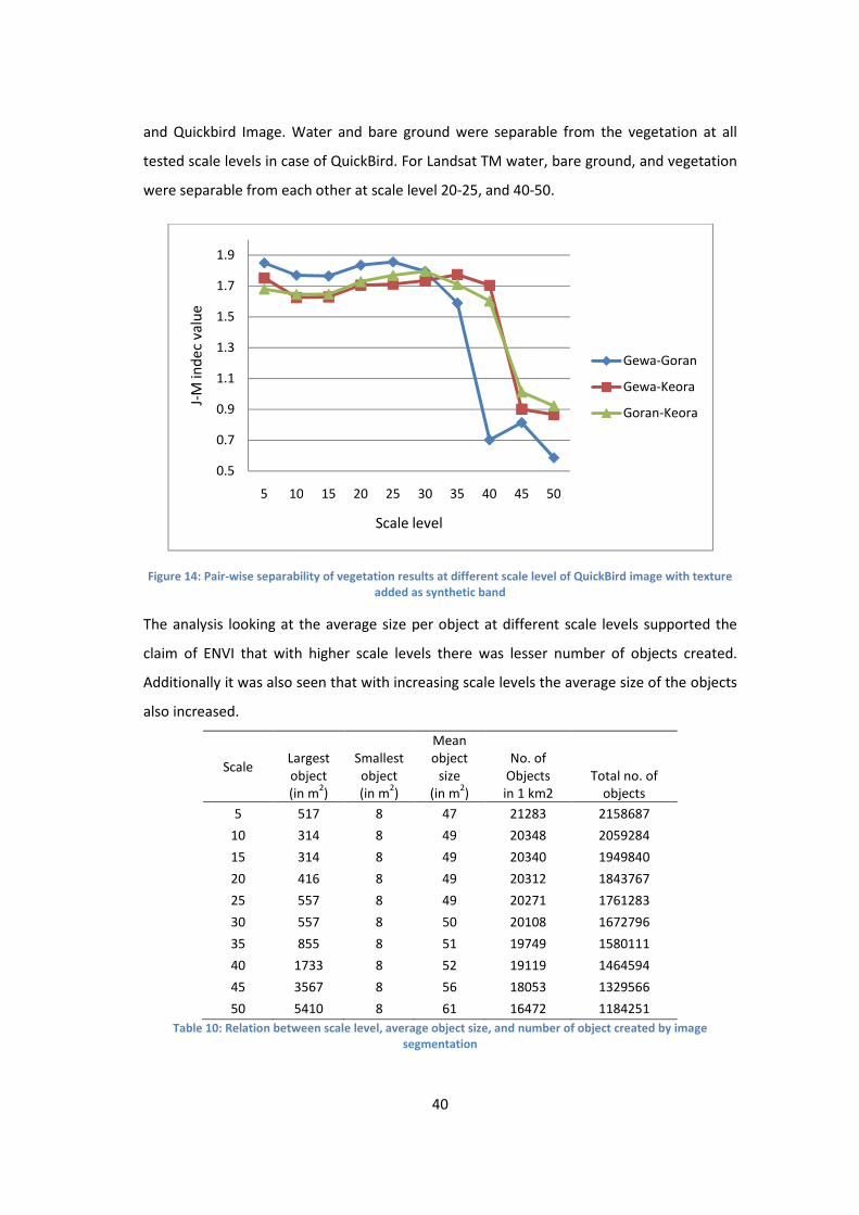
40
and Quickbird Image. Water and bare ground were separable from the vegetation at all
tested scale levels in case of QuickBird. For Landsat TM water, bare ground, and vegetation
were separable from each other at scale level 20-25, and 40-50.
Figure 14: Pair-wise separability of vegetation results at different scale level of QuickBird image with texture
added as synthetic band
The analysis looking at the average size per object at different scale levels supported the
claim of ENVI that with higher scale levels there was lesser number of objects created.
Additionally it was also seen that with increasing scale levels the average size of the objects
also increased.
Scale Largest
object
(in m2)
Smallest
object
(in m2)
Mean
object
size
(in m2)
No. of
Objects
in 1 km2
Total no. of
objects
5 517 8 47 21283 2158687
10 314 8 49 20348 2059284
15 314 8 49 20340 1949840
20 416 8 49 20312 1843767
25 557 8 49 20271 1761283
30 557 8 50 20108 1672796
35 855 8 51 19749 1580111
40 1733 8 52 19119 1464594
45 3567 8 56 18053 1329566
50 5410 8 61 16472 1184251
Table 10: Relation between scale level, average object size, and number of object created by image
segmentation
0.5
0.7
0.9
1.1
1.3
1.5
1.7
1.9
5 10 15 20 25 30 35 40 45 50
J-M
ind
ec
valu
e
Scale level
Gewa-Goran
Gewa-Keora
Goran-Keora
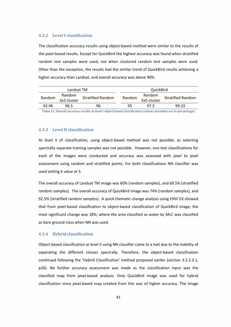
41
4.3.2 Level I classification
The classification accuracy results using object-based method were similar to the results of
the pixel-based results. Except for QuickBird the highest accuracy was found when stratified
random test samples were used, not when clustered random test samples were used.
Other than the exception, the results had the similar trend of QuickBird results achieving a
higher accuracy than Landsat, and overall accuracy was above 90%.
Landsat TM QuickBird
Random Random
3x3 cluster Stratified Random
Random
Random
5x5 cluster Stratified Random
92.96 96.5 96 95 97.5 99.33
Table 11: Overall accuracy results at level I object-based classification (values provided are in percentage)
4.3.3 Level II classification
At level II of classification, using object-based method was not possible, as selecting
spectrally separate training samples was not possible. However, one test classifications for
each of the images were conducted and accuracy was assessed with pixel to pixel
assessment using random and stratified points. For both classifications NN classifier was
used setting k value at 3.
The overall accuracy of Landsat TM image was 60% (random samples), and 69.5% (stratified
random samples). The overall accuracy of QuickBird image was 74% (random samples), and
92.5% (stratified random samples). A quick thematic change analysis using ENVI EX showed
that from pixel-based classification to object-based classification of QuickBird image, the
most significant change was 18%; where the area classified as water by MLC was classified
as bare ground class when NN was used.
4.3.4 Hybrid classification
Object-based classification at level II using NN classifier came to a halt due to the inability of
separating the different classes spectrally. Therefore, the object-based classification
continued following the 'Hybrid Classification' method proposed earlier (section 3.3.3.3.1,
p26). No further accuracy assessment was made as the classification input was the
classified map from pixel-based analysis. Only QuickBird image was used for hybrid
classification since pixel-based map created from this was of higher accuracy. The image
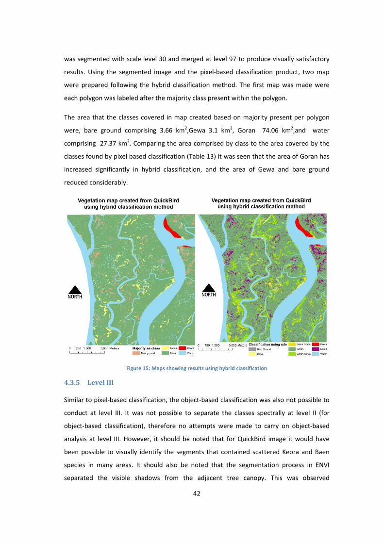
42
was segmented with scale level 30 and merged at level 97 to produce visually satisfactory
results. Using the segmented image and the pixel-based classification product, two map
were prepared following the hybrid classification method. The first map was made were
each polygon was labeled after the majority class present within the polygon.
The area that the classes covered in map created based on majority present per polygon
were, bare ground comprising 3.66 km2,Gewa 3.1 km2, Goran 74.06 km2,and water
comprising 27.37 km2. Comparing the area comprised by class to the area covered by the
classes found by pixel based classification (Table 13) it was seen that the area of Goran has
increased significantly in hybrid classification, and the area of Gewa and bare ground
reduced considerably.
Figure 15: Maps showing results using hybrid classification
4.3.5 Level III
Similar to pixel-based classification, the object-based classification was also not possible to
conduct at level III. It was not possible to separate the classes spectrally at level II (for
object-based classification), therefore no attempts were made to carry on object-based
analysis at level III. However, it should be noted that for QuickBird image it would have
been possible to visually identify the segments that contained scattered Keora and Baen
species in many areas. It should also be noted that the segmentation process in ENVI
separated the visible shadows from the adjacent tree canopy. This was observed
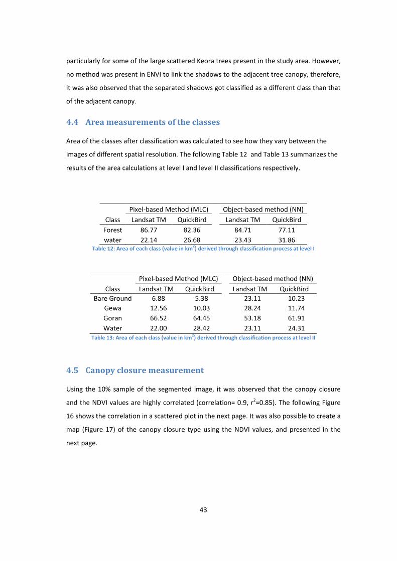
43
particularly for some of the large scattered Keora trees present in the study area. However,
no method was present in ENVI to link the shadows to the adjacent tree canopy, therefore,
it was also observed that the separated shadows got classified as a different class than that
of the adjacent canopy.
4.4 Area measurements of the classes
Area of the classes after classification was calculated to see how they vary between the
images of different spatial resolution. The following Table 12 and Table 13 summarizes the
results of the area calculations at level I and level II classifications respectively.
Pixel-based Method (MLC) Object-based method (NN)
Class Landsat TM QuickBird Landsat TM QuickBird
Forest 86.77 82.36 84.71 77.11
water 22.14 26.68 23.43 31.86 Table 12: Area of each class (value in km
2) derived through classification process at level I
Pixel-based Method (MLC) Object-based method (NN)
Class Landsat TM QuickBird Landsat TM QuickBird
Bare Ground 6.88 5.38 23.11 10.23
Gewa 12.56 10.03 28.24 11.74
Goran 66.52 64.45 53.18 61.91
Water 22.00 28.42 23.11 24.31
Table 13: Area of each class (value in km2) derived through classification process at level II
4.5 Canopy closure measurement
Using the 10% sample of the segmented image, it was observed that the canopy closure
and the NDVI values are highly correlated (correlation= 0.9, r2=0.85). The following Figure
16 shows the correlation in a scattered plot in the next page. It was also possible to create a
map (Figure 17) of the canopy closure type using the NDVI values, and presented in the
next page.

44
Figure 16: Relation between the canopy closure and NDVI values of the study area in a scatter plot
The visual interpretation of the canopy closure selecting up 30 samples to measure mean
NDVI values of each samples resulted in low canopy class ranging from 0.11 to 0.34 (mean
0.247), medium canopy class ranged from 0.38 to 0.56 (mean 0.495), and the high canopy
class ranged from 0.58 to 0.68 (mean 0.602).
Figure 17: Map of the three canopy classes based on NDVI value
R² = 0.8561
0
0.1
0.2
0.3
0.4
0.5
0.6
0.7
0.8
0 20 40 60 80 100
ND
VI
Canopy closure in percent
NDVI mean

45
5. Discussion
The objective of this research as introduced earlier was aimed at finding a suitable method
to classify the vegetation present in the Sundarban forest by comparing different
classification methods and EO data. Object-based classification technique and use of
Quickbird image for vegetation classification probably was a first for SRF through this study.
This research also proposed use of a hybrid method that is less resource intensive, easy to
implement, and flexible in terms of rules that can be used for classification. The hybrid
method can also provide higher attribute details for mixed classes in terms of exact
composition, area-wise contribution of different classes in each polygon, when compared
to the existing vector database developed using visual interpretation. The research also
verified the correlation of NDVI and vegetation of the study area, and developed the use of
NDVI values to classify canopy types present using the QuickBird image.
The analysis was conducted using Landsat TM and QuicBird images that were classified by
MLC, NN. The results obtained from theses analysis were found to be consistent with
previous studies conducted in Sundarban and elsewhere.
Figure 18: Comparison of the accuracy results at level I
The analysis was done at various classification levels, with increasing number of classes at
higher levels of classification. The results showed that with the increase of thematic details,
the accuracy of the classification decreased. However the rate of the diminishing accuracy
varied depending on the spatial resolution of the data, as Landsat TM results were of much
lower accuracy than that of Quickbird's (Figure 18 and Figure 19).
0
10
20
30
40
50
60
70
80
90
100
Random Cluster Stratified
Va
lue
in
% Landsat MLC
Landsat NN
QuickBird MLC
QuickBird NN
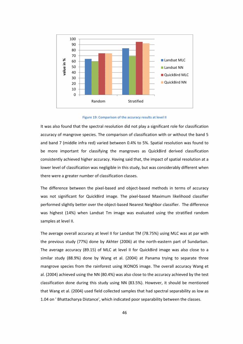
46
Figure 19: Comparison of the accuracy results at level II
It was also found that the spectral resolution did not play a significant role for classification
accuracy of mangrove species. The comparison of classification with or without the band 5
and band 7 (middle infra red) varied between 0.4% to 5%. Spatial resolution was found to
be more important for classifying the mangroves as QuickBird derived classification
consistently achieved higher accuracy. Having said that, the impact of spatial resolution at a
lower level of classification was negligible in this study, but was considerably different when
there were a greater number of classification classes.
The difference between the pixel-based and object-based methods in terms of accuracy
was not significant for QuickBird image. The pixel-based Maximum likelihood classifier
performed slightly better over the object-based Nearest Neighbor classifier. The difference
was highest (14%) when Landsat Tm image was evaluated using the stratified random
samples at level II.
The average overall accuracy at level II for Landsat TM (78.75%) using MLC was at par with
the previous study (77%) done by Akhter (2006) at the north-eastern part of Sundarban.
The average accuracy (89.15) of MLC at level II for QuickBird image was also close to a
similar study (88.9%) done by Wang et al. (2004) at Panama trying to separate three
mangrove species from the rainforest using IKONOS image. The overall accuracy Wang et
al. (2004) achieved using the NN (80.4%) was also close to the accuracy achieved by the test
classification done during this study using NN (83.5%). However, it should be mentioned
that Wang et al. (2004) used field collected samples that had spectral separability as low as
1.04 on ' Bhattacharya Distance', which indicated poor separability between the classes.
0
10
20
30
40
50
60
70
80
90
100
Random Stratified
va
lue
in
% Landsat MLC
Landsat NN
QuickBird MLC
QuickBird NN

47
Due to the limitations of not having spectrally separable training data, the classification
could not be carried out at level III. However, it was possible to create canopy closure
classes using NDVI values, as it was established that NDVI and canopy closures are highly
correlated. It was possible to conduct canopy measurements for both pixel-based and
object-based classification result. For pixel-based it could be left as individual pixel to
represent canopy type, and it makes more sense to do so for image like Landsat with larger
pixel size. For QuickBird or other for object-based results canopy type can be represented
per polygon with the average NDVI value of all the pixels present within that of a polygon.
Averaging the NDVI value per polygon is useful in case of images with spatially very small
pixel size, because it was seen during the analysis that large trees are comprised of many
pixels in the QuickBird scene. Therefore it makes sense to consider a tree canopy as a single
polygon with a single canopy type value assigned, as logically one tree cannot have more
than one canopy type.
The scale of the image played an important role on the classification results, as at all times
the area of the classes where different comparing Landsat TM results to QuickBird results.
QuickBird image classification at all stages produced more area for water than Landsat TM
image outputs. This can be explained by the spatial resolution difference of the data type.
Since the QuickBird has a much higher spatial resolution, visually more water channels
were identifiable on it, than in Landsat TM image. In many areas the small narrow water
channels surrounded by trees were absent in Landsat TM image due to the larger pixel size.
Those same narrow channels were clearly identifiable on QuickBird image due to its much
finer spatial resolution.
Based on the area per class results (Table 12 and Table 13), it was also found that the
object-based classification were more suited for QuickBird image at all levels of
classification; as difference noticed was not significant comparing results of pixel and object
based methods. At classification level II object-based method reported more bare-ground
area than the pixel-based results and less area of water than pixel-based results. This issue
could be attributed to the temporal context of image acquisition. As mentioned in the data
and results section, the QuickBird image may have been acquired during the high tide
which resulted temporal flooding of the forest floor that is visible in the data. The presence
of water inside the forest may have caused the area to be classified as water using MLC
classifier and same area may have been classified as bare ground using object-based
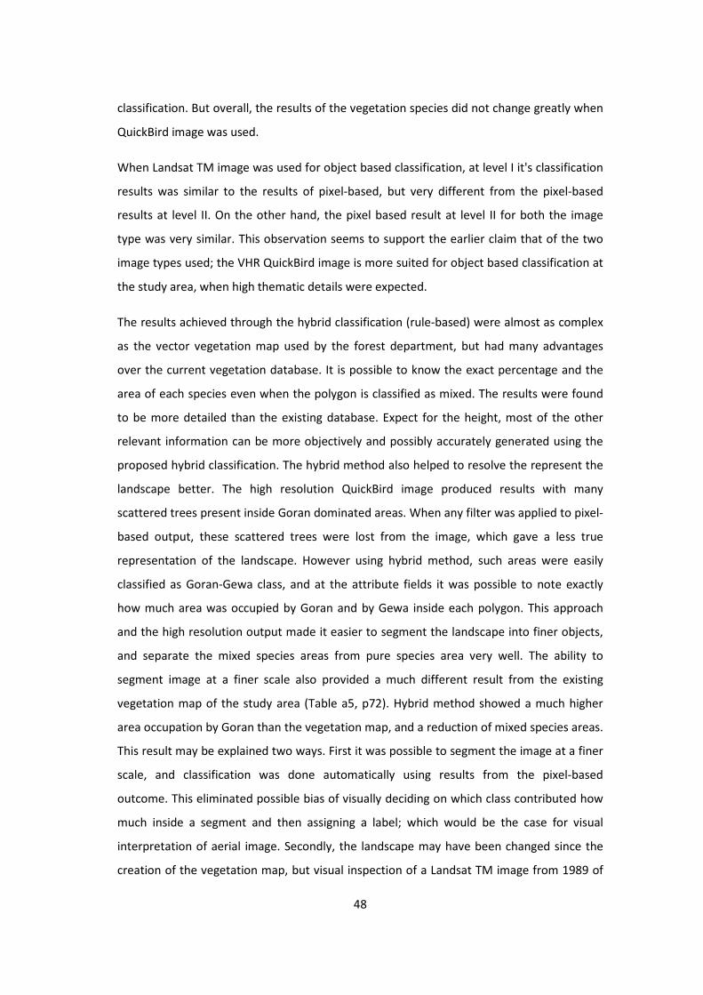
48
classification. But overall, the results of the vegetation species did not change greatly when
QuickBird image was used.
When Landsat TM image was used for object based classification, at level I it's classification
results was similar to the results of pixel-based, but very different from the pixel-based
results at level II. On the other hand, the pixel based result at level II for both the image
type was very similar. This observation seems to support the earlier claim that of the two
image types used; the VHR QuickBird image is more suited for object based classification at
the study area, when high thematic details were expected.
The results achieved through the hybrid classification (rule-based) were almost as complex
as the vector vegetation map used by the forest department, but had many advantages
over the current vegetation database. It is possible to know the exact percentage and the
area of each species even when the polygon is classified as mixed. The results were found
to be more detailed than the existing database. Expect for the height, most of the other
relevant information can be more objectively and possibly accurately generated using the
proposed hybrid classification. The hybrid method also helped to resolve the represent the
landscape better. The high resolution QuickBird image produced results with many
scattered trees present inside Goran dominated areas. When any filter was applied to pixel-
based output, these scattered trees were lost from the image, which gave a less true
representation of the landscape. However using hybrid method, such areas were easily
classified as Goran-Gewa class, and at the attribute fields it was possible to note exactly
how much area was occupied by Goran and by Gewa inside each polygon. This approach
and the high resolution output made it easier to segment the landscape into finer objects,
and separate the mixed species areas from pure species area very well. The ability to
segment image at a finer scale also provided a much different result from the existing
vegetation map of the study area (Table a5, p72). Hybrid method showed a much higher
area occupation by Goran than the vegetation map, and a reduction of mixed species areas.
This result may be explained two ways. First it was possible to segment the image at a finer
scale, and classification was done automatically using results from the pixel-based
outcome. This eliminated possible bias of visually deciding on which class contributed how
much inside a segment and then assigning a label; which would be the case for visual
interpretation of aerial image. Secondly, the landscape may have been changed since the
creation of the vegetation map, but visual inspection of a Landsat TM image from 1989 of

49
the study area suggests this to be less likely. In absence of detailed attribute data in the
vector file of the vegetation it was hard to comment why exactly such large differences has
occurred between the results from this study and the existing vegetation map.
One potential limitation was found about the way the ENVI software segments the image.
As seen from the results (Table 10, p40) and also from the documentation accompanying
the ENVI software that scale levels and the number of object created through the
segmentation process are inversely related. It was also seen (Table 10) that the increase in
scale level on an average causes the objects to be larger. However it was also seen that
(Figure 14, p40) the vegetation species are optimally separable from each other at different
scale level, but for segmenting the image only one scale level value can be selected. The
implications are that at different scale, different sized objects are created, and that may
explain why the vegetation species are better separated at different scale. Personal
experience suggests that the three species present at the study have different size, shape
and height of canopy. Chances are there that this probably is a driving factor for
segmentation, as well as, for separability. However, due to a lack of available literature on
how exactly ENVI performs the segmentation based on scale parameter; it was not possible
to make a concrete statement on this.
It will not be irrelevant to comment that it was felt that more could have been done with
object based classification using the QuickBird image. Other object based classification and
image segmentation techniques, and good ground data in the future may help to establish
better results. It was felt that other form of information, such as additional height data,
association of vegetation species with water, association of shadow with adjacent tree may
help to better discriminate between the classes. For example, during visual inspection it
was possible to identify many scattered trees easily because of their familiar shape and
proximity to water channels, but it was not possible to translate such information to the
inbuilt classifier in the software used. Shadows were also helpful cognitively to identify
taller tree stands, which aided a better separability of the vegetation classes during
exploratory analysis. Therefore it was thought that future studies including height data of
the trees can help the vegetation classification at the study area.
As mentioned in the result in some cases the shadow of the tree falling on a second species
was identified as a third species. Due to the limitation of the timeframe allowed for the
current research it was not possible to investigate using other classifiers that are capable of

50
knowledge-based classification. Future studies may be conducted to investigate this issue.
Using pan-sharpened image to be used for object-based classification for the study area
also remains to be investigated in the future.
5.1 Discussion on research questions
1. What is a better classification method for classifying the mangrove species in SRF, pixel-
based or object-based?
Pixel-based methods performed slightly better than the object-based methods based
on accuracy results. However, when used with VHR data hybrid object based method
may provide greater flexibility.
2. Does the use of VHR EO product help to achieve results with higher accuracy?
Yes, high spatial resolution QuickBird data consistently produced better results.
3. What is the extent of thematic details possible to attain for vegetation maps of the
study area using different EO data?
Following the methods of this study it was possible to classify the RS images up to
classification level II. Landsat TM probably has the potential to be classified only up to
level II, as it was not possible to identify the scattered vegetation beyond the large
zones of dominant vegetation species.
For QuickBird images it was felt that even though under this study design it was
classified till level II, but with pan-sharpened image and adequate field data it may be
possible to classify the image with more thematic details than Landsat TM image. It was
possible to identify the scattered trees with large canopies even in the multispectral
QuickBird image, but there was not enough spectral difference found for them to be
classified accurately under the methods followed.
5.2 Discussion on null hypotheses
With the results presented and discussion made, the following null hypotheses can be said
to have been successfully rejected.
1. All methods are equally accurate to classify the vegetation of Sundarban reserved
forest (SRF)
2. EO data of SRF with different scales will produce vegetation classification results of
same accuracy
51
6. Conclusion
It was found through this research that different remote sensing methods and EO data of
different scales of Sundarban Reserve Forest will produce classification results of varying
degrees of accuracy. The question of which data and method is more suited to the study
area remained as a context related issue, as both data types and methods produced similar
results in most stages of the analysis. However, it must be mentioned that using VHR data
constantly produced higher accuracy, especially when higher thematic details where
required. Neither of the data types or the different methods could be used at highest level
of thematic details following the proposed methodology of the current study. Therefore
further study with adequate ground verification data is required to make any definitive
remark on what is the highest level output possible from the VHR EO data in SRF.
It was found that the object-based hybrid method provides greater flexibility for
classification. This method can be used with simple majority rule to complex rules of
species mixture with defined quantities. Results found from the hybrid classification using
the same rules used to construct the vegetation database used by the Bangladesh Forest
Department, were found to have a much detailed representation than the existing
vegetation maps. The method also provides more information about each class and their
composition, compared to the more subjective photo interpreted results.
The object-based method was found more suitable for the VHR data, and was almost as
accurate as pixel-based method when used with QuickBird image, but produced lower
accuracy when used with Landsat TM image. Both images were found to produce more
accurate results when pixel-based method was used.
Scale of the data played a greater role when object based method was implemented, and
also when more classes were being indentified using pixel-based method. Spatial resolution
was found to be more important for accurate classification of the mangrove species of the
study area than spectral resolution. NDVI was found to be highly related with canopy
closure of the study area, and can be used to create vegetation canopy classification.
Finally it can be said that the current research, albeit limitations, was able to fulfill the
objectives by answering the research question asked, following the methods proposed.

52
6.1 Limitations
1. Lack of ground verification was thought to be the biggest limitation for this study. It
was not possible to visit the study area due to limited timeframe and lack of
sufficient funds. The vegetation map initially hoped to be used as ground
verification was not detailed enough for verifying the results of VHR data.
2. Shadows present in Quickbird were seen to be improperly classified in some cases.
3. ENVI Zoom/EX produced large datasets when lower scale level was used and
working with those large dataset was computationally intensive.
4. Personal limitations in terms of lack of in-depth knowledge of alternative remote
sensing techniques.
6.2 Recommendation for future studies
1. Further studies including field visit is recommended to firmly establish the findings
from this studies. Pan-sharpened VHR data is to be used to see if it may be used for
classifying vegetation of the study area with higher thematic details.
2. Different software and algorithm for object-based classification may be used to see
if they improve the classification results further.
3. Further studies on individual species canopy cover and their relation with NDVI
needs to be investigated. If all the species responds with the similar strong relation
found during this study, then NDVI can be used effectively to monitor the change of
vegetation density in Sundarban over time.

53
Bibliographic Reference
AGRAWALA, S., OTA, T., AHMED, A. U., SMITH, J. & AALST, M. V. 2003. Development And
Climate Change In Bangladesh: Focus On Coastal Flooding And The Sundarbans.
Paris: Organisation for Economic Co-operation and Development (OECD).
AHMED, A. U., SIDDIQI, N. A. & CHOUDHURI, R. A. 1998. Vulnerability of Forest Ecosystems
of Bangladesh to Climate change. In: HUQ, S., KARIM, Z., ASADUZZAMAN, M. &
MAHTAB, F. (eds.) Vulnerability and adaptation to Climate Change for Bangladeh.
Dordrecht /Boston /London: Kluwer Academic Publishers.
AKHTER, M. 2006. Remote sensing for developing an operational monitoring scheme for the
Sundarban Reserved Forest, Bangladesh. Doctor of Natural Science Dr. rer. nat.,
Technische Universität Dresden.
AKHTER, M., MOHAIMAN, R. & ALAM, M. 2002. Forest Types : Sheet 2, Scale 1:25000.
Dhaka Bangladesh Forest Department.
ALAM, M. M. 2008. Monitoring Changes in Sundarbans Mangrove Forest Based on the
Analysis of Landsat Images. Master of Forest Information Technology, University of
Applied Sciences Eberswalde.
ANGERER, A. & MARCOLONGO, B. Forest cover analysis with multitemporal and
multispectral images a case study in the dolomites(Northern Italy). Pecora 16:
Global Priorities in Land Remote Sensing, 2005 Sioux Falls, South Dakota. American
Society for Photogrammetry and Remote Sensing.
BEERI, O., PHILLIPS, R., HENDRICKSON, J., FRANK, A. B. & KRONBERG, S. 2007. Estimating
forage quantity and quality using aerial hyperspectral imagery for northern mixed-
grass prairie. Remote Sensing of Environment, 110, 216-225.
BIAN, L. 2007. Object-Oriented Representation of Environmental Phenomena: Is Everything
Best Represented as an Object? Annals of the Association of American
Geographers, 97, 267 - 281.
BLASCO, F., AIZPURU, M. & NDONGO, D. D. 2005. Mangroves, Remote Sensing.
Encyclopedia of Coastal Science.
CAMPBELL, J. B. 2002a. Digital Data. Introduction to remote sensing. 3rd ed. London: Taylor
& Francis.
CAMPBELL, J. B. 2002b. Image Classification. Introduction to remote sensing. 3rd ed.
London: Taylor & Francis.
CAMPBELL, J. B. 2002c. Plant Science. Introduction to remote sensing. 3rd ed. London:
Taylor & Francis.
CAMPBELL, J. B. 2002d. Preprocessing. Introduction to remote sensing. 3rd ed. London:
Taylor & Francis.

54
CCRS 2007. Fundamentals of Remote Sensing. A Canada Centre for Remote Sensing Remote
Sensing Tutorial. Canada Centre for Remote Sensing.
CHAFFEY, D. R., MILLER, F. R. & SANDOM, J. H. 1985. A forest inventory of the Sundarban,
Bangladesh. Surbiton, Surrey: Overseas Development Administration.
CHOWDHURY, K. 15 dec 2010 2010. RE: Telephone conversation regarding presence of
grassland near Notabeki forest station. Type to DIYAN, M. A. A.
CHOWDHURY, R. A. & AHMED, I. 1994. History of Forest Management. In: HUSSAIN, Z. &
ACHARYA, G. (eds.) Mangroves of the Sundarbans. Volume two : Bangladesh.
Bangkok: IUCN.
CONGALTON, R. G. & GREEN, K. 2009a. Chapter 4 Thematic Accuracy. Assessing the
Accuracy of Remotely Sensed Data. 2nd ed. Boca Raton: CRC Press.
CONGALTON, R. G. & GREEN, K. 2009b. Chapter 5 Sample Design Considerations. Assessing
the Accuracy of Remotely Sensed Data. 2nd ed. Boca Raton: CRC Press.
COUCLELIS, H. 1992. People manipulate objects (but cultivate fields): Beyond the raster-
vector debate in GIS. Theories and Methods of Spatio-Temporal Reasoning in
Geographic Space. Springer Berlin / Heidelberg.
DAHDOUH-GUEBAS, F., VAN HIEL, E., CHAN, J. C. W., JAYATISSA, L. P. & KOEDAM, N. 2004.
Qualitative distinction of congeneric and introgressive mangrove species in mixed
patchy forest assemblages using high spatial resolution remotely sensed imagery
(IKONOS). Systematics and Biodiversity, 2, 113-119.
DIGITALGLOBE. 2004. GLCF: Digitalglobe Quickbird Imagery [Online]. Longmont:
DigitalGlobe. Available:
http://www.glcf.umd.edu/data/quickbird/sundarbans.shtml [Accessed 15 Sep
2010].
DIGITALGLOBE. 2010. DigitalGlobe | DigitalGlobe: QuickBird Satellite - 60cm Resolution
[Online]. Available: http://www.digitalglobe.com/index.php/85/QuickBird
[Accessed 24 April 2010].
ELLISON, A. M., MUKHERJEE, B. B. & KARIM, A. 2000. Testing patterns of zonation in
mangroves: scale dependence and environmental correlates in the Sundarbans of
Bangladesh. Journal of Ecology, 88, 813-824.
EMCH, M. & PETERSON, M. 2006. Mangrove Forest Cover Change in the Bangladesh
Sundarbans from 1989-2000: A Remote Sensing Approach. Geocarto International,
21, 5 - 12.
ENVI 2008. ENVI Feature Extraction Module User’s Guide. Feature Extraction Module
Version 4.6 December, 2008 Edition. ITT Visual Information Solutions.
GIRI, C., PENGRA, B., ZHU, Z., SINGH, A. & TIESZEN, L. L. 2007. Monitoring mangrove forest
dynamics of the Sundarbans in Bangladesh and India using multi-temporal satellite
data from 1973 to 2000. Estuarine, Coastal and Shelf Science, 73, 91 - 100.

55
GOODCHILD, M. F. 1994. Integrating GIS and remote sensing for vegetation analysis and
modeling: methodological issues. Journal of Vegetation Science, 5, 615-626.
GREEN, E. P., CLARK, C. D., MUMBY, P. J., EDWARDS, A. I. & ELLIS, A. C. 1998. Remote
sensing techniques for mangrove mapping. International Journal of Remote
Sensing, 19, 935-956.
HUSSAIN, Z. & AHMED, I. 1994. Management of the forest resources. In: HUSSAIN, Z. &
ACHARYA, G. (eds.) Mangroves of the Sundarbans. Volume two : Bangladesh.
Bangkok: IUCN.
HUSSAIN, Z. & KARIM, A. 1994. Introduction. In: HUSSAIN, Z. & ACHARYA, G. (eds.)
Mangroves of the Sundarbans. Volume two : Bangladesh. Bangkok: IUCN.
IFTEKHAR, M. S. & ISLAM, D. M. R. 2002. Vegetation Dynamics in The Sundarbans and its
Implication on The Integrated Coastal Zone Management of Bangladesh. Dhaka:
Program Development Office for Integrated Coastal Zone Management (PDO-
ICZM).
IPCC 2002. Climate Change and Biodiversity. In: GITAY, H., SUAREZ, A., WATSON, R. T. &
DOKKEN, D. J. (eds.) IPCC Technical Paper V. Intergovernmental Panel On Climate
Change.
ISLAM, M. J., ALAM, M. S. & ELAHI, K. M. 1997. Remote sensing for change detection in the
Sunderbands, Bangladesh. Geocarto International, 12, 91 - 100.
JENSEN, J. R., LIN, H., YANG, X., RAMSEY, E., DAVIS, B. A. & THOEMKE, C. W. 1991. The
measurement of mangrove characteristics in southwest Florida using spot
multispectral data. Geocarto International, 6, 13 - 21.
KANNIAH, K. D., WAI, N. S., SHIN, A. L. M. & RASIB, A. W. 2007. Per-pixel and sub-pixel
classifications of high-resolution satellite data for mangrove species mapping.
Applied GIS, 3, 1-22.
KARIM, A. 1994. Vegetation. In: HUSSAIN, Z. & ACHARYA, G. (eds.) Mangroves of the
Sundarbans. Volume two : Bangladesh. Bangkok: IUCN.
LANDGREBE, D. A. 2003. Introduction and Background. Signal theory methods in
multispectral remote sensing. Hoboken, New Jersey: John Wiley and Sons.
MANGROVE, F. O. 2009. World Mangrove Distribution [Online]. Selango: Friends of
Mangrove. Available:
http://www.friendsofmangrove.org.my/index.cfm?&menuid=10 [Accessed 7 Oct
2010].
NEUMANN-DENZAU, G. & DENZAU, H. 2010. Examining the Extent of Human-Tiger Conflict
in the Sundarbans Forest, Bangladesh. Tigerpaper 37, 4-7.
RAMSAR. 2007. Ramsar Sites Information Service [Online]. Available:
http://ramsar.wetlands.org/Database/Searchforsites/tabid/765/Default.aspx
[Accessed Oct 27 2008].

56
RICHARDS, J. A. & JIA, X. 2006a. Feature Reduction. Remote sensing digital image analysis:
an introduction. Verlag: Springer.
RICHARDS, J. A. & JIA, X. 2006b. Image Classification Methodologies. Remote sensing digital
image analysis: an introduction. Verlag: Springer.
RICHARDS, J. A. & JIA, X. 2006c. Sources and Characteristics of Remote Sensing Image Data.
Remote sensing digital image analysis: an introduction. Verlag: Springer.
ROBINSON, D. J., REDDING, N. J. & CRISP, D. J. 2002. Implementation of a fast algorithm for
segmenting SAR imagery. Scientific and Technical Report. Australia: Defense Science
and Technology Organization.
SYED, M. A., HUSSIN, Y. A. & WEIR, M. Detecting Fragmented Mangroves in the Sundarbans,
Bangladesh Using Optical and Radar Satellite Images. Asian Conference on Remote
Sensing, 5-9 Nov 2001 Singapore.
TOMLINSON, P. B. 1995. The Botany of Mangroves. Cambridge tropical biology series.
Cambridge [Cambridgeshire] ; New York: Cambridge University Press.
UNESCO. 1997. The Sundarbans - UNESCO World Heritage Centre [Online]. Available:
http://whc.unesco.org/en/list/798 [Accessed 27 Oct 2008].
USGS. 1999. Tri-Decadal Global Landsat Orthorectified Overview [Online]. Available:
http://eros.usgs.gov/#/Find_Data/Products_and_Data_Available/Tri-
Decadal_Global_Landsat_Orthorectified_Overview [Accessed 21 Jan 2011].
USGS. 2002. USGS Global Visualization Viewer [Online]. U.S. Geological Survey. Available:
http://glovis.usgs.gov/ [Accessed 15 Sep 2010].
USGS. 2004. Landsat 5 History [Online]. Available:
http://landsat.usgs.gov/about_landsat5.php [Accessed 21 Jan 2010].
USGS. 2009. Landsat Thematic Mapper Data (TM) [Online]. Available:
http://eros.usgs.gov/#tm6 [Accessed 25 Apr 2010].
WANG, L., SOUSA, W. P. & GONG, P. 2004. Integration of object-based and pixel-based
classification for mapping mangroves with IKONOS imagery. International Journal of
Remote Sensing, 25, 5655 - 5668.
XIE, Y., SHA, Z. & YU, M. 2008. Remote sensing imagery in vegetation mapping: a review.
Journal of Plant Ecology, 1, 9-23.

57
Appendices
58
A.1 Mean pixel values at different spectral bands for thematic
classes
In the following figures mean pixel value of each thematic class is presented for both
Landsat TM and QuickBird image of the study area. In the first figure (Figure a1)shows the
mean values of of the classes for the Landsat TM image. The band number in the horizontal
axis are the spectral bands of the Landsat TM image. Band 1 to Band 5 are the regular
bands of the image, band 6 represents band 7 of the actual Landsat TM band, and band 7 is
NDVI transformed to 8 bit and stacked as a synthetic band.
The second and third figure (Figure a2 & Figure a3) show the means pixel values of the
thematic classes across the spectral bands of QuickBird image. Figure a2 shows the values
for the four multi-spectral (MS) bands of QuickBird; and Figure a3 shows the four MS bands
and NDVI converted to 11bit as band 5.
Figure a1: Mean pixel values of the thematic classes across the spectral bands and NDVI (band 7) of Landsat
TM image of the study area

59
Figure a2: Mean pixel values of the thematic classes across the spectral bands of QuickBird image of the study
area
Figure a3: Mean pixel values of the thematic classes across the spectral bands and NDVI (band 5) of QuickBird
image of the study area

60
A.2 Visual interpretation consistency test results
The following three figures show the min/max/mean pixel values of the species Gewa
(Excoecaria agallocha) across the MS bands of QuickBird images. QuickBird images of the
two other areas in Sundarban forest were used to investigate the consistency of the visual
interpretation of the researcher. The first figure (Figure a4) represents the mean of the
pixel values of the training samples from the study area. The second figure (Figure a5)
represent values of Gewa from western part of the Sundarban forest situated north of the
study area (test site 1), and the last figure (Figure a6) has the mean pixel values of Gewa
present in the eastern part of the Sundarban forest (test site 2) . For details of how the
analysis was done please refer to Training samples generation (p23).
Figure a4: Mean pixel value of the training samples of the species Gewa (Excoecaria agallocha) of the study
area in QuickBird image
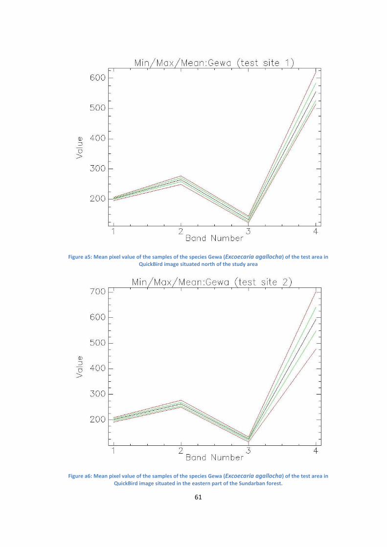
61
Figure a5: Mean pixel value of the samples of the species Gewa (Excoecaria agallocha) of the test area in
QuickBird image situated north of the study area
Figure a6: Mean pixel value of the samples of the species Gewa (Excoecaria agallocha) of the test area in
QuickBird image situated in the eastern part of the Sundarban forest.

62
A.3 Influence of NDVI in pair-wise separability result
The following tables (Table a, Table a2) summarize the results achieved using with or without
adding NDVI as a synthetic band to the image during pair-wise separability test. The
separability tests were conducted using the Jeffries- Matusita (J-M) index, where values
above 1.9 indicate good separability between the pairs. The first table shows the
differences in the pair-wise separability when a Landsat TM of the study area is used
without NDVI as a synthetic band and then when NDVI was stacked as a synthetic band. The
second table also shows the differences in pair-wise separability between using and not
using NDVI as a synthetic band stacked with the QuickBird image of the study area.
Without NDVI stacked as a synthetic band
Classes 1 2 3 4 5
1 Bare Ground 0
2 Gewa 2 0
3 Goran 2 1.948 0
4 Keora 1.999 1.995 1.584 0
5 Water 2 2 2 2 0
With NDVI stacked as a synthetic band
Classes 1 2 3 4 5
1 Bare Ground 0
2 Gewa 2 0
3 Goran 2.000 1.973 0
4 Keora 2.000 1.998 1.730 0
5 Water 2 2 2 2 0
Table a1: Result of pair-wise separability of the thematic classes using Landsat TM image with and without
NDVI as a synthetic band
Without NDVI stacked as a synthetic band
Classes 1 2 3 4 5
1 Bare Ground 0
2 Gewa 2 0
3 Goran 2.000 1.949 0
4 Keora 2.000 1.847 1.249 0
5 Water 1.998 2 2 2 0
With NDVI stacked as a synthetic band
Classes 1 2 3 4 5
1 Bare Ground 0
2 Gewa 2 0
3 Goran 2 1.985 0
4 Keora 2 1.952 1.437 0
5 Water 1.9998 2 2 2 0 Table a2: Result of pair-wise separability of the thematic classes using QuickBird image with and without
NDVI as a synthetic band

63
A.4 Separability results of QuickBird image at different scale levels
In the following tables and figures the results of pair-wised separability of the object-based
classification are depicted. The results are derived using in J-M index. At each different
scale level of segmentation process, the resultant segmented image with objects was
intersected with the training samples of the pixel-based method. Then each object was
treated as a sample and used for pair-wise separability test using QuickBird Image with
NDVI added as synthetic layer.
Scale 5
1 2 3 4 5
1 Bare Ground 0
2 Gewa 1.999255 0
3 Goran 1.983702 1.42825393 0
4 Keora 1.977539 1.50505961 1.3389912 0
5 Water 1.955277 1.99999999 1.999994 1.99998 0
Scale 10
1 2 3 4 5
1 Bare Ground 0
2 Gewa 1.999715 0
3 Goran 1.999006 1.3390657 0
4 Keora 1.994973 1.38377319 1.4164153 0
5 Water 1.981755 2.00000000 1.99999998 1.999999 0
Scale 15
1 2 3 4 5
1 Bare Ground 0
2 Gewa 1.999752 0
3 Goran 1.999102 1.32862583 0
4 Keora 1.996833 1.38772122 1.418958 0
5 Water 1.997647 2.00000000 2 2 0
Scale 20
1 2 3 4 5
1 Bare Ground 0
2 Gewa 1.999948 0
3 Goran 1.999439 1.45436402 0
4 Keora 1.997019 1.49793835 1.523816 0
5 Water 1.997125 2 2 2 0 Table a3: Pair-wise separability results of the thematic classes using QuickBird image at different scale levels
(Continued)

64
Scale 25
1 2 3 4 5
1 Bare Ground 0
2 Gewa 1.999976 0
3 Goran 1.999736 1.52509446 0
4 Keora 1.997789 1.50742797 1.5771627 0
5 Water 1.992508 2.00000000 2 2 0
Scale 30
1 2 3 4 5
1 Bare Ground 0
2 Gewa 1.999987 0
3 Goran 1.999823 1.58464302 0
4 Keora 1.997958 1.55582401 1.6297584 0
5 Water 1.987409 2.00000000 2 2 0
Scale 35
1 2 3 4 5
1 Bare Ground 0
2 Gewa 1.999993 0
3 Goran 1.999853 1.3948186 0
4 Keora 1.998007 1.61303255 1.5318983 0
5 Water 1.981197 2.00000000 2 2 0
Scale 40
1 2 3 4 5
1 Bare Ground 0
2 Gewa 1.999942 0
3 Goran 1.999883 0.54096477 0
4 Keora 1.99824 1.54341109 1.4052946 0
5 Water 1.97553 2.00000000 2 2 0
Table a3: Pair-wise separability results of the thematic classes using QuickBird image at different
scale levels
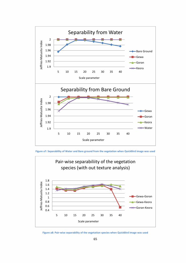
65
Figure a7: Separability of Water and Bare ground from the vegetation when QuickBird image was used
Figure a8: Pair-wise separability of the vegetation species when QuickBird image was used
1.9
1.92
1.94
1.96
1.98
2
5 10 15 20 25 30 35 40
Jeff
rie
s-M
atu
sita
In
de
x
Scale parameter
Separability from Water
Bare Ground
Gewa
Goran
Keora
1.9
1.92
1.94
1.96
1.98
2
5 10 15 20 25 30 35 40
Jeff
rie
s-M
atu
sita
In
de
x
Scale parameter
Separability from Bare Ground
Gewa
Goran
Keora
Water
0.4
0.6
0.8
1
1.2
1.4
1.6
1.8
5 10 15 20 25 30 35 40
Jeff
rie
s-M
atu
sita
In
de
x
Scale parameter
Pair-wise separabiliity of the vegetation
species (with out texture analysis)
Gewa-Goran
Gewa-Keora
Goran-Keora

66
Figure a9: Pair-wise separability results of the vegetation species showing the differences when texture co-
occurrence was added to QuickBird image during the analysis
0.5
0.7
0.9
1.1
1.3
1.5
1.7
1.9
5 10 15 20 25 30 35 40
Jeff
rie
s-M
atu
sita
In
de
x
Pair-wise separabiliity of Gewa-Goran
With texture
Without texture
0.5
0.7
0.9
1.1
1.3
1.5
1.7
1.9
5 10 15 20 25 30 35 40
Jeff
rie
s-M
atu
sita
In
de
x
Pair-wise separabiliity of Goran-Keora
With texture
Without texture
0.5
0.7
0.9
1.1
1.3
1.5
1.7
1.9
5 10 15 20 25 30 35 40
Jeff
rie
s-M
atu
sita
In
de
x
Pair-wise separabiliity of Gewa-Keora
With texture
Without texture
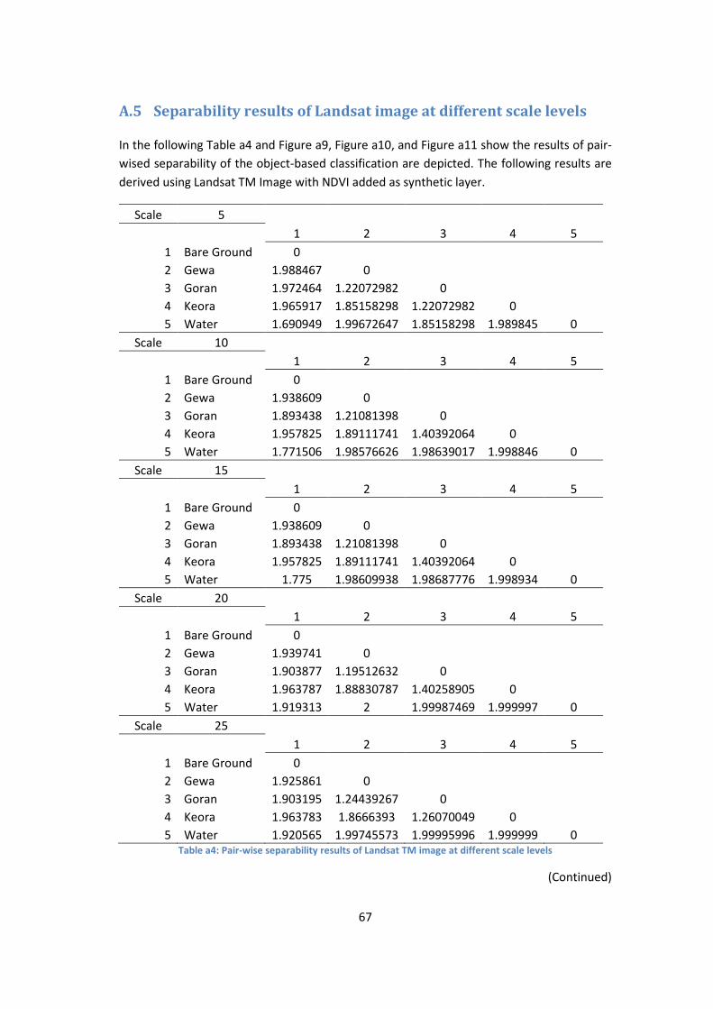
67
A.5 Separability results of Landsat image at different scale levels
In the following Table a4 and Figure a9, Figure a10, and Figure a11 show the results of pair-
wised separability of the object-based classification are depicted. The following results are
derived using Landsat TM Image with NDVI added as synthetic layer.
Scale 5
1 2 3 4 5
1 Bare Ground 0
2 Gewa 1.988467 0
3 Goran 1.972464 1.22072982 0
4 Keora 1.965917 1.85158298 1.22072982 0
5 Water 1.690949 1.99672647 1.85158298 1.989845 0
Scale 10
1 2 3 4 5
1 Bare Ground 0
2 Gewa 1.938609 0
3 Goran 1.893438 1.21081398 0
4 Keora 1.957825 1.89111741 1.40392064 0
5 Water 1.771506 1.98576626 1.98639017 1.998846 0
Scale 15
1 2 3 4 5
1 Bare Ground 0
2 Gewa 1.938609 0
3 Goran 1.893438 1.21081398 0
4 Keora 1.957825 1.89111741 1.40392064 0
5 Water 1.775 1.98609938 1.98687776 1.998934 0
Scale 20
1 2 3 4 5
1 Bare Ground 0
2 Gewa 1.939741 0
3 Goran 1.903877 1.19512632 0
4 Keora 1.963787 1.88830787 1.40258905 0
5 Water 1.919313 2 1.99987469 1.999997 0
Scale 25
1 2 3 4 5
1 Bare Ground 0
2 Gewa 1.925861 0
3 Goran 1.903195 1.24439267 0
4 Keora 1.963783 1.8666393 1.26070049 0
5 Water 1.920565 1.99745573 1.99995996 1.999999 0 Table a4: Pair-wise separability results of Landsat TM image at different scale levels
(Continued)

68
Scale 30
1 2 3 4 5
1 Bare Ground 0
2 Gewa 1.995429 0
3 Goran 1.976049 1.34607697 0
4 Keora 1.975612 1.88220319 1.41524401 0
5 Water 1.79843 1.99999476 1.99991147 1.999983 0
Scale 35
1 2 3 4 5
1 Bare Ground 0
2 Gewa 1.970213 0
3 Goran 1.931895 1.14083947 0
4 Keora 1.931895 1.83749713 1.31833664 0
5 Water 1.78378 1.99997683 1.99996274 2 0
Scale 40
1 2 3 4 5
1 Bare Ground 0
2 Gewa 1.939498 0
3 Goran 1.850267 1.13984773 0
4 Keora 1.93313 1.80507423 1.25890684 0
5 Water 1.992085 1.99998203 1.99993981 2 0
Scale 45
1 2 3 4 5
1 Bare Ground 0
2 Gewa 1.946611 0
3 Goran 1.839921 0.98874465 0
4 Keora 1.916241 1.73938844 1.13769411 0
5 Water 1.991165 1.99999235 1.9999542 1.999999 0
Scale 50
1 2 3 4 5
1 Bare Ground 0
2 Gewa 1.939331 0
3 Goran 1.936406 0.1302897 0
4 Keora 1.903061 1.60138022 1.4644092 0
5 Water 1.990132 1.99999887 1.9999988 1.999998 0
Table a4: Pair-wise separability results of Landsat TM image at different scale levels

69
Figure a10: Separability of Water and Bare ground from the vegetation when Landsat TM image was used
1.5
1.55
1.6
1.65
1.7
1.75
1.8
1.85
1.9
1.95
2
5 10 15 20 25 30 35 40 45 50
Jeff
rie
s-M
atu
sita
In
de
x
Scale
Sepearability from water
Bare Ground
Gewa
Goran
Keora
1.5
1.55
1.6
1.65
1.7
1.75
1.8
1.85
1.9
1.95
2
5 10 15 20 25 30 35 40 45 50
Jeff
rie
s-M
atu
sita
In
de
x
Scale
Seperability from bare ground
Gewa
Goran
Keora
Water

70
Figure a11: Pair-wise separability of the vegetation species when Landsat TM image was used
1
1.1
1.2
1.3
1.4
1.5
1.6
1.7
1.8
1.9
2
5 10 15 20 25 30 35 40 45 50
Jeff
rie
s-M
atu
sita
In
de
x
Scale
Pairwise vegetation seperability
Gewa-Goran
Gewa-Keora
Goran-Keora

71
A.6 Number of objects produced during segmentation at different
scale
The following Figure a12 shows the number of objects created at different scale levels
during segmentation process using ENVI feature extraction
Figure a12: Number of polygons created during segmentation process at different scale level
0
500,000
1,000,000
1,500,000
2,000,000
2,500,000
5 10 15 20 25 30 35 40 45 50
Scale level
Quickbird
0
2,000
4,000
6,000
8,000
10,000
12,000
14,000
16,000
18,000
5 10 15 20 25 30 35 40 45 50
Scale level
Landsat

72
A.7 Class Area comparison between hybrid method and vegetation
map
The following Table a5 shows the difference between the area of different thematic classes
calculated from the results of hybrid method and the vector vegetation map. The same
conditions were used to create the classes. Gewa coppice class from the vegetation map,
and the Mixed class from the hybrid results are not shown here. There has been significant
changes in all classes when compared against each other. Most notable was the increase in
Goran area, and a reduction of mixed species area. The differenced may have been resulted
from the use of QuickBird image for classification, as the higher spatial resolution enabled
hybrid method to effectively identify the species.
Area in km2
Class Hybrid classification Vector vegetation map
Bare Ground 7.18 2.04
Gewa 0.6 3.65
Gewa Goran 2.35 32.02
Goran 64.52 3.04
Goran Gewa 8.46 43.42
Keora 0.7 0.62
Waterbody 25 22.08 Table a5: Class area comparison between hybrid method and vegetation map (vector)


