Multistage Stochastic Programming Approach for Offshore Oilfield Infrastructure Planning under Production Sharing Agreements and

Endogenous Uncertainties

Vijay Gupta*, Ignacio E. Grossmann†, Department of Chemical Engineering, Carnegie Mellon University

Pittsburgh, PA 15213

Abstract

The paper presents a new optimization model and solution approach for the investment and

operations planning of offshore oil and gas field infrastructure. As compared to previous models

where fiscal rules and uncertainty in the field parameters are considered separately, the proposed

model is the first one in the literature that includes both of these complexities in an efficient

manner. In particular, a tighter formulation for the production sharing agreements is used based

on our recent work, and correlation among the endogenous uncertain parameters (field size, oil

deliverability, water-oil ratio and gas-oil ratio) is considered to reduce the total number of

scenarios in the resulting multistage stochastic formulation. To solve large instances, a

Lagangean decomposition approach allowing parallel solution of the scenario subproblems is

implemented in the GAMS grid computing environment. Computational results on a variety of

oilfield development planning examples are presented to illustrate the efficiency of the model

and the proposed solution approach.

Keywords: multistage stochastic programming; endogenous uncertainties; non-anticipativity

constraints; Lagrangean decomposition; oil & gas exploration, production sharing agreements

*E-mail: vijaygup@andrew.cmu.edu †To whom all correspondence should be addressed. E-mail: grossmann@cmu.edu

1

1. Introduction The life cycle of a typical offshore oilfield project consists of the following five steps:

(1) Exploration: This activity involves geological and seismic surveys followed by exploration

wells to determine the presence of oil or gas.

(2) Appraisal: It involves drilling of delineation wells to establish the size and quality of the

potential field. Preliminary development planning and feasibility studies are also

performed.

(3) Development: Following a positive appraisal phase, this phase aims at selecting the most

appropriate development plan among many alternatives. This step involves capital-

intensive investment and operating decisions that include facility installations, drilling,

sub-sea structures, etc.

(4) Production: After the facilities are built and wells are drilled, production starts where gas

or water is usually injected in the field at a later time to enhance productivity.

(5) Abandonment: This is the last phase of an oilfield development project and involves the

decommissioning of facility installations and subsea structures associated with the field.

Given that most of the critical investments are usually associated with the development

planning phase of the project, this paper focus is on the key strategic/tactical decisions during

this phase of the project. The major decisions involved in the oilfield development planning

phase are the following:

(i) Selecting platforms to install and their sizes

(ii) Deciding which fields to develop and the order to develop them

(iii) Deciding which wells and how many are to be drilled in the fields and in what sequence

(iv) Deciding which fields are to be connected to what facility

(v) Determining how much oil and gas to produce from each field

Therefore, there are a very large number of alternatives that are available to develop a

particular field or group of fields. However, these decisions should account for the physical and

practical considerations, such as the following: a field can only be developed if a corresponding

facility is present; nonlinear profiles of the reservoir that are obtained from reservoir simulators

(e.g. ECLIPSE, 2008) to predict the actual flowrates of oil, water and gas from each field;

limitation on the number of wells that can be drilled each year due to availability of the drilling

rigs; and long-term planning horizon that is the characteristic of these projects. Therefore,

2

optimal investment and operating decisions are essential for this problem to ensure the highest

return on the investments over the time horizon considered. By including all the considerations

described here in an optimization model, this leads to a large-scale multiperiod mixed-integer

nonlinear programming (MINLP) problem that is difficult to solve to global optimality. The

extension of this model to the cases that explicitly consider the fiscal rules with the host

government and the uncertainties can further lead to a very complex problem to model and solve.

In terms of the deterministic approaches, the oilfield development planning has been

modeled as linear programming (LP) (Lee and Aranofsky, 1958; and Aronofsky and Williams,

1962) or mixed-integer linear programming (MILP) (Frair, 1973) models under certain

assumptions to make them computationally tractable. Simultaneous optimization of the

investment and operating decisions has been addressed in Bohannon (1970), Sullivan (1982) and

Haugland et al. (1988) using MILP formulations with different levels of details. Behrenbruch

(1993) emphasized the need to consider a correct geological model and to incorporate flexibility

into the decision process for an oilfield development project. Iyer et al. (1998) proposed a

multiperiod MILP model for optimal planning and scheduling of offshore oilfield infrastructure

investment and operations. The model considers the facility allocation, production planning, and

scheduling within a single model and incorporates the reservoir performance, surface pressure

constraints, and oil rig resource constraints. Van den Heever and Grossmann (2000) extended the

work of Iyer et al. (1998) and proposed a multiperiod generalized disjunctive programming

model for oil field infrastructure planning for which they developed a bilevel decomposition

method. As opposed to Iyer and Grossmann (1998), they explicitly incorporated a nonlinear

reservoir model into the formulation but did not consider the drill-rig limitations. Barnes et al.

(2002) optimized the production capacity of a platform and the drilling decisions for wells

associated with this platform. The authors addressed the problem by solving a sequence of

MILPs. Ortiz-Gomez et al. (2002) presented three mixed-integer multiperiod optimization

models of varying complexity for the oil production planning. Carvalho and Pinto (2006a)

considered an MILP formulation for oilfield planning based on the model developed by

Tsarbopoulou (2000), and proposed a bilevel decomposition algorithm for solving large-scale

problems where the master problem determines the assignment of platforms to wells and a

planning subproblem calculates the timing for the fixed assignments. The work was further

extended by Carvalho and Pinto (2006b) to consider multiple reservoirs within the model.

3

Recently, Gupta and Grossmann (2012a) proposed a general multiperiod MINLP formulation for

offshore oilfield development planning that simultaneously optimizes facility installation, well

drilling, and production decisions considering oil, water and gas flows profiles. To solve the

resulting non-convex MINLP problem, they reformulated it as an MILP using two theoretical

properties and piecewise-linear approximations.

The major limitation with the above approaches is that they do not consider the fiscal

rules explicitly in the optimization model that are associated to these fields, and mostly rely on

the simple net present value (NPV) as an objective function. Therefore, the models with these

objectives may yield the solutions that are very optimistic, which can in fact be suboptimal after

considering the impact of fiscal terms. Van den Heever et al. (2000) and Van den Heever and

Grossmann (2001) considered optimizing the complex economic objectives including royalties,

tariffs, and taxes for the multiple gas field site where the schedule for the drilling of wells was

predetermined as a function of the timing of the installation of the well platform. Based on a

continuous time formulation for gas field development with complex economics of similar nature

as Van den Heever and Grossmann (2001), Lin and Floudas (2003) proposed an MINLP model

and solved it with a two-stage algorithm. Approaches based on simulation (Blake and Roberts,

2006) and meta-modeling (Kaiser and Pulsipher, 2004) have also been considered for the

analysis of the different fiscal terms. Gupta and Grossmann (2012b) presented a generalized

mathematical framework and tighter formulations to incorporate a variety of fiscal contracts

efficiently in the development planning.

In the literature work described so far, one of the major assumptions is that there is no

uncertainty in the model parameters, which in practice is generally not true. Although limited,

there has been some work that accounts for uncertainty in the problem of optimal development

of oil and/or gas fields. Haugen (1996) proposed a single parameter representation for

uncertainty in the size of reserves and incorporates it into a stochastic dynamic programming

model for scheduling of oil fields. However, only decisions related to the scheduling of fields

were considered. Meister et al. (1996) presented a model to derive exploration and production

strategies for one field under uncertainty in reserves and future oil prices. The model was

analyzed using stochastic control techniques. Jonsbraten (1998a) addressed the oilfield

development planning problem under oil price uncertainty using an MILP formulation that was

solved with a progressive hedging algorithm. Aseeri et al. (2004) introduced uncertainty in the

4

oil prices and well productivity indexes, financial risk management, and budgeting constraints

into the model proposed by Iyer and Grossmann (1998), and solved the resulting stochastic

model using a sampling average approximation algorithm. Jonsbraten (1998b) presented an

implicit enumeration algorithm for the sequencing of oil wells under uncertainty in the size and

quality of oil reserves. The paper considers investment and operation decisions only for one

field. Lund (2000) addressed a stochastic dynamic programming model for evaluating the value

of flexibility in offshore development projects under uncertainty in future oil prices and in the

reserves of one field using simplified descriptions of the main variables. Cullick et al. (2003)

proposed a model based on the integration of a global optimization search algorithm, a finite-

difference reservoir simulation, and economics. They presented examples having multiple oil

fields with uncertainties in the reservoir volume, fluid quality, deliverability, and costs. Few

other papers, (Begg et al., 2001; Zabalza-Mezghani et al., 2004; Bailey et al., 2005; and Cullick

et al., 2007), have also used a combination of reservoir modeling, economics and decision

making under uncertainty through simulation-optimization frameworks.

However, most of these works either consider very limited flexibility in the investment and

operating decisions, or handle the uncertainty in an ad-hoc manner. Stochastic programming

provides a systematic framework to model problems that require decision-making in the presence

of uncertainty by taking it into account with one or more parameters in terms of probability

distribution functions (Birge and Louveaux, 1997). The concept of recourse action in the future,

and availability of probability distribution in the context of oilfield development planning

problems, makes it one of the most suitable candidates to address uncertainty. Moreover,

conservative decisions are usually avoided in the solution utilizing the probability information

given the potential of high expected profits in the case of favorable outcomes. In the context of

stochastic programming, Goel and Grossmann (2004) considered a gas field development

problem under uncertainty in the size and quality of reserves where decisions on the timing of

field drilling were assumed to yield an immediate resolution of the uncertainty, i.e. the problem

involves decision-dependent uncertainty as discussed in Jonsbraten et al. (1998); Goel and

Grossmann (2006); and Gupta and Grossmann (2011). Linear reservoir models, which can

provide a reasonable approximation for gas fields, were used. In their solution strategy, the

authors used a relaxation problem to predict upper bounds, and solved multistage stochastic

programs for a fixed scenario tree for finding lower bounds. Goel et al. (2006) later developed a

5

branch and bound algorithm for solving the corresponding disjunctive/mixed-integer

programming model where lower bounds were generated by Lagrangean duality. Ettehad et al.

(2011) presented a case study for the development planning of an offshore gas field under

uncertainty optimizing facility size, well counts, compression power and production policy.

Results of two solution methods, optimization with Monte Carlo sampling and stochastic

programming were compared, which showed that the stochastic programming approach is more

efficient. The models were also used in a value of information (VOI) analysis.

The gradual uncertainty reduction has also been addressed for problems in this class.

Stensland and Tjøstheim (1991) have addressed a discrete time problem for finding optimal

decisions with uncertainty reduction over time and applied their approach to oil production.

These authors expressed the uncertainty in terms of a number of production scenarios. Dias

(2002) presented four propositions to characterize technical uncertainty and the concept of

revelation towards the true value of the variable. These four propositions, based on the theory of

conditional expectations, are employed to model technical uncertainty. Tarhan et al. (2009)

addressed the planning of offshore oil field infrastructure involving endogenous uncertainty in

the initial maximum oil flowrate, recoverable oil volume, and water breakthrough time of the

reservoir, where decisions affect the resolution of these uncertainties in a gradual manner. The

authors developed a multistage stochastic programming model and duality-based branch and

bound algorithm taking advantage of the problem structure and globally optimizing each

scenario problem independently. An improved solution approach was also proposed that

combines global optimization and outer-approximation to optimize the investment and

operations decisions (Tarhan et al., 2011). However, the model considers either gas/water or

oil/water components for single field and single reservoir at a detailed level. Hence, realistic

multi-field site instances can be expensive to solve with this model.

It should be noted that there are multiple sources of uncertainty in the oil and gas field

development problem as can be seen from the afore-mentioned literature work. The market price

of oil/gas, quantity and quality of reserves at a field are the most important sources of the

uncertainty in this context. The uncertainty in oil prices is influenced by the political, economic

or other market factors and it belongs to the exogenous uncertainty problems. The uncertainty in

the reserves on the other hand, is linked to the accuracy of the reservoir data (technical

uncertainty). While the existence of oil and gas at a field is indicated by seismic surveys and

6

preliminary exploratory tests, the actual amount of oil in a field, and the efficiency of extracting

the oil will only be known after capital investment has been made at the field (Goel and

Grossmann, 2004), i.e. endogenous uncertainty. Both, the price of oil and the quality of reserves

directly affect the overall profitability of a project, and hence it is important to consider the

impact of these uncertainties when formulating the decision policy. However, due to the

significant computational challenge in this paper we only address the uncertainty in the field

parameters where timing of uncertainty realizations is decision-dependent. In particular, we

focus on the type of endogenous uncertainty where the decisions are used to gain more

information, and resolve uncertainty either immediately or in a gradual manner. Therefore, the

resulting scenario tree is decision-dependent that requires modeling a superstructure of all

possible scenario trees that can occur based on the timing of the decisions (see Goel et al., 2006;

Tarhan et al., 2009).

In this paper, we present a general multistage stochastic programming model for

multiperiod investment and operations planning of offshore oil and gas field infrastructure. The

model considers the deterministic models proposed in Gupta and Grossmann (2012a, 2012b) as a

basis to extend to the stochastic programming using the modeling framework presented in Gupta

and Grossmann (2011) for endogenous (decision-dependent) uncertainty problems. In terms of

the fiscal contracts, we consider progressive production sharing agreements, whereas the

endogenous uncertainty in the field parameters i.e. field size, oil deliverability, water-oil ratio

and gas-oil ratio is considered, that can only be revealed once an investment is made in the field

and production is started in it. Compared to the conventional models where either fiscal rules or

uncertainty in the field parameters are taken into account, the proposed model is the first one in

the literature that also allows considering both of these complexities simultaneously. To solve

large instances of the problem, the Lagrangean decomposition approach similar to Gupta and

Grossmann (2011), allowing parallel solution of the scenario subproblems, is implemented in the

GAMS grid computing environment.

The outline of this paper is as follows. First, we present a detailed problem description for

offshore oilfield development planning under production sharing agreements and endogenous

uncertainties. The corresponding multistage stochastic programming model is presented next in

extensive as well as in compact form. The Lagrangean decomposition algorithm adapted from

Gupta and Grossmann (2011) is explained to solve the stochastic oilfield planning model. The

7

proposed model and solution approach are then applied to multiple instances of the two oilfield

development problems to illustrate their performances.

2. Problem Statement In this paper, we consider the development planning of an offshore oil and gas field

infrastructure under complex fiscal rules and endogenous uncertainties. In particular, a multi-

field site, F = {1,2,…}, with potential investments in floating production storage and offloading

(FPSO) facilities, FPSO = {1,2,…} with continuous capacities and ability to expand them in the

future is considered (Figure 1). The connection of a field to an installed FPSO facility and a

number of wells need to be drilled to produce oil from these fields for the given planning

horizon. The planning horizon is discretized into T time periods, typically each with one year

duration. The location of each FPSO facility and its possible connections to the given fields are

assumed to be known. Notice that each FPSO facility can be connected to more than one field to

produce oil, while a field can only be connected to a single FPSO facility due to engineering

requirements and economic viability of the project. For simplicity, we only consider FPSO

facilities. The proposed model can easily be extended to other facilities such as tension leg

platforms (TLPs). The water produced with the oil is usually re-injected after separation, while

the gas can be sold in the market. In this case, we consider natural depletion of the reserves, i.e.

no water or gas re-injection.

Figure 1: A typical offshore oilfield infrastructure representation

Field 1

Field 2

FPSO 2 FPSO 3FPSO 1

Field 3

Field 4Field 5

Ringfence 1

Ringfence 2

Total Oil/Gas Production

8

There are three major complexities in the problem considered here: 2.1 Nonlinear Reservoir Profiles: We consider three components (oil, water and gas)

explicitly during production from a field. Field deliverability, i.e. maximum oil flowrate from a

field, water-oil-ratio (WOR) and gas-oil-ratio (GOR) are approximated by cubic equations (a)-(c)

(see Figure 2), while cumulative water produced and cumulative gas produced from a field are

represented by fourth order separable polynomials, eqs. (d)-(e) (see Gupta and Grossmann,

2012a for details).

Figure 2: Nonlinear Reservoir Characteristics for field (F1) for 2 FPSOs (FPSO 1 and 2)

1,12

,13

,,1 )()(ˆ dfccfcbfcaQ fffftffdf +++=

f∀ (a)

ffffffff dfccfcbfcarow ,2,22

,23

,2 )()(ˆ +++=

f∀ (b)

ffffffff dfccfcbfcarog ,3,32

,33

,3 )()(ˆ +++=

f∀ (c)

0.0

2.0

4.0

6.0

8.0

10.0

12.0

14.0

0.0 0.2 0.4 0.6 0.8 1.0

Oil

deliv

erab

ility

per

wel

l (ks

tb/d

)

Fractional oil Recovery (fc)

F1-FPSO1F1-FPSO2

0.0

0.5

1.0

1.5

2.0

2.5

3.0

0.0 0.2 0.4 0.6 0.8 1.0

wat

er-o

il-ra

tio (s

tb/s

tb)

Fractional Oil Recovery (fc)

F1-FPSO1F1-FPSO2

0.0

0.2

0.4

0.6

0.8

1.0

1.2

0.0 0.2 0.4 0.6 0.8 1.0

gas-

oil-r

atio

(ksc

f/stb

)

Fractional Oil Recovery (fc)

F1-FPSO1F1-FPSO2

(a) Oil Deliverability per well for field (F1)

(b) Water to oil ratio for field (F1) (c) Gas to oil ratio for field (F1)

9

fffffffff fcdfccfcbfcacw ,42

,43

,44

,4 )()(ˆ +++=

f∀ (d)

fffffffff fcdfccfcbfcacg ,52

,53

,54

,5 )()(ˆ +++=

f∀ (e)

fff xroww .ˆ=

f∀ (f)

fff xrogg .ˆ= f∀ (g)

The motivation for using the polynomials for cumulative water produced and cumulative

gas produced in eqs. (d)-(e) as compared to WOR and GOR in eqs. (b)-(c) is to avoid bilinear

terms, eqs. (f)-(g), in the formulation and allow converting the resulting model into an MILP

formulation using piecewise linear approximations. All the wells in a particular field f are

assumed to be identical for the sake of simplicity leading to the same reservoir profiles, eqs. (a)-

(g), for each of these wells.

2.2 Production Sharing Agreements: There are fiscal contracts with the host government that

need to be accounted for during development planning. In particular, we consider progressive

(sliding scale) production sharing agreements with ringfencing provisions, which are widely used

in several countries. The revenue flow in a typical production sharing agreement (PSA) can be

seen as in Figure 3 (World Bank, 2007). First, in most cases, the company pays royalty to the

government at a certain percentage of the total oil produced. After paying the royalties, some

portion of the remaining oil is treated as cost oil by the oil company to recover its costs. There is

a ceiling on the cost oil recovery to ensure revenues to the government as soon as production

starts. The remaining part of the oil, called profit oil, is divided between oil company and the

host government at a certain percentage. The oil company needs to further pay income tax on its

share of profit oil. Hence, the total contractor’s (oil company) share in the gross revenue is

comprised of cost oil and contractor’s profit oil share after tax.

In this work, we consider a sliding scale profit oil share of the contractor linked to the

cumulative oil produced. For instance, if the cumulative production (in MMbbl) is in the range of

first tier, 2000 ≤≤ txc , the contractor receives 50% of the profit oil, while if the cumulative

production (in MMbbl) reaches tier 2, 400200 ≤≤ txc , the contractor receives 40% of the profit

oil, and so on (see Figure 4). Notice that this tier structure is a step function, which requires

additional binary variables to model and makes the problem harder to solve. Moreover, the cost

recovery ceiling is considered to be a fraction of the gross revenues in each time period t. For

10

simplicity, the cost recovery ceiling fraction and income tax rates are assumed to be fixed

percentages (no sliding scale), and there are no explicit royalty provisions which is a

straightforward extension.

Figure 4: Progressive profit oil share of the contractor

A set of ringfences RF = {1,2,…} among the given fields is specified (see Figure 1) to

ensure that fiscal calculations are applied for each ringfence separately (see Gupta and

Grossmann (2012b) for details). For example, the fiscal calculations for Fields 1-3 (Ringfence 1)

and Field 4-5 (Ringfence 2) in Figure 1 cannot be consolidated in one place. These ringfences

may or may not have the same fiscal rules. Qualitatively, a typical ringfencing provision states

that the investment and operational costs for a specified group of fields or block can only be

recovered from the revenue generated from those fields or block. Notice that in general a field is

0%

20%

40%

60%

80%

100%

0 200 400 600 800 1000

% P

rofit

oil

Shar

e of

C

ontra

ctor

Cumulative Oil Production (MMbbl)

Income Tax

Production

Cost Oil Profit Oil

Contractor’s Share

Government’s Share

Total Government’s Share Total Contractor’s Share

Contractor’s after-tax Share

Royalty

Figure 3: Revenue flow for a typical Production Sharing Agreement

11

associated to a single ringfence, while a ringfence can include more than one field. In contrast, a

facility can be connected to multiple fields from different ringfences for producing oil and gas.

2.3 Endogenous Uncertainties:

(a) Uncertain Field Parameters: We consider here the uncertainty in the field parameters,

i.e. field size, oil deliverability per well, water-oil ratio and gas-oil ratio. These are endogenous

uncertain parameters since investment and operating decisions affect the stochastic process

(Jonsbraten et al., 1998; Goel et al., 2006; Tarhan et al., 2009; and Gupta and Grossmann, 2011).

In particular, the uncertainty in the field parameters can only be resolved when an investment is

made in that field and production is started in it. Therefore, optimization decisions determine the

timing of uncertainty realization, i.e. decision-dependent uncertainty (type 2).

Figure 5: Oil deliverability per well for a field under uncertainty

The average profile in Figure 5 represents the oil deliverability per well for a field as a

nonlinear polynomial in terms of the fractional oil recovery (eq. (a)) under perfect information.

However, due to the uncertainty in the oil deliverability, the actual profile is assumed to be either

the lower or upper side of the average profile with a given probability. In particular, eq. (h)

represents the oil deliverability per well for a field under uncertainty where parameter oilf ,α is

used to characterize this uncertainty.

0

5

10

15

20

25

0.0 0.1 0.2 0.3 0.4 0.5 0.6 0.7 0.8 0.9 1.0

Qd (

kstb

/d)

Fractional Oil Recovery(fc)

AverageHighLow

Uncertainty in the field size

Low Fractional Recovery (high size)

High Fractional Recovery (low size)

Uncertainty in the oil deliverability

High

Low

H,L

H,H

L,H

L,L

fRECfc 1∝

12

dfoilf

df QQ ˆ

, ⋅=α

f∀ (h)

For instance, if 1, >oilfα , then we have a higher oil deliverability than expected ( 1, =oilfα ),

whereas for 1, <oilfα a lower than expected oil deliverability is observed. Since, the uncertain

field size (recoverable oil volume, fREC ) is an inverse function of the fraction oil recovery, a

higher field size will correspond to the low fractional oil recovery, whereas a small field size will

correspond to the higher fractional oil recovery for a given amount of the cumulative oil

production.

Similarly, eqs. (i) and (j) correspond to the uncertain field profiles for water-oil-ratio and

gas-oil-ratio that are characterized by the uncertain parameters worf ,α and gorf ,α , respectively.

Notice that since the cumulative water produced (eq. (d)) and the cumulative gas produced (eq.

(e)) profiles are used in the model, instead of water-oil-ratio (eq. (b)) and gas-oil-ratio (eq. (c)),

the uncertainty in the parameters worf ,α and gorf ,α can be transformed into the corresponding

uncertainty in the parameters wcf ,α and gcf ,α as in eqs. (k) and (l), respectively. In particular, we

use the correspondence among the coefficients of these two sets of the polynomials for this

transformation (Gupta and Grossmann, 2012a).

fworff rowwor ˆ, ⋅= α

f∀ (i)

fgorff roggor ˆ, ⋅=α

f∀ (j)

fwcff cwwc ˆ, ⋅= α

f∀ (k)

fgcff cggc ˆ, ⋅= α

f∀ (l)

Moreover, the uncertain parameters for every field, i.e. { }gorfworfoilfff REC ,,, ,,, αααθ =

are considered to have a number of possible discrete realizations kfθ

~ with a given probability.

Therefore, all the possible combinations of these realizations yield a set of scenarios supSs∈

where each scenario has the corresponding probability sp .

(b) Correlation among the uncertain parameters: If the uncertain parameters are considered

to be independent, the total number of scenarios defined by the set supS grows exponentially with

the number of uncertain parameters and their possible realizations, which makes the problem

13

intractable. For instance, if there are only 2 fields, then 4 uncertain parameters for each field

having 2 realizations will require 256 scenarios. Therefore, it becomes difficult to solve a multi-

field site problem with independent uncertainties in the set { }gorfworfoilfff REC ,,, ,,, αααθ = .

Since in practice normally uncertainties are not independent, we can overcome this limitation by

considering that there are correlations among the uncertain parameters for each individual field.

In particular, the uncertain parameters for a field { }gorfworfoilfff REC ,,, ,,, αααθ = are considered

to be dependent. Therefore, only a subset of the possible scenarios supSS ⊂ is sufficient to

represent the uncertainty. For instance, based on practical considerations, we can assume that if a

field is of lower size than expected, then the oil deliverability is also lower ( 1, <oilfα ).

Therefore, the scenarios with a combinations of higher oil deliverability ( 1, >oilfα ) and lower

field size are not included in the reduced scenario set and vice-versa. Similarly, correlations for

the water-oil ratio and gas-oil ratio can be considered to substantially reduce the original scenario

set supS . Therefore, the problem can be considered as selecting a sample of the scenarios for

each field, where a scenario for that field will be equivalent to the selected combinations of the

realizations of the uncertain parameters { }gorfworfoilfff REC ,,, ,,, αααθ = .

In the computational experiments, we only consider the extreme cases of the scenarios

assuming perfect correlations, i.e. all uncertain parameters for a field have either low, medium or

high realizations. Note that these assumptions on correlation among the field parameters are

flexible and can be modified depending on the problem at hand. In addition to the correlation

among the uncertain parameters for each individual field, one can also take into account the

correlation among the fields based on the available information for a particular oilfield

development site to further reduce the total number of scenarios. Notice also that the model and

solution method presented in the paper is irrespective of whether a reduced scenario set S is

considered or the complete one ( supS ).

(c) Uncertainty Resolution Rules: Instead of assuming that the uncertainties are resolved as

soon as a well is drilled in the field, i.e. immediate resolution, we assume that several wells need

to be drilled and production has to be started from the field for this purpose. Moreover, since the

uncertain parameters for a field { }gorfworfoilfff REC ,,, ,,, αααθ = are assumed to be correlated as

described above, the timing of uncertainty resolution in these parameters is also considered to the

14

same. This allows solving much larger multi-field site instances without losing much in terms of

the quality of the solution.

In contrast, Tarhan et al. (2009) considered a single field at a detailed level where no

correlations among the uncertain parameters of the field were considered, and these parameters

were allowed to be revealed independently at different time periods in the planning horizon.

However, the resulting scenario tree even for a single field becomes very complex to model and

solve. Therefore, we assume that the uncertainty in all the field parameters

{ }gorfworfoilfff REC ,,, ,,, αααθ = are resolved if at-least N1 number of wells have been drilled in

the field, and production has been performed from that field for a duration of at-least N2 years.

Notice that these assumptions on uncertainty resolution rules are flexible and can be adapted

depending on the field information that is available. Moreover, the model can also be extended to

the case where each parameter for a field is allowed to be revealed in different years based on the

work of Tarhan et al. (2009) that will result in a significant increase in the computation expense.

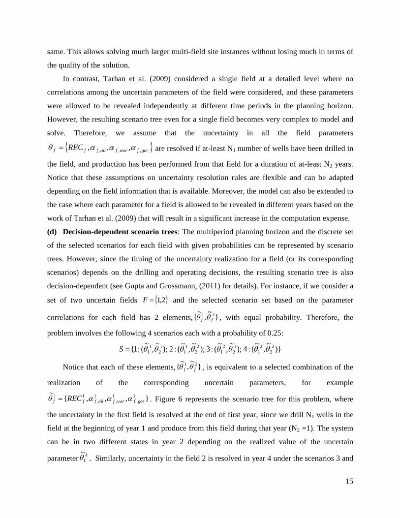
(d) Decision-dependent scenario trees: The multiperiod planning horizon and the discrete set

of the selected scenarios for each field with given probabilities can be represented by scenario

trees. However, since the timing of the uncertainty realization for a field (or its corresponding

scenarios) depends on the drilling and operating decisions, the resulting scenario tree is also

decision-dependent (see Gupta and Grossmann, (2011) for details). For instance, if we consider a

set of two uncertain fields { }2,1=F and the selected scenario set based on the parameter

correlations for each field has 2 elements, }~,~{ 21ff θθ , with equal probability. Therefore, the

problem involves the following 4 scenarios each with a probability of 0.25:

)}~,~(:4);~,~(:3);~,~(:2);~,~(:1{ 22

21

12

21

22

11

12

11 θθθθθθθθ=S

Notice that each of these elements, }~,~{ 21ff θθ , is equivalent to a selected combination of the

realization of the corresponding uncertain parameters, for example

},,,{~ 1,

1,

1,

11gorfworfoilfff REC αααθ = . Figure 6 represents the scenario tree for this problem, where

the uncertainty in the first field is resolved at the end of first year, since we drill N1 wells in the

field at the beginning of year 1 and produce from this field during that year (N2 =1). The system

can be in two different states in year 2 depending on the realized value of the uncertain

parameter k1

~θ . Similarly, uncertainty in the field 2 is resolved in year 4 under the scenarios 3 and

15

4 due to drilling and operating decisions, whereas it remains uncertain in the scenarios 1 and 2.

Therefore, the resulting scenario tree depends on the optimization decisions, which are not

known a priori, requiring modeling a superstructure of the all possible scenario trees that can

occur based on our decisions. Notice that the scenario-tree also allows considering the cases

where the number of wells drilled in a field is less than the one required for the uncertainty

resolution (i.e. N1 wells), and therefore, the corresponding scenarios remain indistinguishable.

Figure 6: Decision-dependent scenario tree for two fields

An alternate representation of the decision-dependent scenario-tree (Ruszczynski, 1997) is

used to model the problem as a multistage stochastic program in which the scenarios are treated

independently and related through the non-anticipativity constraints for states of different

scenarios that are identical (see Goel and Grossmann, 2006; and Gupta and Grossmann, 2011).

The problem is to determine the optimal investment and operating decisions to maximize

the contractor’s expected NPV for a given planning horizon considering the above production

sharing agreements and endogenous uncertainties. In particular, investment decisions in each

time period t and scenario s include FPSO facilities installation or expansion, and their respective

installation or expansion capacities for oil, liquid and gas, fields-FPSO connections, and the

number of wells that need to be drilled in each field f, given the restrictions on the total number

of wells that can be drilled in each time period t over all the given fields. Operating decisions

include the oil/gas production rates from each field f in each time period t under every scenario s.

Drill N1 wells in field 1 Year 1

Year 2

Year 5

Year 3

Year 4

11

~θ 2

1~θ

12

~θ 2

2~θ

Drill N1 wells in field 2

1,2 3 4

16

It is assumed that the installation and expansion decisions occur at the beginning of each

time period t, while operations take place throughout the time period. There is a lead time of l1

years for each FPSO facility initial installation, and a lead time of l2 years for the expansion of an

earlier installed FPSO facility. Once installed, we assume that the oil, liquid (oil and water) and

gas capacities of a FPSO facility can only be expanded once. These assumptions are made for the

sake of simplicity, and both the model and the solution approaches are flexible enough to

incorporate more complexities. In the next section, we propose a multistage stochastic

programming model for oilfield development planning with production sharing agreements and

decision-dependent uncertainty in the field parameters as described.

3. Multistage Stochastic Programming Model We present a general multistage stochastic programming model for offshore oilfield

development planning that considers the trade-offs involved between investment and operating

decisions, uncertainties in the field parameters and profit share with the government while

maximizing the overall expected NPV for the contractor. Notice that the model is intended to be

applied every year of the project in a rolling horizon manner, not just once for the entire planning

horizon. In this way, new data for the model is updated as it becomes available every year. The

constraints involved in the model are as follows:

(i) Objective Function: The objective function is to maximize the total expected NPV of the

contractor as in (1), which is the summation of the NPVs over all the scenarios having

probabilities sp . The NPV of a particular scenario s is the difference between discounted total

contractor’s gross revenue share and total cost over the planning horizon (2). The total

contractor’s share in a particular time period t and scenario s is the sum of the contractor’s share

over all the ring-fences (rf) as given in equation (3). Similarly, constraints (4) and (5) represent

the total capital and operating expenses for each scenario s in time period t.

ENPVMax (1)

∑∑ −−⋅=t

stott

stott

stottt

s

s OPERCAPTotalConShdispENPV )( ,,,

(2)

∑=rf

strf

stott TotalConShTotalConSh ,

,

st,∀ (3)

17

∑=rf

strf

stott CAPCAP ,

,

st,∀ (4)

∑=rf

strf

stott OPEROPER ,

,

st,∀ (5)

(ii) Cost Calculations: The total capital expenses in scenario s for a ring-fence rf contains two

components as given in equation (6). One is field specific (eq. 7) that accounts for the connection

costs between a field and a FPSO facility, and cost of drilling the wells for each of the field in

that ring-fence rf. The other cost component is FPSO specific (eq. 8) that includes the capital

expenses for the corresponding FPSO facilities. Eq. (9) calculates the total cost of an FPSO

facility in time period t for scenario s which is disaggregated in eq. (10) over various fields (and

therefore ring-fences as in (11)). The cost disaggregation is performed on the basis of the field

sizes to which the FPSO is connected (eq. (12)-(14)), where set Ffpso is the set of all the fields that

can be connected to FPSO facility fpso and the binary variable sonfpsofb ,

, represents the potential

connections. Notice that there is an uncertainty in the recoverable oil volume of the field ( sfREC )

used in eq. (14) that multiplies the binary variable sonfpsofb ,

, . To linearize the bilinear terms in eq.

(14), we use an exact linearization technique (Glover, 1975) by introducing the positive variables

( sfieldtfpsoff

sfieldtfpsoff ZDZD ,

,,,',

,,,' 1, ) and )1,( ,,,,s

tfpsofs

tfpsof ZDZD that results in the constraints (15)-(23).

strf

strf

strf CAPCAPCAP ,,, 21 +=

strf ,,∀ (6)

∑∑ ∑+=rf rfF fpso F

swelltf

welltf

stfpsoftfpsof

strf IFCbFCCAP ,

,,,,,,,1 strf ,,∀ (7)

∑=fpso

stfpsorf

strf DFPSOCCAP ,,,2

strf ,,∀ (8)

[ ])()( ,,

,,,

,,

,,,

,,,,

sgastfpso

sgastfpso

gastfpso

sliqtfpso

sliqtfpso

liqtfpso

sFPSOtfpso

FPSOtfpso

stfpso QEQIVCQEQIVCbFCFPSOC ++++=

strf ,,∀ (9)

∑=fpsoF

sfieldtfpsof

stfpso DFPSOCFPSOC ,

,,,

strf ,,∀ (10)

∑=rfF

sfieldtfpsof

stfpsorf DFPSOCDFPSOC ,

,,,,

stfpsorf ,,,∀ (11)

18

∑=t

stfpsof

sonfpsof bb ,,,

, sfpsof ,,∀ (12)

sonfpsof

sfieldtfpsof bMDFPSOC ,

,,

,, ⋅≤

stfpsof ,,,∀ (13)

stfpso

Ff

sf

sonfpsof

sf

sonfpsofsfield

tfpsof FPSOCRECb

RECbDFPSOC

fpso

,

''

,',

,,,

,, ⋅⋅

⋅=∑∈

stfpsof ,,,∀ (14)

sf

stfpsof

sf

Ff

sfieldtfpsoff RECZDRECZD

fpso

⋅=⋅∑∈

,,''

,,,',

stfpsof ,,,∀ (15)

sfieldtfpsof

sfieldtfpsoff

sfieldtfpsoff DFPSOCZDZD ,

,,,

,,',,

,,', 1 =+

sFftfpsof fpso ,',,, ∈∀ (16)

sonfpsof

sfieldtfpsoff bUZD ,

,',

,,,' ⋅≤

sFftfpsof fpso ,',,, ∈∀ (17)

)1(1 ,,'

,,,,'

sonfpsof

sfieldtfpsoff bUZD −⋅≤

sFftfpsof fpso ,',,, ∈∀ (18)

01,0 ,,,,'

,,,,' ≥≥ sfield

tfpsoffsfield

tfpsoff ZDZD

sFftfpsof fpso ,',,, ∈∀ (19)

stfpso

stfpsof

stfpsof FPSOCZDZD ,,,,, 1 =+

stfpsof ,,,∀ (20)

sonfpsof

stfpsof bUZD ,

,,, ⋅≤

stfpsof ,,,∀ (21)

)1(1 ,,,,

sonfpsof

stfpsof bUZD −⋅≤

stfpsof ,,,∀ (22)

01,0 ,,,, ≥≥ stfpsof

stfpsof ZDZD

stfpsof ,,,∀ (23)

The total operating expenses for scenario s in time period t for ring-fence rf , eq. (24), are

the operation costs corresponding to the total amount of liquid and gas produced.

[ ]stottrf

gastrf

stottrf

stottrf

liqtrft

strf gOCwxOCOPER ,

,,,

,,

,,, )( ++= δ

strf ,,∀ (24)

(iii) Total Contractor Share Calculations: The total contractor share in scenario s for ring-

fence rf in time period t, eq. (25), is the sum of contractor’s after-tax profit oil share for that ring-

fence and the cost oil that it keeps to recover the expenses. The contractor’s profit oil share after

tax in scenario s is the difference of the contractor’s profit oil share before tax and income tax

19

paid as in constraint (26). The tax paid by the contractor on its profit oil share depends on the

given tax rate ( taxtrff , ) as in constraint (27).

strf

saftertaxtrf

strf COConShTotalConSh ,

,,, +=

strf ,,∀

(25)

strf

sbeforetaxtrf

saftertaxtrf TaxConShConSh ,

,,

,, −=

strf ,,∀

(26)

sbeforetaxtrf

taxtrf

strf ConShfTax ,

,,, ⋅=

strf ,,∀ (27)

The contractor’s share before tax for scenario s in each time period t is some fraction of the

total profit oil during that period t for ring-fence rf. Note that we assume here that this profit oil

fraction, poirff , , is based on a decreasing sliding scale system that is linked to the cumulative

amount of oil produced strfxc , , where i is the index of the corresponding tier. Therefore, for

possible levels i (i.e. tiers) of cumulative amount of oil produced by the end of time period t in

scenario s, the corresponding contractor’s profit oil share can be calculated using disjunction (28)

where the boolean variable tirfZ ,, is true if the cumulative oil produced lies between the tier i

threshold. This disjunction (28) can further be rewritten as integer and mixed-integer linear

constraints (29)-(36) using the convex-hull formulation (Raman and Grossmann, 1994).

≤≤

⋅=∨

oilirf

strf

oilirf

strf

POirf

sbeforetaxtrf

stirf

i

UxcL

POfConSh

Z

,,,

,,,

,

,,

strf ,,∀ (28)

∑=i

sbeforetaxtirf

sbeforetaxtrf DConShConSh ,

,,,

,

strf ,,∀ (29)

∑=i

stirf

strf DPOPO ,,,

strf ,,∀ (30)

∑=i

stirf

strf Dxcxc ,,,

strf ,,∀ (31)

stirf

poirf

sbeforetaxtirf DPOfDConSh ,,,

,,, ⋅=

stirf ,,,∀

(32)

stirf

sbeforetaxtirf ZMDConSh ,,

,,,0 ⋅≤≤

stirf ,,,∀

(33)

20

stirf

stirf ZMDPO ,,,,0 ⋅≤≤

stirf ,,,∀

(34)

stirf

oilirf

stirf

stirf

oilirf ZUDxcZL ,,,,,,,, ⋅≤≤⋅

stirf ,,,∀ (35)

1,, =∑i

stirfZ

strf ,,∀

(36)

}1,0{,, ∈stirfZ

The cumulative amount of oil produced from a ring-fence rf by the end of time period t in

scenario s is calculated as the sum of the cumulative amount of oil produced by that time period

from all the fields associated to that ring-fence, eq. (37). Constraint (38) represents the total

profit oil in time period t for a ring-fence rf as the difference between gross revenue and the cost

oil for scenario s. The gross revenues (39) in each time period t for a ring-fence rf in scenario s,

are computed based on the total amount of oil produced and its selling price, where total oil flow

rate in time period t for ring-fence rf, is calculated as the sum of the oil production rates over all

the fields in that ring-fence, i.e. set Frf , in equation (40). For simplicity, we only consider the

revenue generated from the oil sales, which is much larger in general as compared to the revenue

from gas.

∑=rfF

sfieldtf

strf xcxc ,

,,

strf ,,∀ (37)

strf

strf

strf COREVPO ,,, −= strf ,,∀

(38)

stottrftt

strf xREV ,

,, αδ=

strf ,,∀ (39)

∑=rfF

stf

stottrf xx ,,

,

strf ,,∀ (40)

The cost oil in time period t for a ring-fence rf, constraint (41), is calculated as the

minimum of the cost recovery in that time period and maximum allowable cost oil (cost recovery

ceiling) in scenario s. Eq. (41) can further be rewritten as mixed-integer linear constraints (42)-

(47). Cost recovery in time period t for a ring-fence rf in scenario s, constraint (48), is the sum of

capital and operating costs in that period t and cost recovery carried forward from previous time

period t-1. Any unrecovered cost (that is carried forward to the next period) in time period t for a

21

ring-fence rf, is calculated as the difference between the cost recovery and cost oil in time period

t for a scenario s (eq. (49)).

),min( ,,,,s

trfCR

trfs

trfs

trf REVfCRCO ⋅=

strf ,,∀ (41)

)1( ,,,,

scotrf

strf

strf bMCRCO −+≤

strf ,,∀

(42)

)1( ,,,,

scotrf

strf

strf bMCRCO −−≥

strf ,,∀

(43)

scotrf

strf

CRtrf

strf bMREVfCO ,

,,,, ⋅+≤

strf ,,∀ (44)

scotrf

strf

CRtrf

strf bMREVfCO ,

,,,, ⋅−≥

strf ,,∀ (45)

strf

strf CRCO ,, ≤

strf ,,∀ (46)

strf

CRtrf

strf REVfCO ,,, ≤

strf ,,∀ (47)

strf

strf

strf

strf CRFOPERCAPCR 1,,,, −++= strf ,,∀

(48)

strf

strf

strf COCRCRF ,,, −= strf ,,∀

(49)

(iv) Tightening Constraints: The logic constraints (50) and (51) that define the tier sequencing

are included in the model to tighten its relaxation. These constraints can be expressed as integer

linear inequalities, (52) and (53), respectively, (Raman and Grossmann, 1991). In addition, the

valid inequalities (54), are also included to bound the cumulative contractor’s share in the

cumulative profit oil by the end of time period t, based on the sliding scale profit oil share and

cost oil that has been recovered (see Gupta and Grossmann, 2012b for details).

sirf

T

t

stirf ZZ ττ ,',,, ¬Λ⇒

= stiiirf ,,',, <∀ (50)

sirf

ts

tirf ZZ ττ ,',1,, ¬Λ⇒=

stiiirf ,,',, >∀ (51)

1,',,, ≤+ sirf

stirf ZZ τ

sTttiiirf ,,,',, ≤≤<∀ τ (52)

1,',,, ≤+ sirf

stirf ZZ τ

sttiiirf ,1,,',, ≤≤>∀ τ (53)

22

)/()()()/( ,,

'

1'',,1',',

,, ∑∑∑

≤

≤

=−

≤

⋅−−⋅−≤t

srf

POirf

ii

iirf

strf

POirf

POirf

t

sbeforetaxrf COfLxcffContsh end

τττ

τττ αα

stirf ,,,∀ (54)

(v) Reservoir Constraints: Constraints (55)-(58) predict the reservoir behavior for each field f

in each time period t for a scenario s. In particular, constraint (55) restricts the oil flow rate from

each well for a particular FPSO-field connection in time period t to be less than the deliverability

of that field per well in scenario s. Equation (56) represents the field deliverability per well in

scenario s at the beginning of time period t+1 for a particular FPSO-field connection as the cubic

equation in terms of the fractional oil recovered by the end of time period t from that field. In

particular, (56a) corresponds to the oil deliverability in time period 1, while (56b) corresponds to

the rest of the time periods in the planning horizon. Notice that the uncertainty in the oil

deliverability profile is characterized by the uncertain parameter soilα . Constraints (57) and (58)

represent the separable polynomials for the cumulative water and cumulative gas produced by

the end of time period t for a specific field-FPSO connection in scenario s, where swcα and s

gcα are

the respective uncertain parameters. The motivation for using polynomials for cumulative water

produced and cumulative gas produced as compared to WOR and GOR, is to avoid bilinear

terms in the formulation, and allow converting the resulting MINLP model into an MILP

formulation as explained in Gupta and Grossmann (2012a). swelldtfpsof

swelltfpsof Qx ,,

,,,

,, ≤

stfpsof ,,,∀ (55)

fpsofsoil

swelldfpsof dQ ,,1

,,1,, ⋅= α

sfpsof ,,∀ (56a)

])()([ ,,1,,,12

,,,13

,,,1,,

1,, fpsofs

tffpsofs

tffpsofs

tffpsofsoil

swelldtfpsof dfccfcbfcaQ +++⋅=+ α

sTtfpsof ,,, <∀ (56b)

])()()([ ,,,22

,,,23

,,,24

,,,2,

,,s

tffpsofs

tffpsofs

tffpsofs

tffpsofswc

swctfpsof fcdfccfcbfcaQ +++⋅= α

stfpsof ,,,∀ (57)

])()()([ ,,,32

,,,33

,,,34

,,,3,

,,s

tffpsofs

tffpsofs

tffpsofs

tffpsofsgc

sgctfpsof fcdfccfcbfcaQ +++⋅= α

stfpsof ,,,∀ (58)

23

Notice that variables swctfpsofQ ,

,, and sgctfpsofQ ,

,, will be non-zero in equations (57) and (58) if

stffc , is non-zero even though that particular field-FPSO connection is not present. Therefore,

additional constraints (59)-(66) need to be included to equate the actual cumulative water

produced ( stfpsofwc ,, ) and cumulative gas produced ( s

tfpsofgc ,, ) for a field-FPSO connection by

the end of time period t to the corresponding dummy variables swctfpsofQ ,

,, and sgctfpsofQ ,

,, only if that

field-FPSO connection is present in time period t, else it is zero.

∑=

−+≤t

sfpsof

swcfpsof

swctfpsof

stfpsof bMQwc

1,,

,,

,,,,, )1(

ττ

stfpsof ,,,∀ (59)

∑=

−−≥t

sfpsof

swcfpsof

swctfpsof

stfpsof bMQwc

1,,

,,

,,,,, )1(

ττ

stfpsof ,,,∀ (60)

∑=

≤t

sfpsof

swcfpsof

stfpsof bMwc

1,,

,,,,

ττ

stfpsof ,,,∀ (61)

∑=

−≥t

sfpsof

swcfpsof

stfpsof bMwc

1,,

,,,,

ττ

stfpsof ,,,∀ (62)

∑=

−+≤t

sfpsof

sgcfpsof

sgctfpsof

stfpsof bMQgc

1,,

,,

,,,,, )1(

ττ

stfpsof ,,,∀ (63)

∑=

−−≥t

sfpsof

sgcfpsof

sgctfpsof

stfpsof bMQgc

1,,

,,

,,,,, )1(

ττ

stfpsof ,,,∀ (64)

∑=

≤t

sfpsof

sgcfpsof

stfpsof bMgc

1,,

,,,,

ττ

stfpsof ,,,∀ (65)

∑=

−≥t

sfpsof

sgcfpsof

stfpsof bMgc

1,,

,,,,

ττ

stfpsof ,,,∀ (66)

Eq. (67) and (68) compute the water and gas flow rates in time period t from a field to

FPSO facility in scenario s as the difference of cumulative amounts produced by the end of

current time period t and previous time period t-1, divided by the time duration of that period.

ts

tfpsofs

tfpsofs

tfpsof wcwcw δ/)( 1,,,,,, −−=

stfpsof ,,,∀ (67)

ts

tfpsofs

tfpsofs

tfpsof gcgcg δ/)( 1,,,,,, −−=

stfpsof ,,,∀ (68)

24

(vi) Field-FPSO flow constraints: The total oil flow rate in (69) from each field f in time period

t for a scenario s is the sum of the oil flow rates that are directed to FPSO facilities in that time

period t, whereas oil that is directed to a particular FPSO facility from a field f in scenario s is

calculated as the multiplication of the oil flow rate per well and number of wells available for

production in that field (eq. (70)). Eq. (71) computes the cumulative amount of oil produced

from field f by the end of time period t in scenario s, while (72) represents the fractional oil

recovery by the end of time period t. The cumulative oil produced in scenario s is also restricted

in (73) by the recoverable amount of oil from the field. Eqs. (74)-(76) compute the total oil,

water and gas flow rates into each FPSO facility, respectively, in time period t from all the given

fields in each scenario s. The total oil, water and gas flowrates in each time period t for scenario

s are calculated as the sum of the production rate of these components over all the FPSO

facilities in equations (77)-(79), respectively.

∑=fpso

stfpsof

stf xx ,,,

stf ,,∀ (69)

swelltfpsof

swelltf

stfpsof xNx ,

,,,

,,, ⋅=

stfpsof ,,,∀ (70)

)(1

,, ττ

τδ∑=

=t

sf

stf xxc

stf ,,∀ (71)

sf

stfs

tf RECxc

fc ,, =

stf ,,∀ (72)

sf

stf RECxc ≤,

stf ,,∀ (73)

∑=f

stfpsof

stfpso xx ,,,

stfpso ,,∀ (74)

∑=f

stfpsof

stfpso ww ,,,

stfpso ,,∀ (75)

25

∑=f

stfpsof

stfpso gg ,,,

stfpso ,,∀ (76)

∑=fpso

stfpso

stott xx ,

,

st,∀ (77)

∑=fpso

stfpso

stott ww ,

,

st,∀ (78)

∑=fpso

stfpso

stott gg ,

,

st,∀ (79)

(vii) FPSO Capacity Constraints: Eqs. (80)-(82) restrict the total oil, liquid and gas flow rates

into each FPSO facility to be less than its corresponding capacity in each time period t,

respectively. These three different kinds of capacities of a FPSO facility in time period t are

computed by equalities (83)-(85) as the sum of the corresponding capacity at the end of previous

time period t-1, installation capacity at the beginning of time period t-l1 and expansion capacity

at the beginning of time period t-l2, where l1 and l2 are the lead times for FPSO installation and

expansions, respectively.

soiltfpso

stfpso Qx ,

,, ≤ stfpso ,,∀ (80)

sliqtfpso

stfpso

stfpso Qwx ,

,,, ≤+

stfpso ,,∀ (81)

sgastfpso

stfpso Qg ,

,, ≤ stfpso ,,∀ (82)

soilltfpso

soilltfpso

soiltfpso

soiltfpso QEQIQQ ,

,,

,,

1,,

, 21 −−− ++=

stfpso ,,∀ (83)

sliqltfpso

sliqltfpso

sliqtfpso

sliqtfpso QEQIQQ ,

,,

,,

1,,

, 21 −−− ++=

stfpso ,,∀ (84)

sgasltfpso

sgasltfpso

sgastfpso

sgastfpso QEQIQQ ,

,,,

,1,

,, 21 −−− ++=

stfpso ,,∀ (85)

26

(viii) Logic Constraints: Inequalities (86) and (87) restrict the installation and expansion of a

FPSO facility to take place only once, respectively, while inequality (88) states that the

connection between a FPSO facility and a field can be installed only once during the whole

planning horizon. Inequality (89) ensures that a field can be connected to at most one FPSO

facility in each time period t, while (90) states that at most one FPSO-field connection is possible

for a field f during the entire planning horizon under each scenario s. Constraints (91) and (92)

state that the expansion in the capacity of a FPSO facility and the connection between a field and

a FPSO facility, respectively, in time period t can occur only if that FPSO facility has already

been installed by that time period.

1, ≤∑∈Tt

stfpsob

sfpso,∀ (86)

1,, ≤∑

∈Tt

sextfpsob

sfpso,∀ (87)

1,,, ≤∑

∈Tt

sctfpsofb

sfpsof ,,∀ (88)

1,,, ≤∑

fpso

sctfpsofb

stf ,,∀ (89)

1,,, ≤∑∑

∈Tt fpso

sctfpsofb

sf ,∀

(90)

∑=

≤t

sfpso

sextfpso bb

1,

,,

ττ

stfpso ,,∀ (91)

∑=

≤t

sfpso

sctfpsof bb

1,

,,,

ττ

stfpsof ,,,∀ (92)

(ix) Upper bounding constraints: Inequality (93) states that the oil flow rate per well from a

field f to a FPSO facility in time period t will be zero if that FPSO-field connection is not

available in that time period in a scenario s. Constraints (94)-(99) are the upper-bounding

constraints on the installation and expansion capacities for FPSO facilities in time period t for

each scenario s. The additional upper bounds on the oil, liquid and gas expansion capacities of

FPSO facilities, (100)-(102), follow from the fact that these expansion capacities should be less

than a certain fraction (µ) of the initial built capacities, respectively.

27

∑=

≤t

scfpsof

oilwellfpsof

swelltfpsof bUx

1

,,,

,,

,,,

ττ

stfpsof ,,,∀ (93)

stfpso

oilfpso

soiltfpso bUQI ,

,, ≤

stfpso ,,∀ (94) s

tfpsoliqfpso

sliqtfpso bUQI ,

,, ≤

stfpso ,,∀ (95) s

tfpsogasfpso

sgastfpso bUQI ,

,, ≤

stfpso ,,∀ (96) sex

tfpsooilfpso

soiltfpso bUQE ,

,,

, ≤ stfpso ,,∀ (97)

sextfpso

liqfpso

sliqtfpso bUQE ,

,,

, ≤ stfpso ,,∀ (98)

sextfpso

gasfpso

sgastfpso bUQE ,

,,, ≤

stfpso ,,∀ (99) soil

tfpsosoil

tfpso QQE ,1,

,, −≤ µ

stfpso ,,∀ (100)

sliqtfpso

sliqtfpso QQE ,

1,,

, −≤ µ

stfpso ,,∀ (101) sgastfpso

sgastfpso QQE ,

1,,, −≤ µ

stfpso ,,∀ (102)

(x) Well drilling limitations: The number of wells available for production from a field in

scenario s is calculated from (103) as the sum of the wells available at the end of previous time

period and the number of wells drilled at the beginning of time period t. The maximum number

of wells that can be drilled over all the fields during each time period t and in each field f during

complete planning horizon are restricted by the respective upper bounds in (104) and (105). swell

tfswell

tfswell

tf INN ,,

,1,

,, += −

stf ,,∀ (103)

wellt

f

swelltf UII ≤∑ ,

, st,∀

(104)

wellf

swelltf UNN ≤,

, stf ,,∀ (105)

(xi) Initial Non-anticipativity Constraints: In addition to the above constraints (1)-(105) that

are equivalent to the constraints for the deterministic model with fiscal rules for each scenario s

as in Gupta and Grossmann (2012b), we need the initial non-anticipativity constraints, eqs.

(106)-(115), for time periods TTI ⊂ where the set IT may include only first or few initial time

periods. These constraints ensure that we make the same decisions (FPSO installations,

expansions and their oil, liquid, gas capacities; well drilling schedule and field-FPSO

28

connections) in scenarios s and s’ until uncertainty in the any of the parameters cannot be

revealed.

IsFPSO

tfpsosFPSO

tfpso Ttssfpsobb ∈∀= ,',,',,

,,

(106)

Isex

tfpsosex

tfpso Ttssfpsobb ∈∀= ,',,',,

,,

(107)

Is

tfpsofs

tfpsof Ttssfpsofbb ∈∀= ,',,,',,,,

(108)

Iswell

tfswell

tf TtssfII ∈∀= ,',,',,

,,

(109)

Isoil

tfpsosoil

tfpso TtssfpsoQIQI ∈∀= ,',,',,

,,

(110)

Isliq

tfpsosliq

tfpso TtssfpsoQIQI ∈∀= ,',,',,

,,

(111)

Isgastfpso

sgastfpso TtssfpsoQIQI ∈∀= ,',,',

,,,

(112)

Isoil

tfpsosoil

tfpso TtssfpsoQEQE ∈∀= ,',,',,

,,

(113)

Isliq

tfpsosliq

tfpso TtssfpsoQEQE ∈∀= ,',,',,

,,

(114)

Isgastfpso

sgastfpso TtssfpsoQEQE ∈∀= ,',,',

,,,

(115)

(xii) Conditional Non-anticipativity Constraints: To determine the scenario pairs (s, s’) that

are indistinguishable at the beginning of time period t, we consider the uncertainty resolution

rule as explained in section 2.3. In particular, we assume that the uncertainty in all the

parameters of a field is revealed if we drill at-least N1 number of wells in the field, and produce

from that field for at-least N2 number of years. Therefore, eq. (116) is used relate the number of

wells in the field to the binary variable stfw ,1, such that the variable s

tfw ,1, is true if and only if the

number of wells drilled in the field are less than N1. Similarly, the production from the field f has

been made for less than N2 years, if and only if stfw ,2, is true as represented in eqs. (117)-(118).

The logic constraint (119) sets the value of the binary variable stfw ,3, to be true if and only if

either of stfw ,1, or s

tfw ,2, are true, i.e. uncertainty in the field f has not been revealed in scenario s at

the beginning of time period t.

)1( 1,1,

,1, −≤⇔ − NNw swell

tfstf

stf ,,∀ (116)

29

)1( 2

1

1

,,

,2, −≤⇔ ∑

−

=

Nbwt

sprodf

stf

ττ

stf ,,∀ (117)

)( ,,

, ε≥⇔ stf

sprodtf xb

stf ,,∀

(118)

stf

stf

stf www ,2

,,1,

,3, ∨⇔

stf ,,∀ (119)

Based on the above value of the variable stfw ,3, , equation (120) determines the value of the

boolean variable ',sstZ . In particular, two scenarios (s, s’) will be indistinguishable at the

beginning of time period t if and only if for each field f that distinguishes those scenarios (i.e.

)',( ssDf ∈ ), stfw ,3, is true. Therefore, eqs. (116)-(120) can be used to determine the

indistinguishable scenarios at the beginning of time period t based on the decisions that have

been implemented before that time period. Notice that as a special case, where either well

drilling or production from the field is sufficient to observe the uncertainty, then one only needs

to consider eq. (116) or eqs. (117)-(118), respectively, and eq. (120) without introducing the

additional variable stfw ,3, .

stfssDf

sst wZ ,3

,)',(

',

∈∧⇔

tss ,',∀

(120)

The conditional non-anticipativity constraints in disjunction (121) equate the decisions in

scenarios s and s’ for the later time periods TTC ⊂ , if these scenarios are indistinguishable at

the beginning of time period t, i.e. for which ',sstZ is true calculated in eq. (120).

30

[ ] Css

t

sgastfpso

sgastfpso

sliqtfpso

sliqtfpso

soiltfpso

soiltfpso

sgastfpso

sgastfpso

sliqtfpso

sliqtfpso

soiltfpso

soiltfpso

swelltf

swelltf

stfpsof

stfpsof

sextfpso

sextfpso

sFPSOtfpso

sFPSOtfpso

sst

TtssZ

fpsoQEQE

fpsoQEQE

fpsoQEQE

fpsoQIQI

fpsoQIQI

fpsoQIQI

fII

fpsofbb

fpsobb

fpsobb

Z

∈∀¬∨

∀=

∀=

∀=

∀=

∀=

∀=

∀=

∀=

∀=

∀=

,',

,

'.

',,

,,

',,

,,

',,

,,

',,

,,

',,

,,

',,

,,

',,

,,

',,,,

',,

,,

',,

,,

',

(121)

The multistage stochastic mixed-integer nonlinear disjunctive programming model (MSSP-

ND) for offshore oilfield investment and operations planning involves constraints (1)-(13), (15)-

(27), (29)-(40), (42)-(49), (52)-(121) that consider endogenous uncertainty in the field

parameters and sliding scale production sharing agreements with ringfencing provisions. In

particular, constraints (56b)- (58) and (70) are nonlinear and non-convex constraints in the

model. These constraints can be linearized using exact linearization and piecewise linear

approximation techniques described in Gupta and Grossmann (2012a) to convert the nonlinear

model (MSSP-ND) to a linear one (MSSP-LD). Notice that the resulting model will be an

extension of the deterministic MILP fiscal model (Model 3F) in Gupta and Grossmann (2012b)

to the stochastic case using the modeling framework presented in Gupta and Grossmann (2011).

4. Compact representation of the Multistage Stochastic Model The proposed multistage stochastic mixed-integer linear disjunctive programming model

(MSSP-LD) in the previous section can be represented in the following compact form, where all

the variables in the detailed model, integer and continuous, are aggregated into the variables stx :

31

(MD) ∑ ∑∈ ∈

=Ss Tt

stt

s xcpzmax (122)

staxAts st

t

ss ,.. ∀≤∑≤τ

ττ (123)

SssTtxx Ist

st ∈∀∈∀= ',,'

(124)

SssTtxxxFZ Cst

sssst ∈∀∈∀⇔ − ',,)....,( 121

', (125)

SssTtZxx

ZC

sst

st

st

sst

∈∀∈∀

¬∨

=',,

',

'

',

(126)

',, JjstIxsjt ∈∀∀∈ (127)

'\,, JJjstRxsjt ∈∀∀∈ (128)

The objective function (122) in the above model (MD) maximizes the expectation of an

economic criterion over the set of scenarios Ss∈ , and over a set of time periods Tt∈ , which is

equivalent to eq. (1). For a particular scenario s, inequality (123) represents constraints that

govern decisions stx in time period t and link decisions across time periods. These individual

scenario constraints correspond to the eqs. (2)-(13), (15)-(27), (29)-(40), (42)-(49) and (52)-

(105), where the nonlinear and non-convex constraints (56b)- (58) and (70) have been linearized

using exact linearization and piecewise linear approximation techniques described in Gupta and

Grossmann (2012a).

Non-anticipativity (NA) constraints for initial time periods TTI ⊂ are given by equations

(124) for each scenario pair (s,s’) to ensure the same decisions in all the scenarios, which are the

compact representation for constraints (106)-(115). The conditional NA constraints are written

for the later time periods TTC ⊂ in terms of logic propositions (125) and disjunctions (126).

Notice that the set of initial time periods IT may include first few years of the planning horizon

until uncertainty cannot be revealed, while CT represents the rest of the time periods in the

planning horizon. The function )....,( 121st

ss xxxF − in eq. (125) is an uncertainty resolution rule for a

given pair of scenarios s and s’ that determines the value of the corresponding boolean variable ',ss

tZ based on the decisions that have been implemented so far as shown in eqs. (116)-(120). The

32

variable ',sstZ is further used in disjunction (126) to ensure the same decisions in scenarios s and

s’ if these are still indistinguishable in time period t, which is similar to the disjunctions (121).

Equations (127)-(128) define the domain of the discrete and continuous variables in the model.

Notice that the model with a reduced number of scenario pairs (s,s’) that are sufficient to

represent the non-anticipativity constraints can be obtained from model (MD) after applying the

three properties presented in Gupta and Grossmann (2011). These properties are defined on the

basis of symmetry, adjacency and transitivity relationship among the scenarios. The reduced

model (MDR) can be formulated from (MD) as follows, where 3P is the set of minimum number

of scenario pairs that are required to represent non-anticipativity in each time period t,

(MDR) ∑ ∑∈ ∈

=Ss Tt

stt

s xcpzmax (122)

staxAts st

t

ss ,.. ∀≤∑≤τ

ττ (123)

3' )',(, PssTtxx I

st

st ∈∀∈∀= (129)

3121', )',(,)....,( PssTtxxxFZ C

st

sssst ∈∀∈∀⇔ − (130)

3

',

'

',

)',(, PssTtZxx

ZC

sst

st

st

sst

∈∀∈∀

¬∨

= 131)

',, JjstIxsjt ∈∀∀∈ (127)

'\,, JJjstRxsjt ∈∀∀∈ (128)

The mixed-integer linear disjunctive model (MDR) can be further converted to a mixed-

integer linear programming model (MLR). First, the logic constraints (130) are re-written as the

mixed-integer linear constraints eq. (132) based on the uncertainty resolution rule where ',sstz is a

binary variable that takes a value of 1 if scenario pair (s,s’) is indistinguishable in time period t,

else it is zero. The disjunction (131) can then be converted to mixed-integer linear constraints

(133) and (134) using the big-M formulation. The resulting mixed-integer linear model (MLR)

includes constraints (122), (123), (129), (132), (133), (134), (127) and (128).

3', )',(, PssTtdzCxB C

st

sst

st

st

st ∈∀∈∀≤+ (132)

33

3'', )',(,)1( PssTtxxzM C

st

st

sst ∈∀∈∀−≤−− (133)

3'', )',(,)1( PssTtxxzM C

st

st

sst ∈∀∈∀−≥− (134)

Figure 7: Structure of a typical Multistage Stochastic Program with Endogenous uncertainties

Figure 7 represents the block angular structure of model (MLR), where we can observe

that the initial (eq. (129)) and conditional (eqs. (132), (133) and (134)) non-anticipativity

constraints link the scenario subproblems. Therefore, these are the complicating constraints in

the model. However, this structure allows decomposing the fullspace problem into smaller

subproblems by relaxing the linking constraints as in Gupta and Grossmann (2011). It should be

noted that the NACs (especially conditional NACs) represent a large fraction of the total

constraints in the model. For clarity, we use this compact representation (MLR) in the next

section to describe the solution approach instead of the detailed model (MSSP-LD) presented in

the previous section.

5. Solution Approach The reduced model (MLR) is composed of scenario subproblems connected through the initial

(eq. (129)) and conditional (eqs. (132), (133) and (134)) non-anticipativity (NA) constraints. If

these NA constraints are either relaxed or dualized using Lagrangean decomposition, then the

problem decomposes into smaller subproblems that can be solved independently for each

scenario within an iterative scheme for the multipliers as described in Carøe and Schultz (1999)

and in Gupta and Grossmann (2011). In this way, we can effectively decompose and solve the

Scenario Constraints

Initial NACs

Conditional NACs

34

large-scale oilfield development planning instances. The Lagrangean decomposition algorithm of

Figure 8 for MSSP with endogenous uncertainties as proposed in Gupta and Grossmann (2011)

involves obtaining the upper bound (UB) by solving the Lagrangean problem (L1-MLR) with

fixed multipliers ',sstλ . The Lagrangean problem (L1-MLR) is formulated from the mixed-integer

linear reduced model (MLR) by relaxing all the conditional NA constraints (132), (133) and

(134), and dualizing all the initial NA constraints (129) as penalty terms in the objective

function. This gives rise to the subproblems for each scenario Ss∈ , (L1-MLRs) that can be

solved independently in parallel.

(L1-MLR) ∑ ∑∑ ∑∈ ∈∈ ∈

−+1 3)',(

'', )(maxTt Pss

st

st

sst

Ss Tt

stt

s xxxcp λ (135)

staxAts st

t

ss ,.. ∀≤∑≤τ

ττ (136)

',,}1,0{ Jjstxsjt ∈∀∀∈ (137)

'\,, JJjstRxsjt ∈∀∀∈ (138)

(L1-MLRs) ∑ ∑ ∑∑∈

<∈

>∈∈

−+1 3 3

')',(

'),'(

,'', )(maxTt

ssPss

ssPss

sst

sst

st

Tt

stt

s xxcp λλ (139)

taxAts st

t

ss ∀≤∑≤τ

ττ.. (140)

',}1,0{ Jjtxsjt ∈∀∀∈ (141)

'\, JJjtRxsjt ∈∀∀∈ (142)

The lower bound (LB) or feasible solution is generated by using a heuristic based on the

solution of the Lagrangean problem (L1-MLR). In this heuristic, we fix the decisions obtained

from the above problem (L1-MLR) in the reduced problem (MLR) such that there is no violation

of NA constraints and solve it to obtain the lower bound. The sub-gradient method by Fisher

(1985) is used during each iteration to update the Lagrangean multipliers. The algorithm, which

is shown in Figure 5, stops when either a maximum iteration/time limit is reached, or the

difference between the lower and upper bounds, LB and UB, is less than a pre-specified

tolerance.

35

Notice that the extended form of this method relying on duality based branch and bound

search, has also been proposed in Goel and Grossmann (2006), Tarhan et al. (2009), and Tarhan

et al. (2011) to close the gap between the upper and the lower bounds. Moreover, a new

Lagrangean decomposition algorithm is proposed in the next Gupta and Grossmann (2013) to

further improve the quality of the dual bound at the root node.

6. Numerical Results In this section, we present computational results for the offshore oilfield development planning

examples under endogenous uncertainty in the field parameters, which resolves as a function of

investment and operating decisions as described before. Moreover, we consider a case where

progressive production sharing agreements are also present. The multistage stochastic MILP

model (MLR) presented in section 4 is considered that maximizes the expected NPV value over

the given planning horizon. The model is implemented in GAMS 23.6.3 and run on an Intel Core

i7, 4GB RAM machine using CPLEX 12.2 solver for all the instances.

6.2.1 3 Oilfield Planning Example

Case (i): Uncertainty in the field size only (4 scenarios)

Initial Multipliers (λ0) and iteration no. k = 0

LB = -∞ UB = ∞

Yes

Solve Lagrangean subproblem with fixed multipliers to get UB

Gap < ε or k > kmax

Stop

Find LB (Feasible Solution) by using a heuristic

No

Update Lagrangean multipliers using Sub-gradient method

Figure 5: Lagrangean Decomposition algorithm

36

In this instance, we consider 3 oilfields and 3 potential FPSO’s that can be installed. There are a

total of 9 possible connections among field-FPSO (Figure 9), and 30 wells can be drilled in the

fields over the planning horizon of 10 years. Field 3 has a recoverable oil volume (field size) of

500 MMbbls. However, there is uncertainty in the size of fields 1 and 2, where each one has two

possible realizations (low, high) with equal probability. Therefore, there are a total of 4 scenarios

each with a probability of 0.25 (see Table 1). Notice that for simplicity we only consider the

cases with same probabilities for all the scenarios throughout this paper. In our future paper, if it

would be possible, we will include more realistic probability values for the examples.

Figure 9: 3 oilfield planning example

Table 1: 3 oilfield planning example, case (i)

Scenarios s1 s2 s3 s4

Field 1 Size (MMbbls) 57 403 57 403

Field 2 Size (MMbbls) 80 80 560 560

Scenario Probability 0.25 0.25 0.25 0.25

It is assumed that the uncertainty in field 1 size is revealed after drilling 3 wells (N1= 3) in

the field and producing for 1 year (N2= 1) from it. Whereas, field 2 needs at-least 4 wells to be

drilled (N1= 4) and one year of production (N2= 1) for this purpose. The problem is to determine

the optimum investment (FPSO installations and expansions, field-FPSO connections and well

drilling) and operating decisions (oil production rate) with an objective to maximize the total

expected NPV (ENPV) over the planning horizon.

FPSO 1 FPSO 3

Field 1

Field 3

Field 2

Total Oil/Gas Production

FPSO 2

37

Table 2: Model statistics for the 3 oilfield example, case (i)

1 2 3 4

Figure 10: Optimal solution for 3 oilfield example, case (i)

The optimal ENPV for the problem is $11.50 billion when the reduced model (MLR) is

solved in fullspace using CPLEX 12.2 solver requiring 1184s. Table 2 presents the model

statistics for this instance. The solution suggests installing only FPSO 3 in the first year (see

Figure 10) with a capacity of 500 kstb/d and 333.5 MMSCF/d for liquid and gas, respectively.

The facility is available to produce at the beginning of year 4 due to a lead time of three years.

Then, we drill 3, 5 and 12 wells in fields 1,2 and 3, respectively, given the drilling-rig limitation

of a total 20 wells in a year. Since, fields 1 and 2 have uncertainties, based on the realization of

the uncertainty in their field sizes, more wells are drilled in these fields in the future for the

favorable scenarios compared to the unfavorable outcomes, whereas no more wells are drilled in

field 3. In particular, the favorable scenarios for field 1 are scenarios 2 and 4, where a total of 7

wells are drilled in the field. On the other hand, field 2 has favorable scenarios 3 and 4, where a

L,L H,H

drill (3,5,12)

drill (1,0) (4,0) (0,6) (4,6)

H,L L,HUncertainty Revealed

Year 1

Year 4

Year 5

Year 6

Year 7

Year 8

Year 9

Year 10

Build FPSO 3 (500, 333.5)

drill (0,2) (0,4) (3,0)

Problem Type

Number of

Constraints

Continuous

Variables

Discrete

Variables

SOS1

Variables

Reduced Model (MLR) 16,473 9,717 876 240 Individual Scenario 3,580 2,390 179 60

38

total of 11 wells are drilled in the field. Due to the different drilling and production decisions in

different scenarios based on the uncertainty realizations, the capacity of FPSO3 is expanded in

year 5 for scenarios 2, 3 and 4, whereas no expansion is made in the FPSO3 capacity in scenario

1. We can observe that the optimal scenario-tree is decision-dependent which is not known a-

priori (Figure 10).

Figure 11: Lagrangean decomposition results for 3 oilfield example, case (i)

The multistage stochastic model (MLR) is also solved using the Lagrangean decomposition

algorithm presented in the previous section that relies on dualizing the initial NACs and

removing the conditional NACs. Figure 11 demonstrates the progress of the bounds obtained at

the root node using this decomposition approach. A termination criterion of either 1% gap or 20

sub-gradient iterations is used. We can observe that the problem can be solved in ~1% optimality

tolerance in only 466s for the sequential implementation compared to the fullspace model that

takes 1184s. Moreover, the parallel implementation of the Lagrangean decomposition algorithm

in GAMS with 8 processors only takes 259s. Therefore, the proposed strategy reduces the

solution time for this 4 scenario instance by more than 75% compared to the fullspace model. It

is also important to note that the reformulation of the MINLP model (Model 2) to MILP

approximation (Model 3) in Gupta and Grossmann (2012a) allows us to use this decomposition

strategy with valid upper and lower bounds on the objective function value, without solving the

11.45

11.50

11.55

11.60

11.65

11.70

11.75

11.80

11.85

0 2 4 6 8 10 12 14 16 18 20

ENPV

(bill

ion

dolla

rs)

Iterations

LB

UB

39

non-convex MINLP model to global optimality which is quite expensive. Notice that the solution

of the expected value problem considering the mean value of the field sizes is $11.28 billion.

Therefore, the value of the stochastic solution for this case is $220 million or ~2%.

Case (ii): Uncertainty in the field size, oil deliverability, WOR and GOR (4 scenarios)

In this case, we consider uncertainty in the field size, oil deliverability, water-oil ratio (WOR)

and gas-oil-ratio (GOR) for oilfields 1 and 2. Notice that oil deliverability, WOR and GOR are

represented by the univariate polynomials in terms of the fractional oil recovery as shown in

equations (143)-(145), respectively.

)( fcgQ od ⋅=α (143)

)( fcgwor w ⋅=α (144)

)( fcggor g ⋅=α (145)

The uncertainty in oil deliverability, WOR and GOR is characterized by the uncertainty in

corresponding parameters oα , wα and gα . We assume that the uncertain parameters for a field

are correlated, and that uncertainty in these parameters is resolved at the same time as explained

earlier. This allows us to reduce a large number of scenarios in the problem. The two possible

combinations of these parameters for each field results in a total of 4 scenarios each with a

probability of 0.25 as can be seen in Table 3. The data for the rest of the problem are as in case

(i) presented above.

Table 4 summarizes the computational results for this case, and we can observe the similar

trends as in the previous case. In particular, the fullspace multistage stochastic model using

CPLEX 12.2 takes >10,000s to solve the problem to optimality and it yields an expected NPV

value of $11.95 billion. The sequential and parallel implementations (8 processors) of the

proposed Lagrangean decomposition approach provide a solution of $11.94 billion with more

than an order of magnitude reduction in solution times. To further reduce the gap between the

upper and the lower bounds, the algorithm can be extended to the duality based branch and

bound search procedure as proposed in Goel and Grossmann (2006). In addition, an improved

Lagrangean decomposition approach that yields a tighter dual bound at the root node is also

presented in Gupta and Grossmann (2013).

40

Table 3: 3 oilfield planning example, case (ii)

Scenarios s1 s2 s3 s4

Field 1

Size (MMbbls) 57 403 57 403

oα 0.75 1.25 0.75 1.25

wα 0.75 1.25 0.75 1.25

gα 0.75 1.25 0.75 1.25

Field 2

Size (MMbbls) 80 80 560 560

oα 0.75 0.75 1.25 1.25

wα 0.75 0.75 1.25 1.25

gα 0.75 0.75 1.25 1.25

Scenario Probability 0.25 0.25 0.25 0.25

Table 4: Computational results for 3 oilfield example, case (ii)

Fullspace Lagrangean Decomposition

Sequential Parallel

UB ($109) 11.95 12.14 12.14

LB ($109) 11.95 11.94 11.94

Solution Time (s) 10390 438 257

% Gap 0% 1.66% 1.66%

Subgradient iterations - 20 20

Case (iii): Uncertainty in the field size and progressive production sharing agreements

We also extend the 3 oilfield example to the case where we include the progressive production

sharing agreements and a planning horizon of 15 years. Table 5 represents the sliding scale profit

share of the contactor involving 3 tiers that are defined on the basis of the cumulative oil

production. The cost recovery ceiling of 50% of the gross revenue every year and an income tax

rate of 30% is also considered. There is uncertainty in the field sizes (field 1 and 2) with a total

of 4 scenarios as described in Table 1.

The multistage stochastic model becomes very difficult to solve for this instance in

fullspace due to the complexities introduced in the model by the non-anticipativity constraints,

and the disjunction for representing the sliding scale fiscal rules. In particular, the best solution

obtained after 10 hours in fullspace using CPLEX 12.2 solver is $2.97 billion with more than

41

21% of optimality gap (see Table 6). On the other hand, the proposed Lagrangean decomposition

can solve this problem in approximately 2 hrs for the sequential implementation of the scenario

subproblem solutions, and in about 1 hr for the parallel implementation (8 processors). Both the

cases yield a higher ENPV $3.04 billion within a 0.7% of optimality tolerance. Therefore, this

example illustrates the importance of the decomposition algorithm, and its parallel

implementation as more complexities are added to the problem, such as the progressive fiscal

rules.

Table 5: Sliding scale contractor’s profit oil share for the 3 oilfield example, case (iii) Tiers Cumulative Oil Produced Contractor’s Share in Profit Oil

Tier 1 0-350 MMbbl 50%

Tier 2 350-700 MMbbl 40%

Tier 3 >700 MMbbl 20%

Table 6: Computational results for 3 oilfield example, case (iii)

Fullspace Model Lagrangean Decomposition

#

Constraints

#

Dis. Var.

#

Cont. Var.

ENPV

($109)

Time

(s)

ENPV

($109)

Sequential

Time (s)

Parallel

Time (s)

27,113 1,536 15,857 $2.97

(>21%)

>36,000 $3.04

(0.7%)

8,990 4,002

6.2 5 Oilfield Planning Example

Case (i): Uncertainty in the field size only (8 scenarios)

This is a larger example for oilfield planning problem under uncertainty than the previous

one, where we consider 5 oilfields that can be connected to 3 FPSOs with 13 possible

connections (Figure 12). A total of 51 wells can be drilled in the fields over the planning horizon

of 20 years. There is uncertainty in the size of fields 1, 3 and 5, where each one has two possible

realizations (low, high) with equal probability. Therefore, there are a total of 8 scenarios each

with a probability of 0.125 (see Table 7). Fields 2 and 4 have known recoverable oil volumes of

200 and 400 MMbbls, respectively.

It is assumed that the uncertainty in field 1 size is revealed after drilling 3 wells (N1= 3) in

the field and producing for 1 year (N2= 1) from it. Fields 3 and 5 need at-least 4 wells to be

42

drilled (N1= 4) and one year of production (N2= 1) for this purpose. The problem is to determine

the optimum investment (FPSO installations and expansions, field-FPSO connections and well

drilling) and operating decisions (oil production rate) with an objective to maximize the total

expected NPV (ENPV) over the planning horizon.

Figure 12: 5 oilfield planning example

Table 7: 5 oilfield planning example, case (i)

Scenarios s1 s2 s3 s4 s5 s6 s7 s8

Field 1 Size

(MMbbls)

57 403 57 403 57 403 57 403

Field 3 Size

(MMbbls)

80 80 560 560 80 80 560 560

Field 5 Size

(MMbbls)

125 125 125 125 875 875 875 875

Scenario Probability 0.125 0.125 0.125 0.125 0.125 0.125 0.125 0.125

Table 8: Model statistics for the 5 oilfield example, case (i)

FPSO-2 FPSO-3

Field-4

Field-1

Field-3 Field-5

FPSO-1

Field-2

Total Oil/Gas Production

Problem Type

Number of

Constraints

Continuous

Variables

Discrete

Variables

SOS1

Variables

Reduced Model (MLR) 94,837 54,537 5,144 1600 Individual Scenario 9,986 6,688 513 200

43

Table 8 compares the size of the fullspace multistage stochastic MILP model with the

individual scenario where a significant number of constraints and variables can be observed in

the former. Therefore, the fullspace model becomes very difficult to solve directly using CPLEX

12.2 which takes more than 10 hours to reach 32% of the optimality tolerance with an expected

NPV value of $20.27 billion. The solution of the sequential implementation of the proposed

Lagrangean decomposition approach also becomes expensive, but provides a solution with 3.1%

higher ENPV than the fullspace model ($20.91 billion vs. $20.27 billion) in 31,350s with 2.1%

of the optimality gap. The parallel implementation is the most efficient, and takes only 9,340s to

yield the same objective function value as the sequential approach. Table 9 summarizes the

computational results for this case, and we can observe that the impact of decomposition

becomes more prominent in the larger instances. To further reduce the gap between the upper

and the lower bounds, the algorithm can be extended to the duality based branch and bound

search procedure as proposed in Goel and Grossmann (2006).

Table 9: Computational results for 5 oilfield example, case (i)

Fullspace Lagrangean Decomposition

Sequential Parallel

UB ($109) 26.78 21.37 21.37

LB ($109) 20.27 20.91 20.91

Solution Time (s) >36,000 31,350 9,340

% Gap >32% 2.1% 2.1%

Subgradient iterations - 20 20

Case (ii): Uncertainty in the field size, oil deliverability, WOR and GOR (8 scenarios)

In this case, we consider uncertainty in the field size, oil deliverability, water-oil ratio (WOR)

and gas-oil-ratio (GOR) for oilfields 1, 3 and 5 in Figure 12. The uncertainty in oil deliverability,

water-oil ratio (WOR) and gas-oil-ratio (GOR) is characterized by the corresponding parameters,

oα , wα and gα in equations (143)-(145), respectively. Two possible combinations of these

parameters for each uncertain field results in a total of 8 scenarios, each with a probability of

0.125 as can be seen in Table 10. The data for the rest of the problem are similar to the case (i)

presented above for 5 oilfield example.

44

Table 11 represents the computational results for this case. The fullspace multistage

stochastic model can only provide a solution with ENPV of $21.26 billion in 10hrs when solved

using CPLEX 12.2. The sequential as well as parallel implementation of the proposed

Lagrangean decomposition approach provide a higher ENPV $21.78 billion and a significantly

tighter upper bound than the fullspace model (2.5% gap vs. >28% gap) in less time. Overall, the

results in this case also emphasize the efficiency of the proposed Lagrangean decomposition

compared to the fullspace model solved with a state-of-art commercial solver.

Table 10: 5 oilfield planning example, case (ii) Scenarios s1 s2 s3 s4 s5 s6 s7 s8

Field 1

Size (MMbbls) 57 403 57 403 57 403 57 403

oα 0.75 1.25 0.75 1.25 0.75 1.25 0.75 1.25

wα 0.75 1.25 0.75 1.25 0.75 1.25 0.75 1.25

gα 0.75 1.25 0.75 1.25 0.75 1.25 0.75 1.25

Field 3

Size (MMbbls) 80 80 560 560 80 80 560 560

oα 0.75 0.75 1.25 1.25 0.75 0.75 1.25 1.25

wα 0.75 0.75 1.25 1.25 0.75 0.75 1.25 1.25

gα 0.75 0.75 1.25 1.25 0.75 0.75 1.25 1.25

Field 5

Size (MMbbls) 125 125 125 125 875 875 875 875

oα 0.75 0.75 0.75 0.75 1.25 1.25 1.25 1.25

wα 0.75 0.75 0.75 0.75 1.25 1.25 1.25 1.25

gα 0.75 0.75 0.75 0.75 1.25 1.25 1.25 1.25

Scenario Probability 0.125 0.125 0.125 0.125 0.125 0.125 0.125 0.125

Table 11: Computational results for 5 oilfield example, case (ii)

Fullspace Lagrangean Decomposition

Sequential Parallel

UB ($109) 27.31 22.34 22.34

LB ($109) 21.26 21.78 21.78

Solution Time (s) >36,000 36,000 14,872

% Gap >28% 2.5% 2.5%

Subgradient iterations - 20 20

45

7. Conclusions A general multistage stochastic programming model has been presented for offshore oil and gas

field infrastructure planning considering endogenous uncertainties in the field parameters and

progressive production sharing agreements. Discrete probability distribution functions of the

uncertain parameters, i.e. field size, oil deliverability, water-oil-ratio and gas-oil ratio, are

considered to represent the scenarios where uncertainty in these parameters can only be revealed

once an investment is made in the field. The resulting decision-dependent scenario tree is

modeled using initial and conditional non-anticipativity constraints considering the basic oilfield

models developed in Gupta and Grossmann (2012a, 2012b). The model yields optimum

investment and operating decisions while maximizing the expected NPV. Correlations among the

endogenous uncertain parameters of a field are considered, which reduce the dimensionality of

the model for large instances. The Lagrangean decomposition algorithm proposed in Gupta and

Grossmann (2011) is adapted to the corresponding multistage stochastic model for oilfield

development with parallel solution of the scenario subproblems. Numerical results on the two

oilfield development planning examples show that the proposed Lagrangean decomposition

algorithm, either sequential or parallel implementation, is computationally efficient as compared

to the fullspace method, and allows the solution of intractable instances of the problem. The

model and solution approach can be further used as a basis to incorporate additional complexities

such as exogenous uncertainties in oil/gas prices.

Acknowledgment. The authors acknowledge financial support from ExxonMobil Upstream

Research Company, Houston, TX.

References 1. Aronofsky J. S., Williams A. C., 1962. The use of linear programming and mathematical

models in underground oil production. Manage. Sci., 8, 394–407.

2. Aseeri, A., Gorman, P., Bagajewicz, M. J., 2004. Financial risk management in offshore oil

infrastructure planning and scheduling. Ind. Eng. Chem. Res., 43, 3063–3072.

3. Bailey, W. J., Couet, B., Wilkinson, D., 2005. Field Optimization Tool for Maximizing Asset

Value. SPE Reservoir EVal. Eng., 8 (1), 7–21.

46

4. Barnes, R., Linke, P., Kokossis, A., 2002. Optimization of oil-field development production

capacity. European symposium on computer aided process engineering, Vol. 12 (p. 631).

5. Begg, S. H., Bratvold, R., Campbell, J. C., 2001. Improving Investment Decisions Using A

Stochastic Integrated Asset Model Presented at the SPE Annual Technical Conference and

Exhibition, New Orleans, LA, Sep 30-Oct 3, Paper SPE 71414.

6. Behrenbruch, P., 1993. Offshore oilfield development planning. J. Pet. Technol., 45 (8),

735–743.

7. Birge, J. R., Louveaux, F., 1997. Introduction to stochastic programming. New York, NY:

Springer.

8. Blake, A. J., Roberts, M. C., 2006. Comparing petroleum fiscal regimes under oil price

uncertainty. Resources Policy, 31(2), 95–105.

9. Bohannon J., 1970. A linear programming model for optimum development of multi-

reservoir pipeline systems. J. Petrol Tech., 22, 1429–1436.

10. BP Statistical Review of World Energy, 2011.

11. Carøe, C.C., Schultz, R., 1999: Dual decomposition in stochastic integer programming. Oper.

Res. Lett. 24, 37–45.

12. Carvalho, M., Pinto, J. M., 2006a. A bilevel decomposition technique for the optimal

planning of offshore platforms. Brazilian J. Chem. Eng., 23, 67–82.

13. Carvalho, M., Pinto, J. M., 2006b. An MILP model and solution technique for the planning

of infrastructure in offshore oilfields. J. Pet. Sci. Eng., 51, 97–110.

14. Cullick, A. S., Heath D., Narayanan K., April J., Kelly J., 2003. Optimizing Multiple-Field

Scheduling and Production Strategy with Reduced Risk. Presented at the SPE Annual

Technical Conference and Exhibition, Denver, CO, Oct 5-8, Paper SPE 84239.

15. Cullick, A. S., Cude, R., and Tarman, M., 2007. Optimizing Field Development Concepts for

Complex Offshore Production Systems, Paper SPE 108562-MS presented at Offshore

Europe, Aberdeen, Scotland, U.K., 4-7 September.

16. Dias, M., 2002. Investment in information in petroleum, real options and revelation. In:

Proceedings of the 6th Annual International Conference on Real Options. Real Options

Group at Cyprus, Cyprus.

47

17. Ettehad, A., Jablonowski, C. J., Lake, L. W., 2011. Stochastic Optimization and Uncertainty

Analysis for E&P Projects: A Case in Offshore Gas Field Development, Offshore

Technology Conference.

18. Fisher, M. L., 1985. An Applications Oriented Guide to Lagrangian Relaxation. Interfaces

15, 10-21.

19. Frair, L. C., 1973. Economic Optimization of Offshore Oilfield Development. PhD

Dissertation, University of Oklahoma, Tulsa, OK.

20. Glover, F., 1975. Improved Linear Integer Programming Formulations of Nonlinear Integer

Problems. Manage. Sci., 22, 455.

21. Goel, V., Grossmann, I. E., 2004. A stochastic programming approach to planning of

offshore gas field developments under uncertainty in reserves. Computers and Chemical

Engineering 28 (8), 1409–1429.

22. Goel, V., Grossmann, I. E., 2006. A class of stochastic programs with decision dependent

uncertainty. Mathematical Programming 108 (2-3, Ser. B), 355-394.

23. Goel, V., Grossmann, I. E., El-Bakry, A. S., Mulkay, E. L., 2006. A novel branch and bound

algorithm for optimal development of gas fields under uncertainty in reserves. Computers

and Chemical Engineering 30, 1076-1092.

24. Gupta, V., Grossmann, I. E., 2011. Solution Strategies for Multistage Stochastic

Programming with Endogenous Uncertainties. Computers and Chemical Engineering 35,

2235–2247.

25. Gupta, V., Grossmann, I. E., 2012a. An Efficient Multiperiod MINLP Model for Optimal

planning of Offshore Oil and Gas Field Infrastructure. Industrial and Engineering Chemistry

Research 51 (19), 6823–6840.

26. Gupta, V., Grossmann, I. E., 2012b. Modeling and Computational Strategies for Offshore

Oilfield Development Planning under Complex Fiscal Rules. Industrial and Engineering

Chemistry Research 51, 14438−14460.

27. Gupta, V., Grossmann, I. E., 2013. A new Decomposition Algorithm for Multistage

Stochastic Programs with Endogenous Uncertainties, submitted for publication.

28. Haugen, K. K., 1996. A stochastic dynamic programming model for scheduling of offshore

petroleum fields with resource uncertainty. Eur. J. Oper. Res., 88 (1), 88–100.

48

29. Haugland, D., Hallefjord, A., Asheim, H., 1988. Models for petroleum field exploitation.

Eur. J. Oper. Res., 37 (1), 58–72.

30. Iyer, R. R., Grossmann, I. E., Vasantharajan, S., Cullick, A. S., 1998. Optimal planning and

scheduling offshore oilfield infrastructure investment and operations. Ind. Eng. Chem. Res.,

37, 1380–1397.

31. Johnston, D., 1994. Petroleum Fiscal Systems and Production Sharing Contracts; PennWell

Publishing Co.: Tulsa, Oklahoma.

32. Jonsbraten, T. W., 1998a. Oil-field optimization under price uncertainty. Journal of the

Operational Research Society, 49, 811.

33. Jonsbraten, T. W., 1998b. Optimization models for petroleum field exploitation. PhD thesis,

Norwegian School of Economics and Business Administration.

34. Jonsbraten, T. W., Wets, R. J. B., Woodruff, D. L., 1998. A class of stochastic programs with

decision dependent random elements. Ann. Oper. Res., 82, 83–106.

35. Kaiser, M.J., Pulsipher, A.G., 2004. Fiscal System Analysis: Concessionary and Contractual

Systems Used in Offshore Petroleum Arrangements. US Department of the Interior Mineral

Management Services MMS 2004-016, 1-78.

36. Lee A. S., Aronofsky J. S., 1958. A linear programming model for scheduling crude oil

production. J. Petrol Tech., 10, 51–54.

37. Lin, X., Floudas, C. A., 2003. A Novel Continuous-Time Modeling and Optimization

Framework for Well Platform Planning Problems. Optim. Eng., 4 (1-2), 65–95.

38. Lund, M. W., 2000. Valuing Flexibility in Offshore Petroleum Projects. Ann. Oper. Res., 99

(1-4), 325–349.

39. Meister, B., Clark, J. M. C., Shah, N., 1996. Optimisation of oilfield exploitation under

uncertainty. Computers and Chemical Engineering 20, S1251–S1256, suppl. B.

40. Ortiz-Gomez, A., Rico-Ramirez, V., Hernandez-Castro, S., 2002. Mixed-integer multiperiod

model for the planning of oil-field production. Comput. Chem. Eng., 26(4–5), 703.

41. Raman, R., Grossmann, I. E., 1991. Relation between MILP Modeling and Logical Inference

for Chemical Process Synthesis. Comput. Chem. Eng., 15 (2), 73-84.

42. Raman, R., Grossmann, I. E., 1994. Modeling and Computational Techniques for Logic-

Based Integer Programming. Comput. Chem. Eng., 18, 563-578

49

43. Ruszczynski, A., 1997. Decomposition methods in stochastic programming. Math.

Programming (Ser. B) 79, 333-353.

44. Schlumberger, 2008. Eclipse 2008.1 reservoir engineering software.

http://www.slb.com/content/services/software/reseng/index.asp.

45. Stensland, G., Tjøstheim, D., 1991. Optimal decisions with reduction of uncertainty over

time - an application to oil production. In: Lund, D., øksendal, B. (Eds.), Stochastic Models

and Option Values. pp. 267-291.

46. Sullivan J., 1982. A computer model for planning the development of an offshore gas field. J.

Petrol Tech., 34, 1555–1564.

47. Tarhan, B., Grossmann, I. E., Goel, V., 2009. Stochastic programming approach for the

planning of offshore oil or gas field infrastructure under decision-dependent uncertainty.

Industrial and Engineering Chemistry Research 48 (6), 3078-3097.

48. Tarhan, B., Grossmann, I. E., Goel, V., 2011. Computational strategies for non-convex

multistage MINLP models with decision-dependent uncertainty and gradual uncertainty

resolution. Annals of Operations Research, http://dx.doi.org/10.1007/s10479-011-0855-x.

49. Tsarbopoulou, C., 2000. Optimization of oil facilities and oil production. M.Sc. Dissertation,

University College London, London, U.K..

50. van den Heever, S. A., Grossmann, I. E., 2000. An iterative aggregation/disaggregation

approach for the solution of a mixed integer nonlinear oilfield infrastructure planning model.

Ind. Eng. Chem. Res., 39, 1955–1971.

51. van den Heever, S. A., Grossmann, I. E., Vasantharajan, S., Edwards, K., 2000. Integrating

complex economic objectives with the design and planning of offshore oilfield

infrastructures. Comput. Chem. Eng., 24, 1049–1055.

52. van den Heever, S. A., Grossmann, I. E., 2001. A Lagrangean Decomposition Heuristic for

the Design and Planning of Offshore Hydrocarbon Field Infrastructures with Complex

Economic Objectives. Ind. Eng. Chem. Res., 40, 2857–2875.

53. World Bank, 2007. Contracts for Petroleum Development – Part 1-3. Petroleum Sector

Briefing Note No. 7.

54. Zabalza-Mezghani, I., Manceau, E., Feraille, M., Jourdan, A., 2004. Uncertainty

management: From geological scenarios to production scheme optimization. J. Pet. Sci. Eng.,

44, 11–25.

50